

I. INTRODUCTION
Microwave's high directionality along with a high transmission efficiency in the atmosphere made this type of radiation interesting for long distance transmissions.
These features made the millimeter and sub-millimeter waves also convenient for power transmission in the air [Reference Brown1]. However, the divergence effects are significant and have to be considered. The common theory of optics has then been adapted to contexts with high diffraction (such as microwave propagation), being referred to as “quasi-optics” [Reference Goldsmith2, Reference Sherman3]. There is vast literature on this subject with comprehensive treatment, both on electromagnetics [Reference Balanis4] and optics [Reference Goodman5], which dedicate sections to the diffraction effect.
Wireless power transfer (WPT) using radio frequencies (RF) can be traced back to the XIX century, with the work of Heinrich Hertz [Reference Brown6]. His experiments demonstrated the propagation of electromagnetic waves and their reflection on parabolic mirrors at the receiver and transmitter ends. Later on, Nikola Tesla pioneered a different concept of WPT by using low-frequency standing waves along the surface of the Earth which would power strategically located antennas. There was no focusing and the radiation would propagate in every direction [Reference Marincic7, Reference Lumpkins8].
Since then, many efforts and important contributions have been done. For a summary of the state-of-the-art on WPT, refer to [Reference Carvalho, Costanzo, Collado, Mezzanotte, Boaventura, Piñuela and Mazanek9, Reference Song, Belov and Kapitanova10]. WPT has immense potential for numerous applications, ranging from distances of a few centimeters (with inductive and capacitive fields) all the way to kilometers using microwaves [Reference Choudhary, Singh, Kumar and Prashar11]. Long distance WPT remains a field of interest since there is still much to be done in order to improve the overall efficiency.
A review of the general applications for RF and, specifically, microwave power transfer can be found in [12]. Microwaves have been used to power drones [Reference Brown6, Reference Gómez-Tornero, Poveda-García, Guzmán-Quirós and Sánchez-Arnause13] by using rectennas (rectifying antennas) as receivers [Reference Brown14, Reference Furukawa, Takahashi, Fujiwara, Mihara, Saito, Kobayashi, Kawasaki, Shinohara, Fujino, Tanaka and Sasaki15]. The use of microwaves and rectennas form the basis of a space solar system for power harvesting where the Sun energy would be converted to electricity in space via solar panels, and transferred to Earth by microwaves [Reference McSpadden and Mankins16, Reference Koert and Cha17].
In general, emitting antennas can have any form but the use of planar arrays is very interesting in various situations due to their relatively small size and low manufacturing costs. Their use in WPT has been contemplated [Reference Nagababu, Airani, Karthik and Shambulinga18] and interesting studies developed, namely on the maximization of the power transfer efficiency [Reference Oliveri, Poli and Massa19] or the possibility of focusing multiple targets [Reference Álvarez, Ayestarán, León, Herrán, Arboleya, López-Fernández and Las-Heras20].
That brings us to another important aspect in electromagnetic waves which is the focusing of the radiation. It is common to use reflectors or lenses to create systems that focus the beam, thus reducing the spillover losses. On one hand, parabolic reflectors are advantageous to avoid spherical aberration and are common in the industry [Reference Clarricoats and Poulton21, Reference Hasselmann and Felsen22]. Off-set parabolic reflectors are crucial to avoid blockage from the feed [Reference Rudge and Adatia23] at the price of some undesired beam aberrations [Reference Murphy24]. On the other hand, depending on the application, lenses can eventually be more advantageous [Reference Sauleau, Fernandes and Costa25, Reference Fernandes, Costa, Lima and Silveirinha26] with dielectric lenses receiving a lot of attention [Reference Shavit27, Reference Piksa, Zvanovec and Cerny28], due to their simplicity. Fresnel zone plate lens [Reference Hristov and Herben29, Reference Karimkashi and Kishk30] and electronically reconfigurable Luneburg lenses [Reference Xue and Fusco31] are also worth interesting. Several studies make use of both reflectors and lenses [Reference Jones32, Reference Fernandes, Costa and van der Vorst33].
An interesting application of the quasi-optical theory applied to WPT that considers a metasurface aperture to dynamically focus a radiation beam to specific points is discussed in [Reference Smith, Gowda, Yurduseven, Larouche, Lipworth, Urzhumov and Reynolds34].
The present study applies the quasi-optical theory in the study of a double-reflector WPT system, using the reciprocity principle to simplify the analysis.
A) Gaussian beams
The wave front of a light beam can be approximated to plane waves in most applications if the wavelength is much smaller than the size of the components involved (e.g. reflectors, lenses, etc.). That is not the case for microwaves since generally the wavelength (λ) is about the same size as the antennas’ components (at 5.8 GHz,  $\lambda = 51.7{\kern 1pt} \;{\rm mm}$ in air). In such a case, a better approximation is to consider that the waves are Gaussian beams.
Let us assume that these beams propagate in the  $\hat z$ direction, with z 0 being the point at which the power is most concentrated and the diffraction less evident – the beam wave front can correctly be approximated by a plane wave at the surroundings of this point; we will assume z 0 = 0 throughout the discussion. As z increases (i.e. as the beam propagates), the beam spreads and the wave front, i.e. the surface of equal phase of the electric field, assumes a curved shape.
The electric field of a Gaussian beam that propagates freely in the fundamental mode is axially symmetric; its value depends only on the distance from the axis of propagation (radius), r, and the position along the axis, z, and can be written as
 $$E(r,z) = \sqrt {\displaystyle{2 \over {\pi \varpi ^2}}} \exp \left( { - \displaystyle{{r^2} \over {\varpi ^2}} - ikz - \displaystyle{{i\pi r^2} \over {\lambda R}} + i\phi _0} \right),$$
where  $\varpi $ is the beam radius, R is the radius of curvature of the wave front, ${\bi \phi} _{\bf 0} $ is the phase shift, and λ is the wavelength. This field is normalized such that $\int \vert E \vert ^2 \cdot 2\pi r\;dr = 1$ for convenience and is represented in Fig. 1.
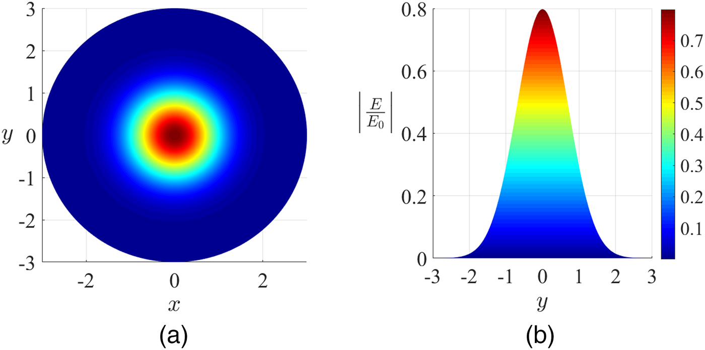
Fig. 1. Normalized electric field distribution of a Gaussian beam in the fundamental mode ( $\varpi _0 = 1{\kern 1pt} \,{\rm m}$): (a) front view and (b) transverse view.
Although most of the radiation propagates in the fundamental mode, there is also some power in higher order modes. The percentage of each depends mostly on the type of antenna used. In some cases, the fundamental mode alone is not a good enough approximation. A more general definition allows us to define the electric field for higher order modes [Reference Goldsmith2].
Gaussian beams are therefore described by three important parameters,  $\varpi, R$, and ϕ 0:
• The beam radius,  $\varpi (z)$, is the distance to the axis at which the field drops to 1/e of its on-axis value and is generally a function of the position along the propagation direction. Its minimum value, which is characteristic of the beam, is called the beam waist radius ( $\varpi _0 $) and it is located at the beam waist point, z 0, which is defined according to a reference point (e.g. the aperture of a horn antenna). In (2) it is assumed that z 0 = 0. It can be shown that [Reference Goldsmith2] (Fig. 2),
 $$\varpi = \varpi _0 \sqrt {1 + \left( {\displaystyle{z \over {z_c}}} \right)^2}, $$
where  $z_c = (\pi \varpi _0^2 )/\lambda $ is the confocal distance, an important quantity which will be defined below.
• The radius of curvature, R(z), is the radius of curvature of a wave front at z, if the wave was plane at z = 0 (Fig. 3),
(3) $$R = z + \displaystyle{{z_c^2} \over z}.$$

Naturally, at the beam waist z = z 0 = 0 and R → ∞, typical of a plane surface.
• The beam phase shift, ϕ 0, (sometimes called the Guoy phase shift) is the difference between the on-axis wave front phase and that of a corresponding plane wave. It generally changes along z, being (Fig. 4)
(4)$$\phi _0 = \arctan \left( {\displaystyle{z \over {z_c}}} \right).$$• When studying beam transformations, it is particularly convenient to define the so-called Gaussian beam parameter, q,
(5)$$\displaystyle{1 \over q} = \displaystyle{1 \over R} - i\displaystyle{\lambda \over {\pi \varpi ^2}} $$


or (as a function of  $\varpi _0 $)
 $$q = z + iz_c. $$
• The crucial quantity after which all the other parameters are written is the confocal distance (or Rayleigh range),
(7)$$z_c = \displaystyle{{\pi \varpi _0^2} \over \lambda}. $$

This parameter sets the scale at which a Gaussian beam remains collimated (i.e. the beam's rays remain parallel, with minimum divergence). Therefore, z c parameterizes the transition between the near-field region, z ≪ z c, and the far-field region, z ≫ z c.
It is important to differentiate between the definition of the field regions of Gaussian beams from that of antennas’. The antenna's near-field is the region where non-radiative fields dominate, while the far-field is associated with the emission of radiation. On the other hand, since Gaussian beams are a representation of electromagnetic waves, the field regions are always related to the beam of radiation and the way it behaves and propagates. The diffraction is the major differentiator between the near- and far-field of Gaussian beams, with z c being the transition region.
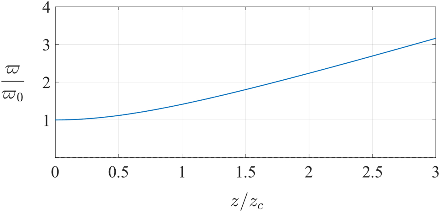
Fig. 2. The normalized beam radius is plotted as a function of the propagation axis, z.
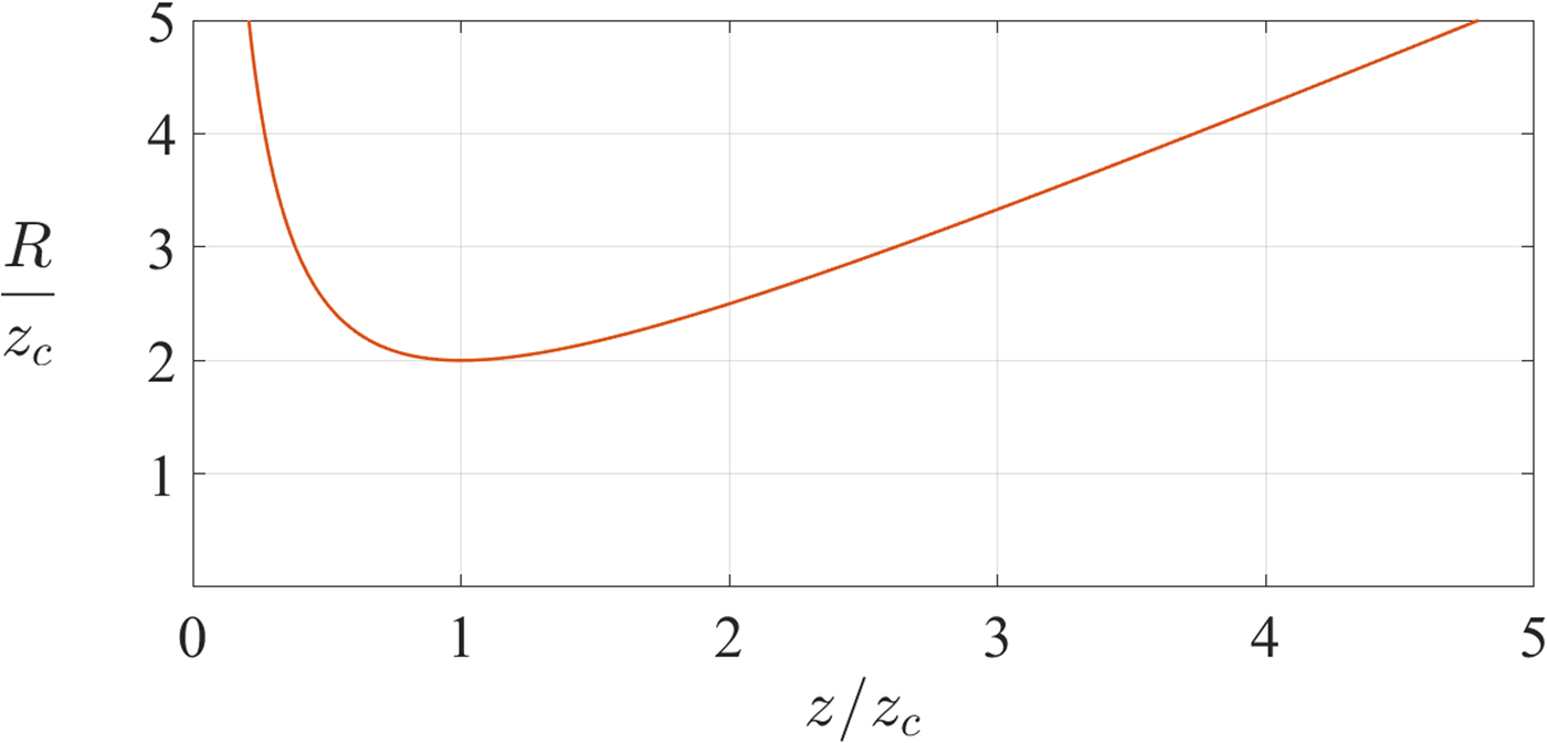
Fig. 3. The radius of curvature of the wave front along z.
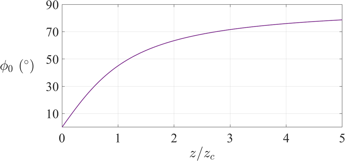
Fig. 4. Phase shift along z.
B) Paraxial approximation
The paraxial approximation refers to near axis wave fronts. These have wave vectors (rays) that are almost parallel to the optical axis at any point (i.e. the divergence angle is  $\theta\, {\rm \lesssim}\, 10^ \circ $). In such an approximation,
 $$\sin \theta \approx \theta, \quad \tan \theta \approx \theta, \quad {\rm and}\quad \cos \theta \approx 1.$$
and the analysis is linear. Generally, the paraxial approximation is considered valid as long as
 $$\displaystyle{{\varpi _0} \over \lambda} \,{\rm \gtrsim}\, 0.9.$$
However, studies of Gaussian beams beyond the paraxial limits can be found in [Reference Karandikar35, Reference Friberg, Jaakkola and Tuovinen36].
C) Beam transformation
Rays propagating freely in a homogeneous medium can be ascribed at each point to their distance (R) and slope (θ) to the optical axis. If a ray encounters a quasi-optical component, it is formally transformed and an output ray will emerge. In the paraxial approximation, these transformations are linear; hence, the output ray is linearly related to the input one:
 $$\left[ {\matrix{ {r_{out}} \cr {\theta _{out}} \cr}} \right] = \left[ {\matrix{ A & B \cr C & D \cr}} \right] \cdot \left[ {\matrix{ {r_{in}} \cr {\theta _{in}} \cr}} \right].$$
The ABCD elements form the so-called ray transfer matrix (M), which is characteristic of the system with its components. It can be calculated by multiplying the matrices of each component that interacts with a ray in reverse order (e.g. if a ray enters a system and encounters the component A and then B, the overall matrix is M = M B × M A).
The radius of curvature of the wave front of a beam is R = r/θ, and therefore, the Gaussian beam parameter, q, can be related to the ray parameters. Defining q in as the input Gaussian beam parameter at the input beam waist, we can arrive at the output Gaussian beam parameter (at the output beam waist), q out,
 $$q_{out} = \displaystyle{{A \cdot q_{in} + B} \over {C \cdot q_{in} + D}}.$$
 By using (5), we can obtain the beam radius ( $\varpi $) and the radius of curvature (R) of the output beam as a function of z.
A general system matrix, M sys, can be written by taking the matrices representing the propagation of the incoming and outgoing rays together with the ray transfer matrix, M. It enables us to write the input and output parameters for any system configuration in simple terms:
 $$\eqalign{M_{sys}& = \left[ {\matrix{ 1 & {d_{out}} \cr 0 & 1 \cr } } \right] \cdot \left[ {\matrix{ A & B \cr C & D \cr } } \right] \cdot \left[ {\matrix{ 1 & {d_{in}} \cr 0 & 1 \cr } } \right]\cr & = \left[ {\matrix{ {A + Cd_{out}} & {Ad_{in} + B + d_{out}(Cd_{in} + D)} \cr C & {Cd_{in} + D} \cr } } \right]\cr & = \left[ {\matrix{ {{A}^{\prime}} & {{B}^{\prime}} \cr {{C}^{\prime}} & {{D}^{\prime}} \cr } } \right],} $$
where d in, the input distance, is the distance from the input beam waist to the first element of the system and d out is the output distance from the last element of the system to the output beam waist (see Fig. 5).
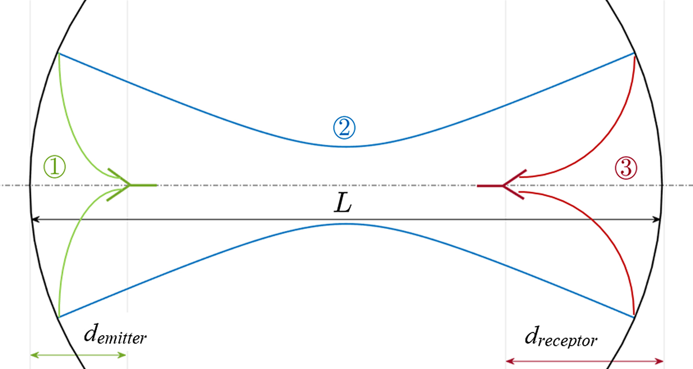
Fig. 5. Double-reflector configuration. d emitter is the distance from the input beam waist radiated by the emitter antenna to the first reflector, after which one can find a beam waist clearly located at z = L/2. d receptor is the distance from the final reflector to the output beam waist, at the reception antenna.
Since the beam parameter (6) at the beam waist (where z = 0) is q in = iz c then, by inserting A′B′C′D′ elements of the overall matrix, M sys, in (9), the output beam parameter q out becomes,
 $$q_{out} = \displaystyle{{(A + Cd_{out} )iz_c + [(A + Cd_{out} )d_{in} + (B + Dd_{out} )]} \over {Ciz_c + Cd_{in} + D}},$$
and, given that at the output beam waist, z out = 0, q out is imaginary,
 $$d_{out} = - \displaystyle{{(Ad_{in} + B)(Cd_{in} + D) + ACz_c^2} \over {(Cd_{in} + D)^2 + C^2 z_c^2}} $$
and finally the output beam waist radius  $\varpi _{0_{out}} $ (knowing that $\det M = 1$),
 $$\varpi _{0_{out}} = \displaystyle{{\varpi _{0_{in}}} \over {\sqrt {(Cd_{in} + D)^2 + C^2 z_c^2}}}. $$
D) Gaussian coupling efficiency, the beam waist radius ($\varpi _0 $) and its location (z 0)

The Gaussian coupling efficiency (η G) translates the amount of power from an antenna which is coupled to the fundamental Gaussian beam (with a certain  $\varpi _0 $ and z 0) [Reference Sheppard and Saghafi37]. When designing an antenna as a function of $\varpi _0 $, it is important to maximize η G.
In [Reference Goldsmith2], some antenna types have their η G discriminated as well as the correspondent  $\varpi _0 $ and z 0. However, for different types of antenna, one can still arrive at the Gaussian coupling efficiency by an algorithm explained in [Reference Sheppard and Saghafi37]. This is especially relevant when considering the sub-efficiencies which amount to η G.
The quantities explained in this section are fundamental when designing a concrete system because only with them can the antennas be approximated to Gaussian beams.
II. QUASI-OPTICAL SYSTEM
The proposed quasi-optical system for this study is a double-reflector configuration (represented in Fig. 5), somewhat inspired by the acoustic mirror. The idea is that:
1. A feed antenna radiates on the first reflector;
2. The mirror transforms the radiation in order for it to better propagate through space, directing the beam at the second mirror;
3. This last one will in turn transform the beam, so that it can be better received in the final antenna.
Although represented on-axis, an offset reflector should be mandatory since most energy flows in the center of the axis. This set-up was chosen for being the most simple (reflectors are the only type of components used besides the mandatory feed antennas) which serves the purpose of theory validation and preparation for more advanced systems (e.g. adding lenses will enable increasingly complex and improved solutions). Parabolic reflectors were chosen in order to avoid spherical aberration.
The separation between reflectors (L) is the quantity that specially characterizes the system. Our final goal is to understand how to achieve the maximum power transmission efficiency, for the maximum L possible.
It is extremely necessary to make a note here. Every quasi-optical system analysis is made by considering an incident beam, with a certain beam waist radius  $\varpi _{0_{in}} $ located at a distance d in from the first component of the system, that suffers transformations by the system. The result is an output beam with a certain $\varpi _{0_{out}} $ that will be located at a distance d out from the last component of the system. A representation of a general quasi-optical system is represented in Fig. 6.
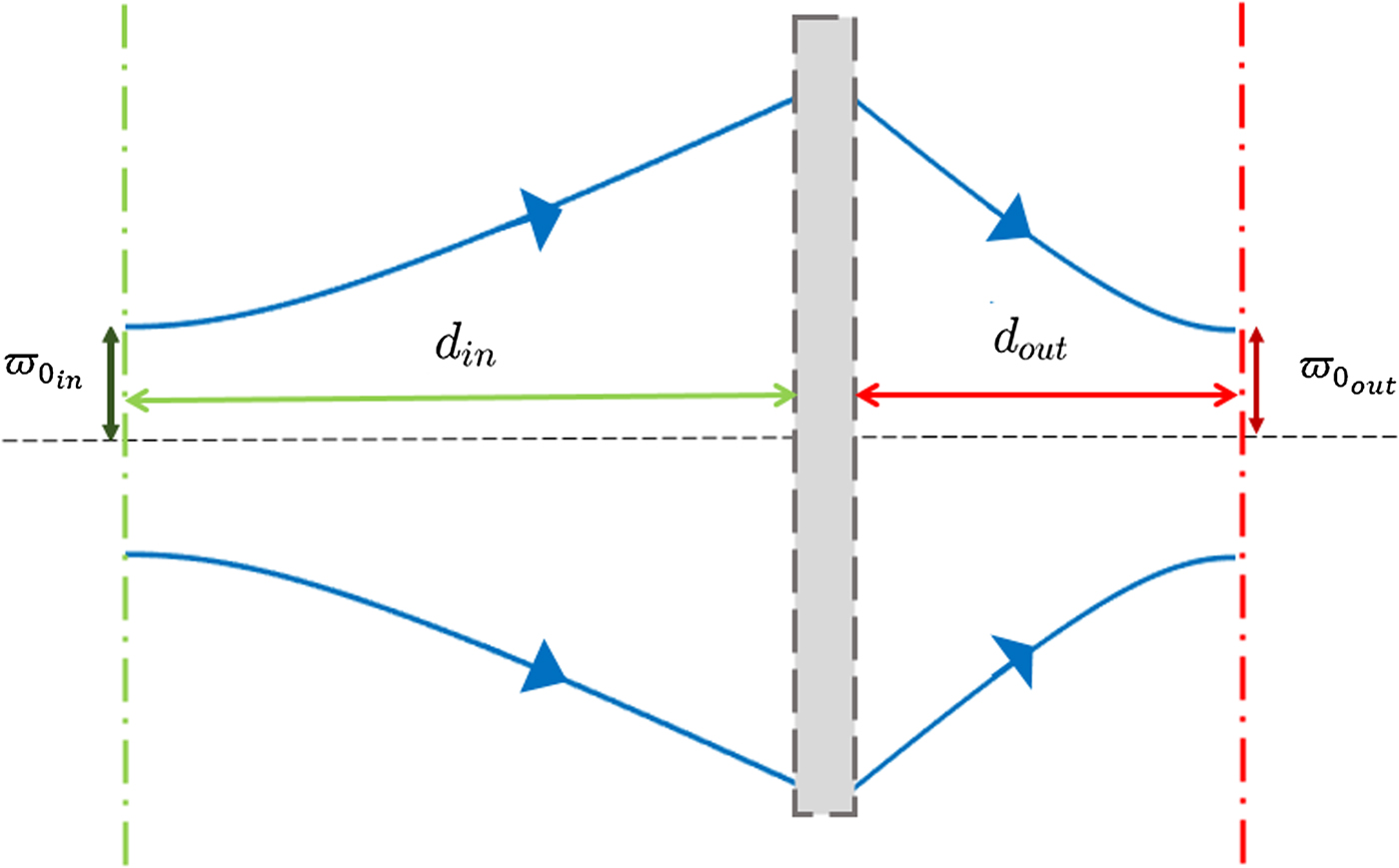
Fig. 6. General quasi-optical system. d in is the distance from the input beam waist to the first system's component, whereas d out is the distance from the final component to the output beam waist. The gray box illustrates the general system which can be composed of various components.
For our double-reflector system, the quasi-optical system is composed of three components: the first reflector, the distance between reflectors and the final reflector, where d′in = d emitter, d′out = d receptor (the inverted comas are used for quantities referring to the total double-reflector system).
However, we can begin our analysis by simplifying the double mirror set-up by making both mirrors and antennas equal: in optics and quasi-optics, rays respect the reciprocity principle; therefore, the same laws apply to incoming or outgoing beams – the transformations are simply reversed. One can then analyze the mirrors’ effect by studying only one of them. It is important to note that this is not a necessary step, it only simplifies the analysis (the final results will be quadratic equations instead of cubic).
By doing so, the quasi-optical system represents only one reflector and although d in = d emitter remains exactly the same, the output beam waist will now be the beam after the first reflector. By observing Fig. 5, it is clear that d out = L/2.
To summarize, the input beam waist is located at a distance d in = d emitter from the first reflector, where the emitting antenna will be. After the first reflection, the output beam will converge until it reaches its minimum value of beam radius at a certain point d out. The beam will then diverge until it arrives at the second reflector. In order to respect the reciprocity principle, it is necessary to guarantee that d out is located at exactly half the distance between the mirrors, d out = L/2: only then will the beam diverge to the second reflector in the same way as it converged from the first one, enabling the transformation by the second reflector to be reciprocal of that done by the first one. In that case, d emitter = d receptor.
In that case, the ray transfer matrix is exactly that of a single mirror with a certain focal length (f),
 $$\left[ {\matrix{ 1 & 0 \cr { - {\textstyle{1 \over f}}} & 1 \cr}} \right].$$
To clarify, the feed antenna originates a beam whose beam waist is at a certain distance d in from the reflector. This beam will diverge until it is transformed by the reflector. The output beam will converge until it reaches L/2 where the output beam waist is located by definition (i.e. d out = L/2). That finalizes the quasi-optical system analysis, but not the beam propagation, which proceeds until the receptor. Because of reciprocity, the beam is expected to diverge until it reaches L, the position where the second mirror is, with the same characteristics (parameters’ values) it had in the first mirror. Then the beam will be transformed by the mirror and focused at the receiving antenna, which, reciprocally, is at a distance of d in from the last reflector. In this case d emitter = d receptor = d in.
In the end, the incoming beam at the receiving antenna should have the same characteristics of the outgoing beam at the transmitting antenna,
 $$\varpi _{0_{final}} = \varpi _{0_{initial}}. $$
At this point, the wave front is approximately a plane wave, which might be advantageous for conversion efficiency (at the receptor).
By substituting the parameters of (14): A = 1, B = 0, C = −1/f, and D = 1 into (11) and (12), and solving as a function of the mirror's focal length (f) we arrive at
 $$af^2 + bf + c = 0,$$
with $a = \displaystyle{L \over 2} + d_{in}, \;b = - \left( {Ld_{in} + d_{in}^2 + z_c^2} \right),\;{\rm and}\;c = \displaystyle{L \over 2}\left( {d_{in}^2 + z_c^2} \right).$$
This is a quadratic polynomial equation, which has two solutions. In order for the focal length to be a real quantity
 $$b^2 - 4ac \ge 0.$$
Therefore,
 $$\left[ { - \left( {Ld_{in} + d_{in}^2 + z_c^2} \right)} \right]^2 \,-\; 4\left[ {\displaystyle{L \over 2} + d_{in}} \right]\left[ {\displaystyle{L \over 2}\left( {d_{in}^2 + z_c^2} \right)} \right] \ge 0,$$
which can be solved for L, yielding the condition,
 $$L \le z_c + \displaystyle{{d_{in}^2} \over {z_c}}. $$
III. RESULTS
A) Maximum distance between mirrors
We have arrived at an interval of possible values for L, ranging from zero up to  $L_{max} (d_{in}, z_c ) = z_c + d_{in}^2 /z_c $.
For the sake of simplicity, L will always refer to its maximum value.
In order to maximize the distance between mirrors, it is necessary to optimize on z c and d in. Hence,
 $$\left\{ {\matrix{ {\displaystyle{{\partial L} \over {\partial z_c}} = 1 - \displaystyle{{d_{in}^2} \over {z_c^2}} = 0 \Rightarrow z_c^2 = d_{in}^2 \Rightarrow z_c = \pm d_{in}} \hfill \cr {\displaystyle{{\partial L} \over {\partial d_{in}}} = \displaystyle{{2d_{in}} \over {z_c}} = 0 \Rightarrow d_{in} = 0} \hfill \cr}} \right..$$
The only critical point is therefore z c = d in = 0, which is obviously of no interest since we look forward to quantities that have positive non-zero values. Hence, it should be assumed that d in is a controllable parameter and optimize for z c.
In doing so we find that L is minimum at z c = d in, given that
 $$\displaystyle{{d^2 L} \over {dz_c ^2}} = \displaystyle{{2d_{in}^2} \over {z_c^3}} = \displaystyle{2 \over {z_{c_{crit}}}} \gt 0.$$
The function L(z c) is represented in Fig. 7 for different values of d in.
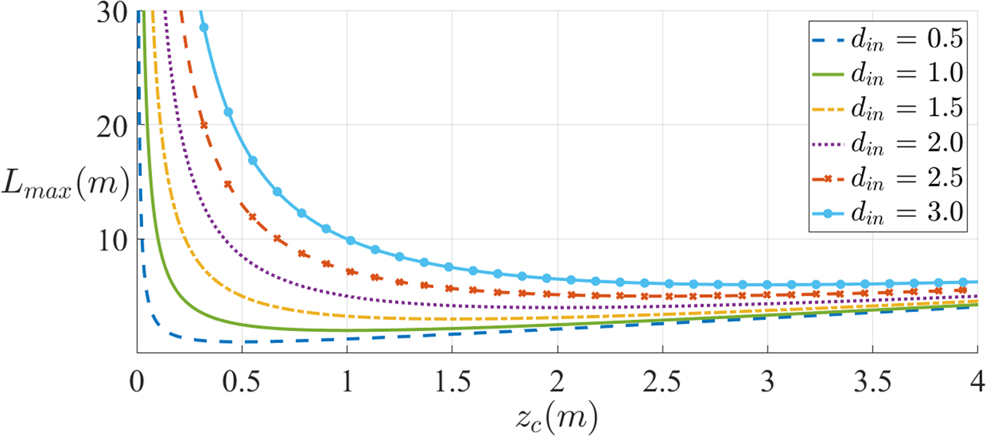
Fig. 7. Distance between mirrors, L, for different values of d in.
It is convenient to consider separately the regions below and above the minimum of L, L min = 2d in. For each of the regions, an assumption can be made, which allows for a simplification of L. These regions correspond, respectively, to
 $$z_c\, {\rm \ll}\, d_{in} \Rightarrow L \approx d_{in}^2 /z_c$$
and
 $$z_c\, {\rm \gg}\, d_{in} \Rightarrow L \approx z_c,$$
which means that in the two regions the beam is propagating in the far- and near-field, respectively. To avoid any possible ambiguity with near- and far-field antennas, we shall call the above regions simply regions 1 and 2 or instead small and big beam regions because, as will be seen in Section IV, for a certain frequency of operation, the size of the beam waist radius is much smaller in region 1 than it is in region 2.
Two conclusions are immediately obvious. For a smaller d in, L reaches the two approximations more rapidly. On the other hand, however, for a fixed z c, a smaller d in enables a smaller distance L.
The equation  $L = z_c + d_{in}^2 /z_c $ can also be written as
 $$z_c^2 - Lz_c + d_{in}^2 = 0,$$
and hence
 $$z_c = \displaystyle{{L \pm \sqrt {L^2 - 4d_{in}^2}} \over 2}$$
(meaning that  $L\,{\rm \gtrsim}\, 2d_{in} $ as above). These solutions correspond to the above regions 1 and 2, respectively.
The input distance of d in = 1 m has been chosen for convenience while remaining a reasonable distance to implement the feed circuit. All the remaining analyses will be based on this value. The function will therefore assume the curve in Fig. 8.
Fig. 8. Distance between mirrors for d in = 1 m, where the approximations for each region are visible. In the regions well below and well above the minimum, for  $z_c\; {\rm \lesssim}\; 0.1\,{\rm m}$ and $z_c \;{\rm \gtrsim}\; 5\,{\rm m}$, L can be approximated by $d_{in}^2 /z_c $ and z c, respectively.
B) Focal length
We can also obtain the focal length of the reflectors from (15). Since f has a double solution when  $L = z_c + d_{in}^2 /z_c $, then
 $$f(z_c, \;d_{in}, \;L) = \displaystyle{{Ld_{in} + d_{in}^2 + z_c^2} \over {L + 2d_{in}}}. $$
C) Beam in the far-field (region 1, where $L \approx d_{in}^2 /z_c $)

Assumption (18a) means that the beam propagates in the far-field region (region 1). The beam waist radius is, from (7),
 $$\varpi _{0_S} = \sqrt {\displaystyle{{\lambda d_{in}^2} \over {\pi L}}}, $$
where “s” stands for “small waist”. In such a case,
 $$\displaystyle{{\varpi _{0_S}} \over {\sqrt \lambda}} = \displaystyle{{d_{in}} \over {\sqrt {\pi L}}} = const,$$
which means that the ratio between the beam waist and the square root of the wavelength is a constant of the system. Therefore, if ν is the frequency and n is the refraction index of the propagation medium (n ≈ 1 for air), then
 $$\nu = \displaystyle{{cd_{in}^2} \over {\pi nL\varpi _{0_S} ^2}}. $$
This means that the choice of the components’ size will be balanced with the frequency of operation.
In region 1, the focal length is
 $$f_S = \displaystyle{{L^3 d_{in} + L^2 d_{in}^2 + d_{in}^4} \over {L^3 + 2L^2 d_{in}}}. $$
D) Beam in the near-field (region 2, where L ≈ z c)
It is apparent from Fig. 8 that the near-field is a good approximation for  $z_c \,{\rm \gtrsim}\, 5\,{\rm m}$.
In this case, the beam waist radius from (7) is
 $$\varpi _{0_B} = \sqrt {\displaystyle{{\lambda L} \over \pi}}, $$
where the subscript “B” means “big waist”. This also means that,
 $$\displaystyle{{\varpi _{0_B}} \over {\sqrt \lambda}} = \sqrt {\displaystyle{L \over \pi}} = const,\quad \quad \nu = \displaystyle{{Lc} \over {\pi n\varpi _{0_B} ^2}}. $$
Moreover, the focal length is
 $$f_B = \displaystyle{{L^2 + Ld_{in} + d_{in}^2} \over {L + 2d_{in}}}. $$
E) Paraxial limit
The paraxial approximation sets a limit for both of these regions. From (8),
 $$\displaystyle{{z_c} \over {\varpi _0}} \gt 0.9\pi, $$
and hence considering the conditions in (18), the paraxial limits for the regions 1 and 2 are, respectively,
 $$\displaystyle{{\varpi _{0_S} L} \over {d_{in}^2}} \lt \displaystyle{1 \over {0.9\pi}}$$
and
 $$\displaystyle{{\varpi _{0_B}} \over L} \lt \displaystyle{1 \over {0.9\pi}}.$$
These limits should be respected when designing the system in the paraxial approximation.
F) Beam radius at the reflector
The beam radius at the position of the reflector,  $\varpi _R $, having traveled d in, is
 $$\varpi _R = \varpi _0 \sqrt {1 + \left( {\displaystyle{{d_{in}} \over {z_c}}} \right)^2}. $$
This means that for the regions considered, we arrive at the same value,
 $$\varpi _{R_S} = \varpi _{R_B} = \sqrt {\displaystyle{\lambda \over \pi} \displaystyle{{(L^2 + d_{in}^2 )} \over L}}. $$
G) Relation between focal lengths
The quotient between (25) and (27) gives
 $$\displaystyle{{f_S} \over {f_B}} = \displaystyle{{L^3 d_{in} + L^2 d_{in}^2 + d_{in}^4} \over {L^4 + L^3 d_{in} + L^2 d_{in}^2}}, $$
which is <1 for d in < L, which will always be the case. We then have
 $$f_S \lt f_B. $$
H) Comparison between beams in the near- and far-field
In order to best understand the differences between both beam types, Fig. 9 shows the two different possible scenarios.
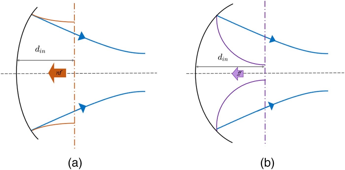
Fig. 9. Comparison between beams in the near- and far-field: (a) beam in the far-field (small) (b) beam in the near-field (big).
It is worth pointing out that the focal length representation is according to the result in the previous section.
I) Parabolic reflector
The dimensions of a parabolic reflector are related as
 $$4fD = R_R^2, $$
where R R is the reflector's radius, D its depth, and f is the focal length.
The size of R R must necessarily take  $\varpi _R $ into account, for obvious reasons. By defining the reflector's coefficient (c R) as
 $$R_R = c_R \varpi _R \quad \Rightarrow \quad \displaystyle{{R_R} \over {\sqrt \lambda}} = c_R \sqrt {\displaystyle{{(L^2 + d_{in}^2 )} \over {\pi L}}} $$
and by substituting (31) one arrives at
 $$D = \displaystyle{{c_R^2 \varpi _R^2} \over {4f}}\quad \Rightarrow \quad \displaystyle{D \over \lambda} = \displaystyle{{\;c_R^2} \over {4\pi f}}\left( {\displaystyle{{L^2 + d_{in}^2} \over L}} \right).$$
 The coefficient c R should be as large as possible, though a value of  $\sqrt 2 $ is enough from a practical point of view (Fig. 1).
It is worth noting that due to (33), D S >D B. A beam in the far-field demands a larger reflector depth.
J) Elliptic reflector
While at first elliptic reflectors they may not seem very useful for our study that is not the case.
Ellipses are defined by two foci, F 1 and F 2, and if the beam originates at the first focus, the reflecting surface (centered at a point P) will direct the output beam waist to the second focus of the ellipse, as can be seen in Fig. 10, disabling the possibility of a reciprocal system.
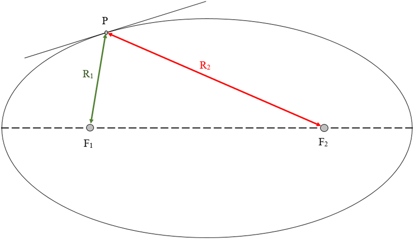
Fig. 10. General ellipse representation with its main parameters. P is any point in the surface distanced away from the foci, F 1 and F 2, by  $R_1 = \overline {F_1 P} $ and $R_2 = \overline {F_2 P} $.
The focal length of the elliptic reflecting surface centered in P is given by
 $$f_e = \displaystyle{{R_1 R_2} \over {R_1 + R_2}}, $$
where  $R_1 = \overline {F_1 P} $ and $R_1 = \overline {F_2 P} $.
To obtain the optimal performance of an elliptical focusing surface [Reference Goldsmith2], we need to set the system in a way that the input beam has a value of radius of curvature such that R in = R 1 and, similarly, the radius of curvature of the output beam R out = R 2.
Although the use of elliptical reflectors made from surfaces of the same ellipse is not advantageous, we can use the surface from two equal ellipses which share one focal point (Fig. 11), thus arriving at a situation where the reciprocal principle is again obtainable.
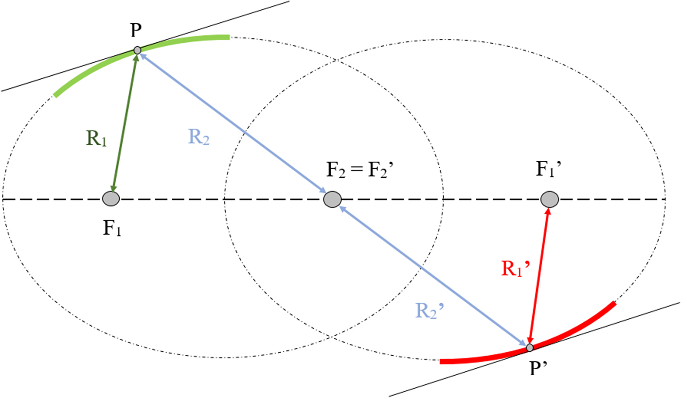
Fig. 11. Double ellipse system. The second ellipse parameters are denoted by an inverted comma. The ellipses share one focus point, F 2 = F′2, and, to respect reciprocity, R 1 = R′1 and R 2 = R′2.
Gaussian beams in that system are represented in Fig. 12. It is worth noting that, to satisfy the optimal condition for elliptical reflector, the requirement is not for the input beam waist to be located in the focus point, F 1, but for the input beam to have a value of radius of curvature at the reflector of R in = R 1.
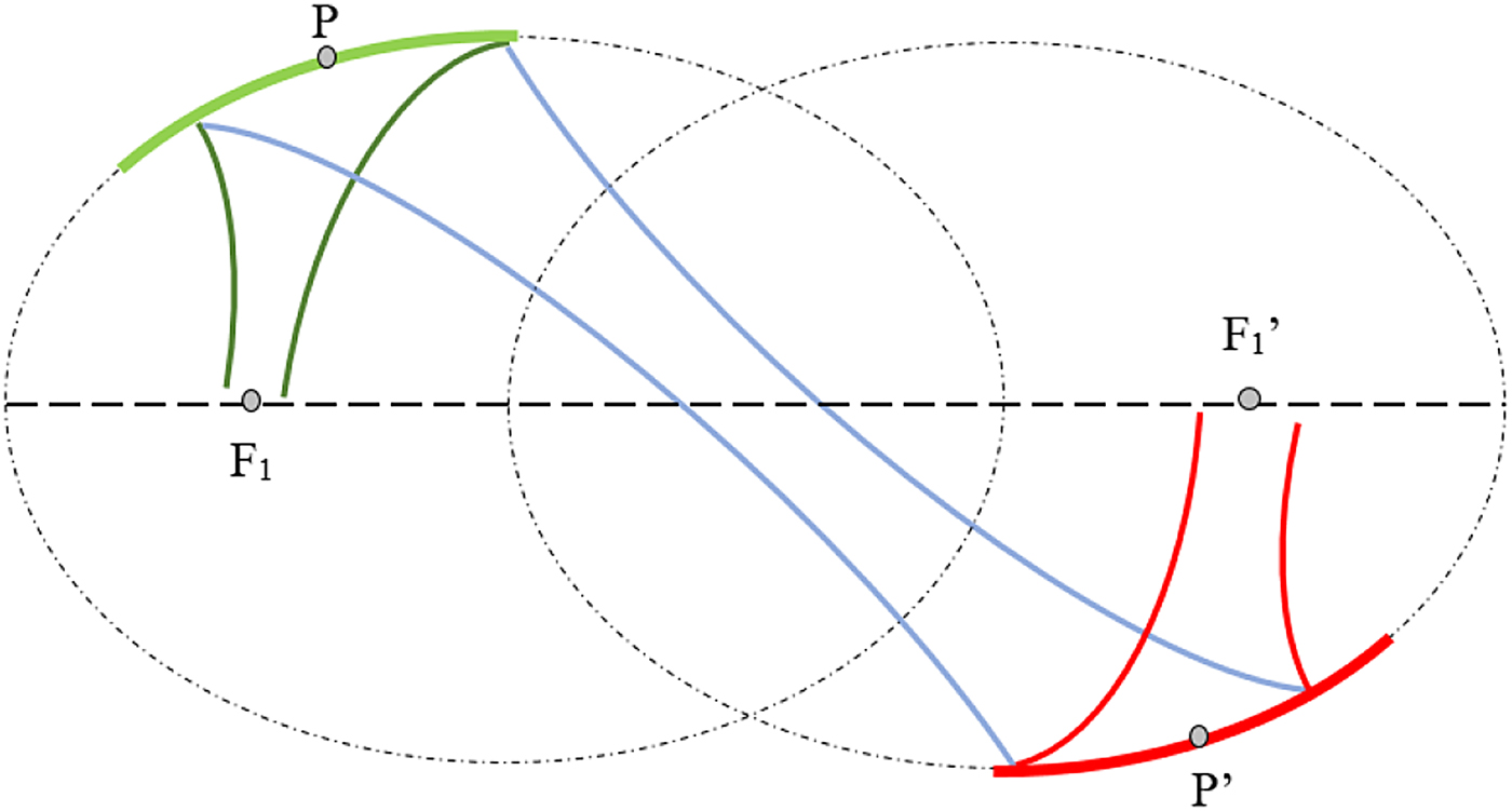
Fig. 12. Schematic representation of a double ellipsoidal reflector quasi-optical system. The distance between mirrors is simply  $L = \overline {PP'} $. To obtain the optimal condition, the input and ouptut beam waist must be located at a point which makes $R_{in} = R_1 = \overline {F_1 P} $ and $R_{out} = R'_1 = \overline {F'_1 P'} $.
K) Ellipsoidal focal length validity
We will verify if the focal length of an ellipsoidal surface is equivalent to that of a general quasi-optical component.
As stated before, the focal length of an ellipsoidal reflector in the optimal quasi-optical condition is given by f e = (R in R out)/(R in + R out). From (3), we have that
 $$\eqalign{R_{in} & = d_{in} + \displaystyle{{(\pi \varpi _{0_{in}} ^2 /\lambda )^2} \over {d_{in}}} \quad \quad {\rm and} \cr & \quad R_{out} = d_{out} + \displaystyle{{(\pi \varpi _{0_{out}} ^2 /\lambda )^2} \over {d_{out}}}.}$$
Now, since the ray transfer matrix of a reflector is generally given by A = 1, B = 0, C = −1/f, and D = 1, by replacing its values in (12) and (13), we get
 $$\varpi _{0_{out}} = \displaystyle{{(z_c^2 + d_{in}^2 /f) - d_{in}} \over x}$$
and
 $$\varpi _{0_{out}} = \displaystyle{{\varpi _{0_{in}}} \over {\sqrt x}}, $$
where  $x = (f^2 - 2fd_{in} + d_{in}^2 + z_c^2 )/f^2 $. The elliptical focal length becomes
 $$\eqalign{\displaystyle{{\left( {d_{in} + \displaystyle{{z_c^2} \over {d_{din}}}} \right)\left( {d_{out} + \displaystyle{{z_c^2} \over {d_{dout}}}} \right)} \over {d_{in} + \displaystyle{{z_c^2} \over {d_{din}}} + d_{out} + \displaystyle{{z_c^2} \over {d_{dout}}}}} = \ldots = \displaystyle{1 \over {\displaystyle{{d_{out}} \over {z_{c_{out}} ^2 + d_{out}^2}} + \displaystyle{{d_{in}} \over {z_{c_{in}} ^2 + d_{in}^2}}}}.} $$
At this point, we can use (39) and (40) to arrive at the final form,
 $$f_e = f.$$
We have proven that the focal length is indeed valid.
L) Theory restraints
For the value of the distance between reflectors, L, we have two different equationsFootnote 1. One arises immediately from the quasi-optical formalism as L 1 = 2d out, where d out is given by (12). The other (L 2) is calculated from (21). The starting point is that these should be the same:
 $$L_1 = 2f\displaystyle{{z_c^2 + d_{in}^2 - fd_{in}} \over {f^2 - 2fd_{in} + z_c^2 + d_{in}^2}} = \displaystyle{{z_c^2 + d_{in}^2 - 2fd_{in}} \over {f - d_{in}}} = L_2. $$
After working on the terms as a function of f, we arrive at
 $$f^2 (d_{in}^2 - z_c^2 ) - 2fd_{in} (z_c^2 + d_{in}^2 ) + (z_c^2 + d_{in}^2 )^2 = 0,$$
which has the solution,
 $$f = \displaystyle{{z_c^2 + d_{in}^2} \over {d_{in} \mp z_c}}. $$
 By replacing (45) in L 1 and L 2, we arrive at exactly the same solution,  $L_1 = L_2 = \mp \left( {z_c + \displaystyle{{d_{in}^2} \over {z_c}}} \right)$. Since L >0, the solution of interest is
 $$f = \displaystyle{{z_c^2 + d_{in}^2} \over {z_c + d_{in}}}. $$
M) d in that maximizes L 1
In the case that  $f \ne (z_c^2 + d_{in}^2 )(z_c + d_{in} )$, we must use L 1 = 2d out = L as the distance between reflectors:
 $$L = 2f\displaystyle{{z_c^2 + d_{in}^2 - fd_{in}} \over {f^2 - 2fd_{in} + z_c^2 + d_{in}^2}}. $$
The distance d in which maximizes L is obtained by optimizing (47) as a function of d in,
 $$\eqalign{\displaystyle{{\partial L} \over {\partial d_{in}}} = \displaystyle{{ - 2f^2 (f^2 - 2fd_{in} - z_c^2 + d_{in}^2 )} \over {(f^2 - 2fd_{in} + z_c^2 + d_{in}^2 )^2}} = 0\quad \Rightarrow \quad d_{in} = f \pm z_c.} $$
 Knowing that  $\displaystyle{{\partial ^2 L} \over {\partial {\kern 1pt} d_{in} ^2}} = \mp \displaystyle{{f^2} \over {z_c^3}} $, L is maximum when,
 $$d_{in} = f + z_c. $$
N) Summary
Quasi-optical systems made up of two equal components, positioned in such a way that the reciprocity principle is respected, can be explained by two simple equations, (17) and (46), reproduced here:
 $$f = \displaystyle{{z_c^2 + d_{in}^2} \over {z_c + d_{in}}} \quad \quad {\rm and}\quad \quad L = z_c + \displaystyle{{d_{in}^2} \over {z_c}}. $$
The suggested system building procedure is as follows.
In most applications, L is normally the first variable to be defined. When that is the case, f and  $\varpi _0 $ must be adjusted to best fit the parameter requirements. $\varpi _0 $ depends heavily on the feed antenna characteristics, normally being the second parameter to be settled. Then, it is only a matter of calculating f and d in [from (17), $d_{in} = \sqrt {z_c (L - z_c )} $] to obtain all of the parameter values.
IV. CASE DISCUSSION
A script has been developed in order to verify the expected beam radius value as the beam propagates, undergoes a transformation by the reflectors and reaches the final antenna. It enables the graphical representation of the beam propagating through the system, by implementing the equations described in the paper.
A Gaussian beam is started at z 0 with a user-defined beam waist radius ( $\varpi _0 $) and direction of propagation. The position of the different components as well as their ABCD parameters must also be defined, prior to the beam propagation throughout the system, so that if the beam position coincides with that of a certain component, it will suffer a transformation, as described in the Introduction section.
Taking an input distance of d in = 1 m and a distance between reflectors of  $L = 100\,{\kern 1pt} {\rm m}$, the paraxial limit dictates that
which respectively translates into the wavelength limits,
Or
In order to arrive at an optimum system, it is necessary to consider the size of the components and the frequency of operation. Defining one quantity may lead to undesired values for the other.
The focal length of the reflectors is given by (25) and (27) for the regions concerned, yielding
 $$f_S = 0.990\,{\rm m}\quad {\rm and}\quad f_B = 99.029{\kern 1pt} {\rm m}.$$
A) Beam in the far-field (region 1)
The minimum frequency of operation for working with a small beam, for an input distance of 1 m and a distance between mirrors of 100 m, is 76.341 GHz. For easing the calculations, we choose ν = 80 GHz, and hence
 $$\lambda = 3.750 \times 10^{ - 3} {\rm m},\quad \varpi _{0_S} = \sqrt {\displaystyle{{\lambda d_{in}^2} \over {\pi L}}} = 3.455\,{\kern 1pt} {\rm mm}.$$
We obtain a relatively small beam waist radius, which will be advantageous in terms of the size of the components, while needing a high frequency of operation.
B) Beam in the near-field (region 2)
On the other hand, a big beam can have a much smaller frequency, starting at  $\nu = 8{\kern 1pt} {\rm MHz}$, giving
 $$\lambda = 37.500{\kern 1pt} {\rm m},\quad \varpi _{0_B} = \sqrt {\displaystyle{{\lambda L} \over \pi}} = 34.549{\kern 1pt} \,{\rm m}.$$
 A huge beam waist radius is obtained. However, by choosing  $\nu = 80{\kern 1pt} {\rm GHz}$, then
 $$\lambda = 3.750 \times 10^{ - 3}\; {\rm m},\quad \varpi _0 = 0.346\;{\rm m}.$$
It is worth noting that by properly choosing the frequency, the size of the beam waist radius will define if the beam is propagating in the near- or in the far-field.
C) Graphical representation
Several beams have been represented as a function of the frequency of operation (whose values were spread in order to account for different beam waist radii) from both region 1 (Fig. 13) and region 2 (Fig. 14). A logarithmic scale was used in the latter, due to the significant difference in the beam waist radius value between the beam in MHz and the remaining in GHz.
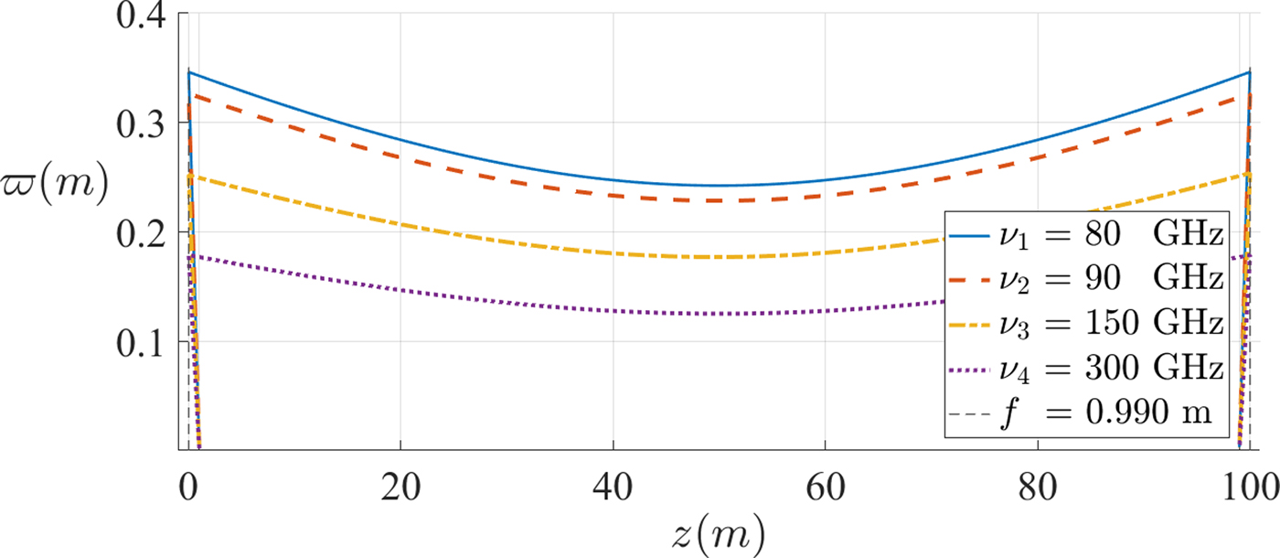
Fig. 13. Beams propagating in the far-field (region 1).  $\varpi $ is the beam radius, z is the position along the propagation direction, ν is the characteristic frequency of operation, and f is the focal distance.
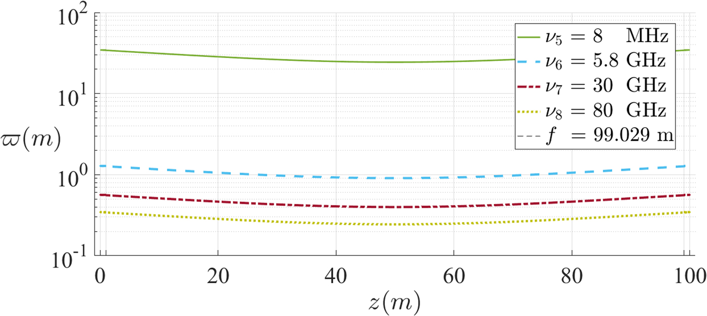
Fig. 14. Beams propagating in the near-field (region 2).  $\varpi $ is the beam radius, z is the position along the propagation direction, ν is the characteristic frequency of operation and f is the focal distance.
In order to analyze the difference between the beams propagating in each of the regimes, another plot in the near-field was made (Fig. 15), operating at the same frequencies as that in Fig. 13.
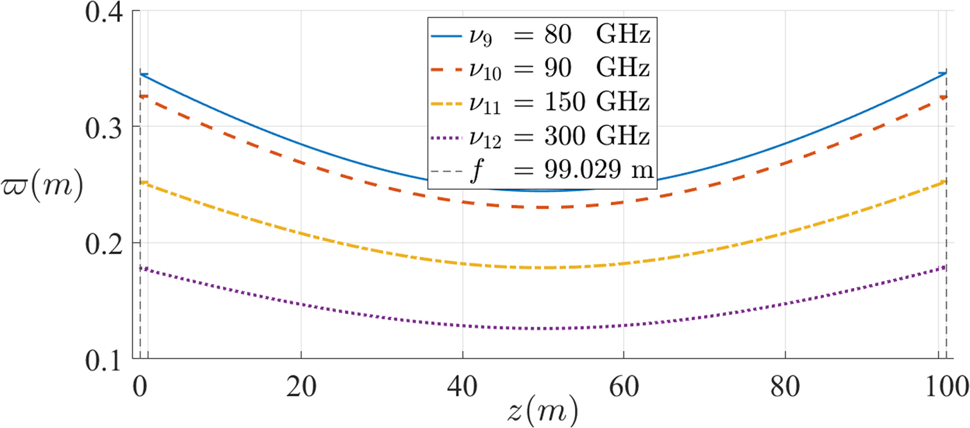
Fig. 15. Beams propagating in the near-field with the same frequency as those in Fig. 13.  $\varpi $ is the beam radius, z is the position along the propagation direction, ν is the characteristic frequency of operation, and f is the focal distance.
A few observations are in order:
• As the frequency increases, the average size of the beam radius decreases. Since the size of the antenna (reflector) is related to that of the beam waist radius (beam radius at the reflector), beams in the far-field regime appear more advantageous in this sense;
• The beam radius of the beam between the reflectors is independent of the beam type (whether it is a near- or far-field beam), which originate from the antenna. Beams in the near-field have beam radius larger than the beam radius of the beam between reflectors, while beams in the far-field have a smaller beam radius, as can be seen in Fig. 9. When implementing this study, the size of various components may be constrained, forcing us to choose a feed beam in the near- or far-field.
Regarding beams propagating with the same frequency, for either of the regimes, the beam radius at the reflector as well as the output beam waist radius (at  $L = 50{\kern 1pt} \,{\rm m}$) have nearly identical values. One can conclude that although the initial conditions have been different (emitting a beam in the near- or far-field), at the reflector and after the transformation, the beam propagating the L distance has nearly the same characteristics.
V. CONCLUSION
The theoretical study of a double-reflector quasi-optical system was presented in the paraxial approximation, discussing the beam radii of two different beam types, propagating in the near- and far-field, respectively. Different parameters have been considered for each of the beam types.
The preliminary results are consistent to what was expected considering the validity of the reciprocity between the source and the receptor. This study shows that we can have a framework simple enough in order to access the parameters concerned and to gain insight about their relevance.
We now have a tool to quickly prototype simple systems (the script enables the implementation of reflectors and lenses), which serves as a basis for more complex analyses.
Further studies are necessary to analyze the power transfer efficiency and improve the model, alongside to simulations to all the process that exhaust the parameter space and allow proper optimization. A case study of a system with a double ellipsoidal mirror is also being considered [Reference Tuan, Chou, Lu and Chou38, Reference Chou, Tuan, Lu and Chou39], although some analysis is already presented here.
Upon completion of this work, we plan on making a double-reflector prototype aimed at measuring the effect of the various parameters on the power transfer between the emitting and receptor antennas and access the validity of the paraxial calculations. Several components have already been chosen and the main system parameters shall have the following values:
The goal is to be able to transfer power over the distance of  $L = 5{\kern 1pt} \,{\rm m}$ using two conical smooth surfaced antennas, which will reflect on two parabolic reflectors with the diameter of 1 m.
We can conclude that the goal of this study was achieved since preliminary results were obtained for building a system with reduced spillover losses, important for guaranteeing that the maximum beam arrives at the receiver antenna.
 Ricardo André Mendes Pereira graduated from the University of Coimbra in 2017 with an M.Sc. degree in Physics Engineering, specializing in Instrumentation. He currently works as a Research Assistant at the same institution, studying spacecraft simulation, modeling, and control. His research interests are electromagnetism, especially wireless power transfer, space, and nuclear physics.
 Nuno Borges Carvalho (S′97–M′00–SM′05–F′15) was born in Luanda, Angola, in 1972. He received the Diploma and Doctoral degrees in Electronics and Telecommunications Engineering from the University of Aveiro, Aveiro, Portugal, in 1995 and 2000, respectively. He is currently a Full Professor and a Senior Research Scientist with the Institute of Telecommunications, University of Aveiro and an IEEE Fellow. He coauthored Intermodulation in Microwave and Wireless Circuits (Artech House, 2003), Microwave and Wireless Measurement Techniques (Cambridge University Press, 2013) and White Space Communication Technologies (Cambridge University Press, 2014). He has been a reviewer and author of over 200 papers in magazines and conferences. He is an associate editor of the IEEE Microwave Magazine and Cambridge Wireless Power Transfer Journal and former associate editor of the IEEE Transactions on Microwave Theory and Techniques. He is the co-inventor of six patents. His main research interests include software-defined radio front-ends, wireless power transmission, nonlinear distortion analysis in microwave/wireless circuits and systems, and measurement of nonlinear phenomena. He has recently been involved in the design of dedicated radios and systems for newly emerging wireless technologies. He is the Chair of the IEEE MTT-20 Technical Committee and the past-chair of the IEEE Portuguese Section and MTT-11 and also belongs to the technical committees, MTT-24, and MTT-26. He is also the Vice-chair of the URSI Commission A (Metrology Group). He was the recipient of the 1995University of Aveiro and the Portuguese Engineering Association Prize for the best 1995 student at the University of Aveiro, the 1998 Student Paper Competition (Third Place) of the IEEE Microwave Theory and Techniques Society (IEEE MTT-S) International Microwave Symposium (IMS), and the 2000 IEE Measurement Prize. He is a Distinguished Microwave Lecturer for the IEEE Microwave Theory and Techniques Society.
 José Pinto da Cunha has a Ph.D. in High Energy Physics from the University of Liverpool (UK). His research interests include data analysis, Monte Carlo simulation and event reconstruction, in particular on the optical response of radiation detectors. He has participated in various collaborations on High-energy Physics and Astrophysics and is an Assistant Professor at the Department of Physics of the University of Coimbra, Portugal.


