


Introduction
Implementing an integrated weed management (IWM) system continues to be a key aim for cotton growers in Australia and elsewhere, faced with ever-increasing pressure from weeds that have developed resistance to an expanding list of herbicides and herbicidal mechanisms of action (Charles et al. Reference Charles, Sindel, Cowie and Knox2020a, 2020b). A successful IWM system will necessarily use a combination of components, including chemical, mechanical, cultural, and genetic tools (Knezevic et al. Reference Knezevic, Evans, Blankenship, Van Acker and Lindquist2002) integrated into the farming system to manage weeds sustainably, with minimal detrimental economic and environmental damage (Korres and Norsworthy Reference Korres and Norsworthy2015; Taylor et al. Reference Taylor, Charles and Inchbold2004). An IWM system is built on an understanding of weed and crop biology, phenology, and competitiveness. Defining the critical period for weed control (CPWC) is an important step in defining weed-crop competition and is a valuable aid in developing an IWM system (Knezevic and Datta Reference Knezevic and Datta2015).
The CPWC relationship describes the period of the season during which the crop is most sensitive to weed competition, relating the estimated yield losses from competition to a chosen yield-loss threshold. The CPWC is delineated by the critical timing for weed removal (CTWR) and the critical weed-free period (CWFP). The CTWR is the period during which the crop can tolerate early-season competition before unacceptable yield loss, and the CWFP is the minimum period after crop emergence during which the crop needs to be kept free of weeds to avoid unacceptable yield losses (Knezevic et al. Reference Knezevic, Evans, Blankenship, Van Acker and Lindquist2002). The CTWR and the CWFP combine with a yield-loss threshold to define the CPWC (Charles et al. Reference Charles, Sindel, Cowie and Knox2020a; Knezevic and Datta Reference Knezevic and Datta2015; Korres and Norsworthy Reference Korres and Norsworthy2015). The yield-loss threshold depends on the value of the crop and the cost of weed control (Knezevic et al. Reference Knezevic, Evans, Blankenship, Van Acker and Lindquist2002).
The CPWC concept has been applied to many crop and weed combinations. However, the findings in cotton crops have frequently been site specific and season specific because of a diversity of factors such as weed species and density, the time of crop and weed emergence, and seasonal conditions (Bukun Reference Bukun2004; Korres and Norsworthy Reference Korres and Norsworthy2015; Tingle et al. Reference Tingle, Steele and Chandler2003; Tursan et al. Reference Tursun, Datta, Tuncel, Kantarci and Knezevic2015, 2016; Webster et al. Reference Webster, Grey, Flanders and Culpepper2009). Consequently, the findings from many studies could be applied only to the situation of the study, limiting the wider application of the findings (Charles Reference Charles, Sindel, Cowie and Knox2021, Knezevic et al. Reference Knezevic, Evans, Blankenship, Van Acker and Lindquist2002). Knezevic et al. (Reference Knezevic, Evans, Blankenship, Van Acker and Lindquist2002) proposed using growing degree days (GDD) as the measure of time in the CPWC relationships, rather than the more commonly used calendar days, in order to reduce the influence of seasonal variability on the relationships. Using GDD as the measure of time, Charles et al. (Reference Charles, Sindel, Cowie and Knox2019a, 2020a, 2020b, 2021) were able to define CPWC relationships that could be applied over multiple seasons for high-yielding cotton. However, this approach of using GDD was not always successful in other situations (Bukun Reference Bukun2004; Tursan et al. Reference Tursun, Datta, Tuncel, Kantarci and Knezevic2015, 2016; Webster et al. Reference Webster, Grey, Flanders and Culpepper2009), possibly because of the effect of variability in crop and weed populations and seasonal rainfall in these studies, variables that were not accounted for in the CPWC models.
The importance of measuring both weed and crop density and size throughout the growing season, thereby accounting for additional site and seasonal variation has been emphasized (Knezevic et al. Reference Knezevic, Evans, Blankenship, Van Acker and Lindquist2002; Zimdahl Reference Zimdahl1988), but there has been no way of incorporating this information into the CPWC relationships. Bukun (Reference Bukun2004), for example, related weed biomass and crop height to GDD throughout the season, thus explaining much of the seasonal variation in the data but was unable to use this information in developing the CPWC relationships, which consequently remained season specific.
Models that described the CPWC in cotton over a range of weed densities were developed by Charles et al. (Reference Charles, Sindel, Cowie and Knox2019a, 2020a, 2020b) by incorporating weed density as an additional term in the CTWR and CWFP models, overcoming the limitation in the CPWC relationships of variations in weed density. They further refined the models by replacing weed density with weed height and weed biomass in the relationships, culminating in a model that described the CPWC over a range of weed sizes and densities, seasons, and species (Charles et al. Reference Charles, Sindel, Cowie and Knox2021).
The models presented by Charles et al. Reference Charles, Sindel, Cowie and Knox2019a, 2020a, 2020b, 2021) were developed using three mimic weeds, common sunflower, Japanese millet [Echinochloa esculenta (A. Braun)], and mungbean [Vigna radiata (L.) R.Wilczek], that were chosen to represent a range of weed types. The use of mimic weeds in competition studies can give better experimental controllability and repeatability (Strydhorst et al. Reference Stydhorst, King, Lopetinsky and Harker2008), and the results from these studies can be related to competition from real weed species provided differences in plant dry weight and height are accounted for (Charles et al. Reference Charles, Sindel, Cowie and Knox2019b).
One of perceived strengths of the CPWC model is that it defines the period in the season by which the crop is most sensitive to weed competition, such that weeds present during the CPWC must be controlled at this time, but weeds present before or after the CPWC will not cause yield losses exceeding the yield-loss threshold (Knezevic et al. Reference Knezevic, Evans, Blankenship, Van Acker and Lindquist2002; Knezevic and Datta Reference Knezevic and Datta2015; Korres and Norsworthy Reference Korres and Norsworthy2015; Price et al. Reference Price, Korres, Norsworthy and Li2018). Knezevic et al. (Reference Knezevic, Evans, Blankenship, Van Acker and Lindquist2002) reported that specialists and consultants have described the CPWC “as a window in the crop growth cycle during which weeds must be controlled”. However, this definition of the CPWC may not be strictly correct, with the CPWC better defined as “a span of time between that time period after seeding or emergence, when competition does not reduce crop yield, and the time after which weed competition will no longer reduce crop yield” (Zimdahl Reference Zimdahl1988).
The differences between these definitions lies in understanding the method used to define the CWFP curve, which delimit the end of the CPWC. The CWFP curve is generated by measuring the yield loss caused by weeds that emerge after crop emergence and go on to compete for the remainder of the cropping season. By definition, the competitive effect of a weed that emerges at the limit of the CWFP does not exceed the yield-loss threshold until the end of the cropping season. Hence, some of the competitive effect of weeds that emerge during the CPWC may be occurring after the end of the CPWC, such that weeds that emerge late in the CPWC will not need to be controlled until after the end of the CPWC in order to prevent yield losses exceeding the yield-loss threshold. Thus, the intersection of the CWFP with the yield-loss threshold delimits the point beyond which weeds that emerge will not cause economic damage to the crop if they are not controlled (Zimdahl Reference Zimdahl1988), not the point at which emerged weeds need to be controlled (15; Knezevic et al. Reference Knezevic, Evans, Blankenship, Van Acker and Lindquist2002; Knezevic and Datta Reference Knezevic and Datta2015; Korres and Norsworthy Reference Korres and Norsworthy2015; Price et al. Reference Price, Korres, Norsworthy and Li2018). Weeds that emerge after the start of the CPWC, but still within the CPWC, need to be controlled to prevent unacceptable yield losses (Zimdahl Reference Zimdahl1988), but do not necessarily need to be controlled during the CPWC. The CPWC model gives no information on the necessary timing of the control of these weeds.
In practice, some delay in the implementation of a control measure after initial weed emergence allows for additional weed emergence to occur, thereby increasing the number of weeds controlled by a single management input and improving production efficiency (Taylor et al. Reference Taylor, Charles and Inchbold2004). This delay in weed control is acceptable, provided weeds are still controlled by the management tool before the yield-loss threshold is exceeded. In many situations, the limitations of the management tools used to control weeds may determine the timing of the control input, because it is always easier to kill small plants rather than large plants, regardless of the method used (Zimdahl Reference Zimdahl1988). Nevertheless, an understanding of the optimal timing of control of these later emerging weeds is an important component of a weed management system to be used by farmers (Swanton and Weise Reference Swanton and Weise1991; Werth et al. Reference Werth, Boucher, Thornby, Walker and Charles2013).
The objective for our study was to quantify the reductions in crop yield from later weed germination events within the CPWC, over a range of seasons and weed densities. We tested the hypothesis that weeds emerging during the CPWC did not necessarily need to be controlled during the CPWC to prevent yield losses exceeding the yield-loss threshold. We describe the relationships using extended CTWR and CWFP functions and determine the point at which these weeds needed to be controlled to prevent crop damage exceeding the weed-control threshold.
Materials and Methods
Field studies were conducted over three seasons from 2005 to 2008 at the Australian Cotton Research Institute, in Narrabri NSW (30.12°S, 149.36°E; elevation 201 m) on a heavy alluvial clay (fine, thermic, smectitic, Typic Haplustert) soil. Cotton crops were grown on raised hills, 1 m apart, in line with standard commercial practices, using the cotton cultivar ‘Sicot 80 BRF’. Fields were fertilized with 180 kg N ha−1, applied before planting, and were flood-irrigated as required, in line with standard industry practices. Cotton was planted at 15 seeds m−1 on October 19, 2005; October 6, 2006; and October 8, 2007. The common sunflower cultivar ‘Hyoleic 43’ was planted in 2005, and ‘Hysun 38’ in 2006 and 2007 in rows adjacent to, and offset from, the cotton by 100 mm. Plots were otherwise maintained weed free with trifluralin (Triflur X®, 480 g L−1; Nufarm Australia, Melbourne, Victoria, Australia) at 1.1 kg ha−1, incorporated to 5 cm before planting using a disc cultivator. Weeds were managed using glyphosate (Roundup Ready® Herbicide, 690 g kg−1; Monsanto Australia, Melbourne, Victoria, Australia) broadcast after crop planting (POST) at 1 kg ai ha−1 as required over weed-free plots, and hand hoeing was performed where needed.
Experimental Design
The experiments used a randomized, complete block design with split plots and four replications; subplots were four rows (4 m) wide by 10 m in length, with a 2-m buffer between plots. Main plots were times of weed planting and removal, and subplots were weed densities. Common sunflower was planted with the crop or at predetermined periods after crop emergence, sown to achieve target densities of 2, 5, 10, and 20 plants m−2.
Times of weed planting and removal were measured in GDD since planting (Equation 1), defined as:
 $$T = \sum {\rm{ }}{{\left( {{t_{min}}\; + \;{t_{max}}} \right)} \over 2} - {t_b}$$
where t min and t max were the daily minimum and maximum air temperatures, respectively, and t b was the base temperature of 15.5 C (Bukun Reference Bukun2004).
Times of weed addition were planned to occur at 0, 150, 300, and 450 GDD. Times of weed removal were planned to occur at 0, 200, 400, 600, and 800 GDD after weed addition, and at crop maturity. Actual densities of established common sunflower, and times of planting and removal, were influenced by rainfall and irrigation events, with weed emergence delayed by inadequate soil moisture on some occasions. Not all target weed densities and timings were achieved in all seasons.
Weed density was recorded on 1 m of row in each plot at the time of weed removal. For analysis, data were grouped by density such that the average weed density of each group equated as closely as possible to the nominal densities of 2, 5, 10, and 20 common sunflower plants m−2. Cotton was mechanically harvested using a commercial cotton picker modified to pick a single row, and seed-cotton yield was recorded from each of the central two rows of each plot. A single-saw gin was used to determine ginning percentage and lint yield from subsamples from one row of each plot.
Statistical Analysis
The data sets were analyzed using R statistical software, version 3.6.3 (R Foundation for Statistical Computing, Vienna, Austria) with a significance level of P < 0.05. The relative lint yield (i.e., lint yield relative to the weed-free control in each season) of the CWFP data set was analyzed by ANOVA with replicate, year, weed density, and time of weed addition as factors. Analysis indicated no significant year or year by treatment effects; thus, the data sets from the three seasons were combined. Analysis by ANOVA of the CTWR data sets relating relative lint yield to replicate, year, weed density, and time of weed removal, also indicated no significant year or year by treatment effects. Combined CTWR models were then generated from the data from all three seasons.
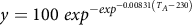
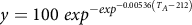
The CWFP data were fit using the Gompertz function, extended to include weed density in the final model (Equation 2), as described by Charles et al. (Reference Charles, Sindel, Cowie and Knox2019a, 2020a):
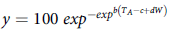 $$y = 100{\rm{\;}}e{xp^{ - ex{p^{b\left( {{T_A} - c + dW} \right)}}}}$$
where y is the relative lint yield; b, c, and d are constants; c+dW is the inflection point of the curve; T A is the time of weed addition; and W is the weed density.
The CTWR data were fit to modified logistic functions including an additional term allowing the lower asymptote of the curves to be above 0% relative yield (Equation 3):
 $$y = a + {\rm{ }}{b \over {1 + ex{p^{c\left( {{T_R} - d} \right)}}}}$$
where y is the relative lint yield, a is the lower asymptote, a+b defines the upper asymptote, c is a constant, T R is the time of weed removal, and d is the inflection point of the curve. The upper asymptote was constrained to 100% relative yield where the model predicted an asymptote below 100%. Models were fit with and without the additional a parameter and the model of best fit was chosen, as indicated by the Akaike information criterion (AIC).
The logistic function was further extended by including the time of weed addition to allow the successive addition events to be included in a combined model, and weed density was also included in the final CTWR model (Equation 4):
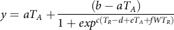 $$y = a{T_A} + {{\left( {b - a{T_A}} \right)} \over {1 + ex{p^{c\left( {{T_R} - d + e{T_A} + fW{T_R}} \right)}}}}$$
where y is the relative lint yield; a, c, d, e, and f are constants; b is the upper asymptote; T A is the time of weed addition; W is the weed density; and T R is the time of weed removal. Models were fit with and without the additional terms and the model of best fit was chosen, as indicated by the AIC.
Results and Discussion
Competition with 20 Common Sunflower Plants Per Square Meter
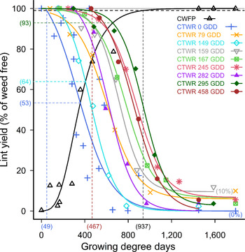
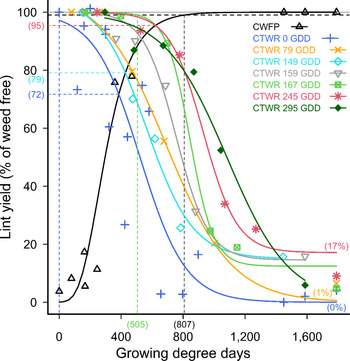
Cotton yields on the weed-free plots averaged 5,178 kg seed cotton ha−1 and 2,041 kg lint ha−1 over the three seasons of the study. Common sunflower plants competed strongly with cotton, with full-season competition causing 100% yield loss with 20 common sunflower plants m−2 (Figure 1). The CPWC commenced at crop emergence, 49 GDD POST, when 20 weeds m−2 were added at the time of crop planting (Figure 1), and continued until mid-season, 937 GDD, similar to the CPWC reported by others (Bukun Reference Bukun2004; Charles et al. Reference Charles, Sindel, Cowie and Knox2019a). The point of minimum yield loss from a single weed-control measure (Webster et al. Reference Webster, Grey, Flanders and Culpepper2009) was 47% from season-long competition (Figure 1). This result was again similar to the findings reported by Charles et al. (Reference Charles, Sindel, Cowie and Knox2019a), but greater than those reported by Bukun (Reference Bukun2004), who used a naturally occurring weed population with staggered weed emergence, when the majority of the weeds emerged more than 5 wk POST. This delay of 5 wk in weed emergence may have contributed to the reduction in competition, as indicated by the higher points of minimum yield loss, reported by Bukun (Reference Bukun2004).
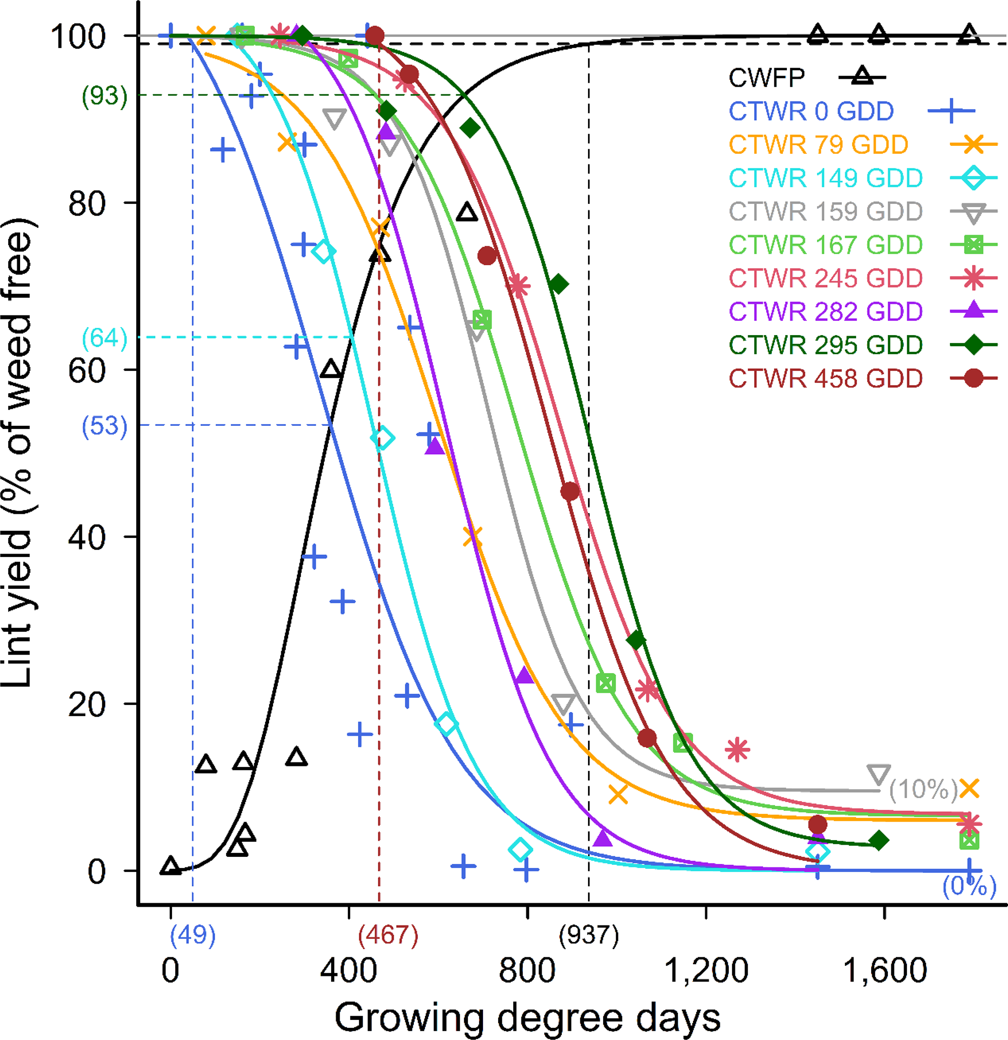
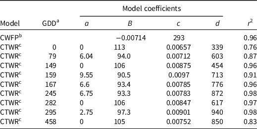
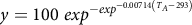
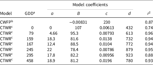
Figure 1. Critical period for weed control (CPWC) for 20 common sunflower plants m−2 competing with cotton. Common sunflower was added at 0, 79, 149, 159, 167, 245, 282, 295, and 458 growing degree days (GDD). Data points are treatment means. Horizontal grey and dashed black lines indicate the weed-free yield and 1% yield-loss threshold, respectively. The intersections of the critical time for weed removal (CTWR) and critical weed-free period (CWFP) lines with the yield-reduction threshold defines the CPWC for each time of weed introduction. Bracketed values on the y-axis and dashed horizontal lines show points of minimum yield loss from a single control input. Bracketed values on the x-axis and dashed vertical lines show the earliest and latest start, and the end of the CPWC. Minimum and maximum yield losses are indicated by bracketed values at the ends of the CTWR curves. The CWFP curve was described by Equation 2:
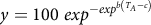
 $$y = 100{\rm{\;}}{exp^{{ - exp^{b\left( {{T_A} - c}\right)}}}}$$
, where y is the relative lint yield, b is a constant, T
A
is the time of weed addition, and c is the inflection point of the curve. The CTWR curve was described by Equation 3: y = a+b/(1+exp
c[T
R
−d]), where y is the relative lint yield, a is the lower asymptote, a+b defines the upper asymptote, c is a constant, T
R
is the time of weed removal, and d is the inflection point of the curve. Coefficients of the models are presented in Table 1.
$$y = 100{\rm{\;}}{exp^{{ - exp^{b\left( {{T_A} - c}\right)}}}}$$
, where y is the relative lint yield, b is a constant, T
A
is the time of weed addition, and c is the inflection point of the curve. The CTWR curve was described by Equation 3: y = a+b/(1+exp
c[T
R
−d]), where y is the relative lint yield, a is the lower asymptote, a+b defines the upper asymptote, c is a constant, T
R
is the time of weed removal, and d is the inflection point of the curve. Coefficients of the models are presented in Table 1.
The relationships for the later weed additions, added 79 GDD to 458 GDD POST (Figure 1), followed similar patterns to the curves for weeds added at the time of crop planting, but with the yield-loss threshold exceeded later in crop life, and with less yield loss, as indicated by the points of minimum yield loss, as reported by Bukun (Reference Bukun2004). The points of minimum yield loss ranged from 7% to 36%, and yield loss from full-season (1,600 GDD) competition ranged from 90% to 100% (Figure 1).
The relationships indicated that the delay between the time of weed addition and the start of the CPWC generally increased as the time of weed addition was delayed, increasing from 49 GDD, to 91 GDD, and 159 GDD after the time of weed addition, with weeds added 0 GDD, 159 GDD, and 295 GDD POST, respectively (Figure 1). However, this pattern was not consistent over all times of weed addition, with shorter delays of 30 GDD and 9 GDD for weeds added at 282 GDD and 458 GDD respectively, compared with 49 GDD for weeds added at 0 GDD (Figure 1).
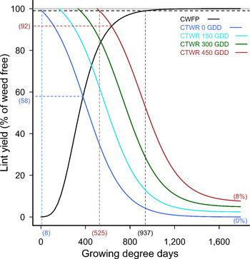
The combined data set was fit to the extended logistic function (Equation 4), resulting in a model including both the time of weed addition and the time of weed removal (Figure 2). This model described the change in the CPWC with later weed additions, up to 450 GDD POST, with reductions in the points of minimum yield loss and increasing delays in the start of the CPWC after delayed weed emergence, and also incremental reductions in the total yield loss at 1,600 GDD when these weeds were not controlled.
Table 1. The critical weed-free period and critical timing for weed control relationships for 20 common sunflower plants per square meter competing with cotton. d
a The time of weed addition in growing degree days.
b
Data fit to Equation 2:
 $$y = 100{\rm{\;}}{exp^{{ - exp^{b\left( {{T_A} - c}\right)}}}}$$
, where y is the relative lint yield, b is a constant, T
A
is the time of weed addition, and c is the inflection point of the curve.
$$y = 100{\rm{\;}}{exp^{{ - exp^{b\left( {{T_A} - c}\right)}}}}$$
, where y is the relative lint yield, b is a constant, T
A
is the time of weed addition, and c is the inflection point of the curve.
c Data fit to Equation 3: y = a+b/(1+exp c[T R −d]), where y is the relative lint yield, a is the lower asymptote, a+b defines the upper asymptote, c is a constant, T R is the time of weed removal, and d is the inflection point of the curve.
d Abbreviations: CTWR, critical timing for weed removal; CWFP, critical weed-free period; GDD, growing degree days.
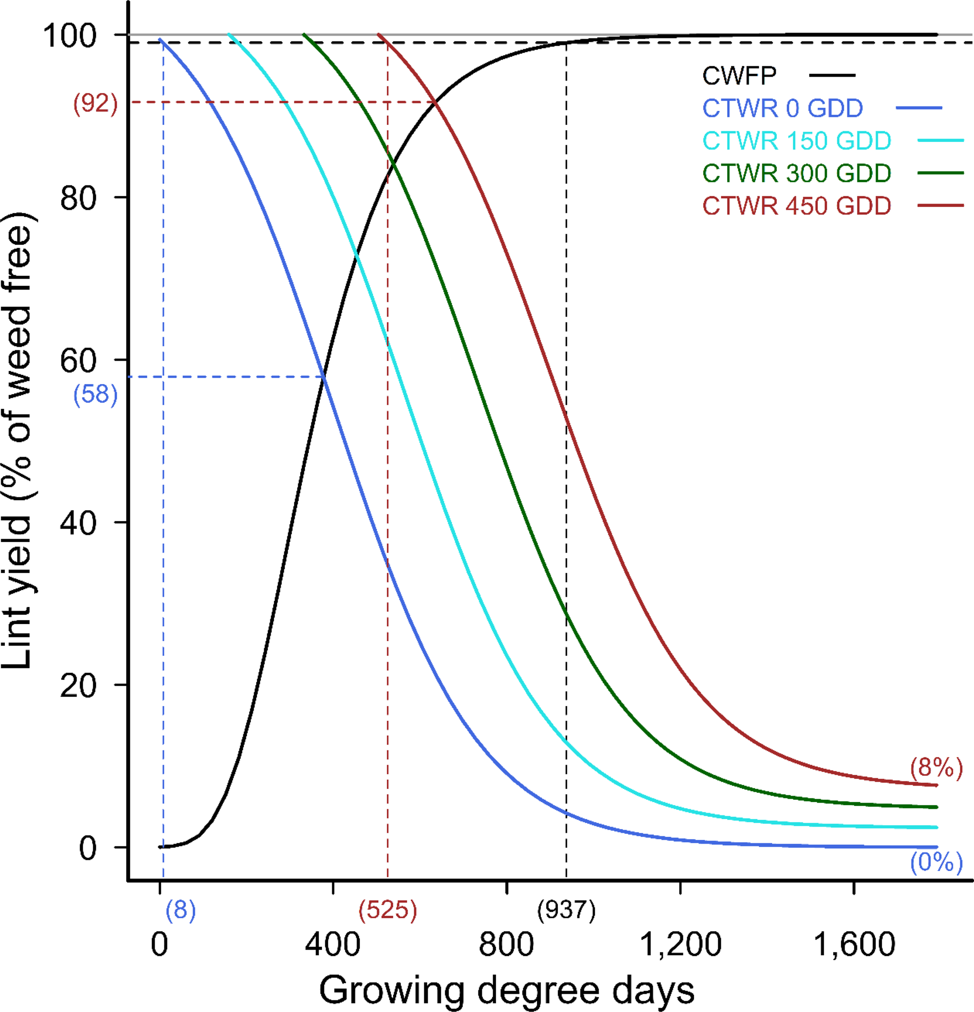
Figure 2. Critical period for weed control (CPWC) for 20 common sunflower plants m−2 competing with cotton, over a range of times of weed addition. The derived relationships for common sunflower plants added at 0, 150, 300, and 450 growing degree days (GDD) are presented as examples. Horizontal grey and dashed black lines indicate the weed-free yield and 1% yield-loss threshold, respectively. The intersections of the critical time for weed removal (CTWR) and critical weed-free period (CWFP) lines with the yield-reduction threshold defines the CPWC for each time of weed introduction. Bracketed values on the y-axis and dashed horizontal lines show points of minimum yield loss from a single control input. Bracketed values on the x-axis and dashed vertical lines show the earliest and latest start, and the end of the CPWC. Minimum and maximum yield losses are indicated by bracketed values at the ends of the CTWR curves. The CWFP curve was described by Equation 2:
 $$y = 100{\rm{\;}}{exp^{{ - exp^{-0.00714\left( {{T_A} - 293}\right)}}}}$$
, r
2
= 0.96. The CTWR curve was described by Equation 4: y = 0.0159T
A
+(109−0.0159T
A
)/(1+exp
0.00598 [T
R
−399−1.12T
A
]), r
2
= 0.8.
$$y = 100{\rm{\;}}{exp^{{ - exp^{-0.00714\left( {{T_A} - 293}\right)}}}}$$
, r
2
= 0.96. The CTWR curve was described by Equation 4: y = 0.0159T
A
+(109−0.0159T
A
)/(1+exp
0.00598 [T
R
−399−1.12T
A
]), r
2
= 0.8.
Competition with 10 Common Sunflower Plants Per Square Meter
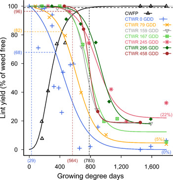
Common sunflower at the lesser density of 10 plants m−2 also competed strongly with cotton, with a yield reduction of 100% from full-season competition when weeds were added at 0 GDD (Figure 3) as previously reported (Charles et al. Reference Charles, Sindel, Cowie and Knox2019a). The CWFP and CTWR relationships with 10 common sunflower plants m−2 followed the same pattern as that for 20 weeds m−2, with the CPWC starting before crop emergence, 29 GDD POST (Figure 3), when weeds were added at the time of crop planting and ended at 783 GDD. However, the lower density of weeds caused less minimum yield loss, with 32% yield loss with 10 weeds m−2 introduced at crop planting (Figure 3), compared with 47% with 20 weeds m−2 (Figure 1).
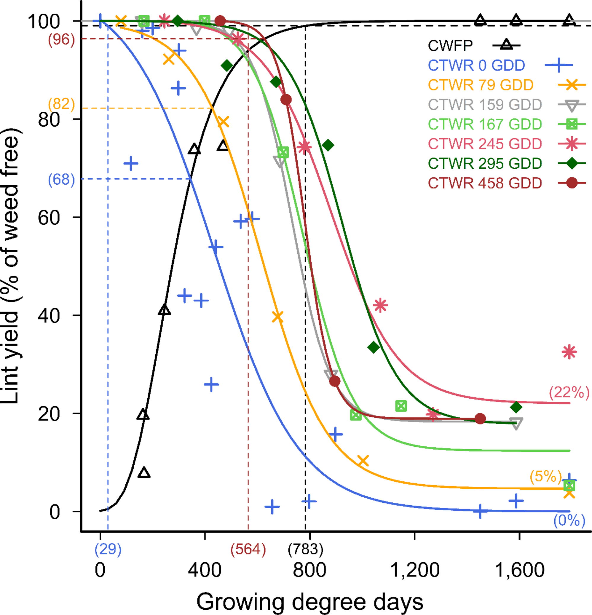
Figure 3. Critical period for weed control (CPWC) for 10 common sunflower plants m−2 competing with cotton. Common sunflower was added at 0, 79, 159, 167, 245, 295, and 458 growing degree days (GDD). Data points are treatment means. Horizontal grey and dashed black lines indicate the weed-free yield and 1% yield-loss threshold, respectively. The intersections of the critical time for weed removal (CTWR) and critical weed-free period (CWFP) lines with the yield-reduction threshold defines the CPWC for each time of weed introduction. Bracketed values on the y-axis and dashed horizontal lines show points of minimum yield loss from a single control input. Bracketed values on the x-axis and dashed vertical lines show the earliest and latest start, and the end of the CPWC. Minimum and maximum yield losses are indicated by bracketed values at the ends of the CTWR curves. The CWFP curve was described by Equation 2:
 $$y = 100{\rm{\;}}{exp^{{ - exp^{b\left( {{T_A} - c}\right)}}}}$$
, where y is the relative lint yield, b is a constant, T
A
is the time of weed addition, and c is the inflection point of the curve. The CTWR curve was described by Equation 3: y = a+b/(1+exp
c[T
R
−d]), where y is the relative lint yield, a is the lower asymptote, a+b defines the upper asymptote, c is a constant, T
R
is the time of weed removal, and d is the inflection point of the curve. Coefficients of the models are presented in Table 2.
$$y = 100{\rm{\;}}{exp^{{ - exp^{b\left( {{T_A} - c}\right)}}}}$$
, where y is the relative lint yield, b is a constant, T
A
is the time of weed addition, and c is the inflection point of the curve. The CTWR curve was described by Equation 3: y = a+b/(1+exp
c[T
R
−d]), where y is the relative lint yield, a is the lower asymptote, a+b defines the upper asymptote, c is a constant, T
R
is the time of weed removal, and d is the inflection point of the curve. Coefficients of the models are presented in Table 2.
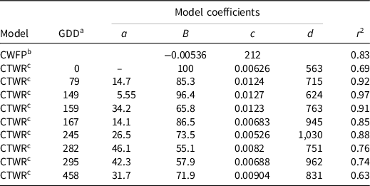
The relationships for the later weed additions again followed similar patterns to the curves for weeds added at planting, and for the curves for 20 weeds m−2 but with reduced yield losses. The points of minimum yield loss from a single weed control input ranged from 4% to 18% for 10 weeds m−2 added 79 GDD to 458 GDD POST (Figure 3), compared with losses of 7% to 36% with 20 weeds m−2. Season-long competition from the later weed additions resulted in 78% to 95% yield loss with 10 weeds m−2 added at 79 GDD to 458 GDD POST, compared with the 90% to 100% yield loss with 20 weeds m−2. Full-season yield loss predicted by the combined model reduced from 100% yield loss with weeds added at crop planting, to 89%, 79%, and 68% yield loss with weeds added 150, 300, and 450 POST, respectively (Figure 4).
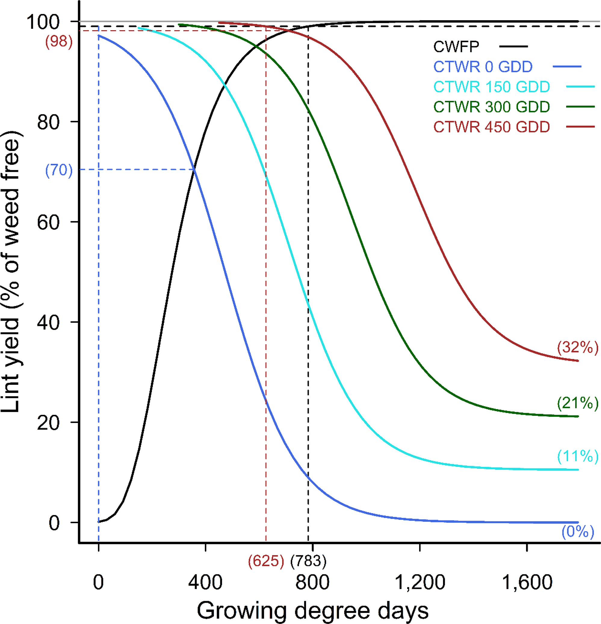
Figure 4. Critical period for weed control (CPWC) for 10 common sunflower plants m−2 competing with cotton, over a range of times of weed addition. The derived relationships for common sunflower plants added at 0, 150, 300, and 450 growing degree days (GDD) are presented as examples. Horizontal grey and dashed black lines indicate the weed-free yield and 1% yield-loss threshold, respectively. The intersections of the critical time for weed removal (CTWR) and critical weed-free period (CWFP) lines with the yield-reduction threshold defines the CPWC for each time of weed introduction. Bracketed values on the y-axis and dashed horizontal lines show points of minimum yield loss from a single control input. Bracketed values on the x-axis and dashed vertical lines show the earliest and latest start, and the end of the CPWC. Minimum and maximum yield losses are indicated by bracketed values at the ends of the CTWR curves. The CWFP curve was described by Equation 2:
 $$y = 100{\rm{\;}}{exp^{{ - exp^{ - 0.00831\left( {{T_A} - 230}\right)}}}}$$
, r
2
= 0.87. The CTWR curve was described by Equation 4: y = 0.0701T
A
+(100−0.0701T
A
)/(1+exp
0.00748 [T
R
−473−1.59T
A
]), r
2
= 0.83.
$$y = 100{\rm{\;}}{exp^{{ - exp^{ - 0.00831\left( {{T_A} - 230}\right)}}}}$$
, r
2
= 0.87. The CTWR curve was described by Equation 4: y = 0.0701T
A
+(100−0.0701T
A
)/(1+exp
0.00748 [T
R
−473−1.59T
A
]), r
2
= 0.83.
Competition with Two and Five Common Sunflower Plants Per Square Meter
The effects on cotton yield of competition from 2 and 5 common sunflower plants m−2 followed the trends of the higher weed densities, with the point of minimum yield loss ranging from 5% to 28% with 5 plants m−2 (Figure 5), and 7% to 28% with 2 plants m−2 (Figure 6). Season-long competition from weeds introduced at crop planting remained at or close to 100% yield loss over these lower weed densities (Figures 5 and 6), but season-long competition from the later weeds additions resulted in 54% to 94% yield loss with 2 weeds m−2 (Figure 6), less than was observed with the higher weed densities.
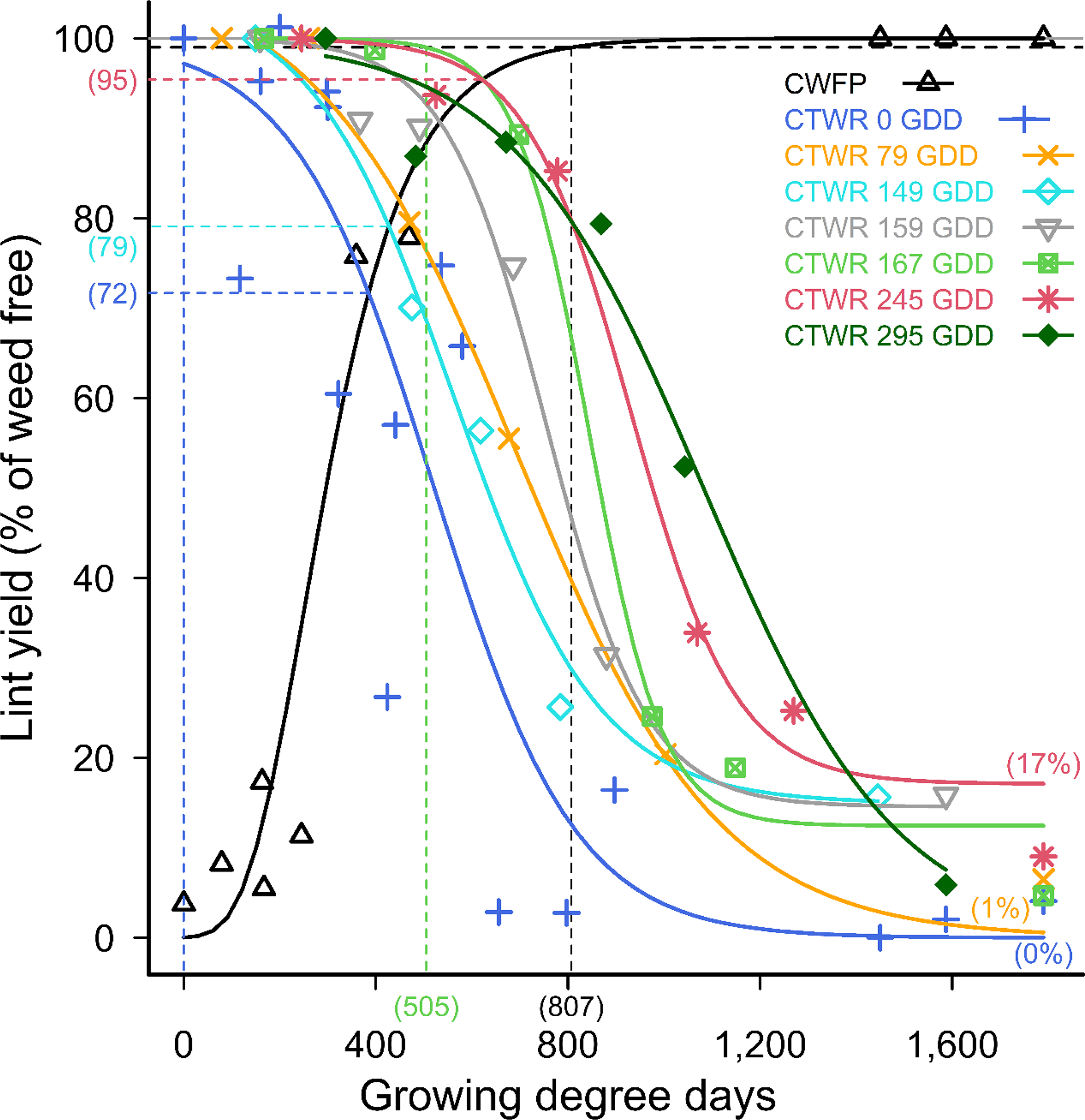
Figure 5. Critical period for weed control (CPWC) for 5 common sunflower plants m−2 competing with cotton. Common sunflower was added at 0, 79, 149, 159, 167, 245, and 295 growing degree days (GDD). Data points are treatment means. Horizontal grey and dashed black lines indicate the weed-free yield and 1% yield-loss threshold, respectively. The intersections of the critical time for weed removal (CTWR) and critical weed-free period (CWFP) lines with the yield-reduction threshold defines the CPWC for each time of weed introduction. Bracketed values on the y-axis and dashed horizontal lines show points of minimum yield loss from a single control input. Bracketed values on the x-axis and dashed vertical lines show the earliest and latest start, and the end of the CPWC. Minimum and maximum yield losses are indicated by bracketed values at the ends of the CTWR curves. The CWFP curve was described by Equation 2:
 $$y = 100{\rm{\;}}{exp^{{ - exp^{b\left( {{T_A} - c}\right)}}}}$$
, where y is the relative lint yield, b is a constant, T
A
is the time of weed addition, and c is the inflection point of the curve. The CTWR curve was described by Equation 3: y = a+b/(1+exp
c[T
R
−d]), where y is the relative lint yield, a is the lower asymptote, a+b defines the upper asymptote, c is a constant, T
R
is the time of weed removal, and d is the inflection point of the curve. Coefficients of the models are presented in Table 3.
$$y = 100{\rm{\;}}{exp^{{ - exp^{b\left( {{T_A} - c}\right)}}}}$$
, where y is the relative lint yield, b is a constant, T
A
is the time of weed addition, and c is the inflection point of the curve. The CTWR curve was described by Equation 3: y = a+b/(1+exp
c[T
R
−d]), where y is the relative lint yield, a is the lower asymptote, a+b defines the upper asymptote, c is a constant, T
R
is the time of weed removal, and d is the inflection point of the curve. Coefficients of the models are presented in Table 3.
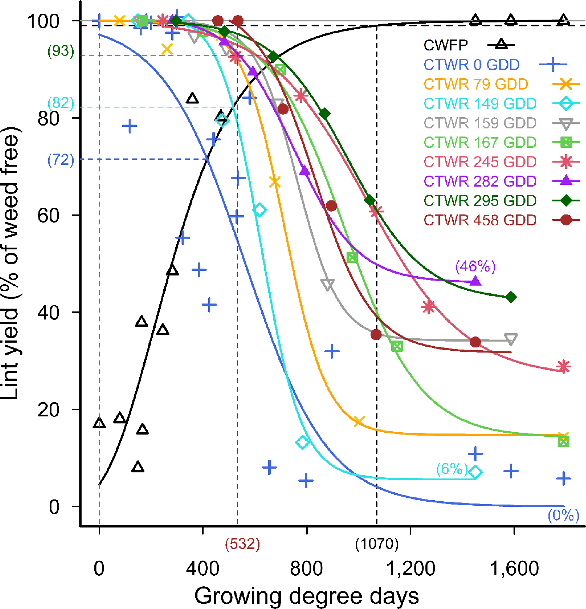
Figure 6. Critical period for weed control (CPWC) for 2 common sunflower plants m−2 competing with cotton. Common sunflower was added at 0, 79, 149, 159, 167, 245, 282, 295, and 458 growing degree days (GDD). Data points are treatment means. Horizontal grey and dashed black lines indicate the weed-free yield and 1% yield-loss threshold, respectively. The intersections of the critical time for weed removal (CTWR) and critical weed-free period (CWFP) lines with the yield-reduction threshold defines the CPWC for each time of weed introduction. Bracketed values on the y-axis and dashed horizontal lines show points of minimum yield loss from a single control input. Bracketed values on the x-axis and dashed vertical lines show the earliest and latest start, and the end of the CPWC. Minimum and maximum yield losses are indicated by bracketed values at the ends of the CTWR curves. The CWFP curve was described by Equation 2:
 $$y = 100{\rm{\;}}{exp^{{ - exp^{b\left( {{T_A} - c}\right)}}}}$$
, where y is the relative lint yield, b is a constant, T
A
is the time of weed addition, and c is the inflection point of the curve. The CTWR curve was described by Equation 3: y = a+b/(1+exp
c[T
R
−d]), where y is the relative lint yield, a is the lower asymptote, a+b defines the upper asymptote, c is a constant, T
R
is the time of weed removal, and d is the inflection point of the curve. Coefficients of the models are presented in Table 4.
$$y = 100{\rm{\;}}{exp^{{ - exp^{b\left( {{T_A} - c}\right)}}}}$$
, where y is the relative lint yield, b is a constant, T
A
is the time of weed addition, and c is the inflection point of the curve. The CTWR curve was described by Equation 3: y = a+b/(1+exp
c[T
R
−d]), where y is the relative lint yield, a is the lower asymptote, a+b defines the upper asymptote, c is a constant, T
R
is the time of weed removal, and d is the inflection point of the curve. Coefficients of the models are presented in Table 4.
Full-season yield loss predicted by the combined model with competition from 5 common sunflower plants m−2 reduced from 100% with weeds added at crop planting, to 91%, and 82% yield loss with weeds added 150 and 300 GDD POST, respectively (Figure 7). Full-season yield loss for competition from 2 common sunflower plants m−2 reduced from 100% with weeds added at crop planting, to 83%, 64%, and 49% yield loss with weeds added 150, 300, and 450 GDD POST, respectively (Figure 8). The models predicted 100% yield loss from full-season competition from all densities of weeds that emerged with the crop (Figures 2, 4, 7, and 8).
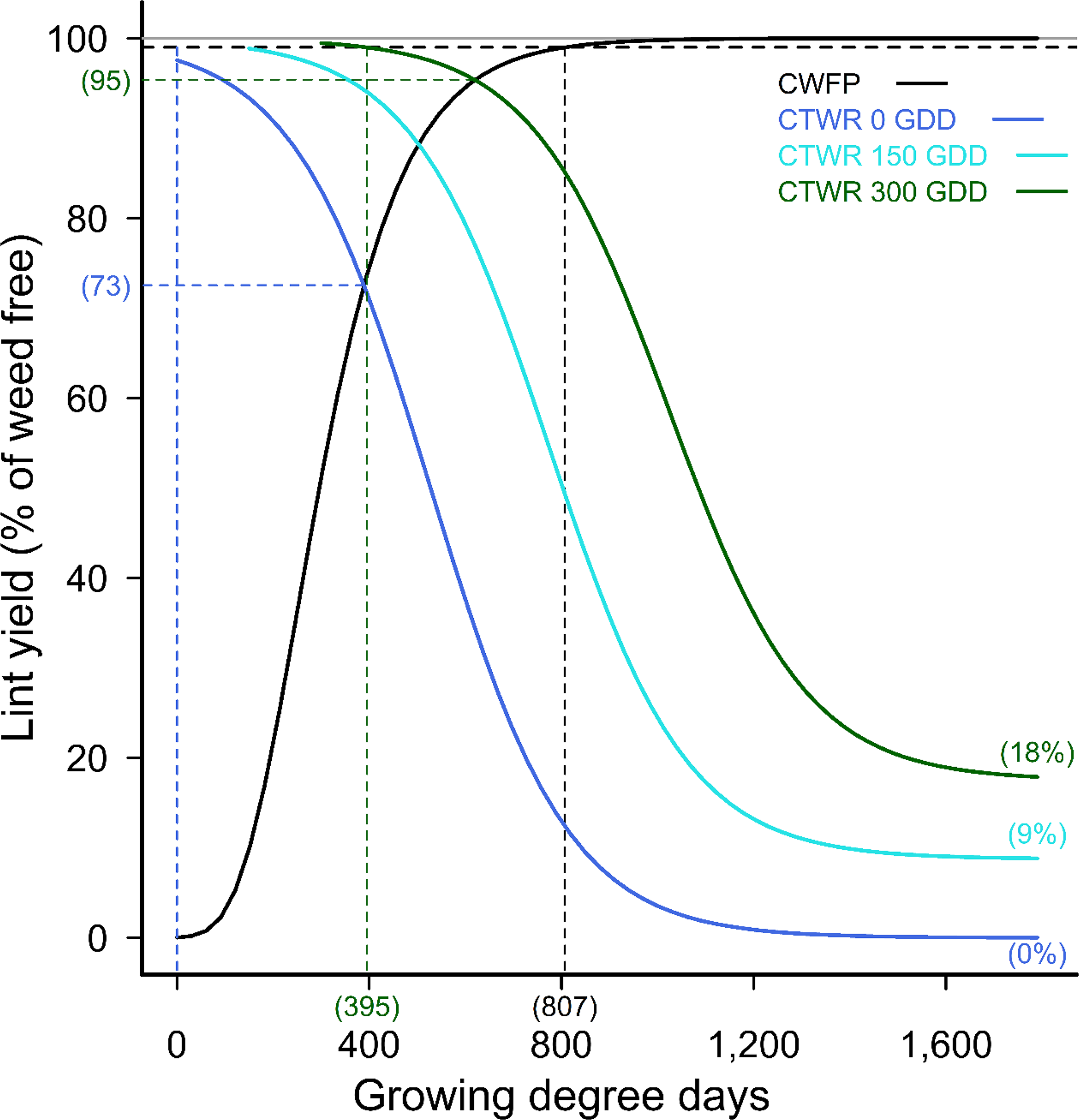
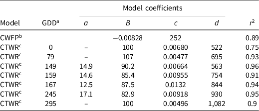
Figure 7. Critical period for weed control (CPWC) for 5 common sunflower plants m−2 competing with cotton, over a range of times of weed addition. The derived relationships for common sunflower plants added at 0, 150, and 300 growing degree days (GDD) are presented as examples. Horizontal grey and dashed black lines indicate the weed-free yield and 1% yield-loss threshold, respectively. The intersections of the critical time for weed removal (CTWR) and critical weed-free period (CWFP) lines with the yield-reduction threshold defines the CPWC for each time of weed introduction. Bracketed values on the y-axis and dashed horizontal lines show points of minimum yield loss from a single control input. Bracketed values on the x-axis and dashed vertical lines show the earliest and latest start, and the end of the CPWC. Minimum and maximum yield losses are indicated by bracketed values at the ends of the CTWR curves. The CWFP curve was described by Equation 2:
 $$y = 100{\rm{\;}}{exp^{{ - exp^{ - 0.00828\left( {{T_A} - 252}\right)}}}}$$
, r
2
= 0.89. The CTWR curve was described by Equation 4: y = 0.0584T
A
+(100−0.0584T
A
)/(1+exp
0.007 [T
R
−528−1.65T
A
]), r
2
= 0.84.
$$y = 100{\rm{\;}}{exp^{{ - exp^{ - 0.00828\left( {{T_A} - 252}\right)}}}}$$
, r
2
= 0.89. The CTWR curve was described by Equation 4: y = 0.0584T
A
+(100−0.0584T
A
)/(1+exp
0.007 [T
R
−528−1.65T
A
]), r
2
= 0.84.

Figure 8. Critical period for weed control (CPWC) for 2 common sunflower plants m−2 competing with cotton, over a range of times of weed addition. The derived relationships for common sunflower plants added at 0, 150, 300, and 450 growing degree days (GDD) are presented as examples. Horizontal grey and dashed black lines indicate the weed-free yield and 1% yield-loss threshold, respectively. The intersections of the critical time for weed removal (CTWR) and critical weed-free period (CWFP) lines with the yield-reduction threshold defines the CPWC for each time of weed introduction. Bracketed values on the y-axis and dashed horizontal lines show points of minimum yield loss from a single control input. Bracketed values on the x-axis and dashed vertical lines show the earliest and latest start, and the end of the CPWC. Minimum and maximum yield losses are indicated by bracketed values at the ends of the CTWR curves. The CWFP curve was described by Equation 2:
 $$y = 100{\rm{\;}}{exp^{{ - exp^{ - 0.00536\left( {{T_A} - 212}\right)}}}}$$
, r
2
= 0.83. The CTWR curve was described by Equation 4: y = 0.11T
A
+(103−0.11T
A
)/(1+exp
0.00522 [T
R
−607−1.02T
A
]), r
2
= 0.71.
$$y = 100{\rm{\;}}{exp^{{ - exp^{ - 0.00536\left( {{T_A} - 212}\right)}}}}$$
, r
2
= 0.83. The CTWR curve was described by Equation 4: y = 0.11T
A
+(103−0.11T
A
)/(1+exp
0.00522 [T
R
−607−1.02T
A
]), r
2
= 0.71.
Developing a Combined Competition Model that Includes Weed Density
Data sets from the weed densities of 2, 5, 10, and 20 common sunflower plants m−2 were combined and fit to extended CPWC relationships, including weed density in the models (Charles et al. Reference Charles, Sindel, Cowie and Knox2019a). Additional terms were included in the CTWR model (Equation 4) allowing this model to have a lower asymptote above 0% lint yield. These models give the predicted yield loss from densities of 2 to 20 common sunflower plants m−2, for weeds introduced 0 GDD to 450 GDD POST, with examples of these extremes shown in Figure 9. The yield loss from season-long competition ranged from 100% loss with all weed densities introduced at crop planting, through to 42% to 57% yield loss with 2 to 20 weeds m−2, introduced 450 GDD POST (Figure 9). The point of minimum yield loss was affected by both weed density and the time of weed addition, ranging from 48% yield loss with 20 weeds m−2 introduced at planting, through to 1.1% yield loss with two weeds introduced 450 GDD POST.
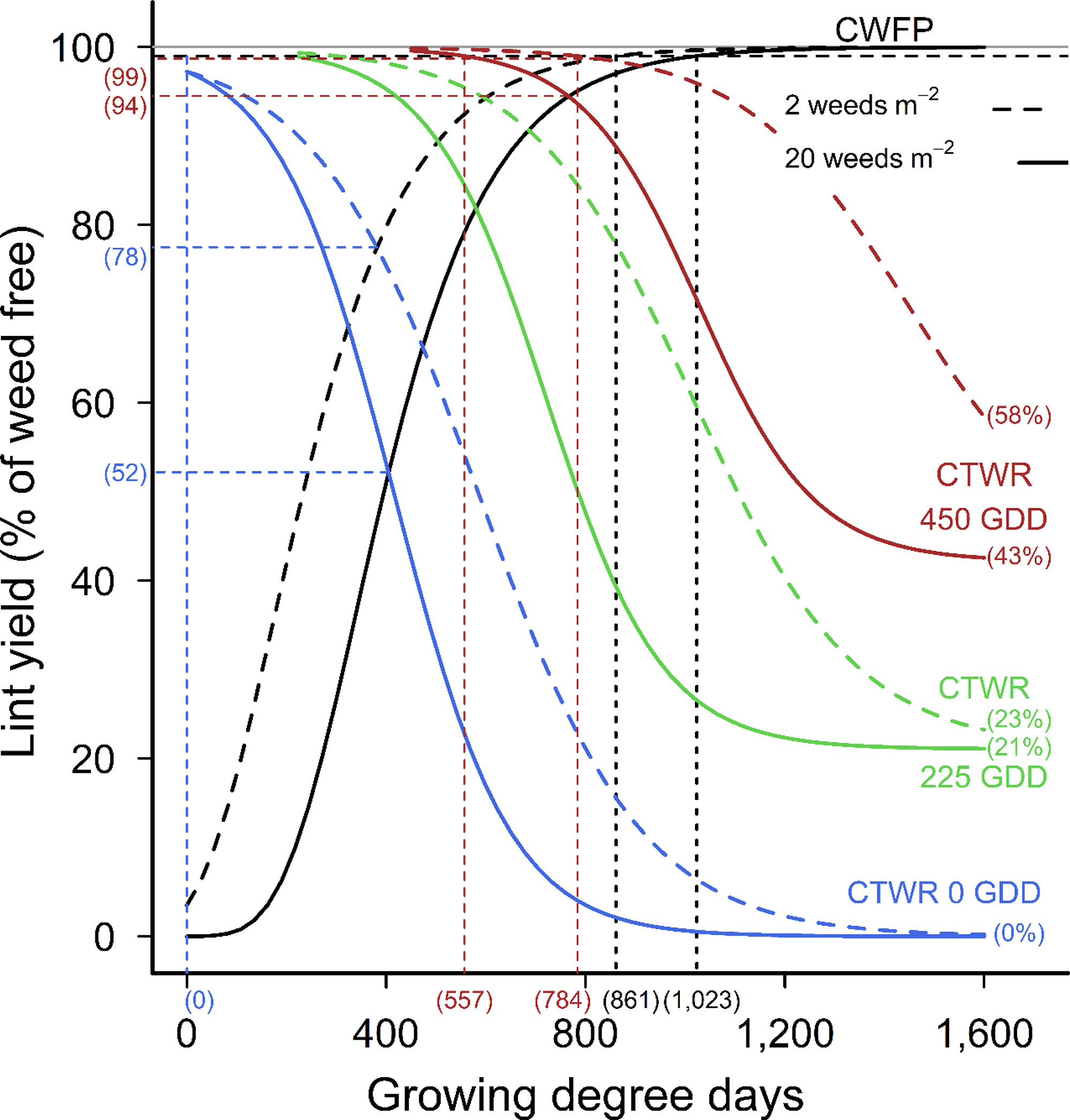
Figure 9. The critical period for weed control (CPWC) for common sunflower competing with cotton, over a range of times of weed addition and weed densities. The derived relationships for common sunflower added at 0, 225, and 450 growing degree days (GDD) after crop planting, with densities of 2, and 20 plants m−2 are presented as examples for the critical timing for weed removal (CTWR) and critical weed free period (CWFP) relationships. Equations for the relationships are y = 0.0937T
A
+(100−0.0937T
A
)/(1+exp0.00583[T
R
−612−2.01T
A
+0.0237W*T
R
]), r
2
= 0.68; and
 $$y = 100{\rm{\;}}{exp^{{ - exp^{ - 0.00675\left( {{T_A} - 161 - 9W}\right)}}}}$$
, r
2
= 0.86; respectively. Parameters of the curves are as follows: y is the relative lint yield; T
A
is the time of weed addition; T
R
is the time of weed removal; and W is the weed density. Horizontal grey and dashed black lines indicate the weed-free yield and 1% yield-loss threshold, respectively. The intersections of the CTWR and CWFP relationships with the yield-reduction threshold defines the CPWC for each weed density and time of weed introduction. The intersections of these lines are indicated by dashed vertical lines and bracketed values. The points of minimum yield loss are indicated by dashed horizontal lines and bracketed values, and the maximum yield losses are shown by bracketed values.
$$y = 100{\rm{\;}}{exp^{{ - exp^{ - 0.00675\left( {{T_A} - 161 - 9W}\right)}}}}$$
, r
2
= 0.86; respectively. Parameters of the curves are as follows: y is the relative lint yield; T
A
is the time of weed addition; T
R
is the time of weed removal; and W is the weed density. Horizontal grey and dashed black lines indicate the weed-free yield and 1% yield-loss threshold, respectively. The intersections of the CTWR and CWFP relationships with the yield-reduction threshold defines the CPWC for each weed density and time of weed introduction. The intersections of these lines are indicated by dashed vertical lines and bracketed values. The points of minimum yield loss are indicated by dashed horizontal lines and bracketed values, and the maximum yield losses are shown by bracketed values.
Table 2. The critical weed-free period and critical timing for weed control relationships for 10 common sunflower plants per square meter competing with cotton. d
a The time of weed addition in growing degree days.
b
Data fit to Equation 2:
 $$y = 100{\rm{\;}}{exp^{{ - exp^{b\left( {{T_A} - c}\right)}}}}$$
, where y is the relative lint yield, b is a constant, T
A
is the time of weed addition, and c is the inflection point of the curve.
$$y = 100{\rm{\;}}{exp^{{ - exp^{b\left( {{T_A} - c}\right)}}}}$$
, where y is the relative lint yield, b is a constant, T
A
is the time of weed addition, and c is the inflection point of the curve.
c Data fit to Equation 3: y = a+b/(1+exp c[T R −d]), where y is the relative lint yield, a is the lower asymptote, a+b defines the upper asymptote, c is a constant, T R is the time of weed removal, and d is the inflection point of the curve.
d Abbreviations: CTWR, critical timing for weed removal; CWFP, critical weed-free period; GDD, growing degree days.
The CPWC predicted by the extended models commenced at the time of weed addition for all weed densities when weeds emerged with the crop, and continued until 861 GDD and 1,023 GDD, with 2 and 20 common sunflower plants m−2 competing with cotton, respectively. The CPWC began at the time of weed addition for weeds introduced at crop planting and continued to be at the time of weed addition for weeds introduced up until 156 GDD POST with 2 weeds m −2 , and 247 GDD POST with 20 weeds m−2. There was an increasing delay between the time of weed introduction and the start of the CPWC beyond these points. For weeds introduced at 450 GDD, the CPWC did not start until 557 GDD and 785 GDD, for 20 and 2 weeds m−2, respectively (Figure 9).
Table 3. The critical weed-free period and critical timing for weed control relationships for five common sunflower plants per square meter competing with cotton. d
a The time of weed addition in growing degree days.
b
Data fit to Equation 2:
 $$y = 100{\rm{\;}}{exp^{{ - exp^{b\left( {{T_A} - c}\right)}}}}$$
, where y is the relative lint yield, b is a constant, T
A
is the time of weed addition, and c is the inflection point of the curve.
$$y = 100{\rm{\;}}{exp^{{ - exp^{b\left( {{T_A} - c}\right)}}}}$$
, where y is the relative lint yield, b is a constant, T
A
is the time of weed addition, and c is the inflection point of the curve.
c Data fit to Equation 3: y = a+b/(1+exp c[T R −d]), where y is the relative lint yield, a is the lower asymptote, a+b defines the upper asymptote, c is a constant, T R is the time of weed removal, and d is the inflection point of the curve.
d Abbreviations: CTWR, critical timing for weed removal; CWFP, critical weed-free period; GDD, growing degree days.
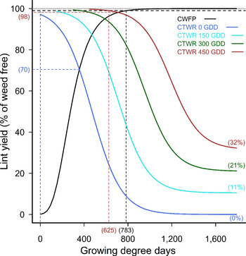
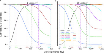
Extrapolation of our data would suggest that weeds that emerged even later in the season, but still within the CPWC, may not need to be controlled until after the end of the CPWC. To test our model’s prediction of the competitive impact of weeds that emerge late in the CPWC, we extended the fit of our CPWC model for 2 common sunflower plants m−2 from 0 GDD through to 800 GDD (Figure 10A), and for 20 common sunflower plants m−2 from 0 GDD through 1,000 GDD (Figure 10B). Our model predicts that if 2 common sunflower plants m−2 emerge at 800 GDD (61 GDD before the end of the CPWC), they will not need to be controlled until 1,596 GDD (Figure 10A); that is, they will not grow to sufficient size to cause yield loss exceeding the yield-loss threshold until 1,596 GDD. Twenty common sunflower plants per square meter emerging at 1,000 GDD (23 GDD before the end of the CPWC) would not need to be controlled until 1,581 GDD (Figure 10B).
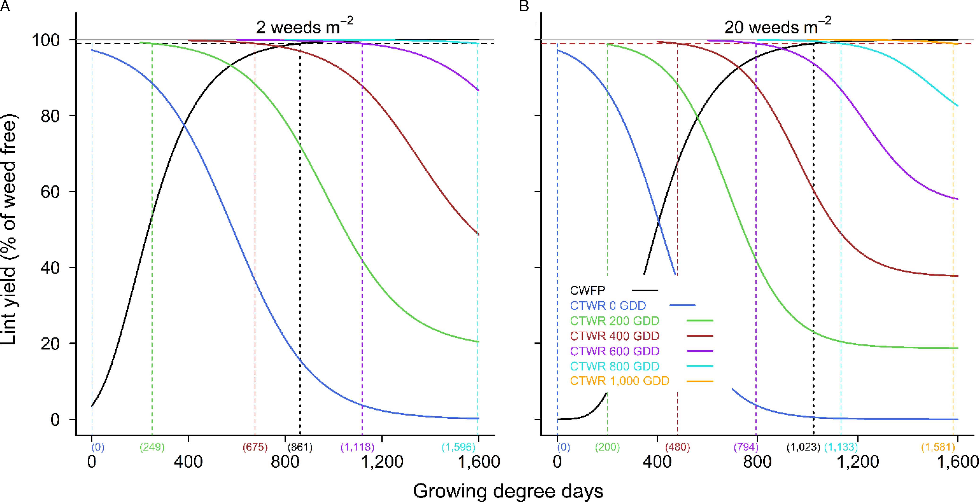
Figure 10. The critical period for weed control (CPWC) for 2 (A) and 20 (B) common sunflower plants m−2 competing with cotton, over a range of times of weed addition and weed densities. The derived relationships for common sunflower added at 0, 200, 400, 600, 800, and 1,000 growing degree days (GDD) after crop planting are presented as examples for the critical timing for weed removal (CTWR) and critical weed free period (CWFP) relationships. Equations for the relationships are y = 0.0937T
A
+(100−0.0937T
A
)/ (1+exp0.00583(T
R
−612−2.01T
A
+0.0237W*T
R
)), r
2
= 0.68; and
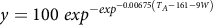 $$y = 100{\rm{\;}}{exp^{{ - exp^{ - 0.00675\left( {{T_A} - 161 - 9W}\right)}}}}$$
, r
2
= 0.86, respectively. Parameters of the curves are as follows: y is the relative lint yield; T
A
is the time of weed addition; T
R
is the time of weed removal; and W is the weed density. Horizontal grey and dashed black lines indicate the weed-free yield and 1% yield-loss threshold, respectively. The intersections of the CTWR and CWFP relationships with the yield-loss threshold are indicated by dashed vertical lines and bracketed values, showing the start and end of the CPWC.
$$y = 100{\rm{\;}}{exp^{{ - exp^{ - 0.00675\left( {{T_A} - 161 - 9W}\right)}}}}$$
, r
2
= 0.86, respectively. Parameters of the curves are as follows: y is the relative lint yield; T
A
is the time of weed addition; T
R
is the time of weed removal; and W is the weed density. Horizontal grey and dashed black lines indicate the weed-free yield and 1% yield-loss threshold, respectively. The intersections of the CTWR and CWFP relationships with the yield-loss threshold are indicated by dashed vertical lines and bracketed values, showing the start and end of the CPWC.
Thus we conclude that for weeds emerging with the crop, the CPWC defines the time at which weeds must be controlled to prevent yield loss exceeding the threshold. However, weeds that emerge during the CPWC must be controlled to prevent yield loss exceeding the threshold, but that this control may not be required until after the CPWC has finished. Whereas this conclusion contradicts the accepted concept of the CPWC (Knezevic and Datt Reference Knezevic and Datta2015; Korres and Norsworthy Reference Korres and Norsworthy2015; Price et al. Reference Price, Korres, Norsworthy and Li2018), it is logical that a weed that emerges, say a day before the end of the CPWC, will not grow to be sufficiently large for its competitive effect to exceed the yield-reduction threshold until well after the end of the CPWC. Hence, weeds that emerge during the CPWC will not necessarily need to be controlled during the CPWC, but will need to be controlled before the crop reaches maturity.
Consequently, the CPWC is not the critical period during which weeds must be controlled to prevent yield loss exceeding the yield-loss threshold (Knezevic and Datt Reference Knezevic and Datta2015; Korres and Norsworthy Reference Korres and Norsworthy2015; Price et al. Reference Price, Korres, Norsworthy and Li2018), but that weeds present during the CPWC must be controlled to prevent yield loss. When weeds emerge late in the CPWC, control may not be needed until after the end of the CPWC, but weeds that emerge after the CPWC will not need to be controlled to prevent yield loss exceeding the yield-loss threshold (Zimdahl Reference Zimdahl1988). This conclusion contradicts the traditional view of the CPWC but is logical when considering competition from weeds that emerge late in the CPWC.
Table 4. The critical weed-free period and critical timing for weed control relationships for two common sunflower plants per square meter competing with cotton. d
a The time of weed addition in growing degree days.
b
Data fit to Equation 2:
 $$y = 100{\rm{\;}}{exp^{{ - exp^{b\left( {{T_A} - c}\right)}}}}$$
, where y is the relative lint yield, b is a constant, T
A
is the time of weed addition, and c is the inflection point of the curve.
$$y = 100{\rm{\;}}{exp^{{ - exp^{b\left( {{T_A} - c}\right)}}}}$$
, where y is the relative lint yield, b is a constant, T
A
is the time of weed addition, and c is the inflection point of the curve.
c Data fit to Equation 3: y = a+b/(1+exp c[T R −d]), where y is the relative lint yield, a is the lower asymptote, a+b defines the upper asymptote, c is a constant, T R is the time of weed removal, and d is the inflection point of the curve.
d Abbreviations: CTWR, critical timing for weed removal; CWFP, critical weed-free period; GDD, growing degree days.
Practical Implications
The CPWC remains a valuable tool for enabling weed managers to identify the period of the cropping season during which weed emergence of a sufficient density necessitates the need for weed control to protect crop yields. Application of our extended CPWC relationship to weed management in high-yielding cotton will enable cotton growers to understand the impact of later weed germinations and to identify the time by which these weeds need to be controlled to avoid yield losses exceeding the cost of weed control. Applying a weed control input at or soon after the end of the CPWC would be a practical way of managing late-emerging weeds when these weeds are present at or above threshold levels late in the CPWC and their control is not needed until some point after the end of the CPWC. When this input might occur after crop canopy closure, it may be best to initiate the input as late as possible, but before canopy closure, especially where interrow cultivation is the chosen tool for weed control. Weeds that emerge after this time will still need to be controlled before they set seed to protect the quality of cotton lint, to avoid difficulties with large weeds at harvest, and to manage herbicide resistance by reducing the weed seedbank over time (Charles et al. Reference Charles, Sindel, Cowie and Knox2019a; Korres and Norsworthy Reference Korres and Norsworthy2015). Thus the findings of our research with a large broadleaf weed with 2 to 20 plants m−2 support the traditional practice of applying herbicides and/or interrow cultivation just before crop canopy closure as a cost-effective approach for managing mid- to late-season weeds in cotton.
Acknowledgments
This work was supported by the New South Wales Department of Primary Industries, Cotton Research and Development Corporation, and Australian Cotton Cooperative Research Centre. We thank the many support staff who contributed to the field work and the reviewers of the paper. No conflicts of interest have been declared.


 Open access