1. Introduction and motivation

Building regression models for insurance claims poses several challenges. The process can be particularly difficult for individual insurance policies where a large proportion of claims are zeros, and for those policies with a claim, the losses typically exhibit skewness. The degree of skewness in the positive loss distribution varies widely for different types of insurance products. For example, within a class of automobile insurance policies, the losses arising from damages to the property may be medium-tailed but those arising from liability-related claims may be long-tailed. For short-term insurance contracts, the number of claims is referred to as the claim frequency, while the amount of claims, conditional on the occurrence of a claim, is the claim severity. The information that covariates, or explanatory variables, bring to each component in a regression context allows to capture the possible heterogeneity of the individual policies. These two components are used as predictive models for pure premiums, expected loss costs, and aggregate or total claims in an insurance portfolio.

There is a long history of studying insurance claims based on the two-part framework. Several well-known families of distributions for claim frequencies and claim severities are well documented in [Reference Klugman, Panjer and Willmot15]. As more observed data became increasingly available, additional complexities to traditional regression linear models have been introduced in the literature and in practice; for example, the use of zero-inflated or hurdle models has been discussed to accommodate the shortcomings of traditional models for excess zeros. Interestingly, the Tweedie generalized linear model (GLM) for insurance claims has been particularly popular because it is adaptable to a mixture of zeros and nonnegative insurance claims. Smyth & Jørgensen [Reference Smyth and Jørgensen23] described the Tweedie compound Poisson regression models and calibrated such models using a Swedish third-party insurance claims dataset; the models were fitted to examine dispersion within the GLM framework. The Tweedie distribution can be regarded as a reparameterization of the compound Poisson–gamma distribution, so that model calibration can be done within the GLM framework. Xacur & Garrido [Reference Xacur and Garrido25] compared these two approaches and concluded that there is no clear superior method; the paper also discussed the advantages and disadvantages of the two methods. The Tweedie GLM presents a larger pure premium and implies both a higher claim frequency and claim severity due to the constant scale (dispersion) parameter; in other words, the mean increases with the variance. The constant scale parameter also forces an artificial relationship between claim frequency and claim severity. The Tweedie GLM does not have an optimal coefficient, especially under the inflexible distribution assumption, and it leads to a loss of information because it ignores the number of claims. On the other hand, the Tweedie GLM has fewer parameters to estimate and is thus considered more parsimonious than a two-part framework. When insurance claim data contain small losses due to low frequencies, the two-part framework is likely to overlook the internal connection between the low frequency and the subsequent small loss amount. For example, the frequency model often indicates zero number of claims for small claim policies, which leads to a zero loss prediction. Other works related to the Tweedie GLM can be found in [Reference Frees, Derrig and Meyers5] and [Reference Jørgensen14].

Within the GLM framework, the claim frequency component may not accurately accommodate imbalances caused by the large proportion of zero claims. Simultaneously, a significant limitation is that the regression structure of the logarithmic mean is restricted to a linear form, which may be too inflexible for real applications. With the rapid expansion of the available data for improved decision-making, there is a growing appetite in the insurance industry to expand its tool kit for data analysis and modeling. However, the industry is unarguably highly regulated, so there is pressure for actuaries and data scientists to provide adequate transparency in modeling techniques and results. To find a balance between modeling flexibility and interpretation, in this paper, we propose a parametric model empowered by tree-based methods with a hybrid structure.

Since [Reference Breiman, Friedman, Olshen and Stone1] introduced the Classification and Regression Tree (CART) algorithm, tree-based models have gained momentum as a powerful machine learning approach to decision-making in several disciplines. In particular, single-tree models, such as the CART algorithm, can be interpreted straightforwardly by visualizing the tree structure. The CART algorithm involves separating the explanatory variable space into several mutually exclusive regions and thus creating a nested hierarchy of branches resembling a tree structure. Each separation or branch is referred to as a node. Each of the bottom nodes of the decision tree, called terminal nodes, has a unique path for observable data to enter the region. Once the decision tree is constructed, it is possible to predict and locate the terminal node for scoring the dataset using a new set of observed explanatory variables.

Before further exploring the hybrid structure, it is worth mentioning that a similar structure called Model Trees (MT), with an M5 algorithm, was first described in [Reference Quinlan21]. In the M5 algorithm, it constructs tree-based piecewise linear models. While regression trees assign a constant value to the terminal node as the fitted value, MT use a linear regression model at each terminal node to predict the fitted value for observations that reach that terminal node. Regression trees are a special case of MT. Both regression trees and MT employ recursive binary splitting to build a fully grown tree. Thereafter, both algorithms use a cost-complexity pruning procedure to trim the fully grown tree back from each terminal node. The primary difference between regression trees and MT algorithms is that, for the latter step, each terminal node is replaced by a regression model instead of a constant value. The explanatory variables that serve to build those regression models are generally those that participate in the splits within the subtree that will be pruned. In other words, the explanatory variables in each node are located beneath the current terminal node in the fully grown tree.

It has been demonstrated that MT have advantages over regression trees in both model simplicity and prediction accuracy. MT produce decision trees considered not only relatively simple to understand but are also efficient and robust. Additionally, such tree-based methods can exploit local linearity within the dataset. When prediction performance is compared, it is worth mentioning the difference in the range of predictions produced between traditional regression trees and MT. Accordingly, regression trees are only able to give a prediction within the range of values observed in the training dataset. However, MT are able to extrapolate the prediction range because of the use of the regression models at the terminal node. Especially, when the regression function is a smooth function of explanatory variables, MT may solve the problem that regression trees may not fit the data well. For further discussions of MT and the M5 algorithm, see [Reference Quinlan22].

Inspired by the structure and advantages of MT when compared to traditional regression trees, we develop a similar algorithmic structure that can uniquely capture the two-part nature of insurance claims. While it is true that MT and regression trees are used for the general regression task, insurance claim datasets present an additional layer of information, the frequency component, which is a classification task. In this paper, we propose hybrid tree-based methods as a two-step algorithm: the first step builds a classification tree to identify the membership of claim occurrence, and the second step uses a regularized regression technique to determine the claim severity at each of the terminal nodes. In essence, such hybrid tree-based methods integrate the peculiarities of both the classification tree and linear regression in the modeling process. These sets of models are suitably described as a hybrid structure, which has the appearance of a segregated two-step structure, but in actuality, they are an integrated approach so that they are more reasonably comparable to the Tweedie GLM than the two-part framework. Furthermore, in model evaluation, it becomes unreasonable to compare the frequency and severity components in segregation.

The rest of this paper has been organized as follows. In Section 2, we provide technical details of the algorithm arising from hybrid tree-based methods applicable to insurance claims, separating the modeling of claim frequency and claim severity. In Section 3, to investigate the predictive accuracy of our hybrid tree-based methods, we create a synthetic dataset based on a simulation produced from a true Tweedie distribution. Within the simulation, we introduced some deviations to mimic real-life situations for a more reasonable comparison. In Section 4, using empirical data drawn from a portfolio of general insurance policies, we illustrate the calibration results and compare the prediction accuracy based on a holdout sample for validation. Section 5 provides visualization of the results of the hybrid structure, which provides a better interpretation. We conclude in Section 6.

2. Description of hybrid tree-based methods

Hybrid tree-based methods use information that arises from both frequency and severity components. As already alluded to in Section 1, it is a two-stage procedure. In the first stage, we construct a classification tree-based model for frequency. In the subsequent stage, we employ a penalized regression model at each terminal node within the tree-based model, based on severity information. Such methods can be drawn from the hybrid structure, which can be viewed as an ecosystem that is able to accommodate a variety of characteristics of datasets.

The mathematical construct of a hybrid tree-based method can be expressed in the following functional form:

(1) \begin{equation} H(\textbf{X},T(\Theta),\mathbf{\bf{\beta}}_{s_{m}} ) = \sum_{m=1}^{M} \underbrace{\beta_{f_{m}}}_\text{frequency} \textbf{X} \underbrace{\mathbf{\bf{\beta}}_{s_{m}} }_\text{severity} \underbrace{\mathbf{1}_{R_{m}}(\textbf{X})}_\text{risk class}, \end{equation}

where H represents the response of the hybrid tree-based method, given the set of explanatory variables X, the tree structure $T(\Theta)$, and regression model coefficients $\mathbf{\bf{\beta}}_{s_{m}}$. From Eq. (1), we see that a hybrid structure may also be viewed as piecewise regression models. The tree-based algorithms, $T(\Theta)$, divide the dataset into M subsamples (or risk classes represented by $\mathbf{1}_{R_{m}}(\textbf{X})$) and then assign the expected average number of claims $\beta_{f_{m}}$, frequency information. Based on this division, regression models with coefficients $\mathbf{\bf{\beta}}_{s_{m}}$ are applied to these subsamples. Each component is further described in the subsequent subsections.

We can determine the type of classification trees that can be adapted in the frequency component according to the information drawn from the dataset. If it records only whether claims were reported or not, we construct a classification tree for a binary response variable. If it records additional information on the number of claims, we construct trees for a count response variable. For binary classification, we can employ some of the most popular algorithms, to list a few: (a) the CART algorithm, (b) efficient algorithm C4.5 [Reference Quinlan22], with a current updated version C5.0, (c) unbiased approaches like Generalized, Unbiased, Interaction Detection, and Estimation (GUIDE) [Reference Loh17], or (d) Conditional Inference Trees (CTREE) [Reference Hothorn, Hornik and Zeileis12]. For the count response variable, we can apply, to list a few, (a) piecewise linear Poisson using the CART algorithm, (b) SUPPORT [Reference Chaudhuri, Lo, Loh and Yang2], (c) Poisson regression using GUIDE [Reference Loh and Rojo16], or (d) Model-Based recursive partitioning (MOB) [Reference Zeileis, Hothorn and Hornik26].

After the completion of the classification tree structure, we employ a linear regression model to each of the terminal nodes. The simplest model includes GLM [Reference Nelder and Wedderburn18] with different distribution models from this family together with regularized regression, such as elastic net regularization [Reference Zou and Hastie27] among others.

Hybrid tree-based methods build an ecosystem that utilizes modern techniques from both traditional statistics and machine learning. In the following subsections, for illustration purposes, we only show a simple hybrid tree-based method without exploring all possible combinations of the different algorithms suitable at each stage of the procedure. To illustrate, we select the well-known CART algorithm for binary classification of the claim frequency component and least squares regression with elastic net regularization for the claim severity component. Elastic net regularization can perform variable selection and improve prediction accuracy compared to traditional linear regressions without regularization. In order to be self-contained, we illustrate this simple hybrid tree-based method with enough details. Additional details for the severity models are given in Appendix A; see also [Reference James, Witten, Hastie and Tibshirani13].

2.1. Claim frequency component

We denote the response variable as Y, the sample space as $\mathcal{Y}$, and the number of observations as n. The ith observation with p-dimensional explanatory variables is denoted as $\textbf{x}_i = (x_{i1},x_{i2},\ldots,x_{ip})$, $i=1, \ldots, n$, which is sampled from the space $\mathcal{X} = \mathcal{X}_{1} \times \cdots \times \mathcal{X}_{p}$. We can separate each claim y _i into $y_{i_{f}}$, the claim occurrence or the number of claims, and $y_{i_{s}}$, the claim severity or the size of the claim.

In the CART algorithm, a binary classification tree, denoted by $T(\textbf{x},\Theta)$, is produced by partitioning the space of the explanatory variables into M disjoint regions $R_{1},R_{2}, \ldots, R_{M}$ and then assigning a Boolean $\beta_{f_{m}}$ for each region R _m, for $m=1,2, \ldots, M$. Given a classification tree, each observation can then be classified based on the expression

(2) \begin{equation} T(\textbf{x},\Theta) = \sum_{m=1}^{M} \beta_{f_{m}} \mathbf {1}_{R_{m}}(\textbf{x}), \end{equation}

where $\Theta = \{R_{m},\beta_{f_{m}}\}_{m=1}^{M}$ denotes the partition with the assigned Boolean. To be more specific, Boolean $\beta_{f_{m}} = 1$ when the majority of observations in region R _m have a claim; otherwise it is zero. For other classification tree-based algorithms, especially for the count response variable, $\beta_{f_{m}}$ refers to the average number of claims, which can be any integer in $[0, \infty )$, in the region R _m.

The traditional classification loss functions used for classification trees, in Eq. (2), are described as follows:

• • Misclassification error: $\text{Mis}(p) = 1-\max(p,1-p)$,

• • Gini index: $\text{Gini}(p) = 2p(1-p)$,

• • Cross-entropy or deviance: $\text{Entropy}(p) =-p\,\log p - (1-p)\, \log (1-p)$,

where p is the proportion of observations in the one class in the node. The default CART algorithm uses the Gini index as a loss function. For multiclass loss functions, see [Reference Hastie, Tibshirani and Friedman9].

The regions in the classification tree are determined according to recursive binary splitting. The first step in the splitting process is the discovery of one explanatory variable $x_{\cdot j}$, which best divides the data into two subregions; for example, these regions are the left node $R_{\rm L}(j,s)=\{\textbf{x}_{i}|x_{\cdot j} \lt s \}$ and the right node $R_{\rm R}(j,s)=\{\textbf{x}_{i}|x_{\cdot j} \ge s \}$ in the case of a continuous explanatory variable. This division is determined as the solution to

(3) \begin{equation} \underset{j,s}{\mathrm{argmin}} \ {w_{\rm L}\,\text{Gini}(p_{\rm L}) + w_{\rm R}\,\text{Gini}(p_{\rm R})}, \quad \text{for any} \ j \ \text{and} \ s, \end{equation}

where $w_.$ is the weight of the subregion determined by the number of observations split into the subregion divided by the total number of observations before the split, and $p_.$ is the proportion of one class in the subregion. Subsequently, the algorithm looks for the next explanatory variable with the best division into two subregions, and this process is applied recursively until meeting some predefined threshold or reaching a minimum size of observations at the terminal node.

To control for model complexity, we can use cost-complexity pruning to trim the fully grown tree T ₀. We define the loss in region R _m by

$$ L_m(T) = w_m\,\text{Mis}(p_m), $$

where $\text{Mis}(p_m)$ is the misclassification error. For any subtree $T \subset T_0$, we denote the number of terminal nodes in this subtree by $|T|$. To control the number of terminal nodes, we introduce the tuning hyperparameter $\tau \geq 0$ to the loss function by defining the new cost function as

(4) \begin{equation} C_\tau(T) = \sum_{m=1}^{|T|}L_m(T) + \tau|T|. \end{equation}

Clearly, according to this cost function, the tuning hyperparameter penalizes a large number of terminal nodes. The idea then is to find the subtrees $T_\tau \subset T_0$ for each τ and choose the subtree that minimizes $C_\tau(T)$ in Eq. (4). Furthermore, the tuning hyperparameter τ governs the tradeoff between the size of the tree (model complexity) and its goodness-of-fit to the data. Large values of τ result in smaller trees (simple model), and as the notation suggests, τ = 0 leads to the fully grown tree T ₀. Additional hyperparameter tuning is performed to control the tree depth through maxdepth, which is the maximum depth of any node in the final tree. Through $\textit{cost-complexity pruning}$ and controlling maxdepth, the size of the classification tree is constrained, which guarantees a sufficient sample size for the terminal nodes to build a linear model for the severity component. Furthermore, it is feasible to extend the hyperparameter setting with an alternative choice of loss function described above.

2.2. Claim severity component

After building the classification tree structure, we next apply a linear model to the terminal nodes for the claim severity component. When controlling for model complexity, we include a threshold as an additional hyperparameter to determine if we should build a linear model or directly assign zero to the terminal node. For example, if zeroThreshold is 80%, then we should directly assign zero to the terminal nodes that contain more than 80% of zero claims. Furthermore, if the terminal node contains less than a certain number of observations, say 40, which can also be determined by hyperparameter tuning, we can directly use the average as the prediction, which is similar to regression trees. Otherwise, we need to build a linear model to the terminal nodes. While any member of the GLM exponential family is applicable for continuous claims, we find that the special case of GLM with the Gaussian family, or just ordinary linear regression, is sufficiently suitable for our purposes. In Section 5, we will empirically discuss the rationality of using the Gaussian family, even in insurance losses that typically exhibit skewness.

At each terminal node R _m, the linear coefficient $\mathbf{\bf{\beta}}_{s_{m}} = (\beta_{s_{m}0}, \beta_{s_{m}1}, \dots, \beta_{s_{m}p})^{\rm T}$ can be determined based on elastic net regularization:

(5) \begin{equation} \mathbf{\bf{\widehat{\beta}}}_{s_{m}} = \underset{\mathbf{\bf{\beta}}_{s_{m}}}{\operatorname{argmin}} \ \frac{1}{n_m} \sum_{i=1}^{n_m} \ell\left(y_i, \beta_{s_{m}0} + \sum_{j=1}^p x_{ij} \beta_{s_{m}j}\right) + \lambda \left[ \left(1-\alpha \right) \frac{1}{2}\sum_{j=1}^p \beta_{s_{m}j}^2 + \alpha \sum_{j=1}^p |\beta_{s_{m}j}| \right], \end{equation}

where n _m is the number of sample in the terminal node, α controls the elastic net penalty and bridges the gap between Least Absolute Shrinkage and Selection Operator (LASSO) (when α = 1) and ridge regression (when α = 0). Zou & Hastie [Reference Zou and Hastie27] pointed out that LASSO has few drawbacks. For example, when the number of explanatory variables p is larger than the number of observations n, LASSO selects at most n explanatory variables. Additionally, if there is a group of pairwise correlated explanatory variables, LASSO randomly selects only one explanatory variable from this group and ignores the rest. Zou & Hastie [Reference Zou and Hastie27] also empirically showed that LASSO has a subprime prediction performance compared to ridge regression. Therefore, elastic net regularization is proposed, which uses a convex combination of ridge and LASSO regression. Elastic net regularization is able to better handle correlated explanatory variables and perform variable selection and coefficient shrinkage.

If explanatory variables are correlated in groups, an α around 0.5 tends to select the groups in or out altogether. For regularized least squares with the elastic net penalty, this reduces to

$$ \mathbf{\bf{\widehat{\beta}}}_{s_{m}} = \underset{\mathbf{\bf{\beta}}_{s_{m}}}{\operatorname{argmin}} \ \frac{1}{2{n_m}} \sum_{i=1}^{n_m} \left(y_i - \beta_{s_{m}0} - \sum_{j=1}^p x_{ij} \beta_{s_{m}j}\right)^2 + \lambda \left[\left(1-\alpha \right) \frac{1}{2}\sum_{j=1}^p \beta_{s_{m}j}^2 + \alpha \sum_{j=1}^p |\beta_{s_{m}j}| \right]. $$

This problem can also be solved using the coordinate descent algorithm. We omit the detailed solution, which is a similar process to solve LASSO using the coordinate descent algorithm described in Appendix A. However, it is worth mentioning that the expression for $\widehat{\beta}_{s_{m}k}$ can be numerically estimated as follows:

$$ \widehat{\beta}_{s_{m}k} = \frac {1}{1+\lambda(1-\alpha)} \left(\frac{\sum_{i=1}^{n_m} |\tilde{y_i}x_{ik}| }{\sum_{i=1}^{n_m} x_{ik}^2} - \frac{\lambda \alpha }{\frac{1}{n_m}\sum_{i=1}^{n_m} x_{ik}^2}\right)^+ \text{sgn}\left(\sum_{i=1}^{n_m} \tilde{y_i}x_{ik} \right). $$

The mathematical foundation for elastic net regularization can be found in [Reference De Mol, De Vito and Rosasco3]. It should also be noted that all the regularization schemes mentioned previously have simple Bayesian interpretations; see [Reference Hastie, Tibshirani and Friedman9] and [Reference James, Witten, Hastie and Tibshirani13]. A review paper for statistical learning applications in general insurance can be found in [Reference Parodi19].

Based on hyperparameters λ and α, the linear structure varies among ordinary linear regression (when λ = 0), ridge regression, LASSO, and elastic net regularization. In addition, hybrid tree-based methods perform automatic variable selections for claim severity, which is distinctively different from MT mentioned in Section 1. MT consider only explanatory variables that are not used in the splitting process involved in the tree structure as candidates when it builds models to the terminal nodes. The reason for elastic net is to amplify the information remaining after the classification step. This is partly because some explanatory variables may be significant for the claim frequency component but not for the severity component. For this reason, the practice of choosing the correct set of explanatory variables is important, and thereby, we employ elastic net. In the extreme case where, for example, gender is an explanatory variable, only observations of one particular gender may remain in the terminal node, then it becomes redundant to consider gender as an explanatory variable.

Previously, we described hybrid tree-based methods as a two-step algorithm that appears to be very similar to a traditional two-part framework. However, there is a significant difference between them. In the traditional two-part framework, we build the best model based only on information from claim frequency at the beginning, and this claim frequency model will be static in the following process. In fact, there are two optimization processes, one for claim frequency and the other for claim severity. On the other hand, hybrid tree-based methods have only a single optimization process. Based on the hyperparameter settings, the structure of the classification tree, or the model of the claim frequency component, can be very flexible. In this sense, hybrid tree-based methods are more similar to the Tweedie GLM. This is why it is most suitable to compare our hybrid tree-based methods with the Tweedie GLM in the subsequent discussions.

Algorithm 1 summarizes the details of implementing hybrid tree-based methods based on the rpart and glmnetUtils packages in R. Although the details have been necessarily omitted, we note that all model hyperparameters considered in the rest of the paper have been properly tuned based on grid search.

Figure 1 provides a simplified illustration of the underlying procedure in a hybrid tree-based method. In particular, it assumes two tree depths and observes that during the splitting process, the combination of zeros and nonzeros can vary at different nodes. When all remaining observations in the final node are zeros, the predicted value is zero. When there is a more balanced combination of zeros and nonzeros, elastic net regularized models are fitted. In the case where there are not enough observations, the reasonable prediction is the average of all the response values of the observations in the final node. In the implementation of hybrid tree-based methods, the maximum tree depth, cost-complexity parameter, the thresholds for the proportion of zeros in the node, and minimum observations for building regression are hyperparameters to be tuned.

Figure 1. A simplified illustration of hybrid tree-based methods.

3. Simulation study

In this section, we conduct a simulation study to assess the performance of a simple hybrid tree-based method proposed in this paper relative to that of the Tweedie GLM. The synthetic dataset has been optimally created to replicate a real dataset. This synthetic dataset contains continuous explanatory variables and categorical explanatory variables with a continuous response variable sampled from a Tweedie-like distribution. In some sense, the observed values of the response variable behave like a Tweedie, but some noise was introduced to the data for a fair comparison.

We begin with the continuous explanatory variables by generating sample observations from the multivariate normal with covariance structure

$$ \textbf{x} \sim N_p(0,\Sigma), $$

where $Cov(x)_{ij} = (0.5)^{i-j}$. It is possible to increase the correlation to a value much higher than 0.5; however, it would cause too much unnecessary noise and therefore leads to an unfair comparison. Indeed, we tested different values such as 0.8 and it favored the hybrid structure. Continuous explanatory variables close to each other has higher correlations, and the correlation effect diminishes with increasing distance between two explanatory variables. In real datasets, we can easily observe correlated explanatory variables among hundreds of possible features. It is also very challenging to detect the correlation between explanatory variables when an insurance company merges with third-party datasets. Multicollinearity reduces the precision of the estimated coefficients of correlated explanatory variables. It can be problematic to use GLM without handling multicollinearity in the real dataset.

Categorical explanatory variables are generated by random sampling from the set of integers $(-3,-2,1,4)$ with equal probabilities. Categorical explanatory variables do not have any correlation structure among them.

We create $10,000$ observations (with 94.31% zero claims) with 60 explanatory variables, including 10 continuous explanatory variables with relatively larger coefficients, 10 continuous explanatory variables with relatively smaller coefficients, 10 continuous explanatory variables with coefficients of 0, which means no relevance, 10 categorical explanatory variables with relatively larger coefficients, 10 categorical explanatory variables with relatively smaller coefficients, and 10 categorical explanatory variables with the coefficient 0, which similarly implies no relevance. In effect, there are three groups of explanatory variables according to the size of the linear coefficients. In other words, there are strong signal explanatory variables, weak signal explanatory variables, and noise explanatory variables. Here are the true linear coefficients $\bf{\beta_{\rm Poisson}}$ and $\bf{\beta_{\rm Gamma}}$ used:

$$ \bf{\beta_{\rm Poisson}}=(-0.1,\underbrace{0.5,\ldots,0.5}_\text{10 continuous},\underbrace{0.1,\ldots,0.1}_\text{10 continuous},\underbrace{0,\ldots,0}_\text{10 continuous},\underbrace{-0.5,\ldots,-0.5}_\text{10 categorical},\underbrace{0.1,\ldots,0.1}_\text{10 categorical},\underbrace{0,\ldots,0}_\text{10 categorical})^{\rm T}, $$

$$ \bf{\beta_{\rm Gamma}}=(6,\underbrace{0.5,\ldots,0.5}_\text{10 continuous},\underbrace{-0.1,\ldots,-0.1}_\text{10 continuous},\underbrace{0,\ldots,0}_\text{10 continuous},\underbrace{0.5,\ldots,0.5}_\text{10 categorical},\underbrace{-0.1,\ldots,-0.1}_\text{10 categorical},\underbrace{0,\ldots,0}_\text{10 categorical})^{\rm T}. $$

The first coefficients refer to the intercepts. Because of the equivalence of the compound Poisson–gamma with the Tweedie distributions, we generated samples drawn from a Poisson distribution for the claim frequency and a gamma distribution for the claim severity.

To illustrate possible drawbacks of using a Tweedie GLM, we use different linear coefficients for the frequency part and the severity part. The absolute value of the linear coefficients is the same but with a different sign. In real life, there is no guarantee that the explanatory variables have equal coefficients in both frequency and severity parts. The response variable generated by the compound Poisson–gamma distribution framework using the modified rtweedie function in the tweedie R package with frequency and severity as components is presented as follows:

Frequency part: Poisson distribution with a log link function:

$$ N_i\sim {\rm Poisson}(\lambda)\ \text{with }\ \lambda = \lambda_i\ \text{for given }\ x_i, $$

where $\displaystyle \lambda_i=\frac{\exp(\textbf{x}_i\bf{\beta_{\rm Poisson}})^{2-\text{power}}}{\phi \times (2-\text{power})} ,{\ } {\rm with}\ \text{power}=1.5\ and\ \phi=2$.

Severity part: Gamma distribution with a log link function:

$$ Y_j\sim {\rm Gamma}(\alpha,\beta) \ \text{with }\ \alpha = \frac{2 - \text{power}}{\text{power} - 1} \ \text{and }\ \beta=\beta_i \ \text{for given }\ x_i, $$

where $\displaystyle \beta_i=\frac{\exp(\textbf{x}_i\bf{\beta_{\rm Gamma}})^{1-\text{power}}}{\phi \times (\text{power}-1)}$.

Response variable:

$$ Y^r_i = \sum_{j=1}^{N_i}Y_j\ \text{for given }\ x_i, $$

where the superscript r has been used to distinguish the response and the gamma variables.

We introduce a variety of noise to the true Tweedie model in the following ways: possible multicollinearity (weak correlations) among continuous variables, zero coefficients for nonrelevant explanatory variables, different coefficients (same size but different sign) for frequency and severity components, and additional white noise to positive claims. These common noises are what make the real-life data deviate from the true model in practice. It makes for an impartial dataset that can provide for a fair comparison.

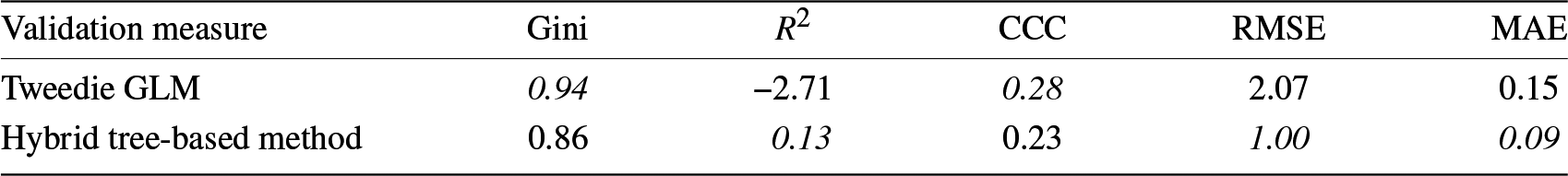
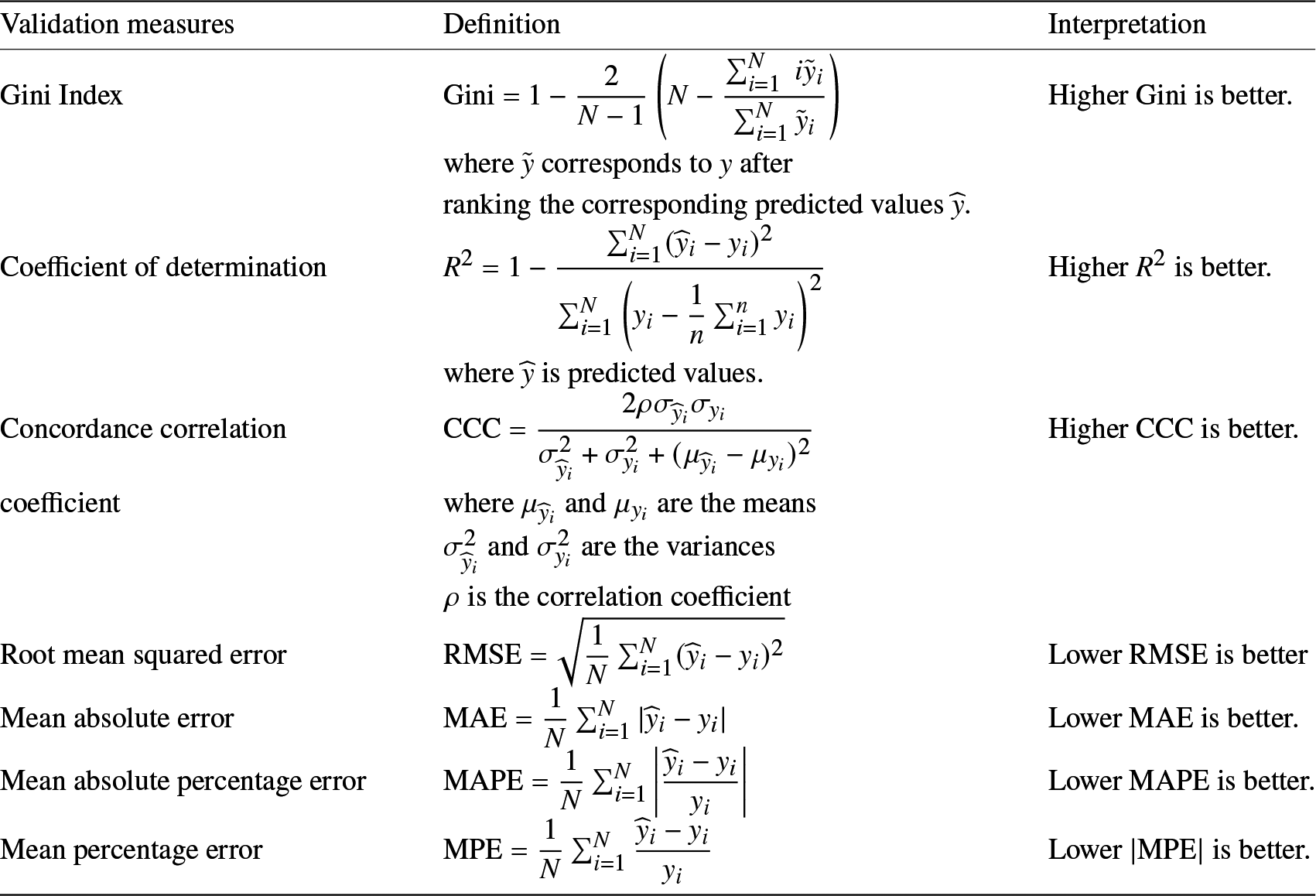
Once we have produced the simulated (or synthetic) dataset, we apply both the Tweedie GLM and hybrid tree-based methods to predict values of the response variables, given the available set of explanatory variables. The prediction performance between the two models is then compared using several validation measures as summarized in Table 1. In Appendix B, Table A1 describes details for validation measures. In many cases, machine learning models often outperform traditional statistical techniques regarding a single validation measure. This is especially true when machine learning models are optimized regarding that validation measure. To avoid choosing only the most beneficial results, we include more validation measures in the following study in order to draw a stronger and more comprehensive conclusion.

Table 1. Model performance on the simulation dataset.

CCC, concordance correlation coefficient.

From Table 1, we find that the Tweedie GLM’s fitting performance is worse even under the true model assumption, albeit in the presence of noise. As we described in Section 2, after hyperparameter tuning, hybrid tree-based methods with elastic net regression are able to automatically perform coefficient shrinkage via the L2 norm and variable selection based on the tree-structure algorithm and L1 norm. In a simulation setting that mimics real life, hybrid tree-based methods provide more promising prediction results than the widely accepted Tweedie GLM.

To rule out unfairness caused by improper variable selection, we reconstruct the simulation dataset without the nonrelevant explanatory variables. Therefore, the only difference from the previous simulated dataset is that we have 40 explanatory variables instead of 60. Using the same procedure, we obtain the model performance shown in Table 2. We can observe consistent results. Three out of five validation measures show that hybrid tree-based methods outperform the Tweedie GLM. However, the two weaker results are comparable.

Table 2. Model performance on the simulation dataset without nonrelevant explanatory variables.

CCC, concordance correlation coefficient.

In summary, we used a Poisson–gamma distribution within a two-part framework, adding some noise that mimics real-life situations to create the simulated datasets. Then, we compared the model accuracy between the Tweedie GLM and hybrid tree-based methods. We conclude that even under the linear assumption, hybrid tree-based methods can perform better than the Tweedie GLM.

4. Empirical application

We compare the Tweedie GLM with hybrid tree-based methods using one coverage group from the Wisconsin Local Government Property Insurance Fund (LGPIF) data. This dataset comes from a project at the University of Wisconsin’s actuarial research group, and further details about this dataset can be found on their website.Footnote ¹ The coverage group is called Building and Contents (BC), which provides insurance for buildings and properties of local government entities including counties, cities, towns, villages, school districts, and other miscellaneous entities. We draw observations from the years 2006 to 2010 as the training dataset and the year 2011 as the test dataset. Tables 3 and 4 summarize the training dataset and the test dataset, respectively.

Table 3. Summary statistics of the training dataset, 2006–2010.

Table 4. Summary statistics of the test dataset, 2011.

4.3. Model performance

We use several validation measures to examine the performance of different models, similar to what was done in the simulation. To make for an easier comparison, we added the heat map in addition to the prediction accuracy table based on various validation measures. We present results separately for training and test datasets. A rescaled value of 100 (colored blue) indicates that it is the best model among the comparisons; on the other hand, a rescaled value of 0 (colored red) indicates that it is the worst. For further details on this heat map for validation, see [Reference Quan and Valdez20].

From Figure 2(a), we find that the Tweedie GLM has the worst performance of model fit in general and the CART algorithm and HTGlm have better performance in model fitting. From Figure 2(b), we find that HTGlm has the best performance in the test dataset. It also shows that hybrid tree-based methods prevent overfitting compared to traditional regression trees using the CART algorithm. One possible reason is that the hybrid structure extrapolates the prediction range by using regression models at the terminal node. In general, hybrid tree-based methods perform consistently well for both training and test datasets. Because hybrid tree-based methods are considered piecewise linear models, the model generalization is inherited from the linear model. We can also note that HTGlmnet has a poorer performance compared to HTGlm, for both training and test datasets. The advantage of regularization does not demonstrate significant effects on the LGPIF dataset because of the limited number of explanatory variables. Furthermore, we observe a similar phenomenon as the CART algorithm also performs quite well compared to HTGlmnet, which is also likely a reflection of the fact that there are very few explanatory variables. However, in the simulation study, we showed the advantage of regularization because the data has a more significant number of explanatory variables. The simulated data may be a better replication of real-life insurance loss compared to LGPIF data with limited explanatory variables. It is also worth mentioning the discrepancy in the model performance regarding the Gini Index. Based on the definition of the Gini Index, the calculation involves ranking the predicted value. The Tweedie GLM and DNN predictions do not include a large number of zeros; however, in the hybrid structure, we assign zero prediction to a certain terminal node with a high percentage of zero claims. Consequently, the hybrid structure has an inferior performance regarding the Gini Index due to the uncertainty of ranking zero predictions. The DNN provides one aspect of the black-box model’s prediction performance. LGPIF dataset is not large enough for the DNN to observe the deep double descent phenomenon. In summary, hybrid tree-based methods outperform the Tweedie GLM based on various validation measures.

Figure 2. Heat maps of model comparison based on various validation measures. (a) Model performance based on training dataset. (b) Model performance based on test dataset.

5. Visualization and interpretation

The frequency component of hybrid tree-based methods can clearly be visualized as a tree structure like a simple CART algorithm. Here, we use HTGlm to illustrate the visualization and interpretation of hybrid tree-based methods. In Appendix C, Figure A1 shows the classification tree model for the frequency. We can follow the tree path and construct the density plot for the response variable for each node. This process will show a straightforward visualization of how the sample changes with every split. Figure 3 shows the classification tree, and we highlighted (blue) nodes two depths away from the root. Consequently, we have seven nodes including the root nodes. Here we denote the node with numbers for the purpose of identification. Among the highlighted nodes, node four (4), on the left, is the terminal node and the others are intermediate nodes. Figure 4 shows the density of the response variable for the seven nodes mentioned in Figure 3. For better visualization, Figure 4 presents the logarithm of one plus the claim amounts instead of the actual claim amounts. The root node has zero point mass, as expected, and the black dashed line is the mean of the response variable at the node. After the first split using CoverageBC, the mean shifted toward a different direction, and the percentage of the point mass at zero also changed in a different direction. At the fourth terminal node, we can barely see any positive claims with the mean shifting toward zero, and this terminal node ultimately assigns zero as the prediction. We can see that the classification tree algorithm, done by recursive binary splitting, divides the dataset into subspaces that contain more similar observations. The same phenomenon can also be observed in the CART algorithm, which uses a tree structure to separate similar data to the same group in the terminal node and then uses mean or mode as the predicted value. For the same reason, the proposed simple hybrid tree-based method applies linear models with the Gaussian family in the terminal node without setting the choice of distribution as a tuning parameter. After dividing the space of explanatory variables into subspaces, it may be more appropriate to make distribution assumptions and apply the linear model to the subsamples. In a sense, hybrid tree-based methods employ a “divide and conquer” algorithm, which may be a promising solution for imbalanced datasets.

Figure 3. Tree paths with highlighted nodes.

Figure 4. Classification tree for the frequency.

Figure 5. Variable importance for the claim frequency.

Figure 3 shows the path to terminal nodes, and we can see a zero or a one, where a linear model is then fitted, for each terminal node. The structure and path of the tree can provide an indication of the risk factors based on the split of the explanatory variables. Figure 5 shows the variable importance calculated from the classification tree model for the frequency part. Coverage and deductible information are much more important than location and previous claim history to identify whether the claim occurred or not. It is not surprising that the deductible has an important impact on claim frequency, as a claim occurrence will occur only if the amount exceeds the deductible. At each terminal node, we can also extract the regression coefficients and interpret the estimated linear regression model. Table 5 provides the regression coefficients at each of the nonzero terminal nodes. The node number has the same label as in Figure 3. For example, the terminal node 245 can be reached as follows: $CoverageBC\geq2$, TypeCounty, $Coverage\geq3.5$, $lnDeductBC\geq7.4$, $CoverageBC\geq3.8$, lnDeductBC < 10, and lnDeductBC < 9.9, and we estimated the linear model with regression coefficients: $Intercept=-172,854$, $CoverageBC=15,251$, $lnDeductBC=16,777$, and $NoClaimCreditBC=-16,254$. Similarly, Eq. (1) can be specified based on the tree structure and regression coefficients. Hence, we are able to write out the hybrid tree-based method in the piecewise linear form.

At the terminal node, the linear model is built that is based on the regularized algorithm and is based solely on the accuracy of the prediction from cross-validation. It does not rely on statistical inference, and indeed, some regression coefficients are not statistically significant. However, we can tune hybrid tree-based methods by balancing prediction accuracy and statistical inference. For example, when we try to measure the impact of a specific explanatory variable on the claim severity, the coefficient should be statistically significant. To find the reliable coefficient, we might attempt to merge some child nodes or split the dataset further and then build another regression model. It is possible that these attempts may not yield optimal prediction performance due to the fact that statistical inference is prioritized over prediction accuracy.

Table 5. Regression coefficients at the terminal nodes.

The primary advantage of hybrid tree-based methods is its intuitive interpretability. It is possible to extend our approach that considers ensemble techniques such as boosting or bagging using hybrid tree-based methods as base learners. Such extensions can significantly improve prediction accuracy, however, sacrificing model interpretability.

Furthermore, hybrid tree-based methods may capture the dependence between frequency and severity. Based on the hybrid structure, the severity model is conditionally built on tree-based partitions created using frequency information. Hence, it inherently allows for a certain dependence between frequency and severity. We observe this phenomenon in Table 5. Most regression coefficients at the terminal nodes do not include location information, which might already be incorporated into the tree-based model. With this in mind, the proposed hybrid tree-based method has an added advantage over the traditional Tweedie GLM, which assumes that frequency and severity are independent under the compound Poisson–gamma framework.