


Introduction
Micro computed tomography, or micro-CT, has rapidly evolved as a leading technique for 3D non-destructive microstructural characterization. Simply put, micro-CT collects a series of images around a sample, using x-rays as the signal. Those images are then combined into a virtual 3D reconstruction of the original sample that includes internal details. X-rays, as opposed to electrons or visible light used in surface characterization techniques, penetrate and interact with a wide range of materials, providing useful information about the internal features without the need to physically section the sample. While 2D x-ray imaging has been widely used for over 120 years, 3D techniques emerged in medical applications about 60 years ago with higher resolution 3D imaging (that is, micro-CT) making its appearance in the early 1980s. The first micro-CT systems obtained resolutions on the order of 50–100 μm. Since then, and especially in the last 20 years, the resolution has improved tremendously with some nano-CT systems reaching a resolution below 100 nm. Sub-micron (500–1000 nm) systems are becoming commonplace in academia and industrial research departments to better understand material fundamentals, while “industrial” CT systems with resolution ranging from a few micrometers to millimeters are more prevalent in production settings.
With micro-CT being recognized as an essential technique and with wide commercial availability, it is natural for scientists and engineers to push the boundaries of 3D x-ray imaging. In situ imaging, where samples are subjected to some type of stimulus, is one clear example. Synchrotron facilities, where the available flux of x-ray photons can be a billion times higher than what is possible in the lab, have been at the forefront of imaging advancements. To this point, over the last 10+ years there has been substantial emphasis on imaging evolving structures, typically via in situ testing. Whether it's loading of materials [Reference Cheng and Wang1–Reference Butler2], heating of samples [Reference Saif3], fluid flow inside a sample [Reference Bultreys4], or examining the beat of an insect's wing [Reference Walker5], speed of data collection is critical. With some synchrotrons it is possible to collect hundreds of full tomography datasets per second, which is crucial for data collection in processes that involve rapid changes in metallic foams [Reference García-Moreno6]. In the lab in situ work is certainly possible, however, it has typically been limited to slow processes (hours to days) or interrupted testing (for example, compressive testing where loading is performed step-wise and imaging is done while there is no change in loading) [Reference Patterson7]. To bridge the gap between the synchrotron and the lab, TESCAN has developed a series of hardware and software tools that make scan speeds on the order of seconds possible and enable dynamic CT capability in a laboratory setting [Reference Dewanckele8]. There are some limitations related to sample size, resolution, and image noise, but these are practical issues that will be overcome as the technology moves forward.
The aim of this paper is to highlight recent examples where the temporal resolution of CT imaging is pushed. We will demonstrate how dynamic CT in the lab can contribute to better understanding of processes in geosciences and material sciences.
Basics of Micro-CT
With computed tomography, a tomogram is created by the relative rotation of a sample between an x-ray source and detector while collecting a series of 2D radiographs at different angular locations and then reconstructing the data into a full 3D data set. In some cases, the sample is stopped at each step, called step-and-shoot, whereas in other cases the sample continuously rotates, for example, continuous, or smooth CT. The 2D radiographs are essentially grayscale images of the sample where the gray level at each pixel location corresponds to the overall x-ray attenuation of the material along that path. Once the radiographs are collected, they are processed through a reconstruction algorithm resulting in a stack of 2D slices, which make up a full 3D volume of the original sample [Reference Feldkamp9]. The basic system design and workflow are illustrated in Figure 1. The resultant 3D data set provides insight about the internal features of the sample as well as relative density differences. The primary influences on the quality of the data are the resolution of the system and the type and size of sample. The spatial resolution of a system (R sys) is predominantly a function of the x-ray source spot (R source), the detector resolution (or pixel size) (R dect), and the geometric relation of the sample (Geo Mag), source, and detector (equation 1):
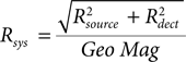
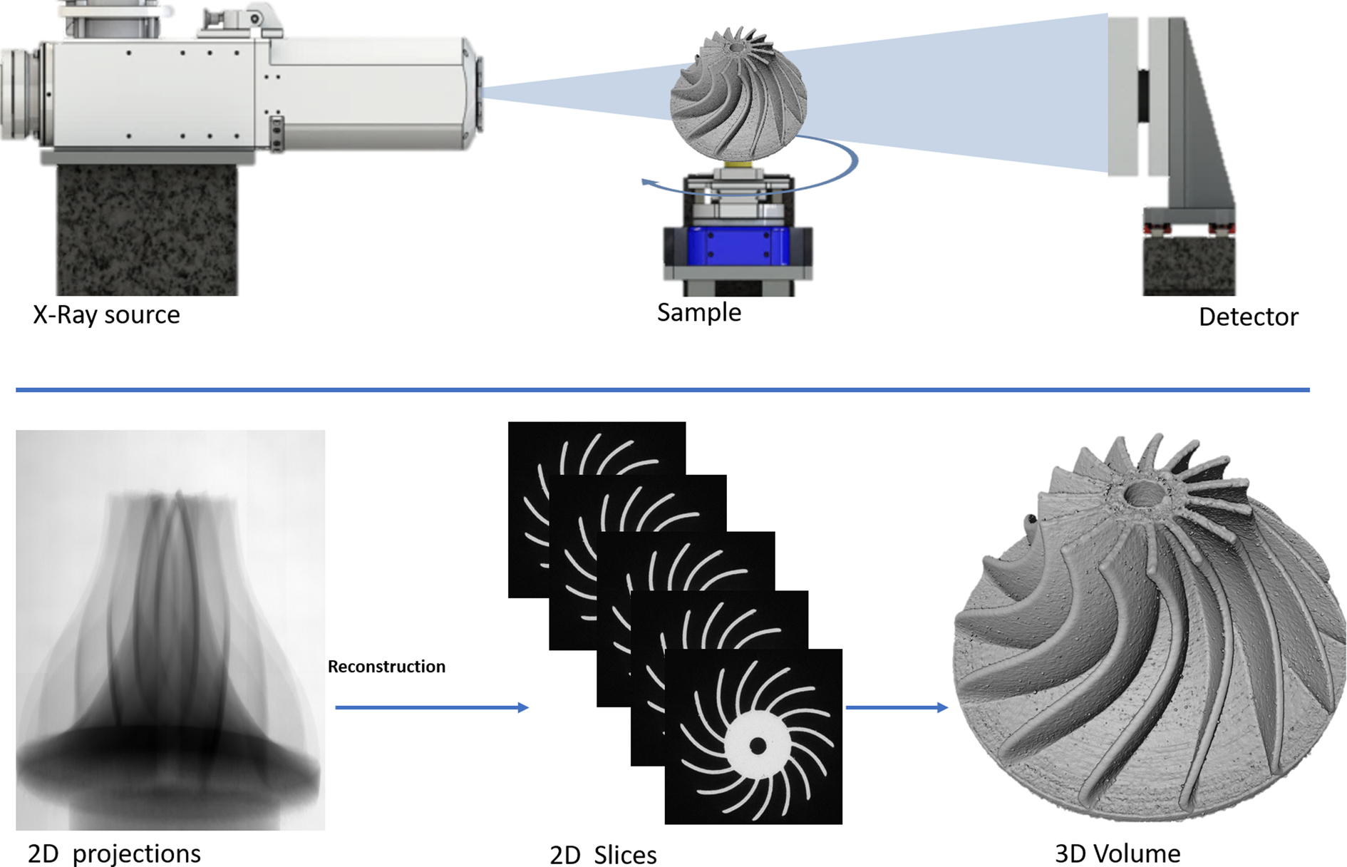
Figure 1: Top: basic schematic of typical micro-CT system with an x-ray source (left), rotating sample (center), and detector (right). Bottom: 2D projections (left) are collected at multiple angles and processed by a reconstruction algorithm to produce 2D slices through the sample (center), which can then be visualized and analyzed in 3D (right).
Although voxel size is often used in place of spatial resolution, it is important to note that voxel size is only a function of the geometric relation of the components and the detector pixel size, while for true spatial resolution the size of the x-ray spot must be taken into account. The ability of x-rays to penetrate and interact with the sample is the other primary influence on image quality.
For a given x-ray energy, the attenuation of photons will vary dramatically as the atomic weight of the sample material increases. This creates a limit on thickness (size) of a sample depending on the type of material, or a requirement to use higher x-ray energy, often at the cost of a larger spot size and thus decreased resolution. For the most part micro-CT, where spatial resolutions below 10 μm are possible, will use energies below ~240 kV. Additionally, mixed material systems, especially ones with a wide variance in atomic weight (that is, metal wires in a rubber matrix), may create imaging artifacts due to the vastly different x-ray attenuations of the materials relative to one another. Several examples of static (non-dynamic) CT data are shown in Figure 2.
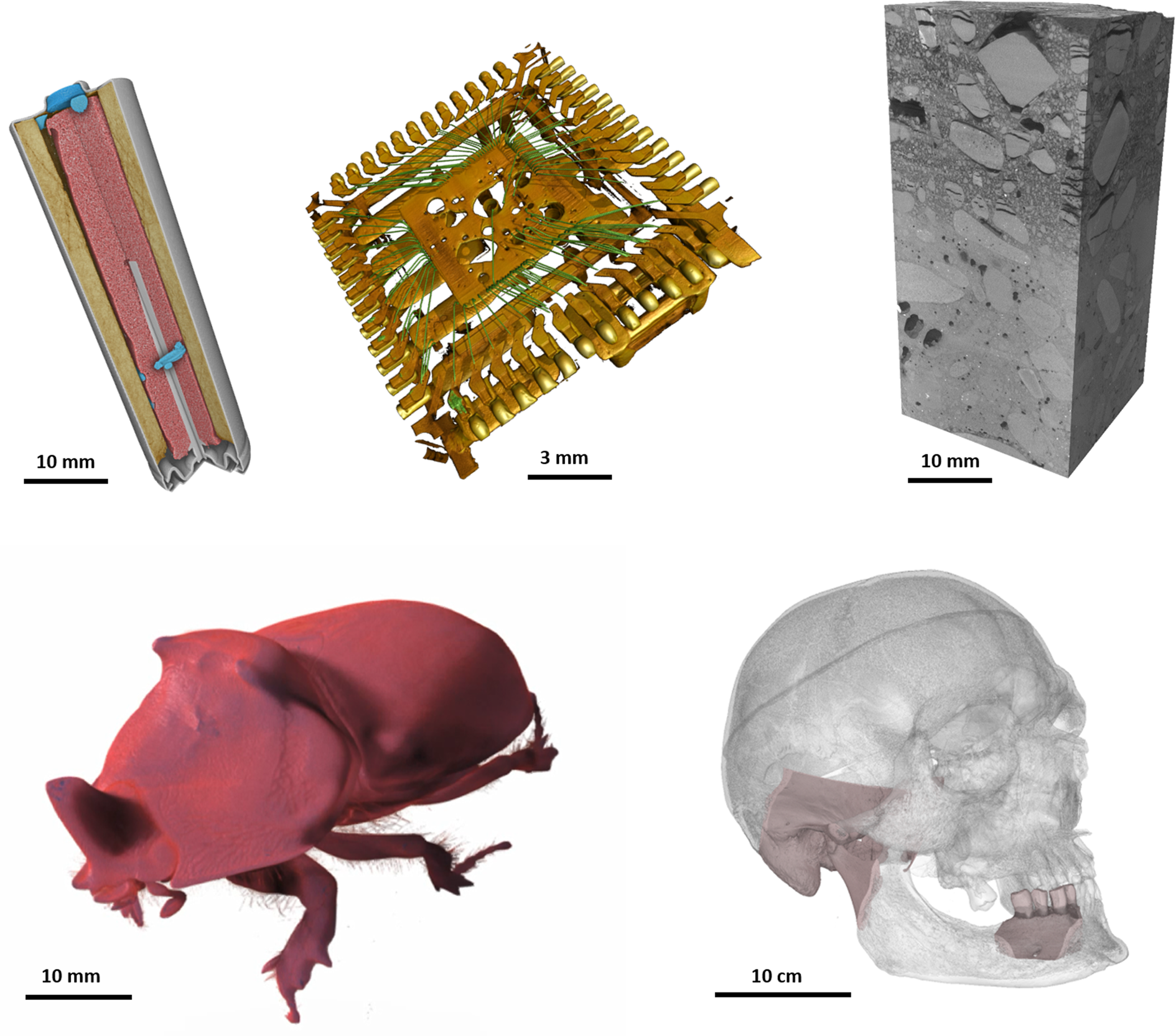
Figure 2: Examples of CT data. (Clockwise from top left) Segmented AA alkaline battery, metal in an integrated circuit (IC) package, weathered concrete, Rhinoceros beetle, and an entire human skull. Scale bars for reference only.
From 3D to 4D: Adding the Temporal Component
In general, the greatest advantage of micro-CT worth comes from its non-destructive nature. The ability to investigate internal structures of a sample without cutting it open has been extremely beneficial in several areas, for instance, failure analysis and quality control in common industrial applications [Reference du Plessis10]. The continued development of correlative workflows, where CT data are used to better educate an investigator on where to examine a part at higher resolution through physical cross section techniques, that is, FIB-SEM, has also become a very valuable tool in materials and life science characterization [Reference Song11]. However, one of the most exciting uses for micro-CT over the last several years has been to leverage the non-destructive nature to investigate temporal events, allowing one to track the 3D evolution of a structure as it undergoes some type of change. Whether through applying an external load, that is, compression/tension, inducing a change in material through thermal effects, or mixing and interaction of fluids in a porous network, the ability to understand these changes in 3D will be a great boon to scientists and researchers across many fields.
Dynamic versus Time-Lapse
In situ experimentation with micro-CT has led to a great number of new insights into how things change when subjected to different stimuli. However, in most cases, the experiments have been limited to processes that occur slowly, or there is a requirement to interrupt the process at certain time points to collect data. This is referred to as time-lapse tomography, where data are collected at certain time points, but there is discontinuity in the data as no information about what is happening between these discrete points is available. For dynamic CT, a continuous acquisition method is used where imaging is never stopped throughout the process. This provides a much more complete picture of the sample evolution and allows for much more flexibility in terms of working with the collected data. Continuous acquisition eliminates the reliance on fixed individual 360o rotations of data; it is possible to shift reconstruction blocks and, in some cases, overlap reconstruction blocks to provide the most useful information possible in a process called “sliding window reconstruction” [Reference Dewanckele8,Reference Bultreys12]. Additionally, many time-dependent processes are unpredictable, and capturing the most important aspects of the process may not be possible in an interrupted or time-lapse collection scheme. With dynamic CT, this issue is resolved by collecting data throughout the entire process, providing a wealth of information previously unavailable to researchers. To better illustrate the concept of dynamic CT, several case studies are presented.
Dynamic CT Case Studies
Uninterrupted compression testing: additive manufacturing (AM).
3D printing is a quickly emerging production process for many applications in medicine and the aerospace industry. As with many manufactured parts, AM products can be prone to both external and internal defects. These defects, such as voids, cracks, delamination, and contaminants, may influence the mechanical performance of a product. However, the complex geometry possible with AM creates unique challenges for inspection. Micro-CT, which provides non-destructive 3D information about a part, has become essential for detection and analysis of internal imperfections in these intricate parts [Reference Thompson13]. Aside from basic quality analysis, it is also essential to understand how these imperfections influence the behavior of the part when they are actually used. Dynamic CT can provide detailed information on a part's actual performance.
As mentioned previously, most lab-based in situ micro-CT involving loading a part in compression or tension is done in an interrupted form, where the applied force must be held constant during the tomography collection. This sometimes creates issues involving sample relaxation and missing information during the actual loading procedure [Reference Carlton14]. Dynamic CT, with continuous acquisition and uninterrupted loading, helps to alleviate these issues. As an example, several different test specimens were created in plastic using 3D printing. A total of six cylindrical samples, with different internal supports, were formed. Each sample was then compressed continuously using a Deben load stage, while tomography data were collected on a TESCAN CoreTOM at a rate of one sample rotation every 5.8 seconds with a voxel resolution of 59 µm. This resulted in 210 full sample scans for each sample. Figure 3 provides an overview of three of these samples including their internal structure, 3D rendered snapshots of the sample throughout the process, and their associated load curves. Through this experimental evaluation of deformation of different geometries, one can develop more precise simulations to best understand optimization for the specific needs of an application. As can be seen on the graph, no relaxation took place during the experiment due to a constant displacement.

Figure 3: Example of 3 different plastic additive manufactured (AM) parts that have undergone compression testing while being continuously imaged with dynamic CT. Only 4 images out of 210 collected are shown here.
Imaging of beer foam.
Everyone loves a good beer, but what makes a beer good? One could certainly argue that the foam plays an important role, but why? In this experiment, we examine the collapse of a beer foam and compare the differences between two different types of beer. In one case the foam stays intact over a long period of time while the foam dissipates quite quickly in the second case. Why is this important? Smell is an integral part of taste, and the beer head acts as a carrier for the aromatics of a beer. The fact that a beer that goes “flat” tastes different isn't just because there is less “fizziness,” but it's also because the aromatics are less available, therefore changing the taste of the beer. In this experiment [Reference Dewanckele8] the authors imaged two different beer types in the TESCAN DynaTOM, a unique gantry-based system where the sample remains stationary while the x-ray source and detector rotate. This allows for a maximum amount of flexibility when working with complex in situ samples or, as is the case with beer foam, delicate samples that may be distorted by the simple action of rotating the sample in a traditional micro-CT system. For beer 1, a Belgian strong ale, 70 rotations about the sample with 15 seconds per full 360o rotation at 160 µm voxel size were collected, resulting in a total experiment time of 17.5 minutes. For beer 2, a lager, the conditions were slightly different with 80 rotations about the sample, 9.4 seconds per full 360o rotation, and 150 µm voxel size, resulting in a total experiment time of 12.5 minutes. The foam from each sample was then analyzed to show the relation of the average equivalent diameter (AED) of the pores and the height of the foam, resulting in some stark differences between the two beverages. In the Belgian ale, a much smaller equivalent pore diameter, resulting in a much more resilient and dense foam, was observed in comparison with the lager. A main takeaway of this experiment: make sure to drink a lager beer quickly, but take some time when enjoying an expressive and flavorful Belgian strong ale! In all seriousness, this type of imaging and analysis can be transferred to several other lightweight foam applications, including the evolution of polymeric foams during production or under corrosive environments. Figure 4 provides a comparison of 3D renderings of the foam of the two different beers at several time points, while Figure 5 demonstrates segmented results of the foam pores at different time points for the Belgian strong ale.

Figure 4: 3D renderings of three different time points (0, 2, and 9 minutes) of the beers used for this comparison. Clear differences are seen in the consistency of the foam head between the two types of beer. The lager foam has all but disappeared by 9 minutes, while the strong ale is holding up well. Modified from [Reference Dewanckele8].

Figure 5: Segmentation and analysis of the foam pore sizes was performed across all 80 data sets. Shown are examples at 4 different time points, where the color represents the size of the pore (blue, smallest; red, largest). Modified from [Reference Dewanckele8].
In situ two-phase flow in porous media.
Two-phase flow in porous media has been studied extensively in several areas such as oil and gas, environmental sciences, and alternative energy [Reference Held15]. Although lab-based micro-CT has been performed to study this interaction [Reference Prodanović16], the information gathered has almost always been with the sample in an equilibrium state. Typically, the sample is imaged with one phase, a second phase is introduced and allowed to come to steady state, and then the sample is imaged again with both phases present. This provides a nice snapshot of the before and after but provides little information concerning the ongoing state as the second phase is introduced. With the advent of lab-based dynamic micro-CT acquisition, researchers are now able to explore these interim states. As an example, a sintered glass sample was saturated with a brine solution (containing 2 wt % CsCl as the contrast agent) followed by introduction of an oil phase (n-decane). Both the sample and filter were placed in a Viton sleeve, and a confining pressure was applied around the sleeve. To achieve full water saturation, the sample was first flushed with CO2 at 2 bars for 5 minutes from the top, followed by water pumped from the bottom (20 μL/min for 1 hour) until it was through the sample. Next, brine was continuously pumped through the sample until the CO2 was removed from the pore space. Finally, the oil was introduced from the top by changing the direction of the pump (bottom of flow cell).
The primary goal for this test was to better understand the drainage behavior in geological porous materials when undergoing uninterrupted oil injection. Tomographic data were continuously collected in the TESCAN DynaTOM, a unique gantry-based instrument that allows for complex in situ setups, which are not suitable with traditional micro-CT architectures where the sample is required to rotate. A total of 80 scans were collected over a period of 10 minutes, with each rotation of the sample taking 7.5 seconds at 12.5 μm voxel size. Figure 6 shows a picture of the sample setup in the system, while Figure 7 shows several 3D renderings at different time points. The red areas indicate location of oil infiltration through the porous network. After a time, the flow was paused and the micro-CT system was reconfigured for higher resolution, in this case 4.5 μm voxel size, with each rotation taking 60 seconds. Figure 8 provides some detail of the higher resolution imaging in the form of virtual cross sections through the sample at different time points. The lightest phase is the fused silica, the intermediate phase is the brine, and the darkest phase is the oil. Although a bit slower, clear infiltration of the oil into the brine-saturated network can be seen.
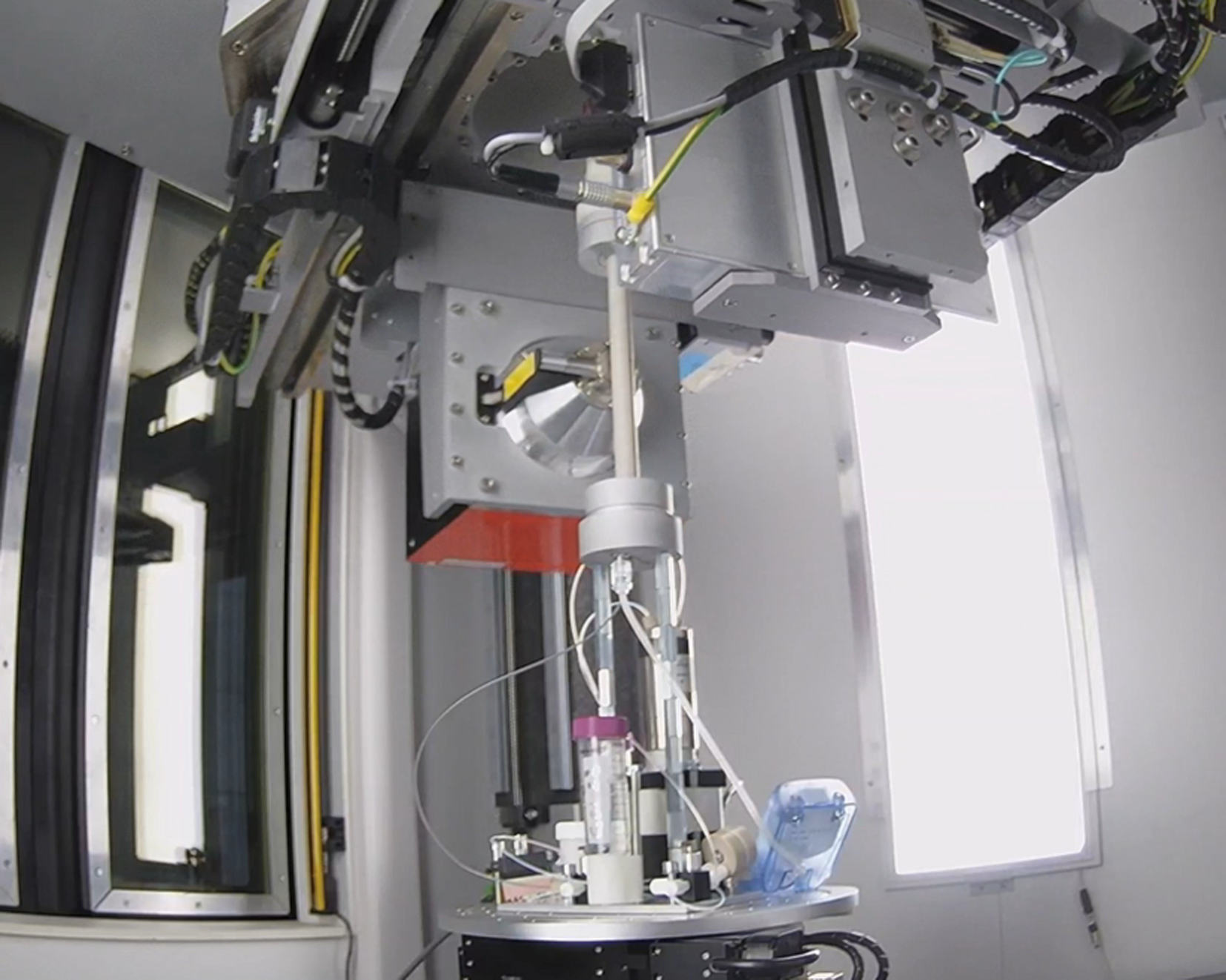
Figure 6: Flow cell mounted in DynaTOM. The unique horizontally rotating gantry of the system allows for complex in situ dynamic CT such as complex flow experiments.
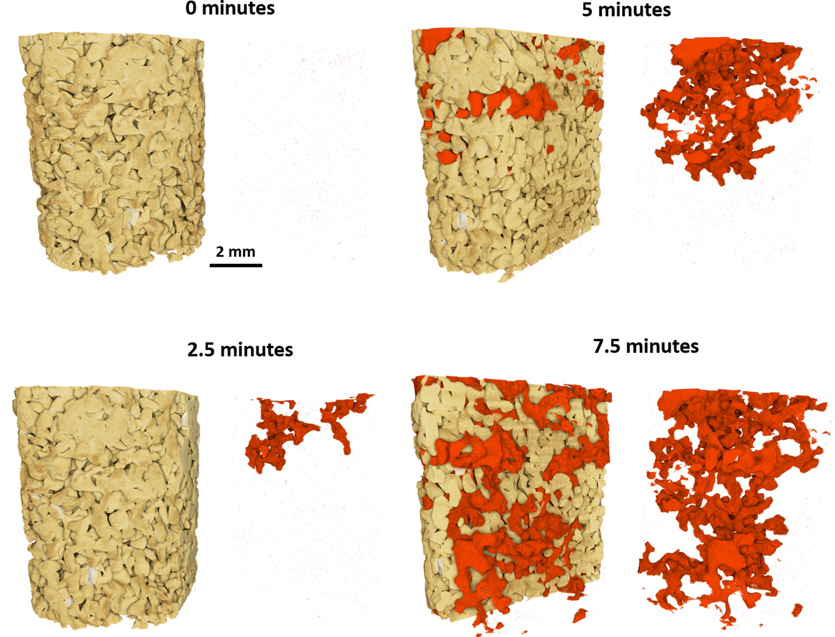
Figure 7: 3D rendered images showing the full sample at four different time points during a dynamic experiment, without interrupting the injection of oil (red) (0, 2.5, 5, and 7.5 minutes).
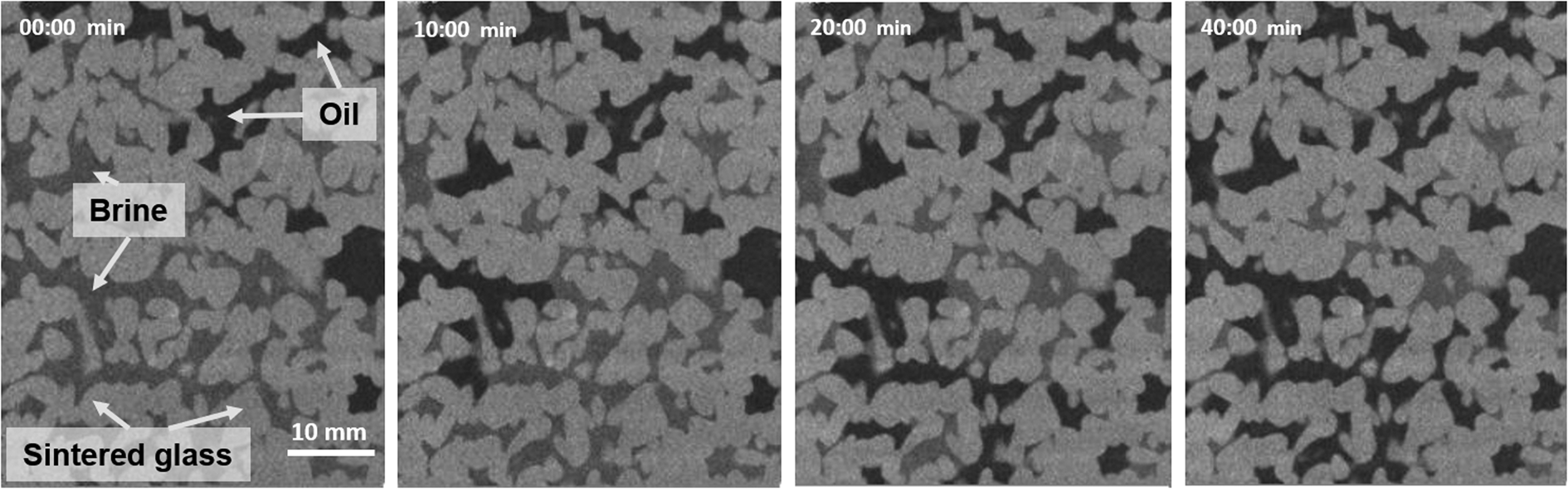
Figure 8: Virtual cross sections at 4 different time points (0, 10, 20, 40 minutes) for the volume of interest (VOI) scan. All three phases are clearly distinguishable at 4.5 μm voxel resolution and 60 seconds per rotation.
Summary
Micro-CT has become a more commonplace technique over the past decade, providing invaluable non-destructive 3D information for a variety of research and industrial applications. With the advent of higher-powered sources and faster detectors, coupled with specialized software and application experience, lab-based micro-CT is now pushing into a new realm of temporal resolution, allowing for true dynamic CT experiments. The future of micro-CT is vast and virtually unlimited, and it's certainly an exciting time to be a part of these developments. The possibility to scan and analyze fast dynamic experiments opens doors for many other more in-depth studies.


