


1. Introduction
This paper contributes to the literature on empirical macroeconomic models with time-varying conditional moments, by introducing the heteroskedastic score-driven state-space model with Student’s $t$
-distributed innovations, in which both location and scale are score-driven, and illustrating the model performance in an empirical macroeconomic model applied to a well-known dynamic stochastic general equilibrium (DSGE) model [Kydland and Prescott (Reference Kydland and Prescott1982), Long and Plosser (Reference Long and Plosser1983)].
$t$
-distributed innovations, in which both location and scale are score-driven, and illustrating the model performance in an empirical macroeconomic model applied to a well-known dynamic stochastic general equilibrium (DSGE) model [Kydland and Prescott (Reference Kydland and Prescott1982), Long and Plosser (Reference Long and Plosser1983)].
From a methodological perspective, this paper contributes to the well-developed literature on modeling time variation in multivariate econometric models. In the works of Canova (Reference Canova1993), Sims (Reference Sims and Sims1993), Stock and Watson (Reference Stock and Watson1996), and Cogley and Sargent (Reference Cogley and Sargent2001), vector autoregressive (VAR) models with drifting coefficients and homoskedastic errors are used. By using multivariate stochastic volatility models [Harvey, et al. (Reference Harvey, Ruiz and Shephard1994)] for the innovations, the works of Cogley and Sargent (Reference Cogley and Sargent2005) and Primiceri (Reference Primiceri2005) present VAR models with drifting coefficients and stochastic volatility. In the work of Chan and Eisenstat (Reference Chan and Eisenstat2018), the performances of VAR models with drifting coefficients and stochastic volatilities, and VAR models with time-invariant coefficients and stochastic volatilities are compared. Those authors find that, given conditional heteroskedasticity, there is no need for drifting coefficients in the VAR model. The empirical macroeconomic model of our paper fits into that literature. In the heteroskedastic score-driven state-space model with Student’s $t$
-distributed innovations [also named heteroskedastic
$t$
-distributed innovations [also named heteroskedastic $t$
-QVAR, quasi-VAR, model], the coefficients are time-invariant and the error terms are conditionally heteroskedastic, similar to the best-performing model of Chan and Eisenstat (Reference Chan and Eisenstat2018). The
$t$
-QVAR, quasi-VAR, model], the coefficients are time-invariant and the error terms are conditionally heteroskedastic, similar to the best-performing model of Chan and Eisenstat (Reference Chan and Eisenstat2018). The $t$
-QVAR model is a nonlinear extension of the VARMA (VAR moving average) model.
$t$
-QVAR model is a nonlinear extension of the VARMA (VAR moving average) model.
Score-driven models [Creal et al. (Reference Creal, Koopman and Lucas2008, Reference Creal, Koopman and Lucas2011, Reference Creal, Koopman and Lucas2013); Harvey and Chakravarty (Reference Harvey and Chakravarty2008), Harvey (Reference Harvey2013)] are observation-driven models [Cox (Reference Cox1981)], in which the filters are updated by the scaled partial derivatives of the log-likelihood (LL) of the dependent variables with respect to dynamic parameters (i.e., scaled score functions). The following statistical advantages of score-driven time series models motivate their use in our paper: (i) score-driven models are robust to outliers and missing data [Harvey (Reference Harvey2013), Blazsek and Escribano (Reference Blazsek and Escribano2016, Reference Blazsek and Escribano2022), Ayala et al. (Reference Ayala, Blazsek and Escribano2022)]. (ii) Score-driven models are generalizations of observation-driven time series models [e.g., ARMA model; generalized AR conditional heteroskedasticity model; VARMA model] [see in the work of Harvey (Reference Harvey2013)]. (iii) In the work of Blasques et al. (Reference Blasques, Koopman and Lucas2015) it is shown for score-driven models that a score-driven update locally reduces the Kullback–Leibler divergence in expectation at every step asymptotically.
We use the heteroskedastic $t$
-QVAR model to estimate a heteroskedastic score-driven
$t$
-QVAR model to estimate a heteroskedastic score-driven $t$
-ABCD representation of the DSGE model of An and Schorfheide (Reference An and Schorfheide2007). The
$t$
-ABCD representation of the DSGE model of An and Schorfheide (Reference An and Schorfheide2007). The $t$
-ABCD representation is an extension of the Gaussian-ABCD representation [Fernández-Villaverde et al. (Reference Fernández-Villaverde, Rubio-Ramírez, Sargent and Watson2007)] and the heteroskedastic score-driven Gaussian-ABCD representation [Angelini and Gorgi (Reference Angelini and Gorgi2018)]. We report results by using data on economic output, inflation, interest rate, government spending, aggregate productivity, and consumption of the USA for the period of 1954 Q3 to 2022 Q1. We find a superior statistical performance, lower policy-relevant dynamic effects, and a higher estimation precision of the impulse response function (IRF) for US gross domestic product (GDP) growth and US inflation rate, for the heteroskedastic score-driven
$t$
-ABCD representation is an extension of the Gaussian-ABCD representation [Fernández-Villaverde et al. (Reference Fernández-Villaverde, Rubio-Ramírez, Sargent and Watson2007)] and the heteroskedastic score-driven Gaussian-ABCD representation [Angelini and Gorgi (Reference Angelini and Gorgi2018)]. We report results by using data on economic output, inflation, interest rate, government spending, aggregate productivity, and consumption of the USA for the period of 1954 Q3 to 2022 Q1. We find a superior statistical performance, lower policy-relevant dynamic effects, and a higher estimation precision of the impulse response function (IRF) for US gross domestic product (GDP) growth and US inflation rate, for the heteroskedastic score-driven $t$
-ABCD representation rather than for the homoskedastic Gaussian-ABCD representation. This is due to the robustness of the heteroskedastic
$t$
-ABCD representation rather than for the homoskedastic Gaussian-ABCD representation. This is due to the robustness of the heteroskedastic $t$
-QVAR model.
$t$
-QVAR model.
The remainder of this paper is organized as follows: Section 2 presents the econometric model. Section 3 presents the empirical application. Section 4 concludes.
2. Score-driven empirical macroeconomic models with heteroskedastic innovations
2.1. A Gaussian linear state-space model
For the purpose of explanation, we start with a Gaussian linear state-space model, which is extended to the heteroskedastic $t$
-QVAR model in this paper. The observable variables are collected into the vector
$t$
-QVAR model in this paper. The observable variables are collected into the vector $Y_{t}$ $(\mathcal{N}\times 1)$
and the state variables are collected into the vector
$(\mathcal{N}\times 1)$
and the state variables are collected into the vector $X_{t}$ $(\mathcal{N}\times 1)$
. The first representation of the Gaussian linear state-space model is the following system of equations:
$(\mathcal{N}\times 1)$
. The first representation of the Gaussian linear state-space model is the following system of equations:
 \begin{equation} X_{t}=A X_{t-1}+B \epsilon _{t} \end{equation}
 \begin{equation} Y_{t}=C X_{t-1}+D \epsilon _{t} \end{equation}
where $\epsilon _{t}$ $(\mathcal{N}\times 1)$
has an i.i.d. multivariate normal distribution
$(\mathcal{N}\times 1)$
has an i.i.d. multivariate normal distribution $\epsilon _{t}\sim N(0,\Omega \Omega^{\prime})$
and a diagonal covariance matrix
$\epsilon _{t}\sim N(0,\Omega \Omega^{\prime})$
and a diagonal covariance matrix $\Omega \Omega^{\prime}$
. The parameter matrices are
$\Omega \Omega^{\prime}$
. The parameter matrices are $A$
,
$A$
, $B$
,
$B$
, $C$
, and
$C$
, and $D$
, which are square matrices with dimensions
$D$
, which are square matrices with dimensions $(\mathcal{N} \times \mathcal{N})$
. If matrix
$(\mathcal{N} \times \mathcal{N})$
. If matrix $D$
is non-singular, then, by using the reduced-form error
$D$
is non-singular, then, by using the reduced-form error $v_{t}\equiv D \epsilon _{t}$
, an equivalent representation of the system of Equations (1) and (2) is
$v_{t}\equiv D \epsilon _{t}$
, an equivalent representation of the system of Equations (1) and (2) is
 \begin{equation} X_{t}=A X_{t-1}+B D^{-1} v_{t} \end{equation}
 \begin{equation} Y_{t}=C X_{t-1}+v_{t} \end{equation}
where $v_{t}\sim N(0,\Sigma )\equiv N[0,D\Omega \Omega^{\prime}D^{\prime}]$
is the multivariate i.i.d. reduced-form error term. Moreover, if
$v_{t}\sim N(0,\Sigma )\equiv N[0,D\Omega \Omega^{\prime}D^{\prime}]$
is the multivariate i.i.d. reduced-form error term. Moreover, if $C$
is non-singular, then we get the following Gaussian-VARMA(1,1) representation:
$C$
is non-singular, then we get the following Gaussian-VARMA(1,1) representation:
 \begin{equation} Y_{t}=C A C^{-1} Y_{t-1} + \left(C B D^{-1} -C A C^{-1}\right)v_{t-1}+v_{t} \end{equation}
The reduced-form representation of Equations (3) and (4) is extended to the heteroskedastic $t$
-QVAR model according to the following points. In the heteroskedastic
$t$
-QVAR model according to the following points. In the heteroskedastic $t$
-QVAR model, (i)
$t$
-QVAR model, (i) $v_{t}$
has a multivariate
$v_{t}$
has a multivariate $t$
-distribution with degrees of freedom
$t$
-distribution with degrees of freedom $\nu$
, (ii)
$\nu$
, (ii) $v_{t}$
is conditionally heteroskedastic, and (iii) the updating term
$v_{t}$
is conditionally heteroskedastic, and (iii) the updating term $v_{t}$
in Equation (3) is replaced by the score function
$v_{t}$
in Equation (3) is replaced by the score function $u_{t}$
, for which we have that
$u_{t}$
, for which we have that $u_{t} \rightarrow _{p} v_{t}$
if
$u_{t} \rightarrow _{p} v_{t}$
if $\nu \rightarrow \infty$
. The resulting heteroskedastic
$\nu \rightarrow \infty$
. The resulting heteroskedastic $t$
-QVAR model is presented in the following section.
$t$
-QVAR model is presented in the following section.
2.2. Heteroskedastic score-driven $t$
-QVAR model
$t$
-QVAR model

The first representation of the heteroskedastic $t$
-QVAR model is
$t$
-QVAR model is
 \begin{equation} X_{t}=A X_{t-1}+B D^{-1} u_{t} \end{equation}
 \begin{equation} Y_{t}=C X_{t-1}+D \epsilon _{t} \end{equation}
where $D$
is non-singular and
$D$
is non-singular and $\epsilon _{t}|\mathcal{F}_{t-1}\sim t(0,\Omega _{t}\Omega^{\prime}_{t},\nu )$
is a multivariate
$\epsilon _{t}|\mathcal{F}_{t-1}\sim t(0,\Omega _{t}\Omega^{\prime}_{t},\nu )$
is a multivariate $t$
-distribution with scale matrix
$t$
-distribution with scale matrix $\Omega _{t}\Omega^{\prime}_{t}$
and degrees of freedom
$\Omega _{t}\Omega^{\prime}_{t}$
and degrees of freedom $\nu \gt 2$
, where the sigma algebra is
$\nu \gt 2$
, where the sigma algebra is $\mathcal{F}_{t-1}=\sigma (Y_{1},\ldots,Y_{t-1},X_{1},\Omega _{1})$
. We use parameter vector
$\mathcal{F}_{t-1}=\sigma (Y_{1},\ldots,Y_{t-1},X_{1},\Omega _{1})$
. We use parameter vector $X_{0}$
, which is jointly estimated with the rest of the time-invariant parameters, to initialize the state variables
$X_{0}$
, which is jointly estimated with the rest of the time-invariant parameters, to initialize the state variables $X_{t}$
. Technical details for the updating term
$X_{t}$
. Technical details for the updating term $u_{t}$
(i.e., scaled score function) are presented in Section 2.3. By using the reduced-form error
$u_{t}$
(i.e., scaled score function) are presented in Section 2.3. By using the reduced-form error $v_{t}\equiv D \epsilon _{t}$
, the second representation is
$v_{t}\equiv D \epsilon _{t}$
, the second representation is
 \begin{equation} X_{t}=A X_{t-1}+B D^{-1} u_{t} \end{equation}
 \begin{equation} Y_{t}=C X_{t-1}+v_{t} \end{equation}
where $v_{t}|\mathcal{F}_{t-1}\sim t(0,\Sigma _{t},\nu )\equiv t(0,D \Omega _{t}\Omega^{\prime}_{t}D^{\prime},\nu )$
. By comparing the models of Equations (8) and (9) and Equations (3) and (4), the mathematical formulas indicate that
$v_{t}|\mathcal{F}_{t-1}\sim t(0,\Sigma _{t},\nu )\equiv t(0,D \Omega _{t}\Omega^{\prime}_{t}D^{\prime},\nu )$
. By comparing the models of Equations (8) and (9) and Equations (3) and (4), the mathematical formulas indicate that $v_{t}$
of Equation (3) is replaced by
$v_{t}$
of Equation (3) is replaced by $u_{t}$
, and the error term with normal distribution of Equation (4) is replaced by an error term with
$u_{t}$
, and the error term with normal distribution of Equation (4) is replaced by an error term with $t$
-distribution. If
$t$
-distribution. If $C$
is non-singular, then we get a nonlinear
$C$
is non-singular, then we get a nonlinear $t$
-VARMA(1,1) with heteroskedastic errors representation:
$t$
-VARMA(1,1) with heteroskedastic errors representation:
 \begin{equation} Y_{t}=C A C^{-1} Y_{t-1} + C B D^{-1} u_{t-1} - C A C^{-1} v_{t-1}+v_{t} \end{equation}
2.3. Score functions
The observation-driven updates of filter $X_{t}$
and the scale matrix
$X_{t}$
and the scale matrix $\Omega _{t}\Omega^{\prime}_{t}$
of the
$\Omega _{t}\Omega^{\prime}_{t}$
of the $t$
-distribution are defined as follows, respectively: First, for the multivariate
$t$
-distribution are defined as follows, respectively: First, for the multivariate $t$
-distribution, the log conditional density of
$t$
-distribution, the log conditional density of $Y_{t}$
is
$Y_{t}$
is
 \begin{align} \ln f(Y_{t}|\mathcal{F}_{t-1},\Theta ) & = \ln \Gamma \left (\frac{\nu +\mathcal{N}}{2}\right ) -\ln \Gamma \left (\frac{\nu }{2}\right ) -\frac{\mathcal{N}}{2}\ln (\pi \nu )\nonumber\\& -\frac {1}{2}\ln |\Sigma _{t}|-\frac {\nu +\mathcal {N}}{2}\ln \left (1+\frac {v^{\prime}_{t}\Sigma _{t}^{-1}v_{t}}{\nu }\right ) \end{align}
where $v_{t}=Y_{t}-C X_{t-1}$
and
$v_{t}=Y_{t}-C X_{t-1}$
and $\Theta$
is the vector of the time-invariant parameters with dimension
$\Theta$
is the vector of the time-invariant parameters with dimension $S$
. The derivative of the log conditional density, with respect to the conditional mean
$S$
. The derivative of the log conditional density, with respect to the conditional mean $C X_{t-1}$
, is [Harvey (Reference Harvey2013)]:
$C X_{t-1}$
, is [Harvey (Reference Harvey2013)]:
 \begin{equation} \frac{\partial \ln f(Y_{t}|\mathcal{F}_{t-1},\Theta )}{\partial [C X_{t-1}]}= \frac{\nu +\mathcal{N}}{\nu }\Sigma _{t}^{-1} \times \left (1+\frac{v^{\prime}_{t}\Sigma _{t}^{-1}v_{t}}{\nu }\right )^{-1} v_{t}\equiv \frac{\nu +\mathcal{N}}{\nu }\Sigma _{t}^{-1} \times u_{t} \end{equation}
where the last equality defines the scaled score function $u_{t}$
with respect to location, that is,
$u_{t}$
with respect to location, that is,
 \begin{equation} u_{t}=\left (1+\frac{v^{\prime}_{t}\Sigma _{t}^{-1}v_{t}}{\nu }\right )^{-1} v_{t} =\left [1+\frac{\epsilon^{\prime}_{t} D^{\prime}\Sigma _{t}^{-1}D\epsilon _{t}}{\nu }\right ]^{-1} D\epsilon _{t} \end{equation}
which, asymptotically and at the true values of parameters $\Theta _{0}$
, is an uncorrelated white noise vector; the conditions of which are presented in the Supplementary Material.
$\Theta _{0}$
, is an uncorrelated white noise vector; the conditions of which are presented in the Supplementary Material.
Second, the diagonal of the scale matrix $\Omega _{t}\Omega^{\prime}_{t}$
is driven by score function
$\Omega _{t}\Omega^{\prime}_{t}$
is driven by score function $e_{t}$
. For the heteroskedastic
$e_{t}$
. For the heteroskedastic $t$
-QVAR model,
$t$
-QVAR model, $\Omega _{t}\Omega^{\prime}_{t}$
is formulated as follows:
$\Omega _{t}\Omega^{\prime}_{t}$
is formulated as follows:
 \begin{equation} \Omega _{t}\Omega^{\prime}_{t}= \left [ \begin{array}{c@{\quad}c@{\quad}c} \exp (2\lambda _{1,t})&0&0\\[4pt] 0&\ddots &0\\[4pt] 0&0&\exp (2\lambda _{\mathcal{N},t}) \end{array}\right ] \end{equation}
where the filters within the diagonal of $\Omega _{t}\Omega^{\prime}_{t}$
are score-driven, and specified as follows:
$\Omega _{t}\Omega^{\prime}_{t}$
are score-driven, and specified as follows:
 \begin{equation} \lambda _{i,t}= \omega _{i}+\beta _{i}\lambda _{i,t-1}+\alpha _{i}e_{i,t-1}+\alpha _{i}^{*}\text{sgn}({-}\epsilon _{i,t-1})(e_{i,t-1}+1) \equiv \omega _{i}+\beta _{i}\lambda _{i,t-1}+g(e_{i,t-1}) \end{equation}
for $i=1,\ldots,\mathcal{N}$
, where
$i=1,\ldots,\mathcal{N}$
, where $\text{sgn}(x)$
is the signum function, and
$\text{sgn}(x)$
is the signum function, and $\alpha _{i}^{*}$
measures asymmetric effects in log-scale. The specification of each element in the diagonal of
$\alpha _{i}^{*}$
measures asymmetric effects in log-scale. The specification of each element in the diagonal of $\Omega _{t}$
is the Beta-
$\Omega _{t}$
is the Beta- $t$
-EGARCH(1,1) with leverage effects model [Harvey and Chakravarty (Reference Harvey and Chakravarty2008)]. The score function
$t$
-EGARCH(1,1) with leverage effects model [Harvey and Chakravarty (Reference Harvey and Chakravarty2008)]. The score function $e_{i,t}$
is defined in what follows.
$e_{i,t}$
is defined in what follows.
The marginal distribution of the multivariate $t$
-distribution is the univariate Student’s
$t$
-distribution is the univariate Student’s $t$
-distribution, where the degrees of freedom parameters coincide. The partial derivatives of the log marginal densities of the univariate Student’s
$t$
-distribution, where the degrees of freedom parameters coincide. The partial derivatives of the log marginal densities of the univariate Student’s $t$
-distributions
$t$
-distributions $\ln f_{i}(Y_{i,t}|\mathcal{F}_{t-1},\Theta )$
, with respect to
$\ln f_{i}(Y_{i,t}|\mathcal{F}_{t-1},\Theta )$
, with respect to $\lambda _{i,t}$
, for
$\lambda _{i,t}$
, for $i=1,\ldots,\mathcal{N}$
, are the following score functions with respect to log-scale [Harvey and Chakravarty (Reference Harvey and Chakravarty2008)]:
$i=1,\ldots,\mathcal{N}$
, are the following score functions with respect to log-scale [Harvey and Chakravarty (Reference Harvey and Chakravarty2008)]:
 \begin{equation} e_{i,t}= \frac{\partial \ln f_{i}(Y_{i,t}|\mathcal{F}_{t-1},\Theta )}{\partial \lambda _{i,t}} =\frac{(\nu +1)v_{i,t}^{2}}{\nu \exp (2\lambda _{i,t})+v_{i,t}^{2}}-1 \end{equation}
for $i=1,\ldots,\mathcal{N}$
. These score functions update
$i=1,\ldots,\mathcal{N}$
. These score functions update $\lambda _{i,t}$
within the scale matrix
$\lambda _{i,t}$
within the scale matrix $\Omega _{t}\Omega^{\prime}_{t}$
. The updating terms
$\Omega _{t}\Omega^{\prime}_{t}$
. The updating terms $e_{i,t}$
and
$e_{i,t}$
and $g(e_{i,t})$
for
$g(e_{i,t})$
for $i=1,\ldots,\mathcal{N}$
in Equation (15), asymptotically and at the true values of parameters
$i=1,\ldots,\mathcal{N}$
in Equation (15), asymptotically and at the true values of parameters $\Theta _{0}$
, are uncorrelated white noise; the conditions of which are presented in the Supplementary Material.
$\Theta _{0}$
, are uncorrelated white noise; the conditions of which are presented in the Supplementary Material.
If $\nu \rightarrow \infty$
, then
$\nu \rightarrow \infty$
, then $e_{i,t}$
of Equation (16) converges in probability to
$e_{i,t}$
of Equation (16) converges in probability to
 \begin{equation} e_{i,t}= \frac{\partial \ln f_{i}(Y_{i,t}|\mathcal{F}_{t-1},\Theta )}{\partial \lambda _{i,t}} =\frac{v_{i,t}^{2}}{\exp (2\lambda _{i,t})}-1 \end{equation}
for $i=1,\ldots,\mathcal{N}$
, which are quadratic transformations of
$i=1,\ldots,\mathcal{N}$
, which are quadratic transformations of $v_{i,t}$
as in the GARCH model [Bollerslev (Reference Bollerslev1986)].
$v_{i,t}$
as in the GARCH model [Bollerslev (Reference Bollerslev1986)].
If $\nu \rightarrow \infty$
, then we also have that
$\nu \rightarrow \infty$
, then we also have that $u_{t} \rightarrow _{p} v_{t}$
,
$u_{t} \rightarrow _{p} v_{t}$
, $\epsilon _{t} \sim t(0,\Omega _{t}\Omega^{\prime}_{t},\nu ) \rightarrow _{d} N(0,\Omega _{t}\Omega^{\prime}_{t})$
, and
$\epsilon _{t} \sim t(0,\Omega _{t}\Omega^{\prime}_{t},\nu ) \rightarrow _{d} N(0,\Omega _{t}\Omega^{\prime}_{t})$
, and $v_{t}\sim t(0,\Sigma _{t},\nu ) \rightarrow _{d} N(0,\Sigma _{t})$
. Moreover, if we also assume homoskedastic innovations, that is
$v_{t}\sim t(0,\Sigma _{t},\nu ) \rightarrow _{d} N(0,\Sigma _{t})$
. Moreover, if we also assume homoskedastic innovations, that is $\Sigma _{t}=\Sigma$
, then we obtain a classical Gaussian linear state-space model (Section 2.1).
$\Sigma _{t}=\Sigma$
, then we obtain a classical Gaussian linear state-space model (Section 2.1).
2.4. Impulse responses
For the reduced-form error term $\text{Var}(v_{t}|\mathcal{F}_{t-1})=\Sigma _{t} \times \nu/(\nu -2)$
, which is factorized as
$\text{Var}(v_{t}|\mathcal{F}_{t-1})=\Sigma _{t} \times \nu/(\nu -2)$
, which is factorized as
 \begin{equation} \text{Var}(v_{t}|\mathcal{F}_{t-1})= \Sigma _{t} \times \frac{\nu }{\nu -2}= \left (\frac{\nu }{\nu -2}\right )^{1/2} \times D\Omega _{t}\Omega^{\prime}_{t}D^{\prime} \times \left (\frac{\nu }{\nu -2}\right )^{1/2} \end{equation}
For the IRF analysis, the multivariate i.i.d. structural-form error term $\tilde{\epsilon }_{t}$
is introduced as
$\tilde{\epsilon }_{t}$
is introduced as
 \begin{equation} \tilde{\epsilon }_{t}=\left (\frac{\nu }{\nu -2}\right )^{1/2}D^{-1}\Omega _{t}^{-1}v_{t} =\left (\frac{\nu }{\nu -2}\right )^{1/2}D^{-1}\Omega _{t}^{-1}D\epsilon _{t} \end{equation}
where $\tilde{\epsilon }_{t} \sim t[0,I_{\mathcal{N}}\times (\nu -2)/\nu,\nu ]$
is an i.i.d. multivariate
$\tilde{\epsilon }_{t} \sim t[0,I_{\mathcal{N}}\times (\nu -2)/\nu,\nu ]$
is an i.i.d. multivariate $t$
-distribution with zero mean and an identity covariance matrix. From Equations (12) to (19), the
$t$
-distribution with zero mean and an identity covariance matrix. From Equations (12) to (19), the $\tilde{\epsilon }_{t}$
error term-based representation of
$\tilde{\epsilon }_{t}$
error term-based representation of $u_{t}$
is
$u_{t}$
is
 \begin{equation} u_{t}=[(\nu -2)\nu ]^{1/2} D\Omega _{t} \times \frac{\tilde{\epsilon }_{t}}{\nu -2+\tilde{\epsilon}^{\prime}_{t}\tilde{\epsilon }_{t}} \end{equation}
The nonlinear MA( $\infty$
) representation of
$\infty$
) representation of $Y_{t}$
is
$Y_{t}$
is
 \begin{equation} Y_{t}= \left \{\sum _{j=1}^{\infty }C A^{j-1} B [(\nu -2)\nu ]^{1/2} \Omega _{t-j}\frac{\tilde{\epsilon }_{t-j}}{\nu -2+\tilde{\epsilon }_{t-j}^{\prime}\tilde{\epsilon }_{t-j}}\right \} +\left (\frac{\nu }{\nu -2}\right )^{1/2} D \Omega _{t}\tilde{\epsilon }_{t} \end{equation}
The IRFs for the heteroskedastic $t$
-QVAR model are
$t$
-QVAR model are
 \begin{equation} \frac{\partial Y_{t+j}}{\partial \tilde{\epsilon }_{t}}=\left (\frac{\nu }{\nu -2}\right )^{1/2} D\Omega _{t} \quad \text{for} \quad j=0 \end{equation}
 \begin{equation} \frac{\partial Y_{t+j}}{\partial \tilde{\epsilon }_{t}}=C A^{j-1} B [(\nu -2)\nu ]^{1/2}\Omega _{t} \tilde{D}_{t} \quad \text{for} \quad j=1,\ldots,\infty \end{equation}
where $\tilde{D}_{t}$
is
$\tilde{D}_{t}$
is
 \begin{align} \tilde{D}_{t} & = \frac{\partial \frac{\tilde{\epsilon }_{t}}{\nu -2+\tilde{\epsilon}^{\prime}_{t}\tilde{\epsilon }_{t}}}{\partial \tilde{\epsilon }_{t}}= \left [ \begin{array}{c@{\quad}c@{\quad}c} d_{11,t}&\cdots &d_{1\mathcal{N},t}\\ \cdots &\cdots &\cdots \\ d_{\mathcal{N}1,t}&\cdots &d_{\mathcal{N}\mathcal{N},t}\\ \end{array} \right ]=\nonumber\\[7pt] & =\left [ \begin{array}{c@{\quad}c@{\quad}c@{\quad}c} \frac {\nu -2+\tilde {\epsilon}^{\prime}_{t}\tilde {\epsilon }_{t}-2\tilde {\epsilon }_{1t}^{2}}{(\nu -2+\tilde {\epsilon}^{\prime}_{t}\tilde {\epsilon }_{t})^{2}}& \frac {-2\tilde {\epsilon }_{1t}\tilde {\epsilon }_{2t}}{(\nu -2+\tilde {\epsilon}^{\prime}_{t}\tilde {\epsilon }_{t})^{2}}&\cdots & \frac {-2\tilde {\epsilon }_{1t}\tilde {\epsilon }_{\mathcal {N}t}}{(\nu -2+\tilde {\epsilon}^{\prime}_{t}\tilde {\epsilon }_{t})^{2}}\\[5pt] \frac {-2\tilde {\epsilon }_{2t}\tilde {\epsilon }_{1t}}{(\nu -2+\tilde {\epsilon}^{\prime}_{t}\tilde {\epsilon }_{t})^{2}}& \frac {\nu -2+\tilde {\epsilon}^{\prime}_{t}\tilde {\epsilon }_{t}-2\tilde {\epsilon }_{2t}^{2}}{(\nu -2+\tilde {\epsilon}^{\prime}_{t}\tilde {\epsilon }_{t})^{2}}&\cdots &\cdots \\ \cdots &\cdots &\cdots &\cdots \\ \frac {-2\tilde {\epsilon }_{\mathcal {N}t}\tilde {\epsilon }_{1t}}{(\nu -2+\tilde {\epsilon}^{\prime}_{t}\tilde {\epsilon }_{t})^{2}} &\cdots &\cdots &\frac {\nu -2+\tilde {\epsilon}^{\prime}_{t}\tilde {\epsilon }_{t}-2\tilde {\epsilon }_{\mathcal {N}t}^{2}}{(\nu -2+\tilde {\epsilon}^{\prime}_{t}\tilde {\epsilon }_{t})^{2}} \end {array} \right ] \end{align}
Motivated by the work of Herwartz and Lütkepohl (Reference Herwartz and Lütkepohl2000), we replace the matrices $\Omega _{t}$
and
$\Omega _{t}$
and $\Omega _{t} \tilde{D}_{t}$
by
$\Omega _{t} \tilde{D}_{t}$
by $E(\Omega _{t})$
and
$E(\Omega _{t})$
and $E(\Omega _{t} \tilde{D}_{t})$
in Equations (22) and (23), respectively, which are estimated by using sample averages of the full sample period. In the literature, there are alternative approaches for the estimation of nonlinear IRFs [Lütkepohl (Reference Lütkepohl2005)]. Future empirical applications could consider other nonlinear IRF estimation approaches, which may be more appropriate than our approach for specific policy analyses.
$E(\Omega _{t} \tilde{D}_{t})$
in Equations (22) and (23), respectively, which are estimated by using sample averages of the full sample period. In the literature, there are alternative approaches for the estimation of nonlinear IRFs [Lütkepohl (Reference Lütkepohl2005)]. Future empirical applications could consider other nonlinear IRF estimation approaches, which may be more appropriate than our approach for specific policy analyses.
2.5. Statistical inference
We use the maximum likelihood (ML) method [Creal et al. (Reference Creal, Koopman and Lucas2013), Harvey (Reference Harvey2013), Blasques et al. (Reference Blasques, Gorgi, Koopman and Wintenberger2018, Reference Blasques, van Brummelen, Koopman and Lucas2022)]:
 \begin{equation} \hat{\Theta }=\arg \max _{\Theta } \text{LL}(Y_{1},\ldots,Y_{T},\Theta )= \arg \max _{\Theta } \sum _{t=1}^{T} \ln f(Y_{t}|\mathcal{F}_{t-1},\Theta ) \end{equation}
where the log conditional density $\ln f(Y_{t}|\mathcal{F}_{t-1},\Theta )$
is Equation (11). The LL function is maximized numerically, by using alternative start values of parameters. The standard errors are estimated using the inverse information matrix:
$\ln f(Y_{t}|\mathcal{F}_{t-1},\Theta )$
is Equation (11). The LL function is maximized numerically, by using alternative start values of parameters. The standard errors are estimated using the inverse information matrix: $\{(1/T)\sum _{t=1}^{T}[G_{t}(\hat{\Theta })^{\prime}G_{t}(\hat{\Theta })]\}^{-1}$
, where
$\{(1/T)\sum _{t=1}^{T}[G_{t}(\hat{\Theta })^{\prime}G_{t}(\hat{\Theta })]\}^{-1}$
, where $G_{t}(\hat{\Theta })$
is the gradient.
$G_{t}(\hat{\Theta })$
is the gradient.
With respect to the sufficient conditions of the asymptotic properties of the ML estimator for score-driven location plus score-driven scale models, such as the heteroskedastic $t$
-QVAR model, we refer to the work of Blazsek et al. (Reference Blazsek, Escribano and Licht2022), which is directly related to the present work from the perspective of statistical inference. The heteroskedastic
$t$
-QVAR model, we refer to the work of Blazsek et al. (Reference Blazsek, Escribano and Licht2022), which is directly related to the present work from the perspective of statistical inference. The heteroskedastic $t$
-QVAR model is an extension of the bivariate
$t$
-QVAR model is an extension of the bivariate $t$
-QVAR model of Blazsek et al. (Reference Blazsek, Escribano and Licht2022), because in the present paper we have multivariate location plus multivariate scale filters, while in the work of those authors the model includes univariate location plus univariate scale filters. Although most of the ML assumptions coincide for the two models, due to the different levels of technical complexity at some points of model formulation, we report the asymptotic theory for the heteroskedastic
$t$
-QVAR model of Blazsek et al. (Reference Blazsek, Escribano and Licht2022), because in the present paper we have multivariate location plus multivariate scale filters, while in the work of those authors the model includes univariate location plus univariate scale filters. Although most of the ML assumptions coincide for the two models, due to the different levels of technical complexity at some points of model formulation, we report the asymptotic theory for the heteroskedastic $t$
-QVAR model in the Supplementary Material.
$t$
-QVAR model in the Supplementary Material.
In the remainder of this section, we present some of those conditions for covariance stationarity and invertibility. For the covariance stationarity of $X_{t}$
, asymptotically and at the true values of parameters
$X_{t}$
, asymptotically and at the true values of parameters $\Theta _{0}$
, it is required that the maximum modulus of the eigenvalues of
$\Theta _{0}$
, it is required that the maximum modulus of the eigenvalues of $A$
, that is
$A$
, that is $\text{Stat}_{\mu }$
, is less than one. For the invertibility of
$\text{Stat}_{\mu }$
, is less than one. For the invertibility of $X_{t}$
, that is
$X_{t}$
, that is $X_{t}$
converges almost surely (a.s.) to a unique strictly stationary vector sequence for all
$X_{t}$
converges almost surely (a.s.) to a unique strictly stationary vector sequence for all $\Theta \in \tilde{\Theta }$
where
$\Theta \in \tilde{\Theta }$
where $\tilde{\Theta }$
is the parameter set, one of the conditions of invertibility of
$\tilde{\Theta }$
is the parameter set, one of the conditions of invertibility of $X_{t}$
is
$X_{t}$
is
 \begin{equation} \text{Inv}_{\mu }= \inf _{n \geq 1}\left \{n^{-1} E\left (\ln \left |\left |\prod _{t=1}^{n} A+B D^{-1} \frac{\partial u_{t-1}}{\partial (X_{t-1})^{\prime}} \right |\right |_{2}\right )\right \}\lt 0 \end{equation}
where the matrix norm $||\mathcal{W}||_{2}$
is the spectral norm. We present empirical estimates of
$||\mathcal{W}||_{2}$
is the spectral norm. We present empirical estimates of $\text{Stat}_{\mu }$
and
$\text{Stat}_{\mu }$
and $\text{Inv}_{\mu }$
in the application.
$\text{Inv}_{\mu }$
in the application.
Covariance stationarity of $\lambda _{i,t}$
, for
$\lambda _{i,t}$
, for $i=1,\ldots,\mathcal{N}$
, asymptotically and at the true values of parameters
$i=1,\ldots,\mathcal{N}$
, asymptotically and at the true values of parameters $\Theta _{0}$
, requires
$\Theta _{0}$
, requires $|\beta _{i}|\lt 1$
for
$|\beta _{i}|\lt 1$
for $i=1,\ldots,\mathcal{N}$
, respectively, which are denoted by
$i=1,\ldots,\mathcal{N}$
, respectively, which are denoted by $\text{Stat}_{\lambda,i}$
for
$\text{Stat}_{\lambda,i}$
for $i=1,\ldots,\mathcal{N}$
. Hence,
$i=1,\ldots,\mathcal{N}$
. Hence, $E(\lambda _{i,t})=\omega _{i}/(1-\beta _{i})$
, for
$E(\lambda _{i,t})=\omega _{i}/(1-\beta _{i})$
, for $i=1,\ldots,\mathcal{N}$
, which is applied to initialize
$i=1,\ldots,\mathcal{N}$
, which is applied to initialize $\lambda _{i,t}$
for
$\lambda _{i,t}$
for $i=1,\ldots,\mathcal{N}$
, respectively. For the invertibility of
$i=1,\ldots,\mathcal{N}$
, respectively. For the invertibility of $\lambda _{i,t}$
for
$\lambda _{i,t}$
for $i=1,\ldots,\mathcal{N}$
, that is
$i=1,\ldots,\mathcal{N}$
, that is $\lambda _{i,t}$
for
$\lambda _{i,t}$
for $i=1,\ldots,\mathcal{N}$
converge a.s. to a unique strictly stationary sequences for all
$i=1,\ldots,\mathcal{N}$
converge a.s. to a unique strictly stationary sequences for all $\Theta \in \tilde{\Theta }$
, one of the conditions of the invertibility of
$\Theta \in \tilde{\Theta }$
, one of the conditions of the invertibility of $\lambda _{i,t}$
is
$\lambda _{i,t}$
is
 \begin{equation} \text{Inv}_{\lambda,i} =\inf _{n \geq 1}\left \{n^{-1}E\left [\ln \left |\prod _{t=1}^{n} \beta _{i}+[\alpha _{i}+\alpha _{i}^{*}\text{sgn}({-}v_{i,t})] \frac{\partial e_{i,t}}{\partial \lambda _{i,t}}\right |\right ]\right \} \end{equation}
for $i=1,\ldots,\mathcal{N}$
. For the invertibility of filters
$i=1,\ldots,\mathcal{N}$
. For the invertibility of filters $\lambda _{i,t}$
, it is required that
$\lambda _{i,t}$
, it is required that $\text{Inv}_{\lambda,i}\lt 0$
for
$\text{Inv}_{\lambda,i}\lt 0$
for $i=1,\ldots,\mathcal{N}$
. We present the estimates of
$i=1,\ldots,\mathcal{N}$
. We present the estimates of $\text{Stat}_{\lambda,i}$
and
$\text{Stat}_{\lambda,i}$
and $\text{Inv}_{\lambda,i}$
, for
$\text{Inv}_{\lambda,i}$
, for $i=1,\ldots,\mathcal{N}$
, in the empirical application.
$i=1,\ldots,\mathcal{N}$
, in the empirical application.
3. Empirical application
3.1. The DSGE model of An and Schorfheide (Reference An and Schorfheide2007)
In this paper, we assume that the number of observable variables $Y_{t}$
and the number of shocks
$Y_{t}$
and the number of shocks $\epsilon _{t}$
coincide. If Equations (1) and (2) are the minimal square ABCD representation of a DSGE model, then Equations (6) and (7) represent the nonlinear extension of that minimal square ABCD representation. We apply the heteroskedastic
$\epsilon _{t}$
coincide. If Equations (1) and (2) are the minimal square ABCD representation of a DSGE model, then Equations (6) and (7) represent the nonlinear extension of that minimal square ABCD representation. We apply the heteroskedastic $t$
-QVAR model for the estimation of an analytically tractable identified DSGE model with as many shocks as variables. For this purpose, we use the DSGE model of An and Schorfheide (Reference An and Schorfheide2007), which has a minimal square ABCD representation [see Morris (Reference Morris2014)]. We recognize that this DSGE model is a very specific example of DSGE models. We use the model of An and Schorfheide (Reference An and Schorfheide2007) to illustrate the performance of the heteroskedastic
$t$
-QVAR model for the estimation of an analytically tractable identified DSGE model with as many shocks as variables. For this purpose, we use the DSGE model of An and Schorfheide (Reference An and Schorfheide2007), which has a minimal square ABCD representation [see Morris (Reference Morris2014)]. We recognize that this DSGE model is a very specific example of DSGE models. We use the model of An and Schorfheide (Reference An and Schorfheide2007) to illustrate the performance of the heteroskedastic $t$
-QVAR model.
$t$
-QVAR model.
The DSGE model of our application represents dynamic interactions among economic output, inflation, interest rate, government spending, aggregate productivity, and consumption in a system of nonlinear equations. The variables of the DSGE model of An and Schorfheide (Reference An and Schorfheide2007) are as follows: $y_{t}$
is the difference between current output and steady state output;
$y_{t}$
is the difference between current output and steady state output; $\pi _{t}$
is the difference between current inflation and steady state inflation;
$\pi _{t}$
is the difference between current inflation and steady state inflation; $r_{t}$
is the difference between current interest rate and steady-state interest rate;
$r_{t}$
is the difference between current interest rate and steady-state interest rate; $g_{t}$
is the difference between current government spending and steady state government spending;
$g_{t}$
is the difference between current government spending and steady state government spending; $z_{t}$
is the error term in
$z_{t}$
is the error term in $\ln A_{t}=\gamma +\ln A_{t-1}+ z_{t}$
, where
$\ln A_{t}=\gamma +\ln A_{t-1}+ z_{t}$
, where $A_{t}$
is aggregate productivity; and
$A_{t}$
is aggregate productivity; and $c_{t}$
is the difference between current consumption and steady-state consumption.
$c_{t}$
is the difference between current consumption and steady-state consumption.
We present the following specification of the DSGE model, which in a log-linearized form around the steady state is the following system of expectational difference equations [see Giacomini (Reference Giacomini2013)]:
 \begin{equation} z_{t}=\rho _{z}z_{t-1}+\epsilon _{z,t} \qquad\qquad\qquad\qquad\qquad\qquad\qquad\qquad\ \ \end{equation}
 \begin{equation} g_{t}=\rho _{g}g_{t-1}+\epsilon _{g,t} \qquad\qquad\qquad\qquad\qquad\qquad\qquad\qquad\ \ \end{equation}
 \begin{equation} r_{t}=\rho _{r}r_{t-1}+(1-\rho _{r})\psi _{1}\pi _{t}+(1-\rho _{r})\psi _{2}(y_{t}-g_{t})+\epsilon _{r,t}\qquad \end{equation}
 \begin{equation} y_{t}=E_{t}(y_{t+1})+g_{t}-E_{t}(g_{t+1})-\frac{1}{\tau } \left [r_{t}-E_{t}(\pi _{t+1})-E_{t}(z_{t+1})\right ] \end{equation}
 \begin{equation} \pi _{t}=\zeta E_{t}(\pi _{t+1})+\frac{\tau (1-\xi )}{\xi \overline{\pi }^{2} \phi }(y_{t}-g_{t}) =\zeta E_{t}(\pi _{t+1})+\kappa (y_{t}-g_{t}) \end{equation}
 \begin{equation} c_{t}=y_{t}-g_{t}\qquad\qquad\qquad\qquad\qquad\qquad\qquad\qquad\qquad\qquad \end{equation}
where $E_{t}$
denotes expected value, which is conditional on the values of all variables in the system of equations until period
$E_{t}$
denotes expected value, which is conditional on the values of all variables in the system of equations until period $t$
(
$t$
( $t$
included), and
$t$
included), and $\overline{\pi }$
is steady-state inflation.
$\overline{\pi }$
is steady-state inflation.
In the literature on DSGE models, an i.i.d. $\epsilon _{t} \sim N(0,\Omega \Omega^{\prime})$
with diagonal covariance matrix is used for
$\epsilon _{t} \sim N(0,\Omega \Omega^{\prime})$
with diagonal covariance matrix is used for $\epsilon _{t}=(\epsilon _{z,t},\epsilon _{g,t},\epsilon _{r,t})^{\prime}$
. For the heteroskedastic
$\epsilon _{t}=(\epsilon _{z,t},\epsilon _{g,t},\epsilon _{r,t})^{\prime}$
. For the heteroskedastic $t$
-QVAR model, we extend the probability distribution of
$t$
-QVAR model, we extend the probability distribution of $\epsilon _{t}=(\epsilon _{z,t},\epsilon _{g,t},\epsilon _{r,t})^{\prime}$
, by using
$\epsilon _{t}=(\epsilon _{z,t},\epsilon _{g,t},\epsilon _{r,t})^{\prime}$
, by using $\epsilon _{t}|\mathcal{F}_{t-1} \sim t(0,\Omega _{t}\Omega^{\prime}_{t},\nu )$
with score-driven conditional scale matrix.
$\epsilon _{t}|\mathcal{F}_{t-1} \sim t(0,\Omega _{t}\Omega^{\prime}_{t},\nu )$
with score-driven conditional scale matrix.
3.2. Heteroskedastic
$t$
-ABCD representation

We present the heteroskedastic $t$
-ABCD representation which is adapted to the DSGE model of An and Schorfheide (Reference An and Schorfheide2007). We specify the ABCD representation according to Morris (Reference Morris2014), as follows:
$t$
-ABCD representation which is adapted to the DSGE model of An and Schorfheide (Reference An and Schorfheide2007). We specify the ABCD representation according to Morris (Reference Morris2014), as follows:
 \begin{equation} \underbrace{ \left [ \begin{array}{c} z_{t}\\ g_{t}\\ r_{t} \end{array} \right ]}_{X_{t}} = \underbrace{ \left [ \begin{array}{c@{\quad}c@{\quad}c} \rho _{z}&0&0\\ 0&\rho _{g}&0\\ c_{r,z}&0&c_{r,r} \end{array} \right ]}_{A} \underbrace{ \left [ \begin{array}{c} z_{t-1}\\ g_{t-1}\\ r_{t-1} \end{array} \right ]}_{X_{t-1}} + \underbrace{ \left [ \begin{array}{c@{\quad}c@{\quad}c} 1&0&0\\ 0&1&0\\ c_{r,z}/\rho _{z}&0&c_{r,r}/\rho _{r} \end{array} \right ]}_{B} \underbrace{ \left [ \begin{array}{c@{\quad}c@{\quad}c} c_{r,z}/\rho _{z}&0&c_{r,r}/\rho _{r}\\ c_{y,z}/\rho _{z}&1&c_{y,r}/\rho _{r}\\ c_{\pi,z}/\rho _{z}&0&c_{\pi,r}/\rho _{r} \end{array} \right ]^{-1}}_{D^{-1}} \underbrace{ \left [ \begin{array}{c} u_{z,t}\\ u_{g,t}\\ u_{r,t} \end{array} \right ]}_{u_{t}} \end{equation}
 \begin{equation} \underbrace{ \left [ \begin{array}{c} r_{t}\\ y_{t}\\ \pi _{t} \end{array} \right ]}_{Y_{t}} = \underbrace{ \left [ \begin{array}{c@{\quad}c@{\quad}c} c_{r,z}&0&c_{r,r}\\ c_{y,z}&\rho _{g}&c_{y,r}\\ c_{\pi,z}&0&c_{\pi,r} \end{array} \right ]}_{C} \underbrace{ \left [ \begin{array}{c} z_{t-1}\\ g_{t-1}\\ r_{t-1} \end{array} \right ]}_{X_{t-1}} + \underbrace{ \left [ \begin{array}{c} v_{z,t}\\ v_{g,t}\\ v_{r,t} \end{array} \right ]}_{v_{t}} \qquad\qquad\qquad\qquad\qquad\quad\qquad\end{equation}
These equations correspond to Equations (8) and (9) of the heteroskedastic $t$
-QVAR model. The parameters of the ABCD-matrices are identified, and the IRFs can be estimated according to the nonlinear MA(
$t$
-QVAR model. The parameters of the ABCD-matrices are identified, and the IRFs can be estimated according to the nonlinear MA( $\infty$
) representation of the heteroskedastic
$\infty$
) representation of the heteroskedastic $t$
-QVAR model.
$t$
-QVAR model.
For the heteroskedastic $t$
-ABCD representation, the following parameters are estimated:
$t$
-ABCD representation, the following parameters are estimated:
 \begin{align} \Theta & = (\rho _{z},\rho _{g},\rho _{r},c_{r,z},c_{r,r},c_{y,z},c_{y,r},c_{\pi,z},c_{\pi,r},X_{0,z},X_{0,g},X_{0,r}, \omega _{z},\omega _{g},\omega _{r},\beta _{z},\beta _{g},\beta _{r},\nonumber\\& \qquad \alpha _{z},\alpha _{g},\alpha _{r},\alpha _{z}^{*}, \alpha _{g}^{*},\alpha _{r}^{*},\nu )^{\prime} \end{align}
The heteroskedastic $t$
-ABCD representation is a generalization of the homoskedastic Gaussian-ABCD representation of Fernández-Villaverde et al. (Reference Fernández-Villaverde, Rubio-Ramírez, Sargent and Watson2007) and the heteroskedastic score-driven Gaussian-ABCD representation of Angelini and Gorgi (Reference Angelini and Gorgi2018). By assuming that
$t$
-ABCD representation is a generalization of the homoskedastic Gaussian-ABCD representation of Fernández-Villaverde et al. (Reference Fernández-Villaverde, Rubio-Ramírez, Sargent and Watson2007) and the heteroskedastic score-driven Gaussian-ABCD representation of Angelini and Gorgi (Reference Angelini and Gorgi2018). By assuming that $\Omega _{t}=\Omega$
and
$\Omega _{t}=\Omega$
and $\nu \rightarrow \infty$
, we get the homoskedastic Gaussian-ABCD representation [Fernández-Villaverde et al. (Reference Fernández-Villaverde, Rubio-Ramírez, Sargent and Watson2007)]. Moreover, by assuming that
$\nu \rightarrow \infty$
, we get the homoskedastic Gaussian-ABCD representation [Fernández-Villaverde et al. (Reference Fernández-Villaverde, Rubio-Ramírez, Sargent and Watson2007)]. Moreover, by assuming that $\Omega _{t}=\Omega$
, we get the new homoskedastic
$\Omega _{t}=\Omega$
, we get the new homoskedastic $t$
-ABCD representation. In addition, we note that we provide the following contributions to the work of Angelini and Gorgi (Reference Angelini and Gorgi2018): (i) Angelini and Gorgi (Reference Angelini and Gorgi2018) assume that only the scale filter is score-driven. We use score-driven transition equation and scale filters. (ii) Angelini and Gorgi (Reference Angelini and Gorgi2018) use a score-driven multivariate Gaussian distribution, which we extend to the score-driven multivariate
$t$
-ABCD representation. In addition, we note that we provide the following contributions to the work of Angelini and Gorgi (Reference Angelini and Gorgi2018): (i) Angelini and Gorgi (Reference Angelini and Gorgi2018) assume that only the scale filter is score-driven. We use score-driven transition equation and scale filters. (ii) Angelini and Gorgi (Reference Angelini and Gorgi2018) use a score-driven multivariate Gaussian distribution, which we extend to the score-driven multivariate $t$
-distribution. (iii) We extend the score-driven scale filter of Angelini and Gorgi (Reference Angelini and Gorgi2018) by adding asymmetric effects to the updates.
$t$
-distribution. (iii) We extend the score-driven scale filter of Angelini and Gorgi (Reference Angelini and Gorgi2018) by adding asymmetric effects to the updates.
3.3. Data
All quarterly time series data of this paper are from Federal Reserve Economic Data (FRED). We use the following variables for the period of 1954 Q3 to 2022 Q1: (a) not seasonally adjusted Effective Federal Funds Rate (in % points), (b) seasonally adjusted US GDP level $\tilde{y}_{t}$
, and (c) seasonally adjusted US CPI (consumer price index) for all urban consumers. We use the maximum period for which data are available from FRED for these variables. The sample period includes the recent and on-going crisis periods of the coronavirus disease of 2019 (COVID-19) pandemic and the Russian invasion of Ukraine.
$\tilde{y}_{t}$
, and (c) seasonally adjusted US CPI (consumer price index) for all urban consumers. We use the maximum period for which data are available from FRED for these variables. The sample period includes the recent and on-going crisis periods of the coronavirus disease of 2019 (COVID-19) pandemic and the Russian invasion of Ukraine.
The US inflation rate series is computed as quarterly log percentage change (in % points) of the US CPI. The seasonally adjusted US GDP level is detrended by using the following model:
 \begin{equation} \ln \tilde{y}_{t}=\ln A_{t}+\ln y_{t}^{\dagger } \end{equation}
 \begin{equation} \ln A_{t}=\gamma +\ln A_{t-1}+ z_{t} \end{equation}
where log aggregate productivity $\ln A_{t}$
is the unobservable stochastic trend for US GDP level [Giacomini (Reference Giacomini2013)], and the model is estimated as a Gaussian linear state-space model by using the Kalman filter.
$\ln A_{t}$
is the unobservable stochastic trend for US GDP level [Giacomini (Reference Giacomini2013)], and the model is estimated as a Gaussian linear state-space model by using the Kalman filter.
In this paper, the steady state of each observable dependent variable is estimated by using the sample average [Morris (Reference Morris2014)]. There are some negative observations for the US inflation time series. Hence, we do not use the logarithmic percentage difference between the value of the variables and their steady states [Giacomini (Reference Giacomini2013)], but the sample average is subtracted from each variable [Morris (Reference Morris2014)]. Hence, the sample averages are subtracted from the US inflation rate and the Effective Federal Funds Rate in the computations of $\pi _{t}$
and
$\pi _{t}$
and $r_{t}$
, respectively (both are measured in % points). For percentage deviation of US GDP from its trend, we use
$r_{t}$
, respectively (both are measured in % points). For percentage deviation of US GDP from its trend, we use $y_{t}\equiv 100 \times \ln y_{t}^{\dagger }$
(hence
$y_{t}\equiv 100 \times \ln y_{t}^{\dagger }$
(hence $y_{t}$
is in % points), and
$y_{t}$
is in % points), and $E(y_{t})=0$
due to Equations (37) and (38).
$E(y_{t})=0$
due to Equations (37) and (38).
Table 1. Descriptive statistics
Notes: Augmented Dickey–Fuller generalized least squares (ADF–GLS); autoregressive conditional heteroskedasticity (ARCH). For the ADF–GLS test with constant, the modified Bayesian information criterion (BIC) is used for lag-order selection. For the ARCH test, lag-order $4$
is used.
$4$
is used. $\text{H}_{0}$
for the Shapiro–Wilk test [Shapiro and Wilk (Reference Shapiro and Wilk1965)] is the normal distribution (rejected for all variables at all levels of significance).
$\text{H}_{0}$
for the Shapiro–Wilk test [Shapiro and Wilk (Reference Shapiro and Wilk1965)] is the normal distribution (rejected for all variables at all levels of significance). $\text{H}_{0}$
for the ADF–GFS test is integration of order one (not able to reject for any variable at the 10% level of significance).
$\text{H}_{0}$
for the ADF–GFS test is integration of order one (not able to reject for any variable at the 10% level of significance). $\text{H}_{0}$
for the ARCH test is no ARCH effect is present (rejected for all variables at all levels of significance).
$\text{H}_{0}$
for the ARCH test is no ARCH effect is present (rejected for all variables at all levels of significance).
Descriptive statistics are presented in Table 1. The evolution of the observable dependent variables $r_{t}$
,
$r_{t}$
, $y_{t}$
, and
$y_{t}$
, and $\pi _{t}$
, for the period of 1954 Q3 to 2022 Q1, is presented in Figure 1.
$\pi _{t}$
, for the period of 1954 Q3 to 2022 Q1, is presented in Figure 1.
3.4. Parameter estimates and model diagnostics
In the empirical application, we estimate the following models: (i) a homoskedastic Gaussian-QVAR model which is called the homoskedastic Gaussian-ABCD representation; (ii) a heteroskedastic Gaussian-QVAR model which is called the heteroskedastic score-driven Gaussian-ABCD representation; (iii) a homoskedastic $t$
-QVAR model which is called the homoskedastic score-driven
$t$
-QVAR model which is called the homoskedastic score-driven $t$
-ABCD representation; and (iv) a heteroskedastic
$t$
-ABCD representation; and (iv) a heteroskedastic $t$
-QVAR model which is called the heteroskedastic score-driven
$t$
-QVAR model which is called the heteroskedastic score-driven $t$
-ABCD representation. As aforementioned, models (i), (ii), and (iii) are special cases of model (iv). In Table 2, the ML parameter estimates, likelihood-based model performance metrics, and stationarity and invertibility statistics are presented for all ABCD representations.
$t$
-ABCD representation. As aforementioned, models (i), (ii), and (iii) are special cases of model (iv). In Table 2, the ML parameter estimates, likelihood-based model performance metrics, and stationarity and invertibility statistics are presented for all ABCD representations.

Figure 1. Observable dependent variables for the period of 1954 Q3 to 2022 Q1.
Table 2. Parameter estimates and model diagnostics
Notes: AIC, Akaike information criterion; BIC, Bayesian information criterion; HQC, Hannan–Quinn criterion; LL, log-likelihood. Standard errors are reported in parentheses. The bold likelihood-based model performance metrics indicate superior statistical performance. The heteroskedastic score-driven Gaussian-ABCD representation is the DSGE model of Angelini and Gorgi (Reference Angelini and Gorgi2018). The Gaussian-ABCD representations have VAR(1) representations, hence $\text{Inv}_{\mu }=0$
.
$\text{Inv}_{\mu }=0$
. $^{***}$
,
$^{***}$
, $^{**}$
,
$^{**}$
, $^{*}$
, and
$^{*}$
, and $^{+}$
indicate parameter significance at the 1%, 5%, 10%, and 15% levels, respectively.
$^{+}$
indicate parameter significance at the 1%, 5%, 10%, and 15% levels, respectively.
First, almost all parameters of the ABCD-matrices for all representations are significantly different from zero in Table 2. By comparing the ML results for alternative ABCD representations, the estimate of the dynamic parameter $\rho _{r}$
is lower (though statistically significant) for the heteroskedastic score-driven Gaussian-ABCD and heteroskedastic score-driven
$\rho _{r}$
is lower (though statistically significant) for the heteroskedastic score-driven Gaussian-ABCD and heteroskedastic score-driven $t$
-ABCD representations (
$t$
-ABCD representations ( $\hat{\rho }_{r}=0.0077^{***}$
and
$\hat{\rho }_{r}=0.0077^{***}$
and $\hat{\rho }_{r}=0.0373^{***}$
, respectively), than for the homoskedastic Gaussian-ABCD and score-driven homoskedastic
$\hat{\rho }_{r}=0.0373^{***}$
, respectively), than for the homoskedastic Gaussian-ABCD and score-driven homoskedastic $t$
-ABCD representations (
$t$
-ABCD representations ( $\hat{\rho }_{r}=0.7388^{***}$
and
$\hat{\rho }_{r}=0.7388^{***}$
and $\hat{\rho }_{r}=0.3384^{***}$
, respectively). As these results may suggest that the dynamic effects for
$\hat{\rho }_{r}=0.3384^{***}$
, respectively). As these results may suggest that the dynamic effects for $r_{t}$
are different for the homoskedastic and heteroskedastic ABCD representations, we return to this point in Section 3.5 where the IRF estimates are presented. Moreover, the parameter estimates for the score-driven heteroskedastic
$r_{t}$
are different for the homoskedastic and heteroskedastic ABCD representations, we return to this point in Section 3.5 where the IRF estimates are presented. Moreover, the parameter estimates for the score-driven heteroskedastic $t$
-ABCD representation show that scale dynamics, that is
$t$
-ABCD representation show that scale dynamics, that is $\beta _{z}$
,
$\beta _{z}$
, $\beta _{g}$
,
$\beta _{g}$
, $\beta _{r}$
and
$\beta _{r}$
and $\alpha _{z}$
,
$\alpha _{z}$
, $\alpha _{g}$
,
$\alpha _{g}$
, $\alpha _{r}$
,
$\alpha _{r}$
, $\alpha _{z}^{*}$
,
$\alpha _{z}^{*}$
, $\alpha _{g}^{*}$
,
$\alpha _{g}^{*}$
, $\alpha _{r}^{*}$
, are significantly different from zero. In addition, the degrees of freedom parameter
$\alpha _{r}^{*}$
, are significantly different from zero. In addition, the degrees of freedom parameter $\nu$
estimates for both
$\nu$
estimates for both $t$
-ABCD representations justify the use of the Student’s
$t$
-ABCD representations justify the use of the Student’s $t$
-distribution, as their estimates are significantly lower than 30.
$t$
-distribution, as their estimates are significantly lower than 30.
Second, the statistical performances of the ABCD representations are compared by using the LL, Akaike information criterion, Bayesian information criterion, and Hannan–Quinn criterion metrics in Table 2. We find that the performances of the Gaussian-ABCD representations are improved by using the score-driven $t$
-ABCD representations. We also find that the best statistical performance is provided by the heteroskedastic score-driven
$t$
-ABCD representations. We also find that the best statistical performance is provided by the heteroskedastic score-driven $t$
-ABCD representation.
$t$
-ABCD representation.
Third, the empirical estimates of the covariance stationarity and Lyapunov exponent statistics are also presented in Table 2. For the Gaussian-ABCD representations, covariance stationarity is supported by the $\text{Stat}_{\mu }$
statistic. For the
$\text{Stat}_{\mu }$
statistic. For the $t$
-ABCD representations, covariance stationarity and invertibility are supported by the
$t$
-ABCD representations, covariance stationarity and invertibility are supported by the $\text{Stat}_{\mu }$
and
$\text{Stat}_{\mu }$
and $\text{Inv}_{\mu }$
statistics, respectively. For both heteroskedastic ABCD representations, covariance stationarity and invertibility are supported by the
$\text{Inv}_{\mu }$
statistics, respectively. For both heteroskedastic ABCD representations, covariance stationarity and invertibility are supported by the $\text{Stat}_{\lambda,z}$
,
$\text{Stat}_{\lambda,z}$
, $\text{Stat}_{\lambda,g}$
,
$\text{Stat}_{\lambda,g}$
, $\text{Stat}_{\lambda,r}$
, and
$\text{Stat}_{\lambda,r}$
, and $\text{Inv}_{\lambda,z}$
,
$\text{Inv}_{\lambda,z}$
, $\text{Inv}_{\lambda,g}$
,
$\text{Inv}_{\lambda,g}$
, $\text{Inv}_{\lambda,r}$
, respectively. We note that both Gaussian-ABCD representations of the DSGE model of An and Schorfheide (Reference An and Schorfheide2007) have VAR(1) forms [see Morris (Reference Morris2014)], hence
$\text{Inv}_{\lambda,r}$
, respectively. We note that both Gaussian-ABCD representations of the DSGE model of An and Schorfheide (Reference An and Schorfheide2007) have VAR(1) forms [see Morris (Reference Morris2014)], hence $\text{Inv}_{\mu }=0$
for those models.
$\text{Inv}_{\mu }=0$
for those models.
Fourth, in Figure 2, as a graphical illustration of heteroskedasticity for the DSGE model, the evolution of $\epsilon _{i,t} \pm \sigma _{i,t}$
(i.e., error
$\epsilon _{i,t} \pm \sigma _{i,t}$
(i.e., error $\pm$
one standard deviation) is presented for the period of 1954 Q3 to 2022 Q1, by using the estimates for the best-performing heteroskedastic score-driven
$\pm$
one standard deviation) is presented for the period of 1954 Q3 to 2022 Q1, by using the estimates for the best-performing heteroskedastic score-driven $t$
-ABCD representation. The figure shows that the standard deviations of the error terms are time-varying for the DSGE model.
$t$
-ABCD representation. The figure shows that the standard deviations of the error terms are time-varying for the DSGE model.
3.5. Impulse response analysis
IRFs are identified using sign restrictions, based on 10,000 Monte Carlo simulations of the matrix $\Omega$
, in accordance with the procedure of Rubio-Ramírez et al. (Reference Rubio-Ramírez, Waggoner and Zha2010). First, the ML estimates of
$\Omega$
, in accordance with the procedure of Rubio-Ramírez et al. (Reference Rubio-Ramírez, Waggoner and Zha2010). First, the ML estimates of $\Omega$
are used. Second, an
$\Omega$
are used. Second, an $\mathcal{N} \times \mathcal{N}$
matrix
$\mathcal{N} \times \mathcal{N}$
matrix $\tilde{K}$
of i.i.d.
$\tilde{K}$
of i.i.d. $N(0,1)$
numbers is simulated. Third, the QR decomposition of
$N(0,1)$
numbers is simulated. Third, the QR decomposition of $\tilde{K}$
is performed, and the resulting matrices are denoted
$\tilde{K}$
is performed, and the resulting matrices are denoted $\tilde{Q}$
and
$\tilde{Q}$
and $\tilde{R}$
. Fourth, we define
$\tilde{R}$
. Fourth, we define $\tilde{\Omega }\equiv \Omega \times \tilde{Q}^{\prime}$
for each simulation. The parameter matrices
$\tilde{\Omega }\equiv \Omega \times \tilde{Q}^{\prime}$
for each simulation. The parameter matrices $\Omega$
and
$\Omega$
and $\Omega _{t}$
are replaced by
$\Omega _{t}$
are replaced by $\tilde{\Omega }$
in the IRFs.
$\tilde{\Omega }$
in the IRFs.
For each simulation of $\tilde{\Omega }$
, sign restrictions are used in accordance with Table 3, for which we refer to the works of Leeper et al. (Reference Leeper, Walker and Yang2009) and Cogan et al. (Reference Cogan, Cwick, Taylor and Wieland2010). For the simulations of
$\tilde{\Omega }$
, sign restrictions are used in accordance with Table 3, for which we refer to the works of Leeper et al. (Reference Leeper, Walker and Yang2009) and Cogan et al. (Reference Cogan, Cwick, Taylor and Wieland2010). For the simulations of $\tilde{\Omega }$
that satisfy the sign restrictions of Table 3, we report the 5%, 50%, and 95% percentiles of the IRFs up to 20 leads in Figures 3 and 4 for the classical homoskedastic Gaussian-ABCD and the new heteroskedastic score-driven
$\tilde{\Omega }$
that satisfy the sign restrictions of Table 3, we report the 5%, 50%, and 95% percentiles of the IRFs up to 20 leads in Figures 3 and 4 for the classical homoskedastic Gaussian-ABCD and the new heteroskedastic score-driven $t$
-ABCD representations, respectively.
$t$
-ABCD representations, respectively.
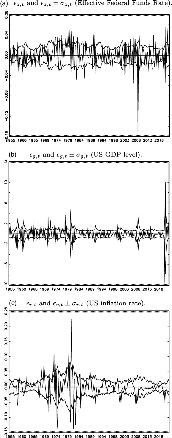
Figure 2. Evolution of $\epsilon _{t}$
and
$\epsilon _{t}$
and $\epsilon _{t} \pm \sigma _{t}$
for score-driven heteroskedastic
$\epsilon _{t} \pm \sigma _{t}$
for score-driven heteroskedastic $t$
-ABCD (1954 Q3 to 2022 Q1).
$t$
-ABCD (1954 Q3 to 2022 Q1).
Notes: $\sigma _{i,t}=\exp (\lambda _{i,t})[\nu/(\nu -2)]^{1/2}$
for
$\sigma _{i,t}=\exp (\lambda _{i,t})[\nu/(\nu -2)]^{1/2}$
for $i=z,g,r$
.
$i=z,g,r$
.
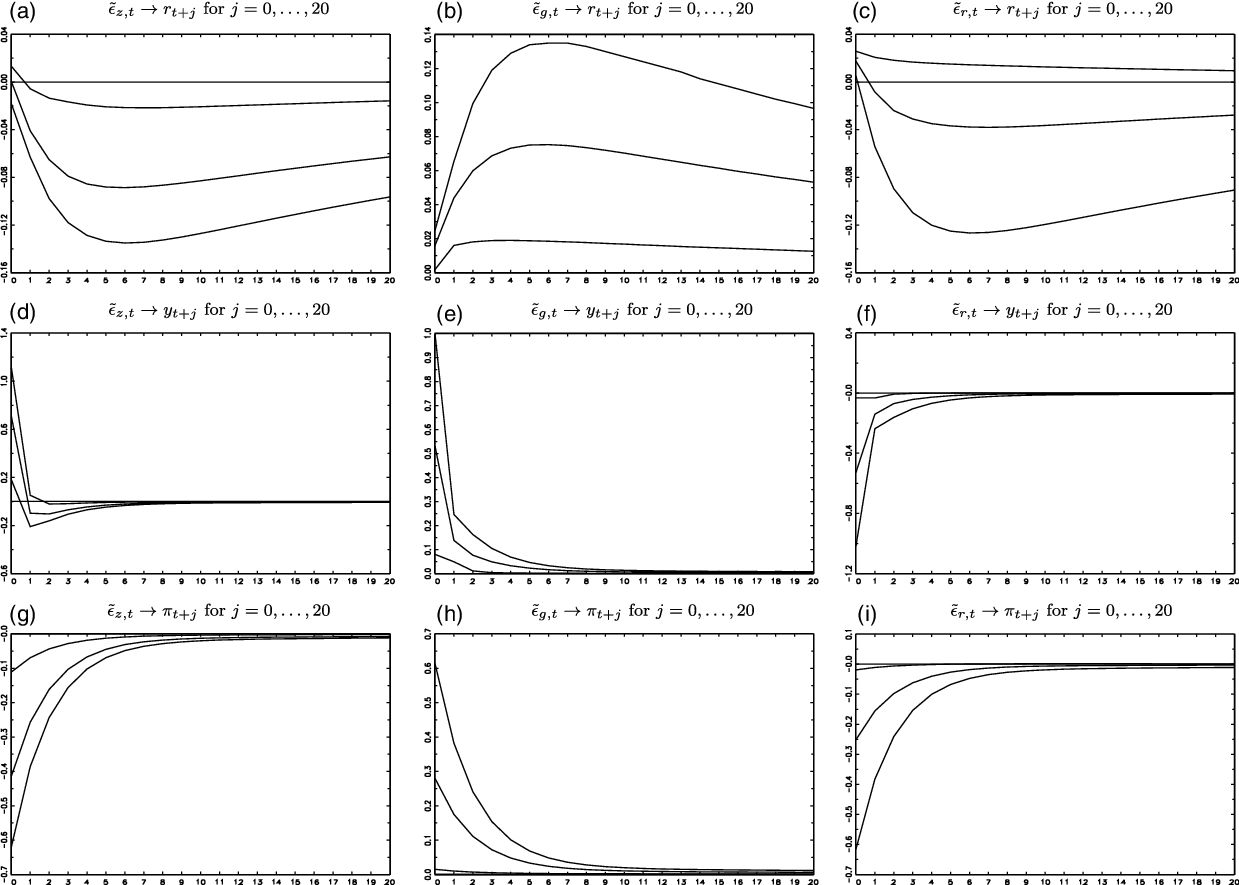
Figure 3. IRFs for the homoskedastic Gaussian-ABCD representation (5%, 50%, and 95% percentiles).
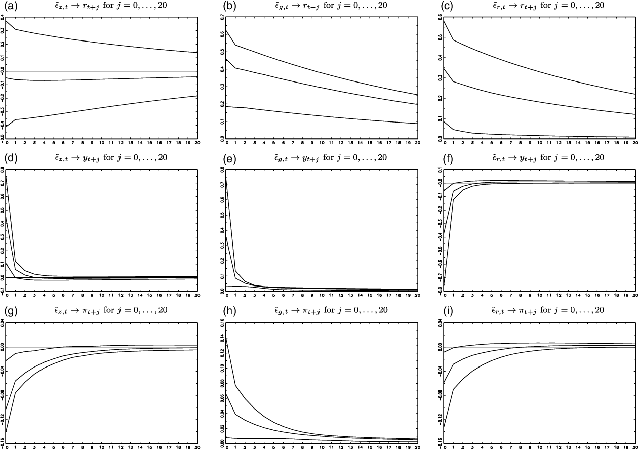
Figure 4. IRFs for the heteroskedastic score-driven $t$
-ABCD representation (5%, 50%, and 95% percentiles).
$t$
-ABCD representation (5%, 50%, and 95% percentiles).
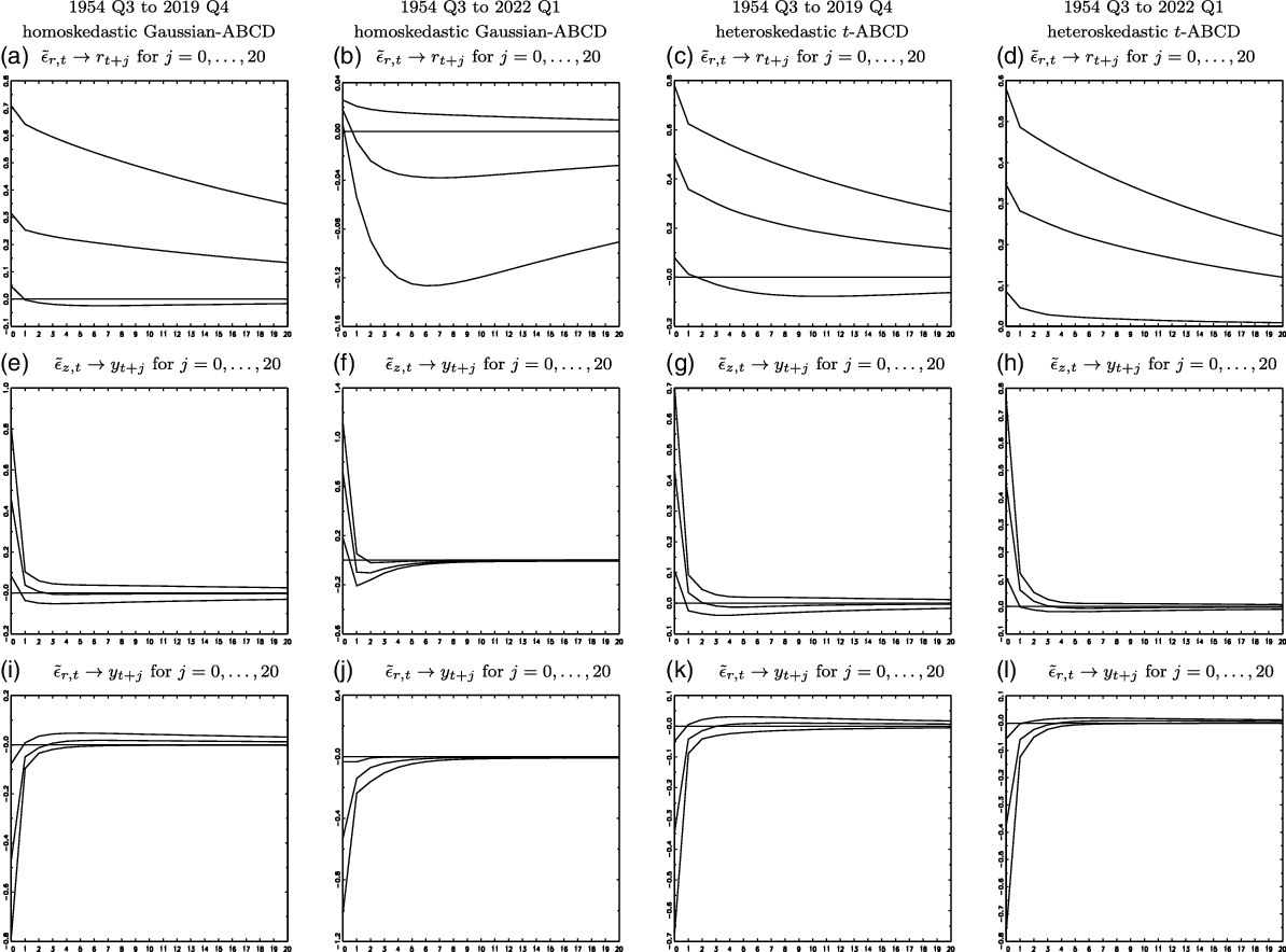
Figure 5. Comparison of IRFs estimates for the periods of 1954 Q3 to 2019 Q4 and 1954 Q3 to 2022 Q1 (5%, 50%, and 95% percentiles).
We highlight the following IRF results: First, the relatively low estimate of $\rho _{r}$
for the heteroskedastic ABCD representations, compared to the homoskedastic ABCD representations (Section 3.4), might be interpreted as a lower effect of an interest rate shock on subsequent interest rates, but, as is shown in Panel (c) of Figures 3 and 4, that is not the case. The persistence of interest rate shocks is similar for all ABCD representations [Panel (c) of Figures 3 and 4].
$\rho _{r}$
for the heteroskedastic ABCD representations, compared to the homoskedastic ABCD representations (Section 3.4), might be interpreted as a lower effect of an interest rate shock on subsequent interest rates, but, as is shown in Panel (c) of Figures 3 and 4, that is not the case. The persistence of interest rate shocks is similar for all ABCD representations [Panel (c) of Figures 3 and 4].
Second, a difference between the IRFs of the two ABCD representations, which may have policy implications, is in relation to the effects of an aggregate productivity shock on the US inflation rate $\tilde{\epsilon }_{z,t}\rightarrow \pi _{t+j}$
. For the homoskedastic Gaussian-ABCD representation,
$\tilde{\epsilon }_{z,t}\rightarrow \pi _{t+j}$
. For the homoskedastic Gaussian-ABCD representation, $\tilde{\epsilon }_{z,t}\rightarrow \pi _{t+j}$
is negative, and its contemporaneous value is
$\tilde{\epsilon }_{z,t}\rightarrow \pi _{t+j}$
is negative, and its contemporaneous value is $-0.41[-0.11,-0.62]$
[Panel (g) of Figure 3]. For the heteroskedastic
$-0.41[-0.11,-0.62]$
[Panel (g) of Figure 3]. For the heteroskedastic $t$
-ABCD representation,
$t$
-ABCD representation, $\tilde{\epsilon }_{z,t}\rightarrow \pi _{t+j}$
is also negative, but its effect is lower in absolute value, that is, its contemporaneous value is
$\tilde{\epsilon }_{z,t}\rightarrow \pi _{t+j}$
is also negative, but its effect is lower in absolute value, that is, its contemporaneous value is $-0.10[-0.02,-0.14]$
[Panel (g) of Figure 4].
$-0.10[-0.02,-0.14]$
[Panel (g) of Figure 4].
Third, another difference between the IRFs of different ABCD representations is in relation to the effects of government spending shocks on the US inflation rate $\tilde{\epsilon }_{g,t}\rightarrow \pi _{t+j}$
[Panel (h) of Figures 3 and 4]. For the homoskedastic Gaussian-ABCD representation,
$\tilde{\epsilon }_{g,t}\rightarrow \pi _{t+j}$
[Panel (h) of Figures 3 and 4]. For the homoskedastic Gaussian-ABCD representation, $\tilde{\epsilon }_{g,t}\rightarrow \pi _{t+j}$
is positive contemporaneously, and its value is
$\tilde{\epsilon }_{g,t}\rightarrow \pi _{t+j}$
is positive contemporaneously, and its value is $0.28[0.02,0.61]$
[Panel (h) of Figure 3]. For the heteroskedastic
$0.28[0.02,0.61]$
[Panel (h) of Figure 3]. For the heteroskedastic $t$
-ABCD representation,
$t$
-ABCD representation, $\tilde{\epsilon }_{z,t}\rightarrow \pi _{t+j}$
is also positive, but its effect is lower in absolute value, that is, its contemporaneous value is
$\tilde{\epsilon }_{z,t}\rightarrow \pi _{t+j}$
is also positive, but its effect is lower in absolute value, that is, its contemporaneous value is $0.07[0.01,0.14]$
[Panel (h) of Figure 4].
$0.07[0.01,0.14]$
[Panel (h) of Figure 4].
Fourth, another difference between the IRFs of different ABCD representations is in relation to monetary policy shocks, that is, effects of interest rate shocks on the US inflation rate $\tilde{\epsilon }_{r,t}\rightarrow \pi _{t+j}$
[Panel (i) of Figures 3 and 4]. For the homoskedastic Gaussian-ABCD representation,
$\tilde{\epsilon }_{r,t}\rightarrow \pi _{t+j}$
[Panel (i) of Figures 3 and 4]. For the homoskedastic Gaussian-ABCD representation, $\tilde{\epsilon }_{r,t}\rightarrow \pi _{t+j}$
is negative, and its contemporaneous value is
$\tilde{\epsilon }_{r,t}\rightarrow \pi _{t+j}$
is negative, and its contemporaneous value is $-0.25[-0.02,-0.61]$
[Panel (i) of Figure 3]. For the heteroskedastic
$-0.25[-0.02,-0.61]$
[Panel (i) of Figure 3]. For the heteroskedastic $t$
-ABCD representation,
$t$
-ABCD representation, $\tilde{\epsilon }_{r,t}\rightarrow \pi _{t+j}$
is also negative, but its effect is lower in absolute value, that is, its contemporaneous value is
$\tilde{\epsilon }_{r,t}\rightarrow \pi _{t+j}$
is also negative, but its effect is lower in absolute value, that is, its contemporaneous value is $-0.06[-0.01,-0.13]$
[Panel (i) of Figure 4].
$-0.06[-0.01,-0.13]$
[Panel (i) of Figure 4].
Fifth, as measured by the IRF confidence intervals, the estimation precision of the IRF for US GDP growth [Panels (d)−(f) of Figures 3 and 4] and US inflation rate [Panels (g)−(i) of Figures 3 and 4] is higher for the heteroskedastic score-driven $t$
-ABCD representation than for the homoskedastic Gaussian-ABCD representation. This indicates that the score-driven updates of the dependent variable may improve the statistical inferences of the impulse responses.
$t$
-ABCD representation than for the homoskedastic Gaussian-ABCD representation. This indicates that the score-driven updates of the dependent variable may improve the statistical inferences of the impulse responses.
Table 3. Sign restrictions on impact responses
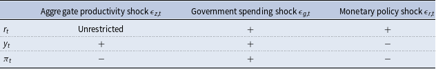
Finally, in Figure 5, we compare some of the IRF estimates for the homoskedastic Gaussian-ABCD representation and the heteroskedastic score-driven $t$
-ABCD representation, by using data for the periods of 1954 Q3 to 2019 Q4 and 1954 Q3 to 2022 Q1 (i.e., data without and with the COVID-19 pandemic, respectively). The IRF estimates show that the heteroskedastic score-driven
$t$
-ABCD representation, by using data for the periods of 1954 Q3 to 2019 Q4 and 1954 Q3 to 2022 Q1 (i.e., data without and with the COVID-19 pandemic, respectively). The IRF estimates show that the heteroskedastic score-driven $t$
-ABCD representation is robust to the COVID-19 pandemic, while for the homoskedastic Gaussian-ABCD representation some of the IRF estimates are significantly different for the two samples. These results indicate the robustness of the score-driven
$t$
-ABCD representation is robust to the COVID-19 pandemic, while for the homoskedastic Gaussian-ABCD representation some of the IRF estimates are significantly different for the two samples. These results indicate the robustness of the score-driven $t$
-ABCD representation to extreme observations.
$t$
-ABCD representation to extreme observations.
4. Conclusions
In this paper, we have introduced the heteroskedastic score-driven state-space model with Student’s $t$
-distributed innovations, and we have applied the new nonlinear model in an empirical macroeconomic way to a well-known DSGE model. In the heteroskedastic score-driven state-space model with Student’s
$t$
-distributed innovations, and we have applied the new nonlinear model in an empirical macroeconomic way to a well-known DSGE model. In the heteroskedastic score-driven state-space model with Student’s $t$
-distributed innovations, the coefficients are time-invariant and the error terms are conditionally heteroskedastic, similar to the best-performing model in Chan and Eisenstat (Reference Chan and Eisenstat2018).
$t$
-distributed innovations, the coefficients are time-invariant and the error terms are conditionally heteroskedastic, similar to the best-performing model in Chan and Eisenstat (Reference Chan and Eisenstat2018).
We have used the robust empirical macroeconomic model with time-varying conditional moments, to estimate a new heteroskedastic score-driven $t$
-ABCD representation of the DSGE model of An and Schorfheide (Reference An and Schorfheide2007). We have reported estimation results by using data on economic output, inflation, interest rate, government spending, aggregate productivity, and consumption of the USA for the period of 1954 Q3 to 2022 Q1. We found a superior statistical performance, lower policy-relevant effects, and a higher estimation precision of the IRF for US GDP growth and US inflation rate for the heteroskedastic score-driven
$t$
-ABCD representation of the DSGE model of An and Schorfheide (Reference An and Schorfheide2007). We have reported estimation results by using data on economic output, inflation, interest rate, government spending, aggregate productivity, and consumption of the USA for the period of 1954 Q3 to 2022 Q1. We found a superior statistical performance, lower policy-relevant effects, and a higher estimation precision of the IRF for US GDP growth and US inflation rate for the heteroskedastic score-driven $t$
-ABCD representation rather than for the homoskedastic Gaussian-ABCD representation. These results are due to the robustness of the heteroskedastic
$t$
-ABCD representation rather than for the homoskedastic Gaussian-ABCD representation. These results are due to the robustness of the heteroskedastic $t$
-QVAR model, even including the period of the COVID-19 pandemic and the start of the Russian invasion of Ukraine, which may motivate its practical use for empirical macroeconomic analysis.
$t$
-QVAR model, even including the period of the COVID-19 pandemic and the start of the Russian invasion of Ukraine, which may motivate its practical use for empirical macroeconomic analysis.
Supplementary material
To view supplementary material for this article, please visit https://doi.org/10.1017/S1365100522000712.
Acknowledgments
We are thankful for the comments and suggestions of the associate editor and referees of the journal, Juan Carlos Castañeda Fuentes, Matthew Copley, Andrew C. Harvey, and Jesús Fernández Villaverde. This paper was presented at the “Fifth Seminar of Economic Researchers” at the Bank of Guatemala in January 2021, at which the authors appreciate the discussion of Juan Carlos Catalán Herrera. All remaining errors are our own. The authors have no conflicts of interest to declare. Data and computer codes are available from the authors upon request. Szabolcs Blazsek and Adrián Licht acknowledge funding from Universidad Francisco Marroquín. Álvaro Escribano acknowledges funding from the Ministry of Economics of Spain (ECO2016-00105-001, MDM 2014-0431), the Community of Madrid (MadEco-CM S2015/HUM-3444), and Agencia Estatal de Investigación (2019/00419/001).


 Open access