

1. Introduction
The problem of how to segment continuous speech into components dates back at least to Harris (Reference Harris1955). Harris used “successor frequencies”, i.e., statistics, to predict boundaries between linguistic units, ideally morphemes. Saffran, Aslin, and Newport (Reference Saffran, Aslin and Newport1996) used syllable-based artificial languages to demonstrate that statistical information is indeed available for infants acquiring language. Results in language acquisition research indicate that speech segmentation is affected by various lexical and sublexical linguistic cues (see, e.g., Mattys, White, & Melhorn, Reference Mattys, White and Melhorn2005). Such cues can readily offer themselves as the base for various cognitive segmentation strategies. The distribution of strong and weak syllables, for instance, may help the language learner to use a metrical segmentation strategy (Cutler & Carter, Reference Cutler and Carter1987; Cutler & Norris, Reference Cutler and Norris1988), infants can possibly learn to use stress patterns for segmentation (Thiessen & Saffran, Reference Thiessen and Saffran2007), or they can exploit prosodic cues like lengthening, or rise in fundamental frequency of speech sounds (Bagou, Fougeron, & Frauenfelder, Reference Bagou, Fougeron and Frauenfelder2002).
Despite the diverse details that are known about the segmentation process (see Sonderegger, Reference Sonderegger2008, for a review), the question concerning the basic unit of segmentation is still open. Although the linguistic or psycholinguistic status of the syllable is rather complex (e.g., Bell & Hooper, Reference Bell, Hooper, Bell and Hooper1978; Cholin, Reference Cholin, Cairns and Raimy2011; Livingstone, Reference Livingstone2014) and a generally accepted precise definition is still lacking, it is widely assumed that an infant’s language acquisition is based on syllables (e.g., Mehler, Dupoux, & Segui, Reference Mehler, Dupoux, Segui and Altmann1990; Jusczyk, Friederici, Wessels, Svenkerud, & Jusczyk, Reference Jusczyk, Friederici, Wessels, Svenkerud and Jusczyk1993; Eimas, Reference Eimas, Goldstone, Scyhns and Medin1997). Syllable-based segmentation seems to be relevant for artificial languages (Saffran et al., Reference Saffran, Aslin and Newport1996), and for writing skills (Liberman, Shankweiler, Fischer, & Carter, Reference Liberman, Shankweiler, Fischer and Carter1974) as well.
Drienkó (Reference Drienkó, Takács, Varga and Vincze2016) proposed an algorithm for inferring boundaries of utterance fragments in relatively small unsegmented texts. The algorithm looks for subsequent largest chunks that occur at least twice in the text. The results were interpreted in terms of four precision metrics: Inference Precision, Alignment Precision, Redundancy, and Boundary Variability. In Drienkó (Reference Drienkó, Wallington, Foltz and Ryan2017a) the largest-chunk algorithm was used cross-linguistically to segment CHILDES utterances in four languages: English, Hungarian, Mandarin, and Spanish. The author found an Inference Precision range of 53.5%–65.6%, which grew when segments of specified lengths were merged. The unit for segmentation was the letter, i.e., the computer character, which can be regarded as a rough written equivalent of the speech sound. The advantage of the Largest Chunk method over other proposed segmentation strategies is that it allows direct quantitative results based solely on the linguistic structure of the given text without needing further cues like stress or metrical features. The strategy is in line with Peters’ (1983) approach to language acquisition, where the learner uses various cognitive heuristics to extract large chunks from the speech stream and the ‘ultimate’ units of language are formed by segmenting and fusing the relevant chunks.
The present study investigates whether the largest-chunk segmentation strategy can result in higher precision of boundary inference when syllables rather than characters are processed.Footnote 1 We do not distinguish between word or utterance boundaries. For the sake of direct comparison, we use the same data as Drienkó (Reference Drienkó, Wallington, Foltz and Ryan2017a), i.e., CHILDES texts in four languages: English (Anne, Manchester corpus; Theakston, Lieven, Pine, & Rowland, Reference Theakston, Lieven, Pine and Rowland2001), Hungarian (Miki, Réger corpus; Réger, Reference Réger1986; Babarczy, Reference Babarczy2006), Mandarin Chinese (Beijing corpus; Tardif, Reference Tardif1993, Reference Tardif1996), and Spanish (Koki, Montes corpus; Montes, Reference Montes1987, Reference Montes1992). Additionally, we segment two chapters from Gulliver’s Travels by Jonathan Swift in order to possibly detect text size effects. The length range of texts is 1,743–10,574 syllables, 5,499–43,433 characters.
After a short description of the algorithm in Section 2, we present our results in Section 3. This will be followed by a discussion and some conclusions in Sections 4 and 5, respectively.
2. Description of the algorithm
Our algorithm is basically identical with that of Drienkó (Reference Drienkó, Takács, Varga and Vincze2016, Reference Drienkó, Wallington, Foltz and Ryan2017a) except that there was an additional MERGE component included in that work. The basic, CHUNKER, module of the algorithm looks for subsequent largest syllable sequences that occur more than once in the text. Starting from the first syllable, it concatenates the subsequent syllables, and if a resultant string s i occurs in the text only once, a boundary is inserted before its last syllable since the previous string, s i–1, is the largest re-occurring one of the i strings. Thus the first boundary corresponds to s i–1, our first tentative speech fragment. The search for the next fragment continues from the position after the last character of s i–1, and so on.
The EVALUATE module computes four precision metrics: Inference Precision, Alignment Precision, Redundancy, and Boundary Variability. Inference Precision (IP) represents the proportion of correctly inferred boundaries (cib) to all inferred boundaries (aib), i.e., IP = cib / aib. The maximum value of IP is 1, even if more boundaries are inferred than all the correct (original) boundaries (acb). Redundancy (R) is computed as the proportion of all the inferred boundaries to all the correct (original) boundaries, i.e., R = aib / acb. R is 1 if as many boundaries are inferred as there are boundaries in the original text, i.e., aib = acb; R is less than 1 if fewer boundaries are inferred than acb; and R is greater than 1 if more boundaries are inferred than optimal. Alignment Precision (AP) is specified as the proportion of correctly inferred boundaries to all the original boundaries, i.e., AP = cib / acb. Naturally, the maximum value for AP is 1. Boundary Variability (BV) designates the average distance (in characters) of an inferred boundary from the nearest correct boundary, i.e., BV = (Σdfi) / aib. The above measures are not totally independent, since Inference Precision × Redundancy = Alignment Precision, but emphasise different aspects of the segmentation mechanism. Obviously, IP = AP for R = 1. The Largest-Chunk (LCh) segmentation algorithm is outlined in Table 1.
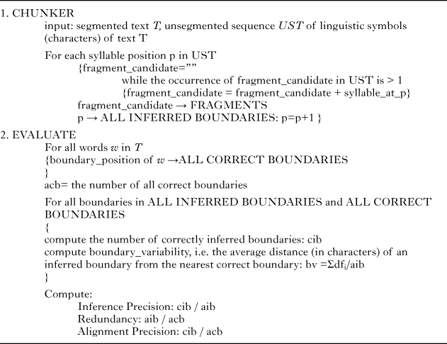
table 1. The Largest-Chunk Segmentation Algorithm
For some immediate insight, (1) illustrates how the arrangement of the individual elements in a sequence affect largest-chunk segmentation. Spaces correspond to inferred boundaries. Letters a, b, c, d, e, and f can also be seen as symbolising syllables.
- (1)
a) abcabc → abc abc
b) abcab → ab c ab
c) abc → a b c
d) abccba → a b c c b a
e) abcdefefcdab → ab cd ef ef cd ab
f) abcdefabcdef → abcdef abcdef
In (1b), for instance, the algorithm starts from the first a element, detects that a occurs twice in the sequence abcab, so takes the next element, b, detects that the corresponding segment, ab, occurs twice, proceeds to consider segment abc, detects that it occurs only once and infers a boundary after ab, the first largest ‘chunk’. Segmentation then continues from element c. Since c has only a single occurrence, a boundary should be inferred before it. However, this boundary has already been detected, so nothing happens and segmentation continues from the next position, a. Again, dual occurrence of a is detected, so segment ab is considered. As ab occurs twice, the algorithm should step to the next element. However, since b is the last element of the sequence, a boundary is inferred after it. Note that the inference of the last boundary is actually independent of the number of occurrences of the last segment. When an element occurs only once, a boundary is inserted before it and processing continues from the position immediately after it. As a result, any single-occurrence element is treated as a potential meaningful unit. An extreme example is given in (1c), where each element occurs only once. Recall that the LCh algorithm looks for largest re-occurring sequences, so single-occurrence units constitute a specific case. Arguably, regarding a single-occurrence sequence as a succession of its single-occurrence elements, rather than as a chunk itself, has the practical advantage of not missing any true boundary, and, perhaps more theoretically, it reflects our assumption that the ‘atomic’ segmentation elements are somehow – explicitly or implicitly – known to the segmenter.
Examples (1d–e) demonstrate a special case where symmetrical arrangement can effect ‘minimal largest chunking’. Each element in (1d) occurs twice, but there is no re-occurring combination of at least two elements, so a boundary is inferred at each position. This property of largest chunking can result in optimal segmentation for coupled elements. Suppose we have the ‘words’ ab, cd, and ef. If the input sequence is such that it contains each word twice, and the arrangement of letters/syllables is symmetrical, as in (1e) – a kind of ‘central embedding’ – a boundary will be inferred precisely after each word. In contrast, the largest chunks of (1f) conflate the three words.
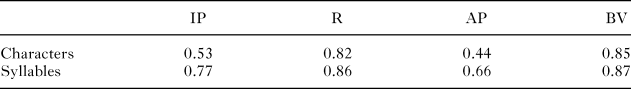
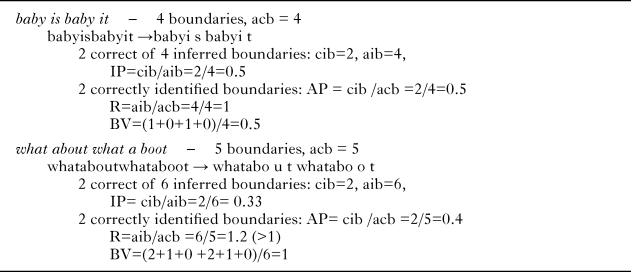
To see how precision values are calculated, consider two mini-sets of utterances, {baby is, baby it} and {what about, what a boot}. We provide a character-based analysis here, as summarised in Table 2, which will be contrasted with the syllable-based case in Section 4.
table 2. Calculating precision values (characters)

The baby is baby it text contains four word boundaries, thus acb = 4. The Largest-Chunk algorithm infers four boundaries corresponding to segments babyi, s, babyi, and t, which entails that aib = 4. Two of the four inferred boundaries are correct, cib = 2, resulting in Inference Precision IP = cib / aib = 2 / 4 = 0.5 and Alignment Precision AP = cib / acb = 2 / 4 = 0.5. Since the number of the inferred boundaries equals the number of the original boundaries, aib = acb, Redundancy is 1. The second and the fourth boundaries are correct, so their distance from the respective correct boundaries is zero, i.e., df2 = df4 = 0. If we shift the first inferred boundary one character to the left, we reach the first correct boundary, following baby. If we shift the first boundary one character to the right, we reach the second correct boundary, following is. Clearly, then, df1 = 1. Similarly, df3 = 1 as well, since by shifting the third inferred boundary one character either to the left or to the right, we reach the third or the fourth correct boundary, respectively. We compute Boundary Variability as BV = (df 1 + df 2 + df 3 + df 4) / aib = (1 + 0 + 1 + 0) / 4 = 0.5. Note that, when the distance of an inferred boundary is different for the left-side correct boundary and the right-side correct boundary, the shorter distance is chosen for df. Thus, for example, df1 = 2 for the what about what a boot text because the first inferred boundary, corresponding to whatabo is three characters away from the first correct left-side boundary, which follows what, and two characters away from the first correct right-side boundary, following about, so the right-side distance is chosen.
3. The experiments
In our experiments we used data from the CHILDES database (MacWhinney, Reference MacWhinney2000). All files were converted to simple text format, annotations were removed together with punctuation symbols and spaces. Hyphens were inserted after each syllable, so syllable, word, and utterance boundaries were indicated by hyphens. The segmentation problem consisted in differentiating word or utterance boundaries from word-medial syllable boundaries. Mother and child utterances were not separated, so the dataset for each language constituted an unsegmented (written) stream of ‘mother–child language’ represented as a single sequence of characters. The length range of the CHILDES texts was 1,743–9,021 syllables, 5,499–40,864 characters. Segmentation into syllables was done with the help of the Lyric Hyphenator (Juicio Brennan <http://juiciobrennan.com/hyphenator/>) for English, manually by the author for Hungarian, and the Spanish syllables were produced by the MARELLO.ORG syllabifier (<https://marello.org/tools/syllabifier/>). In the case of Chinese, syllable boundaries were understood as indicated by tone-marking numbers (1 to 4) and spaces in the pinyin transcript, so boundaries were inserted accordingly.
3.1. experiment 1 – English
In this experiment the first Anne file, anne01a.xml, of the Manchester corpus (Theakston et al., Reference Theakston, Lieven, Pine and Rowland2001) was analysed. The original text consisted of 374 utterances, 1,826 word tokens (acb), and 2,100 syllables. The unsegmented version of the text consisted of 8,899 characters. The segmentation algorithm inserted 1,133 boundaries (aib), of which 1,072 were correct (cib), thus Inference Precision = cib / aib = 0.946. The other precision values were as follows: Redundancy = 0.62, Alignment Precision = 0.59, Boundary Variability = 0.19. Table 3 contrasts the precision values with those obtained in Drienkó (Reference Drienkó, Wallington, Foltz and Ryan2017a), where the character was regarded as the primary segmentation unit. The data reveal that both Inference Precision and Alignment Precision are considerably higher for syllables, along with almost identical Redundancy values. The IP value approaching 1 (i.e., cib ≈ aib) entails that Redundancy (R = aib / acb) and Alignment Precision (AP = cib / acb) converge (0.62 vs. 0.59). The reduction of the Boundary Variability value indicates that the inferred boundaries are even closer to the correct ones in the case of syllables: on average, for an inferred boundary a correct boundary can be found within the distance of about 0.19 characters.
table 3. Precision values for Experiment 1 (Anne)

3.2. experiment 2 – Hungarian
The Hungarian data used in this experiment correspond with the miki01.xml file of the Réger corpus (Réger, Reference Réger1986; Babarczy, Reference Babarczy2006). The original text consisted of 589 utterances, 1,541 word tokens (acb), and 2,527 syllables. The unsegmented version of the text consisted of 9,358 characters. The segmentation algorithm inserted 1,324 boundaries (aib), of which 1,020 were correct (cib). The precision values were as follows: Inference Precision = cib / aib = 0.77, Redundancy = 0.86, Alignment Precision = 0.66, Boundary Variability = 0.87. Table 4 contrasts the precision values with those obtained in Drienkó (Reference Drienkó, Wallington, Foltz and Ryan2017a), where the character was regarded as the primary segmentation unit. The data reveal that both Inference Precision and Alignment Precision are higher for syllables, along with almost identical Redundancy values. Boundary Variability is slightly higher for syllables, although both values remain below 1.
table 4. Precision values for Experiment 2 (Miki)
3.3. experiment 3 – Mandarin Chinese
In this experiment we segmented Mandarin Chinese text included as bb1.xml in the Beijing corpus (Tardif, Reference Tardif1993, Reference Tardif1996). The file contains the pinyin transcription of the utterances. The original text consisted of 2,118 utterances, 7,064 word tokens (acb), and 9,021 syllables. The unsegmented version of the text consisted of 40,864 characters. The segmentation algorithm inserted 4,636 boundaries (aib), of which 4,271 were correct (cib). The precision values were the following: Inference Precision = 0.92, Redundancy = 0.66, Alignment Precision = 0.60, Boundary Variability = 0.34. Table 5 contrasts the precision values with the character-based results. It can be seen that both Inference Precision and Alignment Precision are higher for syllables, whereas Redundancy values are nearly the same. Boundary Variability is reduced by almost 50% for syllables.
table 5. Precision values for Experiment 3 (Beijing)

3.4. experiment 4 – Spanish
The Spanish data for this segmentation experiment came from the Koki material contained in the 01jul80.cha file of the Montes corpus (Montes, Reference Montes1987, Reference Montes1992). The original text consisted of 398 utterances, 957 word tokens (acb), and 1,743 syllables. The unsegmented version of the text consisted of 5,499 characters. The segmentation algorithm inserted 641 boundaries (aib), of which 521 were correct (cib). The precision values were the following: Inference Precision = 0.81, Redundancy = 0.67, Alignment Precision = 0.54, Boundary Variability = 0.54. Table 6 contrasts the precision values with the character-based results. It can be seen that both Inference Precision and Alignment Precision are higher for syllables, whereas Redundancy values are nearly the same. Boundary Variability is slightly higher for syllables.
table 6. Precision values for Experiment 4 (Koki)

3.5. experiment 5 – Gulliver
Switching from letters to syllables naturally reduces the number of linguistic units. For instance, the 8,899 characters of the English text in Experiment 1 represented 2,100 syllables. To have some insight on how the change in the number of processing units might affect segmentation precision in the case of the same language, we analysed an English text whose number of syllables is comparable to the number of characters in the Anne text of Experiment 1. We chose Chapters 1 and 2 from Gulliver’s Travels by Jonathan Swift. The two chapters were merged into a single text containing 7,765 word tokens, 238 utterances, and 10,574 syllables.Footnote 2 The unsegmented version of the text consisted of 43,433 characters. The segmentation algorithm inserted 6,078 boundaries (aib), of which 5,125 were correct (cib). The precision values were the following: Inference Precision = 0.84, Redundancy = 0.78, Alignment Precision = 0.66, Boundary Variability = 0.62. Table 7 contrasts the precision values with the character-based results. It can be seen that both Inference Precision and Alignment Precision are higher for syllables, whereas Redundancy values are nearly the same. Boundary Variability is lower for syllables. The quantitative results from all the experiments are summarised in Figure 1.
table 7. Precision values for Experiment 5 (Gulliver)

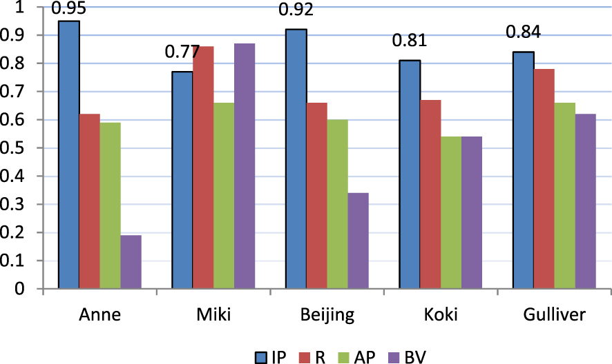
Fig. 1. Precision values for all the texts used in the segmentation experiments. (IP: Inference Precision; R: Redundancy; AP: Alignment Precision; BV: Boundary Variability)
4. Discussion
Our segmentation experiments allow the following observations:
1. Inference Precision is higher for syllables.
2. Redundancy is almost the same.
3. Alignment Precision is also higher for syllables.
4. When measured in characters, Boundary Variability can be both higher and lower for syllables – on average, it is lower – but the values stay below 1.
Let us consider these observations in more detail below.
1. The Inference Precision values are remarkably higher for syllables. The 53%–66% IP value range, averaging 59%, for characters rose to 77%–95%, averaging 86%, in the case of syllables (cf. Table 8).
2. Redundancy is almost the same for characters and for syllables – although slightly higher for syllables (cf. Table 9). The average R value is 3% higher in the case of syllables. This means that switching to syllables as basic segmentation units does not notably change the proportion of inferred boundaries. It is perhaps worth noting that the R values stay below 1, i.e., fewer boundaries are inserted than would be required by the original segmentation, by the number of words in the original texts.
3. Alignment Precision is higher for syllables (cf. Table 10). The 41% average of AP values for letters became 61% in the case of syllables. This is the consequence of the relation AP = IP × R and the fact that R is about the same for characters and syllables. If IP is greater for syllables, then multiplying by about the same R entails that AP will be greater as well. In other words, if a larger proportion of the inferred word boundaries is correct for syllables than for letters, then a larger proportion of the original boundaries will be detected correctly for syllables if the same percentage of boundaries is inserted as for letters.
4. The Boundary Variability values do not show a consistent pattern. They can be both higher and lower for syllables – on average, they are 16% lower (cf. Table 11). However, the values stay below 1, which means that for any inferred boundary a correct boundary can be found within the average distance of less than one character, i.e., a correct boundary can be reached by shifting the boundary less than one character, on average, to the left or to the right.
table 8. IP values across texts
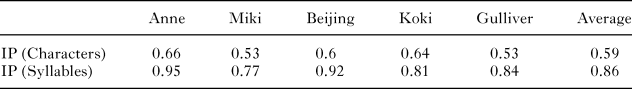
table 9. R values across texts
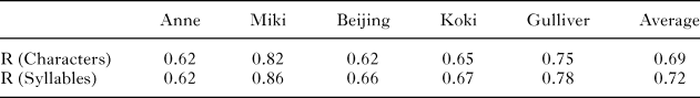
table 10. AP values across texts
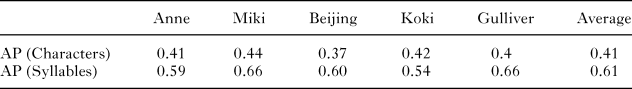
table 11. BV values across texts
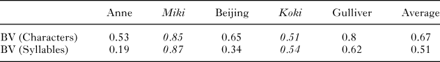
Note that we measured Boundary Variability in characters, not in syllables. We believe that this gives a more precise picture of the segmentation process since syllables can vary in length, and they are composed of letters/phonemes anyway. However, Table 12 displays BV values measured in syllables as well (cf. the BV(syllables)s row). The data show that BV is much lower when measured in syllables: a correct boundary can be reached by shifting the incorrect boundary 0.148 syllables, on average, to the left or to the right. Table 12 also illustrates that a rough estimate for Boundary Variability in terms of syllables can be calculated by dividing the BV value measured in characters (first row of Table 12) by the average syllable length for the given text (third row). See ‘Appendix’ for an explanation.
table 12. Details for measuring BV in syllables
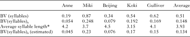
[*] Recall that syllable ends are marked by hyphens in the texts to be segmented, so in reality each syllable is 1 character shorter than in our texts. Naturally, this is also true for the averages in the table.
To illustrate the basic information gain effected by the transition to syllables from characters, consider the examples of Table 2 (repeated here as Table 13).
table 13. Calculating precision values (characters)
The Largest Chunk segmentation algorithm possibly inserts boundaries syllable-medially as, e.g., babyi exemplifies. Such errors are naturally ruled out in syllable-based segmentation: no boundary can be inserted into the smallest unit. As a consequence, we see an increase in precision values. In the case of the ba-by-is-ba-by-it text, for example, all boundaries are correct, which amounts to 100% Inference Precision, all the other values being optimal (cf. Table 14).
table 14. Calculating precision values (syllables)
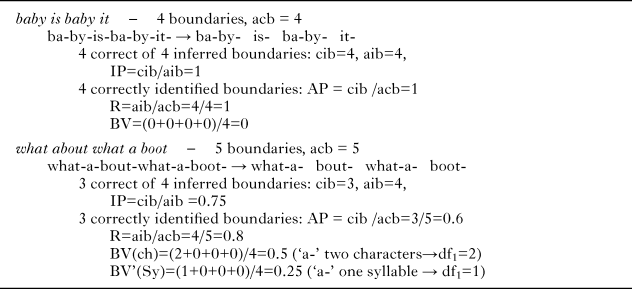
On the other hand, the syllable-based LCh algorithm still may undesirably infer word-medial syllable boundaries. For instance, the first inferred boundary, after what-a- in the what-a-bout-what-a-boot- text is incorrect since it divides a-bout- into two. Such errors reduce the effectiveness of segmentation. This is demonstrated by the what-a-bout-what-a-boot- example where Inference Precision cannot reach 100%, i.e., IP = 0.75. Nevertheless, the 0.75 value constitutes a considerable increase from 0.33 in the character-based case. Tables 15 and 16 illustrate that the change in precision metrics due to switching from characters to syllables is fairly similar for our current examples and for our experiments. Besides the IP values there is an increase in Alignment Precision. The BV values become lower for syllables whether measured in characters or in syllables (values in brackets). Recall that in the experiments BV values became unambiguously lower only when they were measured in syllables. Redundancy values are the same for the {baby is baby it} text but for the {what about what a boot} text they show a decrease, contrary to the experimental results. This may underline, on the one hand, that our toy examples are not capable of capturing all aspects of the segmentation mechanism, and/or, on the other hand, that Redundancy is somehow more independent of the sort of information gain which our examples were designed to visualise.
table 15. Precision values for the ‘baby is baby it’ example
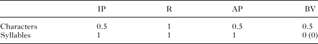
table 16. Precision values for the ‘what about what a boot’ example

5. Conclusions
The present study examined how various precision metrics are affected by a transition from characters to syllables in applying the Largest-chunk method to text segmentation. The data show an increase in Inference Precision, as well as in Alignment Precision. Redundancy is almost the same, while a reduction in Boundary Variability can be observed, which is more unambiguously pronounced when measured in syllables. Nevertheless, BV remains below 1 even when measured in characters. Overall, our quantitative results seem to underline the role of the syllable, as opposed to the letter or speech sound, in text segmentation using the Largest-chunk strategy. Conversely, our results indicate that the strategy might serve as an insightful component for a model of speech segmentation.
We did not attempt to explain the differences in precision values for the different texts. That would be an exciting topic for further research. Clearly, on the one hand, segmentation must be affected by typological differences between languages, but, on the other hand, idiosyncratic parameters of a given text, such as length, genre, register, speaker, etc., may also play a role. Research on infant word segmentation suggests that extraction of target words is facilitated when they are aligned with utterance boundaries (Seidl & Johnson, Reference Seidl and Johnson2006; Johnson, Seidl, & Tyler, Reference Johnson, Seidl and Tyler2014). Such findings would make it reasonable to investigate how LCh segmentation would be affected by information on utterance boundaries.
Appendix
We show that for text T, consisting of L characters, k syllables, Boundary Variability in terms of syllables can be estimated by dividing the BV value measured in characters by the average syllable length for the given text. Recall we calculate BV as in (A1), where n = aib (all inferred boundaries) and df i denotes the distance of the i-th inferred boundary from the nearest correct boundary.
 $${\rm{BV = }}{1 \over n}\sum\nolimits_{i = 1}^n {df_i } $$
We write Δf for the sum, as in (A2).
 $${\rm{BV = }}{1 \over n}\sum\nolimits_{i = 1}^n {df} _i = {1 \over n}\Delta f$$
Suppose Δf contains kΔ syllables with average syllable length s, i.e., (A3) holds.
 $$\Delta f{\rm{ = k}}_\Delta \times s,\,\,\,s = {{\Delta f} \over {k_\Delta }}$$
Assume that the distribution of syllable length in sum Δf is the same as for the whole text T, entailing the equality of average syllable length for Δf with the average syllable length for the whole text, as expressed in (A4).
 $$s = {{\Delta f} \over {k_\Delta }} = {L \over k}$$
Writing (A4) for s in (A3) we get (A5), and writing (A5) for Δf in (A2) we get (A6).
 $$\Delta f = k_\Delta \times s = k_\Delta {{\Delta f} \over {k_\Delta }} = k_\Delta {L \over k}$$
 $${\rm{BV = }}{{\rm{1}} \over n}\Delta f{\rm{ = }}{1 \over n}k_\Delta {{\Delta f} \over {k_\Delta }}{\rm{ = }}{1 \over n}k_\Delta {L \over k}$$
 We can approximate BV in syllables if we change the ‘length scale’ by choosing average syllable length  ${L \over k}$ as unit length, i.e., by dividing (A6) by s. Thus Equation (A7) can be used for approximating BV’, Boundary Variability measured in syllables, when BV is known.
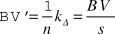 $$BV' = {1 \over n}k_\Delta = {{BV} \over s}$$


