


1. Introduction
In most industrialized countries, population aging generates a need for policy reforms and adjustments in retirement systems (OECD, 2017). Here, evidence-based policy decisions demand reliable causal analyses. This study exploits two natural experiments with respect to early retirement rules. We offer causal evidence on the behavioral adjustments induced by retirement entry age reforms for German men. In particular, we investigate how shifts in retirement entry age affect labor force participation and program substitution.
The retirement entry age is central to the fiscal challenges facing retirement insurances. In most retirement systems, the rules for retirement entry are complex and allow for different types of adjustments. Often, there are regulations for specific groups of the workforce. As an example, the German retirement system uses different retirement entry regimes (so-called ‘pathways’ to retirement), e.g., for females, those with disabilities or severe handicaps, and those who are unemployed prior to retirement with different retirement entry ages. Many reforms modified these ages to respond to challenges associated with population aging. While the differentiation of pathways into retirement is relevant in most retirement systems (OECD, 2017), the international literature rarely discusses this feature of institutional settings.
A large literature investigates the causal effects of a variety of specific retirement reforms. A first group of contributions considers structural parameters and separates wealth and accrual effects (e.g., Hanel, Reference Hanel2010, Reference Hanel2012; Brown, Reference Brown2013; Atalay and Barrett, Reference Atalay and Barrett2015). A second group chooses a reduced form approach to determine causal reform effects on individual labor force status. Here, some analyses study reforms of the normal retirement age (NRA) (Mastrobuoni, Reference Mastrobuoni2009; Hanel and Riphahn, Reference Hanel and Riphahn2012; Lalive and Staubli, Reference Lalive and Staubli2015) which provides retirement benefits without actuarial deductions. Others consider modifications of the early retirement age (ERA) (Staubli and Zweimüller, Reference Staubli and Zweimüller2013; Cribb et al., Reference Cribb, Emmerson and Tetlow2016; Hernæs et al., Reference Hernæs, Markussen, Piggott and Røed2016; Manoli and Weber, Reference Manoli and Weber2018; Geyer et al., Reference Geyer, Haan, Hammerschmid and Peters2020) at which retirement is possible only with reduced benefits.Footnote 1
We contribute to this literature in three important ways: First, we improve on a strategy to identify causal effects first introduced by Krueger and Pischke (Reference Krueger and Pischke1992) (for applications see Mastrobuoni, Reference Mastrobuoni2009; Hanel and Riphahn, Reference Hanel and Riphahn2012). The strategy identifies causal effects of cohort-specific reforms by comparing the behavior of treated younger and non-treated older birth cohorts at given ages. The identifying assumption is that absent the reform the developments over the lifecycle would have been identical across cohorts. We use a weaker identifying assumption by additionally considering behavioral differences for affected (male) and non-affected (female) individuals of the same age and birth cohort. Our difference-in-difference-in-differences (DIDID) estimation accounts for general trends across cohorts as well as for specific trends across cohorts for the male and female subsamples. We show that in our case this yields slightly more conservative estimates than the traditional DID approach.
Second, we exploit two reforms of the NRA and ERA within the same retirement pathway. This generates insights beyond those available from using just one reform. Staubli and Zweimüller (Reference Staubli and Zweimüller2013, p. 20) point out that ‘a rise in the ERA is likely to be a more effective measure to increase LFP among older workers as opposed to a rise in the NRA’. We offer a comparison of these responses.
Third, we study the response of male workers to reforms of retirement age regulations. This adds to a recent literature which looked at the effects of similar reforms for females: Geyer and Welteke (Reference Geyer and Welteke2021) apply a regression discontinuity approach to investigate German female workers' response to the abolition of an ERA. They differentiate active and passive substitution patterns and find that women mostly stay passive in their respective labor market status after a reform rather than actively moving to substitute states.Footnote 2 Engels et al. (Reference Engels, Geyer and Haan2017) investigate women's response to an increase in the NRA in the case of Germany. They also do not find much active substitution, e.g., into disability retirement. Oguzoglu et al. (Reference Oguzoglu, Polidano and Vu2020) study an increase of the eligibility age to the means-tested age pension for women in Australia with comparable results. Lalive et al. (Reference Lalive, Staubli and Magesan2020) recently confirmed that the majority of Swiss females simply adjust their retirement choices to perceived norms of retirement instead of maximizing the payout of retirement benefits when they are confronted with an increase of the NRA.
We take advantage of large samples of potential retirees using administrative data from the German mandatory retirement insurance. We use the start of benefit receipt as a precise measure of retirement entry which allows us to separately identify reform effects on labor market exit and retirement entry behaviors. These data provide more reliable evidence than prior survey-based studies (e.g., Krueger and Pischke, Reference Krueger and Pischke1992; Atalay and Barrett, Reference Atalay and Barrett2015; Giesecke, Reference Giesecke2018). The data also allow us to investigate a broad set of labor market responses and study program substitution. Besides causal reform effects on employment and unemployment, we identify the reforms' effects on alternative pathways into retirement. This is important because the reform objective – reducing the fiscal burden of aging populations – cannot be reached if individuals respond by simply shifting to different retirement programs.
In terms of identification, our study is most similar to Atalay and Barrett (Reference Atalay and Barrett2015) who investigate the effects of the 1993 Australian Age Pension reform. That reform progressively increased the ERA for women from 60 to 65 between 1995 and 2014. The authors study the effects on labor force participation and program substitution and find strong effects in both dimensions. They identify causal effects using difference-in-differences (DID) estimations on affected birth cohorts for men and women. In addition, they present their DID estimates separately by age following Mastrobuoni (Reference Mastrobuoni2009), but without specifying a full DIDID model. In a review of the Atalay and Barrett (Reference Atalay and Barrett2015) analysis, Morris (Reference Morris2022) points out that after controlling for diverging time trends in the treatment and control groups the effect declines in size and turns insignificant. As Atalay and Barrett (Reference Atalay and Barrett2015), we identify the causal effect comparing males and females. However, we focus our analysis on treatment effects using a full DIDID model; thus, in our analysis identical time trends for male and female birth cohorts are not required as long as age-specific trends agree. Therefore our analysis is robust to the issues pointed out by Morris (Reference Morris2022). Also, while in the Australian pension program changes in labor force participation do not yield accrual effects on social security wealth and benefit receipt is means tested, we consider a more traditional retirement insurance with accrual and without means tests. Finally, we differ from Atalay and Barrett (Reference Atalay and Barrett2015) and also Mastrobuoni (Reference Mastrobuoni2009) by using precise information on benefit receipt from administrative data instead of approximating the timing of retirement based on self-reported non-participation in the labor force. Similar to these prior studies and as suggested by the literature (e.g., Coile, Reference Coile2004; Atalay et al., Reference Atalay, Barrett and Siminsky2019), our measure of reform effects might be downward biased, if the reform generated spillover effects within couples.
In terms of institutions, our study is most similar to Engels et al. (Reference Engels, Geyer and Haan2017) who investigate a reform of the retirement pathway for females in Germany. That reform consisted of a stepwise increase of the NRA from age 60 to 65 for the birth cohorts of 1940 and after in combination with the contemporaneous introduction of an ERA and related benefit deductions. Engels et al. (Reference Engels, Geyer and Haan2017) study the direct effect of benefit discounts and consider a set of outcomes following Mastrobuoni (Reference Mastrobuoni2009). They find sizeable employment and retirement responses to the introduction of benefit deductions. In contrast, we focus on reforms of the unemployment pathway to retirement which affected men: about 30% of the relevant cohorts used the pathway (DRV, 2018). Our first reform, announced in 1996 and effective 1997, increased the NRA stepwise from age 60 to 65 for the birth cohorts of 1937 and after and contemporaneously introduced an ERA with related benefit deductions. Our second reform, announced in 2004 and effective 2006, increased the ERA stepwise from age 60 to 63 for the birth cohorts 1946 and after. We differ from Engels et al. (Reference Engels, Geyer and Haan2017) by first, considering reform effects on additional outcomes, second, by focusing on men instead of women, third by offering an additional control group in our identification strategy, and finally, by comparing the effects of two separate reforms.
We find that both reforms increase the propensity to stay employed longer, postpone unemployment, and delay old-age retirement. After reform 1 (NRA), we observe an increased use of substitute pathways to enter retirement, i.e., disability retirement and retirement of the severely handicapped. Thus, our sample of men actively changed their labor force status in response to financial incentives. This differs from findings for women by Engels et al. (Reference Engels, Geyer and Haan2017) and Geyer and Welteke (Reference Geyer and Welteke2021). While the direction of the reform effects is similar after both reforms, the magnitude of behavioral adjustments after reform 2 (ERA) appears to be larger. The results are robust but slightly larger when only a DID strategy is applied. The fiscal effects of both reforms are positive for social insurances and the taxpayer. This is consistent with the national and international literature. We find that individuals who have little time to adjust to the reform and who are caught by surprise delay retirement by more and adjust employment more strongly than those who have time to prepare for regulatory changes. The reform effects vary by pension wealth: in response to financial incentives the poorest prolong employment and postpone retirement by more than those with higher pension wealth.
In Section 2, we describe the institutional features of the German retirement system and discuss our hypotheses and the underlying mechanisms of the expected reform effects. Section 3 outlines our data, sample, and variables, and provides first descriptive evidence. Additionally, we discuss the empirical method and potential challenges to the identification strategy. Results and robustness tests follow in Sections 4 and 5, and Section 6 concludes.
2. Institutional background and hypotheses
2.1 Retirement insurance and pathways to retirement
The German retirement insurance operates on a pay as you go basis. It is funded mostly by mandatory contributions of employers and employees. Regulated at the federal level, it covers more than 80% of the population, excluding only civil servants and the self-employed. It offers old-age, disability, and survivor benefits. Given the limited relevance of private pensions in Germany, the mandatory retirement system provides the main source of income for most elderly households (Frommert, Reference Frommert2010).Footnote 3
Generally, benefit amounts depend on amounts and years of contribution. More specifically, the benefit formula considers the sum of annual ‘earning points’. The earning points for 1 year represent the ratio of the individual's earnings and the mean earnings of all insured persons, i.e., the relative individual annual contribution. An individual who contributed to the retirement insurance over 45 years based on the annual average earnings would receive a gross benefit that amounts to about 48% of gross earnings (BMAS, 2019). Benefit eligibility is regulated along pathways to retirement. Examples for such pathways are retirement ‘due to unemployment’, ‘for women’, ‘after long term employment’, or ‘disability retirement’. Pathways can be used with an NRA or an ERA. With the ERA, the minimum retirement entry age and subsequent benefit amounts are lower than that with the NRA; specifically, each month of early benefit receipt prior to the NRA generates a permanent benefit cut by 0.3% (i.e., 3.6% for each full year).
We exploit two reforms of the entry age for the unemployment pathway into retirement. The unemployment pathway into retirement has been available for blue and white collar workers since 1957. The utilization of the pathway increased over successive birth cohorts. It was used by 10% of all retired men born in 1925, 24% of those born in 1935, and 30.8% of those born in 1940. For subsequent birth cohorts the shares declined, e.g., to 19.7% for the 1945 cohort (see DRV, 2018, p. 93).Footnote 4
The pathway was used particularly by individuals with low reemployment probabilities, who had lost their jobs in the wake of structural changes in firms and industries and whose occupational experience was no longer demanded in regional labor markets (Mika and Krickl, Reference Mika and Krickl2020). However, at the same time these individuals had accumulated substantial claims against the retirement insurance. Their past earnings and retirement benefits often exceeded those of the average retiree (DRV, 2018).
The first reform increased the NRA stepwise from age 60 to 65 starting with individuals born in January 1937 and ending with those born in December 1941 (see column 1 of Table 1 and Figure A.1 in the Appendix). At the same time, early retirement with benefit deductions became newly available at age 60 for all cohorts. The second reform increased the ERA stepwise from age 60 to 63 starting with individuals born in January 1946 and ending with those born in December 1948.Footnote 5 Both reforms contained regulations to protect the ‘legitimate expectation’ (Vertrauensschutz) of individuals.Footnote 6
Table 1. Age at retirement by pathway and birth cohort

Notes: For a more complete description see Table A.1. The entry ‘rising to’ means that the retirement age increased by 1 month for each month of birth in the relevant birth cohort: in column 1 individuals born, e.g., in January of 1937 had an NRA of 60 and 1 month, those born in February of 1937 had an NRA of 60 and 2 months and so on, reaching an NRA of 61 years for those born in December of 1937.
Source: SGB VI, BMAS (2017), Steffen (Reference Steffen2018), and own calculations.
Column 2 of Table 1 depicts the retirement pathway for women (see also Figure A.1).Footnote 7 Here, the reform for birth cohorts 1940 and after is very similar to the first reform of the unemployment pathway. In addition to these two pathways, the ‘regular old-age’ retirement pathway has traditionally been available at age 65 and does not offer an ERA; ‘retirement after long-term employment’ is available for individuals with 35 insurance years and offers an ERA of 63 and an NRA of 65. A special pathway is available for individuals with severe handicaps. Finally, the disability pathway used to provide retirement benefits independent of age (Hanel, Reference Hanel2012). It is available until the ‘regular old-age’ retirement age is reached.Footnote 8
As retirement insurance contributions paid in East Germany were in part treated differently from those paid in West Germany, we follow Ye (Reference Ye2019) and use only individuals who contributed in West Germany. In robustness tests, we include individuals with labor market experience in East Germany.
Since anticipation behavior can affect the estimation of treatment effects, it is important to consider reform announcements: in 1989, a reform law was passed which stipulated that starting in 2001 retirement entry ages should start to increase toward age 65 beginning with the 1941 birth cohort (Steffen, Reference Steffen2018). However, in 1996 and 1997, reforms accelerated the increase in the retirement age and brought the starting date of these retirement entry age adjustments forward from 2001 to 1997. This newly affected individuals of the 1937 (instead of 1941) birth cohort (reform 1), who had little time for adjustment as they turned age 59 in 1996.
The ERA had been available since 1997 for birth cohorts 1937 and after. In 2004, a law was passed which mandated that the minimum age for early retirement on the unemployment pathway increased starting in 2006 (reform 2) (Steffen, Reference Steffen2018). As both reforms were passed into law very briefly before they became effective, we expect to observe short-term behavioral adjustments that are not yet attenuated through anticipatory behavior changes.
2.2 Related institutions: unemployment as a bridge to retirement
As we focus on retirement after unemployment, it is important to describe unemployment insurance (UI) rules. Historically, two types of unemployment benefits were provided: an insurance-based payment (UB I) that covered about 60% of last net earnings and a means tested system which provided a more modest minimum income support (UB II). The duration of UB I benefit payment depends on the number of UI contribution years and the age of the unemployed individual and was reformed several times (see Table A.3).
Since the 1990s, it was common practice to use the long unemployment benefit duration as a bridge to retirement: retirement benefits after unemployment were available starting at age 60 without benefit deductions. So workers who were laid off starting e.g., at the age of 57 and 4 months, received UI benefits for up to 32 months, and then entered retirement after unemployment. In our analysis, we follow Engels et al. (Reference Engels, Geyer and Haan2017) and account for changes in the duration of unemployment benefit payout by controlling for the individual and age-specific maximum entitlement length.
2.3 Expected reform effects and hypotheses
The first reform increased the NRA in a stepwise fashion and introduced an ERA. The second reform increased the ERA stepwise and thus disallowed retirement at early ages. The first reform implied a negative shock to individuals' social security wealth and the second reform restricted individuals' choice sets by making early retirement unavailable.
Under the first reform, it remained possible to retire starting at age 60. However, the reform introduced a benefit reduction after early retirement which increased over subsequent birth cohorts. To retire at age 60, the 1936 birth cohort did not suffer benefit reductions, cohort 1937 had to forgo up to 3.6%, and cohort 1942 and later lost 18% of their benefits.
The literature offers different theoretical frameworks to derive hypotheses with respect to the reforms' effects. The first is based on an intertemporal consumption model. In this view, the reforms generated income and substitution effects: the income effect consists of the decline in ‘pathway-specific pension wealth’, e.g., at age 60. The newly introduced additional reduction in pension benefits that follows each month by which retirement takes place prior to the new NRA increases the price of leisure. This generates the substitution effect in the choice of entering the unemployment pathway (for a more formal description, see, e.g., Hanel and Riphahn, Reference Hanel and Riphahn2012). If leisure is a normal good, both effects reduce the demand for leisure and increase labor force attachment and incentives to postpone retirement entry. We therefore expect prolonged employment and unemployment. In particular, workers who would have used unemployment as a bridge into retirement before age 60 without the reform may postpone unemployment to later ages: their unemployment may decline before age 60 and increase afterward. Also, we expect delayed retirement entry after the first reform. Since the reduction in pension benefits vary by cohort and by age, the income and substitution effects should differ across birth cohorts and for every cohort by age.
Alternative pathways of retirement, e.g., for those with severe handicaps, continued to offer retirement entry at age 60 without benefit deductions for the birth cohorts 1937–39. In addition, disability retirement was available without any age restrictions at full benefits for the 1937 cohort. For the birth cohorts 1938 and after, disability retirement at full benefits was available until December 31, 1999. For subsequent entries, benefit discounts were introduced if the retiree had not yet reached age 63 (see Table A.2). Individuals may have used these alternative pathways as substitute exit routes out of the labor force.
The second reform abolished the option to use ERA on the unemployment pathway prior to age 63 in a stepwise fashion for birth cohorts 1946 and after. This reform may have no lifecycle income effects if prior benefit discounts after early retirement were actuarially fair. Nevertheless, behavioral adjustments will follow from changes to age-specific budget constraints: if the pathway to early retirement is unavailable other labor market options are more attractive as they provide an income. The effect of increasing ERA has been looked at for different countries before: see, e.g., Cribb et al. (Reference Cribb, Emmerson and Tetlow2016) for the UK, Staubli and Zweimüller (Reference Staubli and Zweimüller2013) for Austria, Vestad (Reference Vestad2013) studied the effect of a reduced ERA for Norway, and Geyer and Welteke (Reference Geyer and Welteke2021) and Geyer et al. (Reference Geyer, Haan, Hammerschmid and Peters2020) studied different pathways in Germany. These studies generally find that such a reform (a) affects employment and unemployment, and (b) incentivizes program substitution.
A second framework to explain retirement behavior has recently been developed by Seibold (Reference Seibold2021). He uses the example of 644 pension benefit continuities in Germany to establish convincing evidence that financial incentives alone cannot explain retirement patterns. Instead, he suggests that NRA and ERA become reference points for individual retirement decisions. Under this framework, the two reforms considered here shifted the reference points for retirement entry after unemployment which should then yield similar adjustment patterns.
Overall, we expect that after both reforms individuals stay in employment longer (H1). Because unemployment as a bridge to retirement becomes less attractive, after reform 1 (NRA), unemployment may decline prior to age 60 and increase at age 60 and after. In contrast, after reform 2 (ERA), unemployment may decline at age 60 and after because retirement without deductions was available only at age 65. In sum, we expect that unemployment is postponed to later ages (H2). We expect that both reforms contributed to a delay in the utilization of the unemployment pathway to retirement because it became either more expensive (reform 1) or inaccessible (reform 2) (H3). Also, we expect that the demand for alternative pathways, such as disability retirement or retirement for the severely handicapped, increased (H4).
In addition, we compare the responses of two reforms. Staubli and Zweimüller (Reference Staubli and Zweimüller2013) suggest that responses to changes in the ERA are larger than responses to changes in the NRA: while individuals can ignore changes in the NRA by accepting reduced benefit payments upon retirement postponements of the ERA must be heeded. We compare the responses to reforms 1 and 2, which affect the same pathway but affect different birth cohorts.
3. Data and methods
3.1 Data
We use administrative data offered by the German Pension Insurance. The Versicherungskontenstichprobe (VSKT) provides roughly a 1% random sample of persons aged 15–67 and covered by the German Statutory Pension Insurance. The data are available annually since 2002.Footnote 9 Each wave provides information on demographic and pension relevant characteristics such as year and month of birth, nationality, information on monthly labor market status and earning points (Himmelreicher and Stegmann, Reference Himmelreicher and Stegmann2008; Stegmann, Reference Stegmann2008).
We use different samples for the two reforms. They consist of men and women born between 1935–39 and 1945–48. Due to special pension rules, we do not consider civil servants, self-employed, miners, and persons with pension entitlements according to the law on foreign pensions (FRG).Footnote 10
We analyze the reform effects by comparing the labor market behavior of treated and non-treated individuals. We compare the birth cohorts 1937–39 and 1946–48 who are affected by the reforms to the cohorts 1935–36 and 1945 who are not affected. In addition, we take advantage of the fact that females who are eligible for the female retirement pathway are basically not affected by the reform of the unemployment pathway.Footnote 11 Therefore, they constitute a control group in our analyses. The female retirement pathway provides an NRA of 60 for birth cohorts potentially affected by our first reform (1935–39) and an ERA of 60 for those birth cohorts potentially affected by our second reform (1945–48). Since the female birth cohorts 1940–44 were affected by the NRA reform for female retirement (see Table 1), we do not use these cohorts and thus limit our post-reform cohorts for reform 1 to 1937–39 and our pre-reform cohorts for reform 2 to 1945.Footnote 12 For reform 1 (NRA), we therefore consider individuals born 1935–39 and for reform 2 (ERA) individuals born 1945–948.
To obtain comparable subsamples, we follow Engels et al. (Reference Engels, Geyer and Haan2017) and consider only those men and women in our sample who fulfill the eligibility criteria for the female retirement pathway when they are at age 55.Footnote 13 These eligibility criteria demand a waiting period of 15 years and a compulsory contribution period of at least 10 years after reaching age 40. Clearly, we cannot condition on the eligibility criteria of the unemployment pathway since this involves the potentially endogenous response of anticipatory unemployment.
For every birth cohort, we use one wave of the VSKT to avoid duplicate observations.Footnote 14 Based on the biographical information, we code monthly observations for each individual from age 60 plus 0 months to age 62 plus 11 months. As discussed above some individuals are not affected by the reform because of regulations to protect their ‘legitimate expectation’. We code the treatment status of those individuals, about 2% of the sample, as not treated. Overall, we use 11,240 different individuals and 404,640 person-month observations for the first and 8,566 individuals and 308,376 person-month observations for the second reform.Footnote 15
Our dependent variables characterize five different states. They describe for every age month whether an observation is in ‘employment’, ‘unemployment’, ‘old-age retirement’, ‘severely handicapped retirement’, or ‘disability retirement’. ‘Old-age retirement’ combines retirement entries through all pathways except for ‘severely handicapped retirement’, or ‘disability retirement’.Footnote 16
Table 2 describes our dependent variables. In the sample for reform 1, 21% of the full sample are in employment, about 4% in unemployment, 57% of the person-month observations of 60–62 years olds are already in old-age or severely handicapped retirement, and about 13% in disability retirement.Footnote 17 The reform 2 sample has higher shares in employment and unemployment and a lower share in retirement.
Table 2. Descriptive statistics of dependent variables
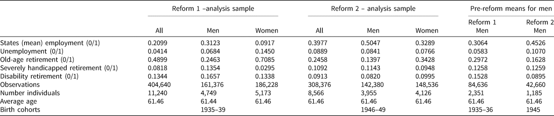
Notes: All observations are in the age range 60–62. Old-age retirement combines retirement after all pathways except for severely handicapped retirement and disability retirement; given our age restrictions this comprises only the two pathways of retirement due to unemployment and retirement for women (see Table A.1). Tables A.5–A.8 describe all variables and provide further descriptive statistics. The number of observations in the columns entitled ‘All’ exceed the sum of male and female observations because sampling restrictions with respect to the protection of ‘legitimate expectations’ are not yet imposed in the columns ‘All’ (see Sections 2.1 and 3.1 in the text). The affected observations are dropped from the male subsamples described in the columns entitled ‘Men’.
Source: SUFVSKT2002_FAU_Schrader-SUFVSKT2013_FAU_Schrader, own calculations.
Figures 1 and 2 depict cohort- and gender-specific employment, unemployment, and old-age retirement behavior by age for both reforms. Figure 1a shows employment rates by age for men and women of cohorts 1935–39 (we dropped some birth cohorts to enhance clarity). After age 60, employment drops for men and women. However, males stay in employment longer than females. As expected, the treated male cohorts 1937 and 1939 have higher employment rates than the pre-reform cohort 1935 with little difference across cohorts for females. The developments for the non-affected cohorts are similar for males and females supporting our strategy to use females as a control group. Figure 1b presents unemployment rates by cohort, gender, and age. While these rates are rather similar for females across birth cohorts, the male rates clearly reflect the reform incentives: the unemployment rate of post-reform cohorts exceeds that of pre-reform cohorts at almost all age months. The effect is most visible at the early ages. The male and female developments for the pre-reform cohorts are parallel. Figure 1c depicts old-age retirement starting at age 60. Generally, males' retirement rates are lower than females'. While male cohorts affected by the reform have lower old-age retirement rates than the pre-reform cohorts this does not hold for females, matching expectations. As before, females and males in the cohort not affected by the reform (1935) have similar age patterns.

Figure 1. (a) Reform 1 (NRA) – Employment rate by age, cohort, and gender. (b) Reform 1 (NRA) – unemployment rate by age, cohort, and gender. (c) Reform 1 (NRA) – old-age retirement rate by age, cohort, and gender.
Notes: The NRA for birth cohorts 1935 was 60; the NRA for birth cohorts 1937 (1939) increased in monthly steps from 60 to 61 (62 to 63) for those born from January through December. The ERA did not exist for birth cohort 1935; for birth cohorts 1937 and after it was at 60. For the figures, we deleted male, post-reform cohort observations who due to protection of legitimate expectation (measured as of age 60) were not treated by the reforms. We show the gender-specific number of individuals of a given birth cohort and age in employment relative to the number of all individuals in that gender, age, and birth cohort cell in our sample. Source: SUFVSKT2002_FAU_Schrader-SUFVSKT2013_FAU_Schrader, own calculations.

Figure 2. (a) Reform 2 (ERA) – employment rate by age, cohort, and gender. (b) Reform 2 (ERA) – unemployment rate by age, cohort, and gender. (c) Reform 2 (ERA) – old-age retirement rate by age, cohort, and gender.
Notes: The ERA for birth cohort 1945 was 60; the ERA for birth cohorts 1946 (1948) increased in monthly steps from 60 to 61 (62 to 63) for those born from January through December. The NRA was 65 for all birth cohorts. For the figures, we deleted male, post-reform cohort observations who due to protection of legitimate expectation (measured as of age 60) were not treated by the reforms. We show the gender-specific number of individuals of a given birth cohort and age in employment relative to the number of all individuals in that gender, age, and birth cohort cell in our sample. Source: SUFVSKT2002_FAU_Schrader-SUFVSKT2013_FAU_Schrader, own calculations.
Figure 2 present the same outcomes with respect to reform 2, for cohorts 1945–48 (cohort 1947 omitted to enhance clarity). Figure 2a shows similar employment-age patterns for males and females pre-reform (i.e., birth cohort 1945). For the cohorts affected by the reform, we find substantial changes in employment rates for men, but not for women. The unemployment rates in Figure 2b are unclear which is likely related to reforms of unemployment benefit duration in 2006 and 2008 for which we do not control here.Footnote 18 However, the male pre-reform cohort stands out. Also, we find a drop in unemployment rates at the early ages and an increase in later ages for cohort 1948, as expected. Finally, Figure 2c shows retirement rates and confirms cohort and gender differences: the retirement of the treated male cohorts declines stepwise by age and birth cohort which follows exactly the incentives generated by reform 2. As in Figure 1c, we observe a similar age pattern for the male and female pre-reform cohort.
Figures 1 and 2 show that affected and non-affected male birth cohorts differ in their employment, unemployment, and retirement behavior in agreement with the expected reform effects. Female birth cohorts are suitable controls as they show similar pre-reform patterns.
3.2 Empirical methods
We aim to identify the causal effect of two reforms on retirement behavior and labor force participation choices of older workers. We exploit the fact that both reforms affected specific birth cohorts at specific ages, e.g., reform 1 modified the NRA of individuals age 60 and born in 1937 or later and reform 2 modified the ERA of individuals age 60 and born in 1946 or later. Based on the combination of birth cohort and observation period, we can identify the causal reform effect if we assume that the reform is the only determinant of possible behavior changes across birth cohorts at a given age. This identification strategy is widely applied in the literature and requires that there are no changes in age-specific cohort trends absent the reform (e.g., Mastrobuoni, Reference Mastrobuoni2009; Hanel and Riphahn, Reference Hanel and Riphahn2012; Staubli and Zweimüller, Reference Staubli and Zweimüller2013).
We can go beyond this standard approach and allow for age-specific cohort trends. We additionally compare groups of men treated by the reform and women not treated by the reforms, both, at ages when the reform was effective or not, and for birth cohorts which were and were not affected. This DIDID setting is possible because the change in the unemployment pathway to retirement was not accompanied by a similar and simultaneous change in the retirement pathway for females and because the changes were implemented stepwise by cohort.
Under the requirements of the female retirement pathway, women continued to be able to retire at an NRA of 60 after our reform 1 (NRA) and similarly to use an ERA of 60 after our reform 2 (ERA) (see Table 1). Thus, we distinguish men who are affected by the reform (treatment group) from women who are not affected (control group) and compare their behavioral choices at ages which were affected and ages that were not affected by the reforms for birth cohorts affected (post-reform) and not affected (pre-reform) by the reforms. We calculate the reform effect as the difference in changes between men and women across ages and cohorts. This identifies causal effects if the behavioral adjustments across cohort groups and genders would have been identical for different ages without the reform. This is a weaker identifying assumption than that required for a DID model: we can allow for changes in the labor market affecting men and women differently across birth cohorts as long as they are not age-specific.
The recent literature intensely discusses spillover effects in retirement choices of couples. There is substantial evidence showing coordination in spouses' retirement choices (e.g., Hospido, Reference Hospido2015; Atalay et al., Reference Atalay, Barrett and Siminsky2019). Clearly, such coordination behavior can modify the policy reforms' effects as changes of the retirement entry age for men affects the behavior of women and vice versa. If spillovers are neglected in the analysis of reform effects, the results can be biased downward (see Coile, Reference Coile2004). Besides the direct reform effects of increasing retirement entry ages on the husbands' retirement, the reform could induce indirect reform effects by increasing the wives' retirement ages, as well. Since we compare male and female labor market outcomes and as our data do not allow us to control for the spouses' labor market choices our overall impact assessment of the reform may be biased downward.
Let men indicate whether the individual is male (men = 1) or female and belongs to the control group (men = 0). C contains month and year of birth fixed effects and post is equal to one for cohorts affected and equal to zero for cohorts not affected by the reform. A represents the individuals' monthly age in a given monthly observation a. Some ages are affected by the reform and others are not; age (valued 0 or 1) indicates whether an individual is affected by the reform in a given month. X are individual level control variables; we use measures of past earnings, health, tenure, and insurance group indicators (blue collar, white collar, other) as of age 55, i.e., prior to the observation window. Finally, to account for unemployment and disability benefit reforms (see Sections 2.1 and 2.2), we also control for the maximum length of (potential) unemployment benefit receipt and the month- and person-specific potential discount after disability retirement.Footnote 19 We use the following linear regression model:

We estimate the parameters β, γ, and θ using least-squares regression, where γ represents the causal effect of interest. ɛ is a random error. Note that the triple interaction term is identical to using an indicator for being affected by the reform versus not (see, e.g., the specification by Staubli and Zweimüller, Reference Staubli and Zweimüller2013). We consider variations of this specification where we control for a post reform indicator instead of the detailed date of birth fixed effects, C.
In addition to the interaction model 1, we apply specifications that control for the reform intensity for given individuals (see Duggan et al., Reference Duggan, Singleton and Song2007, for a related approach). Appendix Tables A.9 and A.10 describe the number of months of benefit discounts after reform 1 (NRA) and the number of months by which an early retirement must be postponed after reform 2 (ERA). We use these indicators of reform intensity (I) that vary at the cohort, gender, and age level in a separate specification and estimate the following model for both reforms:Footnote 20

The estimate for γ yields the causal reform effect. As before, we apply alternative specifications which use a simple post reform indicator instead of monthly date of birth fixed effects, C. Generally, γ is identified by the reform which changed the incentives jointly by age and cohort. In the case of reform 1 (NRA), intensity represents the magnitude of the benefit discount that follows upon immediate retirement for reform 2 (ERA) it represents the waiting time to ERA. As we are not conditioning our sample on meeting the unemployment pathway criteria, our estimates represent intention to treat (ITT) effects. We report robust standard errors that are clustered at the individual level.
4. Results and robustness
4.1 Reform effects
Table 3 shows the estimated causal effects of reform 1 (NRA) for the five labor force states of those aged 60–62. Columns 1–3 present the estimations based on the interaction model (equation (1)) using different controls. The sign of the estimated reform effects agree with our expectations: we find increased employment and unemployment, reduced old-age retirement, and increased use of substitute pathways into retirement, i.e., disability and severely handicapped retirement.
Table 3. Reform 1 (NRA) – treatment and treatment intensity effects for the labor force states
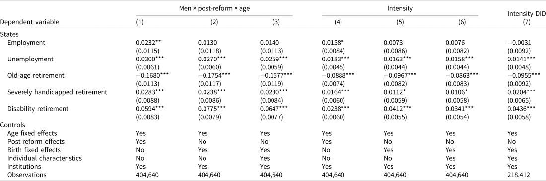
Notes: The table shows OLS estimates of the coefficient on ‘men × post-reform × age’ in columns 1–3 and on intensity in column 4–7. In addition to reported controls, all specifications except for column 7 include an indicator for men. Columns 1 and 4 use interactions of ‘post-reform’ and age fixed effects. Columns 2, 3, and 5–7 additionally control for interaction effects of age with birth fixed effects and columns 2, 3, 5, and 6 also for interaction effects of age effects and men and birth effects and men. Column 7 shows the results of DID estimation without females as a control group. Table A.5 describes all controls. Individual level-clustered standard errors (SE) in parentheses. *p < 0.1, **p < 0.05, ***p < 0.01.
Source: SUFVSKT2002_FAU_Schrader-SUFVSKT2013_FAU_Schrader, own calculations.
The results in columns 4–6 use precise measures of reform 1 intensity (equation (2)) based on individuals' age and birth cohort (see Table A.9). The results are mostly statistically significant and confirm the patterns in columns 1–3. More specifically and based on column 6, they suggest that 1 year of postponed normal retirement increases the propensity to be employed in any given month by 0.8 percentage points (insignificantly) and the propensity to be unemployed by 1.6 percentage points; based on the pre-reform means (see last columns of Table 2) this amounts to increases in employment and unemployment by 2.6% and 27%, respectively. It reduces the propensity of old-age retirement by 8.6 percentage points, i.e., 28.9%, and yields large and significant increases in the propensity to use substitute retirement pathways in total by more than 4 percentage points per month, an increase by 16.0%.
We apply identical procedures to analyze the effects of reform 2 (ERA). Table 4 shows the estimates. In columns 1–3, we find large and significant increases in the propensity to be employed and declines in the propensity to be unemployed. As expected, the propensity for old-age retirement declines. Surprisingly, we do not observe a significant increase in the use of substitute retirement pathways. In the case of disability retirement, this may be connected to the 1999 reform and the connected benefit discounts (see Section 2.1). The negative effect on severely handicapped retirement could be explained by an earlier reform of this pathway.Footnote 21 The estimation results based on the intensity measure (columns 4–6) confirm these findings.
Table 4. Reform 2 (ERA) – treatment and treatment intensity effects for the labor force states
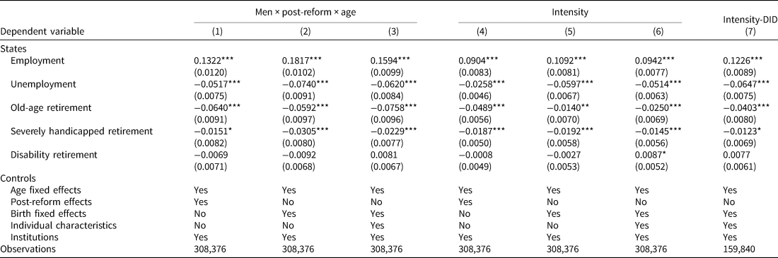
Notes: The table shows OLS estimates of the coefficient on ‘men × post-reform × age’ in columns 1–3 and on intensity in columns 4–7. In addition to reported controls, all specifications except for column 7 include an indicator for men. Columns 1 and 4 use interactions of ‘post-reform’ and age fixed effects. Columns 2, 3, and 5–7 additionally control for interaction effects of age with birth fixed effects and columns 2, 3, 5, and 6 also control for interaction effects of age effects and men and birth effects and men. Column 7 shows the results of DID estimation without females as a control group. Table A.6 describes all controls. Individual level-clustered SE in parentheses. *p < 0.1, **p < 0.05, ***p < 0.01.
Source: SUFVSKT2002_FAU_Schrader-SUFVSKT2013_FAU_Schrader, own calculations.
In column 7 of Tables 3 and 4, we show the results of DID analyses where we omitted females as a control group. Here, the causal effect is identified by comparing men of given ages across birth cohorts, only. For both reforms, the findings are generally robust in terms of sign and significance of the estimates. However, the magnitude of the effects is generally larger when female control groups are disregarded (compare columns 6 and 7). Thus, using female control groups provides conservative estimates of effects which otherwise may have been overstated.
Finally, we compare the effect size of the two reforms. We argued based on Staubli and Zweimüller (Reference Staubli and Zweimüller2013) that the effect of reform 2 should exceed that of reform 1 because the former is more strict and renders, e.g., an early retirement at age 60 impossible instead of merely expensive. It may be misleading to simply compare coefficient estimates across reforms because the estimates represent ITT effects. They are estimated for the population of potential retirees that might consider the unemployment pathway and do not account for the share of individuals who will actually be unemployed and affected by the reform. Therefore, we adjust the estimated effects based on the observed share (p) of individuals in pre-reform cohorts that either used the NRA (prior to reform 1) or the ERA (prior to reform 2) of the unemployment pathway. Out of all men born in 1935 or 1936 (1945) in our sample, 29.7% (16.3%) used the unemployment pathway prior to age 63. The ratio of the ITT estimates over p yields estimates of the average treatment effect of the treated (ATT) (see Angrist and Pischke, Reference Angrist and Pischke2009) which is appropriate if p does not vary substantially over time. Table 5 restates the estimation results of column 6 of Tables 3 and 4. Columns 3 and 4 of Table 5 present the ATT after dividing by p. As the ATT estimates scale the ITT estimates by factors 3.4 (column 3) and 6.1 (column 4) they show that the response of those actually affected by the reform are 3 and 6 times as large as the ITT estimates shown before. As an example, the propensity to be employed in a given month increases by 2.6 and 57 percentage points for those treated by a 1 year change in the NRA and ERA, respectively. The resulting estimates for employment (both positive) and unemployment (in absolute terms) are substantially larger for reform 2. The negative effects on old-age retirement are larger for reform 1 than for reform 2. Based on the sum of the effects on all three retirement pathways (old-age, severely handicapped, and disability retirement), reform 2 reduced the overall propensity to be in retirement by more than reform 1.
Table 5. Reforms 1 (NRA) and 2 (ERA) – comparison of the treatment intensity effects
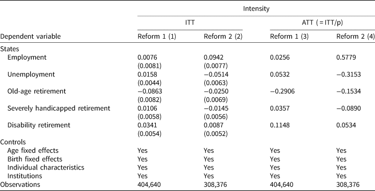
Notes: The table shows OLS estimates of the coefficient on intensity. In addition to reported controls, all specifications include an indicator for men and control for interaction effects of age and birth fixed effects and for interaction effects of age effects and men and birth effects and men. All controls for reform 1 (NRA) are described in Table A.5 and for reform 2 (ERA) in Table A.6. In column 3 we use p = 0.297 as the share of all men born in 1935 or 1936 in our sample who used the unemployment pathway prior to age 63; in column 4 we use p = 0.163 as the share of all men born in 1945 who used the unemployment pathway prior to age 63.
Source: SUFVSKT2002_FAU_Schrader-SUFVSKT2013_FAU_Schrader, own calculations.
4.2 Threats to identification
We offer several tests to investigate whether our identifying assumption holds. In columns 2 and 5 of Table 6, we add linear time trend controls to the main estimation for both reforms separately for males and females. Generally, our main results (repeated in columns 1 and 4) are robust. In columns 3 and 6, we control for a richer specification of a linear trend; we add its interaction with the men indicator, post-reform cohort indicators, the interaction of men and post-reform indicator, and also with the interaction of men, post-reform, and affected age indicator. Again, the main results hold up. Therefore, time trends do not drive our main results.
Table 6. Reforms 1 and 2 – treatment intensity effects with controls for time trends and placebo estimation

Notes: The table shows OLS estimates of the coefficient on intensity in columns 1–6 and on ‘men × post-reform × age’ in column 7. In addition to reported controls, all specifications include an indicator for men and all control for interaction effects of age and birth fixed effects and for interaction effects of age effects and men and birth effects and men. For a description of all controls see Tables A.5 and A.6. Individual level-clustered SE in parentheses. *p < 0.1, **p < 0.05, ***p < 0.01.
*Placebo reform is set so that cohort 1935 is pre-reform and cohort 1936 is only post-reform cohort.
Source: SUFVSKT2002_FAU_Schrader-SUFVSKT2013_FAU_Schrader, own calculations.
In column 7 of Table 6, we show placebo results for reform 1 (NRA), where we consider the birth cohort 1935 as control and cohort 1936 as treated by reform 1. The results confirm that a non-existing reform had no significant effects which supports our setting.Footnote 22
4.3 Heterogeneities
We study effect heterogeneities along two dimensions. First, we distinguish the reform effects by year of birth, and separately estimate our models for the relevant birth cohorts. We expect that both reforms caught the oldest cohorts by surprise. Younger cohorts had more time to adjust after the reform laws were passed. The results for reform 1 (NRA) and 2 (ERA) in columns 2–4 of Tables 7 and 8 show that the reform effect was indeed strongest for the oldest, most surprised cohorts.Footnote 23
Table 7. Reform 1 (NRA) – heterogeneity of treatment intensity effects
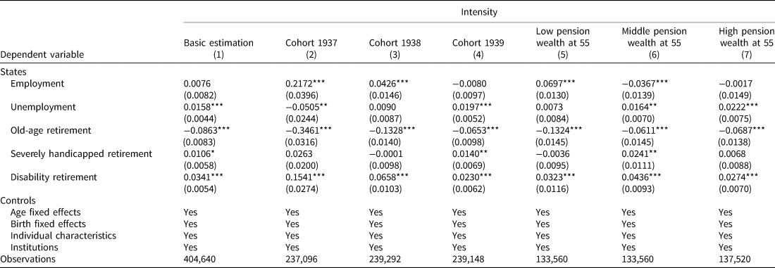
Notes: The table shows OLS estimates of the coefficient on intensity. All specifications are as in column 6 of Table 3. All controls are described in Table A.5. Individual level-clustered SE in parentheses. *p < 0.1, **p < 0.05, ***p < 0.01.
Source: SUFVSKT2002_FAU_Schrader-SUFVSKT2013_FAU_Schrader, own calculations.
Table 8. Reform 2 (ERA) – heterogeneity of treatment intensity effects

Notes: The table shows OLS estimates of the coefficient on intensity. All specifications are as in column 6 of Table 4. All controls are described in Table A.6. Individual level-clustered SE in parentheses. *p < 0.1, **p < 0.05, ***p < 0.01.
Source: SUFVSKT2002_FAU_Schrader-SUFVSKT2013_FAU_Schrader, own calculations.
Next, we study the heterogeneity of reform effects along the pension wealth distribution. We group individuals based on their earning points at age 55 representing individual pension wealth. As the reform introduced relative benefit deductions (e.g., by 3.6%), all retirees were affected identically in relative terms, independent of pension wealth. We consider three wealth tertiles of similar size (separately for males and females) and show the estimates in columns 5–7 of Tables 7 and 8 for reforms 1 and 2. We expect that individuals with low pension wealth are most susceptible to potential benefit cuts whereas high wealth individuals may more easily forgo a small fraction of benefits to take advantage of early retirement. The same pattern would result if those with low pension wealth are more likely to actually use the unemployment pathway. The findings mostly agree with our expectations: after both reforms, those with the lowest pension wealth increased employment the most.Footnote 24 Also, they show the largest decline in old-age retirement entry after both reforms.
It is informative to compare the reforms: while reform 1 yielded the expected statistically significant employment and unemployment effects only for the oldest, most surprised cohort, after reform 2 the estimates for employment and unemployment are statistically significant for all cohorts. Similarly, the estimated employment and unemployment effects across pension wealth tertiles vary in sign and significance for reform 1 but are relatively large and statistically significant for reform 2. This confirms that reform 2 yielded stronger behavioral responses and affected the entire treatment group.
4.4 Robustness tests – sampling issues
In Table 9, we show the estimation results for both reforms for different samples. In columns 2 and 5 we add those male observations who would not have been eligible for female retirement at age 55. In columns 3 and 6, we add those observations who had accumulated some employment spells in East Germany. In both cases, our main results (columns 1 and 4) hold up to these changes in the sample with only a few exceptions.
Table 9. Reforms 1 and 2 – treatment intensity effects when adding non-eligible men and those with East German spells and when omitting observations in January–March 2006
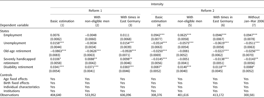
Notes: The able shows OLS estimates of the coefficient on intensity. All specifications are as in column 6 of Tables 3 and 4. Specification in column 2 and 5 include an indicator for eligibility and specification in column 3 and 6 an indicator for times in East Germany. For a description of all controls for reforms 1 and 2 see Tables A.5 and A.6, respectively. Columns 2 and 5 add observations on men to the baseline sample who failed to meet the eligibility requirements of female retirement. Columns 3 and 6 add those observations on men and women to the baseline sample who at some point earned pension points in East Germany. Column 7 omits observations from January 1 to March 31 2006. Individual level-clustered SE in parentheses. *p < 0.1, **p < 0.05, ***p < 0.01.
Source: SUFVSKT2002_FAU_Schrader-SUFVSKT2013_FAU_Schrader, own calculations
In our specifications for reform 2, we account for the 2006 reform of the German UI by controlling for the individual and age-specific maximum entitlement length (see Section 2.2). Riphahn and Schrader (Reference Riphahn and Schrader2020) and Dlugosz et al. (Reference Dlugosz, Stephan and Wilke2014) show that the reform generated substantial anticipation behavior in terms of earlier unemployment entries. In order to evaluate whether this affects our results, we re-estimated the main specification after omitting observations from January to March of 2006. The results in column 7 of Table 9 show that our findings are robust to this change.Footnote 25
4.5 Robustness tests – continuous long run outcome measures
For a different perspective and to investigate effects before retirement age, we consider summary measures of individual labor force states over time. Based on precise biographical information, we use the number of months an individual spent in our five states in three different age ranges (57–59, 60–62, and 57–62) as continuous dependent variables.Footnote 26 We apply a DID analysis to our data with one cross-sectional observation per person instead of monthly outcomes. Therefore, we cannot control for monthly age fixed effects and have to adjust the definition of some control variables (for details see Tables A.11 and A.12).Footnote 27 However, for this analysis it is possible to illustrate the parallel paths which we depict in Figures A.2–A.6. The figures provide evidence that the common trend assumptions hold and we can claim to establish causal effects. For reform 2, we cannot show similar graphs because we have only one pre-reform birth cohort.
Table 10 shows estimates of the reform effect based on the specifications of column 6 in Tables 3 and 4. After reform 1, we observe an increase in the number of months spent in employment for all age groups. Unemployment declined substantially before age 60 and increased after age 60 with a large negative overall effect. We also find the expected decline in the number of months in old-age retirement. At the same time, the number of months spent in severely handicapped retirement and disability retirement increased significantly for all age groups. After reform 2, we observe increases in the number of months in employment, declines in unemployment for all age groups, reduced old-age retirement, and severely handicapped retirement. Among those aged below 60, we find modest but statistically significant substitution into disability retirement. Overall, the patterns are similar to those in response to reform 1.Footnote 28
Table 10. Reforms 1 (NRA) and 2 (ERA) – treatment intensity effects for the number of months in labor force status
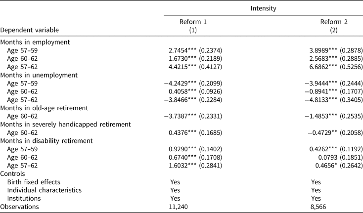
Notes: The table shows OLS estimates of the coefficient on intensity in columns 1 and 2. In addition to reported controls, all specifications include an indicator for men. All controls are described in Table A.10. Individual level-clustered SE in parentheses. *p < 0.1, **p < 0.05, ***p < 0.01.
Source: SUFVSKT2002_FAU_Schrader-SUFVSKT2013_FAU_Schrader, own calculations.
5. Discussion
Based on reform 1 (NRA), we found that for those aged 60–62 postponing the NRA by 1 year does not significantly affect employment. However, the monthly unemployment incidence in this age range increased by 1.6 percentage points which is a 27% effect relative to the pre-reform male sample mean of 5.83 (see column 6 of Table 3 and last columns of Table 2). The old-age retirement rate declined by 8.6 percentage points or 29% of the mean and the utilization of health related substitute retirement pathways jointly increased by 4.4 percentage points or 15.8% of the joint mean. While the point estimates are small, the overall effects are substantial and in most cases precisely estimated.
Based on reform 2 (ERA), we found that for individuals aged 60–62 shifting the ERA by 1 year increases the employment rate by 9.42 percentage points, about 21% relative to the pre-reform male sample mean. It reduces the unemployment rate by 5.14 percentage points (48%), the old-age retirement rate by 2.5 percentage points (15%), and increases the utilization of disability retirement by 0.87 percentage points (9.7%).
We can compare these results to those provided by Engels et al. (Reference Engels, Geyer and Haan2017) who investigated the reform of retirement for women in Germany which is very similar to our reform 1. For their sample in the 60–65 age range, they found that a shift in the NRA by 1 year would increase the employment rate by 3.6 percentage points (3.6 × 1.0), the unemployment rate by 3.24 percentage points (3.6 × 0.9) and the retirement rate would fall by 6.84 percentage points (3.6 × 1.9) (see their Table 3, columns II, V, VIII). While we obtain comparable effects for old-age retirement, their employment and unemployment effects are larger than ours. Unfortunately, the authors do not provide sample statistics. The difference in effect size may be related (i) to the fact that they can observe the two birth cohorts which face an increase in NRA up to age 65, i.e., the highest treatment intensity of up to 60 months of deductionsFootnote 29 or (ii) to the fact that a larger population share uses the retirement pathway for women than for the unemployed.
Geyer and Welteke (Reference Geyer and Welteke2021) investigate a reform of the female retirement pathway that is similar to our reform 2: starting with birth cohorts 1952, the early retirement option for women at age 60 was abolished. Instead, women could use early retirement at age 63 via an alternative pathway. Using a regression discontinuity design, the authors find that female employment rates increased by 13.5 percentage points or 30% due to this reform. As their reform is three times as large as our reform 2 (we model a loss in ERA of only 1 year instead of three), our effect of a 9.4 percentage point increase in employment rates is relatively large. The difference may in part be due to the difference in identification strategies. Also, we investigate a male instead of a female treated sample; Dolls and Krolage (Reference Dolls and Krolage2019) also find larger responses among men than women.Footnote 30
The results discussed in Section 4.5 provide a different perspective and allow us to sign the reforms' overall fiscal effects. After reform 1, employment increases and unemployment declines between age 57 and 62. The retirement insurance benefits from a small net decline of about 2 months in the average number of months spent in retirement after the reform (plus 0.6 and 0.4 months in disability and severely handicapped retirement versus minus 3.7 months in old-age retirement). If in response to a change in NRA by 1 year, individuals on average stay in employment for longer and in unemployment and retirement for a shorter period, the fiscal effect is beneficial for the social insurances and the taxpayer. Engels et al. (Reference Engels, Geyer and Haan2017) find larger effects: a shift in the NRA by 5 years generates an overall postponement of retirement by 15 months and a prolongation of employment by the same period (i.e., 3 months per year) with hardly any effects on unemployment. However, as mentioned above, they observe two more birth cohorts which are confronted with large treatment intensities at ages 60–62 of up to 60 months of deductions. Overall, the results of the two studies are comparable and suggest that the reform succeeded in reducing the burden of demographic aging borne by the retirement insurance.
The overall effects of reform 2 show similar patterns. Between ages 57 and 62, we observe about 6.6 additional months in employment and 4.7 months less in unemployment due to a shift in the ERA by 1 year. In total, individuals spend about 1.5 months less in retirement. So, again the fiscal reform effect is positive.
Comparing the two reforms' effects with respect to the number of months in employment and unemployment at different age intervals confirms that the effects of reform 2 are typically larger: a shift in the NRA by 1 year yields smaller employment responses than a shift in the ERA by 1 year (see first panel of Table 10). Similarly, except for age group 57–59, the unemployment response is larger after reform 2.
6. Conclusions
This study adds to the literature on causal effects of shifting retirement entry ages. We exploit two separate reforms of one old-age retirement pathway in Germany. The unemployment pathway offers privileged retirement options for the unemployed. The first reform consisted of a stepwise increase of the NRA with full benefits, from age 60 to 65 for the birth cohorts of 1937 and after in combination with the contemporaneous introduction of an ERA with benefit deductions. The second reform increased the ERA stepwise from age 60 to 63 for the birth cohorts 1946 and after. The first reform (NRA) introduced benefit deductions and made retirement at a given age prior to the NRA more costly. The second reform (ERA) made early retirement prior to age 63 impossible.
We use administrative data covering a large sample of retirees. We test four hypotheses: we expect that both reforms increase the propensity to stay employed longer (H1), to postpone unemployment from before to after age 60 (H2), to delay retirement (H3), and to use substitute pathways to enter retirement, i.e., disability retirement and retirement of the severely handicapped (H4). In addition, we compare the behavioral adjustments after reforms 1 and 2.
Our findings confirm hypotheses H1–H3 for both reforms. H4, i.e., active program substitution, is supported for reform 1, only. Several sets of results show similar patterns in the response to reforms 1 and 2. The magnitude of responses to reform 2 appears to exceed that of the responses to reform 1. Overall, both reforms reduced the fiscal burden for the retirement insurance as the total utilization of retirement benefits declined by about 1.5 and 2 months per person. The findings agree with the prior national and international literature. Heterogeneity tests indicate that individuals most surprised by the reforms and with little time to adjust delay retirement by more and adjust employment more strongly. We find stronger increases in employment and declines in old-age retirement among individuals with the lowest retirement wealth. Our estimates are robust to various tests, changes of the sample and specifications. The results of a placebo test confirm the approach.
Our study stands out in the literature by using rich data, by evaluating two reforms, by looking at a large variety of outcomes, and by applying an identification strategy that compares responses across birth cohorts, age, and for affected and non-affected individuals (DIDID). Specifically, we take advantage of the facts that (i) female older workers do not have to rely on the unemployment pathway and are therefore not treated by the reform, and that (ii) the treatment intensity for men varies by month of birth and by age. We show in a robustness test that our results hold up if the female control group is omitted altogether.
Our results confirm that treated men respond to retirement incentives and after the reform 1 of NRA actively utilize substitute pathways into retirement if those become relatively more attractive. This finding differs from the conclusions of Geyer and Welteke (Reference Geyer and Welteke2021) who find that treated women use ‘passive program substitution’ in response to reforms of their ERA and remain in their labor market status rather than pursuing alternative retirement pathways. Possibly, male and female retirement behaviors differ in response to their relative role and sequence in spousal retirement choices. Alternatively, only reforms to the NRA call forth active substitution behaviors whereas reforms of an ERA do not.
Regulatory changes may have potentially unintended distributional effects as those with the lowest retirement wealth adjust their labor market status more strongly than those who are economically better off. So, while financial incentives appear to be effective at deterring early retirement, the welfare effects of the policy and their heterogeneity across different population groups deserve additional attention.
Supplementary material
The supplementary material for this article can be found at https://doi.org/10.1017/S1474747221000421.


 Open access