


1. INTRODUCTION
In traditional navigation, to reduce the number of calculations, calculations are done with many simplifications, for example on a plane or a sphere instead of an ellipsoid. These simplifications have been necessary and justified in times of manual mechanical or electronic calculators, but are completely unnecessary and unjustified in times of computer calculations. Additionally, contemporary position fixing devices allow more accurate and more sophisticated navigation than in traditional navigation on a sphere where errors up to ± 0·5% of distances can be expected (Earle (Reference Earle2006) and Lenart (Reference Lenart2013)). Also orthodromes and loxodromes are calculated on a sphere as well as intermediate points (waypoints) to navigate between them along loxodromes.
In Lenart (Reference Lenart2011) and Lenart (Reference Lenart2013) a set of procedures for calculating orthodromes (defined as the path of the shortest distance on any surface) and loxodromes by the application of solutions of the problems known in geodesy as the direct and the inverse geodetic problems have been presented.
In formal notations:
 $${\rm S} = {\rm IGP} \left( {{\rm \varphi} _1, {\rm \lambda} _1, {\rm \varphi} _2, {\rm \lambda} _2} \right)$$
 $${\rm C}_{{\rm gs}}, {\rm C}_{{\rm ge}} = {\rm IGP} \left( {{\rm \varphi} _1, {\rm \lambda} _1, {\rm \varphi} _2, {\rm \lambda} _2} \right)$$
 $${\rm S}_{{\rm lx}} = {\rm LX} \left( {{\rm \varphi} _1, {\rm \lambda} _1, {\rm \varphi} _2, {\rm \lambda} _2} \right)$$
 $${\rm C}_{{\rm glx}} = {\rm LX} \left({{\rm \varphi} _1, {\rm \lambda} _1, {\rm \varphi} _2, {\rm \lambda} _2} \right)$$
 $${\rm \varphi} _2, {\rm \lambda} _2 = {\rm DGP} \left( {{\rm \varphi} _1, {\rm \lambda} _1{\rm, S,}\, {\rm C}_{{\rm gs}}} \right)$$
 $${\rm \varphi} _{\rm i}, {\rm \lambda} _{\rm i} = {\rm DGPN} \left( {{\rm \varphi} _1, {\rm \lambda} _1, {\rm \varphi} _2, {\rm \lambda} _2{\rm, n}} \right)$$
where P1(ϕ1, λ1) and P2(ϕ2, λ2) are the departure point and the destination point respectively (Figure 1), S is the orthodromic distance, Cgs is the Course Over the Ground (COG) at the departure point of the orthodrome and Cge is the COG at the destination point of the orthodrome, Slx is the loxodromic distance, Cglx is the loxodromic COG, ϕi, λi are coordinates of intermediate points on the orthodrome, IGP is the procedure of the inverse geodetic problem solution, LX is the procedure of loxodromic calculations, DGP is the procedure of the direct geodetic problem solution and DGPN is the procedure of the direct geodetic problem solution for n suborthodromes.
Figure 1. Orthodrome and loxodrome parameters.
In this paper these procedures, with results based on full accuracy Sodano's solutions (Sodano, Reference Sodano1958; Reference Sodano1965; Reference Sodano1967) on WGS-84 reference ellipsoid (as in Lenart (Reference Lenart2011) and Lenart (Reference Lenart2013)) will be used in general formal form and in two modes – during planning of a voyage route (Section 2) and during sailing on the planned route (Section 3).
2. ROUTE PLANNING
2.1. Exemplary voyage
An exemplary route from Cape Horn (−55°59′, −67°17′) to Sydney (−33°50′, 151°17′) is assumed – where north latitudes and east longitudes are positive and south latitudes and west longitudes are negative. This route is intentionally at higher latitudes to magnify all differences. For this route
 $${\rm S} = 5077\!\cdot\!7 \,{\rm NM}$$
 $${\rm S}_{{\rm lx}} = 6063\!\cdot\!8 \,{\rm NM}$$
 $$\Delta {\rm S}_{{\rm lx}} = {\rm S}_{{\rm lx}} \,\ndash \,{\rm S} = 986\!\cdot\!1 \,\hbox{NM or}\ 19\!\cdot\!42\% \,\hbox{of S}$$
2.2. Intermediate points on the orthodrome
The orthodrome of the length S will be divided for n suborthodromes (Figure 1) of any length Si such that
 $$\sum\limits_{{\rm i} = 1}^{\rm n} {{\rm S}_{\rm i} = {\rm S}}$$
In traditional navigation, n intermediate points are calculated during a route planning to navigate between them along loxodromes i.e:
 $${\rm \varphi} _{\rm i}, {\rm \lambda} _{\rm i} = {\rm DGPN} \left( {{\rm \varphi} _1, {\rm \lambda} _1, {\rm \varphi} _2, {\rm \lambda} _2{\rm, n}} \right)$$
 $${\rm S}_{{\rm lxi}} = {\rm LX} \left( {{\rm \varphi} _{\rm i}, {\rm \lambda} _{\rm i}, {\rm \varphi} _{{\rm i + 1}}, {\rm \lambda} _{{\rm i + 1}}} \right)$$
 $${\rm S}_{{\rm lxn}} = \sum\limits_{{\rm i} = 1}^{\rm n} {{\rm S}_{{\rm lxi}}} $$
These intermediate points will be calculated for n = 5, 10, 15, 20 in two options – for n uniform suborthodromes or Si such as to obtain
 $${\rm \Delta} {\rm S}_{{\rm lxn}}{\rm =} _{\rm \;} {\rm S}_{{\rm lxn}}{\rm \ndash S = min}{\rm.} $$
The solution in the second option is theoretically very complicated (optimisation with n variables) but with a suitable programming tool (for example Microsoft Excel add-in Solver) is very fast and easy. Results of ∆Slxn for different n are given in Table 1 and illustrated in Figure 2 and all intermediate points in two options for n = 10 in Tables 2 and 3. As can be seen in Table 1 this optimisation gives almost 40% lower ∆Slxn for the same n for this exemplary voyage. This difference can be bigger for orthodromes with bigger ∆Slx and smaller for orthodromes with smaller ∆Slx (e.g. 15% for a quite average orthodrome with ∆Slx = 5·7% and maximum latitude 50°) but always exists (unless ∆Slx = 0). Table 3 shows that in optimal distribution shorter segments are at higher latitudes (the shortest at maximum latitude) and longer at lower latitudes but such are results, not assumptions.
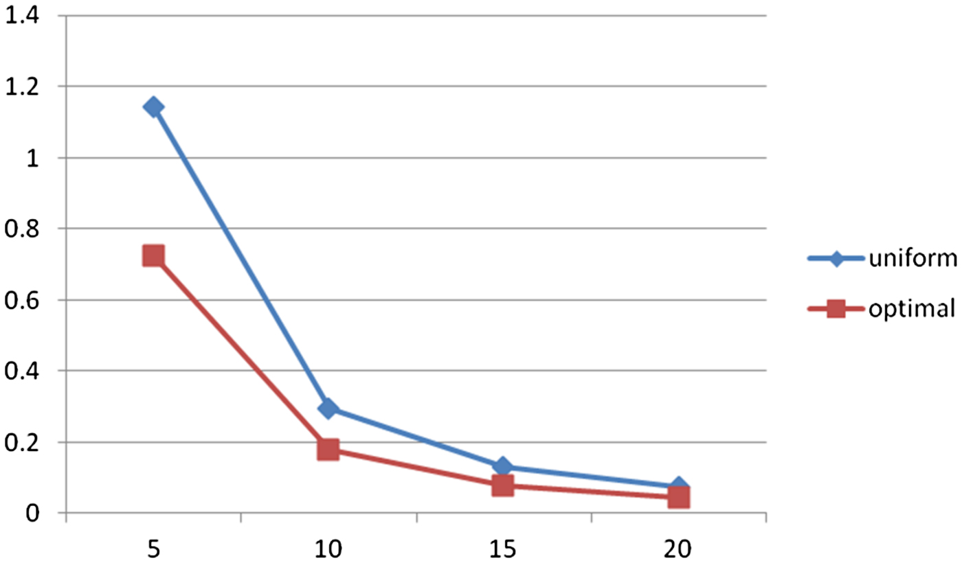
Figure 2. ∆Slxn for uniform and optimal division of the orthodrome (%).
Table 1. ∆Slxn for uniform and optimal division of the orthodrome.
Table 2. Intermediate points for n = 10 and the uniform division.
Table 3. Intermediate points for n = 10 and the optimal division.
3. SAILING ON THE PLANNED ROUTE
3.1. Course and course over the ground
The most important thing when sailing on the planned route in manual steering is to follow the calculated Cglxi whereas the course set and stabilised by an autopilot is the course through the water. Fortunately COG can be obtained from a Global Positioning System (GPS) receiver, therefore COG must be carefully observed and the course set on an autopilot must be accordingly corrected to obtain COG equal to the required Cglxi for each subloxodrome.
3.2. Return to the required route
If due to set and drift our current position is off the route (even if Section 3.1 is applied), then a new corrected Cglxi should be calculated to the nearest intermediate point. This additional loss of distance can be calculated from Equation (12) (Figure 3)
 $$\Delta {\rm s} = \displaystyle{{{\rm s}_1 + {\rm s}_2} \over {{\rm l}_1 + {\rm l}_2}} - 1 = \displaystyle{{\rm k} \over {{\rm \cos \alpha}}} + \sqrt {{(1 - {\rm k})}^2 + {({\rm k}\,{\rm tan}\,{\rm \alpha} )}^2} - 1$$
where
 $${\rm k} = \displaystyle{{{\rm l}_1} \over {{\rm l}_1 + {\rm l}_2}}$$

Figure 3. Return to the required route.
For example for α = 5° and k = 0·5 ∆s = 0·38%, for k = 0·75 ∆s = 1·13%, for k = 1 ∆s = 9·13% (although in the last case it would be better to steer to the next intermediate point and not to the nearest). It can be seen that this loss of distance can be many times bigger than the loss between loxodromes and orthodromes.
3.3. Orthodromic navigation
Let us assume that we can also use the set of procedures as in Section 2 during the voyage. Section 3.1 is still valid and very important. During the voyage if we enter as P1 the current position and P2 is constantly the destination point then Equation (2) gives the Cgs for the orthodrome to the destination point, even if we, for example, due to set and drift are off the route, and not to an intermediate point. We can calculate a new course for the orthodrome after each position fix and always navigate along the current orthodrome without these calculated intermediate points and without loss of ∆s and ∆Slxn.
Orthodromic navigation, although very promising, is possible only in automatic steering systems where an autopilot (course controller which stabilises the required course) is connected with a track controller (which nearly continuously fixes the position and calculates Cgs from the current position to the destination point) but such systems are very rare in marine navigation. Most common is a separate autopilot and for example a GPS receiver which sometimes can calculate the orthodromic or loxodromic course (mainly on a sphere) and this course must be manually set on an autopilot.
Let us assume that we will be steering with a manually set autopilot and we will be fixing position at ∆t intervals where ∆t is for example equal to 1, 2 or 4 hours. For ∆t = 1 h and our speed Vg = 20 kn for 20 NM the orthodrome at the maximum latitude of our exemplary voyage (−73·1°) Cge – Cgs = 1·1°. Let us assume that, to be very accurate, we will be changing our course in 0·1° steps, therefore our course should be changed 11 times in 1 hour to obtain 56 cm (the difference between the loxodromic and the orthodromic distance). On the other hand if we steer for 1 hour on the constant Cgs course we will be off the route by 0·19 NM. This deviation is given by equation
 $${\rm \Delta} {\rm s}_{{\rm dev}}{\rm =} \left( {{\rm C}_{{\rm glx}} \, \ndash \, {\rm C}_{{\rm gs}}} \right){\rm V}_{\rm g}{\rm \Delta t}$$
Table 4 gives these deviations for different latitudes and different Cgs for Vg∆t = 20 NM (for example ∆t = 1 hour at Vg = 20 kn). These deviations increase very quickly with longer Vg∆t as Table 5 shows (Vg∆t = 80 NM e. g. ∆t = 4 hours at Vg = 20 kn).
Table 4. ∆sdev [NM] for Vg∆t = 20 NM.
Table 5. ∆sdev [NM] for Vg∆t = 80 NM.
The solution is to steer the loxodromic course Cglx to the locally predicted position after ∆t on the orthodrome from the current position to the destination point, that is
 $${\rm \varphi} _{{\rm \Delta t}}, {\rm \lambda} _{{\rm \Delta t}} = {\rm DGP} \left( {{\rm \varphi} _{\rm c}, {\rm \lambda} _{\rm c}, {\rm V}_{\rm g}{\rm \Delta t,}\, {\rm C}_{{\rm gs}}} \right)$$
 $${\rm C}_{{\rm glx}} = {\rm LX} \left( {{\rm \varphi} _{\rm c}, {\rm \lambda} _{\rm c}, {\rm \varphi} _{{\rm \Delta t}}, {\rm \lambda} _{{\rm \Delta t}}} \right)$$
where: ϕc, λc is the current position. Such a combination of the orthodrome and short loxodromes allows orthodromic navigation in manual steering without ∆sdev and ∆s losses and quite negligible ∆Slx. For example, for 20 NM loxodromes, the maximal ∆Slx = 1·66 m and for 80 NM loxodromes, the maximal ∆Slx = ≈ 107 m - for maximal latitude 80° (Tables 6 and 7).
Table 6. ∆Slx [m] for Vg∆t = 20 NM.
Table 7. ∆Slx [m] for Vg∆t = 80 NM.
4. CONCLUSIONS
The presented procedures are quite general and universal. They can be used for any geodetic solutions and required accuracy, on any reference ellipsoid. For orthodromic navigation they can be used as well during route planning with additional optimally divided orthodromes as during sailing on the planned route with locally predicted short loxodromes.
The proposed locally predicted short loxodromes – calculated in real time during sailing at position fix intervals – also allow orthodromic navigation in manual steering without intermediate points and losses of returning to these points, without deviations caused by constant orthodromic courses and quite negligible differences in distances between loxodromes and orthodromes. In fact a dozen or so constant planned loxodromes are replaced by a few hundred short loxodromes - locally adopted to set and drift - on the orthodrome from the current position to the destination point.
It is worth mentioning that although analysis has been done on an ellipsoid, nothing prevents using the results - optimal division and locally predicted short loxodromes - in calculations even on a sphere.


