


1. INTRODUCTION
High precision and continuous geo-referencing information including position, velocity and attitude are frequently obtained by Inertial Navigation System/Global Positioning System (INS/GPS) integration that overcomes each individual system's drawbacks and are more and more used in the airborne direct geo-referencing area (Farrell and Barth, Reference Farrell and Barth1999; Bradford and James, Reference Bradford and James1996; Farrell et al., Reference Farrell, Givargis and Barth2000; Toth, Reference Toth2002). In addition to the position error, velocity error, attitude error and inertial sensor error, lever arm error between the GPS antenna centre and inertial measurement unit (IMU) sensing centre is an important error source in INS/GPS integration. Lever arm error can seriously decay position, velocity and attitude precision of INS/GPS (Xiufeng and Jianye, Reference Xiufeng and Jianye2002; Seo et al., Reference Seo, Lee, Lee and Park2006). This cannot always be measured directly under the condition that the IMU is placed inside the airplane and the GPS antenna is mounted on the airplane roof. The lever arm error together with navigation errors and inertial sensor errors are usually estimated by an Extended Kalman Filter (EKF) in the integration of INS/GPS (Geng et al., Reference Geng, Deurloo and Bastos2010; Hong et al., Reference Hong, Lee, Chun, Kwon and Speyer2006; Hong et al., Reference Hong, Lee, Rios and Speyer2002; Fang and Gong, Reference Fang and Gong2010; Stakkeland et al., Reference Stakkeland, Prytz, Booij and Pedersen2007).
The observability analysis of error states is necessary in designing the filter for the case that the unobservable error states cannot be estimated accurately. The error states in the filter should be able to become observable after a set of available measurements. Typically, the observability of error states is relatively easily analysed during the period of ground alignment. Here the INS is a time-invariant system, the analytical observability result can be found in Bar-Itzhack and Berman (Reference Bar-Itzhack and Berman1988) and Jiang and Lin (Reference Jiang and Lin1992). According to the observability results of ground alignment, multi-position alignment was adopted to improve observability of misalignment angles in ground alignment (Lee et al., Reference Lee, Park and Park1993; Chung et al., Reference Chung, Lee, Park and Park1996). While the INS is a time-varying system during in-flight alignment (IFA) of INS or INS/GPS integration, the analytical observability for time-varying systems is rather complicated.
The observability of error states in a time-varying system such as INS IFA or INS/GPS integration has been widely investigated by previous scholars. Control theoretical methodologies were adopted in most of these works. The INS was approximated as a linear constant model in a short time interval, by testing the rank of stripped observability matrix (SOM), which avoided the complexity of the observability matrix for a time-varying system and the observability of error states in a time-varying system were obtained (Goshen-Meskin and Bar-Itzhack, Reference Goshen-Meskin and Bar-Itzhack1992a). The role of translational motion in improving the observability of error states in IFA of INS were analysed (Goshen-Meskin and Bar-Itzhack, Reference Goshen-Meskin and Bar-Itzhack1992b). The local observability concept was employed to portray a system's observability in a fixed time interval, which is stronger than the global concepts in that a locally observable system is sure to be globally observable, but a globally observable system may locally be unobservable (Chen et al., Reference Chen, Jiang and Hung1990; Chen, Reference Chen1991). Null space tests of time-varying observability matrices obtained the error states' observability (Hong et al., Reference Hong, Lee, Rios and Speyer2002; Lee et al., Reference Lee, Hong, Lee, Kwon and Chun2005). The translational and angular motion's role in improving the observability of error states in alignment and integration of INS/GPS were given. The instantaneous observability method transformed the observability matrix into an observable part and an unobservable part (Rhee et al., Reference Rhee, Abdel-Hafez and Speyer2004) and a similar method was also used for the transfer alignment of INS (Zhilan et al., Reference Zhilan, Feng and Qi2006). Although by proper matrix transformation of the observability matrix, the complexity of the observability analysis can be reduced, the method cannot be applied to the universal manoeuvre in that the universal transformation matrix cannot be obtained for this mode. Meanwhile the null space test of the observability matrix for an eighteen state vector system is still very complicated, therefore, to avoid the complexity of high dimension observability matrices, time derivatives of GPS measurements were used for observability tests (Hong et al., Reference Hong, Lee, Chun, Kwon and Speyer2005), which changes the observability test on the eighteen error states to that of nine error states, errors in attitude, gyro bias, and lever arm. Compared to the analysis based upon the null space test of observability matrices, this approach reduces the complexity of the observability matrix. Additionally, a novel global observability analysis method which started from the observability definition was proposed, which can be applied to a nonlinear time-varying system (Tang et al., Reference Tang, Wu, Wu, Wu, Hu and Shen2009; Wu et al., Reference Wu, Zhang, Wu, Hu and Hu2012).
From the aforementioned analyses, it is clear that the control theoretical methods which resorted to null space tests or rank tests of observability matrices are mainly adopted to obtain the analytical observability of IFA or INS/GPS integration. For a time-varying system with high-dimensional error states vector, observability analysis is very complicated. This is because the rank test and null space test of a time-varying observability matrix is difficult. The effort to reduce the observability matrix's dimension by decoupling the error states is an important approach to making observability analysis easier. Besides, compared with the role of translational motion in improving the observability of error states in INS, excepting lever arm error, the analysis of the effect of angular motion in improving the observability of other error states for INS is not sufficient, especially with the random drift of a gyroscope and the random bias of an accelerometer. In fact, angular motion will improve the observability of the random error of the inertial sensor.
One of the main contributions of this paper is to propose the decoupled observability analysis method which decouples the observability matrix of an eighteen-dimensional state vector to several groups of six dimensional states, which make the observability analysis of error states easier. The other contribution of this paper is that the relationships between airplane motions and the observability of error states in INS/GPS integration are given, and especially the role of the angular motion in improving the lever arm error and the random error of the inertial sensor have been sufficiently analysed. Also the simulation and flying tests were performed, which validated the observability analysis results.
The rest of the paper is organized as follows. Section 2 briefly introduces the error model of the INS/GPS Integration system. Section 3 presents the decoupled observability analyses method. Section 4 presents the results of the error state observability analyses. The simulation analyses are reported in Section 5 and the experimental system and flying test are presented in Section 6. Conclusions are drawn in Section 7.
2. INS/GPS INTEGRATION ERROR MODEL
This section presents the error propagation model of INS and the measurement model of the integration of INS/GPS. The estimation of position error, velocity error, attitude error, gyroscope drift, accelerometer bias and lever arm error are considered in the error propagation equations. The linear perturbation equations for the Earth-centred Earth-fixed (ECEF) frame is
 $$\left[ {\matrix{ {{\bi \delta \dot P}} \cr {{\bi \delta \dot V}} \cr {{\bi \dot \gamma}} \cr {{\bi \dot \varepsilon} _{\bi g}} \cr {{\bi \dot \varepsilon} _{\bi a}} \cr {{\bi \delta \dot l}} \cr}} \right] = \left[ {\matrix{ {\bi 0} & {\bi I} & {\bi 0} & {\bi 0} & {\bi 0} & {\bi 0} \cr {\bi G} & { - {\bi 2\Omega} _{{\bi ie}}^{\bi e}} & { - {\bi C}_{\bi b}^{\bi e} {\bi F}^{\bi b}} & {\bi 0} & {{\bi C}_{\bi b}^{\bi e}} & {\bi 0} \cr {\bi 0} & {\bi 0} & { - {\bi \Omega} _{{\bi ib}}^{\bi b}} & {\bi I} & {\bi 0} & {\bi 0} \cr {\bi 0} & {\bi 0} & {\bi 0} & {\bi 0} & {\bi 0} & {\bi 0} \cr {\bi 0} & {\bi 0} & {\bi 0} & {\bi 0} & {\bi 0} & {\bi 0} \cr {\bi 0} & {\bi 0} & {\bi 0} & {\bi 0} & {\bi 0} & {\bi 0} \cr}} \right]\left[ {\matrix{ {{\bi \delta P}} \cr {{\bi \delta V}} \cr {\bi \gamma} \cr {{\bi \varepsilon} _{\bi g}} \cr {{\bi \varepsilon} _{\bi a}} \cr {{\bi \delta l}} \cr}} \right] + {\bi W}$$
where δP and δ P are the estimated position error and velocity error of INS, respectively; γ is the attitude error denoted in the b-frame; ε g and ε a are gyro constant drift and accelerometer bias denoted in the b-frame, respectively; δl is the lever arm error; I and 0 are the three dimensional identity matrix and zero matrix, respectively; G=∂ge/∂Pe is the gradient of gravity, Ω iee, Ω ibb and Fb are the skew-symmetric matrices of ω iee, ω ibb and fb, respectively, where ω iee is the earth's rotation rate denoted in the e-frame; ω ibb is the angular velocity of b-frame relative to i-frame denoted in the b-frame, which was measured by gyroscope; ω ebb is the angular velocity of b-frame relative to e-frame denoted in the b-frame; fb is the specific force measured by accelerometers. C be is the coordinate transformation matrix of b-frame with respect to e-frame. W=[w gTw aT]T is the driving noise of INS, w g and w a are the noise of gyroscopes and accelerometers.
The GPS measurement estimation error can be written as
 $${\bi \delta P}_{\bi 1} = {\bi \delta P} - {\bi C}_{\bi b}^{\bi e} {\bi L}_{_{\bi 1}} ^{\bi b} {\bi \gamma +C}_{\bi b}^{\bi e} {\bi \delta l} - {\bi v}_{\bi 1} $$
where δ P 1 is the GPS measurement estimation error. L 1b is the cross-product matrix of the initial lever arm l 1b , v 1 is the noise in the GPS measurement.
According to Equations (1) and (2), the system model and measurement model for the integration of INS/GPS is
 $$\left\{ {\matrix{ {{\bi \dot X(t)} = {\bi F(t)X(t) + W(t)}} \cr {{\bi Z(t) = H(t)X(t) + V(t)}} \cr}} \right.$$
where X=[δ PT δ VT γ Tε gTε aTδ lT]T, matrix F is the system equation, which is shown in (1). H is the measurement equation and
 $${\bi H} = [\matrix{ {\bi I} & {\bi 0} & { - {\bi C}_{\bi b}^{\bi e} {\bi L}_{_{\bi 1}} ^{\bi b}} & {\bi 0} & {\bi 0} & {{\bi C}_{\bi b}^{\bi e} ]} \cr} $$
The maximum singular value of G is in the order of 10−6. The magnitude of ω iee is in the order of 10−5, and that of fb is in the order of 10. The magnitude of δ P is in the order of 10−3, that of δ V is in the order of 10−4, and that of γ is in the order of 10−5 in a tactical IMU. The magnitude of ε a is in the order of 10−4 and that of ε g is in the order of 10−5 in a tactical IMU. According to the magnitude of each error item multiplying its coefficient in the error propagation equation imposed on the error states, the gravity gradient and the angular motion of the earth can be neglected. A simplified system matrix F denoted as follows can be used for observability analysis.
 $${\bi F} = \left[ {\matrix{ {\bi 0} & {\bi I} & {\bi 0} & {\bi 0} & {\bi 0} & {\bi 0} \cr {\bi 0} & {\bi 0} & { - {\bi C}_{\bi b}^{\bi e} {\bi F}^{\bi b}} & {\bi 0} & {{\bi C}_{\bi b}^{\bi e}} & {\bi 0} \cr {\bi 0} & {\bi 0} & { - {\bi \Omega} _{{\bi ib}}^{\bi b}} & {\bi I} & {\bi 0} & {\bi 0} \cr {\bi 0} & {\bi 0} & {\bi 0} & {\bi 0} & {\bi 0} & {\bi 0} \cr {\bi 0} & {\bi 0} & {\bi 0} & {\bi 0} & {\bi 0} & {\bi 0} \cr {\bi 0} & {\bi 0} & {\bi 0} & {\bi 0} & {\bi 0} & {\bi 0} \cr}} \right]$$
3. DECOUPLED OBSERVABILITY ANALYSIS METHOD
The previous observability analysis methods usually resorted to rank tests or null space tests of the observability matrix. For a high-dimensional system, the rank test or null space test of an observability matrix is very difficult. Here the observability matrix relating to the decoupled error states was obtained. By transforming the observability matrix of the time-invariant system, six error states are coupled together at most.
By the Piece-wise Constant System (PWCS) theory, the system is time-invariant during a short time interval. Fj and Hj are constant at j-th time interval. The observability matrix at j-th time interval can be denoted as
 $${\bi \tilde Q}_{\bi j} = \left[ {\matrix{ {{\bi H}_{\bi j}} \cr {{\bi H}_{\bi j} {\bi F}_{\bi j}} \cr {{\bi H}_{\bi j} {\bi F}_{\bi j}^2} \cr {\quad \vdots \quad} \cr {{\bi H}_{\bi j} {\bi F}_{\bi j}^{{\bi n - 1}}} \cr}} \right]$$
According to Equations (4) and (5), by row transformation, the matrix at the right part of the equal mark in Equation (6) can be obtained
 $${\bi \tilde {Q'}}_{\bi j} = \left[ {\matrix{ {\bi I} & {\bi 0} & { - {\bi C}_{\bi b}^{\bi e} {\rm (}j{\rm )}{\bi L}^{\bi b} {\rm (}j{\rm )}} & {\bi 0} & {\bi 0} & {{\bi C}_{\bi b}^{\bi e} {\rm (}j{\rm )}} \cr {\bi 0} & {\bi I} & {\bi 0} & {\bi 0} & {\bi 0} & {\bi 0} \cr {\bi 0} & {\bi 0} & { - {\bi F}^{\bi b} {\rm (}j{\rm )}} & {\bi 0} & {\bi I} & {\bi 0} \cr {\bi 0} & {\bi 0} & {{- \bi \Omega} _{{\bi eb}}^{\bi b} {\rm (}j{\rm )}} & {\bi I} & {\bi 0} & {\bi 0} \cr \noalign{{- - - - - - - - - - - - - - - - - - - - - - - - - - - -} } \cr \noalign{{ \matrix{{{\bi 0}_{_{{\bi 42 \times 18}}}}}}} \cr}} \right]$$
According to PWCS, the observability matrix of error states in INS/GPS integration during the jth time-interval and the (j+n)th time-interval is
 $${\bi \tilde Q}_s = \left[ {\matrix{ {{\bi \tilde {Q '}}_{\bi j}} \cr {{\bi \tilde {Q'}}_{{\bi j + 1}}} \cr \vdots \cr {{\bi \tilde {Q'}}_{{\bi j + n}}} \cr}} \right]$$
In Equation (7), from the perspective of row observation, the error states relative to zero sub-matrices can be decoupled from those relative to non-zero sub-matrices. For example, from the second row of observability in the matrix in Equation (7), the velocity error is decoupled from other error states completely. Similarly, from the first row, the position error δP, the attitude error γ and lever arm error δl are coupled together. The third row shows that the attitude error γ and accelerometer's bias ε a are coupled together. The fourth row shows that the attitude error γ and gyroscope's drift ε g are coupled together.
Also, from the perspective of column observation, the non-zero sub-matrices in column make those error states relative to non-zero sub-matrices in different rows couple together. For example, the non-zero sub-matrices in the third column appears in the first, third and fourth rows, which means that error states including position error δP, attitude error γ, gyroscope drift ε g, accelerometer bias ε a and lever arm error δl are coupled together. This coupling relationship means the observability matrix can be reduced to essentially fifteen dimensions.
Actually, for a tactical INS, the first row shows that the lever arm error will impose on the position error and attitude error. However, the magnitude of attitude error is too small to affect the estimation precision of lever arm error and position error. Therefore, the observability matrix in Equation (7) can be simplified as
 $${\bi \tilde {Q''}}_{\bi j} = \left[ {\matrix{ {\bi I} & {\bi 0} & {\bi 0} & {\bi 0} & {\bi 0} & {{\bi C}_{b}^{e} {\rm (}j{\rm )}} \cr {\bi 0} & {\bi I} & {\bi 0} & {\bi 0} & {\bi 0} & {\bi 0} \cr {\bi 0} & {\bi 0} & { - {\bi F}^{b} {\rm (}j{\rm )}} & {\bi 0} & {\bi I} & {\bi 0} \cr {\bi 0} & {\bi 0} & {{-\bi \Omega} _{{eb}}^{b} {\rm (}j{\rm )}} & {\bi I} & {\bi 0} & {\bi 0} \cr \noalign{{- - - - - - - - - - - - - - - - - - - - - - -} }\cr \noalign{{ \matrix{{{\bi 0}_{{42 \times 18}}}}}}} \cr \right]$$
Thus, from Equation (8), the non-zero sub-matrices in the first row of the observability matrix is completely different from that in the second to fourth rows, which means that the position error δP and lever arm error δl relative to non-zero matrices in first row are decoupled from the attitude error γ, gyroscope drift ε g and accelerometer bias ε a.
From the aforementioned analysis, the observability matrices for decoupled error states in INS/GPS integration during the jth time-interval and the (j+n)th time-interval are:
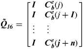
(a) The observability matrix for position error δP and lever arm error δl is
(10a) $${\bi \tilde Q}_{{\bi 16}} = \left[ {\matrix{ {\bi I} & {{\bi C}_{\bi b}^{\bi e} {\rm (}j{\rm )}} \cr {\bi I} & {{\bi C}_{\bi b}^{\bi e} {\rm (}j + {\bi I}{\rm )}} \cr \vdots & \vdots \cr {\bi I} & {{\bi C}_{\bi b}^{\bi e} {\rm (}{\bi j} + {\bi n}{\rm )}} \cr}} \right]$$
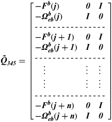
(b) The observability matrix for attitude error γ, gyroscope's drift ε g and the accelerometer bias ε a is
(10b)$${\bi \tilde Q}_{{\bi 345}} = \left[ {\matrix{ { - {\bi F}^{\bi b} {\rm (}{\bi j}{\rm )}} & {\bi 0} & {\bi I} \cr {{ - \bi \Omega} _{{\bi eb}}^{\bi b} {\rm (}{\bi j}{\rm )}} & {\bi I} & {\bi 0} \cr \noalign{{- - - - - - - - - - - - - - - - } } \cr { - {\bi F}^{\bi b} {\rm (}{\bi j} + {\bi 1}{\rm )}} & {\bi 0} & {\bi I} \cr {{ - \bi \Omega} _{{\bi eb}}^{\bi b} {\rm (}{\bi j} + {\bi 1}{\rm )}} & {\bi I} & {\bi 0} \cr \noalign{{- - - - - - - - - - - - - - - - } } \cr \vdots & \vdots & \vdots \cr \vdots & \vdots & \vdots \cr \noalign{{- - - - - - - - - - - - - - - - } } \cr{ - {\bi F}^{\bi b} {\rm (}{\bi j} + {\bi n}{\rm )}} & {\bi 0} & {\bi I} \cr {{ - \bi \Omega} _{{\bi eb}}^{\bi b} {\rm (}{\bi j} + {\bi n}{\rm )}} & {\bi I} & {\bi 0} \cr}} \right]$$
By row transformation of  ${\bi \tilde Q}_{{\bi 345}} $, the equivalent form of
  ${\bi \tilde Q}_{{\bi 345}} $ can be obtained as
 $$\left[ {\matrix{ { - {\bi F}^{\bi b} {\rm (}{\bi j}{\rm )}} & {\bi 0} & {\bi I} \cr { - {\bi F}^{\bi b} {\rm (}{\bi j} + {\bi 1}{\rm )}} & {\bi 0} & {\bi I} \cr \hskip9pt\vdots & \vdots & \vdots \cr { - {\bi F}^{\bi b} {\rm (}{\bi j} + {\bi n}{\rm )}} & {\bi 0} & {\bi I} \cr \noalign{{- - - - - - - - - - - - - - - - } } \cr {{ - \bi \Omega} _{{\bi eb}}^{\bi b} {\rm (}{\bi j}{\rm )}} & {\bi I} & {\bi 0} \cr {{\bi \Omega} _{{\bi eb}}^{\bi b} {\rm (}{\bi j} + {1}{\rm )}} & {\bi I} & {\bi 0} \cr \hskip8pt\vdots & \vdots & \vdots \cr {{ - \bi \Omega} _{{\bi eb}}^{\bi b} {\rm (}{\bi j} + {n}{\rm )}} & {\bi I} & {\bi 0} \cr}} \right]$$
Notice that the Fb(j) is the skew-symmetric matrix of specific fb in the jth time-interval, and rank (Fb(j))=2, therefore, the hypothesis that F=0 or I is a pure mathematical assumption but did not consider the real condition. Additionally, as the purpose of this paper is to investigate the observability of a time-varying system, the hypothesis that F never changed is not reasonable. For the same reason, it is also not reasonable to assume Ω ebb, keeps 0 or I at all times.
Due to Fb(j+1)−Fb(j)= $ {{\bi \dot {F^{\bi b}}}} $(j)Δt, and the similar relationship for high-order derivatives of Fb is also established, the upper part of (10c) can be transformed as
 $${\bi \tilde Q}_{{\bi 35}} = \left[ {\matrix{ {{\bi F}^{\bi b}} & {\bi 0} & {\bi I} \cr {{\bi \dot {F^{\bi b}}}} & {\bi 0} & {\bi 0} \cr \vdots & \vdots & \vdots \cr {{\bi F}^{{\bi b}^{{\bi (n)}}}} & {\bi 0} & {\bi 0} \cr}} \right]$$
 Similarly, due to Ω ebb(j+1)−Ω ebb(j)= ${\bi \dot \Omega} _{{\bi eb}}^{\bi b} $(j)Δt and the similar relationship for high-order derivatives of Ω ebb is also established. The lower part of (10c) can be transformed as
 $${\bi \tilde Q}_{{\bi 34}} = \left[ {\matrix{ {{\bi \Omega} _{{\bi eb}}^{\bi b}} & {\bi I} & {\bi 0} \cr {{\bi \dot \Omega} _{{\bi eb}}^{\bi b}} & {\bi 0} & {\bi 0} \cr \vdots & \vdots & \vdots \cr {{\bi \Omega} _{{\bi eb}}^{{\bi b}^{{\bi (n)}}}} & {\bi 0} & {\bi 0} \cr}} \right]$$
 If rank  $({\bi \tilde Q}_{{\bi 35}} ) = 6$, then, the conclusion can be made that rank
  ${\rm (}{\bi \tilde Q}_{\it{345}} ) = 9$. Similarly, if rank
  $({\bi \tilde Q}_{\it{34}} ) = 6$, then rank (
 $({\bi \tilde Q}_{\it{345}} ) = 9$). Therefore, it is reasonable to use (10d) and (10e) instead of (10b) to investigate the observability of attitude error, gyroscopes drift and accelerometer bias.
Due to 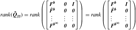 $rank({\bi \tilde Q}_{{\bi 35}} ) = rank\left( {\left[ {\matrix{ {{\bi F}^{\bi b}} & {\bi 0} & {\bi I} \cr {{\bi \dot {F^{\bi b}}}} & {\bi 0} & {\bi 0} \cr \hskip3\vdots & \vdots & \vdots \cr {{\bi F}^{{\bi b}^{{\bi (n)}}}} & {\bi 0} & {\bi 0} \cr}} \right]} \right) = rank\left( {\left[ {\matrix{ {{\bi F}^{\bi b}} & {\bi I} \cr {{\bi \dot {F^{\bi b}}}} & {\bi 0} \cr \vdots & \vdots \cr {{\bi F}^{{\bi b}^{{\bi (n)}}}} & {\bi 0} \cr}} \right]} \right)$, therefore, a six-dimensional matrix can be defined as
 $${\bi \tilde {Q'}}_{{\bi 35}} = \left[ {\matrix{ {{\bi F}^{\bi b}} & {\bi I} \cr {{\bi \dot F}^{\bi b}} & {\bi 0} \cr \vdots & \vdots \cr {{\bi F}^{{\bi b}^{{\bi (n)}}}} & {\bi 0} \cr}} \right]$$
  ${\bi \tilde Q'}_{{\bi 35}} $ can be used to investigate the observability of attitude error, gyroscope drift and accelerometer bias.
Similarly, due to 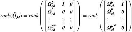 $rank({\bi \tilde Q}_{{\bi 34}} ) = rank\left( {\left[ {\matrix{ {{\bi \Omega} _{{\bi eb}}^{\bi b}} & {\bi I} & {\bi 0} \cr {{\bi \dot \Omega} _{{\bi eb}}^{\bi b}} & {\bi 0} & {\bi 0} \cr \hskip3\vdots & \vdots & \vdots \cr {{\bi \Omega} _{{\bi eb}}^{{\bi b}^{{\bi (n)}}}} & {\bi 0} & {\bi 0} \cr}} \right]} \right) = rank\left( {\left[ {\matrix{ {{\bi \Omega} _{{\bi eb}}^{\bi b}} & {\bi I} \cr {{\bi \dot \Omega} _{{\bi eb}}^{\bi b}} & {\bi 0} \cr \vdots & \vdots \cr {{\bi \Omega} _{{\bi eb}}^{{\bi b}^{{\bi (n)}}}} & {\bi 0} \cr}} \right]} \right)$, therefore, a six-dimensional matrix can be defined as
 $${\bi \tilde {Q'}}_{{\bi 34}} = \left[ {\matrix{ {{\bi \Omega} _{{\bi eb}}^{\bi b}} & {\bi I} \cr {{\bi \dot \Omega} _{{\bi eb}}^{\bi b}} & {\bi 0} \cr \vdots & \vdots \cr {{\bi \Omega} _{{\bi eb}}^{{\bi b}^{{\bi (n)}}}} & {\bi 0} \cr}} \right]$$
  ${\bi \tilde {Q'}}_{{\bi 34}} $ can be used for investigating the observability of attitude error, gyroscope drift and accelerometer bias.
Therefore, three six-dimensional observability matrices in Equations (10a), (10f) and (10g) can be used for investigating the observability of the 18-dimensional error state vector.
Remark 1: The observability matrix in the PWCS method is eighteen dimensional, while that in the decoupled observability analysis method is six dimensional. The reduction of the dimensions of the observability matrix makes the observability analysis easier.
Remark 2: It is equivalent to determine observability of attitude error γ, gyroscope drift ε g and accelerometer bias ε a by judging full column rank of  ${\bi \tilde Q'}_{{\bi 34}} $ and
  ${\bi \tilde Q'}_{{\bi 35}} $ instead of
  ${\bi \tilde Q}_{{\bi 345}} $ because if rank(
 ${\bi \tilde Q'}_{{\bi 34}} $)=6 or rank(
 ${\bi \tilde Q'}_{{\bi 35}} $)=6, then rank(
 ${\bi \tilde Q}_{{\bi 345}} $)=9, it is reasonable to decouple the observability matrix in Equation (10b) as that in Equations (10f) and (10g).
4. OBSERVABILITY PROPERTIES OF INS/GPS INTEGRATION
4.1. The observability characteristics of position error δP and lever arm error δl
The observability characteristics of position error δP and lever arm error δl can be obtained by rank test of  ${\bi \tilde Q}_{{\bi 16}} $. From Equation (10a), only angular motion can change the structure of
  ${\bi \tilde Q}_{{\bi 16}} $. Suppose that the time-interval between different segments is Δt, in that C be(j+1)−C be(j)=C be(j)(Ω ebb(j)Δt, by row transformation, the observability matrix in
  ${\bi \tilde Q}_{{\bi 16}} $ can be transformed as
 $${\bi \tilde {Q'}}_{{\bi 16}} = \left[ {\matrix{ {\bi I} & {\bi 0} \cr {\bi 0} & {{\bi \Omega} _{{\bi eb}}^{\bi b}} \cr \vdots & \vdots \cr {\bi 0} & {{\bi \Omega} _{{\bi eb}}^{{\bi b}^{{\bi (n} - {\bi 3)}}}} \cr}} \right]$$
 From Equation (11), no items exist that relate to translational motion, namely, the translational motion has no impact on improving the observability of position error δP and lever arm error δl. To make rank( ${\bi \tilde {Q\hskip.5'}}_{{\bi 16}} $)=6, there must exist two linear independent items among ω ebb,
  ${\bi \dot \omega} _{{\bi eb}}^{\bi b} $, …,
  ${\bi \omega} _{{\bi eb}}^{{\bi b}^{{\bi (n} - {\bi 3)}}} $, due to when ω ebb≠0, rank(Ω ebb)=rank(
 ${\bi \dot{\Omega}{ _{{\bi eb}}^{{\bi b}}}} $)=…=rank(
 ${\bi \Omega} _{{\bi eb}}^{{\bi b}^{{\bi (n} - {\bi 3)}}} $)=2
Theorem 1: For a tactical INS, the sufficient condition of making position error δP and lever arm error δl observable is that there exist two linear independent items among ω ebb,  ${\bi \dot \omega} _{{\bi eb}}^{\bi b} $, …,
  ${\bi \omega} _{{\bi eb}}^{{\bi b}^{{\bi (n} - {\bi 3)}}} $. The translational motion has no impact on improving the observability of position error δP and lever arm error δl.
Remark 3: Theorem 1 is easily fulfilled if the direction of  $\dot \omega _{{\bi eb}}^{\bi b} $ is different from that of ωebb, namely, two manoeuvre segments where ωebb≠0 and the directions of ωebb on two manoeuvre segments are linearly independent will make the position error δP and lever arm error δl is observable.
To investigate how manoeuvre improves certain error states' observability, we consider a two segment observability matrix in static alignment phase and angular manoeuvre phase. The observability matrix for position error δP and lever arm error δl in static alignment or straight flying with constant speed can be shown as
 $${\bi \tilde Q}_{{\bi 16}}^{\bi a} = \left[ {\matrix{ {\bi I} & {{\bi C}_{\bi b}^{\bi e}} \cr {\bi 0} & {\bi 0} \cr}} \right]$$
A simple angular manoeuvre after the static alignment phase or straight flying with constant speed phase is given as ω ebxb≠0, ω ebyb=0, ω ebzb=0. Thus, under this condition, the observability matrix is
 $${\bi \tilde Q}_{{\bi 16}}^{\bi a} = \left[ {\matrix{ 1 & 0 & 0 & 0 & 0 & 0 \cr 0 & 1 & 0 & 0 & 0 & 0 \cr 0 & 0 & 1 & 0 & 0 & 0 \cr 0 & 0 & 0 & 0 & 0 & 0 \cr 0 & 0 & 0 & 0 & 0 & { - \omega _{ebx}^b} \cr 0 & 0 & 0 & 0 & {\omega _{ebx}^b} & 0 \cr}} \right]$$
 Before angular manoeuvre, rank( ${\bi \tilde Q}_{{\bi 16}}^{\bi b} $)=3, namely, there exist three unobservable error states in the group of position error and lever arm error when the INS is in static alignment or straight flying with constant speed. While after angular manoeuvre, rank(
 ${\bi \tilde Q}_{{\bi 16}}^{\bi a} $)=5, and the first three columns in Equation (13) correspond to the position error δP, that is to say, if the airplane experiences the angular manoeuvre after the static alignment phase or straight flying with constant speed phase, the position error will be observable immediately, and two lever arm errors become observable. In Equation (13), the fourth to sixth columns respond to lever arm error δl.
  ${\bi \tilde Q}_{{\bi 16}}^{\bi a} $=(5, 6)=−ω ebxb≠0,
  ${\bi \tilde Q}_{{\bi 16}}^{\bi a} $=(6, 5)=ω ebxb≠0, which means that the angular velocity in the x direction makes the lever arm error in y and z direction observable.
Theorem 2: The position error will not be observable until the airplane experiences the angular manoeuvre. The angular velocity will make lever arm errors that are perpendicular to its direction observable.
Remark 4: There exist lever arm errors between INS and GPS. If the lever arm error is unknown, the position error of INS will be estimated with a constant lever arm error when the INS is static or straight flying with constant speed. Without angular manoeuvre, a constant lever arm error will not be eliminated from the position error. However, with a known lever arm model, the position error is observable in that the position error is the measurement. This is the difference of position error's observability between known lever arm and unknown lever arm.
4.2. The observability characteristics of attitude error γ and accelerometer bias εa
Rewrite equation  ${\bi \tilde {Q'}}_{35} $
 $${\bi \tilde {Q '}}_{{\bi 35}} = \left[ {\matrix{ {{\bi F}^{\bi b}} & {\bi I} \cr {{\bi \dot F}^{\bi b}} & {\bi 0} \cr \vdots & \vdots \cr {{\bi F}^{{\bi b}^{{\bi (n)}}}} & {\bi 0} \cr}} \right]$$
 From Equation (14), to make the attitude error γ and accelerometer bias ε a become observable, rank( ${\bi \tilde {Q'}}_{{\bi 35}} $)=6 must be satisfied, if there exist n-order time derivatives of fb, there must exist two linear independent items between
  ${\bi \dot {{f}^{\bi b}}}, \ldots, {\bi f}^{{\bi b}^{{\bi (n)}}} $, because
  $rank({\bi F}^{\bi b} ) = rank({\bi \dot {F^{\bi b}} ) = \cdots = rank({\bi F}^{{\bi b}^{{\bi (n)}}} ) = 2$.
Theorem 3: For a tactical INS, the sufficient condition of making attitude error γ and accelerometer bias ε a observable is that there exist two linear independent items among  ${\bi \dot {f^{\bi b}}}, \ldots, {\bi f}^{{\bi b}^{{\bi (n)}}} $.
Remark 5: Theorem 3 is easily fulfilled if  ${\bi \dot {f^{\bi b}}} \ne {\bi 0}$,
 ${\bi \ddot {f^{\bi b}}} \ne {\bi 0}$, and the direction of
  ${\bi \ddot {f^{\bi b}}} $ is different from that of
  ${\bi \dot {f^{\bi b}}} $, namely, the direction of
  ${\bi \dot {f^{\bi b}}} $ must change twice to make the attitude error and accelerometer bias observable; an ‘s’-shape or ‘8’-shape manoeuvre can meet this requirement.
To investigate how translational manoeuvre improves certain error states' observability, we consider a two segment observability matrix in the static alignment phase and translational manoeuvre phase. The observability matrix for attitude error γ and accelerometer bias ε a in static alignment or straight flying with constant speed can be shown as
 $${\bi \tilde {Q^{\bi b}}}_{{\bi 35}} = \left[ {\matrix{ {{\bi F}^{\bi b}} & {\bi 1} \cr {\bi 0} & {\bi 0} \cr}} \right]$$
 A simple translational manoeuvre after the static alignment phase or straight flying with constant speed phase is given as  $\dot {f_x^b} \ne 0$,
  $\dot {f_y^b} = 0$,
  $\dot {f_z^b} = 0$. Thus, under this condition, the observability matrix for this manoeuvre is
 $${\bi \tilde Q}_{{\bi 35}}^{\bi a} = \left[ {\matrix{ 0 & { - f_z^b} & {\,f_y^b} & 1 & 0 & 0 \cr {\,f_z^b} & 0 & { - f_x^b} & 0 & 1 & 0 \cr { - f_y^b} & {\,f_x^b} & 0 & 0 & 0 & 1 \cr 0 & 0 & 0 & 0 & 0 & 0 \cr 0 & 0 & { - \dot {f_x^b}} & 0 & 0 & 0 \cr 0 & {\dot {f_x^b}} & 0 & 0 & 0 & 0 \cr}} \right]$$
 Before a translational manoeuvre, rank( ${\bi \tilde Q}_{{\bi 35}}^{\bi b} $)=3, namely, there exist three unobservable error states in the group of attitude error γ and accelerometer bias ε a when the INS is in static alignment or straight flying with constant speed. While after a translational acceleration manoeuvre, rank(
 ${\bi \tilde Q}_{{\bi 35}}^{\bi a} $)=5, that is to say, if the airplane changes its acceleration after a static alignment phase or straight flying with constant speed phase, two observable error states among attitude error γ and accelerometers bias ε a will be increased. In Equation (13), the second and third columns respond to attitude error γ.
 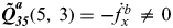 ${\bi \tilde Q}_{{\bi 35}}^{\bi a} (5,\,3) = - \dot {f_x^b} \ne 0$,
 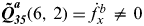 ${\bi \tilde Q}_{{\bi 35}}^{\bi a} (6,\,2) = \dot {f_x^b} \ne 0$, which means that the changing translational acceleration in the x direction makes the attitude error in y and z directions observable. Furthermore, from the observation of the first three rows of
  ${\bi \tilde Q}_{{\bi 35}}^{\bi a} $, the observable attitude in y and z directions will make the accelerometer bias in the x direction observable; for that the attitude error in x direction is unobservable and the accelerometer bias in y and z directions will be unobservable.
Theorem 4: The changing translational acceleration makes the attitude error that is perpendicular to its direction observable, and the accelerometer bias that is parallel to its direction will be observable, too. Constant acceleration has no impact on improving the attitude error.
4.3. The observability characteristics of attitude error γ and gyroscope drift εg
Rewrite equation  ${\bi \tilde {Q\hskip1'}}_{{\bi 34}} $
 $${\bi \tilde {Q '}}_{{\bi 34}} = \left[ {\matrix{ {{\bi \Omega} _{{\bi eb}}^{\bi b}} & {\bi I} \cr {{\bi \dot {\Omega_{{\bi eb}}^{\bi b}}} } & {\bi 0} \cr \vdots & \vdots \cr {{\bi \Omega} _{{\bi eb}}^{{\bi b}^{{\bi (n)}}}} & {\bi 0} \cr}} \right]$$
 Similar to Sub-Section 4.2, suppose there exist n-order time derivatives of Ω ebb, the sufficient condition of making attitude error γ and gyroscope drift ε g observable is that there exist two linear independent items among  ${\bi \dot \Omega} _{{\bi eb}}^{\bi b}, \ldots, {\bi \Omega} _{{\bi eb}}^{{\bi b}^{{\bi (n)}}} $, because
  $rank({\bi \Omega} _{{\bi eb}}^{\bi b} ) = rank({\bi \dot {\Omega _{{\bi eb}}^{\bi b}}} ) = \cdots = rank({\bi \Omega} _{{\bi eb}}^{{\bi b}^{{\bi (n)}}} ) = 2$.
Theorem 5: For a tactical INS, the sufficient condition of making attitude error γ and gyroscope drift ε g observable is that there exist two linear independent items among  ${\bi \dot {\Omega_{{\bi eb}}^{\bi b}}} , \ldots, {\bi \Omega} _{{\bi eb}}^{{\bi b}^{{\bi (n)}}} $.
Remark 6: Theorem 5 is easily fulfilled if  ${\bi \dot {\Omega^{\bi b}}}\hskip-4 _{{\bi eb}} \ne {\bi 0}{\rm,} \,{\rm} {\bi \ddot {\Omega_{{\bi eb}}^{\bi b}}} \ne {\bi 0}$, and the direction of
  ${\bi \ddot {\Omega _{{\bi eb}}^{\bi b}}} $ is different from that of
  ${\bi \dot {\Omega_{{\bi eb}}^{\bi b}}} $, namely, the direction of
  ${\bi \dot {\Omega _{{\bi eb}}^{\bi b}}} $ must change twice to make the attitude error γ and gyroscope drift ε g observable, constant angular velocity has no impact on improving the observability of attitude error and gyroscope drift.
The observability matrix for attitude error γ and accelerometer bias ε a in static alignment or straight flying with constant speed can be shown as
 $${\bi \tilde Q}_{{\bi 34}}^{\bi b} = \left[ {\matrix{ {{\bi \Omega} _{{\bi eb}}^{\bi b}} & {\bi I} \cr {\bi 0} & {\bi 0} \cr}} \right]$$
 A simple translational manoeuvre after the static alignment phase or straight flying with constant speed phase is given as  $\dot \omega _{ebx}^b \ne 0, - \dot \omega _{eby}^b = 0,\,\dot \omega _{ebz}^b = 0$. The observability matrix for this manoeuvre is
 $${\bi \tilde Q}_{{\bi 34}}^{\bi a} = \left[ {\matrix{ 0 & { - \omega _{ebz}^b} & {\omega _{eby}^b} & 1 & 0 & 0 \cr {\omega _{ebz}^b} & 0 & { - \omega _{ebx}^b} & 0 & 1 & 0 \cr { - \omega _{eby}^b} & {\omega _{ebx}^b} & 0 & 0 & 0 & 1 \cr 0 & 0 & 0 & 0 & 0 & 0 \cr 0 & 0 & { - \dot \omega _{ebx}^b} & 0 & 0 & 0 \cr 0 & { - \dot \omega _{ebx}^b} & 0 & 0 & 0 & 0 \cr}} \right]$$
 Before the angular manoeuvre, rank( ${\bi \tilde Q}_{{\bi 34}}^{\bi b} $)=3, namely, there exist three unobservable error states in the group of attitude error γ and gyroscope drift ε g when the INS is in static alignment or straight flying with constant speed. While after the angular acceleration manoeuvre, rank(
 ${\bi \tilde Q}_{{\bi 34}}^{\bi a} $)=5, that is to say, if the airplane changes its angular acceleration after the static alignment phase or straight flying with constant speed phase, two observable error states among attitude error γ and gyroscope drift ε g will be increased. In Equation (19), the second and third columns correspond to attitude error γ.
  ${\bi \tilde Q}_{{34}}^{a} (5,\,3) = - \dot \omega _{ebx}^b \ne 0$,
  ${\bi \tilde Q}_{{34}}^{a} (6,\,2) = - \dot \omega _{ebx}^b \ne 0$, which means that the changing angular acceleration in the x direction makes the attitude error in y and z directions observable. Furthermore, from the observation of the first three rows of
  ${\bi \tilde Q}_{{\bi 34}}^{\bi a} $, the observable attitude in y and z directions will make the gyroscope drift in the x direction observable; for that the attitude error in the x direction is unobservable, the gyroscopes drift in the y and z directions will be unobservable.
Theorem 6: The changing angular acceleration makes the attitude error that is perpendicular to its direction observable, and the gyroscope drift that is parallel to its direction will be observable, too. Constant angular velocity has no impact on improving the attitude error and gyroscope drift.
Theorem 7: Under changing angular acceleration or changing translational acceleration, the attitude error will be observable, thus, by  ${\bi \tilde Q}_{{\bi 34}5} $ in Equation (10b), the accelerometer bias and gyroscope drift are observable.
5. SIMULATION RESULTS
To investigate the observability of error states, covariance analysis is employed in this section, and a flying trail which included different manoeuvre styles was simulated.
In the simulation, INS output data is at 100 Hz and a DGPS position was used for measurement. The integration of INS/GPS was executed with an EKF. The signal noises of both GPS and the IMU were assumed to be Gaussian white. The standard deviation (STD) of the noise in the GPS position measurement denoted in the tangential frame was [0·05, 0·05, 0·05] in metres. Bias and the STD of the accelerometer noise were [0·0001; 0·0001; 0·0001] and 0·0005 in m/s2, respectively. Drift and the STD of gyro drift noise were [0·01; 0·01; 0·01] and 0·02 in °/h, respectively. The lever arm between GPS antenna and IMU are 3, -2, 3 metres in right, forward and upward directions, respectively.
The flying trail of the airplane in the simulation is given in Figure 1. The initial yaw, pitch and roll of the aircraft is 0,0,0 in degrees, respectively, and the initial latitude, longitude, and height are 39·5°, 116·5°, 100 metres, respectively. The aircraft remained static for 100 seconds; after that, it accelerates with constant acceleration of 3 m/s2 for 40 seconds; then the aircraft takes off with pitch changing with time for 100 seconds. The aircraft flies to the specified altitude of 6000 metres, it makes roll manoeuvres, then it flies with constant velocity. The aircraft's attitude, attitude rate and its specific force are shown in Figures 2 to 4.

Figure 1. Flying trail.
Figure 2. Attitude rate.
Figure 3. Specific force.
Figure 4. Attitude estimation error.
Figure 5. Lever arm estimation.
From Figure 4, it can be seen that the estimation of attitude error did not converge in the first 100 seconds, at this time period of the simulation, the airplane was static, which confirms that the attitude error is not observable when the INS is static. The estimation of yaw error and pitch error begin to converge after 100 s, while the roll error does not converge until after 140 s. From Figure 3, the specific force in the forward direction changing with time from 100 s, according to Theorems 3 and 4, which will help improve the yaw and pitch estimation. Similarly, the specific force in the upward direction changes from 140 s, which will help improve the estimation of pitch and roll. Therefore, the estimation of attitude error in Figure 4 proved Theorems 3 and 4 well.
In Figure 5, the red dashed line is the true lever arm and the blue solid line is the lever arm estimation value. It is shown that the lever arm estimation was not improved before 140 s. From Figure 2, at this time period of the simulation, the airplane did not experience any angular manoeuvre. The lever arm estimation began to converge in the forward and upward directions from 140 s while that in the right direction did not converge until after 240 s. According to Theorems 1 and 2, the changing angular velocity will improve the observability of lever arm error. From Figure 2, the angular velocity changes in the right direction from 140 s to 240 s, while it changes in the forward direction from 240 s to 300 s, which accounts for the lever arm estimation results. Therefore, the estimation of lever arm in Figure 5 proved Theorems 1 and 2 well.
From Figure 6, it is shown that the estimation of accelerometer bias in the right and forward directions did not converge in the first 100 s, while that in upward direction converged. At this time period of the simulation, the airplane was static, which shows that the accelerometer bias in the upward direction is observable. This phenomenon is because the airplane's upward direction is parallel to the gravity direction, therefore, the specific force in right and forward directions will be zero, the observability matrix  ${\bi \tilde {Q_{{\bi 35}}^{\bi b}}} $ in Equation (16) will become
 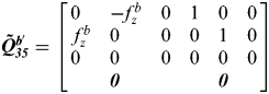 ${\bi \tilde {Q_{{\bi 35}}^{{b'}}}} = \left[ {\matrix{ 0 & { - f_z^b} & 0 & 1 & 0 & 0 \cr {\,f_z^b} & 0 & 0 & 0 & 1 & 0 \cr 0 & 0 & 0 & 0 & 0 & 0 \cr {} & {\bi 0} & {} & {} & {\bi 0} & {} \cr}} \right]$. Thus, the accelerometer bias in the upward direction which corresponds to
  ${\bi \tilde Q}_{{\bi 35}}^{b'} (3,6)$ is decoupled from the attitude error and accelerometer bias in the right and forward directions. The accelerometer bias in the forward direction came to converge from 100 s, while that in the right direction converges from 140 s. From Figure 3, the specific force in the forward direction changed from 100 s, according to Theorem 4, which will help improve the estimation of accelerometer bias in the forward direction. Although the specific force in the right direction did not change until after 240 s, from Figure 4, yaw error starts to converge from 100 s while roll error converges from140 s. According to Theorem 7, the observable yaw and roll error will help improve the accelerometer bias observability in the right direction. In this simulation, the observable roll error is more helpful to estimate the right accelerometer bias than the yaw error. The accelerometer bias estimation in Figure 5 proved Theorems 3, 4 and 7 well.
Figure 6. STD of accelerometers constant bias.
From Figure 7, it is shown that the estimation of gyroscope drift in the upward direction started to converge from 300 s. In Figure 2, the yaw rate changes from 300 s, according to Theorems 5 and 6, the angular velocity in the upward direction will help improve the estimation of gyroscope drift in the upward direction. While the estimation of gyroscope drift in the right direction started to converge from 100 s, the gyroscope drift coupling with attitude error perpendicular to its direction, in Figure 4, it is seen that the yaw and roll estimation started to converge from 100 s and 140 s, respectively. According to Theorem 7, the observable attitude error will help improve the gyroscope drift estimation, which accounts for why the gyroscope drift in the right direction started to converge from 100 s. Similarly, the gyroscope drift in the forward direction starts to converge from 100 s, and the yaw and pitch start to converge from 100 s, which confirms Theorems 5, 6 and 7.
Figure 7. STD of gyroscope drift.
6. MEASUREMENT SYSTEM AND FLYING TEST RESULTS
The theoretical deduction and simulation described in the previous sections shows that manoeuvring plays an important role in improving the observability of error states. In this section, flying tests were carried out to verify the theoretical deduction and simulation.
The integration of INS/GPS can provide precise position, velocity, and attitude information to an airborne remote sensing load such as synthetic aperture radar (SAR) and charge-coupled device (CCD) array cameras for motion compensation. During June and July 2011, flying tasks were executed to investigate the area where the earthquake occurred in Wen Chuan, Sichuan province, China in 2008. The measurement system used in the experiments consists of a “Citation-II” airplane, laser gyro IMU, POS computer system (PCS), and NovAtel DL-V3 GPS receiver. Position measurement was obtained by the NovAtel dual-frequency carrier-phase differential GPS receiver with a position precision of less than 5 cm. Angular rate was measured by laser gyroscopes with random drift of 0·01°/h, the acceleration was measured by quartz flexible accelerometers with random bias of less than 50 μg. To obtain the differential GPS data, a NovAtel receiver base was placed in the centre of the mapping area. The IMU data was measured at 100 Hz and the real-time GPS was measured at 1 Hz, while the off-line differential GPS was acquired at 20 Hz. The measurement system is shown in Figure 8.
Figure 8. Measurement system.
The IMU was mounted inside the airplane while the GPS was placed on the roof of the airplane, the true lever arm between GPS antenna centre and IMU sensing centre was -0·0113, 0·7048, 1·3890 in metres in right, forward and upward directions, respectively, and the lever arm was measured by a laser total station instrument made by the Leica company with measurement precision of less than 1 mm.
In the experiment on 28 June 2011, the airplane remained static for 900 s to complete static initial alignment, then the airplane took off. Before entering the mapping area, the airplane made an “8” shape manoeuvre to enhance the observability of system, then flew straight and level to fulfil remote sensing/mapping. The track of the airplane in the first 3600 s is shown in Figure 9.
Figure 9. Flying track in first 3600s.
The attitude and its rate are shown in Figures 10 and 11.
Figure 10. Attitude.
Figure 11 Attitude rate.
The lever arm estimation error is shown in Figure 12, the initial value of lever arm was set as 1, 1, 1 in metres in right, forward, and upward directions, respectively.
Figure 12. Lever arm estimation.
From Figure 12 and Table 1, it can be seen that the lever arm estimation started to converge from 1000 s to 1350 s when the airplane was taking off; during this time-span, the attitude rate changed sharply and the lever arm estimation precision came to less than 10 cm. Then, the lever arm estimation precision improved further from 1650 s to 1900 s. During this time-span, the airplane took the ‘8’ shape manoeuvre, which has been shown to improve the estimation of lever arm effectively. The estimation precision of lever arm came to be less than 3 cm. The estimation of lever arm proved Theorems 1 and 2.
Table 1. Estimation of lever arm in flying experiment at 3600 s.

From Figure 14, it is shown that the estimation of attitude error converges in the same way as in the simulation. The estimation of attitude error did not converge from 1000 s, since the airplane only started to take off after the first 1000 s of static alignment, the attitude rate as well as specific force (Figure 13) changed quickly in three directions, which makes the estimation of attitude converge quickly. Therefore, the observability of attitude error in Figure 14 proved Theorems 3 and 4 well.
Figure 13. Specific force.
Figure 14. STD of attitude error.
From Figure 15, it can be seen that the estimation of accelerometer bias converges in the same way as in the simulation. The estimation of accelerometer bias in right and forward directions started to converge from 1000 s, while that in the upward direction converged from the static stage. The accelerometers bias estimation in Figure 15 proved Theorems 3, 4 and 7 well.
Figure 15. STD of accelerometer bias error.
From Figure 16, it can be seen that the estimation of gyroscope drift converges in the same manner as in the simulation. The estimation of gyroscope drift in the right and forward directions started to converge from 1000 s, while that in the upward direction converged slowly, which accounts for the fact that the observability of gyroscope drift in the upward direction is more affected by angular rotation in the upward direction. The gyroscope drift estimation in Figure 16 proved Theorems 5, 6 and 7 well.
Figure 16. STD of gyroscope drift
7. CONCLUSIONS
The decoupled observability analysis method in INS/GPS integration was proposed in this paper, which changes the observability test on the 18 error states to that on six error states, which makes the observability analysis easier. The observability of error states include position error, velocity error, attitude error, gyroscope drift, accelerometer bias and lever arm error and are analysed by the decoupled observability method. Compared to previous studies, the conclusion that the attitude error as well as gyroscope drift and accelerometer bias were not only affected by linear motion but also affected by angular motion was drawn in this paper. The simulation and flying test proved the analysis result.
ACKNOWLEDGEMENTS
The authors would like to thank Chinese Academy of Sciences for assistance with the flight platform and SAR joint flying. The authors also would like to thank Beijing Institute of Surveying and Mapping for their precise lever arm measurement using total laser station.


