


Introduction
Law Dome is a small (200 km diameter) ice cap situated at the edge of the main East Antarctic ice sheet but with independent ice flow (Reference Pfitzner,Pfitzner, 1980). The Dome projects into the predominantly easterly atmospheric circulation produced by low-pressure systems centred around 65 °S (Reference Bromwich,Bromwich, 1988), and the disturbance it produces in the flow results in exceptionally high accumulation: up to 1.2 m ice equivalent on the eastern side of the Dome. The Dome Summit South (DSS) drilling site is 4.6 km south-southwest of the highest point on the dome (A001). A location map is shown in Figure 1 and a “wire mesh” view of the bedrock topography in Figure 2.

Fig. 1. Location map of DSS on Law Dome showing glaciological data. Elevation contours are light lines. Accumulation contours in kg m−2 are the heavier lines. Measured ice-sheet Surface velocities are indicated by arrows of scale length. The highest point on the dome is the apex of the survey triangle nearest DSS. (Adapted from Reference Xie,, Li and Young.Xie and others (1989).)

Fig. 2. “Wire mesh” view of the bedrock and ice surface around Law Dome summit. The survey grid is 15 km × 15 km, and the bedrock is exaggerated in the vertical by five times. The surface ice velocity is zero near (just north of) the highest point on the dome, A001.
The aim of the drilling has been to produce an accurately dated ice-core environmental record, with good time resolution in the Holocene, and extending back through the Last Glacial Maximum (LGM). The site facilitates this because the high annual accumulation results in unambiguous annual ice layers which can be reliably detected by a variety of measurements and counted to produce accurate dating.
Fieldwork started in 1987 – 88 with thermal drilling to 96 m. The 270 mm diameter borehole made by the large-diameter thermal drill was cased to a depth of 82 m. In the following season an 18 m × 7 m × 5 m high corrugated-steel arch shelter was set up over the casing, and the drill winch and support equipment installed. The electro-mechanical drill was completed and tested over the next 2 years. Electromechanical drilling to a depth of 553 m was carried out in 1991 – 92, and the remainder of the drilling was completed in 1992 – 93. Silty ice containing small rock fragments was reached at a depth of 1196 m, and drilling ceased when the drill cutters were damaged on a larger, basal rock fragment which grooved the core but was not recovered. The depth of the ice has been measured by radio-echo sounding (RES) at 1220 m; however, due to the transmit pulse not being properly recorded, the uncertainty in the depth is estimated at 20 m. The amount of silty basal ice is therefore not known but is probably less than 20 m.
On-site measurements were made of electrical conductivity, peroxide concentration, crystal size and orientation, and samples were cut for oxygen isotope ratio (δ18O), deuterium excess (δ = δD − δ18O) and 10Be determination. Continuous measurements stopped at 391 m because of time constraints and the difficulty of handling brittle core. Crystal size and orientation fabrics were measured over the full depth of the core. Ice from 552 – 1190 m was extremely brittle and was left in the drilling shelter to strain relieve over the 1993 winter. The bottom 6 m of ice had no visible bubbles and was not brittle.
Drilling Site
The high accumulation and moderate ice thickness near Law Dome summit result in an extended Holocene record, the Wisconsin/Holocene transition being quite close to the bedrock. Previous work on Law Dome (Reference Morgan, and McCray.Morgan and MсCray, 1985) and recent analysis of Greenland cores (Reference Taylor,Taylor and others, 1993) suggest that flow distortions and zones of enhanced shear in the lower layers of ice sheets can produce disturbances in ice-core data records. The DSS site was selected using RES to identify areas where laminar within-ice echoes extended to the greatest depth. These echoes (which are produced by small changes in the permittivity of the ice, e.g. from differing impurity levels) are generally thought to indicate past ice-sheet surfaces. On the basis that the laminar echoes indicate relatively undisturbed ice flow, the DSS site is removed from the summit (and ice divide) because RES there shows bedrock hills up to 250 m high, and within-ice layer echoes indicate disturbed ice flow at up to one-third of the ice thickness from the bedrock (Reference Hamley,, Morgan., Thwaites and Gao.Hamley and others, 1986). DSS is 4.6 km south-southwest (bearing 195 °) from the summit in an area of relatively level bedrock (see Fig. 3).

Fig. 3. RES profile along the flowline from the DSS borehole upStream to the dome summit, A001.
The dynamics of the Law Dome ice sheet reflect the east-west accumulation gradient across the dome. On the western side, accumulation varies from 0 to 0.7 m a−1 (ice equivalent), and ice surface velocities are generally less than 10 m a−1. To the cast, however, accumulation reaches 1.4 m a−1, and at DE08, just 16 km downslope from the summit, accumulation is 1.2 m a−1, and the ice flow towards Williamson Glacier reaches 18 m a−1. DSS is on the accumulation isopleth which crosses the summit, and has a surface velocity of 2.9 m a−1 at 220 °. The RES profile shown in Figure 3 runs from DSS upstream to the dome summit at A001.
The mean annual temperature at DSS is −21.8 ° C, low enough to generally preclude melt in summer. Visible stratigraphy of the core indicates many thin glaze layers; however, these are fairly uniformly distributed and are therefore thought to be due to the action of wind on persisting surfaces rather than to radiation in the summer. Site parameters are summarised in Table 1.
Table 1. DSS site parameters

Ice-Core Dating
The high accumulation and the absence of very strong-winds at Law Dome summit (see data of Reference Allison,, Wendler and Radok.Allison and others, 1993) result in the formation and preservation of exceptionally clear annual accumulation layers. The seasonal accumulation layers are detected by fine-detail (10 – 15 points per year) δ18O, H2O2 (Reference Sigg, and NeftelSigg and Neftel 1988), trace-chemicals and electrical-conductivity (Reference Hammer,Hammer, 1980) measurements. δ18O is the principal indicator, the Other measurements being used if necessary to resolve ambiguities. This is effective because different mechanisms produce the seasonal cycle in the different parameters. Only the irregularities in snowfall and accumulation affect all parameters, but at DSS these are relatively small. The clearest indicator is the peroxide trace because its production is modulated by the regularly varying solar radiation; however, the non-automated peroxide measurements are very time-consuming, so the record is not complete. Figure 4 shows a section of fine-detail measurements. Currently, layer-counting is continuous to 399 m (AD 1304), and spot measurements of layer thickness (from fine-detail isotope and peroxide measurements) are used to constrain an ice-flow model which is used to extrapolate the dating further down. The deepest annual layers so far detected (by peroxide) are at 1080 m where the thickness is 18 mm. Ultimately it is expected that accurate dating will be obtained by layer-counting and interpolation to a depth of about 1100 m (~8000 BP).
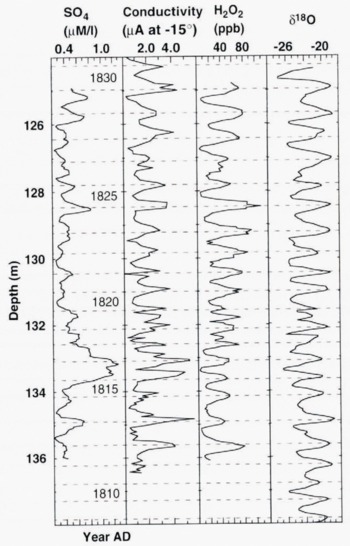
Fig. 4. Fine-detail δ peroxide, electrical conductivity and sulphate data. The Tambora (Indonesia) volcanic eruption of 1815 is seen as the small enhancement in the conductivity profile and the much larger increase in sulphate concentration around 133 m depth. The data around 132 m are one of the more ambiguous sections of the record.
In the 683 years of continuous isotope data there are about 15 places where the annual δ18O cycles are ambiguous. Cross-checking with peroxide and electrical-conductivity data resolves about half of these, leaving a dating uncertainty of 1%. An absolute check on the dating is obtained by identifying fallout from well-dated volcanic eruptions. The eruption dates of Agung (1963), Krakatau (1883) and Tambora (1815) all agree with the dating front layer-counting, although the exact position of the Krakatau peak is not clear, because the sulphate-poor eruption is almost masked by background sea-salt sulphate. A large sulphate peak found at a depth corresponding to the austral summer 1458 – 59 is assumed to be due to the eruption of Kuwae,Vanuatu. The size of this eruption, which Reference Monzier,, Robin and EissenMonzier and others (1994) suggest is one of the largest in the last 10 000 years, has only recently been recognised because the caldera is submerged. It is the largest peak in the DSS record, with nearly 1.5 times as much sulphate as the next largest, Gunung Tambora in 1815. Monzier and others used radiocarbon dating to place the eruption of Kuwae between 1420 and 1450; however, Reference Pang,Pang (1993) has used historical data to obtain a precise date of 1453. Data from several Antarctic and Greenland cores (Reference Langway,, Osada, Clausen, Hammer and ShojiLangway and others, 1995) put the date between 1450 and 1464, with the best-dated cores giving 1457 and 1459. Both the G15 (Mizuo) core (Reference Moore,, Narita and MaenoMoore and others, 1991) and the GISP2 core, Greenland (Reference Zielinski,Zielinski and others, 1994), give the date of Kuwae as 1459 – 60, making Pang’s earlier date difficult to accommodate. Current DSS layer-counting dates the onset of fallout to late 1458, which implies an eruption in 1457, since aerosols injected in mid- or low latitudes generally take 6 – 12 months to diffuse to the polar regions (Reference Handler,Handler, 1989) and entry into the polar Stratosphere usually occurs in spring after the breakdown of the polar vortex (Reference Deshler,, Adriani, Gobbi, Hofmann, Donfrancesco and Johnson.Deshler and others, 1992). A generous interpretation of the accumulation layers is required to find an extra 4 years in the DSS record between the fixed point at 1815 and 1457. Confirmation of the date of this eruption by an alternative precision method (e.g. tree-ring counting) is required. Ice-core sulphate levels from volcanic fallout are shown in Figure 5.

Fig. 5. Non-sea-salt sulphate concentrations at depths corresponding to the dates of known explosive volcanic eruptions or where conductivity measurements indicated high acidity levels. The sea-salt component is removed by subtracting 0.052 times the chloride concentration.
Dating for the whole core has been calculated using the Reference Dansgaard, and JohnsenDansgaard and Johnsen (1969) modification of the Nye time-scale to extrapolate the dating obtained by layer-counting. This model assumes the vertical strain rate is uniform from the surface down to a specific depth (break point) and then decreases linearly to zero at the bed. The equations strictly apply only at an ice divide, or at a location where the ice thickness and accumulation are constant upstream to the ice divide. DSS is only four ice thicknesses from the summit, and the thickness and accumulation vary little in this distance, so the error introduced is small.
For the DSS core, as noted earlier, the total ice-sheet thickness is not precisely known at this stage. For this reason, the equations of Reference Dansgaard, and JohnsenDansgaard and Johnsen (1969) have been recast in terms of ice depth rather than height above the base of the ice sheet. This gives equations which are independent of the ice-sheet thickness in the region above the break point in ice flow (i.e. the point at which the modelled vertical strain rate starts to decrease). Layer thickness and age relationships then simplify to:
-
1. From the surface down to the break point Layer thickness,
 Layer age,
-
2. At the break point (depth, dbreak = 2D − T)
-
3. Below the break point
 Layer age,


where d is the ice-equivalent depth; λs and D are the intercepts of the above-break linear region with a thickness and depth axes, respectively; the parameter a is the ice-equivalent annual accumulation λs/(1 year); and T is the ice-equivalent total ice thickness.

Fig. 6. DSS measured annual layer thickness (in ice equivalent) and the model data. The top 391 m of continuous data have been smoothed with a Gaussian filter of RMS width 3 years. The data points below 391 m are obtained from typically 6 years’ data, and the indicated errors are of 1 σ amplitude. The broken line shows the best-fit model which is used for dating.
The layer-thickness data were fitted to this model using a non-linear least-squares algorithm for the parameters a, D and T. The thickness data and the fit are plotted in Figure 6, and the values derived are:
a = 0.6781 ± 0.0006 m year−1
D = 1054.4 ± 0.6 m
T = 1178 ± 2 m
The ice-equivalent quantities have been computed from an exponential firn-density model (Reference Paterson,Paterson, 1994, p. 14) based on measured densities. Dating of pre-Holocene ice is problematic. The effect of variations in the accumulation rate, ice-sheet size and flow properties of the basal ice is difficult to estimate. The approach used to estimate ages prior to the Holocene has been to apply the same model and parameters with an adjusted accumulation rate of 40% of the Holocene value. Using this method, the computed age at the LGM is ~13 800 years. Based on the observed sensitivity of the model to errors in the measured layer thicknesses, and uncertainties in Wisconsin accumulation, the estimated uncertainty in this age is approximately 20%. Modelled ages improve in accuracy at shallower depths, with estimated un-certainties of ~10% at 7000 years and ~5% at 4000 years. The dating obtained is shown with the isotope profile in Figure 7.

Fig. 7. Oxygen-isotope ratio profile for DSS ice core. The top 391 m is from smoothed fine-detail (~10 per year) measurements. The 391 – 1000 m section comprises 0.5 m contiguous samples. The transition, LGM and Wisconsinan, is from spot samples, and the basal ice is sections with measurements at 10 mm intervals.
Isotope/Climate Records
The complete DSS δ18O profile is shown in Figure 7. The data are smoothed in the depth domain by differing amounts at different depths to compensate for changes in the sampling interval and layer thickness.
The 7.0‰ shift in δ18O between the LGM and the Holocene is about the same as that for the coastal Law Dome cores BHC-1 and BHC-2 (Reference Morgan, and McCray.Morgan and MсCray, 1985); however, the transition is sharper in DSS because all the ice originates from the same site. In BHC-1 and BHC-2 the surface ice is deposited near the drilling sites at low elevations, while the deeper, older ice originated upstream from near the summit of the ice sheet. The 3.0‰ change in surface δ18O values between the edge and the summit of Law Dome therefore results in a curved Holocene δ18O profile for the coastal cores which blends smoothly into the transition to the LGM. This makes it difficult to determine accurately the size of the Holocene/LGM change because correcting the profiles for deposition site is hindered by the lack of an accurate time-scale for the coastal cores. The 7.0‰ Holocene/LGM δ18O shift at DSS is larger than that found for inland East Antarctica where Dome C gave 5.8‰ (Reference Lorius,, Merlivat, Duval, Jouzel and PourchetLorius and others, 1981) and Vostok 6.0‰ (Reference Jouzel,Jouzel and others, 1987). A larger isotopic shift for coastal cores was also observed in cores from Terre Adélie (Reference Yao,, Petit, Jouzel, Lorius and DuvalYao and others, 1990). Yao and others attributed the additional δ18O shift to additional temperature change resulting from ice-sheet lowering at the end of the LGM. The retreat of the ice sheet at the end of the LGM, in response to increasing sea level, does decrease surface elevation at the periphery more than near the centre; however, recent work suggests that changes were relatively small around much of the margin, and the expansion to the edge of the continental shelf was limited to the outlet glaciers. Reference Domack,, Jull,, Anderson, Linick., Thomson,, Crame and ThomsonDomack and others (1991) support this with sediment core data from Terre Adélie, and Reference Goodwin,Goodwin (1993, Reference Goodwin,1995) uses geomorphological evidence to estimate the expansion in the Law Dome area to about 15 km. The DSS δ18O record also restricts the amount of ice-sheet expansion in the Law Dome area.
If, at the LGM, the Vanderford Glacier trough was ice-filled and the main ice sheet extended out 60 – 100 km to the edge of the continental shelf as suggested by Reference Cameron, and Mellor,Cameron 1964, Law Dome would have been overridden by the main East Antarctic ice sheet (as indicated by Reference Budd, and MorganBudd and Morgan, 1977). In this case, Last Glacial ice from DSS would have δl8O values reflecting its origin at an inland site of considerably higher elevation than the present Law Dome summit. The shift to Holocene δ18O values would thus comprise a global temperature signal component and a component due to the source shift to lower elevations nearer the ocean. Ice inland of Law Dome at an elevation of 2000 m (the estimated source region for an overridden Law Dome) has a present-day δ18O value of −30‰. This is 8‰ lower than present-day Law Dome summit values and, combined with a temperature-induced change of 6‰, leads to a Holocene/LGM change of 14‰, twice the observed value. There are a number of other factors which influence δ18Ο values and therefore contribute to the larger δ18O shift at coastal sites. These include expansion of the ice sheet or ice shelves in areas away from Law Dome, and increased sea-ice extent in the glacial, both of which increase water-vapour fractionation by effectively increasing the distance from water-vapour sources; and changes in atmospheric circulation, especially the latitude of the circulating low-pressure systems which provide most of the precipitation on the coastal ice sheet.
The Holocene record (i.e. from just after the LGM/Holocene transition to the last few hundred years), indicates a trend of decreasing δ18O values amounting to about 0.6‰. Since a similar trend is also observed in both Dome C and Vostok the simplest explanation is a small decrease in global (or at least Southern Hemisphere) temperature of the order of 1 ° C over the last 10 000 years. The lowest δ18O values in the Holocene are actually around 150 m depth (deposition date ~AD 1800), corresponding to the period of colder temperatures and glacier advance in the Northern Hemisphere sometimes known as the Little Ice Age. The record also suggests a relatively rapid temperature rise in the last 100 years with present-day temperatures nearly the same as those of the early Holocene. Although the rapid recent rise probably indicates a real temperature increase, the longer decreasing trend could be due to changes in ice-sheet elevation. An elevation increase of 185 m on Law-Dome is required for the 0.6‰ δ18O change (from the pre-sent-day δ18O/elevation relation), and this would be quite possible, only requiring a 1.8 cm year−1 mass imbalance (in an accumulation of 69 cm) for 10 000 years. Recent work by Reference Goodwin,Goodwin (1993, Reference Goodwin,1995), however, indicates an elevation increase of 30 – 50 m on Law Dome in response to the increased accumulation in the Holocene as compared with the glacial. An elevation change of the order of 185 m in the vicinity of Dome C or Vostok requires a large fractional change in accumulation and therefore seems much less likely.
At the bottom of DSS is 6 m of basal ice which has δ18O values slightly more negative than most of the Holocene and the present-day precipitation. These δ18O values indicate just slightly lower temperatures than today, and imply that the ice is from the last Interglacial, i.e. at least 110 000 years old. A few microparticle measurements which show numbers similar to Holocene ice reinforce this interpretation. An alternative interpretation is that this is even more ancient ice, from the original build-up of the ice sheet. This interpretation follows from comparison with basal ice at the bottom of the Greenland ice sheet at GRIP which Reference Souchez,Souchez and others (1994) propose is ~2 400 000 years old. If the ice is this old, however, its flow rate must be essentially zero, which implies that all the surface velocity of the ice sheet comes from deformation above the basal ice. For DSS, future measurements of the borehole deformation aim to determine the internal strain and if accurate enough will put limits on the movement of the basal ice.
Crystal Size and C-axis Orientation Fabrics
Crystal size and c-axis orientations were measured on-site following core recovery, in order to avoid possible changes in crystal structure due to stress release during core storage. Thin sections, typically 0.4 – 0.8 mm thick depending on crystal size, were taken between 117.3 m and the bottom core at 1195.6 m at about 5 m spacing. Mean crystal area was determined by counting crystals in a given area of a thin section when the sections were mounted between crossed polaroids. Crystal orientations were measured with a modified Rigsby stage (Reference Morgan,, Davis and WehrleMorgan and others, 1984). In the fine-grained ice more than 100 crystals in a section were measured, but in some zones with large crystals a full core section would contain less than 100 crystals. Crystal size was measured in both horizontal and vertical thin sections, while c-axis orientations were measured only in horizontal thin sections. Figure 8 shows profiles against depth, of crystal mean area, mean half-girdle angle and selected fabric diagrams. The top 300 m is the normal-crystal growth zone where the growth rate is controlled mainly by temperature. For DSS, the mean area increases from 4.2 mm2 at 117.3 m to 15 mm2 at about 300 m, and a regression fit of the data gives a crystal-growth rate of 0.0384 mm2 year−1. This value corresponds to a temperature of −9.8 ° C using Paterson’s (1994) relation, but DSS borehole-temperature measurements show that the temperature from near surface to 400 m is approximately constant at −21 ° C. The faster than expected growth rate for this temperature is attributed to the relatively high deformation rate at DSS which is a consequence of high accumulation. Although fabric patterns are generally close to random distribution in the upper 200 m, a small amount of central tendency is apparent by 300 m, indicating significant deformation by this depth (Reference Li,Li, 1996). At this stage of development, where crystals are much smaller than the equilibrium size for the stress situation (Reference Jacka, and JunJacka and Li, 1994), the higher strain rate facilitates the grain-boundary migration, which leads to larger crystals. An even larger effect has been observed in the DE08 core which comes from an even higher accumulation site on Law Dome.

Fig. 8. Summary of ice-crystal structure. Average crystal size and mean crystal angle (c-axis co-latitude) vs depth. A selection of fabric diagrams is included.
Crystal growth between 300 and 1000 m is characterised by large fluctuations around a general increase in crystal size. Crystal fabrics continue to strengthen, with strong single-maximum patterns forming between 620 and 1000 m, suggesting that simple shear becomes dominant with increasing depth. The development of the single-maximum fabrics is erratic, however, with some relatively weak (less concentrated) patterns often found between strong single-maximum fabrics. Detailed comparison between crystal size and fabric profiles shows that variations of crystal size are strongly related to crystal fabrics, with the larger crystal-size sections having weaker fabrics and the smaller ones having stronger fabrics as shown in Figure 8. The reason for this variation is not known at this stage, although the ice-flow feedback mechanism (in which more oriented sections have enhanced deformation which in turn enhances orientation and smaller crystals by polygonization) can maintain or magnify initial variations. Further investigations of the differences in physical properties (such as chemical and particulate concentrations) between the large and small crystal ice are planned.
Below about 1000 m, crystal size rapidly increases with depth, from about 70 mm2 to greater than 1500 mm2 near the bottom of the core, in association with the development of multi-maximum fabric patterns. This ice appears to correspond to zones with low shear deformation rates and high temperatures (borehole temperatures increase from about −14 ° to −7 ° C). The highly compressed time-scale in the basal ice allows the large crystals to be developed by approximately the same growth rate as in the upper levels. At the bottom of the core (1195.6 m) the ice contains a large amount of fine visible impurity and exhibits very fine crystals (area ~6.9 mm2) with a strong single-maximum fabric. A vertical thin section shows the sudden change from large crystals in clean ice to fine crystals in silty ice within a few millimetres. While the small crystals may be a result of inhibited growth, restrained by the large amount of impurities (Reference Koerner, and Fisher.Koerner and Fisher 1979), the strong single-maximum fabric implies that the ice is undergoing (or at least has undergone) considerable shear deformation. Reference Tison,, Thorsteinsson, Lorrain and KipfstuhlTison and others (1994) suggest that Greenland ice which exhibits a similar fabric is locally formed ice which was overridden and entrained by the growing ice sheet. Shear deformation occurring in the growth phase produced the well-developed fabric which was then preserved in the nearly stagnant ice by the high particle content which limits recrystallizatton. Along with the general trend of crystal growth and decrease of fabric strength in the last 200 m of the core, a sharp reversal of the trend, over a few metres, is found around 1133 m. At this depth, which corresponds exactly to the LGM as indicated by the oxygen-isotope data, crystal size drops abruptly from around 300 mm2 to 14 mm2 in association with development of very strong single-maximum fabric. Preliminary particle measurements (Coulter-counter technique) have shown that the particle concentration at 1133 m is about 1 – 2 magnitudes higher than above or below the LGM. There is also some evidence from initial borehole logging of a shear band of high horizontal flow-rate at this depth, but confirmation and magnitude determination must wait until the borehole is re-logged in the future. Fine crystals and strong single-maximum c-axis fabrics are commonly found in Wisconsin (and particularly LGM) ice, but the cause is still not clear. Reference Paterson,Paterson (1991) has concluded that some of the soluble impurities such as chloride and sulphate impede grain-boundary migration and grain growth so that the crystals remain small, and the small crystals facilitate the development of the single-maximum fabric by speeding up recrystallization. The positive feedback to ice deformation then further strengthens the fabric and keeps the crystals small. Paterson limits his conclusion to areas where the Wisconsin ice exists in the lower part of ice thickness and where the stress configuration produces simple shear deformation.
Reference Gow, and WilliamsonGow and Williamson (1970) and Reference Budd, and Jacka,Budd and Jacka (1989) have shown that simple shear deformation results in ice with single-maximum fabric and fine crystal size. Further work by Reference Jacka, and JunJacka and Li (1994) has shown that the steady-state crystal size inversely depends on the magnitude of the stress. In steady-state tertiary flow, higher stress results in smaller crystal size. In Law Dome, most of the strong single-maximum fabric ice with small crystals has been found at a depth well above Wisconsin ice (Reference Xie,Xie, 1985; Reference Li,, Xie, Hong. and Xie,Li and others, 1988). At DSS, the minimum crystal size found between 600 and 1000 m generally corresponds to a stronger single-maximum fabric.The smaller crystal sizes have similar values to those found in Wisconsin ice where strong single-maximum fabric occurs (1133 m). Recent laboratory ice-deformation tests using ice samples carefully selected from Holocene and Wisconsin ice from Greenland, Agassiz and Antarctic ice sheets have found that Wisconsin ice at the tertiary deformation stage has no special properties, either in ice flow or in crystal size and fabric (Reference Wang Wei LiWang, 1994).This implies that the strong single-maximum/fine crystal-size fabric found in polar ice sheets at the LGM is not solely due to high impurity levels but must also be driven by conditions in the ice sheet. It is observed that the LGM shear zone usually arises where this layer is situated at a depth where the shear stress is a maximum, stress in the ice at greater depth being reduced by the effect of bedrock relief (Reference Budd, and Ruwden-Rich.Budd and Rowden-Rich, 1985). To help answer the questions raised by the fabric and flow variations, annealing experiments using samples with similar crystal size and fabrics carefully selected from the DSS core at various depths in the Holocene, Wisconsin and pre-Wisconsin periods are being performed.
Conclusion
The DSS ice core contains 1113 m of Holocene ice (δ18O ~ −22‰,), 20 m of LGM/Holocene transition ice, 54 m of ice from the Last Glacial (δ18O = −26 to −28‰,) and about 9 m of basal ice with δ18O ~ −22‰. The δ18O value of the ice from the glacial confirms that Law Dome existed as an independent ice sheet at this time. The large thickness of Holocene ice, and the rapid thinning which results in the entire glacial being compressed into 54 m, is a consequence of the very high accumulation rate at the site. Also resulting from the high accumulation are the clearly defined annual layers, which permit accurate dating (±%) by simply counting layers down from the surface. Fallout from the eruptions of Agung and Tambora is used to confirm the dating, while the eruption date of Kuwae, Vanuatu, is put at 1457 by the ice-core dating. The linear thinning found in the top 1000 m implies uniform strain, and the measured strain rate is used in a simple model of the ice flow to extrapolate the dating towards the bedrock, Ice-crystal size generally increases down the core except at the LGM where there is a distinct minimum. Crystal fabric development correlates inversely with size both generally and in the small-scale variations.


