


1. Introduction
In wall-bounded buoyancy-driven turbulence, the boundary conditions play a crucial role in the flow structure and the global transport property of the system. Bubbles attached to the wall affect these boundary conditions. They often occur in various industrial applications. One example is water electrolysis, where bubbles are generated at the electrodes and can significantly reduce the global mass transport of the system by reducing the active electrode area (Vogt & Balzer Reference Vogt and Balzer2005; Wang et al. Reference Wang, Wang, Gong and Guo2014; Yang et al. Reference Yang, Baczyzmalski, Cierpka, Mutschke and Eckert2018; Sepahi et al. Reference Sepahi, Pande, Chong, Mul, Verzicco, Lohse, Mei and Krug2022), leading to the decrease of the electrolyser efficiency. Another example is catalysis, where bubbles are generated by chemical reactions and can block the catalytic surface, thus also reducing the mass transport (Oehmichen, Datsevich & Jess Reference Oehmichen, Datsevich and Jess2010; Somorjai & Li Reference Somorjai and Li2010; Xu et al. Reference Xu, Lu, Sun, Jiang and Duan2018). One example from daily life is heating water. When a pot of water is heated from below, many tiny gas bubbles nucleate at the bottom wall, reducing the heat transfer efficiency of the system due to the much lower thermal conductivity of gas as compared with the liquid. In all of these examples, bubbles attached to the wall influence the boundary layer (BL) and thus affect the global heat or mass transfer of the system. Therefore, it is highly desirable to quantitatively understand how much the global transport properties are changed. This is the motivation for our study.
As a model system we choose Rayleigh–Bénard (RB) convection, which is the paradigm of thermally driven turbulence (see the reviews of Ahlers, Grossmann & Lohse Reference Ahlers, Grossmann and Lohse2009; Lohse & Xia Reference Lohse and Xia2010; Chillà & Schumacher Reference Chillà and Schumacher2012; Shishkina Reference Shishkina2021), where a fluid between two parallel plates is heated from below and cooled from above. In previous studies, the effect of various plate properties on the flow structure and the heat transport were examined, e.g. staggered conducting and insulating strips on the plate (Wang, Huang & Xia Reference Wang, Huang and Xia2017; Bakhuis et al. Reference Bakhuis, Ostilla-Mónico, van der Poel, Verzicco and Lohse2018), temporally modulated temperature (Jin & Xia Reference Jin and Xia2008; Yang et al. Reference Yang, Chong, Wang, Verzicco, Shishkina and Lohse2020), plate with roughness (Zhu et al. Reference Zhu, Stevens, Verzicco and Lohse2017; Jiang et al. Reference Jiang, Zhu, Mathai, Verzicco, Lohse and Sun2018; Zhu et al. Reference Zhu, Stevens, Shishkina, Verzicco and Lohse2019) and plates with different wettabilities (Liu et al. Reference Liu, Chong, Ng, Verzicco and Lohse2022). Here, we pick RB convection as a model system to study the effects of attaching bubbles on the global heat or mass transport in buoyancy-driven turbulence.
We employ direct numerical simulations with an advanced finite difference method combined with the phase field method (Liu et al. Reference Liu, Ng, Chong, Verzicco and Lohse2021). The bubbles are put at the lower (hot) plate with pinned contact lines so that they cannot move or detach from the plate. To focus on the effects of the Rayleigh number (dimensionless strength of the thermal driving) and the bubble geometry, we disregard mass exchange between the bubble and the liquid and keep the bubbles at constant volume. The calculations are performed for various Rayleigh numbers and geometries, expressed through the relative area covered by the bubbles, bubble height, bubble number and type of bubble distribution. To define the thermal BL thickness in the multiphase system, we extend the traditional temperature profile slope method, based on heat flux conservation. With this, we propose an equivalent single-phase system, for which we apply the Grossmann–Lohse (GL) theory (Grossmann & Lohse Reference Grossmann and Lohse2000, Reference Grossmann and Lohse2001; Stevens et al. Reference Stevens, van der Poel, Grossmann and Lohse2013) to predict the heat transfer and the temperature profile for RB convection with bubbles attached to the hot plate. Without introducing any new free parameter, these predictions well agree with our numerical results. They work for both moderate and large  $\mbox{Pr}$, which indicates that they can be applied to predict both the mass transport in water electrolysis with bubbles attached to the electrode surface and to catalytic surfaces on which bubbles have formed.
The organisation of this paper is as follows. The numerical method and set-up are introduced in § 2. The flow features and heat transfer are shown in § 3. We define the thermal BL thicknesses of this new two-phase system in § 4, and propose an equivalent single-phase system in § 5 to calculate the heat transfer. The paper ends with conclusions and an outlook.
2. Numerical method and set-up
The three-dimensional simulations are performed in a cubic domain of dimensions  $H^3$. The numerical method (Liu et al. Reference Liu, Ng, Chong, Verzicco and Lohse2021) combines the phase-field method (Jacqmin Reference Jacqmin1999; Ding, Spelt & Shu Reference Ding, Spelt and Shu2007; Liu & Ding Reference Liu and Ding2015) and an advanced finite difference direct numerical simulation solver for the Navier–Stokes equations (Verzicco & Orlandi Reference Verzicco and Orlandi1996; van der Poel et al. Reference van der Poel, Ostilla-Mónico, Donners and Verzicco2015), called AFiD. Numerical details, validation cases and convergence tests were presented in our previous study (Liu et al. Reference Liu, Ng, Chong, Verzicco and Lohse2021).
The phase field method is widely used in simulations of multiphase turbulent flows (Soligo, Roccon & Soldati Reference Soligo, Roccon and Soldati2021), where the liquid–gas interface is represented by contours of the volume fraction  $C$ of the liquid. The corresponding volume fraction of gas is $1-C$. The evolution of $C$ is governed by the Cahn–Hilliard equation,
 \begin{equation} \frac {\partial C} {\partial t} + \boldsymbol{\nabla} \boldsymbol{\cdot} ({\boldsymbol{u}} C) = \frac{1}{\mbox{Pe}}\nabla^2 \psi, \end{equation}
where  $\boldsymbol {u}$ is the flow velocity and $\psi = C^{3} - 1.5 C^{2}+ 0.5 C -\mbox{Cn}^{2} \nabla ^2 C$ the chemical potential. We set the Péclet number $\mbox{Pe}=0.9/\mbox{Cn}$ and the Cahn number $\mbox{Cn}=0.75\Delta x/H$ with $\Delta x$ being the mesh size and $H$ being the height of the RB cell. The parameters $\mbox{Pe}$ and $\mbox{Cn}$ are taken according to the sharp-interface approach proposed by Ding et al. (Reference Ding, Spelt and Shu2007), Yue, Zhou & Feng (Reference Yue, Zhou and Feng2010) and Liu & Ding (Reference Liu and Ding2015).
The flow is governed by the Navier–Stokes equation, the heat transfer equation and the incompressibility condition,
 \begin{gather} \tilde{\rho} \left(\frac {\partial \boldsymbol{u}} {\partial t} + \boldsymbol{u} \boldsymbol{\cdot} \boldsymbol{\nabla} \boldsymbol{u}\right)={-} \boldsymbol{\nabla} P + \sqrt {\frac{\mbox{Pr}}{\mbox{Ra}}} \boldsymbol{\nabla}\boldsymbol{\cdot} [\tilde{\mu} (\boldsymbol{\nabla} \boldsymbol{u}+ \boldsymbol{\nabla} \boldsymbol{u}^{T})] + {\boldsymbol{F}_{st}}+\boldsymbol{G}, \end{gather}
 \begin{gather}\tilde{\rho}\widetilde{c_p} \left(\frac{\partial {\theta}}{\partial t} + \boldsymbol{u} \boldsymbol{\cdot}\boldsymbol{\nabla} \theta \right) = \sqrt{\frac{1}{ \mbox{Pr} \mbox{Ra} }} \boldsymbol{\nabla} \boldsymbol{\cdot} (\tilde{k} \boldsymbol{\nabla} \theta), \end{gather}
 \begin{gather}\boldsymbol{\nabla}\boldsymbol{\cdot}\boldsymbol{u}= 0, \end{gather}
where  $\theta$ is the dimensionless temperature, $\boldsymbol {F}_{st}=6\sqrt {2}\psi \boldsymbol {\nabla } C / (\mbox{Cn} \mbox{We})$ the non- dimensionalised surface force, where $We=\rho _l U^2 H/\sigma$ is the Weber number, with the surface tension $\sigma$. The vector $\boldsymbol {G} = \{ [ C + \varLambda _\beta \varLambda _\rho (1-C) ] \, \theta - \tilde {\rho } / \mbox{Fr} \} \boldsymbol {z}$ represents the dimensionless gravity. All dimensionless material properties (indicated by a tilde, $\tilde {q}$) are defined in a uniform way, $\tilde {q}=C+\varLambda _q(1-C)$, where $\varLambda _q=q_{g}/q_{l}$ is the ratio of the material properties of gas and liquid, marked by the subscripts $g$ and $l$, respectively. The global dimensionless parameters controlling the flow are listed in table 1. The most important response parameter of the system is the heat transfer, which is quantified by the Nusselt number $\mbox{Nu}=Q/(k_l\varDelta /H)$, with $Q$ being the dimensional heat flux.
Table 1. Material and geometrical parameters controlling the flow and their typical values (upper part) and all resulting dimensionless parameters (lower part). Here,  $U=\sqrt {\beta _l g H \varDelta }$ is the free-fall velocity. The index $g$ denotes gas and $l$ denotes liquid.
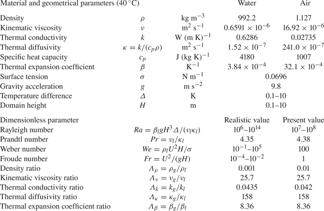
The values of the control parameters are chosen mainly based on the properties of air and water (see table 1), though for better numerical efficiency we take the density ratio  $\varLambda _\rho =0.01$, about $10$ times larger than in reality. Note that the exact value of this parameter hardly affects our results. As the bubbles are pinned and the buoyancy and surface tension forces applied on bubbles are always balanced, we take $Fr=1$ and $We=100$, also for numerical convenience. The geometrical parameters of the bubbles are the relative covered area $0.18\leqslant S_0\leqslant 0.62$, the non-dimensionalised height $0.02\leqslant h/H\leqslant 0.05$, their number $40\leqslant n\leqslant 144$, and the spatial distribution (uniform, random and half-covered). Note that from $S_0$, $\tilde {h}=h/H$ and $n$, we can also calculate the bubble volume ( $=S_0 \tilde {h}/2+n {\rm \pi}\tilde {h}^3/6$), the bubble contact radius ( $=\sqrt {S_0/(n{\rm \pi} )}$) and the bubble contact angle ( $=\arccos \{[S_0/(2n{\rm \pi} \tilde {h})-\tilde {h}/2]/[S_0/(2n{\rm \pi} \tilde {h})+\tilde {h}/2]\}$). As the local Weber number of the bubble is relatively low due to the small bubble size, the bubbles maintain their spherical-cap shape although the bubbles could deform and the flows inside and outside the bubbles are both solved. The bubble shape is closer to spherical with larger $\tilde {h}$ and smaller $S_0/n$.
To ensure that the contact lines are pinned on the plate, we set the value of  $C$ on the hot bottom plate equal to the initial value as the boundary condition of the phase field. The other boundary conditions are no-slip velocities on the top and bottom plates, fixed temperature $\theta _{cold}=0$ (top) and $\theta _{hot}=1$ (bottom) and periodic conditions in the horizontal directions. Stretched grids with $288^3$ gridpoints are used for the velocity and temperature fields, and uniform grids with $576^3$ gridpoints for the phase field (Liu et al. Reference Liu, Ng, Chong, Verzicco and Lohse2021), which corresponds to at least $12$ gridpoints used for the bubble height. The mesh is sufficiently fine and is comparable to corresponding single-phase studies (Stevens, Verzicco & Lohse Reference Stevens, Verzicco and Lohse2010; van der Poel, Stevens & Lohse Reference van der Poel, Stevens and Lohse2013).
3. Flow features and heat transfer
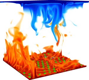
A typical thermal structure in RB convection with bubbles attached to the hot plate is shown in figure 1. Although there is continuous emission of thermal plumes, the bubbles almost maintain the shape of spherical cap due to the pinned contact lines and sufficiently strong surface tension. This is indeed the relevant situation during most of the time for the bubbles in electrolysis or catalysis. In figures 1(a) and 1(b), we observe the plumes rising up from the gaps between the bubbles. Inside the bubbles (see the inset in figure 1c), pure thermal conduction takes place because the local Rayleigh number inside the bubble  $\mbox{Ra}_g\approx \beta _g g h^3(\varDelta /2)/(\nu _g\kappa _g)$ is small enough to remain under the onset of convection $\mbox{Ra}_c\approx 1708$ (namely $\mbox{Ra}_g<100$) for all cases. Furthermore, considering that the thermal conductivity of gas is much lower than that of liquid (i.e. for their ratio $\varLambda _k=0.042\ll 1$), the heat transfer through the gas phase is negligible. Therefore, the overall heat-conducting ability of the fluid near the hot bottom plate is lower than that near the cold top plate. Consequently, because the total heat flux is the same across each horizontal plane, the temperature drop across the hot bottom BL becomes larger than that across the cold top BL, leading to the mean centre temperature smaller than $0.5$ (e.g. $0.461$ in figure 1c), closer to the temperature of the cold top plate to that of the hot bottom plate.

Figure 1. RB convection with bubbles on the hot plate for  $\mbox{Ra} = 10^8$, $\mbox{Pr}=4.38$, $S_0=0.18$, $\tilde {h}=0.02$ and $n=144$: (a) volume rendering of a snapshot of the thermal structures, (b) horizontal slice at the height of the lower (hot) BL thickness and (c) mean (over time and space) temperature profile with an inset showing thermal structures inside one bubble. The temperature field is colour-coded and the interface between liquid and gas is marked in green. As seen from the mean temperature profile in (c), due to the bubbles the mean centre temperature $\bar {\theta }=0.461$ is lower than the average temperature $1/2$ of the top and bottom plates (dashed black line).
In figure 2, we plot the heat transfer  $\mbox{Nu}$ (normalised by $\mbox{Nu}_s$ of single-phase system) as function of the geometrical parameters. As shown in figure 2(a), unsurprisingly, $\mbox{Nu}/\mbox{Nu}_s$ decreases with increasing the relative bubble-covered area $S_0$ due to the decreasing conducting area. We also observe that $\mbox{Nu}/\mbox{Nu}_s$ decreases with increasing bubble height $h$ (normalised by the thermal BL thickness $\lambda$) in figure 2(b), since for larger bubbles there is less liquid (the major conducting fluid) in the thermal BL. With increasing $h/\lambda$, the simulation results gradually deviate from the predictions, because the larger $h/\lambda$, the more parts of the bubbles enter the bulk, which gradually deviates from our assumption that bubbles only affect the thermal BL structure.

Figure 2. Nusselt number normalised by that in the single-phase system: (a)  $\mbox{Nu}/\mbox{Nu}_s$ as a function of the relative bubble-covered area $S_0$, where the (relative) bubble height $\tilde {h}=0.02$ and the bubble number $n=40$; (b) $\mbox{Nu}/\mbox{Nu}_s$ as a function of $h/\lambda$ for $S_0=0.32$ and $n=40$, with $\lambda$ being the thermal BL thickness (values taken from the hot bottom BL); (c) $\mbox{Nu}/\mbox{Nu}_s$ as a function of $n$ for $S_0=0.18$ and $\tilde {h}=0.02$, where symbols denote the numerical results and lines the predictions of (4.1) and (5.1a,b)–(5.3), and colours are for $\mbox{Ra}=10^7$ (red), $\mbox{Ra}=3.2\times 10^7$ (blue) and $\mbox{Ra}=10^8$ (black). The orange symbol $+$ and the green symbol $\times$ in (c) denote the cases with random bubbles distribution as shown in (d) and the half-covered distribution as shown in (e). All the other symbols in (a–c) are for the uniform distribution. All error bars and deviations between simulations and predictions are within $5\,\%$.
In contrast to the significant effects of  $S_0$ and $\tilde {h}$ on the heat transfer, $\mbox{Nu}/\mbox{Nu}_s$ is insensitive to the bubble number $n$ (see figure 2c), because $n$ only contributes to the second term in the bubble volume ( $=S_0\tilde {h}/2+n{\rm \pi} \tilde {h}^3/2$), which is of order $O(\tilde {h}^3)$ and, thus, negligible compared with the first term ( $O(\tilde {h})$). We further show the effects of the spatial bubble distribution, including uniform, random, and the half bubble-covered distributions in figure 2(c). With all three types of distribution, the values of $\mbox{Nu}/\mbox{Nu}_s$ are almost the same. This indicates that the overall heat flux is insensitive to the spatial bubble distribution, at least in our model system. This differs from the previous studies (Liu & Zhang Reference Liu and Zhang2008; Jiang et al. Reference Jiang, Zhu, Mathai, Verzicco, Lohse and Sun2018), where the large-scale flow is changed by the solid elements on the plate. The rigid solid surfaces imply no-slip velocity boundary conditions, which affect the flow structure much more than the boundary conditions of continuous velocity and shear stress on the deformable bubble interfaces.
Analogous trends are also found in the relationship between the mean centre temperature  $\bar {\theta }$ and the geometrical parameters, as shown in figure 3. In all cases, the temperature profile is asymmetric due to the bubbles, namely $\bar {\theta }$ is lower than the average temperature $1/2$ between top and bottom plates, as explained previously. The temperature profile can be quantitatively described by $\bar {\theta }$ and the top and bottom thermal BL thicknesses, the values of which are calculated in § 5.

Figure 3. Mean centre temperature  $\bar {\theta }$ as a function of (a) $S_0$, (b) $h/\lambda$ and (c) $n$. All the cases are the same as in figure 2. The dashed line denotes the average temperature $1/2$ of the top and bottom plates. All error bars and deviations between simulations and predictions are within $5\,\%$.
Such an asymmetric temperature profile has already been studied in the context of single-phase RB convection under non-Oberbeck–Boussinesq (NOB) conditions (Ahlers et al. Reference Ahlers, Brown, Fontenele Araujo, Funfschilling, Grossmann and Lohse2006), where in water the viscosity and thermal diffusivity are temperature dependent and smaller at the hot bottom plate than at the cold top plate. Also this leads to an asymmetric temperature profile. Ahlers et al. (Reference Ahlers, Brown, Fontenele Araujo, Funfschilling, Grossmann and Lohse2006) employed an extended Prandtl–Blasius BL theory for the NOB conditions in the two BLs, and coupled them by imposing heat flux conservation. With this they could calculate the centre temperature and the thermal BL thicknesses, which well agree with the experimental results. Note that the analytical calculation must be adapted to be applicable to the situation here, because here the BL flow is not parallel to the plates due to bubbles. In addition, whereas in the NOB case one has no-slip and no-penetration boundary conditions throughout, here on the spherical-cap-shaped bubble interface we have the emerging condition of the velocity and shear stresses continuity. However, as in Ahlers et al. (Reference Ahlers, Brown, Fontenele Araujo, Funfschilling, Grossmann and Lohse2006), we use the concept of heat flux conservation to define the thermal BL thickness (see § 4), and then propose the idea of an equivalent single-phase system to mimic the system with attached bubbles (see § 5).
4. Thermal BL thicknesses
A sketch of the temperature profiles near the plates is displayed in figure 4, where we also show how the thermal BL thicknesses are defined. Near the cold top plate (see figure 4a), the thermal BL thickness  $\lambda _{cold}$ is defined through the usual convenient definition via the slope of the temperature profile at the plate from assuming a pure conductive thermal BL and a well-mixed bulk (Ahlers et al. Reference Ahlers, Brown, Fontenele Araujo, Funfschilling, Grossmann and Lohse2006). As $\lambda _{cold}$ we take that distance from the plate, where the tangent to the temperature profile at the plate reaches the mean centre temperature $\bar {\theta }$. However, this definition cannot be directly applied near the hot bottom plate, due to the bubbles. As the bubbles reduce the area occupied by the liquid, the conducting area varies with $z$. We therefore correct the solution for pure thermal conduction in the hot bottom BL based on heat flux $Q$ conservation,
 \begin{equation} Q=k_l\frac{\partial \theta}{\partial z}[1-S(z,S_0,\tilde{h},n)]=k_l\frac{\bar{\theta}H}{\lambda_{cold}}. \end{equation}
Here, the term on the right-hand side is the heat flux on the cold top plate. The gas-covered area  $S(z,S_0,\tilde {h},n)=\max [(S_0+n{\rm \pi} z \tilde {h})(1-z/\tilde {h}),0]$ is the insulating area, which is defined with the assumption of spherical-cap shaped bubbles.

Figure 4. Sketch of the temperature profile near the (a) cold top and (b) hot bottom plate. The red lines denote the temperature profiles, the black lines the mean centre temperature  $\bar {\theta }$, the blue lines the solution for pure thermal conduction in the BL, that is, (4.1), and the green dashed line the tangent of (4.1) at the intersection. Here, $\theta ^*$ is the intercept of the tangent. We define the dimensional BL thickness near the hot and cold plates as $\lambda _{hot}$ and $\lambda _{cold}$, respectively, that is, the distance from the black dashed lines to the corresponding plate.
The thermal BL thickness near the hot bottom plate  $\lambda _{hot}$ equals the distance from the plate to the intersection between the lines of (4.1) and of $\theta =\bar {\theta }$, as shown in figure 4(b). With these definitions, both values of $\lambda _{hot}$ and $\lambda _{cold}$ are close to each other in all cases (within $10\,\%$), as shown in figure 5. As $\lambda _{hot}$ and $\lambda _{cold}$ are almost the same and $\bar {\theta }<(\theta _{hot}+\theta _{cold})/2$, the temperature variations across the hot bottom BL and the cold top BL are different, which is reflected in that the temperature profile is asymmetric.

Figure 5. Thermal BL thicknesses  $\lambda _{hot}$ (empty symbols) and $\lambda _{cold}$ (filled symbols) of the hot bottom and cold top BLs, respectively, as functions of (a) $S_0$, (b) $h/\lambda$ and (c) $n$. All the cases are the same as in figure 2. All error bars and deviations between simulations and predictions are within $5\,\%$.
5. Predictions for  $\mbox{Nu}$ and the centre temperature using equivalent single-phase RB system

To calculate the heat transfer  $\mbox{Nu}$ and the mean centre temperature $\bar {\theta }$, we propose the idea of using an equivalent single-phase set-up to mimic the system with attached bubbles. To find the equivalent flow, we first obtain the effective temperature at the hot bottom plate. This is done by plotting the tangent of (4.1) at the position of $\lambda _{hot}$, and the obtaining $\theta$-intercept of the tangent as effective temperature $\theta ^*$ (see figure 4b).
Next, we compare the effective temperature  $\theta ^*$ and the mean centre temperature $\bar {\theta }$ in figure 6(a), which shows that $\theta ^*$ approximately equals to $2\bar {\theta }$ (within $\pm$5 %). Thus we assume a nearly equivalent single-phase RB counterpart with $\theta _{hot}=2\bar {\theta }$ and $\theta _{cold}=0$, such that $\bar {\theta }$ is the mean value of temperatures on the two plates, as shown in figure 6(b). Again, we note that $\lambda _{hot}$ is close to $\lambda _{cold}$, based on our definition of the thermal BL thickness in § 3. Thus, we have the following relations:
 \begin{equation} \theta^*=2\bar{\theta},\quad\lambda_{cold}=\lambda_{hot}={\lambda_s}. \end{equation}
Here,  $\lambda _s$ is the thermal BL thickness in the single-phase system, which can be calculated as
 \begin{equation} \lambda_s=\frac{H}{2\mbox{Nu}_e}, \end{equation}
where  $\mbox{Nu}_e$ is the heat transfer estimated from the GL theory (Grossmann & Lohse Reference Grossmann and Lohse2000, Reference Grossmann and Lohse2001) for the equivalent single-phase system with $\mbox{Ra}^*=2\bar {\theta }\mbox{Ra}$, $\theta _{hot}=2\bar {\theta }$ and $\theta _{cold}=0$. In the two-phase system and the equivalent single-phase system, the dimensional heat transfer $Q$ (
$Q$ ( $=\mbox{Nu}\,k(\theta _{hot}-\theta _{cold})/H$) should be the same, which yields
 \begin{equation} \mbox{Nu}(\mbox{Ra},\mbox{Pr},S_0,\tilde{h},n)=2\bar{\theta} \mbox{Nu}_e(\mbox{Ra}^*,\mbox{Pr}), \end{equation}
where  $\mbox{Nu}(\mbox{Ra},\mbox{Pr},S_0,\tilde {h},n)=(\bar {\theta }H)/\lambda _{cold}$ is the heat transfer for the two-phase system.

Figure 6. (a) Comparison between the mean centre temperature  $\bar {\theta }_{sim}$ and the effective temperature $\theta ^*_{sim}$, both taken from simulations. The symbols are the same as in figure 2. The shadow is the zone within ${\pm }5\,\%$. (b) Sketch of the bubble system under consideration and the equivalent single-phase RB system. Here, $\bar {\theta }_{sim}$ and $\theta ^*_{sim}$ are plotted this way to support the existence of the equivalent single-phase system.
Combining (5.1a,b)–(5.3) for the equivalent single-phase RB system with (4.1) in § 4, which are both the relationships between  $\bar {\theta }$ and $\lambda _{cold}$, we can calculate $\bar {\theta }$ and $\lambda _{cold}$ by iteratively solving these two relationships. Finally, the heat transfer in the system with attached bubbles can be calculated by $\mbox{Nu}=(\bar {\theta }H)/\lambda _{cold}$.
We emphasise that with this approach, using the equations above without introducing any free parameter, for given  $\mbox{Ra}$, $\mbox{Pr}$ and bubble geometries, we can now calculate $\mbox{Nu}$, $\bar {\theta }$, $\lambda _{hot}$ and $\lambda _{cold}$. The good agreements between the simulations and the predictions for $\mbox{Nu}$, $\bar {\theta }$, $\lambda _{hot}$ and $\lambda _{cold}$ are shown in figures 2, 3 and 5, respectively, where all deviations between simulations and predictions are within $\pm$5 %.
We further check whether our approach is also applicable for large  $\mbox{Pr}$, which, as explained previously, has relevance to transport phenomena in water electrolysis and catalysis. Water electrolysis and catalysis can both lead to natural convection driven by buoyancy, which originates from the density difference of the solute with different concentrations of the electrolysis or catalysis product. Here, the mass transfer is also characterised by $\mbox{Nu}$, that is, the mass transfer normalised by that with pure diffusion (in this context normally called the Sherwood number $Sh$). The control parameters are the Grashof number (dimensionless strength of the solute driving) $Gr$ and the Schmidt number (the ratio of viscous diffusion and mass diffusion rates) $Sc$, corresponding to $\mbox{Ra}/\mbox{Pr}$ and $\mbox{Pr}$ in RB convection, respectively. The value of $Sc$ in water electrolysis is always large, e.g. $Sc=400$ (Sepahi et al. Reference Sepahi, Pande, Chong, Mul, Verzicco, Lohse, Mei and Krug2022).
We performed two simulations (for two different bubble heights) at  $\mbox{Pr}=400$ and $\mbox{Ra}=10^7$ (tabulated in table 2) with a sufficiently fine mesh as explained in § 2. Note the much higher computational costs at this large $\mbox{Pr}$, due to the required long time ( ${\sim }\mbox{Pr}^{1/2}$) for the system to enter the statistical steady state. The bubble geometries are characterised by $\tilde {h}=0.03$ and $0.05$, $S_0=0.32$ and $n=40$. The good agreements between our parameter free predictions and the results from the simulations are shown in table 2. This supports that our predictions can be directly applied to water electrolysis and catalysis.
Table 2. Comparisons between simulations and predictions at large  $\mbox{Pr}=400$. The other parameters are $\mbox{Ra}=10^7$, $S_0=0.32$ and $n=40$.

6. Conclusions and outlook
Turbulent RB convection with gas bubbles attached to the hot plate is numerically investigated for  $10^7\leqslant \mbox{Ra}\leqslant 10^8$ and $\mbox{Pr}=4.38$ and $400$. The bubble geometrical parameters are the relative bubble-covered area $S_0$, the relative bubble height $\tilde {h}$, the bubble number $n$ and the spatial bubble distribution. Owing to the much lower thermal conductivity of gas as compared with liquid, the temperature profile is asymmetric and the heat transfer efficiency of the system is reduced. More specifically, $\mbox{Nu}$ significantly decreases with increasing $S_0$ and $\tilde {h}$, but is almost unaffected by $n$ and the types of bubble distribution.
To predict the heat transfer and the mean centre temperature of the system, we have proposed the idea of using an equivalent single-phase system to mimic the system with attached bubbles. By applying the GL theory for the equivalent system and imposing heat flux conservation in the two thermal BLs, we can predict the heat transfer, the top and bottom thermal BL thicknesses and the mean centre temperature, without introducing any free parameter. The predictions well agree with the results from the simulations. Briefly, in § 4 we obtained one relationship between  $\bar {\theta }$ and $\lambda$ in (4.1), and in § 5 we obtained another relationship between $\bar {\theta }$ and $\lambda$ in (5.1a,b) and (5.3). Then, for only given $\mbox{Ra}$, $\mbox{Pr}$ and bubble geometries, we can well predict the heat transfer and temperature profile in the system with bubbles attached to the bottom plate.
The results of this study can be used not only for the heat transfer in RB convection with bubbles attached to the plates, but also for the mass transfer in electrolysis or catalysis. Our predictions can help to obtain estimates for relevant applications and, for example, optimise the heat or mass transfer and flow features in systems in which bubbles are forming on the plate(s). It would also be interesting to extend our basic idea to other wall-bounded turbulent systems with various plate properties, such as plates with inhomogeneous properties (e.g. wettability or conducting ability).
Acknowledgements
We acknowledge PRACE for awarding us access to MareNostrum in Spain at the Barcelona Computing Center (BSC) under the project 2021250115 and the Netherlands Center for Multiscale Catalytic Energy Conversion (MCEC). K.L.C. acknowledges support from the Shanghai Science and Technology Program under project no. 19JC1412802.
Declaration of interests
The authors report no conflict of interest.


 Open access