


1. Introduction
Acoustic streaming has been responsible for some of science's greatest controversies, a fickle and complex nonlinear phenomenon used in modern times (Friend & Yeo Reference Friend and Yeo2011; Rufo et al. Reference Rufo, Cai, Friend, Wiklund and Huang2022) to overcome a key challenge in micro- to nano-scale fluid mechanics: the generation of flow. E.F.F. Chladni became quite popular in the late 18th and early 19th centuries, touring between European locations, demonstrating the curious phenomenon of sand collecting into patterns upon surfaces set into vibration by tones produced from a clavicylinder (Musielak Reference Musielak2020), a clever instrument devised by Robert Hooke (of Hooke's law) and lost to time. One of the attendees of Chladni's seminars at the Tuileries Palace in 1809 – among Biot, Poisson, Navier and Napoléon Bonaparte – Félix Savart was also conducting acoustics experiments and found that the Chladni patterns were at times inconsistent, voicing one discrepancy of several that came to define a bitter relationship between the two men (Bell Reference Bell1991). Sand sometimes collected at vibration antinodes instead of nodes, and Savart posited that air flow driven by the acoustic wave propagating in the adjacent vibrating structure was responsible, a view supported by experiments conducted later by Michael Faraday (Reference Faraday1831). Indeed, the complication of acoustic streaming led to a long history of research in this area, perhaps finally resolved approximately a decade ago (Dorrestijn et al. Reference Dorrestijn, Bietsch, Açıkalın, Raman, Hegner, Meyer and Gerber2007). Ironically, the acoustic streaming enhanced particle collection phenomenon has itself also proved useful to identify the presence of high-frequency acoustic waves now popular for acoustic streaming (Tan, Friend & Yeo Reference Tan, Friend and Yeo2007).
The analysis of acoustic streaming awaited better understanding of the governing equations responsible for conservation of mass and momentum from decades of effort by Navier and Stokes and contemporaries, and the treatment of the coupled nonlinear phenomena in some way to produce a tractable approach. In 1884, Lord Rayleigh devised a small-parameter asymptotic expansion to elegantly separate the conservation equations based on phenomena (Rayleigh Reference Rayleigh1884), with the Mach number as the parameter. The zeroth-order phenomena included hydrodynamics that would be present in the absence of the acoustic wave and the phenomena that it caused, while the first-order terms were intended to represent the linear acoustic field that gave rise to the second-order terms that, after time averaging, produced an estimate for the acoustic streaming. Over the years since, the approach has been both refined (Westervelt Reference Westervelt1951a,Reference Westerveltb; Nyborg Reference Nyborg1965) and applied to specific instances of acoustic streaming, from boundary layer phenomena (Schlichting Reference Schlichting1932) to streaming in one direction driven by progressive attenuation of the acoustic wave along that direction, with the convenience of one-dimensional flow assumptions that eliminated otherwise intractable nonlinear terms that were present due to lateral flow (Eckart Reference Eckart1948). Moreover, the presentation of the analysis has changed to illustrate that acoustic streaming can be viewed as a method for transmitting vorticity (Nyborg Reference Nyborg1965).
Unfortunately, the asymptotic approach has drawbacks. In a seminal paper, Lighthill (Reference Lighthill1978) explained how the requirement of ignoring the streamwise acceleration would suit only what he called slow streaming – streaming in which the acoustic streaming-driven fluid momentum would not be significant in comparison to the acoustic wave responsible for it. A consequence is that nonlinear contributions of acoustic streaming to the acoustic wave are ignored. Before Lighthill, Zarembo (Reference Zarembo1971) also identified problems with the asymptotic expansion approach to slow streaming, suggesting instead that the problem be separated into steady-state and dynamic parts, but with little more to offer the reader in replacing the classic approach. Lighthill notably pointed out that as one increases the frequency of the acoustic wave, the acoustic wave's propagation distance decreases, leading to a more concentrated flow field that can easily exceed the confines of the slow streaming assumptions. In fact, he suggests that 1 MHz acoustic waves adjacent to a wall will form acoustic streaming that exceeds slow streaming assumptions at an acoustic source power of 10 mW.
In the context of modern acoustofluidics, acoustic streaming is typically used beyond an acoustic frequency of 1 MHz and an acoustic source power of 10 mW to obtain the rapid and focused flows desired in applications, and it is not unusual to see 10 MHz to 1 GHz ultrasound at up to an acoustic source power of 10 W in driving acoustic streaming flows. Nonetheless, the classic slow streaming approach remains popular because it is tractable, and few alternatives are known. A good representative of these types of solutions is provided by Vanneste & Bühler (Reference Vanneste and Bühler2011). They published a formal asymptotic expansion in analysis of acoustic streaming driven by surface acoustic waves, with the acoustic Mach number as a small parameter. To obtain convergence, the expansion is later relaxed to accommodate interior streaming that could potentially – and problematically – grow without bound (Orosco & Friend Reference Orosco and Friend2022). Riley (Reference Riley2001) used the inverse of the Strouhal number instead of a Mach number as the small parameter for the asymptotic expansion, putting the disparity in time between the acoustics and the consequent hydrodynamics in control of the expansion. As the disparity increases, the accuracy of Riley's expansion increases. Rudenko & Soluyan (Reference Rudenko and Soluyan1971) provided another approach, separating the acoustic and hydrodynamic phenomena in time via the differential operators used to define the conservation of mass and momentum, though only in a qualitative fashion. However, this style of approach was adopted by Chini, Malecha & Dreeben (Reference Chini, Malecha and Dreeben2014) to produce a complete and useful solution for slow acoustic streaming. Nama, Huang & Costanzo (Reference Nama, Huang and Costanzo2017) use arbitrary Lagrangian–Eulerian analysis of a slow streaming system with acoustic and hydrodynamic spatial scales that are similar to each other. They made use of work by Xie & Vanneste (Reference Xie and Vanneste2014) to expose explicitly the difference in the time scales of the acoustic and hydrodynamic phenomena, and define them to be similar.
An alternative is to simply apply direct numerical simulations (DNS) of the full mass and momentum conservation equations to the problem, resorting to brute force and computational power. Unfortunately, the spatiotemporal separation between the acoustic waves and the hydrodynamic flow that they drive – some 5–9 orders of magnitude (Orosco & Friend Reference Orosco and Friend2022) – is sufficient to prevent adequate DNS solution of even simple problems without assumptions. A typical problem is estimated to take years to solve on today's computers unless some weakening assumptions are made to eliminate boundary layers and free fluid interfaces (Rezk, Yeo & Friend Reference Rezk, Yeo and Friend2014b).
Here, we seek to produce equations to represent nonlinear periodic flow, e.g. an acoustic wave or an ocean surface wave, and their culmination in a steady-state flow of arbitrary Reynolds number at long times – fast acoustic streaming – where we account for the convection of momentum in and between the periodic and steady components of the flow, extending the equations for slow streaming to account for finite Reynolds number streaming. In § 2, we extend the ideas of Zarembo (Reference Zarembo1971) and convert the Navier–Stokes and continuity equations to two dependent systems of equations, one for periodic flow and the other for steady flow. In § 3, we use characteristics of the physical parameters in our problem to render the equations dimensionless, discuss the governing dimensionless parameters, and give scaling insights about the level of nonlinear effects in the steady and periodic flow components. In § 4, we look at a case study of acoustic streaming generated near an acoustic horn, where we follow the simplifying guidelines of Rudenko & Soluyan (Reference Rudenko and Soluyan1971), to demonstrate that our equations are compatible with slow streaming and highlight characteristic properties of fast streaming at moderate and large Reynolds numbers. Finally, we summarize and conclude our findings in § 5.
2. Theory
In our analysis to follow, we obtain fast acoustic streaming equations. We use explicitly three postulates that form the backbone of Eckart (Reference Eckart1948) slow acoustic streaming and many published works reliant upon it. First, we postulate that the flow field parameters – the fluid's velocity  $\boldsymbol {u}$, pressure
  $p$, and density
  $\rho$ – are the sum of steady and periodic/transient components. Specifically, we postulate that
 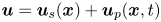 $\boldsymbol {u}=\boldsymbol {u}_s(\boldsymbol {x})+\boldsymbol {u}_p(\boldsymbol {x},t)$. The steady component is
  $\boldsymbol {u}_s(\boldsymbol {x})$, denoted with a subscript
  $s$ and solely a function of the spatial coordinates
  $\boldsymbol {x}$, while
  $\boldsymbol {u}_p(\boldsymbol {x},t)$ is the transient component of the flow, denoted with a subscript
  $p$, and is also a function of time
  $t$. The pressure and density are similarly
  ${p}=p_s(\boldsymbol {x})+p_p(\boldsymbol {x},t)$ and
  $\rho =\rho _s+\rho _p(\boldsymbol {x},t)$. Second, we assume that the transient components are periodic in time and satisfy one angular frequency
  $\omega$, or at most a finite set of angular frequencies indexed with
  $i=1,2,3,\ldots$ such that the periodic flow frequency group may be represented by
  $\sum _i\omega _i$. Hence
  $(1/\tau )\int _{t'=0}^\tau \boldsymbol {u}(\boldsymbol {x},t')\,{\rm d}t'\equiv \left \langle \boldsymbol {u}(\boldsymbol {x},t)\right \rangle =\boldsymbol {u}_s(\boldsymbol {x})$,
  $\left \langle \,p\right \rangle =p_s(\boldsymbol {x})$ and
  $\left \langle \rho \right \rangle =\rho _s$, where
  $\tau \gg \omega _i^{-1}$ is considered a long time with respect to the period
  $2{\rm \pi} /\omega _i$ (for any value
  $i$) of the periodic flow. For example, in many modern acoustofluidic applications, a mono-frequency acoustic wave propagates through a fluid at frequency range
  $\omega _1=10^6\unicode{x2013}10^8$ Hz, which translates to a corresponding periodic time in the range
  $\omega _1^{-1}=10^{-6}\unicode{x2013}10^{-8}\ \text {s}$. Third, we assume a small Mach number to represent the flow field, so that
  $\rho _s\gg \rho _p$.
We next make an assumption that is at odds with the classic slow streaming literature. The traditional assumption is that the particle velocity of the acoustic wave is much faster than the fluid velocity that it causes via acoustic streaming:  $O(\boldsymbol {u}_p)\gg O(\boldsymbol {u}_s)$. This assumption is key to the expansion of the Navier–Stokes equations in the traditional approach. We instead assume that the periodic and steady flow components (or the particle velocity of the acoustic wave and the acoustic streaming-driven fluid velocity) are of the same order of magnitude:
  $O(\boldsymbol {u}_p)\approx O(\boldsymbol {u}_s)$. This relationship between the two velocities is reasonable in fast acoustic streaming.
The Navier–Stokes and continuity equations
 \begin{equation} \rho\left({\dot{\boldsymbol{u}}}+\boldsymbol{u}\boldsymbol{\cdot}\boldsymbol{\nabla}\boldsymbol{u}\right)=-\boldsymbol{\nabla} p +\mu\,\nabla^2\boldsymbol{u}+\left(\mu/3+\mu_b\right)\boldsymbol{\nabla}\boldsymbol{\nabla}\boldsymbol{\cdot}\boldsymbol{u},\quad \dot{\rho}+\boldsymbol{\nabla}\boldsymbol{\cdot}\left(\rho\boldsymbol{u}\right)=0, \end{equation}
may be averaged over long times ( $t=\tau$) to give an equation for the steady flow component,
 \begin{align} \rho_s\boldsymbol{u}_s\boldsymbol{\cdot}\boldsymbol{\nabla}\boldsymbol{u}_s+\boldsymbol{\nabla} p_s -\mu\,\nabla^2\boldsymbol{u}_s &=-\langle\rho_p\dot{\boldsymbol{u}}_{p}+\rho_s\boldsymbol{u}_p\boldsymbol{\cdot}\boldsymbol{\nabla} \boldsymbol{u}_p\rangle\nonumber\\ &\approx-\rho_s\langle\boldsymbol{u}_p\,\boldsymbol{\nabla}\boldsymbol{\cdot} \boldsymbol{u}_p+\boldsymbol{u}_p\boldsymbol{\cdot}\boldsymbol{\nabla}\boldsymbol{u}_p\rangle, \quad \boldsymbol{\nabla}\boldsymbol{\cdot}\boldsymbol{u}_s\approx 0, \end{align}
where we neglect the terms  $\langle \boldsymbol {\nabla }\boldsymbol {\cdot }(\rho _p\boldsymbol {u}_p)\rangle$ and
  $\langle \rho _p\boldsymbol {u}\boldsymbol {\cdot }\boldsymbol {\nabla }\boldsymbol {u}\rangle$; these terms are small compared to
  $\left \langle \boldsymbol {\nabla }\boldsymbol {\cdot }(\rho _s\boldsymbol {u}_s)\right \rangle$ and
  $\left \langle \rho _s\boldsymbol {u}\boldsymbol {\cdot }\boldsymbol {\nabla }\boldsymbol {u}\right \rangle$, respectively, since
  $\rho _s\gg \rho _p$. This equation is similar to equation (39) obtained by Zarembo (Reference Zarembo1971). We detail the derivation of (2.2) in Appendix A, and show in Appendix B that averaging a periodic property over long times gives a similar result whether or not the time of averaging
  $\tau$ is an integer multiple of the period. We also show in Appendix B that
  $\langle \rho _p\dot {\boldsymbol {u}}_{p}\rangle \approx \langle \boldsymbol {u}_p\boldsymbol {\cdot }\boldsymbol {\nabla }\boldsymbol {u}_p\rangle$. Moreover, the term
  $\langle \boldsymbol {\nabla }\boldsymbol {\cdot }(\rho _p\boldsymbol {u}_p)\rangle$ that we neglect when deriving the leading-order result for the continuity equation (
 $\boldsymbol {\nabla }\boldsymbol {\cdot }\boldsymbol {u}_s\approx 0$) in (2.2) accounts for contributions to the steady flow from density variations (compressibility). Hence, while the leading-order result for the steady flow component, given above, is incompressible, higher-order corrections to this flow will account for the neglected term in the continuity equation. A discussion about compressible acoustic streaming is given elsewhere (Pavlic & Dual Reference Pavlic and Dual2021).
As a further note, the steady component of pressure,  $p_s$, is associated with pressure generated by an external source or by the boundaries of the fluid system. Steady Reynolds stress contributions, such as acoustic radiation pressure to appear along the path of an acoustic wave (Chu & Apfel Reference Chu and Apfel1982), are accounted for on the right-hand side of the equality in the conservation of momentum equation in (2.2); this is a gradient of the Reynolds stress in the fluid. Moreover, while in this work we are not concerned with the effects of Reynolds stress at boundaries, it is useful to note a flow stress boundary condition unique to acoustic systems, which is a product of Reynolds stress: an acoustic wave travelling through fluid phases of different acoustic impedance
  $\rho _s\omega /\kappa$ imposes net stress at their interface (Rajendran et al. Reference Rajendran, Jayakumar, Azharudeen and Subramani2022).
Subtracting (2.2) from (2.1a,b) gives an equation for the periodic flow:
 \begin{equation} \left.\begin{gathered} \rho_s{\dot{\boldsymbol{u}}_{p}}+\boldsymbol{\nabla} p_p -\mu\,\nabla^2\boldsymbol{u}_p-\left(\mu/3+\mu_b\right) \boldsymbol{\nabla}\boldsymbol{\nabla}\boldsymbol{\cdot}\boldsymbol{u}_p=\boldsymbol{F},\quad \text{where}\\ \boldsymbol{F}/\rho_s\equiv-\boldsymbol{u}_p\boldsymbol{\cdot}\boldsymbol{\nabla} \boldsymbol{u}_p+\langle\boldsymbol{u}_p\,\boldsymbol{\nabla}\boldsymbol{\cdot} \boldsymbol{u}_p+\boldsymbol{u}_p\boldsymbol{\cdot}\boldsymbol{\nabla}\boldsymbol{u}_p\rangle- \boldsymbol{u}_s\boldsymbol{\cdot}\boldsymbol{\nabla}\boldsymbol{u}_p-\boldsymbol{u}_p\boldsymbol{\cdot} \boldsymbol{\nabla}\boldsymbol{u}_s\\ {}-\frac{\rho_p}{\rho_s}({\dot{\boldsymbol{u}}_{p}}+\boldsymbol{u} \boldsymbol{\cdot}\boldsymbol{\nabla}\boldsymbol{u})\quad \text{and} \quad \dot{\rho}_p+\rho_s(\boldsymbol{\nabla}\boldsymbol{\cdot}\boldsymbol{u}_p)\approx 0, \end{gathered}\right\} \end{equation}
where again we neglect the term  $\langle \boldsymbol {\nabla }\boldsymbol {\cdot }(\rho _p\boldsymbol {u}_p)\rangle$ in the continuity equation.
Assuming that the periodic pressure component  $p_p$ is driven solely by acoustic effects, it becomes reasonable to define an equation of state as an adiabatic relationship between the pressure and density such that
  $p-p_s\approx c^2(\rho -\rho _s)$, where
  $c$ is the phase velocity of the periodic flow. This relationship translates to the expression
  $p_p\approx c^2\rho _p$, that when substituted into the continuum equation in (2.3) produces
 \begin{equation} \dot{p}_p/c^2\approx-\rho_s\,\boldsymbol{\nabla}\boldsymbol{\cdot}{u_p}. \end{equation}
Substituting (2.4) in the time derivative of the conservation of momentum equation in (2.3) gives
 \begin{align} \left.\begin{gathered} \rho_s\ddot{\boldsymbol{u}}_{p}-c^2\rho_s\,\boldsymbol{\nabla}\boldsymbol{\nabla}\boldsymbol{\cdot} \boldsymbol{u}_p -\mu\,\nabla^2\dot{\boldsymbol{u}}_{p}-\left(\mu/3+\mu_b\right) \boldsymbol{\nabla}\boldsymbol{\nabla}\boldsymbol{\cdot}\dot{\boldsymbol{u}}_{p}=\dot{\boldsymbol{F}},\\ \dot{\boldsymbol{F}}/\rho_s\equiv-\dot{\boldsymbol{u}}_{p}\boldsymbol{\cdot}\boldsymbol{\nabla} \boldsymbol{u}_p-\boldsymbol{u}_p\boldsymbol{\cdot}\boldsymbol{\nabla}\dot{\boldsymbol{u}}_{p} -\boldsymbol{u}_s\boldsymbol{\cdot}\boldsymbol{\nabla}\dot{\boldsymbol{u}}_{p}- \dot{\boldsymbol{u}}_{p}\boldsymbol{\cdot}\boldsymbol{\nabla}\boldsymbol{u}_s- \frac{\dot{\rho}_p}{\rho_s}({\dot{\boldsymbol{u}}_{p}}+\boldsymbol{u} \boldsymbol{\cdot}\boldsymbol{\nabla}\boldsymbol{u})-\frac{\rho_p}{\rho_s}\,\ddot{\boldsymbol{u}}_{p}, \end{gathered}\right\} \end{align}
where we neglect small terms that are proportional to  ${\rho _p}/{\rho _s}\ll 1$, and where
  $(\partial /\partial t)\langle \boldsymbol {u}_p\,\boldsymbol {\nabla }\boldsymbol {\cdot } \boldsymbol {u}_p+\boldsymbol {u}_p\boldsymbol {\cdot }\boldsymbol {\nabla }\boldsymbol {u}_p\rangle =0$ since it is a steady quantity in (2.2). There are two interesting terms in this equation: the first is
  ${\dot {\rho }_p}/{\rho _s}$, and the other is
  $({\rho _p}/{\rho _s})\ddot {\boldsymbol {u}}_{p}$. Rearranging the continuity equation in (2.3) produces
  ${\dot {\rho }_p}/{\rho _s}\approx -\boldsymbol {\nabla }\boldsymbol {\cdot }\boldsymbol {u}_p$. Hence
  ${\dot {\rho }_p}/{\rho _s}$
  $({\dot {\boldsymbol {u}}_{p}}+\boldsymbol {u}\boldsymbol {\cdot }\boldsymbol {\nabla } \boldsymbol {u})\,\approx -\boldsymbol {\nabla }\boldsymbol {\cdot }\boldsymbol {u}_p{\dot {\boldsymbol {u}}_{p}}- \boldsymbol {\nabla }\boldsymbol {\cdot }\boldsymbol {u}_p\boldsymbol {u}_s \boldsymbol {\cdot }\boldsymbol {\nabla }{\boldsymbol {u}_s}-\boldsymbol {\nabla }\boldsymbol {\cdot } \boldsymbol {u}_p\boldsymbol {u}_s\boldsymbol {\cdot }\boldsymbol {\nabla }{\boldsymbol {u}_p}- \boldsymbol {\nabla }\boldsymbol {\cdot }\boldsymbol {u}_p\boldsymbol {u}_p \boldsymbol {\cdot }\boldsymbol {\nabla }{\boldsymbol {u}_s}- \boldsymbol {\nabla }\boldsymbol {\cdot }$
  $\boldsymbol {u}_p\boldsymbol {u}_p\boldsymbol {\cdot }\boldsymbol {\nabla }{\boldsymbol {u}_p}$. Moreover, integrating over the continuity equation in (2.3) in time gives
  $({\rho _p}/{\rho _s})\ddot {\boldsymbol {u}}_{p}\approx -\ddot {\boldsymbol {u}}_{p}\int _{t'=0}^t\boldsymbol {\nabla }\boldsymbol {\cdot }\boldsymbol {u}_p\,\textrm {d}t'$ for the initial condition
  $\rho _p(t=0)=0$. Substituting this integral term in (2.5) gives a formidable differential–integral equation in time. However, we show in Appendix C that
  $({\rho _p}/{\rho _s)}\ddot {\boldsymbol {u}}_{p}\approx -\boldsymbol {u}_p\,\boldsymbol {\nabla }\boldsymbol {\cdot }\dot {\boldsymbol {u}}_{p}$ over long times, subject to our assumptions that
  $\rho _p$ and
  $\boldsymbol {u}_p$ are periodic fields, which produces a simpler equation for the periodic flow:
 \begin{align} \dot{\boldsymbol{F}}/\rho_s&\approx-\dot{\boldsymbol{u}}_{p}\boldsymbol{\cdot}\boldsymbol{\nabla} \boldsymbol{u}_p-\boldsymbol{u}_p\boldsymbol{\cdot}\boldsymbol{\nabla}\dot{\boldsymbol{u}}_{p}+{\dot{\boldsymbol{u}}_{p}}\, \boldsymbol{\nabla}\boldsymbol{\cdot}\boldsymbol{u}_p+\boldsymbol{u}_p\, \boldsymbol{\nabla}\boldsymbol{\cdot}\dot{\boldsymbol{u}}_{p} \nonumber\\ &\quad -\boldsymbol{u}_s\boldsymbol{\cdot}\boldsymbol{\nabla}\dot{\boldsymbol{u}}_{p}- \dot{\boldsymbol{u}}_{p}\boldsymbol{\cdot}\boldsymbol{\nabla}\boldsymbol{u}_s+ \boldsymbol{\nabla}\boldsymbol{\cdot}\boldsymbol{u}_p\boldsymbol{u}_s \boldsymbol{\cdot}\boldsymbol{\nabla}\boldsymbol{u}_s+ \boldsymbol{\nabla}\boldsymbol{\cdot}\boldsymbol{u}_p\boldsymbol{u}_s\boldsymbol{\cdot}\boldsymbol{\nabla}\boldsymbol{u}_p\nonumber\\ &\quad +\boldsymbol{\nabla}\boldsymbol{\cdot}\boldsymbol{u}_p\boldsymbol{u}_p \boldsymbol{\cdot}\boldsymbol{\nabla}\boldsymbol{u}_p+\boldsymbol{\nabla}\boldsymbol{\cdot} \boldsymbol{u}_p\boldsymbol{u}_p\boldsymbol{\cdot}\boldsymbol{\nabla}\boldsymbol{u}_s+O(\rho_p/\rho_s). \end{align}
The first line of this equation is associated with temporal inertia in the periodic flow. The second and third lines represent steady convective contributions to the periodic flow. Equations (2.2), (2.5) and (2.6) govern the steady flow and periodic flow.
3. Scalings and insights
One may scale the problem by using the transformations
 \begin{equation} t\to \omega t,\quad\boldsymbol{u} \to U\boldsymbol{u},\quad p_p\to \rho_s U (\omega/\kappa)p_p,\quad p_s\to \rho_s U^2p_s,\quad \boldsymbol{x} \to \kappa^{-1}\boldsymbol{x}, \end{equation}
where  $\omega$,
  $\kappa$ and
  $U$ are the angular frequency, wavenumber and characteristic velocity of the periodic flow – particle velocity when the periodic flow is an acoustic wave – with phase velocity
  $\omega /\kappa$, and where
  $\rho _s U \omega /\kappa$ and
  $\rho _s U^2$ scale acoustic and inertial pressure, respectively, in the fluid. Substituting the scales in (2.2), (2.4), (2.5) and (2.6) gives
 $$\begin{gather} \dot{p}_p\approx-\boldsymbol{\nabla}\boldsymbol{\cdot}u_p, \end{gather}$$
 $$\begin{gather}\boldsymbol{u}_s\boldsymbol{\cdot}\boldsymbol{\nabla}\boldsymbol{u}_s+ \boldsymbol{\nabla} p_s -\textit{Re}^{-1}\,\nabla^2\boldsymbol{u}_s\approx-\langle \boldsymbol{u}_p\,\boldsymbol{\nabla}\boldsymbol{\cdot}\boldsymbol{u}_p+\boldsymbol{u}_p \boldsymbol{\cdot}\boldsymbol{\nabla}\boldsymbol{u}_p\rangle, \quad \boldsymbol{\nabla}\boldsymbol{\cdot}\boldsymbol{u}_s=0, \end{gather}$$
and
 \begin{equation} \left.\begin{gathered} \ddot{\boldsymbol{u}}_{p}-\boldsymbol{\nabla}\boldsymbol{\nabla}\boldsymbol{\cdot}\boldsymbol{u}_p- \textit{Re}'^{-1}({\nabla}^2\dot{\boldsymbol{u}}_{p}+\delta\,\boldsymbol{\nabla}\boldsymbol{\nabla} \boldsymbol{\cdot}\dot{\boldsymbol{u}}_{p})\approx {St}^{-1}\,\dot{\boldsymbol{F}}_1+{St}^{-2}\, \dot{\boldsymbol{F}}_2,\\ \dot{\boldsymbol{F}}_1\equiv-\dot{\boldsymbol{u}}_{p}\boldsymbol{\cdot}\boldsymbol{\nabla}\boldsymbol{u}_p- \boldsymbol{u}_p\boldsymbol{\cdot}\boldsymbol{\nabla}\dot{\boldsymbol{u}}_{p}+{\dot{\boldsymbol{u}}_{p}}\, \boldsymbol{\nabla}\boldsymbol{\cdot}\boldsymbol{u}_p+\boldsymbol{u}_p\boldsymbol{\nabla}\boldsymbol{\cdot} \dot{\boldsymbol{u}}_{p} -\boldsymbol{u}_s\boldsymbol{\cdot}\boldsymbol{\nabla}\dot{\boldsymbol{u}}_{p}- \dot{\boldsymbol{u}}_{p}\boldsymbol{\cdot}\boldsymbol{\nabla}\boldsymbol{u}_s, \\ \dot{\boldsymbol{F}}_2\equiv\boldsymbol{\nabla}\boldsymbol{\cdot}\boldsymbol{u}_p\boldsymbol{u}_s\boldsymbol{\cdot} \boldsymbol{\nabla}\boldsymbol{u}_s+\boldsymbol{\nabla}\boldsymbol{\cdot}\boldsymbol{u}_p \boldsymbol{u}_s\boldsymbol{\cdot}\boldsymbol{\nabla}\boldsymbol{u}_p+ \boldsymbol{\nabla}\boldsymbol{\cdot}\boldsymbol{u}_p\boldsymbol{u}_p \boldsymbol{\cdot}\boldsymbol{\nabla}\boldsymbol{u}_s+\boldsymbol{\nabla}\boldsymbol{\cdot} \boldsymbol{u}_p\boldsymbol{u}_p\boldsymbol{\cdot}\boldsymbol{\nabla}\boldsymbol{u}_p, \end{gathered}\right\} \end{equation}
where  $\textit {Re}\equiv \rho _s U/\mu \kappa$ is the hydrodynamic Reynolds number,
  $\delta \equiv (\mu /3+\mu _b)/\mu$ is a viscosity ratio parameter,
  $\sqrt {\textit {Re}'}\equiv \sqrt {\rho _s \omega /\mu \kappa ^2}$ is a Womersley number (or the square root of an acoustic Reynolds number) and
  ${St}^{-1}\equiv U\kappa /\omega$ is an inverse Strouhal number, which further satisfies the relation
  $\textit {Re}/\textit {Re}'={St}^{-1}$.
It is of value to show that (3.3a,b) and (3.4) reproduce the classic Eckart (Reference Eckart1948) problem for small  $\textit {Re}$. We rewrite (3.3a,b) in the form
 \begin{equation} {\nabla}^2\boldsymbol{u}_s\approx \textit{Re}\langle\boldsymbol{u}_p\boldsymbol{\nabla} \boldsymbol{\cdot} \boldsymbol{u}_p+\boldsymbol{u}_p\boldsymbol{\cdot}\boldsymbol{\nabla}\boldsymbol{u}_p\rangle +O(\textit{Re}), \quad \boldsymbol{\nabla}\boldsymbol{\cdot}\boldsymbol{u}_s=0, \end{equation}
where the inertial and pressure terms are order of magnitude  $O(\textit {Re})$ and are marked accordingly. Moreover, we rewrite (3.4) in the form
 \begin{equation} \ddot{\boldsymbol{u}}_{p}-\boldsymbol{\nabla}\boldsymbol{\nabla}\boldsymbol{\cdot}\boldsymbol{u}_p- \textit{Re}'^{-1}({\nabla}^2\dot{\boldsymbol{u}}_{p}+\delta\,\boldsymbol{\nabla}\boldsymbol{\nabla}\boldsymbol{\cdot} \dot{\boldsymbol{u}}_{p})\approx0+ O({St}^{-1}), \end{equation}
where the  $O({St}^{-1})$ right-hand side of the equation is marked accordingly. The solution of the wave equation in (3.6) for a harmonic wave travelling along the Cartesian coordinate
  $x$ decays exponentially in space like
  $\exp ({-((1+\delta ) \times \textit {Re}'^{-1}/2)x})$, to leading order. Thus the forcing term
  $\textit {Re}\langle \boldsymbol {u}_p\,\boldsymbol {\nabla } \boldsymbol {\cdot } \boldsymbol {u}_p+\boldsymbol {u}_p\boldsymbol {\cdot }\boldsymbol {\nabla }\boldsymbol {u}_p\rangle$ for the steady flow
  $\boldsymbol {u}_s$ in (3.5a,b) is along the wave path (coordinate
  $x$) and proportional to
  $\textit {Re}/\textit {Re}'={St}^{-1}$. This result is compatible with the classic Eckart-type analysis for slow streaming, which is proportional to
  ${St}^{-1}$. Contributions from transient nonlinear terms in the steady flow equation (3.6) and wave equation (3.5a,b) are order of magnitude
  $O({St}^{-2})$ and customarily are ignored in the classic Eckart-type analysis.
Next, we discuss the connection between large and small Reynolds number ( $\textit {Re}$) flow, i.e. fast and (classic Eckart-type) slow streaming, respectively, and obtain general insights about the periodic and steady components of the flow by assuming characteristic quantities appropriate for modern acoustofluidics in the generation of steady flow – acoustic streaming – in liquid, i.e.
  $\rho _s=10^3\ \textrm {kg}\ \textrm {m}^{-3}$,
  $U=1\ \textrm {m}\ \textrm {s}^{-1}$,
  $\omega =10^7$ Hz,
  $\kappa =10^5\ \textrm {m}^{-1}$,
  $\omega /\kappa =10^3\ \textrm {m}\ \textrm {s}^{-1}$ and
  $\mu =10^{-3}\ \textrm {Pa}\ \textrm {s}$. These assumed values produce
  $\textit {Re}^{-1}=10^{-2}$,
  $\textit {Re}'^{-1}=10^{-5}$ and
  ${St}^{-1}=10^{-3}$. The steady flow in this problem is therefore governed to leading order by the convection of steady momentum and by the time-averaged convection of periodic momentum.
The scaling analysis reiterates the classic result that the attenuation of the periodic flow in the form of a harmonic acoustic wave will become appreciable at approximately  $((1+\delta ) \times \textit {Re}'^{-1}\kappa /2)^{-1}\approx 1$ m away from the acoustic source for the characteristic parameter values given above. This is the leading-order viscous attenuation length of the acoustic wave. Moreover, the cumulative distortion of the periodic flow due to convective effects becomes significant at approximately
  ${St}\,\kappa ^{-1}=10^{-2}\ \textrm {m}= 1$ cm away from the acoustic source. For obtaining the latter insight, we assume the linear accumulation of convective contributions (the order of magnitude
  $O({St}^{-1})$) to the acoustic wave over a wavelength
  $\kappa ^{-1}$ in (3.4) and (3.6). Hence if a fluidic system is longer than
  ${St}\kappa ^{-1}$, which in our analysis translates to a length of at least several centimetres, then one should expect that the periodic flow is distorted by the convection of momentum. Moreover, in modern acoustofluidics, where usually
  $\textit {Re}\geqslant 1$, the contribution of momentum convection to the steady flow component should be considered. We emphasize these insights using the case study below.
4. Case study: axisymmetric flow near an acoustic horn
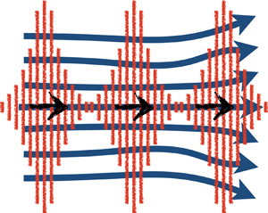
As a simple case study, we consider the two-dimensional Cartesian geometry problem at the line of symmetry in the spirit of Rudenko & Soluyan (Reference Rudenko and Soluyan1971), which we sketch in figure 1. We study the flow between a thickness mode vibrator – an acoustic horn – at  $x=0$, and an acoustic absorber, a solid obstacle of similar acoustic impedance to the fluid in which the acoustic wave propagates, at
  $x=l$. The acoustic horn generates a periodic flow – propagating planar acoustic wave, i.e. a sound or ultrasound wave. The convection of momentum therein produces steady flow – acoustic streaming – at long times. Following the general approach espoused by Rudenko and Soluyan, we then assume a Cartesian axisymmetric system in which the line of symmetry crosses the middle of the acoustic horn surface, and study the flow along this line while approximating lateral viscous contributions. Far from the acoustic horn, the flow is quiescent and the wave vanishes. The simplified model avoids the usual mathematical complexity associated with calculations of steady acoustic streaming flow. The simplicity of the ensuing unidirectional equations emphasizes the principles of fast streaming and a comparison to the classic slow streaming problem by Eckart without the requirement of complex mathematical structures.

Figure 1. A model system that is symmetric about the  $x$ axis, where acoustic waves are generated by an acoustic horn at
  $x=0$, produce acoustic streaming as they attenuate, and absorb in a solid obstacle – an acoustic absorber – at
  $x=l$.
We assume Cartesian coordinates,  $\boldsymbol {x}=(x,y)$, axisymmetric flow with respect to the coordinate
  $x$, given at
  $y=0$, and the steady and periodic flow field vectors
  $\boldsymbol {u}_s=(u,v)$ and
  $\boldsymbol {u}_p=(m,n)$, respectively, where
  $u$ and
  $m$ are flow components along the
  $x$ axis, and
  $v$ and
  $n$ are flow components along the
  $y$ axis. We are interested in approximating the flow from the centre of the acoustic horn and along the axis of symmetry
  $x$ at
  $y=0$. Symmetry requires that
  $v(y=0)=(\partial u/\partial y)|_{y=0}=0$. In addition, we assume that the acoustic wave is quasi-planar near the centre of the horn: its change along the acoustic horn, i.e. along the
  $y$ axis, near the axis of symmetry at
  $y=0$ is negligible, i.e.
  $n=\partial n/\partial y=\partial m/\partial y=\partial ^2 m/\partial y^2=0$ at
  $y=0$; however, the wave vanishes far from
  $y=0$. Using these assumptions, we rewrite the expressions for the steady flow in (3.3a,b) along the axis of symmetry at
  $y=0$:
 $$\begin{gather} u\,\frac{\partial u}{\partial x}+\frac{\partial p_s}{\partial x} -\textit{Re}^{-1}\left(\frac{\partial^2 u}{\partial x^2}+\frac{\partial^2 u}{\partial y^2}\right)\approx-2\left\langle m\,\frac{\partial m}{\partial x}\right\rangle, \end{gather}$$
 $$\begin{gather}\ddot{m}-\frac{\partial^2 m}{\partial x^2} -(1+\delta)\,\textit{Re}'^{-1}\left(\frac{\partial^2 \dot{m}}{\partial x^2}\right)={St}^{-1}\left(-u\,\frac{\partial \dot{m}}{\partial x}-\dot{m}\,\frac{\partial {m}}{\partial x}\right)+O({St}^{-2}), \end{gather}$$
where we ignore second-order  $O({St}^{-2})$ contributions to the acoustic wave in the following, and note that for the leading order,
  $O({St}^{-1})$, convective contributions to the periodic flow,
  $m$, are associated with the steady flow
  $u$.
$u$.
We follow Rudenko & Soluyan (Reference Rudenko and Soluyan1971) and assume that the leading-order flow distribution perpendicular to the axis of symmetry is quadratic,  $u(x,y\to 0)\approx b\,u(x,y=0)\,y^2/2+\cdots$, based on past observations of this type of flow (Dentry, Yeo & Friend Reference Dentry, Yeo and Friend2014). Hence we approximate
  $u_{yy}\approx bu(x,y=0)$, where the friction coefficient
  $b$ is associated with the inverse square of the lateral dimension in this problem, at least near the symmetry line. In the absence of an external pressure field, the hydrodynamic pressure should vanish in the fluid,
  $p_s\equiv 0$, and the approximate system of equations to be solved at the symmetry line at
  $y=0$ becomes
 \begin{equation} u\,\frac{\partial u}{\partial x}-\textit{Re}^{-1}\left(\frac{\partial^2 u}{\partial x^2}-bu\right)\approx-2\left\langle m\,\frac{\partial {m}}{\partial x}\right\rangle \end{equation}
for the steady flow component, and (4.2) for the periodic flow component. The system of equations is subject to the flow quiescent initial conditions  $m(t=0)=({\partial {m}}/{\partial x})|_{t=0}=0$, no-penetration boundary conditions for the steady flow at the surfaces
  $u(x=0)= u(x=l)=0$, and periodic flow boundary conditions
  $m(x=0)=\cos (t)$ and
  $\dot {m}\ + ({\partial {m}}/{\partial x})|_{x=l}=0$ for closure. The first boundary condition represents the assumption that the surface of the acoustic horn at
  $x=0$ vibrates like
  $\cos (t)$. The following boundary condition specifies the presence of an acoustic solid absorber at
  $x=l$ peculiar to this particular model from Rudenko & Soluyan (Reference Rudenko and Soluyan1971), and Eckart (Reference Eckart1948) before them. This condition eliminates wave reflections off its surface by absorbing the incident wave energy instead. In doing so, it produces an ideal sink for the acoustic energy, commonly called today a ‘perfectly matching layer’ along the one-dimensional axis from the source. Such an ideal sink may be used to represent the case where the acoustic source radiates energy into an infinite fluid volume, while avoiding the perceived complexity of the analysis that would entail. By suppressing a returning acoustic wave, it prevents the appearance of interference with the acoustic wave propagating from the source and the consequent generation of a standing wave that would complicate the analysis of the acoustic streaming phenomena.
Eckart slow streaming, where the velocity of streaming is much smaller than that associated with the periodic flow in the acoustic wave, i.e.  $O(u)\ll O(m)$, requires
  $\textit {Re}\ll 1$. Fast streaming, where the streaming velocity may be comparable to the periodic flow in the acoustic wave, i.e.
  $O(u)\approx O(m)$, requires
  $\textit {Re}\gg 1$. Consequently, it is valuable to begin the analysis with an asymptotic treatment for both small and large hydrodynamic Reynolds numbers
  $\textit {Re}$.
4.1. Asymptotic insights
We first consider the asymptotic solution of the equation set (4.2)–(4.3) for small and large  $\textit {Re}$ to assess the steady flow in each case. Unlike
  $\textit {Re}$ that may span a wide range of values that in turn affect the steady flow directly, generally,
  $St$ and
  $\textit {Re}'$ are large numbers associated to leading order with the periodic flow.
4.1.1. Small hydrodynamic Reynolds number ( $\textit {Re}\ll 1$): Eckart slow streaming

In the case of an asymptotically small hydrodynamic Reynolds number ( $\textit {Re}\to 0$), we resurrect the classic Eckart streaming model. In this case, one may ignore to leading order the convection of momentum. The equation set (4.2)–(4.3) is reduced to the leading-order system of equations
 \begin{equation} \frac{\partial^2
u}{\partial x^2} -bu\approx
2\,\textit{Re}\,\Bigl\langle m\,\frac{\partial
{m}}{\partial x}\Bigr\rangle, \quad
\ddot{m}-\frac{\partial^2 {m}}{\partial x^2}
-(1+\delta)\,\textit{Re}'^{-1}\,\frac{\partial^2
\dot{m}}{\partial
x^2}\approx0,
\end{equation}
\begin{equation} \frac{\partial^2
u}{\partial x^2} -bu\approx
2\,\textit{Re}\,\Bigl\langle m\,\frac{\partial
{m}}{\partial x}\Bigr\rangle, \quad
\ddot{m}-\frac{\partial^2 {m}}{\partial x^2}
-(1+\delta)\,\textit{Re}'^{-1}\,\frac{\partial^2
\dot{m}}{\partial
x^2}\approx0,
\end{equation}
with the same boundary and temporal conditions, where the term  $u\,{\partial u}/{\partial x}$ produces second-order contributions to the flow and hence is ignored. The problem in (4.4a,b) is satisfied by the solution
 \begin{equation} \left.\begin{aligned}
m & =\cos{(t-x)}{\rm e}^{-\alpha x}, \cr u & =\frac{{St}^{-1}}{2}\,\frac{(1+\delta)\exp({-2 \alpha
(l+x)-\sqrt{b} x})}{(4 \alpha^2-b) (\exp({2 \sqrt{b} l})-1)} \cr &
\quad\times[- \exp({2 \alpha x+\sqrt{b} l})+\exp({2
\alpha l+\sqrt{b} x})+\exp({2 \alpha (l+x)+2 \sqrt{b}
l})\cr & \quad {}-\exp({2 \alpha (l+x)+2
\sqrt{b} x})-\exp({2 \alpha l+\sqrt{b} (2 l+x)})+ \exp({2
\alpha x+\sqrt{b} (l+2 x)})], \end{aligned}\right\}
\end{equation}
\begin{equation} \left.\begin{aligned}
m & =\cos{(t-x)}{\rm e}^{-\alpha x}, \cr u & =\frac{{St}^{-1}}{2}\,\frac{(1+\delta)\exp({-2 \alpha
(l+x)-\sqrt{b} x})}{(4 \alpha^2-b) (\exp({2 \sqrt{b} l})-1)} \cr &
\quad\times[- \exp({2 \alpha x+\sqrt{b} l})+\exp({2
\alpha l+\sqrt{b} x})+\exp({2 \alpha (l+x)+2 \sqrt{b}
l})\cr & \quad {}-\exp({2 \alpha (l+x)+2
\sqrt{b} x})-\exp({2 \alpha l+\sqrt{b} (2 l+x)})+ \exp({2
\alpha x+\sqrt{b} (l+2 x)})], \end{aligned}\right\}
\end{equation}
where for a small attenuation coefficient  $\alpha \ll 1$, one obtains the classical result
 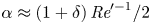 $\alpha \approx (1+\delta )\,\textit {Re}'^{-1}/2$, and where we used the products
 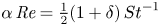 $\alpha \, \textit {Re}=\frac {1}{2}(1+\delta )\,{St}^{-1}$ and
 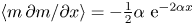 $\left \langle m\,{\partial {m}}/{\partial x}\right \rangle =-\frac {1}{2}\alpha \ \textrm {e}^{-2\alpha x}$. The result in (4.5) re-emphasizes the assumption that the magnitude of the steady flow velocity
  $u$ is much smaller than the particle velocity in the acoustic wave,
  $m$. The ratio of the steady acoustic streaming flow velocity to the particle velocity of the acoustic wave is proportional to
  $St^{-1}\ll 1$.
It is worthwhile to investigate the correction to this problem for a small but finite hydrodynamic Reynolds number ( $\textit {Re}\ll 1$). We assume the asymptotic series for the flow
 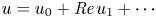 $u=u_0+\textit {Re}\,u_1+\cdots$, which we substitute in (4.3) and the corresponding boundary conditions. The leading-order result (
 $O(1)$) for
  $u_0$ is similar to that given in (4.5). The leading correction (
 $O(\textit {Re})$) to this problem for
  $u_1$ is given by
 \begin{equation} \frac{\partial^2 u_{1}}{\partial x^2}-bu_1=u_0\,\frac{\partial u_{0}}{\partial x}, \end{equation}
subject to the boundary conditions  $u_1(x=0)=u_1(x=l)=0$. While this equation does possess an analytical solution, it is overly convoluted and has limited practical usefulness beyond the contribution of numerical values, which we present in figure 2.

Figure 2. (a) Leading-order ( $u_0$) asymptotic results for small (red) and large (blue) hydrodynamic Reynolds numbers,
  $\textit {Re}$; in the latter, we include the hydrodynamic boundary layer flow near the obstacle (dashed black), which appears here almost as a vertical line at
  $x\approx 30$. We introduce leading-order corrections (b) to the small
  $\textit {Re}$ asymptotic result for various Strouhal numbers,
  $St = \textit {Re}'/\textit {Re}$, and (c) to the large-
 $\textit {Re}$ asymptotic result for various
  $\textit {Re}$. Leading-order results
  $u_0$, and corrections
  $u_1$, are given in red and blue, respectively, and the two first terms in the asymptotic series,
  $u/{St}^{-1}=u_0+{St}^{-1}\,u_1$ and
  $u=u_0+\textit {Re}^{-1/2}\,u_1$ are in black. (d) We further magnify the hydrodynamic boundary layer flow near the wave absorber obstacle for various levels of large
  $\textit {Re}$. In the different results, we assume a linear harmonic acoustic wave and the acoustic attenuation coefficient
  $\alpha =0.01$, and use the friction coefficient
  $b=0.01$ for small
  $\textit {Re}$, and
  $St=0.01$ for large
  $\textit {Re}$.
In figure 2(a), we present the leading-order streaming velocity  $u_0$ in (4.5) between an acoustic horn at
  $x=0$ and a solid wave absorber at
  $x=l\equiv 30$ for an acoustic attenuation length and friction coefficient of the value
  $\alpha =b=0.01$. The flow velocity is proportional to
  ${St}^{-1}$ and reaches a maximum near the acoustic horn, then decaying slowly until it vanishes at the acoustic absorber. In figure 2(b), we demonstrate further the correction to the streaming,
  $u_1$, which is proportional to
  $St^{-2}$ and given in (4.6). The correction due to weak inertia in the streaming delays the streaming spatial variation along the
  $x$ axis. The maximum in the streaming velocity appears further downstream along the
  $x$ axis with increasing
  $\textit {Re}$, and obtains a greater magnitude. Next we consider the asymptotic case of large
  $\textit {Re}$.
4.1.2. Large hydrodynamic Reynolds number ($\textit {Re}\gg 1$): fast streaming

In the case of an asymptotically large  $\textit {Re}$, the convection of momentum governs the streaming away from interfaces. The problem in (4.3) is reduced to
 \begin{equation} u\,\frac{\partial u}{\partial x}\approx-2\,\Bigl\langle m\,\frac{\partial {m}}{\partial x}\Bigr\rangle, \end{equation}
which translates to  $u^2\approx -4\int _{x=0}^{x'}\left \langle m\,{\partial {m}}/{\partial x}\right \rangle {\textrm {d}\kern 0.06em x}+O({St}^{-2})$ subject to the initial condition
  $u(x=0)=0+O({St}^{-1})$. The term
  $O({St}^{-1})$ accounts for boundary layer flow contributions to the bulk flow near the solid surface of the acoustic actuator: since the acoustic streaming is the drift of net mass away from the actuator solid surface, we may not neglect the diffusion of momentum near the solid, especially its component along the actuator solid surface within the viscous boundary layer thickness
  $\sqrt {\mu /\rho _s\omega }$ (Lighthill Reference Lighthill1978; Manor et al. Reference Manor, Dentry, Friend and Yeo2011), where viscous and transient contributions to the flow are comparable. This is a small thickness compared to the acoustic wavelength
  $\kappa ^{-1}$. For example, the viscous boundary layer thickness and acoustic wavelength in ambient water are approximately
  $10^{-7}$–
 $10^{-8}$ m and
  $1.5\times 10^{-3}$–
 $1.5\times 10^{-6}$ m for acoustic frequencies of 1–1000 MHz, respectively. That is, the viscous boundary layer flow appears at
  $x\ll 1$ in our scaled notation. Convection of momentum within the boundary layer flow introduces steady flow – acoustic streaming – of the order of magnitude
  $u=O(St^{-1})$, normal to the finite surface area of the horn. These
  $O({St}^{-1})\ll 1$ surface contributions to the flow are small compared to the magnitude of the
  $O(1)$ fast streaming. Failing to recognize surface contributions to the flow will result in a singular slope of the velocity field near the actuator surface, at
  $x=0$. Specifying a linear acoustic wave propagating away from the actuator, thus substituting the periodic velocity
  $m=\cos (t-x)\ \textrm {e}^{-\alpha x}$ of the wave generated by the actuator alongside, in (4.7) gives
 \begin{equation} u\approx\sqrt{1-{\rm e}^{-2\alpha x}+O({St}^{-2})}, \end{equation}
subject to the approximate boundary condition  $u(x\to 0)= 0+O({St}^{-1})$. This result emphasizes that in this limit, the steady flow velocity
  $u$ should be comparable in magnitude to the particle velocity in the acoustic wave
  $m$, away from the surface of the horn. Both are of the order of magnitude
  $O(1)$ in this scaled analysis.
In the vicinity of the solid acoustic absorber at  $x=l$, viscous dissipation must increase, so that viscous and convective contributions to momentum are comparable, supporting the formation of a classic viscous boundary layer flow near the obstacle. To study the boundary layer flow, we define the stretched coordinate
  $X=(l-x)\,\textit {Re}$, which is opposite the coordinate
  $x$ and originates in the surface of the obstacle, to render comparable the leading-order convective and viscous terms in the steady flow equation. Substituting
  $X$ for
  $x$ in (4.3), and using
  $\tilde {u}(X)$ to indicate flow in the boundary layer, gives
 \begin{equation} \tilde{u}\,\frac{\partial\tilde{u}}{\partial X}+\frac{\partial^2\tilde{u}}{\partial X^2}\approx-\textit{Re}^{-2}\,b\tilde{u}+2\,\textit{Re}^{-1}\,\Bigl\langle m\,\frac{\partial m}{\partial X}\Bigr\rangle, \end{equation}
where  $\left \langle m\,{\partial m}/{\partial X}\right \rangle \approx -\alpha \ \textrm {e}^{-2\alpha l}/2$ in the boundary layer. Ignoring small terms of the order of magnitude
  $O(\textit {Re}^{-1})$ and
  $O(\textit {Re}^{-2})$ on the right-hand side of the equality, we find that
  $\tilde {u}=u(x\to l)\tanh [u(x\to l) X/2]$, where we require that the velocity vanishes at the surface of the obstacle,
  $\tilde {u}(X=0)=0$, and match the flow in the boundary layer to that outside:
  $\tilde {u}(X\to \infty )=u(x\to l)$. Replacing
  $X$ by
  $x$, using (4.8) to identify the term
  $u(x\to l)$, gives the boundary layer flow
 \begin{equation}
\tilde{u}=\sqrt{1-{\rm e}^{-2\alpha l}+O({St}^{-2})}\tanh\,\Bigl(\sqrt{1-{\rm
e}^{-2\alpha
l}+({St}^{-2})}\,\frac{\textit{Re}\,(l-x)}{2}\Bigr),
\end{equation}
\begin{equation}
\tilde{u}=\sqrt{1-{\rm e}^{-2\alpha l}+O({St}^{-2})}\tanh\,\Bigl(\sqrt{1-{\rm
e}^{-2\alpha
l}+({St}^{-2})}\,\frac{\textit{Re}\,(l-x)}{2}\Bigr),
\end{equation}
which highlights rapid viscous diminution of the steady flow close to the obstacle surface. The characteristic dimensionless thickness of the boundary layer is given by  $2/u(x\to l)\,\textit {Re}$; the boundary layer thickness decreases with increasing flow velocity
  $u$ near the absorber surface, and increasing hydrodynamic Reynolds number
  $\textit {Re}$. In particular, approximating
  $u(x\to l)\approx 1$ renders the characteristic length
  $2/\textit {Re}$ smaller than unity for large
  $\textit {Re}$, hence the dimensional length of the viscous boundary layer flow becomes smaller than the acoustic wavelength.
The next and last step that we will take in this subsection is a correction to the steady flow due to small but finite viscous effects, in order to evaluate the leading-order viscous contribution to the flow. For this part, it is sufficient to assume the regular expansion for the corresponding velocity field  $u=u_0+\textit {Re}^{-1/2}\,u_1+\cdots$ in (4.3). The leading-order problem for
  $u_0$ is the same as the equation in (4.7), subject to the same boundary condition at
  $x=0$. The solution for
  $u_0$ is the same as the solution for
  $u$ in (4.8) when assuming that the problem for the acoustic wave
  $m$ is linear, independent of the streaming, and is satisfied by the simple harmonic and exponentially decaying expression in (4.5). The correction to the steady flow of the order of magnitude
  $O(\textit {Re}^{-1/2})$ for
  $u_1$ is given by
  $u_1\,\partial u_{1}/\partial x=\partial ^2 u_{0}/\partial x^2-bu_0$, subject to the initial condition
  $u(x=0)=0$. This problem is satisfied by the integral solution
 \begin{equation} u_1=\sqrt{2\int_{x=0}^{x'} \left(\frac{\partial^2 u_{0}}{\partial x^2}-bu_0\right){{\rm d}\kern 0.06emx}}, \end{equation}
which is valid when the friction coefficient  $b$ is small enough to render the integral positive.
We present the large hydrodynamic Reynolds number  $\textit {Re}$ case in figure 2(a) compared to the small-
 $\textit {Re}$ case. The most striking observation is that while the former case supports an order
  $O(1)$ velocity field – i.e. the steady velocity field is of the same order of magnitude as the particle velocity field in the wave – the velocity field in the latter case is proportional to
  $St^{-1}$, which is a small number in these types of problems, and is weak compared to the particle velocity field in the wave. Correcting the large-
 $\textit {Re}$ result for weak viscous dissipation intuitively reduces the steady flow velocity in a manner proportional to
  $\textit {Re}$. Moreover, close to the wave absorber obstacle, viscous and inertial effects become comparable, which yields the rapid reduction in velocity field that we demonstrate in figure 2(d). In our demonstration, the steady flow loses momentum to viscous dissipation within a fraction of a wavelength, even in the case of moderate
  $\textit {Re}$ values.
Next, we use numerical analysis to study the steady flow and nonlinear acoustic wave at small to moderate and large hydrodynamic Reynolds numbers,  $\textit {Re}$, and further compare our numerical findings for finite
  $\textit {Re}$ to the asymptotic results above.
4.2. Numerical insights
We solve (4.2)–(4.3) and the corresponding boundary and initial conditions to account for finite values of hydrodynamic Reynolds number  $\textit {Re}$ and nonlinear acoustic effects by using finite difference approximations. For the case of low to moderate
  $\textit {Re}$, we employ second-order central difference approximations for spatial and temporal derivatives in the numerical domain, and first-order forward and backward approximations to discretize the boundary and initial conditions. We solve the wave equation in (4.2) using an explicit second-order Newton algorithm, and the boundary value steady flow equation in (4.3) using the matrix algorithm, where we implement a successive over-relaxation approach to facilitate the convergence of the matrix equation at each iterative step of a fixed point iteration algorithm to overcome the nonlinearity of the problem. For the case of large
  $\textit {Re}$, we use the asymptotic equation for
  $u$ in (4.7), and solve the wave equation as in the previous case. We solve the numerical problem between an acoustic horn at
  $x=0$ and a solid wave absorber at
  $x=l\equiv 30$, and average over the acoustic forcing term
  $\left \langle m\,{\partial m}/{\partial x}\right \rangle$ over 15 temporal cycles of the periodic flow
  $m$. Moreover, we employ 1890 spatial numerical nodes and 3780 temporal numerical nodes for small to moderate hydrodynamic Reynolds numbers,
  $\textit {Re}\leq 1$, and 756 spatial numerical nodes and 1512 temporal numerical nodes for the large hydrodynamic Reynolds number case,
  $\textit {Re}\gg 1$. Finally, we require a maximum relative numerical error of 1 % in our results, which we calculate using an infinity norm.
4.2.1. Small to moderate hydrodynamic Reynolds number, $\textit {Re}\leq 1$

First, considering the case of a small to moderate hydrodynamic Reynolds number,  $\textit {Re}\leq 1$, we solve (4.2) and (4.3) for an acoustic Reynolds number and a friction coefficient
  $\textit {Re}'=b=0.01$, and a bulk-to-shear viscosity ratio
  $\delta =1$. In figure 3(a), we present the asymptotic result for small
  $\textit {Re}$ in (4.5), and numerical results for
  $\textit {Re}=0.1, 0.25, 0.5, 0.75, 1$. Our numerical analysis is almost indistinguishable from the asymptotic result for a hydrodynamic Reynolds number
  $\textit {Re}=0.1$. Increasing
  $\textit {Re}$ to unity spatially delays the maximum steady velocity field downstream, which we observe in our asymptotic analysis, where we introduced a correction for small but finite
  $\textit {Re}$.

Figure 3. Spatial ( $x$) variations of (a) acoustic streaming velocity
  $u$ for low and moderate Reynolds number,
  $\textit {Re}$, in comparison to the asymptotic result for
  $\textit {Re}\rightarrow 0$, and a comparison between the spatiotemporal periodic flow
  $m$ in a (red) linear acoustic wave (independent of acoustic streaming) against (blue) its nonlinear counterpart for (b)
  $\textit {Re}=1$ and (c)
  $\textit {Re}=0.01$, in addition to the sum of acoustic streaming
  $u$ and the spatiotemporal periodic flow
  $m$ in a nonlinear acoustic wave for (d)
  $\textit {Re}=1$, (e)
  $\textit {Re}=0.5$ and (f)
  $\textit {Re}=0.1$, where in all cases, excluding the asymptotic analysis, we set the Strouhal number to
  $St = 10$.
In figures 3(b,c), we demonstrate the contribution of steady flow to the periodic flow – the acoustic wave in this case. The contribution may become apparent for sufficiently large  $\textit {Re}$ at (the dimensionless)
  $x>{St}$; this insight is compatible with our discussion in § 3. Moreover, while in practice
  $St=\textit {Re}'/\textit {Re}$, we artificially set the Strouhal number in our numerical calculations to
  $St =10$ to observe this contribution within our numerical region
  $0< x<30$. We show the analytical result for the linear acoustic wave
  $m=\cos (t-x)\ \textrm {e}^{-\alpha x}$ in red, and the numerical result for
  $\textit {Re}=1$ and 0.01 in blue. It is immediately apparent that the acoustic wavelength changes in the case
  $\textit {Re}=1$ due to a Doppler effect: The steady flow ‘pushes’ the acoustic wave along the
  $x$ axis, which results in the linear analytical wave (red) undergoing an additional half period relative to the nonlinear numerical wave (blue), within the same numerical region. Hence the wavelength of the numerical wave increases slightly. In the case
  $\textit {Re}=0.01$, we observe the same number of periodic spatial cycles in both the linear and nonlinear waves. Here, the steady flow is weaker than in the previous case by a factor
  $1/100$ (the ratio between the two corresponding values of
  $\textit {Re}$), hence the ‘push’, which the acoustic wave is getting from the steady flow, is much weaker.
We further plot the sum of the steady and periodic flows,  $u$ and
  $m$, respectively, in figures 3(d–f) for hydrodynamic Reynolds numbers
  $\textit {Re}=1$, 0.5 and 0.1. We observe comparable contributions to the overall flow field from both
  $u$ and
  $m$ for
  $\textit {Re}=1$. However, in the case
  $\textit {Re}=0.1$, the contribution of
  $u$ to the overall flow field is small, since it is proportional to
  $\textit {Re}$. It becomes apparent only at long times following the exclusion of the periodic flow due to long time averaging. We demonstrate the transition between these two cases using
  $\textit {Re}=0.5$, where the contribution of the steady flow to the overall flow is appreciable but to a lesser extent relative to the case
  $\textit {Re}=1$.
We thus find that the asymptotic result for small  $\textit {Re}$ (where we assume a linear acoustic wave) models the flow and acoustic wave well for
  $\textit {Re}\leq 1$: this is an application of the classic Eckart approach for slow streaming. This is not the case for
  $\textit {Re}\gg 1$, which we discuss next.
4.2.2. Large hydrodynamic Reynolds number, $\textit {Re}\gg 1$

We now consider the case of a large hydrodynamic Reynolds number,  $\textit {Re}\gg 1$. We use a similar approach as in the previous case to solve (4.2) for the periodic flow, and integrate (4.7) to solve for the corresponding steady flow in the limit of large
  $\textit {Re}$, assuming an acoustic Reynolds number and a friction coefficient
  $\textit {Re}'=b=0.01$, and a bulk to shear viscosity ratio
  $\delta =1$. In figure 4(a), we present the asymptotic result for large
  $\textit {Re}$ in (4.8), and numerical results for
  ${St}=10$ and 100. The slightly wiggly numerical results in this case are due to our finite time averaging: the longer time we average over the forcing term for the steady flow, the more we eliminate spatial oscillations in the steady flow. We alter the magnitude of
  ${St}$ in this problem to highlight its contribution to the acoustic wave, and observe that our numerical results are similar to the asymptotic result for steady flow. Hence spatiotemporal variations in the nonlinear acoustic wave with
  ${St}$ in our calculations result in small integral contributions to the steady flow.

Figure 4. Spatial ( $x$) variations of (a) acoustic streaming velocity
  $u$ for different values of the Strouhal number
  $St$, and a comparison between the spatiotemporal periodic flow
  $m$ in a (red) linear acoustic wave (independent of acoustic streaming) against (blue) its nonlinear counterpart for (b)
  $St = 10$ and (c)
  $St = 100$, in addition to the sum of acoustic streaming
  $u$ and the spatiotemporal periodic flow in a nonlinear acoustic wave
  $m$, for (d)
  $St = 10$, where in all cases we assume the large-Reynolds-number
  $\textit {Re}\rightarrow \infty$ asymptotics for
  $u$.
$u$.
We compare the nonlinear numerical and linear analytical results for the wave in figures 4(b,c). For a Strouhal number  $St = 10$, the contribution of the steady flow to the acoustic wave becomes apparent at
  $x>St$ in this dimensionless analysis, where the Doppler contribution of the steady flow to the wave becomes appreciable: the nonlinear wave (blue) retains greater magnitude of oscillations than the linear wave (red), sustaining weaker attenuation. Moreover, the change in the wavelength is such that the nonlinear wave undergoes one less periodic spatial cycle than the linear wave in our numerical region. Changing the Strouhal number to
  $St = 100$ suggests that contributions to the wave should become less appreciable within our numerical region
  $0< x<30$. Indeed, in this case the difference between the numerical nonlinear wave (blue) and the linear analytical wave (red) is smaller. Further, we show the sum of the steady and acoustic wave flow fields in figure 4(d) for
  $St = 10$. Here, the sum of the steady and periodic flow components indicates that far from the origin of the acoustic wave – the acoustic horn – where the acoustic wave has mostly attenuated, the flow field as a whole is governed mostly by the steady flow even without time averaging the overall flow field. This result is qualitatively different to the corresponding results that we showed for small
  $\textit {Re}$, where the acoustic wave appears to dominate the flow at any separation from the acoustic horn.
5. Summary and conclusions
In this study, we go back to a problem in acoustofluidics put forward by Zarembo (Reference Zarembo1971) a little more than half a century ago: how should one obtain a tractable solution for a periodic flow ( $\boldsymbol {u}_p$) that supports the presence of a steady flow (
 $\boldsymbol {u}_s$) of similar magnitude? The flow components interact through the convection of momentum, thus circumventing the mostly intractable requirement to solve the full Navier–Stokes equation over long times, while retaining reasonable spatial and temporal resolutions over the periods and wavelengths associated with
  $\boldsymbol {u}_p$ for practical problems. This problem captures the difficulty in predicting fast acoustic streaming: the generation of acoustic streaming (or any steady flow) of finite hydrodynamic Reynolds number,
  $\textit {Re}$, due to convective effects in an acoustic wave (or any periodically varying flow), while the wave is altered simultaneously by the streaming.
In the absence of a general solution to this problem, most current theories for acoustic streaming in a fluid bulk follow the guidelines set by Eckart (Reference Eckart1948), calculating slow acoustic streaming in the asymptotic limit of small  $\textit {Re}$, characterizing the contributions of Rayleigh (Reference Rayleigh1884), Eckart, Nyborg (Reference Nyborg1965), Westervelt (Reference Westervelt1951a) and, more recently, Chini et al. (Reference Chini, Malecha and Dreeben2014) and Nama et al. (Reference Nama, Huang and Costanzo2017), described in the Introduction. The theory by Eckart predicts a linear independent acoustic wave that powers viscous acoustic streaming. However, it is the experience of the authors that, at least in the case of MHz frequency acoustic actuation of streaming (steady flow) in their laboratories, one is not able to observe (low-
 $\textit {Re}$) Eckart streaming in water and other simple liquids using the naked eye; the streaming is too slow. For example, let us assume the kinematic viscosity of water, which is approximately
  $\mu /\rho \approx 10^{-6}\ \textrm {m}^2\ \textrm {s}^{-1}$, and the range of acoustic wavelengths in water in the MHz frequency regime, which is approximately
  $\kappa ^{-1}\approx 10^{-4}$ m. Assuming that the magnitude of the hydrodynamic Reynolds number is sufficiently small to support classic Eckart streaming, e.g.
  $\textit {Re} \approx 0.1$, the corresponding periodic flow (or particle velocity of the acoustic wave) amplitude is approximately
  $U\approx 0.01\ \textrm {m}\ \textrm {s}^{-1}$. The slow Eckart streaming under these conditions is proportional to
  $St^{-1}U\equiv U^2/(\omega /\kappa )$; the phase velocity of the acoustic wave in ambient water is
  $\omega /\kappa \approx 1500\ \textrm {m}\ \textrm {s}^{-1}$. Hence the corresponding acoustic streaming velocity is approximately
  $St^{-1} U\approx (0.01^2 \ \textrm {m}^2\ \textrm {s}^{-2})/(1500\ \textrm {m}\ \textrm {s}^{-1})\approx 10^{-7}\ \textrm {m}\ \textrm {s}^{-1}$.
Another difficulty in observing slow Eckart streaming is the Westervelt paradox (Chu & Apfel Reference Chu and Apfel1982). The paradox is associated with an Eulerian representation of the conservation of momentum and mass in a travelling acoustic wave in fluid: a steady flow – acoustic streaming – is generated opposite the travelling wave path, satisfying a magnitude  $St^{-1}\,U\equiv U^2/(\omega /\kappa )$, and apparently penetrating the solid surface of the periodic flow (or acoustic wave) actuator. A Lagrangian representation of the flow circumvents the paradox by accounting appropriately for fluid density variations, showing that fluid mass does not actually penetrate into the solid actuator. However, the apparent net flow towards the solid actuator is measurable (in an Eulerian – laboratory – frame of view), and advects objects to the surface of the actuator. Hence similar magnitudes of apparent steady flows are generated by slow Eckart streaming and by the Westervelt paradox along and opposite the path of the wave, respectively.
However, many times, one observes acoustic streaming velocities that are  $10^{-3}-1\ \textrm {m}\ \textrm {s}^{-1}$ in magnitude and are comparable to the periodic flow velocity (
 $U$) – the acoustic wave's particle velocity – and along the path of the wave. These acoustic streaming velocities are too large for slow Eckart streaming and are too large to be opposed by the flow generated due to the Westervelt paradox, at least away from the solid surface of the actuator. Hence it is evident that the convection of momentum is appreciable in the flow field and that the corresponding Reynolds number
  $\textit {Re}$ is not small.
Other researchers have obtained the same insight. Attempts to correct the Eckart streaming theory introduced an empirical term for the convection of momentum in the acoustic streaming equations (Rudenko & Soluyan Reference Rudenko and Soluyan1971). Others showed that such a convection term should rightfully appear in the acoustic streaming equation (Orosco & Friend Reference Orosco and Friend2022). Here, we give a theoretical foundation for the convection of momentum in both the acoustic wave and acoustic streaming, and for the nonlinear interaction between both flow components by separating the flow field into the sum of steady and periodic components, according to the ideas of Zarembo (Reference Zarembo1971). This theoretical foundation is our main contribution in this paper.
We use explicitly three postulates that form the backbone of acoustic streaming (Eckart Reference Eckart1948; Zarembo Reference Zarembo1971) and many published works reliant upon it. First, we postulate that the flow field parameters, including the fluid's velocity, pressure and density, are the sum of steady and periodic/transient components. Second, we assume that the transient components are periodic in time. Third, we assume a small Mach number, so that the periodic density component is small relative to the constant density component. Further, we avoid the traditional assumption that the periodic velocity is much faster than the steady velocity that it causes. This assumption is key to the expansion of the Navier–Stokes equations in the traditional approach, but we take a different approach.
We split the Navier–Stokes and continuity equations into a time-averaged equation for steady flow of arbitrary Reynolds number,  $\textit {Re}$, and a nonlinear periodic flow equation obtained by subtracting the averaged time equation from the full Navier–Stokes equation. The analysis predicts a leading-order non-compressible (solenoidal) steady flow alongside a compressible periodic flow. We employ the equation of continuity to write the latter as a wave equation, albeit the periodic flow equation may further describe non-compressible waves such as surface waves. The equations reproduce the theory by Eckart for small
  $\textit {Re}$, and capture large
  $\textit {Re}$ effects.
Scaling analysis with a case study for steady flow (acoustic streaming) near an acoustic horn (generator of planar acoustic waves) shows that at separations smaller than  ${St}\,\kappa ^{-1}$ (the Strouhal number times the acoustic wavelength) from the horn, one may ignore contributions of the steady flow component to the periodic component.
Moreover, our case study for asymptotically large  $\textit {Re}$ suggests that the periodic flow attenuation length
  $\alpha ^{-1}$ is a significant length scale for fast acoustic streaming. The steady flow (or fast acoustic streaming) reaches a velocity magnitude similar to the periodic flow once it reaches a separation comparable to
  $\alpha ^{-1}$ from the horn.
In cases where the steady flow velocity is small compared to the periodic flow velocity, momentum flows in one direction to leading order, from the periodic flow component (or particle velocity of the acoustic wave) to the steady flow component (or acoustic streaming), regardless of the magnitude of  $\textit {Re}$. At greater separations, the same trend continues to leading order for small
  $\textit {Re}$. Otherwise, in cases where the steady flow velocity is comparable to the periodic flow velocity, momentum flows in both directions between the two flow field components; the periodic flow generates the steady flow and undergoes a Doppler effect, which alters its wavelength in addition to nonlinear contributions in the presence of the steady flow.
Our case study shows that while steady flow appears to hide in the shadows of the periodic flow at small  $\textit {Re}$, becoming apparent at long times when the periodic flow is diminished by time averaging, the steady flow dominates the flow field at large
  $\textit {Re}$. These are the products of both the fast viscous attenuation in the case of small
  $\textit {Re}$, and the relative magnitude of the steady flow compared to the periodic flow. At small
  $\textit {Re}$, the relative magnitude is given by
  $St^{-1}$, which is characteristically small in our problem. At large
  $\textit {Re}$, both acoustic streaming and periodic flow are of the same magnitude; once the periodic flow attenuates, the flow field is governed by steady flow.
The analysis above highlights aspects of moderate and large Reynolds number acoustic streaming in the bulk of a fluid body. The governing equations given here may further describe the appearance of steady flow of arbitrary Reynolds number near a solid surface in contact with a periodic flow. It is for future work to show whether the fast streaming methodology, given here, is insightful when it comes to periodic boundary layer flow problems such as the drift of mass generated by surface waves in shallow water (Longuet-Higgins Reference Longuet-Higgins1953; Stokes Reference Stokes2009) or the drift of mass near a surface in contact with a standing (Rayleigh Reference Rayleigh1884; Schlichting Reference Schlichting1932; Stuart Reference Stuart1966; Dorrestijn et al. Reference Dorrestijn, Bietsch, Açıkalın, Raman, Hegner, Meyer and Gerber2007) or travelling (Rezk et al. Reference Rezk, Manor, Friend and Yeo2012, Reference Rezk, Manor, Yeo and Friend2014a; Altshuler & Manor Reference Altshuler and Manor2015, Reference Altshuler and Manor2016; Morozov & Manor Reference Morozov and Manor2017) wave. It may be possible to extend this analysis usefully to two dimensions without substantial increases in complexity, particularly in axisymmetric systems that are typical in acoustofluidics. Looking forward to fully three-dimensional analysis, treating properly the details of acoustic streaming in complex three-dimensional geometries will almost certainly require a computational treatment, but the expression of finite difference and finite element based representations of these analytical expressions should be possible and will facilitate better analysis results to guide work in the area.
Funding
We acknowledge support of this research by the Israel Science Foundation (ISF) under grant no. 441/20. J.F. was gratefully supported by the Keck Foundation and the Office of Naval Research via grant 13423461 during this work.
Declaration of interests
The authors report no conflicts of interest.
Appendix A. Derivation of (2.2)
Substituting  $\boldsymbol {u}=\boldsymbol {u}_s(\boldsymbol {x})+\boldsymbol {u}_p(\boldsymbol {x},t)$,
  ${p}=p_s(\boldsymbol {x})+p_p(\boldsymbol {x},t)$ and
  $\rho =\rho _s+\rho _p(\boldsymbol {x},t)$ in the Navier–Stokes and continuity equations in (2.1a,b), we obtain
 \begin{equation} \rho\left({\dot{\boldsymbol{u}}}+\boldsymbol{u}\boldsymbol{\cdot} \boldsymbol{\nabla}\boldsymbol{u}\right)=-\boldsymbol{\nabla}p +\mu\,{\nabla}^2\boldsymbol{u}+\left(\mu/3+\mu_b\right)\boldsymbol{\nabla}\boldsymbol{\nabla} \boldsymbol{\cdot}\boldsymbol{u},\quad \dot{\rho}+\boldsymbol{\nabla}\boldsymbol{\cdot}\left(\rho\boldsymbol{u}\right)=0, \end{equation}
and averaging the equations over time on both sides of the equality using the operator  $\left \langle \,f\right \rangle \equiv (1/\tau )\int _{t=0}^\tau \,f\,\textrm {d}t$, where
  $\tau$ is a constant specifying long time with respect to the periodicity of the flow in this problem, gives
 \begin{align}
&\bigg\langle\left(\rho_s+\rho_p(\boldsymbol{x},t)\right)
\frac{\partial
\left(\boldsymbol{u}_s(\boldsymbol{x})+\boldsymbol{u}_p(\boldsymbol{x},t)\right)}{\partial
t}\bigg\rangle\nonumber\\
&\qquad+\langle(\rho_s+\rho_p(\boldsymbol{x},t))( \boldsymbol{u}_s(\boldsymbol{x})+\boldsymbol{u}_p(\boldsymbol{x},t))\boldsymbol{\cdot}
\boldsymbol{\nabla}(\boldsymbol{u}_s(\boldsymbol{x})+\boldsymbol{u}_p(\boldsymbol{x},t))\rangle\nonumber\\
&\quad=-\boldsymbol{\nabla}(\langle \,p_s(\boldsymbol{x})\rangle+ \langle
\,p_p(\boldsymbol{x},t)\rangle) +\mu\,{\nabla}^2(\langle\boldsymbol{u}_s (\boldsymbol{x})\rangle+\langle\boldsymbol{u}_p
(\boldsymbol{x},t)\rangle)\nonumber\\
&\qquad+(\mu/3+\mu_b)\boldsymbol{\nabla}\boldsymbol{\nabla}\boldsymbol{\cdot}
(\langle\boldsymbol{u}_s(\boldsymbol{x})\rangle+
\langle \boldsymbol{u}_p(\boldsymbol{x},t)\rangle),
\end{align}
\begin{align}
&\bigg\langle\left(\rho_s+\rho_p(\boldsymbol{x},t)\right)
\frac{\partial
\left(\boldsymbol{u}_s(\boldsymbol{x})+\boldsymbol{u}_p(\boldsymbol{x},t)\right)}{\partial
t}\bigg\rangle\nonumber\\
&\qquad+\langle(\rho_s+\rho_p(\boldsymbol{x},t))( \boldsymbol{u}_s(\boldsymbol{x})+\boldsymbol{u}_p(\boldsymbol{x},t))\boldsymbol{\cdot}
\boldsymbol{\nabla}(\boldsymbol{u}_s(\boldsymbol{x})+\boldsymbol{u}_p(\boldsymbol{x},t))\rangle\nonumber\\
&\quad=-\boldsymbol{\nabla}(\langle \,p_s(\boldsymbol{x})\rangle+ \langle
\,p_p(\boldsymbol{x},t)\rangle) +\mu\,{\nabla}^2(\langle\boldsymbol{u}_s (\boldsymbol{x})\rangle+\langle\boldsymbol{u}_p
(\boldsymbol{x},t)\rangle)\nonumber\\
&\qquad+(\mu/3+\mu_b)\boldsymbol{\nabla}\boldsymbol{\nabla}\boldsymbol{\cdot}
(\langle\boldsymbol{u}_s(\boldsymbol{x})\rangle+
\langle \boldsymbol{u}_p(\boldsymbol{x},t)\rangle),
\end{align}
 \begin{align} &\frac{\partial
\langle
\rho_s+\rho_p(\boldsymbol{x},t)\rangle}{\partial
t}+\boldsymbol{\nabla}\boldsymbol{\cdot}\langle(\rho_s+\rho_p(\boldsymbol{x},t))
(\boldsymbol{u}_s(\boldsymbol{x})+\boldsymbol{u}_p(\boldsymbol{x},t))\rangle=0.
\end{align}
\begin{align} &\frac{\partial
\langle
\rho_s+\rho_p(\boldsymbol{x},t)\rangle}{\partial
t}+\boldsymbol{\nabla}\boldsymbol{\cdot}\langle(\rho_s+\rho_p(\boldsymbol{x},t))
(\boldsymbol{u}_s(\boldsymbol{x})+\boldsymbol{u}_p(\boldsymbol{x},t))\rangle=0.
\end{align}
As noted in the main text, we assume that  $\tau$ is large and hence
  $\langle \rho _p(\boldsymbol {x},t)\rangle =\langle \,p_p(\boldsymbol {x}, t)\rangle = \langle \boldsymbol {u}_p(\boldsymbol {x},t)\rangle =0$ (see Appendix B for further details),
  $\rho _s$ is a constant and
  $\left \langle \boldsymbol {\nabla }\boldsymbol {\cdot }(\rho _s\boldsymbol {u}_s)\right \rangle \gg \langle \boldsymbol {\nabla }\boldsymbol {\cdot }(\rho _p\boldsymbol {u}_p)\rangle$ since
  $\rho _s\gg \rho _p$, so that to leading order, the continuity equation translates to the usual solenoidal field equation for the steady flow,
  $\boldsymbol {\nabla }\boldsymbol {\cdot }\boldsymbol {u}_s\approx 0$: the steady flow component is incompressible to leading order. Moreover, the first term in the Navier–Stokes equation translates to
  $\langle \rho _p \dot {\boldsymbol {u}}_p\rangle$. The second term in the equation translates to
  $\rho _s\boldsymbol {u}_s\boldsymbol {\cdot }\boldsymbol {\nabla }\boldsymbol {u}_s+\rho _s \langle \boldsymbol {u}_p\boldsymbol {\cdot }\boldsymbol {\nabla }\boldsymbol {u}_p\rangle$, when neglecting terms proportional to
  $\rho _p$. On the right-hand side of the equality in the equation, the terms are proportional to either pressure
  $p$ or velocity
  $\boldsymbol {u}$: the time-averaging operator eliminates the terms proportional to the periodic functions
  $p_p$ and
  $\rho _p$. Moreover, the steady solenoidal flow
  $\boldsymbol {u}_s$ makes the steady compressible component of viscous stress vanish. The result is the leading-order conservation of momentum and mass equations for the steady flow in (2.2):
 \begin{equation} \left.\begin{gathered} \rho_s\boldsymbol{u}_s\boldsymbol{\cdot}\boldsymbol{\nabla}\boldsymbol{u}_s+\boldsymbol{\nabla} p_s - \mu\,{\nabla}^2\boldsymbol{u}_s=-\langle\rho_p\dot{\boldsymbol{u}}_{p}+\rho_s\boldsymbol{u}_p \boldsymbol{\cdot}\boldsymbol{\nabla}\boldsymbol{u}_p\rangle, \\ \boldsymbol{\nabla}\boldsymbol{\cdot}\boldsymbol{u}_s\approx 0. \end{gathered}\right\} \end{equation}
Appendix B. Similarity between different forms of acoustic forcing
Time averaging over the velocity field  $\boldsymbol {u}$ for a long time
  $\tau$ should give similar results whether or not it is comprised of an integer number of the transient flow periodic cycles. To highlight this assertion, we assume a transient flow that is comprised of one frequency,
  $\omega$, and define the long time parameter
  $\tau '=\tau +\zeta \omega ^{-1}$, which is comprised of an integer number of the periodic cycles of flow
  $\omega ^{-1}$, and is greater than
  $\tau$ by less than one period; that is,
  $0<\zeta <1$. Averaging the velocity field over a time
  $\tau '$ gives
 \begin{align}
\lim _{\tau \to \infty }\left \langle \boldsymbol {u}\right
\rangle &=\lim _{\tau \to \infty }(1/\tau ')\int
_{t=0}^{\tau '} \boldsymbol {u}\,\textrm {d}t\nonumber\\&=\lim _{\tau
\to \infty }(\tau +\zeta \omega ^{-1})^{-1}\left(\int
_{t=0}^{\tau } \boldsymbol {u}\,\textrm {d}t+\int
_{t=0}^{\zeta \omega ^{-1}} \boldsymbol {u}\,\textrm
{d}(t-\tau )\right)=\tau ^{-1}\int _{t-\tau =0}^{\tau }
\boldsymbol {u}\,\textrm {d}t,
\end{align}
\begin{align}
\lim _{\tau \to \infty }\left \langle \boldsymbol {u}\right
\rangle &=\lim _{\tau \to \infty }(1/\tau ')\int
_{t=0}^{\tau '} \boldsymbol {u}\,\textrm {d}t\nonumber\\&=\lim _{\tau
\to \infty }(\tau +\zeta \omega ^{-1})^{-1}\left(\int
_{t=0}^{\tau } \boldsymbol {u}\,\textrm {d}t+\int
_{t=0}^{\zeta \omega ^{-1}} \boldsymbol {u}\,\textrm
{d}(t-\tau )\right)=\tau ^{-1}\int _{t-\tau =0}^{\tau }
\boldsymbol {u}\,\textrm {d}t,
\end{align}
assuming that the transient component in  $u$ is of the same order of magnitude throughout the time of integration, which is the case for low-Mach-number periodic flows – one of our assumptions. Highlighting the insensitivity of the averaging procedure to the exact value of
  $\tau$, we may now consider the equivalent forcing terms that we use in (2.2).
In (2.2), we employ the connection  $\langle \rho _p\dot {\boldsymbol {u}}_{p}\rangle \to \langle \boldsymbol {u}_p\,\boldsymbol {\nabla }\boldsymbol {\cdot }\boldsymbol {u}_p\rangle$. The term on the left-hand side of the arrow appears when writing the Navier–Stokes equation in a transport form as in (2.1a,b). The term on the right-hand side of the arrow appears when writing the Navier–Stokes equation in a momentum conservation form, that is,
  $\dot {(\rho \boldsymbol {u})}+\boldsymbol {\nabla }\boldsymbol {\cdot }(\rho \boldsymbol {u}\boldsymbol {u})= {\cdots }$. Below, we show that the connection given above is satisfied by mass conservation when the flow field
  $u_p$ and density component
  $\rho _p$ are periodic in
  $t\in [0,\tau ]$.
Multiplying the continuity equation in (2.3) by  $\boldsymbol {u}$ gives
 \begin{equation} \boldsymbol{u}_p\dot{\rho}_p+\rho_s\boldsymbol{u}_p\,\boldsymbol{\nabla}\boldsymbol{\cdot}\boldsymbol{u}_p\approx 0, \end{equation}
which upon integration over a long time gives
 \begin{equation} \int_0^\tau\boldsymbol{u}_p\dot{\rho}_p\,{\rm d}t+\int_0^\tau\rho_s\boldsymbol{u}\,\boldsymbol{\nabla}\boldsymbol{\cdot}\boldsymbol{u}\,{\rm d}t\approx0, \end{equation}
where integrating the left-hand side by parts gives
 \begin{equation} \int_0^\tau\boldsymbol{u}_p\dot{\rho}_p\,{\rm d}t=\left.\boldsymbol{u}_p{\rho_p}\right|_{t\to0}^{t\to \tau}- \int_0^\tau\dot{\boldsymbol{u}}{\rho_p}\,{\rm d}t\approx-\int_0^\tau\dot{\boldsymbol{u}}{\rho_p}\,{\rm d}t. \end{equation}
The term  $\boldsymbol {u}_p{\rho _p}|_{t\to 0}^{t\to \tau }=\boldsymbol {u}_p{\rho _p}|_{t\to \tau }-\boldsymbol {u}_p{\rho _p}\large |_{t\to 0}$ is small compared to the integral
  $\int _0^\tau \dot {\boldsymbol {u}}{\rho _p}\,\textrm {d}t$ when
  $\boldsymbol {u}_p$ and
  $\rho _p$ are periodic and when
  $\tau$ is sufficiently large. This can be shown easily by integrating
  $\boldsymbol {u}_p\dot {\rho }_p$ over
  $\tau '$:
  $\int _0^{\tau '}\boldsymbol {u}_p\dot {\rho }_p\,\textrm {d}t=\boldsymbol {u}_p{\rho _p}|_{t\to 0}^{t\to \tau '}-\int _0^{\tau '}\dot {\boldsymbol {u}}{\rho _p}\,\textrm {d}t$. The term
  $\boldsymbol {u}_p{\rho _p}|_{t\to 0}^{t\to \tau '}$ vanishes due to the periodicity of
  $\boldsymbol {u}_p$ and
  $\rho _p$. Moreover, for large
  $\tau$,
  $\lim _{\tau \to \infty }\int _0^{\tau '}\dot {\boldsymbol {u}}{\rho _p}\,\textrm {d}t= \lim _{\tau \to \infty }\int _0^{\tau }\dot {\boldsymbol {u}}{\rho _p}\,\textrm {d}t+\int _{t-\tau = 0}^{\zeta \omega ^{-1}}\dot {\boldsymbol {u}}{\rho _p}\,\textrm {d}(t-\tau )=\int _0^{\tau }\dot {\boldsymbol {u}}{\rho _p}\,\textrm {d}t$. Hence, substituting (B4) in (B3) and going back to the notation
  $\int _0^\tau (\cdots\kern0.5pt)\,\textrm {d}t=\left \langle (\cdots\kern0.5pt)\right \rangle$ gives
 \begin{equation} \rho_s\langle\boldsymbol{u}_p\,\boldsymbol{\nabla}\boldsymbol{\cdot}\boldsymbol{u}_p\rangle \approx\langle\rho_p\dot{\boldsymbol{u}}_{p}\rangle. \end{equation}
One may use the same analysis for multiple periodicity in the transient flow, by requiring that  $\tau '$ is an integer number of the different periodic cycles in the transient fluid, but that it differs by a constant times each periodic time from
  $\tau$.
Appendix C. Dealing with the term $\rho _p\ddot {u}_p$

In (2.5) we obtain the term  $(\rho _p/\rho _s)\ddot {u}_p$. Upon temporal integration of this term (excluding
  $1/\rho _s$) in parts, we obtain
 \begin{equation} \int_{t=0}^\tau \rho_p \ddot{\boldsymbol{u}}_p\,{\rm d}t=\rho_p \left.\dot{\boldsymbol{u}}_p\right|_{t=0}^\tau-\int_{t=0}^\tau\dot{\rho}_p \dot{\boldsymbol{u}}_p\,{\rm d}t=\rho_p \left.\dot{\boldsymbol{u}}_p\right|_{t=0}^\tau-\dot{\rho}_p \left.{\boldsymbol{u}_p}\right|_{t=0}^\tau+\int_{t=0}^\tau\ddot{\rho}_p{\boldsymbol{u}_p}\,{\rm d}t. \end{equation}
Accounting for the periodicity of  $\boldsymbol {u}_p$ and
  ${\rho _p}$ and the long time
  $\tau$ (compared to the periodic cycles in the transient flow), we may use an approach similar to that in Appendix B to show that
 \begin{equation} \int_{t=0}^\tau \rho_p \ddot{\boldsymbol{u}}_p\,{\rm d}t\approx\int_{t=0}^\tau\ddot{\rho}_p{\boldsymbol{u}_p}\,{\rm d}t. \end{equation}
Substituting the continuity equation in (2.3) into (C2) gives
 \begin{equation} \int_{t=0}^\tau \rho_p \ddot{\boldsymbol{u}}_p\,{\rm d}t\approx\rho_s\int_{t=0}^\tau\boldsymbol{u}_p\,\boldsymbol{\nabla}\boldsymbol{\cdot} \dot{\boldsymbol{u}}_p\,{\rm d}t, \end{equation}
where  $\tau$ may take any value that is much greater than the periodic cycles in the transient flow, hence the fundamental theorem of calculus indicates that at long times,
 \begin{equation} \rho_p\ddot{\boldsymbol{u}}_p\approx\rho_s\,\boldsymbol{\nabla}\boldsymbol{\cdot}\dot{\boldsymbol{u}}_p. \end{equation}


 Open access