


1. Introduction
Electrolytes are weakly electrically conducting fluids that can be easily prepared in laboratory conditions, say, by dissolving salt in water. When the salt concentration is not high, the electric conductivity of such solutions is relatively low, and so are the electric currents occurring in them when an electric potential difference is applied to electrodes submerged in the fluid. However, when such currents interact with an externally applied magnetic field, a Lorentz force arises that is sufficient to set the bulk of electrolyte in motion without any mechanical intervention (Digilov Reference Digilov2007). This makes such set-ups an attractive playground for designing various non-mechanical fluid mixing systems that have a wide range of practical applications (Moffatt Reference Moffatt1991; Pérez-Barrera, Ortiz & Cuevas Reference Pérez-Barrera, Ortiz and Cuevas2016). A large body of literature also exists on using electromagnetically driven flows in physical modelling of atmospheric phenomena in laboratory conditions (Dovzhenko, Novikov & Obukhov Reference Dovzhenko, Novikov and Obukhov1979; Dovzhenko, Obukhov & Ponomarev Reference Dovzhenko, Obukhov and Ponomarev1981; Dovzhenko, Krymov & Ponomarev Reference Dovzhenko, Krymov and Ponomarev1984; Krymov Reference Krymov1989; Manin Reference Manin1989; Dolzhanskii, Krymov & Manin Reference Dolzhanskii, Krymov and Manin1990; Bondarenko, Gak & Gak Reference Bondarenko, Gak and Gak2002; Kenjeres Reference Kenjeres2011). A more detailed review of relevant applications can be found in our previous publication (Suslov, Pérez-Barrera & Cuevas Reference Suslov, Pérez-Barrera and Cuevas2017b).
While originally our research reported here was prompted by such applications, our present work is motivated primarily by our interest in fundamental features of such flows that are surprisingly rich and subtle despite their deceptively simple geometry. Here we consider the experimentally realisable (Digilov Reference Digilov2007; Pérez-Barrera et al. Reference Pérez-Barrera, Pérez-Espinoza, Ortiz, Ramos and Cuevas2015, Reference Pérez-Barrera, Ortiz and Cuevas2016, Reference Pérez-Barrera, Ramírez-Zúñiga, Grespan, Cuevas and del Río2019) flow occurring in a shallow annular container formed by two vertical coaxial copper cylinders that serve as electrodes. The radial electric current flows through an electrolyte filling the annular gap between them, see figure 1 (also refer to figure 2 in Suslov et al. (Reference Suslov, Pérez-Barrera and Cuevas2017b) for a more detailed view of an experimental set-up and the description of the experimental procedure). If the set-up is placed in a magnetic field created by a vertically polarised magnet, the azimuthal Lorentz force occurs driving the fluid circumferentially. At first glance this motion appears to be unidirectional, but on closer inspection it turns out that even a relatively slow flow has non-zero radial and vertical velocity components (Suslov et al. Reference Suslov, Pérez-Barrera and Cuevas2017b). Due to inertia (the perceived centrifugal force) the bulk of fluid tends to move outwards, that is it acquires a radial velocity component. However, the top–bottom symmetry is broken: since the upper surface of the electrolyte layer is free while the bottom is subject to the no-slip condition, the fluid flows towards an outer cylindrical electrode along the free surface. The deceleration of an outward radial flow caused by the outer wall leads to the increase of the bulk pressure there, which, subsequently, forces the fluid near the bottom to flow inwards. In this way, a meridional circulation with fluid flowing towards the outer annulus wall along the free surface and returning along the solid bottom is created that is combined with the circumferential flow so that the overall fluid motion becomes toroidal. Such a steady toroidal flow was termed as the Type 1 solution in Suslov et al. (Reference Suslov, Pérez-Barrera and Cuevas2017b). A careful comparison of this flow with other similar counterparts such as Ekman (Ekman Reference Ekman1905; Lilly Reference Lilly1966; Greenspan Reference Greenspan1968; Faller Reference Faller1991), Bödewadt (Bödewadt Reference Bödewadt1940; MacKerrell Reference MacKerrell2005) or Stewartson (Stewartson Reference Stewartson1957; Schaeffer & Cardin Reference Schaeffer and Cardin2005) boundary layers or flows between rotating discs (Moisy et al. Reference Moisy, Doaré, Pasutto, Daube and Rabaud2004) that was undertaken in Suslov et al. (Reference Suslov, Pérez-Barrera and Cuevas2017b) revealed that none of these candidates are equivalent to the electromagnetically driven flow arising in shallow annular layer.
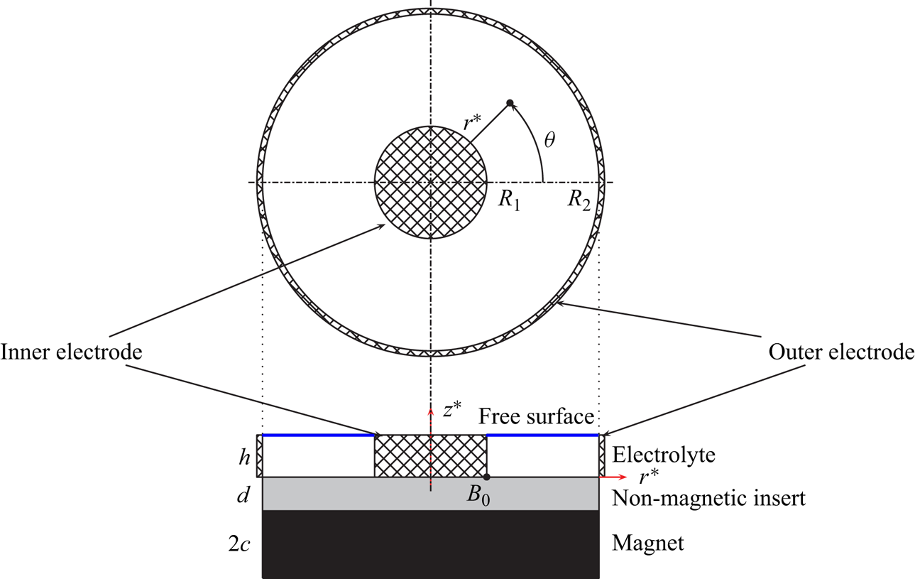
Figure 1. Problem geometry.
Quite unexpectedly, a different type of azimuthally uniform flow referred to as Type 2 solution was also discovered in Suslov et al. (Reference Suslov, Pérez-Barrera and Cuevas2017b). The prominent feature distinguishing it from Type 1 flow is the existence of a secondary counter-rotating toroidal flow structure near the corner formed by the free surface and the outer electrode. Finding this solution came as a surprise because the existence of such a spatially complicated flow structure would generally not be expected in thin layers of viscous fluids. Moreover, the basin of attraction of such a solution has been numerically found to be rather small. Because of that, the convergence of Newton-type iterations to it from a randomly chosen initial guess was literally a ‘lucky’ coincidence. With one such solution found accidentally, the Type 2 solutions for other sets of governing parameters were obtained by using a careful parametric continuation when the solution obtained for one parameter set was used as an initial guess for iterations performed at slightly varied parametric values.
Such a parametric continuation procedure lead to yet another surprise discovery: for a fixed fluid layer depth, Type 2 flow was found to exist only for a finite range of values of the driving electric current or, equivalently, Reynolds numbers (to be defined in § 2)  $Re_{*}\le Re \le Re _{**}$. A further careful investigation undertaken in McCloughan & Suslov (Reference McCloughan and Suslov2020a) revealed that the ways in which Type 2 solution ceases to exist for $Re< Re_{*}$ and $Re>Re_{**}$ are completely different. For small Reynolds numbers, Type 2 solution disappears abruptly via a finite-amplitude ‘jump’ towards Type 1 flow that continues to exist down to $Re=0$ when the driving electric current is switched off and the motion stops. In contrast, in McCloughan & Suslov (Reference McCloughan and Suslov2020a) we established that both Type 1 and 2 flows cease to exist at $Re_{**}$ as a result of a local saddle-node bifurcation when these two solutions ‘collide’ (that is become topologically indistinguishable) and annihilate each other with no other steady azimuthally uniform solution found numerically beyond $Re_{**}$. This posed a question: what happens to a physical flow for large driving currents, that is, for $Re>Re_{**}$?
The experimental observations reported in Pérez-Barrera et al. (Reference Pérez-Barrera, Pérez-Espinoza, Ortiz, Ramos and Cuevas2015, Reference Pérez-Barrera, Ortiz and Cuevas2016), Suslov et al. (Reference Suslov, Pérez-Barrera and Cuevas2017b) and Pérez-Barrera et al. (Reference Pérez-Barrera, Ramírez-Zúñiga, Grespan, Cuevas and del Río2019) provide several hints. First, the circumferential/toroidal flow persists. Second, experiments confirm the existence of a secondary toroidal structure similar to that of Type 2 solution, see figure 17 in Suslov et al. (Reference Suslov, Pérez-Barrera and Cuevas2017b). Third, and most importantly, laboratory observations demonstrated the existence of a robust system of anticyclonic vortices appearing on the free surface of the electrolyte layer (Suslov, Pérez-Barrera & Cuevas Reference Suslov, Pérez-Barrera and Cuevas2017a). Such vortices form an azimuthally propagating periodic structure and thus cannot be attributed to either Type 1 or 2 circumferentially uniform steady solutions. The observations of the flow's temporal evolution also showed that after the driving current is switched on, the circumferential azimuthally invariant flow always establishes first, and only then the vortices appear. This naturally leads to the hypothesis that free-surface vortices result from an instability of an azimuthally uniform steady basic flow, and that they are effectively perturbations superposed on such a basic flow. This led us to perform a linear stability analysis of Type 1 and 2 solutions reported in McCloughan & Suslov (Reference McCloughan and Suslov2020a,Reference McCloughan and Suslovb) for cases when either the Reynolds number or the electrolyte layer depth were varied. It revealed that only Type 2 flows can be unstable with respect to various azimuthally periodic perturbations whereas Type 1 flows are always linearly stable. Therefore, we concluded that the necessary condition for the existence of free-surface vortices is the presence of the secondary toroidal flow structure distinguishing Type 2 solution from its Type 1 counterpart. Our further investigation of the character of such an instability discovered yet another surprising result: while the observable vortices look very much like Kelvin–Helmholtz ‘cat eyes’, Kelvin–Helmholtz instability has nothing to do with their origin. They appear primarily due to Rayleigh's centrifugal instability at the border between two counter-rotating toroidal components of the Type 2 flows.
Since free-surface vortices are observed experimentally even for  $Re>Re_{**}$ (Pérez-Barrera et al. Reference Pérez-Barrera, Pérez-Espinoza, Ortiz, Ramos and Cuevas2015, Reference Pérez-Barrera, Ortiz and Cuevas2016), we hypothesise that they continue to arise on a two-tori background even though the numerical procedure reported in Suslov et al. (Reference Suslov, Pérez-Barrera and Cuevas2017b) and McCloughan & Suslov (Reference McCloughan and Suslov2020a) has failed to find it for large Reynolds numbers. Therefore, our goal here is to make an analytic progress to confirm the existence of a two-tori azimuthally uniform steady flow component beyond the saddle-node bifurcation reported in McCloughan & Suslov (Reference McCloughan and Suslov2020a). We achieve this goal by employing an amplitude expansion procedure specifically designed for regimes that exist a finite parametric distance away from a bifurcation point (Pham & Suslov Reference Pham and Suslov2018). We demonstrate its robustness by using it to develop an asymptotic solution beyond the saddle-node bifurcation and subsequently using it as an initial guess for an iterative search of a full steady solution. We show that the so-initiated iterations converge to a new steady state, which we term Type 3 flow, that is in excellent qualitative and close quantitative agreement with the developed asymptotic approximation. Part 2 of the study then focuses on the stability characteristics of the newly discovered Type 3 flow, compares them with those of the Type 1 and 2 counterparts reported previously and concludes on the roles both Type 2 and Type 3 azimuthally invariant flows play in the formation of experimentally observed free-surface vortices, which are of ultimate interest in various mixing applications.
The structure of Part 1 is as follows. In § 2 we formulate the mathematical problem and specify the appropriate boundary conditions. In § 3, the weakly nonlinear amplitude expansion procedure is developed that aims to approximate solutions at a post-bifurcation point using quantities computed at pre-bifurcation values of the governing parameters. This requires us to deviate from a standard solvability-condition-based derivation of amplitude equations and rigorously justify the variations we introduce to it in order to achieve our goal. In § 4 we discover that the saddle-node bifurcation that leads to the disappearance of Type 1 and 2 solutions is a local feature of a larger-scale fold catastrophe. This enables us to develop an approximate steady-state azimuthally uniform post-bifurcation solution that is different from both Type 1 and 2 solutions but features a prominent two-tori structure satisfying the necessary condition for the existence of experimentally observable free-surface vortices. In § 5 we make further analytical and computational steps and demonstrate that a newly discovered fold catastrophe itself is a part of yet another higher-dimensional (two-parameter) cusp catastrophe. The conclusions are given in § 7, where we also formulate further questions that are answered by a dedicated investigation that is reported in Part 2 of this work.
2. Problem formulation and governing equations
We consider an annular layer of an electrolyte of depth  $h$ laterally confined by vertical coaxial cylindrical electrodes located at $r^*=R_1$ and $r^*=R_2$ (asterisk denotes dimensional quantities), see figure 1. The electrically non-conducting stationary bottom of a container is placed on top of a vertically polarised disc magnet of radius $R_2$ that produces magnetic field $B_0$ at the reference location marked by the black dot in figure 1. The top of the layer is assumed to be stress-free.
The magnetic field created by a permanent magnet is assumed to be axisymmetric. In general, it has both vertical and radial components that vary with horizontal and vertical coordinates:  $\boldsymbol {B}^*=[B_r^*(r^*,z^*),0,B_z^*(r^*,z^*)]$. The magnetic field configuration and details of its computation were discussed in Suslov et al. (Reference Suslov, Pérez-Barrera and Cuevas2017b), see figure 4 in § 4 there. When the electric potential difference ${\rm \Delta} \phi _0$ is applied between the electrodes, the total current
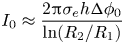 \begin{equation} I_0\approx\frac{2{\rm \pi}\sigma_eh{\rm \Delta}\phi_0}{\ln(R_2/R_1)}\end{equation}
flows mostly radially (see figure 2c) through the layer between them. The interaction of the current and the applied magnetic field creates a Lorentz force  $\boldsymbol {F}_L^*=\boldsymbol {j}^*\times \boldsymbol {B}^*$, where $\boldsymbol {j}^*$ is the current density. This force drives the flow predominantly circumferentially.
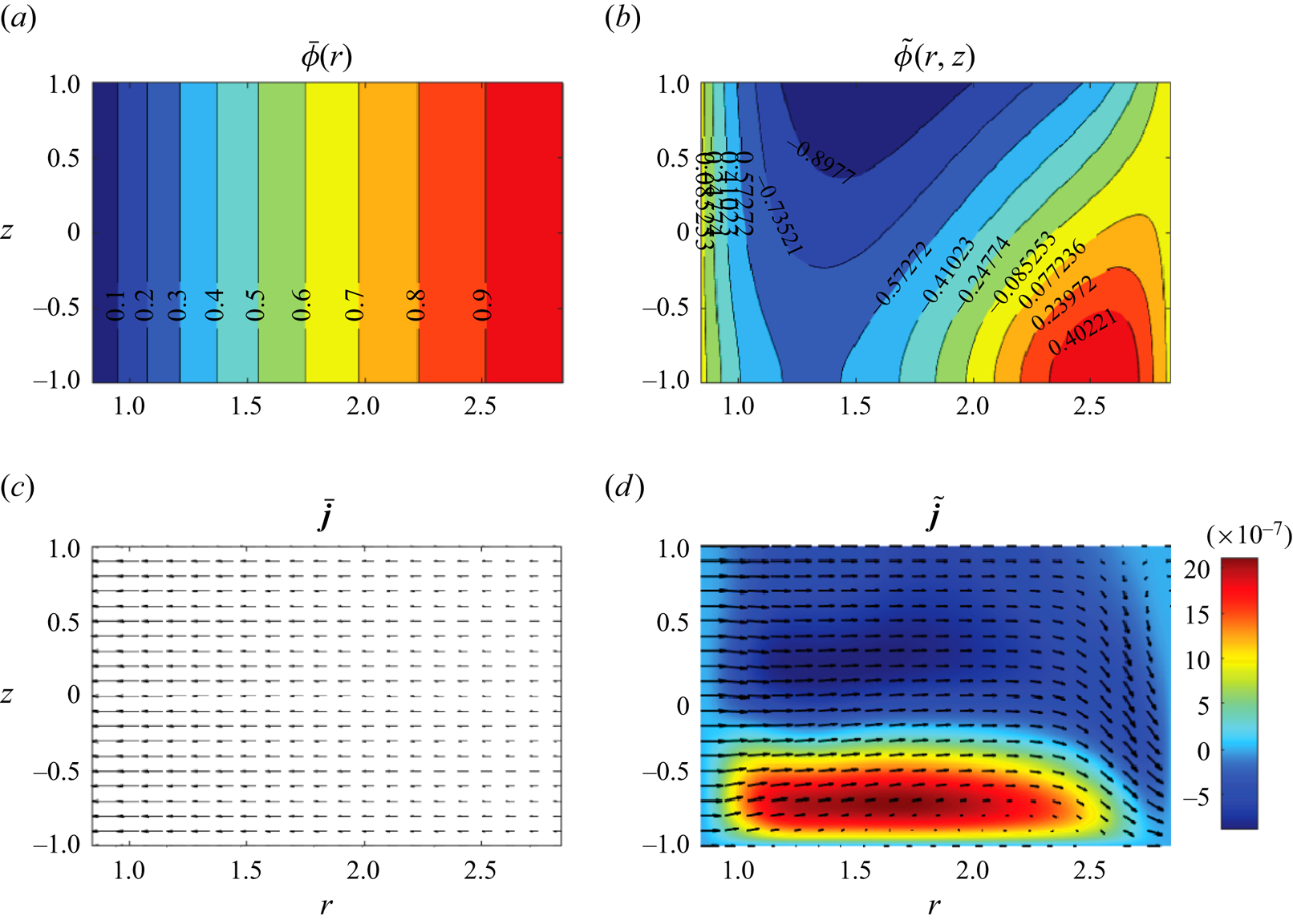
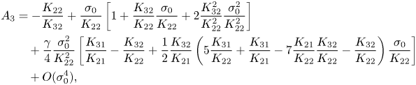
Figure 2. Steady azimuthally invariant distributions of the externally applied (a) and fluid-motion-induced(b) components of the electric potential given by (2.18) and the current components given by (2.21) (c) and (2.22) (b), respectively, for the Type 2 flow at  $(Re,\epsilon )=(1493.88,0.248)$ and $\epsilon ^2{{{Ha}}}^2=1.59\times 10^{-6}$. The colour in the bottom right panel represents the value of the azimuthal electric current component induced by fluid motion.
Because of a low conductivity of electrolytes (see Pérez-Barrera et al. (Reference Pérez-Barrera, Ortiz and Cuevas2016) and Suslov et al. (Reference Suslov, Pérez-Barrera and Cuevas2017b) for typical physical characteristics of an electrolyte), hydrodynamic flows arising in the considered set-up practically do not influence the magnetic field of a magnet and the so-called small magnetic Reynolds number approximation (Davidson Reference Davidson2001) to the equations describing fluid motion can be used. Non-dimensional axisymmetric Poisson's equation for the electric potential, the momentum equations and the continuity equation for an incompressible fluid are then written in cylindrical coordinates as
 $$\begin{gather} {\partial}_{zz}\phi+\epsilon^2\left[{\partial}_{rr}\phi+\dfrac{{\partial}_r\phi }{r}\right]= \epsilon^2 Ha ^2\left[B_r\left(\frac{\epsilon^2 {\partial}_\theta w}{r}-{\partial}_zv\right)+B_z \left({\partial}_rv+\dfrac{v}{r}\right)\right], \end{gather}$$
 $$\begin{gather}{\partial}_tu+u{\partial}_ru-\frac{v^2}{r}+w{\partial}_z u={-}{\partial}_rp+\frac{j_\theta B_z}{\epsilon^2Re} +\frac{1}{Re}\left[{\partial}_{rr}u+\frac{{\partial}_ru}{r}-\frac{u}{r^2} +\frac{{\partial}_{zz}u}{\epsilon^2}\right], \end{gather}$$
 $$\begin{gather}{\partial}_tv+u{\partial}_rv+\frac{uv}{r}+w{\partial}_zv=\frac{j_zB_r-j_rB_z}{\epsilon^2Re} +\frac{1}{Re}\left[{\partial}_{rr}v+\frac{{\partial}_rv }{r}-\frac{v}{r^2}+\frac{{\partial}_{zz} v}{\epsilon^2}\right], \end{gather}$$
 $$\begin{gather}{\partial}_tw+u{\partial} _rw+w{\partial}_zw={-}\frac{{\partial}_zp}{\epsilon^2}-\frac{j_\theta B_r}{\epsilon^2Re} +\frac{1}{Re}\left[{\partial}_{rr}w+\frac{{\partial} _rw}{r}+\frac{{\partial}_{zz}w}{\epsilon^2}\right], \end{gather}$$
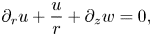 $$\begin{gather}{\partial}_ru+\frac{u}{r}+{\partial}_zw=0, \end{gather}$$
where  $\phi$ is the electric potential, $(u,v,w)$ are the velocity components in the radial ( $r$), azimuthal ( $\theta$) and vertical ( $z$) directions, respectively, and $p$ is the pressure including the hydrostatic component. In the above equations, the non-dimensional magnetic field created by a disc magnet is $\boldsymbol {B}=(B_r,0,B_z)$. The electric current density components are
 \begin{align} j_r={-}{\partial}_r\phi+ Ha ^2v B_z,\quad j_\theta={-} Ha ^2(uB_z-\epsilon^2wB_r),\quad j_z={-}{\partial}_z\phi-\epsilon^2 Ha ^2v B_r.\end{align}
Equations (2.2)–(2.7a–c) are non-dimensionalised as
 \begin{equation} \left.\begin{gathered} (r^*,z^*)=\frac{R_2-R_1}{2}(r,\epsilon z),\quad (u^*,v^*,w^*)=U_0(u,v,\epsilon w),\\ t^*=\frac{R_2-R_1}{2U_0}t,\quad p^*=\rho U_0^2p,\\ (j_r^*,j_\theta^*,j_z^*)=\frac{2\sigma_e{\rm \Delta}\phi_0}{R_2-R_1} \left(j_r,j_\theta,\frac{1}{\epsilon}j_z\right),\quad (B_r^*,B_\theta^*,B_z^*)=B_0(\epsilon B_r,0,B_z), \end{gathered}\right\} \end{equation}
where star denotes dimensional quantities. Here the aspect ratio of the electrolyte layer  $\epsilon$, the square of Hartmann number $ Ha ^2$ characterising electromagnetic effects and Reynolds number $Re$ quantifying viscous effects are
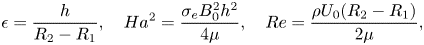 \begin{equation} \epsilon=\frac{h}{R_2-R_1},\quad Ha ^2=\frac{\sigma_eB_0^2h^2}{4\mu},\quad Re=\frac{\rho U_0(R_2-R_1)}{2\mu},\end{equation}
where the velocity scale is defined as  $U_0={\sigma _e{\rm \Delta} \phi _0B_0h^2}/{2\mu (R_2-R_1)}$. The typical experimental values of these parameters are $\epsilon \sim 10^{-1}$, $ Ha ^2\lesssim 10^{-5}$ and $Re\sim 10^3$ (Suslov et al. Reference Suslov, Pérez-Barrera and Cuevas2017b).
The no-slip/no-penetration velocity boundary conditions at the cylindrical electrodes and non-conducting bottom are
 \begin{equation} u=v=w=0 \quad \mbox{at } z={-}1 \quad \mbox{and}\quad \mbox{at } r=\alpha\pm1, \end{equation}
where  $\alpha ={(R_2+R_1)}/{(R_2-R_1)}$ ( $\alpha \approx 1.84$ in experiments described in Pérez-Barrera et al. (Reference Pérez-Barrera, Pérez-Espinoza, Ortiz, Ramos and Cuevas2015) and Suslov et al. (Reference Suslov, Pérez-Barrera and Cuevas2017b) and in our current computations). Neglecting the deformation of the free surface (Satijn et al. Reference Satijn, Cense, Verzicco, Clercx and van Heijst2001; Suslov et al. Reference Suslov, Pérez-Barrera and Cuevas2017b) the tangential stress-free condition is written as
 \begin{equation} w=\partial_zu=\partial_zv=0\quad \mbox{at } z=1. \end{equation}
The boundary conditions for the electric potential at the electrode surfaces, the non-conducting bottom and the free surface are
 $$\begin{gather} \phi=0\mbox{ at }r=\alpha-1\quad \mbox{and}\quad \phi=1\mbox{ at } r=\alpha+1, \end{gather}$$
 $$\begin{gather}{\partial}_z\phi=0\mbox{ at }z={-}1\quad \mbox{and}\quad {\partial}_z\phi={-}\epsilon^2 Ha ^2v B_r\mbox{ at }z=1, \end{gather}$$
respectively.
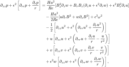
We also note that a steady-state  $\theta$-independent pressure field component satisfies the following Poisson equation (unfortunately, a similar equation given in Suslov et al. (Reference Suslov, Pérez-Barrera and Cuevas2017b) contained a number of unnoticed typesetting errors; it should be replaced with (2.14), with the Froude number multiplying its right-hand side due to a different pressure scaling)
 \begin{align} {\partial}_{zz}p
+\epsilon^2\left[{\partial}_{rr}p+\dfrac{{\partial}_rp}{r}\right]
&=\frac{ Ha ^2}{Re}[B_z^2{\partial}_zw+B_rB_z({\partial}_zu+\epsilon^2{\partial}_rw)+\epsilon^2B_r^2{\partial}_ru] \nonumber\\
&\quad -\frac{ Ha ^2}{2Re}[u{\partial}_rB^2+w{\partial}_zB^2]
+\epsilon^2\omega^2\nonumber\\
&\quad -\frac{1}{2}\left[{\partial}_{zz}u^2+\epsilon^2
\left({\partial}_{rr}u^2+\frac{{\partial}_ru^2}{r}\right)\right] \nonumber\\
&\quad +u\left[{\partial}_{zz}u+\epsilon^2\left({\partial}_{rr}u+\frac{{\partial}_ru}{r}
-\frac{u}{r^2}\right)\right]\nonumber\\
&\quad +v\left[{\partial}_{zz}v+\epsilon^2
\left({\partial}_{rr}v+\frac{{\partial}_rv}{r}-\frac{v}{r^2}\right)\right]\nonumber\\
&\quad +\epsilon^2w\left[{\partial}_{zz}w+\epsilon^2\left({\partial}_{rr}w+
\frac{{\partial}_rw}{r}\right)\right],
\end{align}
\begin{align} {\partial}_{zz}p
+\epsilon^2\left[{\partial}_{rr}p+\dfrac{{\partial}_rp}{r}\right]
&=\frac{ Ha ^2}{Re}[B_z^2{\partial}_zw+B_rB_z({\partial}_zu+\epsilon^2{\partial}_rw)+\epsilon^2B_r^2{\partial}_ru] \nonumber\\
&\quad -\frac{ Ha ^2}{2Re}[u{\partial}_rB^2+w{\partial}_zB^2]
+\epsilon^2\omega^2\nonumber\\
&\quad -\frac{1}{2}\left[{\partial}_{zz}u^2+\epsilon^2
\left({\partial}_{rr}u^2+\frac{{\partial}_ru^2}{r}\right)\right] \nonumber\\
&\quad +u\left[{\partial}_{zz}u+\epsilon^2\left({\partial}_{rr}u+\frac{{\partial}_ru}{r}
-\frac{u}{r^2}\right)\right]\nonumber\\
&\quad +v\left[{\partial}_{zz}v+\epsilon^2
\left({\partial}_{rr}v+\frac{{\partial}_rv}{r}-\frac{v}{r^2}\right)\right]\nonumber\\
&\quad +\epsilon^2w\left[{\partial}_{zz}w+\epsilon^2\left({\partial}_{rr}w+
\frac{{\partial}_rw}{r}\right)\right],
\end{align}
where  $\omega ^2=\omega _r^2+\omega _\theta ^2+\omega _z^2$, $u^2=u^2+v^2+\epsilon ^2w^2$ and $B^2=\epsilon ^2B_r^2+B_z^2$ are squares of the non-dimensional flow vorticity and velocity and of the applied magnetic field. The pressure must satisfy the following boundary conditions
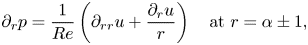 $$\begin{gather} {\partial}_rp =\frac{1}{Re}\left({\partial}_{rr}u+\frac{{\partial}_ru }{r}\right)\quad\mbox{at}\ r=\alpha\pm1, \end{gather}$$
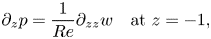 $$\begin{gather}{\partial}_zp =\frac{1}{Re}{\partial}_{zz}w\quad\mbox{at}\ z={-}1, \end{gather}$$
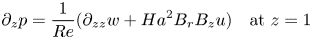 $$\begin{gather}{\partial}_zp =\frac{1}{Re}({\partial}_{zz}w+ Ha ^2B_rB_zu) \quad\mbox{at}\ z=1 \end{gather}$$
that are consistent with the momentum equations in the vicinity of the physical boundaries and take into account the velocity boundary conditions (2.10) and (2.11).
These equations with the specified boundary conditions admit steady  $\theta$-independent solutions (referred to as Type 1 and 2 solutions) that have been discussed in detail in Suslov et al. (Reference Suslov, Pérez-Barrera and Cuevas2017b) and briefly outlined in the introduction here. Linear stability of such solutions with respect to the $m$-periodic infinitesimal perturbations in the form $\boldsymbol {w}'(r,z)\exp ({\sigma t+\textrm {i} m\theta })$ has been subsequently investigated in McCloughan & Suslov (Reference McCloughan and Suslov2020a). Note that the solution of Poisson's equation (2.2) for electric potential with boundary conditions (2.12a,b) and (2.13a,b) can be written as
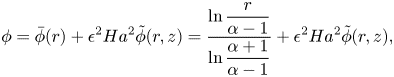 \begin{equation} \phi=\bar\phi(r)+\epsilon^2 Ha ^2\tilde{\phi}(r,z) =\frac{\ln\dfrac{r}{\alpha-1}}{\ln\dfrac{\alpha+1}{\alpha-1}} +\epsilon^2 Ha ^2\tilde{\phi}(r,z),\end{equation}
where
 $$\begin{gather} \tilde{\phi}=0\quad\mbox{at}\ r=\alpha-1\quad\mbox{and}\quad r=\alpha+1, \end{gather}$$
 $$\begin{gather}{\partial}_z\tilde{\phi}=0\quad\mbox{at}\ z={-}1\quad\mbox{and}\quad {\partial}_z\tilde{\phi}={-}vB_r\quad\mbox{at}\ z=1. \end{gather}$$
This potential induces the electric current  $\boldsymbol {j}=\bar{\boldsymbol{j}}+\tilde{\boldsymbol{j}}$, where
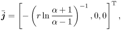 $$\begin{gather} \bar{\boldsymbol{j}} = \left[-\left(r\ln\frac{\alpha+1}{\alpha-1}\right)^{{-}1},0,0\right]^{\rm T}, \end{gather}$$
 $$\begin{gather}\tilde{\boldsymbol{j}} = Ha ^2[vB_z-\epsilon^2{\partial}_r\tilde{\phi}, \epsilon^2wB_r-uB_z,-\epsilon^2({\partial}_z\tilde{\phi}+vB_r)]^{\rm T}. \end{gather}$$
The example of such steady azimuthally invariant electric potential and current distributions is shown in figure 2. It demonstrates that the maximum variation of the electric potential across the flow domain induced by a steady fluid motion field  ${\bar{\boldsymbol{u}}=[\bar u(r,z),\bar v(r,z),\bar w(r,z)]^\textrm {T}}$ does not exceed $1.5\times 10^{-4}\%$ of the applied electric potential difference so that the associated variation of the Lorentz force remains negligible. The induced current tends to reduce the total (predominantly radial) current, but quantitatively such a reduction is negligible compared with the current applied externally. In view of this, in what follows we neglect any time-dependent perturbations $\phi '(r,z,t)$ of the steady-state potential $\bar \phi +\tilde {\phi }$ that could be induced by an unsteady velocity field perturbations $|\boldsymbol {u}'(r,z,t)|\ll |\bar{\boldsymbol{u}}(r,z)|$. This reduces the system of perturbation equations and the corresponding computational cost. A systematic relative error $|\phi '|/|\boldsymbol {u}'|$ introduced by neglecting $\phi '$ in the linearised equations discussed in the following is of the order of $\epsilon ^2 Ha ^2\sim 10^{-6}$ that we deem acceptable compared with the error of the order of $10^{-4}$ introduced by truncating the asymptotic series developed in § 3. The resulting linearised perturbation equations have been given explicitly in McCloughan & Suslov (Reference McCloughan and Suslov2020a) and will not be repeated here. We just mention for the future reference that they can be written in an operator form as
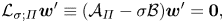 \begin{equation} \mathcal{L}_{\sigma;\varPi}\boldsymbol{w}'\equiv(\mathcal{A}_\varPi-\sigma\mathcal{B})\boldsymbol{w}'=\boldsymbol{0},\end{equation}
where  $\sigma =\sigma ^R+\textrm {i}\sigma ^I$ is the complex amplification rate and $\mathcal {L}_{\sigma ;\varPi }$, $\mathcal {A}_\varPi$ and $\mathcal {B}$ are matrix-differential and matrix operators, respectively, arising from the linearised perturbation equations and boundary conditions,
 \begin{equation} \boldsymbol{w}'=[u'(r,z),v'(r,z),u'_z(r,z), p'(r,z)]^{\rm T} \end{equation}
is the vector of meridional perturbation quantities,  $\varPi =\{Re,\epsilon,m\}$ is the set of the governing parameters. Hartmann number is fixed to zero in stability equations. In the subsequent analysis we also take $m=0$ so that only $\theta$-independent component of the flow is considered.
3. Weakly nonlinear formulation
Solutions of linearised equations (2.23) for various values of the governing parameters  $\varPi$ are eigenfunctions corresponding to a discrete eigenvalue spectrum $\sigma _i$. The eigenvalues are sorted in the order of a decreasing real part
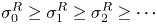 \begin{equation} \sigma_0^R\geq\sigma_1^R \geq \sigma_2^R \geq\cdots \end{equation}
and only eigenfunctions corresponding to  $\sigma _i^R>0$, $i=0,1,2,\ldots$ (temporally growing perturbations) are deemed to represent physically observable flow patterns. For Type 1 and 2 basic flows, they have been discussed in detail in McCloughan & Suslov (Reference McCloughan and Suslov2020a), where it was shown computationally that at most one unstable eigenfunction can be identified for each set of the governing parameters. Furthermore, it was also established in McCloughan & Suslov (Reference McCloughan and Suslov2020a) that Type 1 basic flow remained linearly stable whereas Type 2 solutions were unstable with respect to perturbations with wavenumbers $m$ belonging to a finite range. Importantly, it was demonstrated that azimuthally invariant perturbations with $m=0$ grew most rapidly. This prompted their weakly nonlinear consideration that was carried out up to the second order in perturbation amplitude, which enabled the authors to conclude that Type 1 and 2 solutions undergo a local saddle-node bifurcation at $Re=Re_{**}$. Here we extend that study to include third-order terms so that we can understand global dynamics of the considered physical system beyond the bifurcation point and discover a hierarchy of catastrophes experienced by the flow as its governing parameters change. The same Chebyshev pseudo-spectral collocation method was used as that described in Suslov et al. (Reference Suslov, Pérez-Barrera and Cuevas2017b) and McCloughan & Suslov (Reference McCloughan and Suslov2020a). Further details of the numerical implementation will be presented in Part 2 of this paper.
Let  $\bar {\boldsymbol {w}}$ represent the steady $\theta$-invariant basic flow solution vector computed at $Re_0\lesssim Re _{**}$ ( $Re_0$ cannot be exactly equal to or greater than $Re_{**}$ because both the Type 1 and 2 solutions cease to exist and the computational procedure fails to converge there). As discussed in McCloughan & Suslov (Reference McCloughan and Suslov2020a) the generalised eigenvalue problem (2.23) derived for $m=0$ from equations linearised about $\bar {\boldsymbol {w}}$ results in a real growth rate $\sigma _0=\sigma _0^R$, which tends to zero at $Re_0\to Re _{**}$. The corresponding eigenfunction is defined up to an arbitrary multiplicative amplitude $A$. Since the maximum perturbation growth rate is close to zero, the magnitude of the amplitude must be small. Therefore, we rescale it by introducing a formal order parameter $\zeta$: $A=\zeta \tilde {A}$, where $\tilde {A}=O(1)$. We also introduce the scaled parametric distance from point $Re_0$: $\delta =\zeta ^2\tilde {\delta }=(Re-Re_0)/Re_0$, $\tilde {\delta }=O(1)$.
We look for the asymptotic solution in the vicinity of  $Re_0$ in the form that is informed by the fact that the governing equations have a quadratic nonlinearity (e.g. Pham & Suslov Reference Pham and Suslov2018):
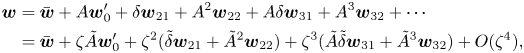 \begin{align} \boldsymbol{w} &= \bar{\boldsymbol{w}}+A\boldsymbol{w}'_0+\delta\boldsymbol{w}_{21}+A^2\boldsymbol{w}_{22}+A\delta\boldsymbol{w}_{31}+A^3\boldsymbol{w}_{32}+\cdots \nonumber\\ &= \bar{\boldsymbol{w}}+\zeta\tilde{A}\boldsymbol{w}'_0+\zeta^2(\tilde{\delta}\boldsymbol{w}_{21}+\tilde{A}^2\boldsymbol{w}_{22})+ \zeta^3(\tilde{A}\tilde{\delta}\boldsymbol{w}_{31}+\tilde{A}^3\boldsymbol{w}_{32})+O(\zeta^4), \end{align}
where the vector of flow quantities is  $\boldsymbol {w}=[u,v,w,p]^\textrm {T}$. Subscripts 21, 31 and 22, 32 denote flow deviations from $\bar {\boldsymbol {w}}$ computed for $Re_0$ due to the variation of the governing parameter ( $Re\ne Re _0$) and contributions due to the nonlinearity of the problem, respectively.
Substituting (3.2) into the governing equations (2.3)–(2.7a–c) and boundary conditions (2.10) and (2.11) we regain the basic flow equations from the  $\zeta ^0$ terms and the linearised perturbation equations at the order of $\zeta ^1$, that is,
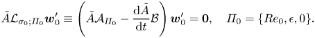 \begin{equation} \tilde{A}\mathcal{L}_{\sigma_0;\varPi_0}\boldsymbol{w}_0'\equiv\left(\tilde{A}\mathcal{A}_{\varPi_0}- \frac{{\rm d}\tilde{A}}{{\rm d} t}\mathcal{B}\right)\boldsymbol{w}_0'=\boldsymbol{0},\quad {\varPi_0=\{Re_0,\epsilon,0\}}.\end{equation}
It follows from comparing (2.23) and (3.3) that
 \begin{equation} \frac{{\rm d} \tilde{A}}{{\rm d} t}=\sigma_0\tilde{A}\end{equation}
and that  $\mathcal {L}_{\sigma _0;\varPi _0}$ is necessarily a singular operator, which is required to obtain a non-trivial perturbation solution $\boldsymbol {w}'_0$.
Equations arising at the second order of  $\zeta$ can be written as
 \begin{align} \tilde{\delta}\mathcal{A}_{0;\varPi_0}\boldsymbol{w}_{21}+\left(\tilde{A}^2\mathcal{A}_{\varPi_0}-\frac{{\rm d}\tilde{A}^2}{{\rm d} t}\mathcal{B}\right)\boldsymbol{w}_{22} \equiv\tilde{\delta}\mathcal{L}_{0;\varPi_0}\boldsymbol{w}_{21}+\tilde{A}^2\mathcal{L}_{2\sigma_0;\varPi_0}\boldsymbol{w}_{22} =\tilde{\delta}\boldsymbol{f}_{21}+\tilde{A}^2\boldsymbol{f}_{22}, \end{align}
since in view of (3.4)
 \begin{equation} \frac{{\rm d}\tilde{A}^2}{{\rm d} t}=2\sigma_0\tilde{A}^2, \end{equation}
where  $\boldsymbol {f}_{21}=[f_{21}^{(1)}\ f_{21}^{(2)}\ f_{21}^{(3)}\ 0]^\textrm {T}$ and $\boldsymbol {f}_{22}=[f_{22}^{(1)}\ f_{22}^{(2)}\ f_{22}^{(3)}\ 0]^\textrm {T}$ are defined in Appendix A. Equation (3.5) is equivalent to a system of two-component equations
 \begin{equation} \mathcal{L}_{0;\varPi_0}\boldsymbol{w}_{21}=\boldsymbol{f}_{21}\quad \mbox{and}\quad \mathcal{L}_{2\sigma_0;\varPi_0}\boldsymbol{w}_{22}=\boldsymbol{f}_{22}. \end{equation}
The operators in the left-hand sides of these equations are not singular and, thus, (3.7a,b) can be solved uniquely. However, since the computational parametric point  $\varPi _0$ is arbitrarily chosen in the vicinity of $\varPi _{**}=\{Re_{**},\epsilon,0\}$, it can approach it asymptotically closely. In this limit, $\sigma _0\to 0$ and the operators in the left-hand sides of (3.7a,b) become singular. Therefore, the existence of solutions of these equations with non-zero right-hand sides cannot be guaranteed unless the right-hand-side vectors are put in the range of the operators. The additional degree of freedom required for adjusting the right-hand sides is obtained by noting that (3.4) describing a fast exponential evolution is only valid for an infinitesimal amplitude and it must be modified whenever the amplitude acquires a finite size. Algebraically, this is done by adding terms to the evolution equation (3.4) that have functional forms identical to those of terms appearing in the amplitude expansion (3.2) at any particular order. Therefore, we write
 \begin{equation} \frac{{\rm d}\tilde{A}}{{\rm d} t}=\sigma_0\tilde{A}+\zeta(K_{12}\tilde{\delta}+K_{22}\tilde{A}^2),\end{equation}
which leads to the appearance of additional terms in (3.7a,b):
 \begin{equation} \mathcal{L}_{0;\varPi_0}\boldsymbol{w}_{21}=\boldsymbol{f}_{21}+K_{21}\mathcal{B}\boldsymbol{w}'_0,\quad \mathcal{L}_{2\sigma_0;\varPi_0}\boldsymbol{w}_{22}=\boldsymbol{f}_{22}+K_{22}\mathcal{B}\boldsymbol{w}'_0.\end{equation}
Taking the limit of  $\varPi _0\to \varPi _{**}$ or, equivalently, $\sigma _0\to 0$, $\boldsymbol {w}'_0\to \boldsymbol {w}'_{**}$, which makes the operators in the left-hand side of (3.9a,b) identical and singular, and considering the inner product of these equations with the adjoint eigenvector $\boldsymbol {w}_{**}^{\dagger}$ of $\mathcal {L}_{0;\varPi _{**}}$ normalised as $\langle \boldsymbol {w}_{**}^{\dagger},\mathcal {B}\boldsymbol {w}'_ {**}\rangle =1$ we obtain the classical solvability conditions that define constants $K_{21}$ and $K_{22}$ (Landau Reference Landau1944; Stuart Reference Stuart1960; Watson Reference Watson1960)
 \begin{equation} 0=\langle\boldsymbol{w}_{**}^{\dagger},\boldsymbol{f}_{21}\rangle+K_{21},\quad 0=\langle\boldsymbol{w}_{**}^{\dagger},\boldsymbol{f}_{22}\rangle+K_{22}.\end{equation}
However, implementing the above in practice in the current problem is impossible because neither steady-state basic flow solutions, nor their linearised perturbation, nor the adjoint eigenvector can be found at  $\varPi _{**}$ (see also the discussion in McCloughan & Suslov Reference McCloughan and Suslov2020a). This means that all computations necessarily have to be performed at $\varPi _0\ne \varPi _{**}$ so that $\sigma _0\ne 0$ and the operators in the left-hand sides of (3.9a,b) remain non-singular, thus, making the choice of $K_{21}$ and $K_{22}$ ambiguous (given that for non-singular left-hand sides these equations can be solved for any values of the constants). As was explained in Pham & Suslov (Reference Pham and Suslov2018) such an ambiguity is not an algebraic artefact but rather is a reflection of physical reality: away from the critical point one must chose explicitly the angle of the desired projection of the full solution of the physical problem onto a space spanned by the eigenfunctions of the linearised perturbation problem. In other words, this means that one has to provide an additional condition specifying the main features of the physical problem that are to be retained as closely as possible under the solution projection given by (3.2). As algorithmically proven in Pham & Suslov (Reference Pham and Suslov2018) and discussed previously in Suslov & Paolucci (Reference Suslov and Paolucci1997, Reference Suslov and Paolucci1999) and references therein this additional requirement is formulated as the weighted orthogonality conditions
 \begin{equation} 0=\langle\boldsymbol{w}_{21},\mathcal{M}\boldsymbol{w}'_0\rangle,\quad 0=\langle\boldsymbol{w}_{22},\mathcal{M}\boldsymbol{w}'_0\rangle,\end{equation}
where  $\mathcal {M}$ is an appropriate weight matrix. Here we choose
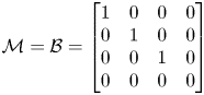 \begin{equation} \mathcal{M}=\mathcal{B}=\left[\begin{array}{@{}cccc@{}} 1 & 0 & 0 & 0\\ 0 & 1 & 0 & 0\\ 0 & 0 & 1 & 0\\ 0 & 0 & 0 & 0 \end{array}\right] \end{equation}
so that the higher-order terms in (3.2) are weight-orthogonal to the eigenfunctions of the linearised perturbation problem and the low-order truncation of this asymptotic series retains most of the kinetic energy of the full nonlinear solution of the original problem. Subsequently, as shown in Pham & Suslov (Reference Pham and Suslov2018) equations (3.9a,b) are recast as extended systems
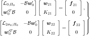 \begin{equation} \left.\begin{gathered} \left[\begin{array}{@{}cc@{}} \mathcal{L}_{0;\varPi_0} & -\mathcal{B}\boldsymbol{w}_0'\\ \boldsymbol{w}_0^{\prime T}\mathcal{B} & 0 \end{array}\right] \left[\begin{array}{c} \boldsymbol{w}_{21}\\ K_{21} \end{array}\right]= \left[\begin{array}{c} \boldsymbol{f}_{21}\\ 0 \end{array}\right],\\ \left[\begin{array}{@{}cc@{}} \mathcal{L}_{2\sigma_0;\varPi_0} & -\mathcal{B}\boldsymbol{w}_0'\\ \boldsymbol{w}_0^{\prime T}\mathcal{B} & 0 \end{array}\right] \left[\begin{array}{c} \boldsymbol{w}_{22}\\ K_{22} \end{array}\right] =\left[\begin{array}{c} \boldsymbol{f}_{22}\\ 0 \end{array}\right] \end{gathered}\right\} \end{equation}
that are proven to be non-singular and, thus, can be solved using any standard computational routine for systems of linear equations to simultaneously define  $(\boldsymbol {w}_{21},K_{21})$ and $(\boldsymbol {w}_{22},K_{22})$.
Proceeding similarly with equations arising at the third order of  $\zeta$ and taking into account that
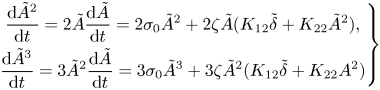 \begin{equation} \left.\begin{gathered} \frac{{\rm d}\tilde{A}^2}{{\rm d} t}=2\tilde{A}\frac{{\rm d}\tilde{A}}{{\rm d} t}=2\sigma_0\tilde{A}^2 +2\zeta\tilde{A}(K_{12}\tilde{\delta}+K_{22}\tilde{A}^2),\\ \frac{{\rm d}\tilde{A}^3}{{\rm d} t}=3\tilde{A}^2\frac{{\rm d}\tilde{A}}{{\rm d} t}=3\sigma_0\tilde{A}^3 +3\zeta\tilde{A}^2(K_{12}\tilde{\delta}+K_{22}A^2) \end{gathered}\right\} \end{equation}
we obtain
 \begin{equation} \frac{{\rm d}\tilde{A}}{{\rm d} t}=\sigma_0\tilde{A}+\zeta(K_{21}\tilde{\delta}+K_{22}\tilde{A}^2) +\zeta^2(K_{31}\tilde{A}\tilde{\delta}+K_{32}\tilde{A}^3)\end{equation}
and
 \begin{equation} \tilde{A}\tilde{\delta}\mathcal{L}_{\sigma_0;\varPi_0}\boldsymbol{w}_{31}+\tilde{A}^3\mathcal{L}_{3\sigma_0;\varPi_0}\boldsymbol{w}_{32} =\tilde{A}\tilde{\delta} (K_{31}\mathcal{B}\boldsymbol{w}'+\boldsymbol{f}_{31})+\tilde{A}^3(K_{32}\mathcal{B}\boldsymbol{w}'+\boldsymbol{f}_{32}),\end{equation}
where  $\boldsymbol {f}_{31}=[f_{31}^{(1)}\ f_{31}^{(2)}\ f_{31}^{(3)}\ 0]^\textrm {T}$ and $\boldsymbol {f}_{32}=[f_{32}^{(1)}\ f_{32}^{(2)}\ f_{32}^{(3)}\ 0]^\textrm {T}$ are defined in Appendix A. Then $(\boldsymbol {w}_{31},K_{31})$ and $(\boldsymbol {w}_{32},K_{32})$ are found from
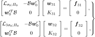 \begin{equation} \left.\begin{gathered} \left[\begin{array}{@{}cc@{}} \mathcal{L}_{\sigma_0;\varPi_0} & -\mathcal{B}\boldsymbol{w}_0'\\ \boldsymbol{w}_0^{\prime T}\mathcal{B} & 0 \end{array}\right] \left[\begin{array}{c} \boldsymbol{w}_{31}\\ K_{31} \end{array}\right] =\left[\begin{array}{c} \boldsymbol{f}_{31}\\ 0 \end{array}\right],\\ \left[\begin{array}{@{}cc@{}} \mathcal{L}_{3\sigma_0;\varPi_0} & -\mathcal{B}\boldsymbol{w}_0'\\ \boldsymbol{w}_0^{\prime T}\mathcal{B} & 0 \end{array}\right] \left[\begin{array}{c} \boldsymbol{w}_{32}\\ K_{32} \end{array}\right] =\left[\begin{array}{c} \boldsymbol{f}_{32}\\ 0 \end{array}\right], \end{gathered}\right\} \end{equation}
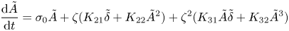
respectively. Finally, rewriting  $\tilde {A}$ and $\tilde {\delta }$ in terms of $A$ and $\delta$ in (3.15) leads to the amplitude equation
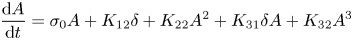 \begin{equation} \frac{{\rm d} A}{{\rm d} t}=\sigma_0A+K_{12}\delta+K_{22}A^2+K_{31}\delta A+K_{32}A^3 \end{equation}
governing the temporal evolution of the  $\theta$-independent flow component near $\varPi _0$.
4. Fold catastrophe
4.1. Determining fold points
The cubic amplitude equation (3.18) with real coefficients can have either one or three real fixed points, see figure 3(a). Of interest here is the parameter set, where the number of such points changes, that is, the fold catastrophe. In terms of parameters defined in the previous sections, the task is to estimate  $Re_{**}$ at which the Type 1 and 2 steady $\theta$-independent solutions cease to exist given (3.18) with coefficients estimated at $Re_0< Re_{**}$. This is required since direct computations at $Re_{**}$ are impossible, see figure 3(b), where a closeup of a fold is shown. The circles show the closest location to the catastrophe at which computing the two distinct steady $\theta$-independent basic flow solutions is still possible. The phase diagram in figure 3(b) is topologically equivalent to that discussed in detail in McCloughan & Suslov (Reference McCloughan and Suslov2020a). Therefore, we conclude that the saddle-node bifurcation analysed there is just a local feature of a larger-scale fold catastrophe that we discovered here by considering a higher-order amplitude expansion of the flow fields.
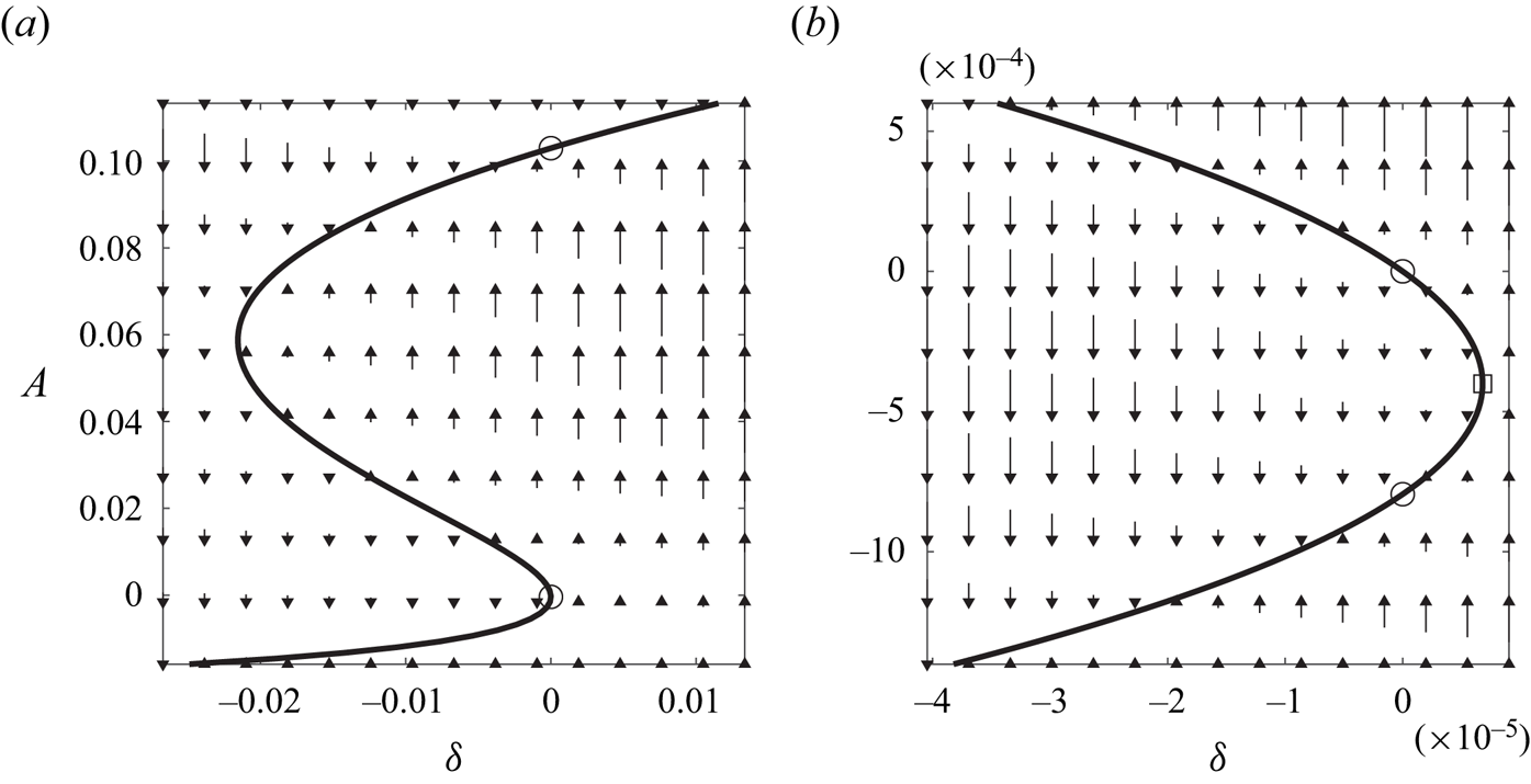
Figure 3. (a) Fold catastrophe and (b) saddle-node bifurcation phase diagrams computed for the Type 2 basic flow at  $\varPi _0=(Re_0,\epsilon, Ha ,m)=(1493.88,0.248,5.08\times 10^{-3},0)$. The curves show the location of fixed points of (3.18) and the vectors correspond to the value of ${\textrm {d} A}/{\textrm {d} t}$. The circles indicate values of the fixed-point amplitudes at $\delta =0$ corresponding to the computational parametric point $\varPi _0$ and the square marks the position of the predicted fold catastrophe point that is not accessible by direct computations.
Setting  ${\textrm {d} A}/{\textrm {d} t}=0$ in (3.18), differentiating it with respect to $A$, taking into account that at the catastrophe point ${\textrm {d}\delta }/{\textrm {d} A}=0$ and solving for $\delta$ we find the location of the fold catastrophe in terms of $A$:
$A$:
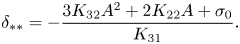 \begin{equation} \delta_{**}={-}\frac{3K_{32}A^2+2K_{22}A+\sigma_0}{K_{31}}. \end{equation}
Substituting  $\delta =\delta _{**}$ from (4.1) to (3.18) leads to a cubic equation for $A$ at the fold catastrophe point:
 \begin{equation} 2K_{31}K_{32}A^3+(K_{22}K_{31}+3K_{21}K_{32})A^2 +2K_{21}K_{22}A+\sigma_0K_{21}=0,\end{equation}
which for  $\sigma _0\to 0$ has an asymptotically small solution
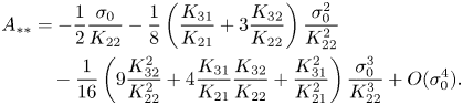 \begin{align} A_{**} &={-}\frac{1}{2}\frac{\sigma_0}{K_{22}}-\frac{1}{8} \left(\frac{K_{31}}{K_{21}}+3\frac{K_{32}}{K_{22}}\right)\frac{\sigma_0^2}{K_{22}^2} \nonumber\\ &\quad -\frac{1}{16}\left(9\frac{K_{32}^2}{K_{22}^2}+4\frac{K_{31}}{K_{21}} \frac{K_{32}}{K_{22}}+\frac{K_{31}^2}{K_{21}^2}\right)\frac{\sigma_0^3}{K_{22}^3} +O(\sigma_0^4). \end{align}
Finally, from (4.1) and (4.3) we obtain the approximate location of the fold catastrophe point
 \begin{align} Re_{**}=Re_0(1+\delta_{**}),\quad \delta_{**}=\frac{\sigma_0^2}{4K_{21}K_{22}} \left[1+\frac{1}{2}\left(\frac{K_{31}}{K_{21}}+\frac{K_{32}}{K_{22}}\right) \frac{\sigma_0}{K_{22}}+O(\sigma_0^2)\right].\end{align}
4.2. Parameter sensitivity considerations
While (4.4a,b) enables one to determine the fold catastrophe point by computing coefficients of the amplitude equation (3.18) at a parametric point  $\varPi _0$ some distance away from it, the question arises how sensitive such a prediction is to the choice of $\varPi _0$. As seen from figure 4(a–e) the coefficients of (3.18) do not remain constant as $Re$ deviates from $Re_{**}$, which is expected since they depend on the structure of both basic flow and perturbation fields that vary with the strength of an electric current that determines the value of $Re$. However, the estimations of $Re_{**}$ remain sufficiently robust, see figure 4( $\,f$). For example, for $Re_0=1493.88$ (the largest value of Reynolds number for which the steady $\theta$-independent basic flow solutions can be computed, see black circles in figure 4) we obtain $Re_{**}=1493.92$, whereas for $Re_0=1470.00$ we compute $Re_{**}=1491.49$. Therefore, shifting the computational point by ${1493.88}/{1470.00}-1\approx 0.016$ leads to the $Re_{**}$ estimation error that is at least an order of magnitude smaller than this shift: ${1493.92}/{1491.49}-1\approx 0.0016$. Thus, the suggested weakly nonlinear expansion procedure enables one to obtain accurate solutions without approaching the catastrophe point asymptotically closely. This is a practically important conclusion: while the solution at $Re_0=1470.00$ can be obtained starting with a relatively crude initial guess, a very careful parametric continuation procedure with at least 50 intermediate computations, each providing an initial guess for the subsequent run, was required to approach the value of $Re_0=1493.88$. This is so because such an approach has to be strictly one-sided with progressively decreasing parametric increments since overshooting $Re_{**}$ completely breaks the catastrophe search process given that for $Re>Re_{**}$ solutions cease to exist and Newton-type iterations cannot converge in principle.
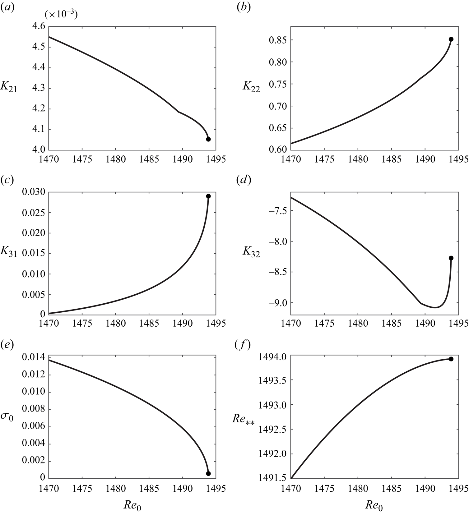
Figure 4. Coefficients of (3.18) evaluated for Type 2 basic flow and estimations of  $Re_{**}$ as functions of $Re_0$ for $(\epsilon, Ha )=(0.248,5.08\times 10^{-3})$. Black circles show the values computed at the parametric point that is closest to the catastrophe point, where convergence of iterations can still be achieved.
4.3. Post-fold catastrophe solution
Once the location of the catastrophe point  $Re_{**}$ is determined, the natural question arises: what happens to the physical flow at larger Reynolds numbers? Since Type 1 and 2 steady $\theta$-independent basic flow solutions cease to exist, multiple scenarios may be considered. One of them is that another steady $\theta$-invariant flow state may exist. However, as reported in Suslov et al. (Reference Suslov, Pérez-Barrera and Cuevas2017b) and McCloughan & Suslov (Reference McCloughan and Suslov2020a), attempts to find the third solution directly using Newton-type iterations, similarly to how Type 1 and 2 basic flows were found, fail. This indicates that even if such a solution does exist, its basin of attraction is sufficiently far from solutions found previously. Thus, we resort to the analysis of the third fixed point of (3.18) that belongs to the upper branch of the S-shaped curve in figure 3(a), see the top circle there. It exists in the finite neighbourhood of $\varPi _{**}$ for $Re\gtrless Re _{**}$. We denote the value of the amplitude at that point by $A_3$ and find an explicit asymptotic expression for it in the limit $\sigma _0\to 0$ (or, equivalently, $\varPi \to \varPi _{**}$):
 \begin{align} A_3 &={-}\frac{K_{22}}{K_{32}}+\frac{\sigma_0}{K_{22}} \left[1+\dfrac{K_{32}}{K_{22}}\frac{\sigma_0}{K_{22}} +2\frac{K_{32}^2}{K_{22}^2}\frac{\sigma_0^2}{K_{22}^2}\right] \nonumber\\ &\quad +\frac{\gamma}{4}\frac{\sigma_0^2}{K_{22}^2} \left[\frac{K_{31}}{K_{21}}-\frac{K_{32}}{K_{22}}+\frac{1}{2}\frac{K_{32}}{K_{21}} \left(5\frac{K_{31}}{K_{22}}+\frac{K_{31}}{K_{21}}-7\frac{K_{21}}{K_{22}}\frac{K_{32}}{K_{22}} -\frac{K_{32}}{K_{22}}\right) \frac{\sigma_0}{K_{22}}\right] \nonumber\\ &\quad +O(\sigma_0^4), \end{align}
where  $\gamma ={(Re-Re_0)}/{(Re_{**}-Re_0)}$, $Re$ is the Reynolds number of interest, $Re_0$ is the Reynolds number at which the coefficients of (3.18) are evaluated and $Re_{**}$ is the Reynolds number of the catastrophe point (approximately given by (4.4a,b)). This enables us to reconstruct the corresponding steady azimuthally invariant component of the flow field using (3.2). To do that, we choose $Re_0=1493.88< Re_{**}$ for which we still can find two distinct steady-state solutions by a standard iterative process. It has been shown in McCloughan & Suslov (Reference McCloughan and Suslov2020a) that both Type 1 and 2 basic flows can be used to determine equally good estimations of the catastrophe point $Re_{**}$. However, since our goal here is to approximate the third steady-state solution that is topologically ‘closer’ to the Type 2 basic flow (corresponding to the middle segment of the S-shaped curve in figure 3a), we use the latter as $\bar {\boldsymbol {w}}$ in (4.4a,b). Subsequently, we compute the coefficients and component fields $\boldsymbol {w}'$, $\boldsymbol {w}_{21}$, $\boldsymbol {w}_{22}$, $\boldsymbol {w}_{31}$ and $\boldsymbol {w}_{32}$. The coefficient values that we obtain using $N_r\times N_z=51\times 40$ spectral collocation modes (rather than $N_r\times N_z=45\times 31$ used in Suslov et al. (Reference Suslov, Pérez-Barrera and Cuevas2017b) and McCloughan & Suslov (Reference McCloughan and Suslov2020a), where the details of numerical approximation have been given) are listed in table 1. Note that the $\sigma _0$, $K_{21}$ and $K_{22}$ values reported here are somewhat different from those reported previously in McCloughan & Suslov (Reference McCloughan and Suslov2020a). This is partially because of a higher spatial resolution used to produce the current results as well as because of the properties of the Matlab (The MathWorks 2020) routine eigs used to compute eigenvectors. It has an internal eigenvector scaling procedure returning results that generally depend on a particular computer architecture so that the same code can return differently scaled eigenvectors when it runs on different computers. Of course, this has no effect on the reported physical results: different scaling of eigenvectors leads to the corresponding change of the computed coefficients and amplitudes so that the product $A\boldsymbol {w}'$ remains invariant and so does the location $Re_{**}\approx 1493.92$ of the catastrophe point.
Table 1. Values of coefficients entering (3.18) and the location of a catastrophe point computed for  $\varPi _0=(Re_0,\epsilon, Ha ) =(1493.88,0.248,5.08\times 10^{-3})$.

This enables us to estimate the value of  $A_3\approx 1.04\times 10^{-1}$ at a representative value of $Re=1500>Re_{**}$ ( $\gamma =153$), see figure 3(a), where we now can reconstruct the post-catastrophe steady $\theta$-independent flow component that cannot be computed directly. Figures 5–8 depict the flow fields for each component of the asymptotic solution and figure 11 shows the approximated full flow field given by (3.2). Panels (a) and (b) in each figure illustrate the meridional velocity and the azimuthal vorticity of the flow field, respectively.
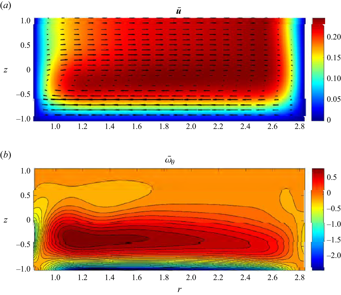
Figure 5. Meridional  $\theta$-independent steady Type 2 basic flow velocity (a) and azimuthal vorticity (b) fields near the fold catastrophe point for $(Re_0,\epsilon, Ha )=(1493.88,0.248,5.08\times 10^{-3})$.
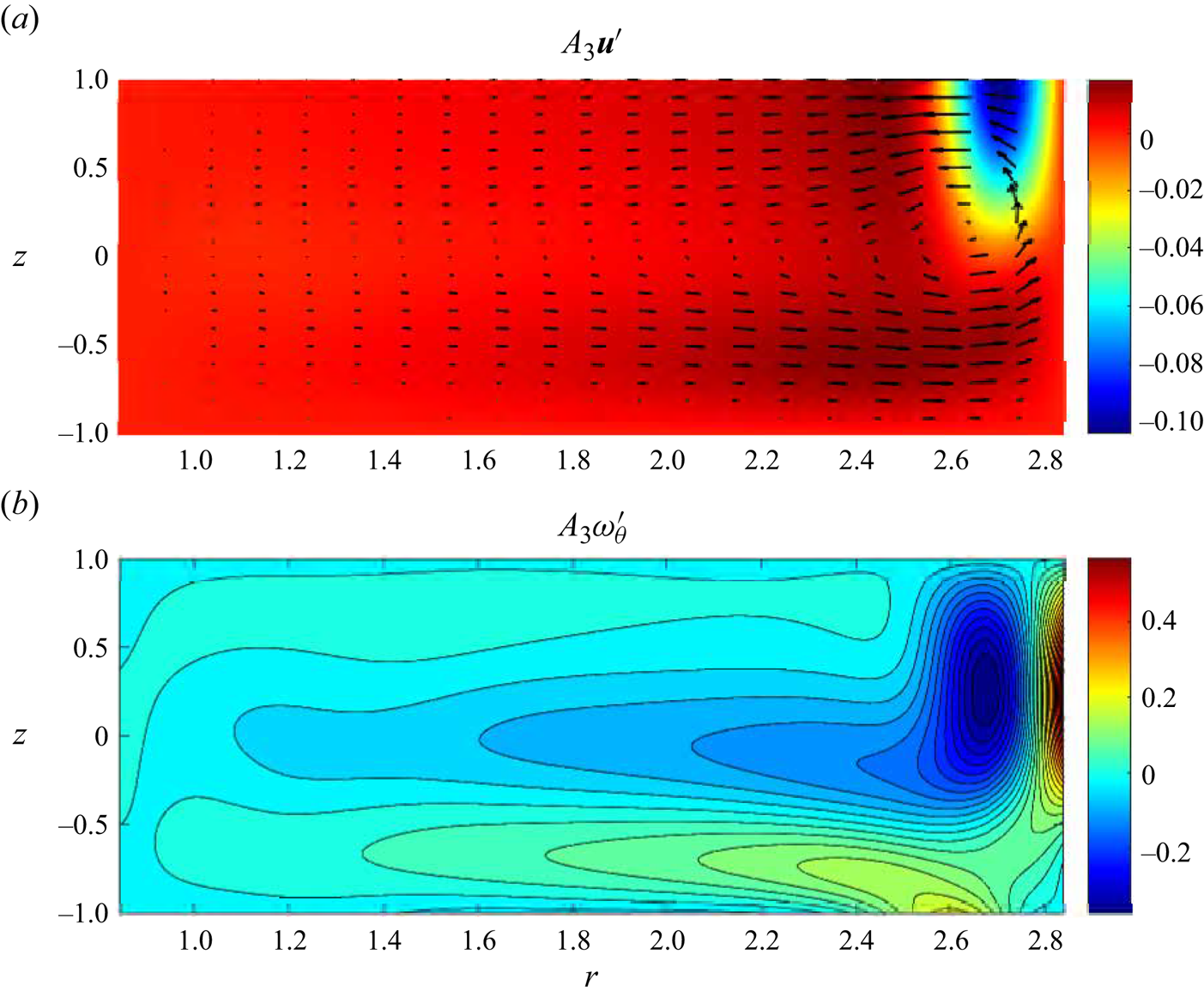
Figure 6. Meridional  $\theta$-independent linearised perturbation velocity (a) and azimuthal vorticity (b) fields for the same parameters as in figure 5.
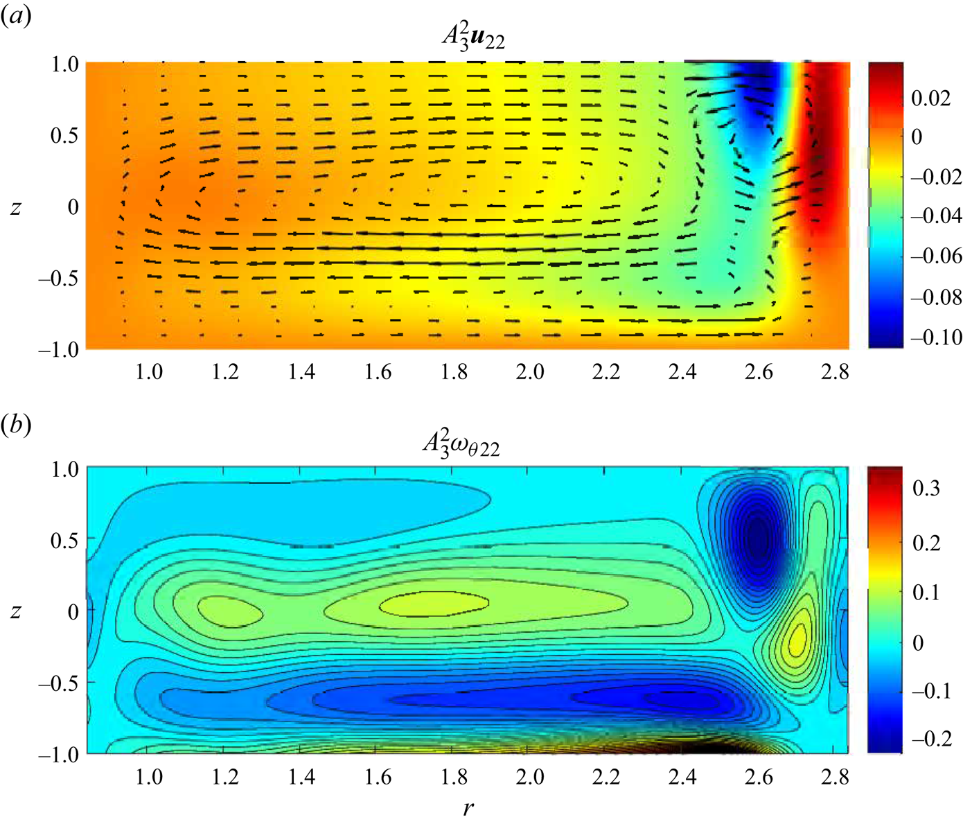
Figure 7. Second-order meridional  $\theta$-independent perturbation velocity (a) and azimuthal vorticity (b) fields for the same parameter values as in figure 5.
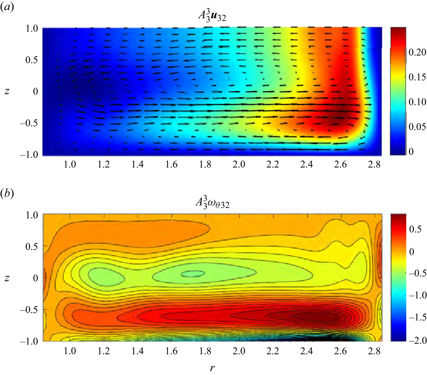
Figure 8. Third-order meridional  $\theta$-independent perturbation velocity (a) and azimuthal vorticity (b) fields for the same parameter values as in figure 5.
Figure 5 shows the converged Type 2 basic flow field. It corresponds to a toroidal flow, which, for lower Reynolds numbers, possess a secondary recirculation in the top outer corner of the meridional cross-section. However, for  $Re_0$ in the close vicinity of $Re_{**}$ the secondary circulation is completely suppressed so that visually the Type 2 solution depicted in figure 5 is indistinguishable from a typical Type 1 flow. However, such a basic flow is linearly weakly unstable (the growth rate $\sigma _0$ is slightly positive, see table 1) with respect to a perturbation that contains a prominent counter-rotating toroidal structure near the outer cylinder with the flow in the rest of the meridional plane almost not affected by it, see figure 6. It is also seen from figure 6(a) that the secondary circulation occurs along with the formation of an azimuthal jet near the corner between the outer cylinder and the free surface. It is directed against the main flow and, consequently, decelerates the overall azimuthal fluid motion there. Therefore, the secondary circulation occurs at the expense of energy taken from the local azimuthal flow.
The second-order perturbation field induced by the problem's nonlinearity enhances both this secondary toroidal structure and the primary meridional circulation of the basic flow and further retards azimuthal flow near the upper right corner, see figure 7. The secondary circulation near the right top corner is also enhanced by the third-order nonlinear perturbation shown in figure 8. However, the second- and third-order perturbations have opposite influences on the main flow structure in the meridional plane: while the second-order perturbations are characterised by clockwise main circulation, its third-order counterpart counteracts it with anti-clockwise motion in the bulk of fluid. The ultimate balance between these two influences leads to the existence of an equilibrium amplitude  $A_3$ defining the fixed point of (3.18), see the top circle in figure 3(a).
Figures 9 and 10 show the variation of the basic flow and the linearised perturbation fields with the parametric shift  $\delta$ away from the computational point $\varPi _0$, respectively. Even though the contribution of these variations to the overall balance is negligible given a very small parametric shift $\delta ={1500}/{1493.88}-1\approx 4.1\times 10^{-3}$ considered here, these figures demonstrate a noteworthy but somewhat counterintuitive tendency: the increase of Reynolds number, that is strengthening of electromagnetic flow forcing, leads to the decreasing intensity of both primary and secondary circulations (fluid circulation in figures 5 and 9 and in figures 6 and 10 occurs in opposite directions). From the energy point of view this cannot continue indefinitely and eventually as $Re$ increases the flow is forced to transition to a more energetic state, which provides a physical explanation to the detected fold catastrophe.
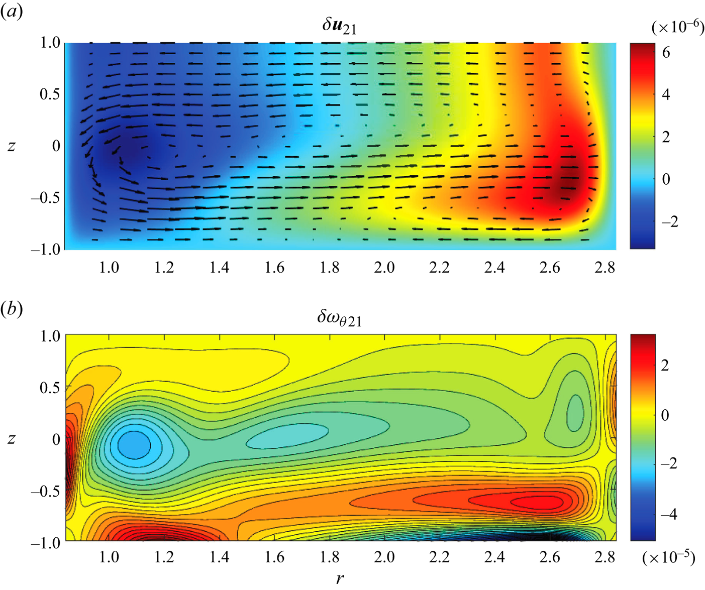
Figure 9. Meridional variation of  $\theta$-independent Type 2 basic flow velocity (a) and azimuthal vorticity(b) fields near the computational point $\varPi _0$ for the same parameters as in figure 5.
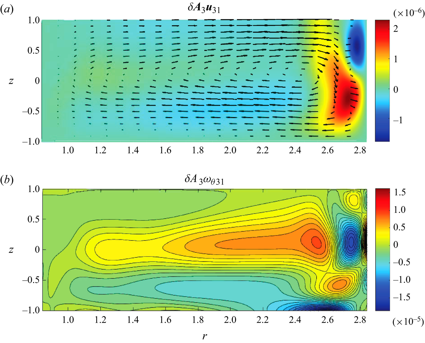
Figure 10. Third-order variation of meridional  $\theta$-independent perturbation velocity (a) and azimuthal vorticity (b) fields for the same parameters as in figure 5.
Figure 11 depicts the overall asymptotic solution (3.2) at  $Re=1500$. Despite the original basic flow shown in figure 5 having no visible secondary circulation, the reconstituted solution has it very strongly pronounced. Having constructed this asymptotic solution we now can use it as an initial guess for Newton iterations hoping to find the expected steady state that would differ from the previously reported Type 1 and 2 flows and exist for $Re>Re_{**}$. Reporting numerical implementation details of such an attempt are left for Part 2 of this study whereas here we state that indeed the derived asymptotic solution is found to be sufficiently close to the previously undetected steady state that we call the Type 3 flow so that Newton iterations do converge. The resulting field that represents the solution of nonlinear steady $\theta$-independent governing equations (2.2)–(2.6) obtained for $Re>Re_{**}$ is illustrated in figure 12. It is remarkable that while the approximate asymptotic solution shown in figure 11 differs from the full Type 3 solution illustrated in figure 12 quantitatively, it accurately captures all qualitative features of the full solution including the existence of the secondary circulation and of the submerged jet, where the magnitude of the azimuthal velocity component $v$ exceeds that at the free surface. This demonstrates once again the robustness of the asymptotic procedure developed here.
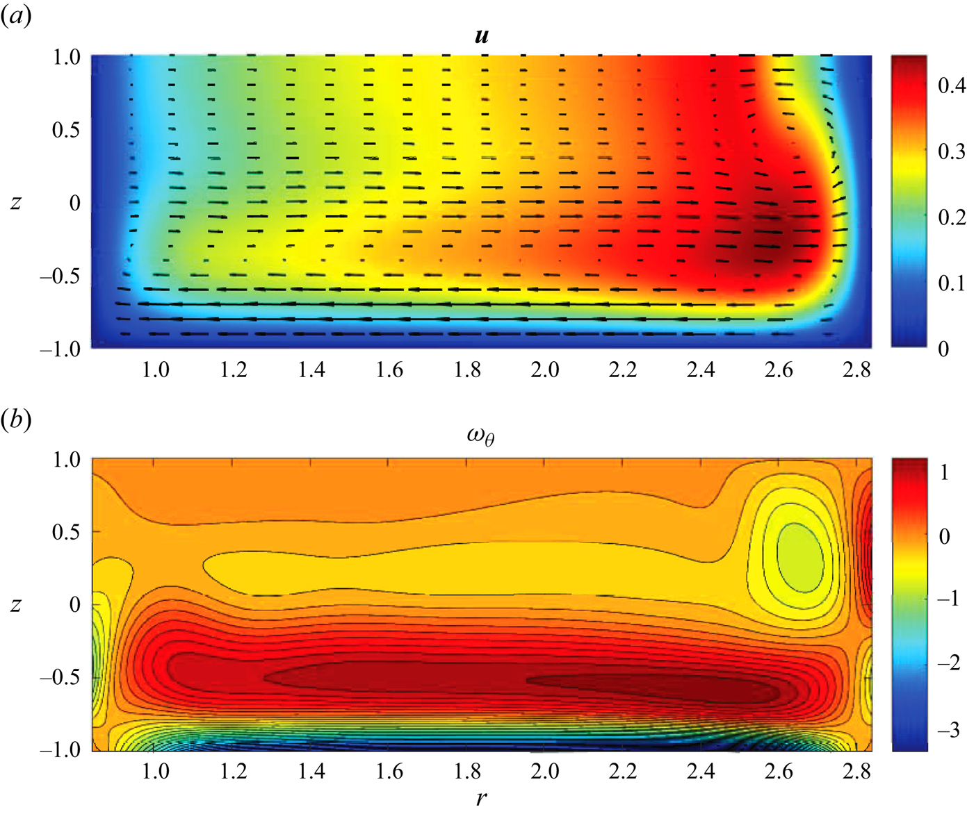
Figure 11. Approximation of the steady  $\theta$-independent component of the flow for $Re=1500>Re_{**}$: meridional velocity (a) and azimuthal vorticity (b) fields for the same values of $\epsilon$ and $ Ha $ as in figure 5.
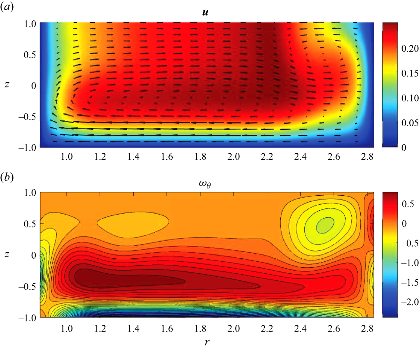
Figure 12. Full numerical steady  $\theta$-independent (Type 3) flow solution: meridional velocity (a) and azimuthal vorticity (b) fields for the same parameters as in figure 11.
Even though the analysis here says nothing about the stability of the steady  $\theta$-independent Type 3 flow that is different from both Type 1 and 2 basic flows investigated previously, our past studies (McCloughan & Suslov Reference McCloughan and Suslov2020a) demonstrated that the experimentally observable vortices arise on the free surface due to instabilities at the border between the two toroidal flow structures. Therefore, the new $\theta$-independent flow state obtained here has the necessary physical features to serve as a background for to the formation of such vortices in post-catastrophe regimes at $Re>Re_{**}$ as indeed will be confirmed in Part 2 of this study.
5. Cusp catastrophe
All numerical results presented so far have been obtained for a fixed value of  $\epsilon$. To complete the discussion we now turn to investigating what happens as the thickness of an electrolyte layer changes. A significant effort was invested into drawing a parametric existence map of the Type 1 and 2 steady $\theta$-independent basic flow solutions locating fold (saddle-node bifurcation) points by direct computations with parametric continuation in McCloughan & Suslov (Reference McCloughan and Suslov2020a). The weakly nonlinear consideration based on the third-order amplitude expansion developed in the present work offers a computationally much cheaper procedure for achieving the same goal and providing a much more insightful view of the arising flow structures.
In figure 13 we present the collection of fixed-point diagrams for (3.18) computed for various non-dimensional electrolyte layer depths  $\epsilon$. The individual S-shaped amplitude curves have two turning points. The one corresponding to a larger value of $Re$ approximates $Re_{**}$, where Type 1 and 2 basic flows annihilate each other in a local saddle-node bifurcation, see the blue solid line in figure 13(a,c). The red solid lines in the same panels connect the second fold points. Qualitatively, they correspond to $Re_{*}< Re_{**}$ at which the Type 2 solution ceases to exist as found in McCloughan & Suslov (Reference McCloughan and Suslov2020a). No conclusive evidence that at $Re_{*}$ the Type 2 solution is replaced with yet another $\theta$-independent solution different from both Type 1 and 2 flows was given in McCloughan & Suslov (Reference McCloughan and Suslov2020a) (a numerical steady-state solver used there failed to produce it starting from a random initial guess or using parametric continuation from the Type 2 solution). Yet, the S-shaped curves in figure 13 strongly suggest that such a flow topologically similar to the asymptotic solution shown in figure 11 should exist as indeed will be confirmed in Part 2 of this study.
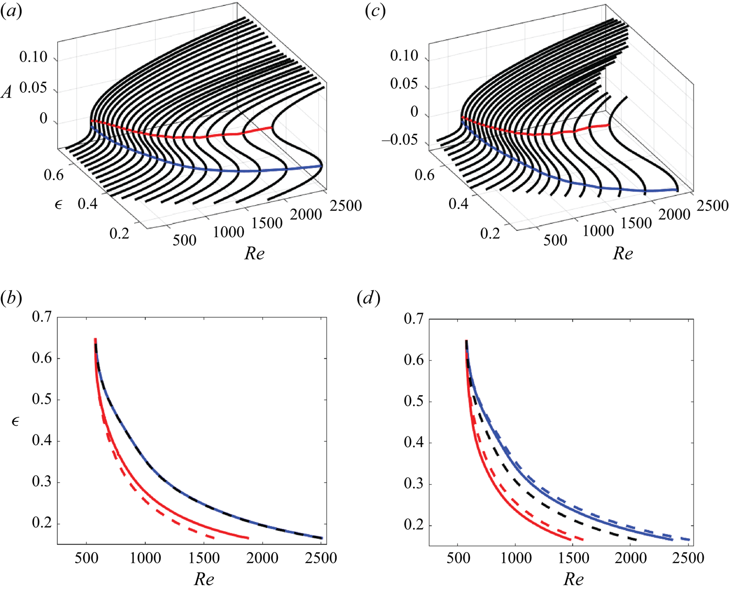
Figure 13. Cusp catastrophe diagrams computed for ( $a$,
$a$, $b$)
$b$)  $Re_0=Re_{*}+0.99(Re_{**}-Re_{*})$ and (c,d) $Re_0=(Re_{*}+Re_{**})/2$ in the $(Re,\epsilon )$ parametric space. The red and blue dashed lines in panels ( $b$) and ( $d$) correspond to the values $Re_{*}$ and $Re_{**}$, respectively, reported in McCloughan & Suslov (Reference McCloughan and Suslov2020a), the black dashed lines show the values $Re_0$ at which coefficients of (3.18) have been computed in each panel. The solid lines illustrate the positions of folds.
As the depth of the electrolyte layer increases, the difference between the two turning points of the S-shaped curves approaches zero at  $\epsilon \approx 0.649$ (which correspond to the depth of 19.6 mm in the experiments of Pérez-Barrera et al. Reference Pérez-Barrera, Pérez-Espinoza, Ortiz, Ramos and Cuevas2015, Reference Pérez-Barrera, Ortiz and Cuevas2016), where the fold disappears. Algebraically, this can be seen from (4.2) that in the limit $\sigma _0\to 0$ factorises to
 \begin{equation} A(2K_{31}K_{32}A^2+(K_{22}K_{31}+3K_{21}K_{32})A+2K_{21}K_{22})=0, \end{equation}
which has three solutions:  $A_1=0$ and
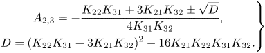 \begin{equation} \left.\begin{gathered} A_{2,3} ={-}\frac{K_{22}K_{31}+3K_{21}K_{32}\pm\sqrt{D}}{4K_{31}K_{32}}, \\ D=(K_{22}K_{31}+3K_{21}K_{32})^2-16K_{21}K_{22}K_{31}K_{32}. \end{gathered}\right\} \end{equation}
The behaviour of the discriminant  $D$ is shown in figure 14. When it becomes negative, the real amplitude solutions $A_{2,3}$ cease to exist. Therefore, $D=0$ corresponds to the two-parameter cusp catastrophe. Indeed, the projection of the lines connecting the two fold points in figure 13(a,c) onto the $(Re,\epsilon )$-plane (the solid blue and red lines) form a cusp shown in figure 13(b,d) with the fold existing between them.
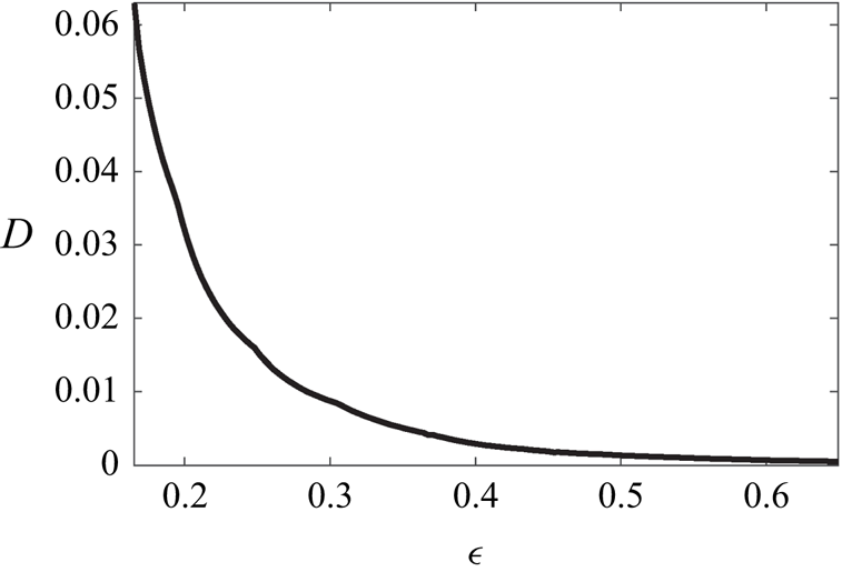
Figure 14. Variation of discriminant  $D$ given by (5.2) with non-dimensional layer thickness $\epsilon$.
The location of folds predicted by the analysis of (3.18) remains very close to the values of  $Re_{*}$ and $Re_{**}$ determined from very expensive direct numerical computations completed in McCloughan & Suslov (Reference McCloughan and Suslov2020a), compare the dashed and solid lines in figure 13(b,d). In figure 13(b) the coefficients of (3.18) were computed for $Re_0$ chosen close to $Re_{**}$ so that the dashed and solid blue lines are indistinguishable within the plot resolution. The difference between the parametric location of the second fold and $Re_{*}$ (the red lines) is noticeable, yet topologically the two curves are identical and lead to the same cusp location.
Of course, from a practical point of view one would wish to avoid expensive direct computations of the catastrophe points  $Re_{*}$ and $Re_{**}$ replacing them with a much less time-consuming analysis of (3.18). Thus, one generally cannot rely on choosing $\varPi _0$ at which its coefficients are to be computed to be close to $\varPi _*$ or $\varPi _{**}$ as they may not be known. To demonstrate the robustness of the developed analysis in figure 13(c,d) we present the cusp catastrophe diagrams computed using coefficients of (3.18) evaluated far away from both $Re_{*}$ and $Re_{**}$, namely, at a half of parametric distance between them, see the black dashed line in figure 13(d). Despite such a remote computational position, the predicted locations of $Re_{*}$ and $Re_{**}$ (the solid red and blue lines) remain close to the true values (the dashed lines) with the position of the cusp point determined accurately regardless of where the coefficients were computed.
Finally, we note that once the fold disappears in the cusp catastrophe the topologically different solutions obtained for the past-catastrophe parametric values are expected to morph into each other in a continuous way. This is indeed demonstrated in figure 15. It shows that as the strength of electric current (the magnitude of the Reynolds number) increases near the cusp catastrophe the single-torus flow field very quickly develops the secondary circulation. However, unlike in the fold catastrophe existing in thinner electrolyte layers, this transition occurs in a continuous way.
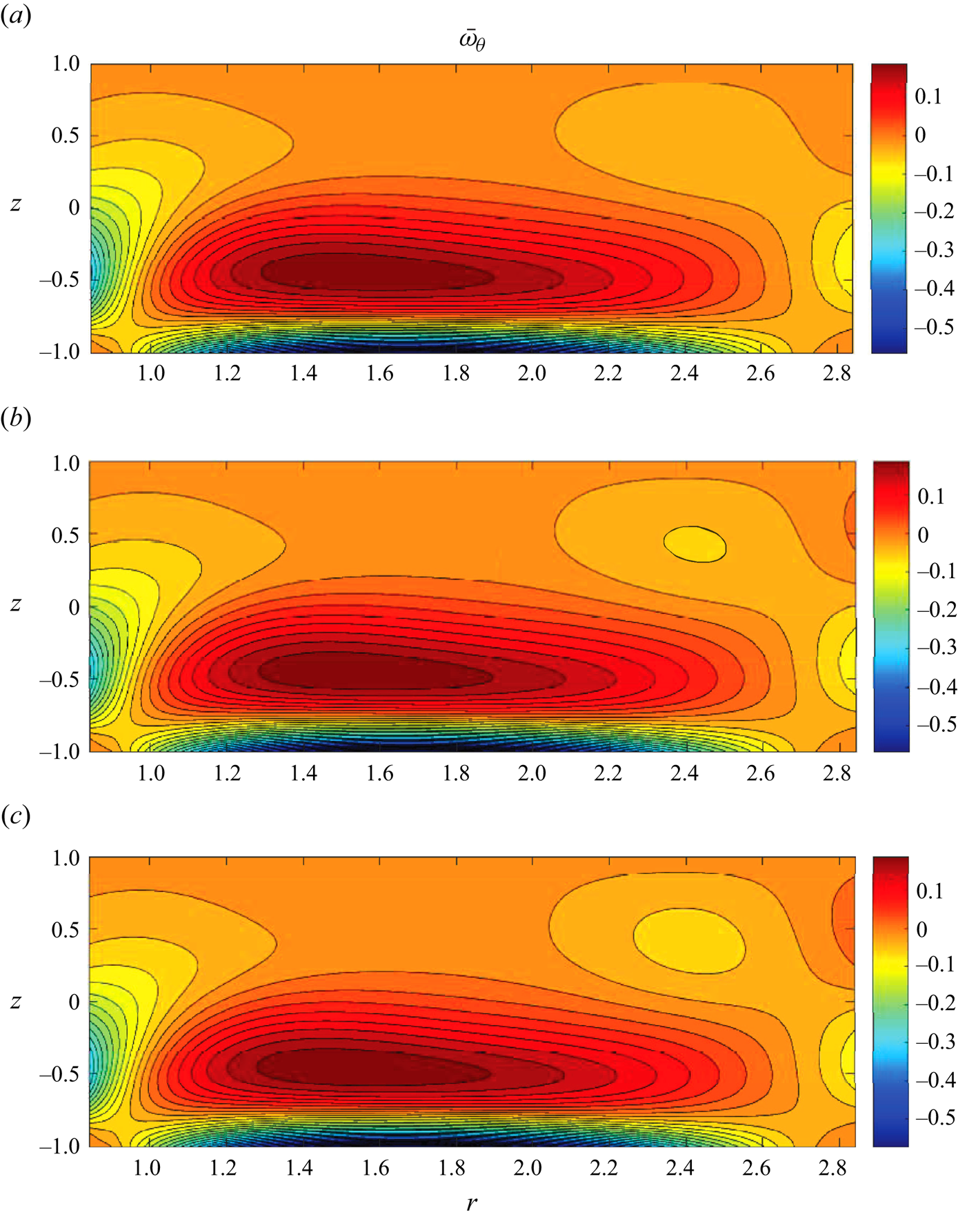
Figure 15. Rapid appearance of the secondary toroidal flow structure near the cusp catastrophe point: azimuthal vorticity fields computed for  $\epsilon =0.649$ ( $h=19.6$ mm), $ Ha =1.33\times 10^{-3}$ and (a) $Re=525$,(b) $Re=542$ and (c) $Re=559$ ( $I_0=0.030$, 0.031 and 0.032 A, respectively).
6. Is there a similarity with vortex breakdown or its variants?
Prior to concluding Part 1 of this study we touch upon a question that a reader familiar with other types of swirling flows in a cylindrical geometry may naturally ask: do the azimuthally invariant steady flows discussed in this paper bear any similarity with those described previously in the literature? Our past paper (Suslov et al. Reference Suslov, Pérez-Barrera and Cuevas2017b) has addressed it in length with the main conclusion being that despite a superficial similarity the electromagnetically bulk-driven flow considered here has no physically equivalent counterparts among mechanically induced flows. However, consideration in Suslov et al. (Reference Suslov, Pérez-Barrera and Cuevas2017b) was primarily given to boundary/shear layer-type flows as mentioned in the introduction in this paper. With the full topology of various steady azimuthally invariant flows bulk-driven by the Lorentz force in a shallow annular channel now being established, it is of interest to re-examine this conclusion in a specific context of vortex breakdown, the phenomenon that received much attention starting from the 1960s (Benjamin Reference Benjamin1962; Vogel Reference Vogel1968; Escudier Reference Escudier1984).
A classical vortex breakdown occurs in a closed cylinder filled with a fluid the swirling motion of which is driven by the rotation of one of the solid end walls (see, for example, Gelfgat, Bar-Yoseph & Solan (Reference Gelfgat, Bar-Yoseph and Solan1996) and Blackburn & Lopez (Reference Blackburn and Lopez2002) and references therein). The resulting Ekman layer is centrifugally driven towards the side wall next to it. The end-to-end symmetry is broken when the opposite wall of the container is either stationary or rotates with a different speed. The overall flow then consists of the fluid moving along the side wall from the quickly rotating end to the opposite and spiralling back near the axis of the vessel. Superficially, this may appear to be similar to the Type 1 flow in the context of the present study (with the obvious difference that the fluid has to move up along the inner solid cylinder in our case rather than to spiral down freely). As the rotation speed of the end wall increases the recirculation bubble near the axis of the cylinder forms and this is referred to as the vortex breakdown. Again, this may appear similar to the formation of a secondary circulation as in the Type 2 and 3 solutions reported here (with the difference that in our set-up the secondary circulation occurs near the outer stationary solid wall rather than at the axis). This is where the similarities stop. The physical reasons for that may be explained following the discussion in Shtern, del Mar Torregrosa & Herrada (Reference Shtern, del Mar Torregrosa and Herrada2012). These authors argue that the classical vortex breakdown is closely related to the so-called swirl decay, that is, to the fact that the influence of the end wall rotation driving the swirling motion of fluid decreases with the distance from it. This changes the balance between the centrifugal and viscous forces in the axial direction, which, in turn, creates non-monotonic variation of pressure along the axis, which ultimately causes the formation of recirculation bubbles and vortex breakdown along the axis. In other words, the reason why vortex breakdown becomes possible is that the source of the angular momentum is localised at the rotating end wall with the fluid dissipating it through friction at stationary solid walls and viscous shear in the bulk. The principle physical difference of the set-up considered in our study from that of the vortex breakdown is that the swirl decay mechanism is inactive here because the source of the angular momentum (Lorentz force) is distributed throughout the bulk of fluid. It is somewhat weaker near the free surface than at the bottom of the annulus due to the reduction of the magnetic field with the distance from the magnet on top of which the annulus rests, but in thin layers considered here such a reduction is inconsequential. Numerical experiments show that even if Lorentz force is assumed to be constant, this does not affect the existence of secondary circulations in the Type 2 and 3 solutions.
This fundamental physical distinction between electromagnetically bulk-driven flows and surface-induced vortex breakdown flows brings about further differences in how they depend on the two main governing parameters, the aspect ratio  $\varLambda =h/R_2$ and Reynolds number $Re$. The majority of the vortex breakdown results reported in literature have been obtained for sufficiently long cylinders with $\varLambda >1$ (for example, $\varLambda =2.5$ in Blackburn & Lopez (Reference Blackburn and Lopez2002), $\varLambda$ up to 4 in Gelfgat et al. (Reference Gelfgat, Bar-Yoseph and Solan1996) and Shtern et al. (Reference Shtern, del Mar Torregrosa and Herrada2012), $\varLambda =3.5, 4.6, 5.3$ in Lopez (Reference Lopez2012, and experimental works cited there)). Multiple azimuthally invariant solutions were reported in these studies for sufficiently large rotation speeds and it was found that they are not steady (Blackburn & Lopez Reference Blackburn and Lopez2002) and that their topological and temporal complexities increase with the aspect ratio. Our results indicate the opposite trend: all azimuthally invariant solutions remain steady and their topological complexity reduces as the thickness of the fluid layer increases (further discussion of this is given in Part 2).
The comparison of our present results obtained for thin annular layers with  $\varLambda <0.25$ with those for mechanically driven flows in similar short cylinders, perhaps, would be more meaningful. Unfortunately, to the best of the authors’ knowledge the data for such thin flows driven by a rotating end wall are rather limited, presumably because of the relative flow simplicity dictated by strong viscous dissipation that does not warrant detailed studies. For example, Gelfgat et al. (Reference Gelfgat, Bar-Yoseph and Solan1996) reports that only one-torus steady solution with no secondary circulation could be found for $\varLambda =0.5$. It is likely that this observation holds for even shorter cylinders (clearly, the swirl decay mechanism for vortex breakdown suggested in Shtern et al. (Reference Shtern, del Mar Torregrosa and Herrada2012) cannot work in thin layers). Therefore, we are led to conclude that physical trends we discovered for electromagnetically bulk-driven flows are significantly different to those existing in well-studied vortex breakdown flows with any analogy being only superficial. We also note that a recent study of the influence of the axial magnetic field on a flow of an electrically conducting fluid filling a cylinder with all or some conducting walls and a rotating bottom reported in Laouari et al. (Reference Laouari, Mahfoud, Bessaïh and Hadjadj2021) demonstrated that vortex breakdown is suppressed by the arising Lorentz force. However, this occurs at much larger values of Hartmann number $( Ha >15)$ than those relevant to a weak electrolyte used as a working fluid in the current work.
A variation of the vortex breakdown problem, where the opposite end walls of a cylinder co- or counter-rotate, has also received much attention in the literature. Such studies have been performed for relatively thin fluid layers and, thus, may potentially reveal features somewhat similar to those reported here. In particular, Lopez (Reference Lopez1998) used direct numerical simulations (DNS) to find two distinct stable azimuthally invariant steady states in a cylindrical flow between two counter-rotating discs. Subsequently, the author hypothesised that there should be a third, unstable and thus unaccessible by DNS, state sandwiched between the two stable flows in a parametric space. It was then qualitatively suggested that these three states could form a cusp/fold similar to that we computed and presented in figure 13 here with the Type 1 and 3 being stable and Type 2 unstable solutions (as shown in McCloughan & Suslov (Reference McCloughan and Suslov2020a) for the Type 1 and 2 flows and in Part 2 of this manuscript for the Type 3 state). Of course, the physical mechanisms responsible for the existence of multiple steady flow states, which are associated with topologically different boundary layer separation patterns, between two counter-rotating discs are completely different from those acting in a bulk-driven electrolyte layer, where boundary layers either do not exist (at the free surface) or remains safely attached (at the solid bottom).
Finally, we mention a set-up of a free-surface flow in a cylindrical tank with a rotating bottom (e.g. Spohn, Mory & Hoppinger Reference Spohn, Mory and Hoppinger1993, and references therein). In an idealised formulation the free surface is assumed to be flat, and this approximation has also been used in our computations, see Suslov et al. (Reference Suslov, Pérez-Barrera and Cuevas2017b) for justification. It might be tempting then to refer to such a similarity and argue the potential equivalence of the bottom-driven cylindrical flow set-up with bulk-driven flows investigated here. Following symmetry arguments Lopez et al. (Reference Lopez, Marques, Hirsa and Miraghaie2004) calculated azimuthally invariant steady flow states by doubling the height of the computational domain and treating the free surface as a symmetry plane of such an extended cylinder with co-rotating end walls. They found that steady flows computed for small values of aspect ratio ( $\varLambda =0.25$), which are of relevance here, contained a prominent solid-body-rotation core, the conclusion also confirmed by Yang et al. (Reference Yang, Delbende, Fraigneau and Witkowski2019) for computations performed accounting for a realistic free-surface deformation. No such structure has been found in flows discussed here. Therefore, reinforcing the arguments of Suslov et al. (Reference Suslov, Pérez-Barrera and Cuevas2017b) we are led to conclude that despite a superficial resemblance none of the well-studied wall-driven swirling flows share their features with flows caused by the action of the bulk Lorentz force.
7. Conclusions
Despite the geometric simplicity of an annular flow domain and of the electromagnetic forcing driving the primary circumferential fluid motion, the investigated flow reveals a surprisingly rich range of experimentally observable flow patterns that is shown to differ from other swirling flow set-ups such as vortex breakdown in a cylinder with a rotating end wall. The current study has focused primarily on the azimuthally invariant flow component. It continues the computational and analytic effort made in our previous study that discovered a saddle-node bifurcation in which two different steady flow patterns termed Type 1 and 2 in Suslov et al. (Reference Suslov, Pérez-Barrera and Cuevas2017b) and McCloughan & Suslov (Reference McCloughan and Suslov2020a) merge into one and then cease to exist as the Lorentz force driving the flow increases. The current study undertook a higher order (cubic) asymptotic analysis based on perturbation amplitude ( $A$) expansion. It enabled us to strengthen the hypothesis proposed in McCloughan & Suslov (Reference McCloughan and Suslov2020a) that another azimuthally invariant flow pattern exists for sufficiently large values of the radial current (and, thus, the driving Lorentz force parameterised by the Reynolds number $Re$). Such a pattern is different from Type 1 and 2 flows but has a secondary circulation that is qualitatively similar to that of Type 2 flow reported previously. In the amplitude-forcing $(A,Re)$ phase space, along with Type 1 and 2 flows such a pattern forms a classical fold catastrophe. The previously reported saddle-node bifurcation is found to be its local feature. Our subsequent consideration of flows arising in layers of different depths parameterised by the non-dimensional layer thickness $\epsilon$ has established that the discovered fold catastrophe is a part of a cusp catastrophe arising in the three-dimensional $(A,Re,\epsilon )$ space. Overall, azimuthally invariant flow patterns found for sufficiently strong forcing in past-fold- and past-cusp-catastrophe regimes are characterised by the presence of a secondary circulation flow structure near the corner formed by the outer cylindrical wall and the free surface.
We note that locating parametric positions of catastrophes mentioned above is a challenging task: the traced solutions cease to exist beyond the catastrophe point so that computationally one cannot ‘overshoot’ the bifurcation and then ‘come back and refine’. This breaks standard iterative search procedures that may be successful for, say, locating pitchfork bifurcations, where at least one solution exists on either side of the critical point. Thus, one has to rely on strictly one-sided-approach procedures that become unreliable in the vicinity of catastrophes or saddle-node bifurcations. To overcome such a difficulty we introduced a procedure for deriving amplitude equations describing canonical catastrophes that is capable of accurately estimating critical points without the need of approaching them asymptotically closely in a parametric space, which has the value of its own in a wider context than that of the considered physical problem.
It was argued in McCloughan & Suslov (Reference McCloughan and Suslov2020a) that the existence of the secondary circulation is a necessary condition for the appearance of experimentally observable anti-cyclonic vortices on the free surface. The current study shows that with the discovery of the Type 3 two-tori steady azimuthally invariant flow such a condition is satisfied for wide ranges of fluid layer depths and strengths of electromagnetic flow forcing, which can explain the robustness of free-surface vortices observed in experiments (Pérez-Barrera et al. Reference Pérez-Barrera, Pérez-Espinoza, Ortiz, Ramos and Cuevas2015, Reference Pérez-Barrera, Ortiz and Cuevas2016, Reference Pérez-Barrera, Ramírez-Zúñiga, Grespan, Cuevas and del Río2019). However, there are still a number of flow aspects that require further investigation that we will report in Part 2 of this study. In particular, it is of interest how such a steady flow establishes starting from a motionless state. To answer this question a time integration of the governing equation is required that we will undertake and report in Part 2. In Part 2 we also investigate the instability of the newly determined steady-state pattern, discuss how it leads to the formation of the experimentally observable free-surface anti-cyclonic vortex patterns in strong-forcing regimes and report their quantitative characteristics.
Declaration of interests
The authors report no conflict of interest.
Appendix A. Expressions appearing in weakly nonlinear expansions
The terms appearing in the right-hand sides of asymptotic equations appearing at the second and third order of perturbation amplitude in § 3 are
 \begin{align}
f_{21}^{(1)} =\frac{1}{Re_0}\left[\partial^2_r \bar{u}
+\frac{1}{r}\partial_r
\bar{u}-\frac{1}{r^2}\bar{u}+\frac{1}{\epsilon^2}\partial^2_z\bar{u}
+ Ha ^2\left(\bar{w} B_r-\frac{1}{\epsilon^2}\bar{u}
B_z\right)B_z\right],\end{align}
\begin{align}
f_{21}^{(1)} =\frac{1}{Re_0}\left[\partial^2_r \bar{u}
+\frac{1}{r}\partial_r
\bar{u}-\frac{1}{r^2}\bar{u}+\frac{1}{\epsilon^2}\partial^2_z\bar{u}
+ Ha ^2\left(\bar{w} B_r-\frac{1}{\epsilon^2}\bar{u}
B_z\right)B_z\right],\end{align}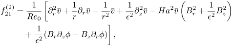 \begin{align}
f_{21}^{(2)}&=\frac{1}{Re_0}\left[\partial^2_r\bar{v}
+\frac{1}{r}\partial_r \bar{v}-\frac{1}{r^2} \bar{v}
+\frac{1}{\epsilon^2}\partial^2_z \bar{v} - Ha
^2\bar{v}\left(B_r^2+\frac{1}{\epsilon^2}
B_z^2\right)\right.\nonumber\\
&\quad + \left.\frac{1}{\epsilon^2}(B_r\partial_z
\phi-B_z\partial_r\phi)\right],
\end{align}
\begin{align}
f_{21}^{(2)}&=\frac{1}{Re_0}\left[\partial^2_r\bar{v}
+\frac{1}{r}\partial_r \bar{v}-\frac{1}{r^2} \bar{v}
+\frac{1}{\epsilon^2}\partial^2_z \bar{v} - Ha
^2\bar{v}\left(B_r^2+\frac{1}{\epsilon^2}
B_z^2\right)\right.\nonumber\\
&\quad + \left.\frac{1}{\epsilon^2}(B_r\partial_z
\phi-B_z\partial_r\phi)\right],
\end{align} \begin{gather}
f_{21}^{(3)}=\frac{1}{Re_0}\left[\partial^2_r
\bar{w}+\frac{1}{r}\partial_r \bar{w}
+\frac{1}{\epsilon^2}\partial^2_z \bar{w}+ Ha
^2\left(\frac{1}{\epsilon^2}\bar{u} B_z-\bar{w}
B_r\right)B_r\right],
\end{gather}
\begin{gather}
f_{21}^{(3)}=\frac{1}{Re_0}\left[\partial^2_r
\bar{w}+\frac{1}{r}\partial_r \bar{w}
+\frac{1}{\epsilon^2}\partial^2_z \bar{w}+ Ha
^2\left(\frac{1}{\epsilon^2}\bar{u} B_z-\bar{w}
B_r\right)B_r\right],
\end{gather}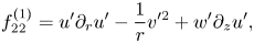 \begin{gather}
f_{22}^{(1)}
=u'\partial_ru'-\frac{1}{r}v'^2+w'\partial_zu',
\end{gather}
\begin{gather}
f_{22}^{(1)}
=u'\partial_ru'-\frac{1}{r}v'^2+w'\partial_zu',
\end{gather}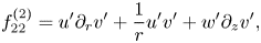 \begin{gather}
f_{22}^{(2)}
=u'\partial_rv'+\frac{1}{r}u'v'+w'\partial_zv',
\end{gather}
\begin{gather}
f_{22}^{(2)}
=u'\partial_rv'+\frac{1}{r}u'v'+w'\partial_zv',
\end{gather}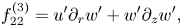 \begin{gather}
f_{22}^{(3)}=u'\partial_rw'+w'\partial_zw',
\end{gather}
\begin{gather}
f_{22}^{(3)}=u'\partial_rw'+w'\partial_zw',
\end{gather} \begin{align}
f_{31}^{(1)} &= u'\partial_r u_{21}+u_{21}\partial_r u'-\frac{2}{r} v'
v_{21} +w'\partial_zu_{21}+w_{21}\partial_ru'\nonumber\\
&\quad+\,\frac{1}{Re_0}\left[\left(\partial_r^2+\frac{1}{r}\partial_r-\frac{1}{r^2}
+\frac{1}{\epsilon^2}\partial_z^2\right)u' + Ha ^2\left( w'
B_r-\frac{1}{\epsilon^2}u'B_z\right)B_z\right]+2K_{21}u_{22},
\end{align}
\begin{align}
f_{31}^{(1)} &= u'\partial_r u_{21}+u_{21}\partial_r u'-\frac{2}{r} v'
v_{21} +w'\partial_zu_{21}+w_{21}\partial_ru'\nonumber\\
&\quad+\,\frac{1}{Re_0}\left[\left(\partial_r^2+\frac{1}{r}\partial_r-\frac{1}{r^2}
+\frac{1}{\epsilon^2}\partial_z^2\right)u' + Ha ^2\left( w'
B_r-\frac{1}{\epsilon^2}u'B_z\right)B_z\right]+2K_{21}u_{22},
\end{align}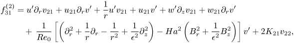 \begin{align}
f_{31}^{(2)} &=u'\partial_rv_{21}+u_{21}\partial_r
v'+\frac{1}{r}u'v_{21} +u_{21}v'+w'\partial_z
v_{21}+w_{21}\partial_rv'\nonumber\\ &\quad
+\,\frac{1}{Re_0}\left[\left(\partial_r^2+\frac{1}{r}\partial_r-\frac{1}{r^2}
+ \frac{1}{\epsilon^2}\partial_z^2\right) - Ha ^2\left(
B_r^2+\frac{1}{\epsilon^2}
B_z^2\right)\right]v'+2K_{21}v_{22},
\end{align}
\begin{align}
f_{31}^{(2)} &=u'\partial_rv_{21}+u_{21}\partial_r
v'+\frac{1}{r}u'v_{21} +u_{21}v'+w'\partial_z
v_{21}+w_{21}\partial_rv'\nonumber\\ &\quad
+\,\frac{1}{Re_0}\left[\left(\partial_r^2+\frac{1}{r}\partial_r-\frac{1}{r^2}
+ \frac{1}{\epsilon^2}\partial_z^2\right) - Ha ^2\left(
B_r^2+\frac{1}{\epsilon^2}
B_z^2\right)\right]v'+2K_{21}v_{22},
\end{align}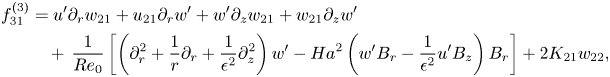 \begin{align}
f_{31}^{(3)} &=u'\partial_r w_{21}+u_{21}\partial_rw'+w'\partial_z
w_{21}+w_{21}\partial_zw'\nonumber\\ &\quad
+\,\frac{1}{Re_0}\left[\left(\partial_r^2+\frac{1}{r}\partial_r
+\frac{1}{\epsilon^2}\partial_z^2\right)w' - Ha ^2\left(
w'B_r-\frac{1}{\epsilon^2}u'B_z\right)B_r\right]+2K_{21}w_{22},
\end{align}
\begin{align}
f_{31}^{(3)} &=u'\partial_r w_{21}+u_{21}\partial_rw'+w'\partial_z
w_{21}+w_{21}\partial_zw'\nonumber\\ &\quad
+\,\frac{1}{Re_0}\left[\left(\partial_r^2+\frac{1}{r}\partial_r
+\frac{1}{\epsilon^2}\partial_z^2\right)w' - Ha ^2\left(
w'B_r-\frac{1}{\epsilon^2}u'B_z\right)B_r\right]+2K_{21}w_{22},
\end{align} \begin{gather}
f_{32}^{(1)} =u'\partial_r
u_{22}+u_{22}\partial_ru'-\frac{2}{r}v'v_{22}
+w'\partial_zu_{22}+w_{22}\partial_zu'+2K_{22}u_{22},
\end{gather}
\begin{gather}
f_{32}^{(1)} =u'\partial_r
u_{22}+u_{22}\partial_ru'-\frac{2}{r}v'v_{22}
+w'\partial_zu_{22}+w_{22}\partial_zu'+2K_{22}u_{22},
\end{gather} \begin{gather}
f_{32}^{(2)}
=u'\partial_rv_{22}+u_{22}\partial_rv'+\frac{1}{r}u'v_{22}
+\frac{1}{r} u_{22}v'+w'\partial_zv_{22}+w_{22}\partial_zv'
+2K_{22}v_{22},
\end{gather}
\begin{gather}
f_{32}^{(2)}
=u'\partial_rv_{22}+u_{22}\partial_rv'+\frac{1}{r}u'v_{22}
+\frac{1}{r} u_{22}v'+w'\partial_zv_{22}+w_{22}\partial_zv'
+2K_{22}v_{22},
\end{gather} \begin{gather}
f_{32}^{(3)} =u'\partial_rw_{22}+u_{22}\partial_rw'+w'\partial_zw_{22}
+w_{22}\partial_zw'+2K_{22}w_{22}.
\end{gather}
\begin{gather}
f_{32}^{(3)} =u'\partial_rw_{22}+u_{22}\partial_rw'+w'\partial_zw_{22}
+w_{22}\partial_zw'+2K_{22}w_{22}.
\end{gather}


 Open access