2.1. Constraints from spatial symmetries

In three dimensions, the rank-four viscosity tensor $\eta _{ijk\ell }$ has 81 possible elements. However, the form of the viscosity tensor is constrained by the symmetries of the fluid it describes. For example, the most general form of the viscosity tensor for an isotropic fluid is given by

(2.1)\begin{equation} \eta_{i j k \ell} = \zeta \delta_{ij} \delta_{k \ell} + \mu \big( \delta_{ik} \delta_{j \ell } + \delta_{i\ell } \delta_{jk} - \tfrac{2}{3} \delta_{ij} \delta_{k \ell } \big) + \eta_{\text{R}} (\delta_{ik} \delta_{j \ell} - \delta_{i \ell} \delta_{jk}), \end{equation}

which contains just three independent coefficients: the shear viscosity $\mu$, the bulk viscosity $\zeta$ and the rotational viscosity $\eta _{{R}}$ (de Groot Reference de Groot1962). These three coefficients are invariant under parity: the exact same coefficients describe the evolution of a fluid and the image of the fluid in a mirror. In an anisotropic fluid, however, this need not be the case.

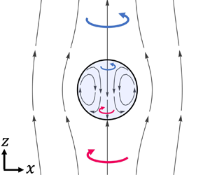
To systematically classify all the viscosity coefficients compatible with a given set of symmetries, we use the language of group theory. A general introduction to group theory in the context of fluid mechanics and applied mathematics is given in Cantwell (Reference Cantwell2002) and Hydon, Hydon & Crighton (Reference Hydon, Hydon and Crighton2000). Readers unfamiliar with this formalism can skip directly to (2.7), which generalizes the expression in (2.1). Figure 1 and table 2 provide a visual summary of the possible symmetries of the fluid illustrated by microscopic examples, along with the allowed entries in the viscosity tensor for each symmetry class. In general, the less symmetry the fluid has (moving down figure 1), the larger the number of independent viscosity coefficients. Our symmetry analysis can also be read as a guide on how to build parity-violating fluids from microscopic constituents. The symmetry of the fluid can be designed using the interplay between the symmetries of the microscopic constituents and the way these constituents are collectively arranged in the fluid (for instance, whether they are aligned); see figure 1(a–g) and accompanying caption for concrete examples.

Figure 1. Axial symmetry groups, examples of their microscopic realizations and their constraints on the viscosity tensor. (a–g) Examples of microscopic systems for each axial point group (with cylindrical symmetry about the $\boldsymbol {\hat {z}}$ axis) in (h). Each example is distinguished from the others by the presence of or absence of additional spatial symmetries. (a) A fluid of spherical particles is invariant under all rotations and reflections. (b) A fluid of randomly oriented helices (with fixed chirality) is invariant under all rotations, but no reflections. (c) A fluid of elongated (nematic) particles that align with each other is invariant under reflections across all planes parallel and perpendicular to the $\boldsymbol {\hat {z}}$ axis. (d) A fluid of chiral particles that align is invariant under ${\rm \pi} /2$ rotations about any axis perpendicular to the $\boldsymbol {\hat {z}}$ axis, but not any reflections. (e) A fluid of electric dipoles under an electric field is invariant under reflections across all planes parallel, but not perpendicular, to the $\boldsymbol {\hat {z}}$ axis. (f) A fluid of charged particles under a magnetic field (or a fluid of active particles rotating about a fixed axis) is invariant under reflections across all planes perpendicular, but not parallel, to the $\boldsymbol {\hat {z}}$ axis. (g) A fluid of chiral particles that rotate about a fixed axis has no additional symmetry beyond cylindrical. The group–subgroup relations between axial point groups are shown by arrows in (h). Groups drawn in identical colour place identical constraints on the viscosity tensor. The groups $K_h \equiv O(3)$ and $K\equiv SO(3)$ (in black) give rise to the viscosity tensor of an isotropic fluid in (2.1). The groups $D_{\infty h}$, $C_{\infty v}$ and $D_\infty$ (in blue) allow all the coefficients in black in (2.7) and table 2. Some of these coefficients are anisotropic, and all are invariant under reflections parallel and perpendicular to the $\boldsymbol {\hat {z}}$ axis (even though the microscopic components are not necessarily invariant under such reflections). The groups $C_{\infty h}$ and $C_\infty$ allow for additional coefficients that change sign under reflection across planes containing the $\boldsymbol {\hat {z}}$ axis. These coefficients are shown in red in (2.7) and table 2. For more details of the symmetry groups, see Shubnikov (Reference Shubnikov1988) and Hahn (Reference Hahn2005) (in particular table § 10.1.4.2, p. 799; and figure § 10.1.4.3, p. 803).

We begin by noting that under a rotation or reflection of space, the viscosity tensor transforms as

(2.2)\begin{equation} \eta_{i j k \ell} = {\mathsf{R}}_{i i'} {\mathsf{R}}_{j j'} {\mathsf{R}}_{k k'} {\mathsf{R}}_{\ell \ell'} \eta_{i' j' k' \ell'}, \end{equation}

where $\boldsymbol{\mathsf{R}}$ is an orthogonal matrix that implements the transformation. We say a fluid is parity-violating if its properties are not invariant under some improper rotation, i.e. a rotation combined with a reflection. In three dimensions, the most general viscosity tensor invariant under all proper rotations (i.e. under the group $SO(3)$, consisting of the transformations $\boldsymbol{\mathsf{R}} \in O(3)$ with $\det (\boldsymbol{\mathsf{R}}) = 1$) is automatically invariant under all improper rotations as well (i.e. under the whole group $O(3)$). This happens because any improper rotation can be written as a proper rotation times $-\mathbb {1} = \operatorname {diag}(-1,-1,-1)$: the four copies of $- \mathbb {1}$ always cancel out of (2.2).

Hence, we have to consider anisotropic fluids in order to see the effects of parity violation. Here, we focus on systems with cylindrical symmetry (i.e. those invariant under rotation about a fixed axis $\hat {\boldsymbol {z}}$). The set of all reflections and rotations that leave a fluid globally unchanged forms a group $G$. It turns out that there are just nine possible symmetry groups that respect cylindrical symmetry (Shubnikov Reference Shubnikov1988; Hahn Reference Hahn2005). These groups, known as the axial point groups, are shown in figure 1 and differ from each other by which combinations of horizontal and/or vertical reflections are present (see Appendix B, in particular figure 7). Just as invariance under $O(3)$ and $SO(3)$ placed identical constraints on the viscosity tensor, some of the anisotropic symmetry groups in figure 1 place identical constraints on the viscosity tensor. They break into two classes, drawn in blue and in red in figure 1. Fluids with the symmetry groups $D_{\infty {h}}$, $C_{\infty {v}}$ or $D_{\infty }$ (in blue) have an anisotropic viscosity tensor that is invariant under all reflections parallel and perpendicular to the $\hat {\boldsymbol {z}}$ axis. We call these fluids parity-preserving cylindrical, and examples include aligned nematic particles ($D_{\infty {h}}$), aligned helices ($C_{\infty v}$) and dipolar molecules in an electric field ($C_{\infty v}$) shown in figure 1(c–e). In contrast, fluids with the symmetry groups $C_{\infty h}$ or $C_{\infty }$ (in red) allow additional terms in their viscosity tensor. Examples of such fluids shown in figure 1(f,g) include spherical charged particles ($C_{\infty {h}}$) and chiral charged particles ($C_{\infty }$) in a magnetic field. The additional allowed viscosity coefficients acquire a minus sign when reflected across any plane containing the $\hat {\boldsymbol {z}}$ axis. We call these fluids parity-violating cylindrical.

It is useful to organize the components of the viscosity tensor by decomposing the stress $\sigma _{ij}$ and velocity gradient $\dot {e}_{k \ell } \equiv \partial _\ell v_k$ tensors on a basis of $3 \times 3$ matrices $\tau _{ij}^A$ ($A = 1 \dots 9$) corresponding to a decomposition into irreducible representations of the orthogonal group $O(3)$ (see Appendix B). In this notation, the viscosity tensor $\eta _{ijk\ell }$ is expressed as a $9 \times 9$ matrix (see Scheibner, Irvine & Vitelli (Reference Scheibner, Irvine and Vitelli2020a) and Scheibner et al. (Reference Scheibner, Souslov, Banerjee, Surowka, Irvine and Vitelli2020b), in which this notation is also used to describe elastic and viscoelastic media). The basis consists of

1. (i) a diagonal matrix $\tau _{i j}^1 = {\mathsf{C}}_{ij} = \sqrt {\frac {2}{3}}\delta _{ij}$ corresponding to pressure and dilation,

2. (ii) three anti-symmetric matrices $\tau _{i j}^{A+1} = {\mathsf{R}}_{ij}^A = \epsilon _{Aij}$ corresponding to torques and vorticity, and

3. (iii) five traceless symmetric matrices $\tau _{i j}^{A+5} = {\mathsf{S}}^A_{ij}$ corresponding to shear stresses and shear strain rates, whose expressions are

(2.3)\begin{equation} \left.\begin{gathered} \boldsymbol{\mathsf{S}}^1 =\begin{bmatrix} 1 & 0 & 0 \\ 0 & -1 & 0 \\ 0 & 0 & 0 \end{bmatrix},\quad \boldsymbol{\mathsf{S}}^2 = \begin{bmatrix} 0 & 1 & 0 \\ 1 & 0 & 0 \\ 0 & 0 & 0 \\ \end{bmatrix},\quad \boldsymbol{\mathsf{S}}^3 = \begin{bmatrix} \frac{-1}{\sqrt{3}} & 0 & 0 \\ 0 & \frac{-1}{\sqrt{3}} & 0 \\ 0 & 0 & \frac{2}{\sqrt{3}} \\ \end{bmatrix},\\ \boldsymbol{\mathsf{S}}^4 = \begin{bmatrix} 0 & 0 & 0 \\ 0 & 0 & 1 \\ 0 & 1 & 0 \\ \end{bmatrix},\quad \boldsymbol{\mathsf{S}}^5 = \begin{bmatrix} 0 & 0 & 1 \\ 0 & 0 & 0 \\ 1 & 0 & 0 \\ \end{bmatrix}. \end{gathered}\right\} \end{equation}

Note that $\tau _{ij}^A \tau _{ij}^B = 2 \delta ^{AB}$. Defining

(2.4a–c)\begin{equation} \sigma^A \equiv \sigma_{ij} \, \tau_{ij}^A, \quad \dot{e}^A \equiv \dot{e}_{i j} \, \tau_{ij}^A,\quad \eta^{AB} = \tfrac{1}{2} \tau_{ij}^A \, \eta_{ijk\ell} \, \tau_{k\ell}^B, \end{equation}

we may write

(2.5)\begin{equation} \sigma^A = \eta^{AB} \, \dot{e}^B. \end{equation}

We can transform back to Cartesian tensors via

(2.6a–c)\begin{equation} \sigma_{ij} = \tfrac{1}{2} \,\sigma^A \tau_{ij}^A, \quad \dot{e}_{ij} = \tfrac{1}{2} \, \dot{e}^A \tau_{ij}^A, \quad \eta_{ijk\ell} = \tfrac{1}{2} \, \tau_{ij}^A \, \eta^{A B} \, \tau_{k\ell}^B. \end{equation}

The most general form of $\eta ^{A B}$ satisfying cylindrical symmetry about the $\boldsymbol {\hat {z}}$ axis is

(2.7)

in which the parity-violating viscosities are written in red (these are only allowed in the groups drawn in red in figure 1). An explicit list of parity-violating viscosities is also given in the caption of table 2. Concretely, these entries of the viscosity tensor relate components of the strain rate and stress tensors with different parities under a reflection by a mirror plane containing the $\hat {z}$ axis (see table 1 for the parities of the basis tensors used in (

) under the reflection $P_y$). Finally, we have restricted our attention to fluids invariant under continuous rotations about the $\hat {\boldsymbol {z}}$ axis, because they arise when an originally isotropic fluid is submitted to a single external field. In general, the fluid can be even less symmetric, for example when the fluid is invariant under a discrete point group. This can happen when multiple external fields that are not parallel to each other are applied, or in electron fluids in crystals (Cook & Lucas Reference Cook and Lucas2019; Rao & Bradlyn Reference Rao and Bradlyn2020; Toshio, Takasan & Kawakami Reference Toshio, Takasan and Kawakami2020; Varnavides et al. Reference Varnavides, Jermyn, Anikeeva, Felser and Narang2020).

Table 1. Effect of the reflection $P_y$ on the components of the stress and strain rate used in (2.7). The components with a $1$ are invariant under $P_y$, while those with a $-1$ change sign. The action of $P_y$ on Cartesian coordinates is $\operatorname {diag}(1,-1,1)$.

Table 2. Classes of viscosity tensors and allowed viscosity coefficients. The coefficients refer to (2.7). Parity-violating viscosities (those only present in the last column) are highlighted in red. Explicitly, these are ${\eta _A^{e}}$, ${\eta _{Q,2}^e}$, ${\eta _{Q,3}^e}$, ${\eta _{R}^o}$, ${\eta _1^o}$, ${\eta _2^o}$, ${\eta _A^{o}}$, ${\eta _{Q,2}^o}$, ${\eta _{Q,3}^o}$. See Hahn (Reference Hahn2005) for more details of the symmetry groups.

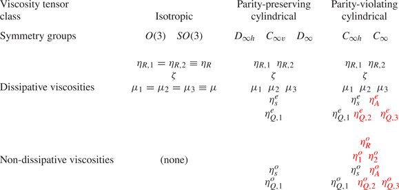
2.2. Dissipative and non-dissipative viscosities

In addition to the decomposition based on spatial symmetries discussed in § 2.1, the viscosity tensor can be decomposed into symmetric and anti-symmetric parts:

(2.8)\begin{equation} \eta_{ijk\ell} = \eta^{{e}}_{ijk\ell} + \eta^{{o}}_{ijk\ell}, \end{equation}

in which $e/o$ (standing for even/odd) label the symmetric and anti-symmetric parts of the tensor, satisfying $\eta ^{{o}}_{ijk\ell } = - \eta ^{{o}}_{k\ell ij}$ and $\eta ^{{e}}_{ijk\ell } = \eta ^{{e}}_{k\ell ij}$. The rate of mechanical energy lost by the fluid due to viscous dissipation is (see Appendix C.1)

(2.9)\begin{equation} \dot{w} = \sigma_{ij} \, \partial_j v_i = \eta_{i j k \ell} \, (\partial_j v_i) \, (\partial_\ell v_k) = \tfrac{1}{2} \, \eta^{A B} \dot{e}^A \dot{e}^B. \end{equation}

Hence, the anti-symmetric part $\eta ^{{o}}_{ijk\ell }$ is purely non-dissipative, because $\eta ^{{o}}_{ijk\ell } (\partial _j v_i) \, (\partial _\ell v_k) = 0$. In contrast, the symmetric part $\eta ^{\text {e}}_{ijk\ell }$ does indeed contribute to viscous dissipation. In a standard fluid, the viscous dissipation corresponds to a rate of entropy production $\dot s = (1/T) \, \sigma _{ij} \partial _j v_i$, where $T$ is temperature. The symmetry of the viscosity tensor has also been related to Onsager reciprocity relations in equilibrium fluids, in which one expects $\eta ^{{o}}_{ijk\ell } = 0$ when microscopic reversibility is satisfied (Onsager Reference Onsager1931; de Groot & Mazur Reference de Groot and Mazur1954; de Groot Reference de Groot1962).

The dissipative part $\eta ^{{e}}_{ijk\ell }$ of the viscosity tensor corresponds to the symmetric part of the matrix $\eta ^{A B}$ in (2.5), while the non-dissipative part $\eta ^{{o}}_{ijk\ell }$ corresponds to its anti-symmetric part. Hence, we have split all off-diagonal terms in (2.7) into odd and even parts (except when one of these is already ruled out by spatial symmetry). The non-dissipative viscosities all have an ‘o’ superscript. In table 2, we classify the viscosity coefficients in (2.7) based on whether they are dissipative or not, and on the symmetry groups in which they can occur.

4.1. Oseen tensor and Stokeslet

The (transient) Stokes equation for an incompressible fluid found in (1.3) can be written as

(4.1)\begin{equation} \rho \partial_t v_i ={-} \partial_i P + \partial_j [\eta_{i j k \ell} \partial_\ell v_k] + f_i \quad \text{with} \ \partial_i v_i = 0, \end{equation}

in which we have used the expression (1.2) of the viscous stress. In reciprocal space (see Appendix A for Fourier transform conventions):

(4.2)\begin{equation} -\text{i} \omega \rho v_i ={-} \text{i} q_i P - q_j q_\ell \eta_{i j k \ell} v_k + f_i \quad\text{with}\ \text{i} q_i v_i = 0. \end{equation}

These equations can be written as

(4.3)\begin{equation} \boldsymbol{\mathsf{M}}(\boldsymbol{q}, \omega) \boldsymbol{v} ={-} \text{i} P \boldsymbol{q} + \boldsymbol{f} \quad\text{with}\ \boldsymbol{q} \boldsymbol{\cdot} \boldsymbol{v} = 0, \end{equation}

in which we have defined the matrix

(4.4)\begin{equation} {\mathsf{M}}_{i k}(\boldsymbol{q}, \omega) = q_j q_\ell \eta_{i j k \ell} - \text{i} \omega \rho \, \delta_{i k}. \end{equation}

The matrix $\boldsymbol{\mathsf{M}}(\boldsymbol {q}, \omega )$ is always invertible at finite $\boldsymbol {q}$ provided that the dissipation rate $\dot {w}$ in (2.9) is strictly positive (see Appendix C.1). Under this hypothesis, we apply $M^{-1}(\boldsymbol {q}, \omega )$ to (4.3). We then take the scalar product with $\boldsymbol {q}$ to obtain the pressure $P$, and then replace $P$ with its expression to obtain the velocity, giving

(4.5a,b)\begin{equation} \text{i} P = \frac{\boldsymbol{q} \boldsymbol{\cdot} (\boldsymbol{\mathsf{M}}^{{-}1} \boldsymbol{f})}{{\boldsymbol{q} \boldsymbol{\cdot} (\boldsymbol{\mathsf{M}}^{{-}1} \boldsymbol{q})}}\quad\text{and}\quad \boldsymbol{v} ={-} \frac{{\boldsymbol{q} \boldsymbol{\cdot} (\boldsymbol{\mathsf{M}}^{{-}1} \boldsymbol{f})}}{{\boldsymbol{q} \boldsymbol{\cdot} (\boldsymbol{\mathsf{M}}^{{-}1} \boldsymbol{q})}} \, \boldsymbol{\mathsf{M}}^{{-}1} \boldsymbol{q} + \boldsymbol{\mathsf{M}}^{{-}1} \boldsymbol{f}. \end{equation}

The expression of the velocity in terms of the force is then

(4.6)\begin{equation} \boldsymbol{v} = \boldsymbol{\mathsf{G}}(\boldsymbol{q}, \omega) \boldsymbol{f}, \end{equation}

in which

(4.7)\begin{equation} {\mathsf{G}}_{ij} (\boldsymbol{q}, \omega) \equiv \left( [{\mathsf{M}}^{{-}1}]_{ij} - \frac{ [{\mathsf{M}}^{{-}1}]_{im}q_m q_n [{\mathsf{M}}^{{-}1}]_{nj} }{q_k [{\mathsf{M}}^{{-}1}]_{k\ell} q_\ell } \right)\end{equation}

is the Green function of the Stokes equation, which is usually called the (reciprocal space) Oseen tensor (Kim & Karrila Reference Kim and Karrila1991; Kuiken Reference Kuiken1996). Formally, it is defined so that $v_{i} = {\mathsf{G}}_{i j}$ is a solution of (4.1) with $\boldsymbol {f} = \delta (\boldsymbol {x}) \boldsymbol {e}_j$, where $\boldsymbol {e}_j$ is the unit vector in direction $j$. For an isotropic incompressible fluid, we recover the usual (reciprocal space) Oseen tensor

(4.8)\begin{equation} {\mathsf{G}}_{ij}^{{iso}}(\boldsymbol{q}, \omega=0) = \frac{1}{\mu q^2} \left(\delta_{ij} - \frac{q_i q_j}{q^2} \right). \end{equation}

When the symmetric part of $\eta _{ijk\ell }$ (corresponding to dissipation) vanishes, the second term of (4.7) diverges at $\omega = 0$ (but finite $\boldsymbol {q}$) because ${\mathsf{M}}^{-1}_{k \ell }$ is strictly anti-symmetric under exchange of $k$ and $\ell$, while the product $q_k q_\ell$ is symmetric (so the denominator $q_k [M^{-1}]_{k\ell } q_\ell$ vanishes). This corresponds to a divergence of the characteristic time scale associated with viscous relaxation: in this case, the Stokes approximation is not valid. In the following, we assume that viscous relaxation is fast enough, and focus on steady solutions that correspond to the steady Oseen tensor $\boldsymbol{\mathsf{G}}(\boldsymbol {q}) \equiv \boldsymbol{\mathsf{G}}(\boldsymbol {q}, \omega = 0)$.

The real-space Oseen tensor is then

(4.9)\begin{equation} {\mathsf{G}}_{i j}(\boldsymbol{x}) = \frac{1}{(2{\rm \pi})^3}\int {\text{e}}^{{\text{i}} \boldsymbol{q} \boldsymbol{\cdot} \boldsymbol{x}} \, {\mathsf{G}}_{i j}(\boldsymbol{q}) \, \text{d}^3 q \end{equation}

and the flow generated by a point force $\boldsymbol {f}(\boldsymbol {x}) = \boldsymbol {f} \delta (\boldsymbol {x})$ is the Stokeslet

(4.10)\begin{equation} \boldsymbol{v}(\boldsymbol{x}) = \boldsymbol{\mathsf{G}}(\boldsymbol{x}) \boldsymbol{f}. \end{equation}

When the anti-symmetric (non-dissipative) part of the viscosity tensor vanishes ($\eta _{ijk\ell }^o = 0$), the matrix $\boldsymbol{\mathsf{M}}$ defined by (4.4) is symmetric. Hence, ${\mathsf{M}}^{-1}$ and the Green function $\boldsymbol{\mathsf{G}}(\boldsymbol {q})$ are symmetric as well. The symmetry of the reciprocal-space Green function ${\mathsf{G}}_{i j}(\boldsymbol {q}) = {\mathsf{G}}_{j i}(\boldsymbol {q})$ is equivalent to ${\mathsf{G}}_{i j}(\boldsymbol {x}) = {\mathsf{G}}_{j i}(\boldsymbol {x})$ in physical space. This is the expression of Lorentz reciprocity (Masoud & Stone Reference Masoud and Stone2019, § 4.2, (4.7)), which can be interpreted as a symmetry in the exchange between the source (producing a force) and the receiver (measuring the velocity field). Conversely, Lorentz reciprocity is broken by the presence of non-dissipative (or, equivalently, odd) viscosities.

We can now analyse the effect of parity-violating viscosities on the Stokeslet. Unlike the situation in a two-dimensional, isotropic incompressible fluid (see Appendix D), in three dimensions the odd and parity-violating viscosities can modify the Stokeslet velocity field. To see this, we compute the real-space Oseen tensor or Stokeslet in different cases, using both numerical and analytical methods. The qualitative changes compared with usual isotropic fluids can be anticipated without any computation from symmetry arguments. When the driving force is along the axis of azimuthal symmetry, a fluid from the classes ‘isotropic’ and ‘parity-preserving cylindrical’ in table 2 cannot exhibit an azimuthal flow because a reflection symmetry constrains the azimuthal component of the velocity to be opposite to itself – this is indeed the case for the standard Stokeslet solution (Kim & Karrila Reference Kim and Karrila1991). In contrast, an azimuthal flow is allowed when parity-violating terms are introduced in the viscosity tensor (class ‘parity-violating cylindrical’ in table 2).

4.2. Stresslet, rotlet and multipolar responses

Since the Stokeslet is a response to a point perturbation, multipolar responses can be computed by taking derivatives of the Green function in (4.9) (see  Kim & Karrila Reference Kim and Karrila1991). For example, consider a force dipole defined by a point force $\boldsymbol {f}$ at $\frac 12 \delta \boldsymbol {r}$ and a point force $-\boldsymbol {f}$ at $-\frac 12 \delta \boldsymbol {r}$. The corresponding fluid velocity is given by

(4.11)\begin{equation} v_i( \boldsymbol{r}) = {\mathsf{G}}_{ik} \big(\boldsymbol{r} - \tfrac12 \delta \boldsymbol{r}\big) f_k - {\mathsf{G}}_{ik} \big(\boldsymbol{r} + \tfrac12\delta \boldsymbol{r}\big) f_k \approx{-}\partial_j {\mathsf{G}}_{ik} (\boldsymbol{r}) \delta r_j f_k \equiv {\mathsf{H}}_{ijk} (\boldsymbol{r}) \delta r_j f_k. \end{equation}

The tensor ${\mathsf{H}}_{ijk}$ is often decomposed into two contributions: the symmetric part ${\mathsf{S}}_{ijk} = \frac 12( {\mathsf{H}}_{ijk} + {\mathsf{H}}_{ikj} )$, which represents the response to point shears (also known as stresslet), and the anti-symmetric part $A_{i\ell } = \frac 12 \epsilon _{jk \ell } {\mathsf{H}}_{ijk}$, which represents the response to point torques $T_\ell$ (also known as rotlet). As discussed in § 3, such point torques can arise from a hydrostatic torque in the fluid. An explicit expression of the Oseen tensor ${\mathsf{G}}_{i k}$ is given by (H6) of Appendix H in a perturbative case, from which the stresslet and rotlet can be deduced using (4.11).

4.3. General numerical solution

To determine the physical-space Stokeslet or Oseen tensor $G(\boldsymbol {x})$, one must compute the inverse Fourier transform (4.9). This can be done numerically in the general case, in which analytical solutions are not easily accessible. To do so, we evaluate (4.7) on a discrete grid in reciprocal space (each component of $\boldsymbol {q}$ ranges from $-Q$ to $+Q$ with increments $\delta q$). This allows us to resolve length scales larger than a few ${\rm \pi} /Q$ but smaller than ${\rm \pi} /\delta q$. We then use the fast Fourier transform algorithm to compute the real-space Oseen tensor (or the real-space Stokeslet). To avoid numerical instabilities (Gibbs oscillations) due to the sharp cutoff in reciprocal space, we regularize the integrand in (4.9) with a Gaussian kernel $\exp ({- {\rm \pi}q^2/ 4 Q^2})$ (Cortez Reference Cortez2001; Gómez-González & del Álamo Reference Gómez-González and del Álamo2013). This procedure allows us to compute the Stokeslet for an arbitrary viscosity tensor. Our code for this computation is available at https://github.com/talikhain/StokesletFFT.

We consider an external force parallel to the $\hat {\boldsymbol {z}}$ axis and examine the perturbative effect of each coefficient separately. We set the normal shear viscosity to $\mu _1= \mu _2 = \mu _3 = 1$ and vary each of the other viscosity coefficients one by one, setting them to be $\eta _i = 0.01 \mu$. This flow is visualized for each viscosity in figure 8 of Appendix F, in which we also validate the numerical method using the exact solution discussed in the next section (see figure 10). We find that the viscosity coefficients that give rise to an azimuthal flow are

(4.12a–g) \begin{equation} \eta_R^o, \quad\eta^e_{Q,2}, \quad \eta^o_{Q,2}, \quad \eta^e_{Q,3}, \quad \eta^o_{Q,3}, \quad \eta_1^o, \quad \eta_2^o. \end{equation}

The list of viscosity coefficients that we found to generate $v_{\phi }$ are a subset of the parity-violating viscosities (in red in (2.7) and listed in the caption of table 2), as expected. In fact, the only parity-violating viscosities that do not give rise to azimuthal flow are $\eta ^e_A$ and $\eta ^o_A$. This is because we have assumed that the flow is incompressible. First, the term $(\eta _A^e - \eta _A^o) \boldsymbol {\nabla }\boldsymbol {\cdot } \boldsymbol {v}$ vanishes because $\boldsymbol {\nabla } \boldsymbol {\cdot } \boldsymbol {v} = 0$. Second, the term $(\eta _A^e + \eta _A^o) \omega _3$ contributes to the component $\sigma _C$ of the stress, and can therefore be absorbed in the pressure.

4.4. The Stokeslet of an odd viscous fluid: exact solution

We now consider a particular case in which the real-space Stokeslet can be computed analytically. First, we set $\mu \equiv \mu _1=\mu _2=\mu _3$ and consider only the odd shear viscosities $\eta _1^o$ and $\eta _2^o$ (all the other viscosities are assumed to vanish, except perhaps the bulk $\xi$ viscosity which drops out of the Stokes equation). In this case, the matrix $\boldsymbol{\mathsf{M}}(\omega = 0)$ defined by (4.4) takes the form

(4.13)\begin{equation} \boldsymbol{\mathsf{M}}(\omega = 0) =\begin{bmatrix} \mu q^2 & \eta_1^o(q_x^2 + q_y^2) - \eta_2^o q_z^2 & -\eta_2^o q_y q_z \\ - \eta_1^o(q_x^2 + q_y^2) + \eta_2^o q_z^2 & \mu q^2 & \eta_2^o q_x q_z \\ \eta_2^o q_y q_z & -\eta_2^o q_x q_z & \mu q^2 \end{bmatrix}. \end{equation}

Taking $\boldsymbol {f} = -\boldsymbol {\hat z} F_z \delta ^3(\boldsymbol {x})$, and defining $q_{\perp }^2 \equiv q_x^2 + q_y^2$, we find the full expressions for the velocity and pressure in Fourier space by using (4.5a,b):

(4.14) \begin{gather} \boldsymbol{\hat{v}(\boldsymbol{q})}= \frac{F_z}{N(\boldsymbol{q})} \begin{bmatrix} q_z(q_y(-(\eta_1^o + \eta_2^o)q_{{\perp}}^2 +\eta_2^o q_z^2) + \mu q_x (q_{{\perp}}^2 + q_z^2))\\ q_z(q_x((\eta_1^o+\eta_2^o)q_{{\perp}}^2 -\eta_2^o q_z^2) + \mu q_y (q_{{\perp}}^2 + q_z^2))\\ -\mu q_{{\perp}}^2(q_{{\perp}}^2 + q_z^2)\end{bmatrix}, \end{gather}

(4.15)\begin{gather}\hat{p}(\boldsymbol{q}) = {\text{i}} \frac{F_z}{N(\boldsymbol{q})} \, q_z[(\eta_1^o q_{{\perp}}^2 - \eta_2^o q_z^2)((\eta_1^o + \eta_2^o)q_{{\perp}}^2 - \eta_2^oq_z^2) + \mu^2(q_{{\perp}}^2 + q_z^2)^2]. \end{gather}

in which $N(\boldsymbol {q}) = \mu ^2(q_{\perp }^2 + q_z^2)^3+q_z^2((\eta _1^o + \eta _2^o)q_{\perp }^2 - \eta _2^o q_z^2)^2$. Second, we assume that $\eta _1^o = -2 \eta _2^o$, for which simplifications occur in (4.14)–(4.15). This particular case occurs in the limit of low magnetic field regime in experiments on polyatomic gases (see (13) in Hulsman et al. Reference Hulsman, Van Waasdijk, Burgmans, Knaap and Beenakker1970), and was also obtained in a theoretical Hamiltonian description of fluids of spinning molecules (Markovich & Lubensky Reference Markovich and Lubensky2021). In this limit, the viscosity matrix can be seen as a simple combination of isotropic contractions and rotations about the $\boldsymbol {\hat {z}}$ axis in the space of shears (see Appendix G).

In order to find the real-space solution, we compute the inverse Fourier transform in (4.9) (see Appendix G for the detailed calculation). Parameterizing the final flow field by $\gamma = \eta _2^o/ \mu$, we obtain the velocity field

(4.16)\begin{gather} v_r( {\Huge\unicode[Palace Script MT]{x0072}}, \theta) ={-}\frac{F_z}{4{\rm \pi} \eta_2^o}\frac{\cot{\theta}}{\gamma{\Huge\unicode[Palace Script MT]{x0072}}} \left(1 - \frac{1}{ \sqrt{1 + \gamma^2\sin^2\theta}}\right), \end{gather}

(4.17)\begin{gather}v_{\phi}({\Huge\unicode[Palace Script MT]{x0072}}, \theta) =\frac{F_z}{4{\rm \pi} \eta_2^o}\frac{\cot{\theta}}{{\Huge\unicode[Palace Script MT]{x0072}}} \left(1 -\frac{1}{ \sqrt{1+\gamma^2 \sin^2{\theta}}}\right), \end{gather}

(4.18)\begin{gather}v_z({\Huge\unicode[Palace Script MT]{x0072}}, \theta) =\frac{F_z }{4{\rm \pi} \eta_2^o } \frac{1}{ \gamma {\Huge\unicode[Palace Script MT]{x0072}}}\left(1 -\frac{\gamma^2 + 1}{ \sqrt{1+\gamma^2\sin^2 \theta}}\right), \end{gather}

as well as the pressure field

(4.19)\begin{equation} p({\Huge\unicode[Palace Script MT]{x0072}},\theta) =\frac{F_z}{4{\rm \pi}}\frac{\cos{\theta}}{{\Huge\unicode[Palace Script MT]{x0072}}^2}\left(1 - \frac{2(\gamma^2 + 1)}{(1 + \gamma^2 \sin^2{\theta})^{3/2}}\right) . \end{equation}

Here, ${\Huge\unicode[Palace Script MT]{x0072}}$ is the radius in spherical coordinates (see schematic in figure 2(a) and Appendix A). Streamlines of the velocity field are visualized for a range of $\gamma$ in figure 2 and supplementary movie 1 available at https://doi.org/10.1017/jfm.2021.1079. In the absence of odd viscosity, the Stokeslet flow only has two components, $v_r$ and $v_z$ (Appendix G), visualized in the vertical $x$–$z$ plane in figure 2(a) and in three dimensions in figure 2(b). Notably, as the blue and red arrows in figure 2(a) indicate, the flow develops an azimuthal component for $\gamma \neq 0$ (figure 2c–d), consistent with the fact that $\eta _1^o$ and $\eta _2^o$ are parity-violating (see table 2 and (2.7)).

Figure 2. A Stokeslet in an odd viscous fluid. (a) The streamlines of a standard Stokeslet flow are shown in black. The blue and red arrows indicate the appearance of an azimuthal flow once odd viscosity is introduced. A schematic of the system and the coordinate convention is shown in the inset. An external force, $\boldsymbol {F}$, is applied at the origin in the $-\hat {\boldsymbol {z}}$ direction. (b–d) A three-dimensional rendition of the Stokeslet streamlines initialized around a circle (i.e. many copies of the bold streamline in b), for a range of viscosity ratios, $\gamma = \eta ^o/\mu$. As the odd viscosity increases, the velocity field develops an azimuthal component that changes sign across the $z = 0$ plane, where the source is located. In the limit of only odd viscosity (d), the familiar radial component of the flow vanishes.

As $\gamma$ is increased, the magnitude of the azimuthal component grows, while the radial component diminishes. When $\gamma \gg 1$, the $\hat {\boldsymbol {r}}$ component of the velocity field goes to zero, while $v_{\phi }$ and $v_z$ approach $({\Huge\unicode[Palace Script MT]{x0072}} \sin {\theta })^{-1}$. (For the approximation of a steady Stokes flow to remain valid, the dissipative shear viscosity $\mu$ must remain finite in order to ensure that the relaxation time of the fluid is also finite, so the limit $\gamma = \infty$ is never actually reached.) At smaller $\gamma$, the central line splits into lobes of high azimuthal velocity that migrate away from the vertical, as illustrated in Appendix G.

4.5. Stokeslet: perturbative solution

In this section, we consider more generally the effect of the odd shear viscosities and of the rotational viscosities on the Stokeslet by treating the problem perturbatively (with respect to the small parameters characterizing the magnitude of these viscosities). We find that the first-order correction $\boldsymbol {v}_{\text {Stokes},1}$ to the standard Stokeslet (given in (G1) of Appendix G) due to the parity-violating coefficients $\eta _1^o, \eta _2^o$ and $\eta _R^o$ is of the form

(4.20)\begin{equation} \boldsymbol{v}_{\text{Stokes},1} = v_{\phi,1}\hat{\boldsymbol{\phi}} = \left[ v_{\phi, 1}^{(\eta_1^{o})} + v_{\phi, 1}^{(\eta_2^{o})} + v_{\phi, 1}^{(\eta_R^o)} \right] \hat{\boldsymbol{\phi}}. \end{equation}

Let us now discuss the explicit form of each of these terms, starting with the odd shear viscosities.

Starting back from (4.14)–(4.15) (in which $\eta _1^o$ and $\eta _2^o$ are independent), we perform a perturbative expansion in the quantities $\epsilon _{1(2)} \equiv \eta _{1(2)}^o/\mu \ll 1$. Computing the inverse Fourier transform to obtain the flow fields in real space as in § 4.4 (see Appendix H for the detailed calculation), we find that both $\eta _1^o$ and $\eta _2^o$ contribute to leading order by introducing terms contained entirely in the $\hat {\boldsymbol {\phi }}$ component of the velocity field. The contributions of the two viscosities are

(4.21)\begin{gather} v_{\phi, 1}^{(\eta_1^{o})}({\Huge\unicode[Palace Script MT]{x0072}},\theta)={-}\epsilon_1 \frac{F_z} {128 {\rm \pi}\mu}\frac{(5 + 3\cos{2\theta})\sin{2\theta}}{{\Huge\unicode[Palace Script MT]{x0072}}}+\mathscr{O}(\epsilon_1^2), \end{gather}

(4.22)\begin{gather}v_{\phi, 1}^{(\eta_2^{o})}({\Huge\unicode[Palace Script MT]{x0072}}, \theta)={-}\epsilon_2 \frac{F_z} {64 {\rm \pi}\mu } \frac{(1 + 3\cos{2\theta})\sin{2\theta}}{{\Huge\unicode[Palace Script MT]{x0072}}}+\mathscr{O}(\epsilon_2^2), \end{gather}

while the pressure is not modified at first order. The azimuthal component is visualized in the vertical $r$–$z$ plane in figure 3. In the absence of odd viscosity (figure 3a), $v_{\phi }=0$. The non-dimensionalized $v_{\phi }$ profiles for $\eta _1^o$ and $\eta _2^o$ given by (4.21)–(4.22) are shown in figure 3(b–c). While both velocity fields decay as $1/{\Huge\unicode[Palace Script MT]{x0072}}$, they differ appreciably in their angular dependence: $\eta ^o_2$ includes an additional sign change.

Figure 3. The non-dimensionalized azimuthal component of the Stokeslet flow for small shear and rotational odd viscosity coefficients. (a) In the absence of odd viscosity, the azimuthal component of the velocity field is zero. (b–d) The first-order correction of the Stokeslet due to $\eta _1^o, \eta _2^o$ and $\eta _R^o$, respectively, taking $\eta ^o/\mu = 0.1$. The origin is removed due to the singularity of the flow at $r = z = 0$. The azimuthal flow is odd with respect to $z$, and forms lobe-like regions of concentrated rotation. Blue indicates flow into the page, red corresponds to flow out of the page. Overall, the fluid flows out of the page in the upper lobe (in red) and into the page in the lower lobe (in blue). In (c), two small additional lobes have opposite velocities compared with the larger ones.

We now consider rotational viscosities, which couple vorticity and torques. These viscosities break both minor symmetries of the viscosity tensor ($\eta _{ijk\ell } \neq \eta _{jik\ell } \neq \eta _{ji\ell k}$), because the vorticity and torques are the anti-symmetric parts of the strain rate and stress tensors, and are shown in the block outlined in green in (2.7), reproduced below:

(4.23)\begin{equation} \begin{bmatrix} \sigma^1_R\\ \sigma^2_R\\ \sigma^3_R\end{bmatrix} = \begin{bmatrix} \eta_{R,1} & \eta_R^o & 0 \\ -\eta_R^o & \eta_{R,1} & 0 \\ 0 & 0 & \eta_{R,2} \end{bmatrix} \begin{bmatrix} \omega_1\\ \omega_2\\ \omega_3 \end{bmatrix} . \end{equation}

These rotational viscosities are often ignored in standard fluids because their contribution to the stress relaxes to zero over short times (de Groot Reference de Groot1962), but occur in the hydrodynamics of liquid crystals (Miesowicz Reference Miesowicz1946; Ericksen Reference Ericksen1961; Leslie Reference Leslie1968; Parodi Reference Parodi1970) as well as in the hydrodynamics of electrons in materials with anisotropic Fermi surfaces (Cook & Lucas Reference Cook and Lucas2019).

We consider perturbations in the quantities $\epsilon _{R,1} = \eta _{R,1}/\mu, \epsilon _{R,2} = \eta _{R,2}/\mu$ and $\epsilon _R^o = \eta _R^o/\mu$. The matrix $\boldsymbol{\mathsf{M}}$ is given by

(4.24)\begin{equation} \boldsymbol{\mathsf{M}} = \mu \begin{bmatrix} q^2 - \epsilon_{R,1} q_z^2 - \epsilon_{R,2}q_y^2 & \epsilon_{R,2} q_x q_y -\epsilon_R^o q_z^2 & \epsilon_{R,1} q_x q_z + \epsilon_R^o q_y q_z \\ \epsilon_{R,2} q_x q_y + \epsilon_R^o q_z^2 & q^2 -\epsilon_{R,1} q_z^2 - \epsilon_{R,2}q_x^2 & -\epsilon_R^o q_x q_z + \epsilon_{R,1} q_y q_z \\ \epsilon_{R,1} q_x q_z - \epsilon_R^o q_y q_z & \epsilon_R^o q_x q_z + \epsilon_{R,1} q_y q_z & q^2 - \epsilon_{R,1} q^2 \end{bmatrix}. \end{equation}

Applying (4.5a,b), we calculate the velocity and pressure in Fourier space:

(4.25)\begin{gather} \boldsymbol{v}(\boldsymbol{q}) = \frac{F_z}{\mu \, N_2(\boldsymbol{q})} \begin{bmatrix} - q_x q_z (q_{{\perp}}^2 + q_z^2) -\epsilon_R^o q_y q_z (q_{{\perp}}^2 + q_z^2) + \epsilon_R q_x q_z^3\\ - q_y q_z (q_{{\perp}}^2 + q_z^2) + \epsilon_R^o q_x q_z (q_{{\perp}}^2 + q_z^2) + \epsilon_R q_y q_z^3\\ q_{{\perp}}^2(q_{{\perp}}^2 + q_z^2) - \epsilon_R q_{{\perp}}^2 q_z^2 \end{bmatrix}, \end{gather}

(4.26)\begin{gather}p(\boldsymbol{q}) = \frac{-\text{i} Fz}{N_2(\boldsymbol{q})} \,[q_z (q_{{\perp}}^2 + q_z^2)^2 -\epsilon_R q_z (q_{{\perp}}^2 + q_z^2)(q_{{\perp}}^2 + 2q_z^2)+ (\epsilon_R^2 + (\epsilon_R^o)^2) q_z^3(q_{{\perp}}^2 + q_z^2)], \end{gather}

in which

(4.27)\begin{equation} N_2(\boldsymbol{q}) = {(q_{{\perp}}^2 + q_z^2)^3+ \epsilon_R(q_{{\perp}}^2 + q_z^2)^2({-}q_{{\perp}}^2 - 2q_z^2) + (\epsilon_R^2 + (\epsilon_R^o)^2)q_z^2 (q_{{\perp}}^2 + q_z^2)^2}. \end{equation}

Note that the coefficient $\epsilon _{R,2}$ does not affect the flow (see Appendix H for further details). For the remaining coefficients, we expand the above expressions up to first order in $\epsilon _{R,1}$ and $\epsilon _R^o$, and compute their inverse Fourier transform to find the real-space fields.

Of the three rotational viscosities, only $\eta _R^o$ violates parity (see table 2 and (2.7)) and as a consequence, gives rise to an azimuthal flow:

(4.28)\begin{equation} v_{\phi, 1}^{(\eta_R^o)}({\Huge\unicode[Palace Script MT]{x0072}},\theta)=\epsilon_R^o\frac{F_z}{16 {\rm \pi}\mu}\frac{\sin(2 \theta )}{ {\Huge\unicode[Palace Script MT]{x0072}}}+\mathscr{O}({(\epsilon_R^o)^2}) . \end{equation}

The $v_\phi$ profile due to $\eta _R^o$ is shown in figure 3(d). While the parity-violating shear and rotational viscosities generate quantitatively different azimuthal flows, their qualitative effect is the same. The pressure is again not modified to first order.

5.1. Odd viscous flow past a sphere

Two-dimensional flows past obstacles in the presence of a non-dissipative (odd) viscosity have previously been studied experimentally in Soni et al. (Reference Soni, Bililign, Magkiriadou, Sacanna, Bartolo, Shelley and Irvine2019) and theoretically in Kogan (Reference Kogan2016). Lapa & Hughes (Reference Lapa and Hughes2014) also analysed the consequences on swimmers at low Reynolds numbers. In these two-dimensional cases, only the pressure field is modified by the additional viscous terms, while the velocity field remains unchanged. Nevertheless, Kogan (Reference Kogan2016) reported that a lift force appears in the Oseen approximation (including inertia) of the flow past an infinite cylinder due to the non-dissipative viscosity. In this section, we consider three-dimensional flows. Even in the Stokes limit (without inertia), we find that parity-violating viscosities have a qualitative effect on the flow past a sphere: the Stokes drag is not modified at this order, but an azimuthal velocity develops despite the symmetry of the obstacle.

Let us begin by considering the viscous flow past a finite-radius sphere (Kim & Karrila Reference Kim and Karrila1991). We assume a uniform velocity field $\boldsymbol {v} =U \hat {\boldsymbol {z}}$ at ${\Huge\unicode[Palace Script MT]{x0072}} \to \infty$ and a no-slip boundary condition with $\boldsymbol {v}=0$ on the surface of the sphere ${\Huge\unicode[Palace Script MT]{x0072}} =a$. The streamlines of this flow in a standard fluid are shown in black in figure 4(a) on the $r$–$z$ plane. Here, we assume that the sphere cannot (or does not) rotate. In § 5.3, we discuss the case in which the sphere is allowed to rotate.

Figure 4. Odd viscous flow past (a–e) a sphere and (f–j) a bubble. (a) The streamlines of a standard flow past a sphere are shown in black. The blue and red arrows indicate the appearance of an azimuthal flow once odd viscosity is introduced. (b–e) The non-dimensionalized azimuthal velocity component of the flow visualized on the $r$–$z$ plane. If the odd viscosity is absent (b), the azimuthal component is zero. Perturbative additions of $\eta _1^o, \eta _2^o$ and $\eta _R^o$ (taking $\eta ^o/\mu = 0.1$) significantly affect the flow past a sphere by introducing a non-zero $v_{\phi }$ that is odd in $z$ (c–e). (f) The streamlines of a standard flow outside and inside a spherical bubble are shown in black. The blue and red arrows indicate the appearance of an azimuthal flow once odd viscosity is introduced. (g–j) The non-dimensionalized azimuthal velocity component of the flow visualized on the $r$–$z$ plane. Unlike the case of the sphere, the velocity field extends into the bubble, with a continuous velocity across the bubble surface. If the odd viscosity is absent (g), the azimuthal component is zero. Perturbative additions of $\eta _1^o$, $\eta _2^o$ and $\eta _R^o$ (taking $\eta ^o/\mu = 0.1$) significantly affect the flow by introducing a non-zero $v_{\phi }$ both inside and outside the bubble (h–j).

We once again look for a perturbative solution to (4.1) with $f_i = 0$ in the small parameters $\epsilon _1$, $\epsilon _2$ and $\epsilon _R^o$. To leading order in the parity-violating viscosities, the pressure field about the sphere is given simply by the pressure term due to the Stokeslet, as in a standard isotropic fluid. Since the Stokeslet pressure does not have a first-order correction (§ 4.5), (4.1) reduces to the vector Poisson equation for the first-order velocity field:

(5.1)\begin{equation} \Delta \boldsymbol{v_1} ={-} \varDelta_{\alpha} \boldsymbol{v_0}, \end{equation}

in which $\varDelta _{\alpha }$ is the second-order differential operator associated with the viscosity $\alpha$ (here, $\alpha = \eta _1^{o}, \eta _2^{o}, \eta _{R}^{o}$; see Appendix E for explicit form) and $\boldsymbol {v_0}$ is the flow past a sphere in a standard fluid (given by (I4)). The resulting vector Poisson equation for the perturbed flow is formally equivalent to the electrostatics problem of finding the electric potential due to a conducting spherical cavity enclosing a point charge. We use the corresponding Dirichlet Green function by expanding the solution in spherical harmonics (Jackson Reference Jackson1999). The details of this calculation are provided in Appendix I. Solving for the flow $\boldsymbol {v_1}$ to leading order in $\epsilon _1$, $\epsilon _2$ and $\epsilon _R^o$, we can express the resulting velocity field in terms of the Stokeslet solution, $\boldsymbol {v_{{Stokes}, 1}}$ in (4.21), (4.22) and (4.28), from § 4.5, as

(5.2)\begin{equation} v_{\phi, 1} ({\Huge\unicode[Palace Script MT]{x0072}}, \theta) =\left(\frac{6{\rm \pi} a U \mu}{F_z} \boldsymbol{v_{\text{Stokes}, 1}} + \frac{{\rm \pi} a^3 U \mu}{F_z}\Delta \boldsymbol{v_{\text{Stokes}, 1}} + \frac{{\rm \pi} a^5 U \mu}{20 F_z}\varDelta^2 \boldsymbol{v_{\text{Stokes}, 1}} \right)\boldsymbol{\cdot} \hat{\boldsymbol{\phi}} \end{equation}

with no modifications to $v_r$ and $v_z$ at leading order.

In standard isotropic fluids, a superposition of the Stokeslet ($v \propto 1/{\Huge\unicode[Palace Script MT]{x0072}}$) and its second derivative (a source dipole $v \propto 1/{\Huge\unicode[Palace Script MT]{x0072}} ^3$) is sufficient to satisfy the boundary conditions. In the presence of odd viscosity, we find that higher-order gradients are necessary, as can be seen from (5.2). Even so, by equating the far field of the flow and the Stokeslet solution, we find $F_z = 6{\rm \pi} a U\mu$. Hence, the Stokes drag experienced by the sphere remains unchanged to first order in $\eta _R^{o}$, $\eta _1^{o}$ and $\eta _2^{o}$ compared with a standard fluid.

Rewriting (5.2) more explicitly, we have

(5.3)\begin{equation} v_{\phi, 1} ({\Huge\unicode[Palace Script MT]{x0072}}, \theta) =\frac{3U}{64}\left[ g^1(\theta) \frac{a}{{\Huge\unicode[Palace Script MT]{x0072}}} + g^3(\theta) \left(\frac{a}{{\Huge\unicode[Palace Script MT]{x0072}}} \right)^3 + g^5(\theta) \left(\frac{a}{{\Huge\unicode[Palace Script MT]{x0072}}} \right)^5 \right] \sin{2\theta}, \end{equation}

where

(5.4)\begin{gather} g^1(\theta)=8\epsilon_R^o - ( 5 + 3\cos{2\theta} ) \epsilon_1 - (2 + 6\cos{2\theta}) \epsilon_2 +\mathscr{O}({\epsilon^2}) , \end{gather}

(5.5)\begin{gather}g^3(\theta)={-}8\epsilon_R^o + (6 +10\cos{2\theta}) \epsilon_1 + (4 +20\cos{2\theta}) \epsilon_2+\mathscr{O}({\epsilon^2}) , \end{gather}

(5.6)\begin{gather}g^5(\theta)={-}( 1 + 7\cos{2\theta} ) \epsilon_1 - (2 + 14\cos{2\theta}) \epsilon_2 +\mathscr{O}({\epsilon^2}). \end{gather}

These velocity fields are shown in figure 4(c–e) on the $r$–$z$ plane. As in the Stokeslet case, each odd viscosity coefficient results in an azimuthal flow, but the quantitative features of the velocity field vary depending on the exact viscosity chosen.

5.2. Odd viscous flow past a bubble

Closely related to the flow past a solid sphere is the flow past a spherical bubble without surface tension, in which the bubble itself is filled with a fluid (Hadamard Reference Hadamard1911; Rybczynski Reference Rybczynski1911; Lamb Reference Lamb1924; Batchelor Reference Batchelor1967). Here we assume that the inner and outer fluid have the same viscosities. As with the sphere, we solve for a steady velocity field configuration satisfying $\boldsymbol {v} = U \hat {\boldsymbol {z}}$ as ${\Huge\unicode[Palace Script MT]{x0072}} \to \infty$, but now we require that the velocity field be continuous throughout all space (even across the nominal boundary of the bubble). In a standard fluid, the flow outside the bubble resembles that of the flow past a sphere, while the flow inside is described by Hill's spherical vortex (Hill Reference Hill1894), with the boundary condition imposing continuous velocity at the surface. The streamlines of this velocity field are visualized in black in figure 4(f). Following the set-up above, let us consider the effect of the odd viscosities $\eta _1^o, \eta _2^o, \eta _R^o$ in the perturbative limit.

Like in the case of the sphere, the first-order correction to the pressure vanishes, and the flow outside the bubble reduces to (5.1). To solve this equation, we again employ Green function methods. Unlike the sphere problem, however, the boundary condition no longer requires no-slip velocity on the bubble surface, so we do not need to use the Dirichlet Green function. The details of this calculation are provided in Appendix J. Solving for the flow to leading order in $\epsilon _1$, $\epsilon _2$ and $\epsilon _R^o$, we can write it in terms of the Stokeslet solution, $\boldsymbol {v_{\text {Stokes}, 1}}$:

(5.7)\begin{equation} v_{\phi, 1}^{{out}} ({\Huge\unicode[Palace Script MT]{x0072}}, \theta) =\left(\frac{5{\rm \pi} a U \mu}{F_z} \boldsymbol{v_{\text{Stokes}, 1}} + \frac{{\rm \pi} a^3 U \mu}{2 F_z}\Delta \boldsymbol{v_{\text{Stokes}, 1}} + \frac{{\rm \pi} a^5 U \mu}{56 F_z}\varDelta^2 \boldsymbol{v_{\text{Stokes}, 1}} \right)\boldsymbol{\cdot} \hat{\boldsymbol{\phi}}, \end{equation}

with no modifications to $v_r$ and $v_z$ at leading order. As in the case of the sphere, the higher-order $1/{\Huge\unicode[Palace Script MT]{x0072}} ^5$ term is necessary to satisfy (5.1) and the boundary condition. By equating the far-field flow and the Stokeslet solution, we find $F_z = 5{\rm \pi} aU \mu$, which corresponds to the Stokesian drag on a bubble in a standard fluid; that is, the drag force is again unaffected at first order in odd viscosity. Note that the general form of the drag on a spherical bubble in a standard fluid is given by $F_z = (4{\rm \pi} a U \mu _{{out}} )(({\mu _{{out}} + ({3}/{2})\mu _{{in}}})/({\mu _{{out}} + \mu _{{in}}}))$, where $\mu _{{out}}$ and $\mu _{{in}}$ are the even shear viscosities outside and inside the bubble, respectively. In the case we are considering, $\mu _{{in}} = \mu _{{out}}$, so $F_z$ reduces to the expression above (Batchelor Reference Batchelor1967).

Rewriting (5.7) more explicitly, we have

(5.8)\begin{equation} v_{\phi, 1}^{{out}} ({\Huge\unicode[Palace Script MT]{x0072}}, \theta) =\frac{U}{896}\left[ g^1_{{out}}(\theta) \frac{a}{{\Huge\unicode[Palace Script MT]{x0072}}} + g^3_{{out}}(\theta) \left(\frac{a}{{\Huge\unicode[Palace Script MT]{x0072}}} \right)^3 + g^5_{{out}}(\theta) \left(\frac{a}{{\Huge\unicode[Palace Script MT]{x0072}}} \right)^5 \right] \sin{2\theta}, \end{equation}

where

(5.9)\begin{gather} g^1_{{out}}(\theta)= 280 \epsilon_R^o - (175 + 210 \cos{2\theta}) \epsilon_1 - (70 + 105\cos{2\theta}) \epsilon_2 +\mathscr{O}({\epsilon^2}), \end{gather}

(5.10)\begin{gather}g^3_{{out}}(\theta)={-}168 \epsilon_R^o + ( 126 + 210 \cos{2\theta}) \epsilon_1 + (84 + 420\cos{2\theta}) \epsilon_2+\mathscr{O}({\epsilon^2}), \end{gather}

(5.11)\begin{gather}g^5_{{out}}(\theta)={-}(15 + 105 \cos{2\theta}) \epsilon_1 - (30 + 210\cos{2\theta}) \epsilon_2 +\mathscr{O}({\epsilon^2}). \end{gather}

Next, we consider the flow inside the bubble. In this case, $\varDelta _{\alpha } \boldsymbol {v}_{\boldsymbol {0}}^{{in}} = 0$, so (4.1) reduces to the vector Laplace equation:

(5.12)\begin{equation} \Delta \boldsymbol{v}_{\boldsymbol{1}}^{{in}} = 0, \end{equation}

with the boundary condition $\boldsymbol {v}_{\boldsymbol {1}}^{{out}}(a, \theta ) = \boldsymbol {v}_{\boldsymbol {1}}^{{in}}(a, \theta )$. The solution to this Dirichlet problem involves the Dirichlet Green function used in the sphere computation (Jackson Reference Jackson1999) (see details in Appendix J). Solving for $\boldsymbol {v}_{\boldsymbol {1}}^{{in}}$, we find

(5.13)\begin{equation} v_{\phi, 1}^{{in}} ({\Huge\unicode[Palace Script MT]{x0072}}, \theta) = \frac{U}{56}\left[ g^1_{{in}}(\theta) \left(\frac{{\Huge\unicode[Palace Script MT]{x0072}}}{a}\right)^2 \right] \sin{2\theta}, \end{equation}

where

(5.14)\begin{equation} g^1_{{in}}(\theta)= 7\epsilon_R^o - 4\epsilon_1 - \epsilon_2 +\mathscr{O}({\epsilon^2}), \end{equation}

again with no modifications to $v_r$ and $v_z$ at leading order. We plot the velocity fields outside and inside the bubble in figure 4(h–j).

5.3. Effect of hydrostatic torque

As we have mentioned in § 3, parity-violating fluids, such as fluids made of spinning particles, can exhibit a hydrostatic torque $\sigma ^{h}_{ij} = -\epsilon _{ijz} \tau _z$ and a hydrostatic shear stress density in their hydrostatic stress. Let us illustrate the effect of the hydrostatic torque on a finite sphere. We assume a no-slip boundary condition at the surface of the sphere. In contrast to the situation of § 5.1, where the velocity at the surface of the sphere was assumed to vanish, here this velocity is determined by the balance between the torques due to the viscous stress and to the hydrostatic stress. Note that other boundary conditions could be appropriate, depending on the microscopic interactions between the constituents of the fluid and the boundary.

In the absence of odd viscosity, the hydrostatic torque leads to a total torque $T_z = \frac 83 {\rm \pi}a^3 \tau _z$ on the sphere (see (3.2)). Hence, the sphere rotates at a steady angular velocity $\varOmega = {T_z}/{8 {\rm \pi}a^3 \mu } = {\tau _z}/{3 \mu }$ (see Hobbie & Roth Reference Hobbie and Roth2007) and introduces an additional azimuthal component

(5.15)\begin{equation} v_\phi ({\Huge\unicode[Palace Script MT]{x0072}}, \theta) = \frac{\varOmega a^3 \sin \theta}{{\Huge\unicode[Palace Script MT]{x0072}}^2} \end{equation}

to the flow. This expression is valid for all ${\Huge\unicode[Palace Script MT]{x0072}}$ (in both near and far fields), as it satisfies the boundary condition. This azimuthal flow is even in $z$, unlike the flow due to the parity-violating viscosities, which is odd in $z$.

When odd viscosity is present, we can still compute the far-field flow using the perturbative Oseen tensor (computed in (H6) of Appendix H). The far-field flow is given by $v_i = A_{i z} T_z$ using the rotlet $A_{i \ell }$ (see § 4.2), and we find that

(5.16)\begin{equation} \boldsymbol{v} = \frac{T_z}{8{\rm \pi}\mu} \frac{\sin{\theta}}{{\Huge\unicode[Palace Script MT]{x0072}}^2}\boldsymbol{\hat{\phi}} + \epsilon \frac{T_z}{16{\rm \pi}\mu}\frac{1 + 3\cos{2\theta}}{{\Huge\unicode[Palace Script MT]{x0072}}^2} \hat{\boldsymbol{{\Huge\unicode[Palace Script MT]{x0072}}}}, \end{equation}

in which $\epsilon \equiv \eta ^o/\mu \ll 1$ and $\eta _2^o = - \eta _1^o /2 \equiv \eta ^o$. Again, we find an azimuthal flow even in $z$ as a consequence of the hydrostatic torque. In addition, we see that the presence of odd viscosity combined with a hydrostatic torque generates flow in the radial direction that is absent in the zeroth-order case.

6.1. Few particles: mechanisms

We now examine the role of parity-violating viscosities and of the corresponding azimuthal flows in the problem of sedimentation, in which particles driven by an external field (e.g. gravity) interact hydrodynamically at low Reynolds number. We assume the particles to be small identical spheres without inertia, which sediment under gravity and are advected by the flow due to the other particles.

In a standard isotropic fluid, an isolated sedimenting particle experiences a Stokesian drag and thus sinks at a velocity $U = F_z/(6{\rm \pi} \mu a)$. In a co-moving reference frame, the velocity field generated by a single sedimenting sphere $\beta$ is simply given by the Stokes flow past a sphere (I4). In the dilute limit, we can neglect the near-field terms that fall off faster than $1/{\Huge\unicode[Palace Script MT]{x0072}}$ (Happel Reference Happel1983). In particular, we neglect the higher-order $1/{\Huge\unicode[Palace Script MT]{x0072}} ^2$ velocity field contribution associated with particle rotation (see § 5.3), which may occur in a fluid with hydrostatic torques. As a result, the velocity field generated by each particle simply reduces to the Stokeslet (G1). If all the sedimenting particles experience the same force $\boldsymbol {f} = -\hat {\boldsymbol {z}}F_z$, the equation of motion in the co-moving frame for particle $\alpha$ becomes (Hocking Reference Hocking1964; Guazzelli et al. Reference Guazzelli, Morris and Pic2009)

(6.1)\begin{equation} \frac{{\text{d}}\kern0.7pt\boldsymbol{x}^{\alpha}}{{\text{d}}t} = \sum_{\alpha \neq \beta} G(\boldsymbol{x}^{\alpha} - \boldsymbol{x}^{\beta})\boldsymbol{f} , \end{equation}

where $G(\boldsymbol {x})$ is the Green function of the Stokes equation (Oseen tensor) from (4.9), $\alpha$ and $\beta$ are particle indices and $\boldsymbol {x}^\alpha$ is the position of particle $\alpha$ in the co-moving reference frame.

In a parity-violating fluid, we replace the standard Stokeslet field on the right-hand side of (6.1) with the odd viscous Stokeslet from (4.16)–(4.18). For simplicity, here we will consider $\eta _2^o = - \eta _1^o /2 \equiv \eta ^o$ and $\mu _1 = \mu _2 = \mu _3 \equiv \mu$ (all other viscosities in (2.7) are set to zero). Since each of the sedimenting particles experiences an identical vertical force, we can move into their co-moving reference frame. We then numerically integrate (6.1) over time with a standard fourth-order Runge–Kutta algorithm to obtain the trajectories of the particles.

Figure 5(a,b) shows the trajectories of three particles in the $x$–$z$ plane with $\eta ^o=0$ and $\eta ^o >0$. While the sedimentation of as few as three Stokeslets in a standard isotropic fluid is already chaotic (Hocking Reference Hocking1964; Jánosi et al. Reference Jánosi, Tél, Wolf and Gallas1997), the parity-violating flow introduces simple and well-defined modifications to the trajectories. For example, the trajectories of two particles interacting through the standard Stokeslet are confined to the vertical plane (figure 5c) containing initial positions. In the presence of odd viscosity, the particle trajectories are deflected out of this plane due to the azimuthal flow present in the odd Stokeslet (figure 5d). Similarly, the dynamics of a three-particle system initialized along a horizontal line is constrained to the initial vertical plane, as shown in figure 5(e) (Hocking Reference Hocking1964). The azimuthal flow in the odd Stokeslet allows the trajectories to escape out of this plane and follow three-dimensional trajectories (figure 5f). More generally, the area, $\boldsymbol {\varDelta } \boldsymbol {\cdot } \hat {\boldsymbol {z}}$, of the projection on the $x$–$y$ plane of the triangle formed by three sedimenting particles is constant in time for standard fluids (Hocking Reference Hocking1964), even though its shape will generally change (figure 5g). This conservation law is broken when azimuthal flow is present, as illustrated in figure 5(h). In the figure, we have used a high $\eta ^o = 1$ for ease of visualization, but the effect is also present in the perturbative regime.

Figure 5. Few-particle sedimentation in an odd viscous fluid. (a,b) The trajectories of three particles, initially positioned along a horizontal line, without and with odd viscosity, respectively. Although the change to the trajectories is small, the addition of $\eta ^o$ is sufficient to qualitatively change the long-time dynamics of the system, as the red particle gets left behind in (b), while the black particle is lost in (a). (c,d) The trajectories of two particles initialized at different heights without and with odd viscosity, respectively. Rather than moving along the line connecting the two particles (c), the trajectories are rotated by an angle in the presence of $\eta ^o$ (d). (e,f) Three particle trajectories without and with odd viscosity, respectively. In (e), the three particles remain in the same vertical plane as they sediment, but the addition of $\eta ^o$ in (f) allows the particles to follow three-dimensional trajectories. (g,h) The projected triangle area of a three-particle system remains constant with time without odd viscosity (g), but can change with the addition of $\eta ^o$ (h). Panels (b), (d) and (f) are computed with $\eta ^o = 0.1$, panel (h) with $\eta ^o = 1$.

6.2. Sedimentation of clouds

We now consider a cloud composed of many sedimenting particles. We start with $N = 2000$ particles uniformly distributed within a spherical volume of radius $a = 0.5$, and evolve the system by integrating (6.1). Figure 6(a–c) shows snapshots of the evolution for different values of odd viscosity (see also supplementary movie 2).

Figure 6. Sedimentation of a cloud in an odd viscous fluid. (a–c) Snapshots of the falling cloud from simulations with $N = 2000$ particles for different values of $\gamma = \eta ^o/\mu$. In the absence of odd viscosity, the initially spherical cloud deforms into a torus, and subsequently breaks apart into smaller clouds. As the odd viscosity is increased, the breakup event only occurs in a fraction of the runs, and for even higher values of $\gamma$, the cloud no longer forms a torus, instead deforming into an ellipsoid. (d,e) Streamlines of the fluid flow in the $x$–$z$ plane with $y=0$, computed at $t=0$ in the instantaneous reference frame of the cloud. When $\gamma = 0$, the flow field corresponds to Hill's spherical vortex. In contrast, for a large odd viscosity, the initially spherical cloud immediately deforms to an ellipsoid due to the stretched vortices. (f–h) The velocity field in the $x$–$y$ plane with $z = 0.33$, computed at $t = 0$, for various values of $\gamma$. As the odd viscosity is increased, the radial component of the velocity decreases while the azimuthal component increases. (i–k) Sample particle trajectories for varying $\gamma$, with supplementary schematics to highlight the main features. The colour map indicates distance from the viewer, with dark blue closest.

The case of a standard fluid (figure 6a) was analysed theoretically and experimentally by Batchelor (Reference Batchelor1972), Nitsche & Batchelor (Reference Nitsche and Batchelor1997), Ekiel-Jeżewska, Metzger & Guazzelli (Reference Ekiel-Jeżewska, Metzger and Guazzelli2006) and Metzger, Nicolas & Guazzelli (Reference Metzger, Nicolas and Guazzelli2007) (see also references therein). In this case, the cloud develops a vertical tail of particles that are lost from the outside layer of the cloud. Then, the circulating motion of the flow inside the cloud (figure 6d) depletes the number of particles along the central vertical axis of the cloud, leading to the formation of a torus. If the initial cloud is sufficiently large, the torus undergoes a breakup event into smaller clouds. As shown in figure 6(d), the streamlines of the fluid velocity field due to the particles (or, equivalently, the trajectories of the particles themselves, since inertia is neglected) initially coincide with the flow past a bubble from § 5.2 (Kojima, Hinch & Acrivos Reference Kojima, Hinch and Acrivos1984; Pozrikidis Reference Pozrikidis1990; Ekiel-Jeżewska et al. Reference Ekiel-Jeżewska, Metzger and Guazzelli2006; Shimokawa et al. Reference Shimokawa, Mayumi, Nakamura, Takami and Sakaguchi2016).

We now analyse the effect of a non-zero odd viscosity. In the regime of small $\gamma = \eta ^o/\mu$, the streamlines inside the cloud still agree with the velocity field in a bubble from (5.13). Particles develop a small in-plane tangential velocity component that points in opposite directions below and above the equator. This perturbative modification due to odd viscosity does not yet affect the qualitative features of the cloud dynamics (i.e. the formation of a torus and its breakup). As odd viscosity is increased further, the strength of the azimuthal flow increases in comparison with the radial component, and qualitative features of the evolution begin to change. At $\gamma = 1$, for instance, the breakup event does not always happen. At $\gamma = 5$, we find that the cloud no longer deforms into a torus. Instead, the cloud adopts an ellipsoidal shape which persists until all particles have leaked into the trailing tail (figure 6c). The formation of the ellipsoid is visible from the initial flow within the cloud; unlike the Hill spherical vortex shown in figure 6(d), the initial streamlines in the high odd viscosity case form a stretched vortex flow (figure 6e). The radial and azimuthal flows, as seen from above, are shown in figure 6(f–h).

In all cases, the particles within the cloud follow approximately closed trajectories (figure 6i–k). In the absence of odd viscosity, the closed-loop trajectories are angled radially inward to the central axis of the cloud (figure 6i). When odd viscosity is non-zero, the loop deforms due to the azimuthal flow. Since the azimuthal component changes sign above and below the equator of the cloud, the particles change rotation direction along the trajectories, now creating curved closed loops (see figure 6j). For values of $\gamma$ that correspond to ellipsoidal clouds, the trajectories wrap around layers of the cloud with little radial motion, again rotating in opposite directions above and below the equator (figure 6h).