


1 Introduction
A detonation in a condensed-phase high explosive (HE) consists of a shock sustained by the hydrodynamic flow induced by spatially distributed chemical reaction in the explosive. In many multi-dimensional flow configurations, lateral motion of the detonating explosive due to yielding of surrounding confinement induces streamline divergence, which causes the shock to become divergently curved, whereupon the dynamics of a steadily propagating detonation is controlled by the chemical energy release that occurs within a subsonic elliptic flow region known as the detonation driving zone, or DDZ. A review of this structure was recently presented by Short & Quirk (Reference Short and Quirk2018b ). The DDZ is the region encompassing the detonation shock and sonic flow locus (relative to the frame of the detonation shock). The DDZ structure is influenced by the lateral size of the HE, the degree of reactivity and the strength of the confinement.
For fixed confinement, decreasing the charge size causes an increase in divergent curvature of the shock, which drives the flow sonic locus into regions of increasingly incomplete reaction (Bdzil Reference Bdzil1981). The available reactant energy that feeds into driving the detonation forward consequently decreases, and the detonation propagation speed drops. As a result of this mechanism, too small a charge size leads to the inability of the detonation to propagate steadily, and typically the detonation fails. For two-dimensional (2-D) axisymmetric cylindrical geometries, the variation of the steady axial detonation speed with the inverse of the HE charge radius is known, paradoxically, as the diameter effect curve, while the HE radius at which failure occurs is known as the failure radius (Fickett & Davis Reference Fickett and Davis1979). In 2-D planar slab geometries, the variation of the steady axial detonation speed with HE charge width is known as the thickness effect curve, while the HE slab width at which failure occurs is known as the failure thickness (Jackson & Short Reference Jackson and Short2015).
A number of experiments on size effect curves and failure diameters/thicknesses have been conducted on several HEs with no confinement (Campbell & Engelke Reference Campbell and Engelke1976). Measurements of failure diameters suggest that there is a correlation between detonation reaction zone size in a given HE and the failure diameter. Specifically, the more sensitive the explosive (shorter reaction zone), the smaller the failure diameter for unconfined charges. For an insensitive explosive such as PBX 9502 (95 wt% TATB (2,4,6-triamino-1,3,5-trinitrobenzene)/5 wt% Kel-F 800 (poly(chlorotrifluoroethylene-co-vinylidene fluoride))), the detonation reaction zone length is believed to be in the region of 1–1.5 mm (Seitz et al. Reference Seitz, Stacy, Engelke, Tang and Wackerle1989), while its failure diameter is between 7.5 and 8 mm and its failure thickness is between 3.5 mm and 3.75 mm (Jackson & Short Reference Jackson and Short2015). Non-ideal HEs with large reaction zones have larger failure diameters. For example, ammonium-nitrate fuel oil (ANFO) has a reaction zone thickness of 12–16 mm (Short & Jackson Reference Short and Jackson2015) and a failure diameter of 77 mm (Bdzil et al. Reference Bdzil, Aslam, Catanach, Hill and Short2002). Generally, for unconfined charges, the failure diameter is approximately a few reaction zone thicknesses.
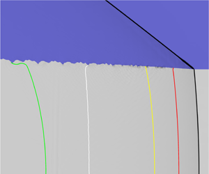
In contrast to unconfined explosives, there have been comparatively few studies on the size effect curve and failure diameter/thickness for confined charges. We know that strong confinement of the explosive significantly reduces the charge size that leads to detonation failure. This is because strong confinement limits the amount of streamline divergence in the DDZ, and thus the degree of energy losses to which the detonation is subjected. The most detailed, relevant study on this effect is that of Ramsay (Reference Ramsay1985), who examined the detonation failure thickness of PBX 9502 as a function of the impedance and thickness of the surrounding confiner. These results are summarized in figure 1. For aluminium confinement, the failure thickness decreased significantly as the confiner thickness increased, down to the order of a reaction zone thickness. For thin confinement walls of fixed width, the PBX 9502 failure thickness decreased going from aluminium to lead to copper confinement, i.e. as the impedance of the confiner increased.
The results of Ramsay (Reference Ramsay1985) for thin walls of the materials, aluminium, lead and copper suggest that, for even higher density materials, such as tantalum or platinum, the HE thickness at the failure point could be smaller than the reaction zone thickness. This conjecture motivates us to consider the dynamics of detonation propagation and failure for a problem of a strongly confined explosive (small material interface deflection angle) in which the channel width is small relative to the reaction zone length. As shown below, the consideration of this limit reveals some significant insights into the dynamics of how confinement affects both detonation propagation and failure. For all but the most sensitive of explosives, the latter requires a theory for which the detonation speed $D_{0}({<}D_{CJ})$
is such that
$D_{0}({<}D_{CJ})$
is such that $1-D_{0}/D_{CJ}=O(1),$
where
$1-D_{0}/D_{CJ}=O(1),$
where $D_{CJ}$
is the Chapman–Jouguet (CJ) detonation speed (Fickett & Davis Reference Fickett and Davis1979), with the relative departures of
$D_{CJ}$
is the Chapman–Jouguet (CJ) detonation speed (Fickett & Davis Reference Fickett and Davis1979), with the relative departures of $D_{0}$
from
$D_{0}$
from $D_{CJ}$
at the failure point increasing as the explosive becomes more non-ideal (Campbell & Engelke Reference Campbell and Engelke1976). In analogy with studies in laminar flames, we refer to this as a thick detonation limit (Daou & Matalon Reference Daou and Matalon2001; Short & Kessler Reference Short and Kessler2009; Kurdyumov & Matalon Reference Kurdyumov and Matalon2013; Pearce & Daou Reference Pearce and Daou2014; Kagan, Gordon & Sivashinsky Reference Kagan, Gordon and Sivashinsky2015).
$D_{CJ}$
at the failure point increasing as the explosive becomes more non-ideal (Campbell & Engelke Reference Campbell and Engelke1976). In analogy with studies in laminar flames, we refer to this as a thick detonation limit (Daou & Matalon Reference Daou and Matalon2001; Short & Kessler Reference Short and Kessler2009; Kurdyumov & Matalon Reference Kurdyumov and Matalon2013; Pearce & Daou Reference Pearce and Daou2014; Kagan, Gordon & Sivashinsky Reference Kagan, Gordon and Sivashinsky2015).
Figure 1. Summary of the PBX 9502 failure thickness results from Ramsay (Reference Ramsay1985).
2 Model
We consider a steady, symmetrical detonation propagating axially with constant speed $D_{0}$
in either a 2-D planar or axisymmetric cylindrical geometry, as shown in figure 2(a). The planar geometry has thickness
$D_{0}$
in either a 2-D planar or axisymmetric cylindrical geometry, as shown in figure 2(a). The planar geometry has thickness $T(=2W)$
, while the cylinder has radius
$T(=2W)$
, while the cylinder has radius $R(=W)$
. Ahead of the detonation the HE/confiner material interface lies at the fixed location
$R(=W)$
. Ahead of the detonation the HE/confiner material interface lies at the fixed location $r=W$
(figure 2
a). Upon detonation arrival, the material interface between the HE and confiner is deflected. For steady flow, and in a coordinate system travelling with the detonation shock at speed
$r=W$
(figure 2
a). Upon detonation arrival, the material interface between the HE and confiner is deflected. For steady flow, and in a coordinate system travelling with the detonation shock at speed $D_{0}$
, the material interface is stationary, and thus the material interface boundary can be considered equivalent to an HE streamline defining the edge of the deflected HE flow behind the shock. In contrast to our previous studies that have set this boundary streamline to be straight (Chiquete et al.
Reference Chiquete, Short, Meyer and Quirk2018; Chiquete, Short & Quirk Reference Chiquete, Short and Quirk2019; Chiquete & Short Reference Chiquete and Short2019), here, we assume that the shape of the streamline can be arbitrarily prescribed, thus enabling us to study the effects on detonation propagation of boundary streamline curvature. In § 6, we determine the curved HE boundary streamline (material interface) shape for a series of confinement materials via multi-material simulation.
$D_{0}$
, the material interface is stationary, and thus the material interface boundary can be considered equivalent to an HE streamline defining the edge of the deflected HE flow behind the shock. In contrast to our previous studies that have set this boundary streamline to be straight (Chiquete et al.
Reference Chiquete, Short, Meyer and Quirk2018; Chiquete, Short & Quirk Reference Chiquete, Short and Quirk2019; Chiquete & Short Reference Chiquete and Short2019), here, we assume that the shape of the streamline can be arbitrarily prescribed, thus enabling us to study the effects on detonation propagation of boundary streamline curvature. In § 6, we determine the curved HE boundary streamline (material interface) shape for a series of confinement materials via multi-material simulation.
The detonation flow is governed by the 2-D reactive Euler equations. These are written in non-dimensionalized form for general unsteady flows as
 $$\begin{eqnarray}\frac{\unicode[STIX]{x2202}\boldsymbol{y}}{\unicode[STIX]{x2202}t}+\frac{\unicode[STIX]{x2202}\boldsymbol{f}_{\boldsymbol{r}}}{\unicode[STIX]{x2202}r}+\frac{\unicode[STIX]{x2202}\boldsymbol{f}_{\boldsymbol{z}}}{\unicode[STIX]{x2202}z}=\boldsymbol{g},\end{eqnarray}$$

Figure 2. (a) Schematic of steady axial detonation propagation in either a planar 2-D geometry ( $W=T/2$
) or axisymmetric 2-D cylindrical geometry
$W=T/2$
) or axisymmetric 2-D cylindrical geometry $(W=R)$
in which the HE boundary is deflected upon arrival of the detonation shock. For analysis purposes, the
$(W=R)$
in which the HE boundary is deflected upon arrival of the detonation shock. For analysis purposes, the $(r,z)$
geometry in (a) is mapped to the shock- and deflected boundary-fitted frame
$(r,z)$
geometry in (a) is mapped to the shock- and deflected boundary-fitted frame $(\unicode[STIX]{x1D709},\unicode[STIX]{x1D702})$
as shown in (b).
$(\unicode[STIX]{x1D709},\unicode[STIX]{x1D702})$
as shown in (b).
where,
 $$\begin{eqnarray}\displaystyle \boldsymbol{y}=(\unicode[STIX]{x1D70C},\unicode[STIX]{x1D70C}u_{r},\unicode[STIX]{x1D70C}u_{z},\unicode[STIX]{x1D70C}E,\unicode[STIX]{x1D70C}\unicode[STIX]{x1D706})^{\intercal },\quad \boldsymbol{f}_{\boldsymbol{r}}=(\unicode[STIX]{x1D70C}u_{r},\unicode[STIX]{x1D70C}u_{r}^{2}+p,\unicode[STIX]{x1D70C}u_{r}u_{z},u_{r}(\unicode[STIX]{x1D70C}E+p),\unicode[STIX]{x1D70C}u_{r}\unicode[STIX]{x1D706})^{\intercal },\qquad & & \displaystyle\end{eqnarray}$$
 $$\begin{eqnarray}\displaystyle & \displaystyle \boldsymbol{f}_{\boldsymbol{z}}=(\unicode[STIX]{x1D70C}u_{z},\unicode[STIX]{x1D70C}u_{r}u_{z},\unicode[STIX]{x1D70C}u_{z}^{2}+p,u_{z}(\unicode[STIX]{x1D70C}E+p),\unicode[STIX]{x1D70C}u_{z}\unicode[STIX]{x1D706})^{\intercal }, & \displaystyle\end{eqnarray}$$
 $$\begin{eqnarray}\displaystyle & \displaystyle \boldsymbol{g}=(-s\unicode[STIX]{x1D70C}u_{r}/r,-s\unicode[STIX]{x1D70C}u_{r}^{2}/r,-s\unicode[STIX]{x1D70C}u_{r}u_{z}/r,-su_{r}(\unicode[STIX]{x1D70C}E+p)/r,\unicode[STIX]{x1D70C}\unicode[STIX]{x1D6EC}-s\unicode[STIX]{x1D70C}u_{r}\unicode[STIX]{x1D706}/r)^{\intercal }. & \displaystyle\end{eqnarray}$$
Here, $r$
and
$r$
and $z$
denote spatial coordinates perpendicular and parallel to the undeflected boundary streamline, respectively (figure 2
a),
$z$
denote spatial coordinates perpendicular and parallel to the undeflected boundary streamline, respectively (figure 2
a), $t$
is time, while
$t$
is time, while $\unicode[STIX]{x1D70C}$
,
$\unicode[STIX]{x1D70C}$
, $\boldsymbol{u}$
,
$\boldsymbol{u}$
, $E$
and
$E$
and $p$
are the density, laboratory-frame flow velocity vector, total energy and pressure, respectively. For the two-dimensional flow being considered, the velocity vector
$p$
are the density, laboratory-frame flow velocity vector, total energy and pressure, respectively. For the two-dimensional flow being considered, the velocity vector $\boldsymbol{u}=(u_{r},u_{z})^{\intercal }$
. The reaction progress variable,
$\boldsymbol{u}=(u_{r},u_{z})^{\intercal }$
. The reaction progress variable, $\unicode[STIX]{x1D706}\in [0,1]$
, tracks the conversion of reactants
$\unicode[STIX]{x1D706}\in [0,1]$
, tracks the conversion of reactants $(\unicode[STIX]{x1D706}=0)$
to products
$(\unicode[STIX]{x1D706}=0)$
to products $(\unicode[STIX]{x1D706}=1)$
at the rate
$(\unicode[STIX]{x1D706}=1)$
at the rate $\unicode[STIX]{x1D6EC}$
. The symmetry parameter
$\unicode[STIX]{x1D6EC}$
. The symmetry parameter $s=0$
for the planar geometry, while
$s=0$
for the planar geometry, while $s=1$
for the cylindrical geometry. The total energy and frozen sound speed
$s=1$
for the cylindrical geometry. The total energy and frozen sound speed $c$
are given by
$c$
are given by
 $$\begin{eqnarray}E=e(\unicode[STIX]{x1D70C},p,\unicode[STIX]{x1D706})+\frac{1}{2}(u_{r}^{2}+u_{z}^{2}),\quad c^{2}=\left(\frac{\unicode[STIX]{x2202}e}{\unicode[STIX]{x2202}p}\right)^{-1}\left(\frac{p}{\unicode[STIX]{x1D70C}^{2}}-\frac{\unicode[STIX]{x2202}e}{\unicode[STIX]{x2202}\unicode[STIX]{x1D70C}}\right),\end{eqnarray}$$
respectively, where $e$
is the internal energy. The detonation shock conditions are
$e$
is the internal energy. The detonation shock conditions are
 $$\begin{eqnarray}\left.\begin{array}{@{}c@{}}\displaystyle \unicode[STIX]{x1D70C}_{s}(u_{n,s}-D_{n,s})=-\unicode[STIX]{x1D70C}_{0}D_{n,s},\quad p_{s}=\unicode[STIX]{x1D70C}_{0}^{2}D_{n,s}^{2}\left({\displaystyle \frac{1}{\unicode[STIX]{x1D70C}_{0}}}-\frac{1}{\unicode[STIX]{x1D70C}_{s}}\right),\\ e_{s}-e_{0}={\displaystyle \frac{1}{2}}p_{s}\left({\displaystyle \frac{1}{\unicode[STIX]{x1D70C}_{0}}}-{\displaystyle \frac{1}{\unicode[STIX]{x1D70C}_{s}}}\right),\quad \unicode[STIX]{x1D706}_{s}=0,\quad u_{t,s}=0,\end{array}\right\}\end{eqnarray}$$
where $u_{t,s}$
and
$u_{t,s}$
and $u_{n,s}$
are the tangential and normal flow speeds at the shock,
$u_{n,s}$
are the tangential and normal flow speeds at the shock, $D_{n,s}$
is the shock speed in the shock normal direction and
$D_{n,s}$
is the shock speed in the shock normal direction and $\unicode[STIX]{x1D70C}_{0}$
and
$\unicode[STIX]{x1D70C}_{0}$
and $e_{0}$
are the density and internal energy of the unshocked reactant material, respectively. The subscript
$e_{0}$
are the density and internal energy of the unshocked reactant material, respectively. The subscript $\{\}_{s}$
is used here to denote the shock state.
$\{\}_{s}$
is used here to denote the shock state.
The non-dimensional scaling employed above is similar to that used by Short et al. (Reference Short, Quirk, Chiquete and Meyer2018) and given by
 $$\begin{eqnarray}\left.\begin{array}{@{}c@{}}\displaystyle (r,z)={\displaystyle \frac{(\tilde{r},\tilde{z})}{\tilde{l}_{ref}}},~t={\displaystyle \frac{\tilde{t}}{(\tilde{l}_{ref}/\tilde{u} _{ref})}},~\unicode[STIX]{x1D70C}={\displaystyle \frac{\tilde{\unicode[STIX]{x1D70C}}}{\tilde{\unicode[STIX]{x1D70C}}_{ref}}},~\boldsymbol{u}={\displaystyle \frac{\tilde{\boldsymbol{u}}}{\tilde{u} _{ref}}},~p={\displaystyle \frac{\tilde{p}}{\tilde{\unicode[STIX]{x1D70C}}_{ref}\tilde{u} _{ref}^{2}}},~e={\displaystyle \frac{\tilde{e}}{\tilde{u} _{ref}^{2}}},\\ \displaystyle D_{CJ}={\displaystyle \frac{\tilde{D}_{CJ}}{\tilde{u} _{ref}}},~c={\displaystyle \frac{\tilde{c}}{\tilde{u} _{ref}}},~\end{array}\right\}\end{eqnarray}$$
where $\tilde{\{~\}}$
quantities are dimensional. However, in contrast to Short et al. (Reference Short, Quirk, Chiquete and Meyer2018), where a partial reaction length scale is used for
$\tilde{\{~\}}$
quantities are dimensional. However, in contrast to Short et al. (Reference Short, Quirk, Chiquete and Meyer2018), where a partial reaction length scale is used for $\tilde{l}_{ref}$
, for the purposes of conducting the asymptotic analysis described in § 4, we initially set the reference length scale
$\tilde{l}_{ref}$
, for the purposes of conducting the asymptotic analysis described in § 4, we initially set the reference length scale $\tilde{l}_{ref}$
to be characteristic of the total length of the DDZ, i.e. representative of the distance between the detonation shock and sonic flow boundary. We return to the discussion of
$\tilde{l}_{ref}$
to be characteristic of the total length of the DDZ, i.e. representative of the distance between the detonation shock and sonic flow boundary. We return to the discussion of $\tilde{l}_{ref}$
to best present the results of the asymptotic analysis in § 5. Also, we take
$\tilde{l}_{ref}$
to best present the results of the asymptotic analysis in § 5. Also, we take $\tilde{u} _{ref}=1~\text{mm}~\unicode[STIX]{x03BC}\text{s}^{-1}$
and
$\tilde{u} _{ref}=1~\text{mm}~\unicode[STIX]{x03BC}\text{s}^{-1}$
and $\tilde{\unicode[STIX]{x1D70C}}_{ref}=1~\text{g}~\text{cm}^{-3}$
as in Short et al. (Reference Short, Quirk, Chiquete and Meyer2018).
$\tilde{\unicode[STIX]{x1D70C}}_{ref}=1~\text{g}~\text{cm}^{-3}$
as in Short et al. (Reference Short, Quirk, Chiquete and Meyer2018).
3 Shock- and boundary streamline-attached frame
We are concerned with steady flows, and to facilitate the analysis, coordinates $r$
and
$r$
and $z$
are transformed according to
$z$
are transformed according to
 $$\begin{eqnarray}r(\unicode[STIX]{x1D709},\unicode[STIX]{x1D702})=\left(1-\frac{m_{e}h(\unicode[STIX]{x1D702})}{W}\right)\unicode[STIX]{x1D709},\quad z(\unicode[STIX]{x1D709},\unicode[STIX]{x1D702})=D_{0}t+z_{s}(\unicode[STIX]{x1D709})+\unicode[STIX]{x1D702},\end{eqnarray}$$
assuming that ahead of the detonation shock front the HE boundary streamline (material interface) lies at $r=W.$
The HE boundary streamline shape as a function of
$r=W.$
The HE boundary streamline shape as a function of $\unicode[STIX]{x1D702}({\leqslant}0)$
is given by
$\unicode[STIX]{x1D702}({\leqslant}0)$
is given by $-m_{e}h(\unicode[STIX]{x1D702}),h(0)=0,$
with
$-m_{e}h(\unicode[STIX]{x1D702}),h(0)=0,$
with $m_{e}$
representing the magnitude of the boundary streamline gradient at
$m_{e}$
representing the magnitude of the boundary streamline gradient at $\unicode[STIX]{x1D702}=0,$
so that
$\unicode[STIX]{x1D702}=0,$
so that $h^{\prime }(0)=1.$
For the majority of cases of interest,
$h^{\prime }(0)=1.$
For the majority of cases of interest, $m_{e}>0$
and
$m_{e}>0$
and $h(\unicode[STIX]{x1D702})<0$
for
$h(\unicode[STIX]{x1D702})<0$
for $\unicode[STIX]{x1D702}<0,$
although some situations can arise where
$\unicode[STIX]{x1D702}<0,$
although some situations can arise where $m_{e}<0$
as discussed in § 6.2. In terms of the boundary streamline deflection angle
$m_{e}<0$
as discussed in § 6.2. In terms of the boundary streamline deflection angle $\unicode[STIX]{x1D703}_{e}$
(figure 2
a) at
$\unicode[STIX]{x1D703}_{e}$
(figure 2
a) at $\unicode[STIX]{x1D702}=0,$ $m_{e}=\tan \unicode[STIX]{x1D703}_{e}$
. Also,
$m_{e}=\tan \unicode[STIX]{x1D703}_{e}$
. Also, $W=T/2$
(planar) or
$W=T/2$
(planar) or $W=R$
(cylindrical), while
$W=R$
(cylindrical), while $z=z_{s}(\unicode[STIX]{x1D709})$
is the steady shock shape, aligned so that
$z=z_{s}(\unicode[STIX]{x1D709})$
is the steady shock shape, aligned so that $z_{s}(0)=0.$
The Jacobian
 $$\begin{eqnarray}|J|=\frac{\unicode[STIX]{x2202}r}{\unicode[STIX]{x2202}\unicode[STIX]{x1D709}}-\frac{\unicode[STIX]{x2202}r}{\unicode[STIX]{x2202}\unicode[STIX]{x1D702}}\frac{\unicode[STIX]{x2202}z_{s}}{\unicode[STIX]{x2202}\unicode[STIX]{x1D709}},\end{eqnarray}$$
should be positive to ensure an appropriate mapping from $(r,z)$
to
$(r,z)$
to $(\unicode[STIX]{x1D709},\unicode[STIX]{x1D702})$
. This generates the coordinate system shown in figure 2(b), where
$(\unicode[STIX]{x1D709},\unicode[STIX]{x1D702})$
. This generates the coordinate system shown in figure 2(b), where $\unicode[STIX]{x1D702}=0$
is the transformed shock position,
$\unicode[STIX]{x1D702}=0$
is the transformed shock position, $\unicode[STIX]{x1D709}=W$
is the location of the deflected streamline boundary and
$\unicode[STIX]{x1D709}=W$
is the location of the deflected streamline boundary and $\unicode[STIX]{x1D709}=0$
represents the axis of symmetry. Boundary conditions are applied along
$\unicode[STIX]{x1D709}=0$
represents the axis of symmetry. Boundary conditions are applied along $\unicode[STIX]{x1D702}=0,\unicode[STIX]{x1D709}=0$
and
$\unicode[STIX]{x1D702}=0,\unicode[STIX]{x1D709}=0$
and $\unicode[STIX]{x1D709}=W,$
thus reducing the problem to consideration of the flow domain
$\unicode[STIX]{x1D709}=W,$
thus reducing the problem to consideration of the flow domain $\unicode[STIX]{x1D702}\leqslant 0$
and
$\unicode[STIX]{x1D702}\leqslant 0$
and $0\leqslant \unicode[STIX]{x1D709}\leqslant W.$
Under (3.1), the steady version of the flow (2.1) becomes
 $$\begin{eqnarray}\frac{\unicode[STIX]{x2202}\boldsymbol{F}_{\unicode[STIX]{x1D743}}}{\unicode[STIX]{x2202}\unicode[STIX]{x1D709}}+\frac{\unicode[STIX]{x2202}\boldsymbol{F}_{\boldsymbol{\unicode[STIX]{x1D702}}}}{\unicode[STIX]{x2202}\unicode[STIX]{x1D702}}=\boldsymbol{G},\end{eqnarray}$$
where
 $$\begin{eqnarray}\boldsymbol{F}_{\unicode[STIX]{x1D743}}=\boldsymbol{f}_{\boldsymbol{r}}-\frac{\unicode[STIX]{x2202}r}{\unicode[STIX]{x2202}\unicode[STIX]{x1D702}}(\,\boldsymbol{f}_{\boldsymbol{z}}-D_{0}\,\boldsymbol{y}),\quad \boldsymbol{F}_{\boldsymbol{\unicode[STIX]{x1D702}}}=-\frac{\unicode[STIX]{x2202}z_{s}}{\unicode[STIX]{x2202}\unicode[STIX]{x1D709}}\boldsymbol{f}_{\boldsymbol{r}}+\frac{\unicode[STIX]{x2202}r}{\unicode[STIX]{x2202}\unicode[STIX]{x1D709}}(\,\boldsymbol{f}_{\boldsymbol{z}}-D_{0}\,\boldsymbol{y}),\quad \boldsymbol{G}=|J|\boldsymbol{g},\end{eqnarray}$$
and
 $$\begin{eqnarray}\frac{\unicode[STIX]{x2202}r}{\unicode[STIX]{x2202}\unicode[STIX]{x1D702}}=-\frac{\unicode[STIX]{x1D709}m_{e}}{W}h^{\prime }(\unicode[STIX]{x1D702}),\quad \frac{\unicode[STIX]{x2202}r}{\unicode[STIX]{x2202}\unicode[STIX]{x1D709}}=1-\frac{m_{e}}{W}h(\unicode[STIX]{x1D702}),\quad |J|=1-\frac{m_{e}}{W}h(\unicode[STIX]{x1D702})+\frac{\unicode[STIX]{x1D709}m_{e}}{W}h^{\prime }(\unicode[STIX]{x1D702})\frac{\unicode[STIX]{x2202}z_{s}}{\unicode[STIX]{x2202}\unicode[STIX]{x1D709}}.\end{eqnarray}$$
Symmetry conditions are applied along the central axis ( $\unicode[STIX]{x1D709}=0$
), while along the boundary streamline (
$\unicode[STIX]{x1D709}=0$
), while along the boundary streamline ( $\unicode[STIX]{x1D709}=W$
) the only condition to be applied is that the normal flow component is zero, giving
$\unicode[STIX]{x1D709}=W$
) the only condition to be applied is that the normal flow component is zero, giving
 $$\begin{eqnarray}u_{r}(\unicode[STIX]{x1D709}=0,\unicode[STIX]{x1D702})=0,\quad u_{r}(\unicode[STIX]{x1D709}=W,\unicode[STIX]{x1D702})=-m_{e}h^{\prime }(\unicode[STIX]{x1D702})(u_{z}-D_{0}).\end{eqnarray}$$
On the shock front, the flow solution is determined from the jump conditions (2.6) as a function of $D_{n,s}=D_{n,s}(\unicode[STIX]{x1D709}),$
where, from the geometric shock surface evolution,
$D_{n,s}=D_{n,s}(\unicode[STIX]{x1D709}),$
where, from the geometric shock surface evolution,
 $$\begin{eqnarray}D_{0}=D_{n,s}\sqrt{\left(\frac{\unicode[STIX]{x2202}z_{s}}{\unicode[STIX]{x2202}\unicode[STIX]{x1D709}}\right)^{2}+1}.\end{eqnarray}$$
4 Thin channel, strong confinement, asymptotic analysis
Based on the discussion in § 1, we look for strong confinement solutions in which the lateral extent of the charge is smaller than the detonation driving zone thickness, the latter of which is characterized spatially by $\unicode[STIX]{x1D702}=O(1)$
. Consequently, we set
$\unicode[STIX]{x1D702}=O(1)$
. Consequently, we set $\unicode[STIX]{x1D709}=O(\unicode[STIX]{x1D6FF}),\unicode[STIX]{x1D6FF}\ll 1,$
with
$\unicode[STIX]{x1D709}=O(\unicode[STIX]{x1D6FF}),\unicode[STIX]{x1D6FF}\ll 1,$
with $W=O(\unicode[STIX]{x1D6FF}).$
We are then left with the objective of setting a scale on the boundary streamline gradient
$W=O(\unicode[STIX]{x1D6FF}).$
We are then left with the objective of setting a scale on the boundary streamline gradient $m_{e}$
. As noted in § 1, our aim is to develop a theory that can describe detonation propagation and failure regimes in which the detonation speed
$m_{e}$
. As noted in § 1, our aim is to develop a theory that can describe detonation propagation and failure regimes in which the detonation speed $D_{0}$
departs from
$D_{0}$
departs from $D_{CJ}$
by
$D_{CJ}$
by $O(1)$
amounts, such that
$O(1)$
amounts, such that $1-D_{0}/D_{CJ}=O(1).$
In the absence of any boundary streamline deflection (
$1-D_{0}/D_{CJ}=O(1).$
In the absence of any boundary streamline deflection ( $m_{e}=0$
), the leading-order solution is a detonation wave propagating at the Chapman–Jouguet speed
$m_{e}=0$
), the leading-order solution is a detonation wave propagating at the Chapman–Jouguet speed $D_{CJ}.$
Consequently, the streamline gradient must be sufficient in magnitude so that the induced rate of change of mass flux through the detonation, and thereby the associated energy change, from the boundary streamline deflection directly influences the determination of the leading-order detonation structure, thus resulting in departures of
$D_{CJ}.$
Consequently, the streamline gradient must be sufficient in magnitude so that the induced rate of change of mass flux through the detonation, and thereby the associated energy change, from the boundary streamline deflection directly influences the determination of the leading-order detonation structure, thus resulting in departures of $D_{0}/D_{CJ}$
from one by
$D_{0}/D_{CJ}$
from one by $O(1)$
amounts. As is apparent below, this can only be achieved if the boundary streamline gradient behind the shock is similar in magnitude, asymptotically, to the lateral charge size, i.e.
$O(1)$
amounts. As is apparent below, this can only be achieved if the boundary streamline gradient behind the shock is similar in magnitude, asymptotically, to the lateral charge size, i.e. $O(\unicode[STIX]{x1D6FF})$
. Thus we also set
$O(\unicode[STIX]{x1D6FF})$
. Thus we also set $m_{e}=O(\unicode[STIX]{x1D6FF}),$
with
$m_{e}=O(\unicode[STIX]{x1D6FF}),$
with $h^{\prime }(\unicode[STIX]{x1D702})=O(1).$
Concurrently, the magnitude of the shock slope variation due to the boundary streamline deflection is
$h^{\prime }(\unicode[STIX]{x1D702})=O(1).$
Concurrently, the magnitude of the shock slope variation due to the boundary streamline deflection is $O(\unicode[STIX]{x1D6FF}).$
Consideration of other scalings on
$O(\unicode[STIX]{x1D6FF}).$
Consideration of other scalings on $m_{e}$
such that
$m_{e}$
such that $m_{e}=o(\unicode[STIX]{x1D6FF})$
, for example
$m_{e}=o(\unicode[STIX]{x1D6FF})$
, for example $m_{e}=O(\unicode[STIX]{x1D6FF}^{2})$
, would result in the leading-order solution remaining as a detonation wave propagating at speed
$m_{e}=O(\unicode[STIX]{x1D6FF}^{2})$
, would result in the leading-order solution remaining as a detonation wave propagating at speed $D_{CJ},$
and a resulting theory would only describe departures of
$D_{CJ},$
and a resulting theory would only describe departures of $D_{0}/D_{CJ}$
from one by
$D_{0}/D_{CJ}$
from one by $O(\unicode[STIX]{x1D6FF})$
amounts. This limit is not of interest for the phenomena we wish to capture in the current study. In addition, the latter weaker limit is likely to be included within the richer limit
$O(\unicode[STIX]{x1D6FF})$
amounts. This limit is not of interest for the phenomena we wish to capture in the current study. In addition, the latter weaker limit is likely to be included within the richer limit $m_{e}=O(\unicode[STIX]{x1D6FF})$
considered in this paper.
$m_{e}=O(\unicode[STIX]{x1D6FF})$
considered in this paper.
These balance arguments lead to the introduction of the scaled variables,
 $$\begin{eqnarray}\hat{\unicode[STIX]{x1D709}}=\frac{\unicode[STIX]{x1D709}}{\unicode[STIX]{x1D6FF}},\quad {\hat{W}}=\frac{W}{\unicode[STIX]{x1D6FF}},\quad \hat{m}_{e}=\frac{m_{e}}{\unicode[STIX]{x1D6FF}},\end{eqnarray}$$
so that
 $$\begin{eqnarray}r=\unicode[STIX]{x1D6FF}\left(1-\frac{\hat{m}_{e}}{{\hat{W}}}h(\unicode[STIX]{x1D702})\right)\hat{\unicode[STIX]{x1D709}},\quad z=D_{0}t+\unicode[STIX]{x1D6FF}^{2}\hat{z}_{s}+\unicode[STIX]{x1D702},\end{eqnarray}$$
giving $\unicode[STIX]{x2202}z_{s}/\unicode[STIX]{x2202}\unicode[STIX]{x1D709}=\unicode[STIX]{x1D6FF}\unicode[STIX]{x2202}\hat{z}_{s}/\unicode[STIX]{x2202}\hat{\unicode[STIX]{x1D709}},$
and
$\unicode[STIX]{x2202}z_{s}/\unicode[STIX]{x2202}\unicode[STIX]{x1D709}=\unicode[STIX]{x1D6FF}\unicode[STIX]{x2202}\hat{z}_{s}/\unicode[STIX]{x2202}\hat{\unicode[STIX]{x1D709}},$
and
 $$\begin{eqnarray}\frac{\unicode[STIX]{x2202}r}{\unicode[STIX]{x2202}\unicode[STIX]{x1D702}}=-\unicode[STIX]{x1D6FF}\frac{\hat{m}_{e}}{{\hat{W}}}h^{\prime }(\unicode[STIX]{x1D702})\hat{\unicode[STIX]{x1D709}},\quad \frac{\unicode[STIX]{x2202}r}{\unicode[STIX]{x2202}\unicode[STIX]{x1D709}}=1-\frac{\hat{m}_{e}}{{\hat{W}}}h(\unicode[STIX]{x1D702}),\quad |J|=1-\frac{\hat{m}_{e}}{{\hat{W}}}h(\unicode[STIX]{x1D702})+O(\unicode[STIX]{x1D6FF}^{2}).\end{eqnarray}$$
With this, the shock normal speed $D_{n,s}=D_{0}+O(\unicode[STIX]{x1D6FF}^{2})$
from (3.7). Balance arguments for the shock conditions and flow equations then lead us to consider
$D_{n,s}=D_{0}+O(\unicode[STIX]{x1D6FF}^{2})$
from (3.7). Balance arguments for the shock conditions and flow equations then lead us to consider $O(\unicode[STIX]{x1D6FF})$
changes in the lateral flow velocity component, and thus we define
$O(\unicode[STIX]{x1D6FF})$
changes in the lateral flow velocity component, and thus we define
 $$\begin{eqnarray}\hat{u} _{r}=\frac{u_{r}}{\unicode[STIX]{x1D6FF}}.\end{eqnarray}$$
We now seek solutions for which
 $$\begin{eqnarray}u_{z}=u_{z}^{0},\quad p=p^{0},\quad \unicode[STIX]{x1D70C}=\unicode[STIX]{x1D70C}^{0},\quad e=e^{0},\quad \unicode[STIX]{x1D706}=\unicode[STIX]{x1D706}^{0},\quad \hat{u} _{r}=\hat{u} _{r}^{1},\end{eqnarray}$$
all have $O(1)$
variation. The normal flow velocity component at the shock becomes
$O(1)$
variation. The normal flow velocity component at the shock becomes $u_{n,s}=u_{z}^{0}+O(\unicode[STIX]{x1D6FF}^{2}),$
so that, to leading order, (2.6) become
$u_{n,s}=u_{z}^{0}+O(\unicode[STIX]{x1D6FF}^{2}),$
so that, to leading order, (2.6) become
 $$\begin{eqnarray}\unicode[STIX]{x1D70C}_{s}^{0}(u_{z,s}^{0}-D_{0})=-\unicode[STIX]{x1D70C}_{0}D_{0},\quad p_{s}^{0}=\unicode[STIX]{x1D70C}_{0}^{2}D_{0}^{2}\left(\frac{1}{\unicode[STIX]{x1D70C}_{0}}-\frac{1}{\unicode[STIX]{x1D70C}_{s}^{0}}\right)\!,\quad e_{s}^{0}-e_{0}=\frac{1}{2}p_{s}^{0}\left(\frac{1}{\unicode[STIX]{x1D70C}_{0}}-\frac{1}{\unicode[STIX]{x1D70C}_{s}^{0}}\right)\!,\quad \unicode[STIX]{x1D706}_{s}^{0}=0,\end{eqnarray}$$
at $\unicode[STIX]{x1D702}=0.$
The shock tangential flow condition,
$\unicode[STIX]{x1D702}=0.$
The shock tangential flow condition, $u_{t,s}=0,$
also gives
$u_{t,s}=0,$
also gives
 $$\begin{eqnarray}\hat{u} _{r,s}^{1}=-u_{z,s}^{0}\frac{\text{d}\hat{z}_{s}}{\text{d}\hat{\unicode[STIX]{x1D709}}},\end{eqnarray}$$
while the symmetry and boundary streamline conditions (3.6) lead to
 $$\begin{eqnarray}\hat{u} _{r}^{1}(\unicode[STIX]{x1D702},\hat{\unicode[STIX]{x1D709}}=0)=0,\quad \hat{u} _{r}^{1}(\unicode[STIX]{x1D702},\hat{\unicode[STIX]{x1D709}}={\hat{W}})=-\hat{m}_{e}h^{\prime }(\unicode[STIX]{x1D702})(u_{z}^{0}-D_{0}).\end{eqnarray}$$
With the axial detonation phase speed $D_{0}$
constant for steady flows, guided by the shock relations (4.6), we now seek solutions of the scaled flow equations
$D_{0}$
constant for steady flows, guided by the shock relations (4.6), we now seek solutions of the scaled flow equations
 $$\begin{eqnarray}\frac{\unicode[STIX]{x2202}\boldsymbol{F}_{\unicode[STIX]{x1D743}}}{\unicode[STIX]{x2202}\hat{\unicode[STIX]{x1D709}}}=\unicode[STIX]{x1D6FF}\left(\boldsymbol{G}-\frac{\unicode[STIX]{x2202}\boldsymbol{F}_{\boldsymbol{\unicode[STIX]{x1D702}}}}{\unicode[STIX]{x2202}\unicode[STIX]{x1D702}}\right),\end{eqnarray}$$
for which
 $$\begin{eqnarray}u_{z}^{0}=u_{z}^{0}(\unicode[STIX]{x1D702}),\quad p^{0}=p^{0}(\unicode[STIX]{x1D702}),\quad \unicode[STIX]{x1D70C}^{0}=\unicode[STIX]{x1D70C}^{0}(\unicode[STIX]{x1D702}),\quad e^{0}=e^{0}(\unicode[STIX]{x1D702}),\quad \unicode[STIX]{x1D706}^{0}=\unicode[STIX]{x1D706}^{0}(\unicode[STIX]{x1D702}).\end{eqnarray}$$
In general, for each flow vector component, we find $\boldsymbol{F}_{\unicode[STIX]{x1D743}}=O(\unicode[STIX]{x1D6FF}),\boldsymbol{F}_{\!\boldsymbol{\unicode[STIX]{x1D702}}}=O(1)$
and
$\boldsymbol{F}_{\unicode[STIX]{x1D743}}=O(\unicode[STIX]{x1D6FF}),\boldsymbol{F}_{\!\boldsymbol{\unicode[STIX]{x1D702}}}=O(1)$
and $\boldsymbol{G}=O(1),$
with the leading-order balance for each component occurring at
$\boldsymbol{G}=O(1),$
with the leading-order balance for each component occurring at $O(\unicode[STIX]{x1D6FF})$
in (4.9).
$O(\unicode[STIX]{x1D6FF})$
in (4.9).
For the continuity equation,
 $$\begin{eqnarray}\frac{\unicode[STIX]{x2202}\hat{u} _{r}^{1}}{\unicode[STIX]{x2202}\hat{\unicode[STIX]{x1D709}}}+\frac{s\hat{u} _{r}^{1}}{\hat{\unicode[STIX]{x1D709}}}=-\frac{1}{\unicode[STIX]{x1D70C}^{0}}\left(1-\frac{\hat{m}_{e}}{{\hat{W}}}h(\unicode[STIX]{x1D702})\right)\frac{\text{d}}{\text{d}\unicode[STIX]{x1D702}}[\unicode[STIX]{x1D70C}^{0}(u_{z}^{0}-D_{0})].\end{eqnarray}$$
Integrating, and applying the symmetry condition (4.8),
 $$\begin{eqnarray}\hat{u} _{r}^{1}=-\frac{\hat{\unicode[STIX]{x1D709}}}{(1+s)\unicode[STIX]{x1D70C}^{0}}\left(1-\frac{\hat{m}_{e}}{{\hat{W}}}h(\unicode[STIX]{x1D702})\right)\frac{\text{d}}{\text{d}\unicode[STIX]{x1D702}}[\unicode[STIX]{x1D70C}^{0}(u_{z}^{0}-D_{0})],\end{eqnarray}$$
so that $\hat{u} _{r}^{1}$
increases linearly with
$\hat{u} _{r}^{1}$
increases linearly with $\hat{\unicode[STIX]{x1D709}}.$
Then, applying the boundary streamline condition (4.8) on
$\hat{\unicode[STIX]{x1D709}}.$
Then, applying the boundary streamline condition (4.8) on $\hat{u} _{r}^{1},$
 $$\begin{eqnarray}\frac{\text{d}}{\text{d}\unicode[STIX]{x1D702}}[\unicode[STIX]{x1D70C}^{0}(u_{z}^{0}-D_{0})]=(1+s)\frac{\hat{m}_{e}}{{\hat{W}}}h^{\prime }(\unicode[STIX]{x1D702})\left(1-\frac{\hat{m}_{e}}{{\hat{W}}}h(\unicode[STIX]{x1D702})\right)^{-1}\unicode[STIX]{x1D70C}^{0}(u_{z}^{0}-D_{0}),\end{eqnarray}$$
which can be integrated to give
 $$\begin{eqnarray}\unicode[STIX]{x1D70C}^{0}(u_{z}^{0}-D_{0})=-\unicode[STIX]{x1D70C}_{0}D_{0}\left(1-\frac{\hat{m}_{e}}{{\hat{W}}}h(\unicode[STIX]{x1D702})\right)^{-(1+s)},\end{eqnarray}$$
after the use of the first of the shock relations (4.6). Consequently, the boundary streamline deflection induces a $|J^{0}|^{-1-s}$
change in the mass flux magnitude through the wave relative to its shock value (
$|J^{0}|^{-1-s}$
change in the mass flux magnitude through the wave relative to its shock value ( $\unicode[STIX]{x1D70C}_{0}D_{0}$
), where
$\unicode[STIX]{x1D70C}_{0}D_{0}$
), where $|J^{0}|=1-\hat{m}_{e}h(\unicode[STIX]{x1D702})/{\hat{W}}$
. Geometrically,
$|J^{0}|=1-\hat{m}_{e}h(\unicode[STIX]{x1D702})/{\hat{W}}$
. Geometrically, $|J^{0}|$
simply represents the ratio of the modified domain width
$|J^{0}|$
simply represents the ratio of the modified domain width $r={\hat{W}}-\hat{m}_{e}h(\unicode[STIX]{x1D702})$
relative to the initial HE width
$r={\hat{W}}-\hat{m}_{e}h(\unicode[STIX]{x1D702})$
relative to the initial HE width $r={\hat{W}}$
at any
$r={\hat{W}}$
at any $\unicode[STIX]{x1D702}$
, i.e. it is a stretch factor. For
$\unicode[STIX]{x1D702}$
, i.e. it is a stretch factor. For $\hat{m}_{e}>0$
and
$\hat{m}_{e}>0$
and $h^{\prime }(\unicode[STIX]{x1D702})>0(h^{\prime }(0)=1)$
, covering the majority of boundary streamline deflection cases studied later in § 6, where
$h^{\prime }(\unicode[STIX]{x1D702})>0(h^{\prime }(0)=1)$
, covering the majority of boundary streamline deflection cases studied later in § 6, where $-\hat{m}_{e}h(\unicode[STIX]{x1D702})>0$
and increasing in magnitude with increasing distance behind the shock, the magnitude of the mass flux monotonically decreases through the wave. For such cases, a curved boundary streamline in which
$-\hat{m}_{e}h(\unicode[STIX]{x1D702})>0$
and increasing in magnitude with increasing distance behind the shock, the magnitude of the mass flux monotonically decreases through the wave. For such cases, a curved boundary streamline in which $h^{\prime }(\unicode[STIX]{x1D702})$
decreases from its shock value,
$h^{\prime }(\unicode[STIX]{x1D702})$
decreases from its shock value, $h^{\prime }(0)=1,$
leads to a lowering of the rate at which the mass flux decreases through the wave, relative to a boundary streamline deflection that is assumed straight
$h^{\prime }(0)=1,$
leads to a lowering of the rate at which the mass flux decreases through the wave, relative to a boundary streamline deflection that is assumed straight $(h^{\prime }(\unicode[STIX]{x1D702})=1)$
. For one confinement case studied in § 6.2 where
$(h^{\prime }(\unicode[STIX]{x1D702})=1)$
. For one confinement case studied in § 6.2 where $m_{e}<0,$
i.e. the boundary streamline is initially deflected into the HE, the magnitude of the mass flux monotonically increases relative to its shock value in the region behind the shock front where
$m_{e}<0,$
i.e. the boundary streamline is initially deflected into the HE, the magnitude of the mass flux monotonically increases relative to its shock value in the region behind the shock front where $h^{\prime }(\unicode[STIX]{x1D702})>0.$
Returning to (4.12), we can now write $\hat{u} _{r}^{1}$
in the form
$\hat{u} _{r}^{1}$
in the form
 $$\begin{eqnarray}\unicode[STIX]{x1D70C}^{0}\hat{u} _{r}^{1}=\unicode[STIX]{x1D70C}_{0}D_{0}\frac{\hat{m}_{e}}{{\hat{W}}}h^{\prime }(\unicode[STIX]{x1D702})\left(1-\frac{\hat{m}_{e}}{{\hat{W}}}h(\unicode[STIX]{x1D702})\right)^{-(1+s)}\hat{\unicode[STIX]{x1D709}}.\end{eqnarray}$$
With this, the tangential shock condition (4.7) gives the shock slope,
 $$\begin{eqnarray}\frac{\text{d}\hat{z}_{s}}{\text{d}\hat{\unicode[STIX]{x1D709}}}=-\frac{\hat{m}_{e}}{{\hat{W}}}\frac{\unicode[STIX]{x1D70C}_{0}D_{0}}{\unicode[STIX]{x1D70C}_{s}^{0}u_{z,s}^{0}}h^{\prime }(0)\hat{\unicode[STIX]{x1D709}},\end{eqnarray}$$
so that the shock shape is given by
 $$\begin{eqnarray}\hat{z}_{s}=-\frac{\hat{m}_{e}}{2{\hat{W}}}\frac{\unicode[STIX]{x1D70C}_{0}D_{0}}{\unicode[STIX]{x1D70C}_{s}^{0}u_{z,s}^{0}}\hat{\unicode[STIX]{x1D709}}^{2},\end{eqnarray}$$
noting that $h^{\prime }(0)=1$
and
$h^{\prime }(0)=1$
and $\hat{z}_{s}(0)=0$
by definition. With the aid of (4.12) and (4.14), the leading-order axial momentum equation results in
$\hat{z}_{s}(0)=0$
by definition. With the aid of (4.12) and (4.14), the leading-order axial momentum equation results in
 $$\begin{eqnarray}\frac{\text{d}p^{0}}{\text{d}\unicode[STIX]{x1D702}}-\unicode[STIX]{x1D70C}_{0}D_{0}\left(1-\frac{\hat{m}_{e}}{{\hat{W}}}h(\unicode[STIX]{x1D702})\right)^{-(1+s)}\frac{\text{d}u_{z}^{0}}{\text{d}\unicode[STIX]{x1D702}}=0,\end{eqnarray}$$
with the leading-order rate equation resulting in
 $$\begin{eqnarray}\unicode[STIX]{x1D70C}_{0}D_{0}\left(1-\frac{\hat{m}_{e}}{{\hat{W}}}h(\unicode[STIX]{x1D702})\right)^{-(1+s)}\frac{\text{d}\unicode[STIX]{x1D706}^{0}}{\text{d}\unicode[STIX]{x1D702}}=-\unicode[STIX]{x1D70C}^{0}\unicode[STIX]{x1D6EC}.\end{eqnarray}$$
Consideration of the energy equation remains to close the system. After using (4.12), the leading-order energy equation results in
 $$\begin{eqnarray}\unicode[STIX]{x1D70C}^{0}(u_{z}^{0}-D_{0})\frac{\text{d}E^{0}}{\text{d}\unicode[STIX]{x1D702}}+\frac{\text{d}}{\text{d}\unicode[STIX]{x1D702}}(p^{0}u_{z}^{0})-\frac{p^{0}}{\unicode[STIX]{x1D70C}^{0}}\frac{\text{d}}{\text{d}\unicode[STIX]{x1D702}}[\unicode[STIX]{x1D70C}^{0}(u_{z}^{0}-D_{0})]=0.\end{eqnarray}$$
Noting that $E=e+((u_{z}^{0})^{2}+\unicode[STIX]{x1D6FF}^{2}(\hat{u} _{r}^{1})^{2})/2,$
and
$E=e+((u_{z}^{0})^{2}+\unicode[STIX]{x1D6FF}^{2}(\hat{u} _{r}^{1})^{2})/2,$
and $\text{d}e/\text{d}\unicode[STIX]{x1D702}=e_{,p}\,\text{d}p/\text{d}\unicode[STIX]{x1D702}+e_{,\unicode[STIX]{x1D70C}}\,\text{d}\unicode[STIX]{x1D70C}/\text{d}\unicode[STIX]{x1D702}+e_{,\unicode[STIX]{x1D706}}\text{d}\unicode[STIX]{x1D706}/\text{d}\unicode[STIX]{x1D702},$
where
$\text{d}e/\text{d}\unicode[STIX]{x1D702}=e_{,p}\,\text{d}p/\text{d}\unicode[STIX]{x1D702}+e_{,\unicode[STIX]{x1D70C}}\,\text{d}\unicode[STIX]{x1D70C}/\text{d}\unicode[STIX]{x1D702}+e_{,\unicode[STIX]{x1D706}}\text{d}\unicode[STIX]{x1D706}/\text{d}\unicode[STIX]{x1D702},$
where $\{~\}_{,p}=\unicode[STIX]{x2202}\{~\}/\unicode[STIX]{x2202}p$
etc., and then using (4.14), (4.18) and (4.19) to eliminate
$\{~\}_{,p}=\unicode[STIX]{x2202}\{~\}/\unicode[STIX]{x2202}p$
etc., and then using (4.14), (4.18) and (4.19) to eliminate $\text{d}p^{0}/\text{d}\unicode[STIX]{x1D702},\text{d}\unicode[STIX]{x1D70C}^{0}/\text{d}\unicode[STIX]{x1D702}$
and
$\text{d}p^{0}/\text{d}\unicode[STIX]{x1D702},\text{d}\unicode[STIX]{x1D70C}^{0}/\text{d}\unicode[STIX]{x1D702}$
and $\text{d}\unicode[STIX]{x1D706}^{0}/\text{d}\unicode[STIX]{x1D702},$
we can rewrite the energy equation (4.20) with the only derivatives in
$\text{d}\unicode[STIX]{x1D706}^{0}/\text{d}\unicode[STIX]{x1D702},$
we can rewrite the energy equation (4.20) with the only derivatives in $\unicode[STIX]{x1D702}$
associated with
$\unicode[STIX]{x1D702}$
associated with $u_{z}^{0},$
 $$\begin{eqnarray}[(c^{0})^{2}-(u_{z}^{0}-D_{0})^{2}]\frac{\text{d}u_{z}^{0}}{\text{d}\unicode[STIX]{x1D702}}=-\frac{\text{e}_{,\unicode[STIX]{x1D706}}^{0}}{\unicode[STIX]{x1D70C}^{0}\text{e}_{,p}^{0}}\unicode[STIX]{x1D6EC}-\frac{(c^{0})^{2}}{\unicode[STIX]{x1D70C}^{0}}\unicode[STIX]{x1D70C}_{0}D_{0}(1+s)\left[1-\frac{\hat{m}_{e}}{{\hat{W}}}h(\unicode[STIX]{x1D702})\right]^{-(2+s)}\frac{\hat{m}_{e}}{{\hat{W}}}h^{\prime }(\unicode[STIX]{x1D702}).\end{eqnarray}$$
Equations (4.14), (4.18), (4.19) and (4.21) are solved subject to shock relations (4.6) at $\unicode[STIX]{x1D702}=0.$
An implication of (4.21) is that the system contains a saddle point when the axial flow becomes sonic, i.e. when
$\unicode[STIX]{x1D702}=0.$
An implication of (4.21) is that the system contains a saddle point when the axial flow becomes sonic, i.e. when $(u_{z}^{0}-D_{0})^{2}=(c^{0})^{2}.$
This equates to an eigenvalue problem for the detonation phase speed
$(u_{z}^{0}-D_{0})^{2}=(c^{0})^{2}.$
This equates to an eigenvalue problem for the detonation phase speed $D_{0},$
such that any trajectory passing through the sonic flow saddle point, subject to (4.6), must involve the cancellation of the two terms on the right-hand side of (4.21) at the saddle point. For specific choices of the reaction rate and equation of state (see § 5), this would typically necessitate the use of a shooting method, iterating on
$D_{0},$
such that any trajectory passing through the sonic flow saddle point, subject to (4.6), must involve the cancellation of the two terms on the right-hand side of (4.21) at the saddle point. For specific choices of the reaction rate and equation of state (see § 5), this would typically necessitate the use of a shooting method, iterating on $D_{0}$
until the appropriate trajectory for
$D_{0}$
until the appropriate trajectory for $u_{z}^{0}(\unicode[STIX]{x1D702})$
is found that can pass through the saddle. Of particular significance in (4.14), (4.18), (4.19) and (4.21) is that, for any fixed streamline deflection component
$u_{z}^{0}(\unicode[STIX]{x1D702})$
is found that can pass through the saddle. Of particular significance in (4.14), (4.18), (4.19) and (4.21) is that, for any fixed streamline deflection component $h(\unicode[STIX]{x1D702}),$
the solution depends only on the ratio
$h(\unicode[STIX]{x1D702}),$
the solution depends only on the ratio $\hat{m}_{e}/{\hat{W}}.$
Thus once one thickness effect curve (
$\hat{m}_{e}/{\hat{W}}.$
Thus once one thickness effect curve ( $D_{0}$
versus
$D_{0}$
versus $\hat{m}_{e}/{\hat{W}}$
) has been calculated, for example for varying
$\hat{m}_{e}/{\hat{W}}$
) has been calculated, for example for varying $\hat{m}_{e}$
at fixed
$\hat{m}_{e}$
at fixed ${\hat{W}}$
, the variation is known for all
${\hat{W}}$
, the variation is known for all ${\hat{W}}.$
Physically, the left-hand side of (4.21) is related to the longitudinal propagation and advection of acoustic and kinetic energy. The first term on the right-hand side represents an energy deposition due to chemical reaction that serves to accelerate the longitudinal flow from a subsonic state immediately behind the shock to a downstream sonic state. It is always positive for an irreversible reaction. The second term on the right-hand side of (4.21) is an energy contribution resulting from the effects of the boundary streamline deflection, specifically the induced rate of change of mass flux through the wave (this term can alternatively be written as $+((c^{0})^{2}/\unicode[STIX]{x1D70C}^{0})~\text{d}/\text{d}\unicode[STIX]{x1D702}[\unicode[STIX]{x1D70C}^{0}(u_{z}^{0}-D_{0})].$
It serves to either counteract or reinforce the acceleration of longitudinal flow depending on the sign of the gradient of the streamline deflection,
$+((c^{0})^{2}/\unicode[STIX]{x1D70C}^{0})~\text{d}/\text{d}\unicode[STIX]{x1D702}[\unicode[STIX]{x1D70C}^{0}(u_{z}^{0}-D_{0})].$
It serves to either counteract or reinforce the acceleration of longitudinal flow depending on the sign of the gradient of the streamline deflection, $-m_{e}h^{\prime }(\unicode[STIX]{x1D702}).$
For
$-m_{e}h^{\prime }(\unicode[STIX]{x1D702}).$
For $m_{e}>0$
and
$m_{e}>0$
and $h^{\prime }(\unicode[STIX]{x1D702})>0,$
i.e. where the boundary streamline moves outward, the term is negative and thus serves to reduce the energy available to drive the longitudinal flow acceleration. The larger the magnitude of the streamline deflection, the greater the associated energy loss, consequently reducing the magnitude of the eigenvalue solution
$h^{\prime }(\unicode[STIX]{x1D702})>0,$
i.e. where the boundary streamline moves outward, the term is negative and thus serves to reduce the energy available to drive the longitudinal flow acceleration. The larger the magnitude of the streamline deflection, the greater the associated energy loss, consequently reducing the magnitude of the eigenvalue solution $D_{0}.$
As will be seen in § 6, for too large an energy loss, there is no eigenvalue solution for
$D_{0}.$
As will be seen in § 6, for too large an energy loss, there is no eigenvalue solution for $D_{0},$
corresponding to the loss of steady flow solutions. For
$D_{0},$
corresponding to the loss of steady flow solutions. For $m_{e}<0,$
where the boundary streamline deflection is inward at least initially, i.e. when
$m_{e}<0,$
where the boundary streamline deflection is inward at least initially, i.e. when $-m_{e}h^{\prime }(\unicode[STIX]{x1D702})>0$
, the rate of change of mass flux is positive, an effect which supports the longitudinal acceleration of the flow. As will be seen in § 6, this latter scenario can result in the eigenvalue solution
$-m_{e}h^{\prime }(\unicode[STIX]{x1D702})>0$
, the rate of change of mass flux is positive, an effect which supports the longitudinal acceleration of the flow. As will be seen in § 6, this latter scenario can result in the eigenvalue solution $D_{0}$
rising above
$D_{0}$
rising above $D_{CJ}.$
Finally, based on the form of the energy change resulting from the boundary streamline deflection, being proportional to
$D_{CJ}.$
Finally, based on the form of the energy change resulting from the boundary streamline deflection, being proportional to $h^{\prime }(\unicode[STIX]{x1D702})$
, we expect that curvature of the boundary streamline will play a significant role in determining the detonation propagation and failure properties.
$h^{\prime }(\unicode[STIX]{x1D702})$
, we expect that curvature of the boundary streamline will play a significant role in determining the detonation propagation and failure properties.
4.1 HE streamlines shapes
After specifying the boundary streamline shape, the steady flow streamline paths within the HE region can also be calculated. To leading order these are determined by
 $$\begin{eqnarray}\frac{\text{d}r}{\text{d}\unicode[STIX]{x1D702}}=\unicode[STIX]{x1D6FF}\frac{\hat{u} _{r}^{1}}{u_{z}^{0}-D_{0}}=-\frac{\hat{m}_{e}}{{\hat{W}}}h^{\prime }(\unicode[STIX]{x1D702})\left[1-\frac{\hat{m}_{e}}{{\hat{W}}}h(\unicode[STIX]{x1D702})\right]^{-1}r,\end{eqnarray}$$
after using (4.14) and (4.15). Integrating gives
 $$\begin{eqnarray}r=\unicode[STIX]{x1D6FF}\unicode[STIX]{x1D6FC}{\hat{W}}\left(1-\frac{\hat{m}_{e}}{{\hat{W}}}h(\unicode[STIX]{x1D702})\right),\quad \frac{\text{d}r}{\text{d}\unicode[STIX]{x1D702}}=-\unicode[STIX]{x1D6FF}\unicode[STIX]{x1D6FC}\hat{m}_{e}h^{\prime }(\unicode[STIX]{x1D702}),\end{eqnarray}$$
with $\unicode[STIX]{x1D6FC}(0\leqslant \unicode[STIX]{x1D6FC}\leqslant 1)$
signifying the streamline label. The symmetry line
$\unicode[STIX]{x1D6FC}(0\leqslant \unicode[STIX]{x1D6FC}\leqslant 1)$
signifying the streamline label. The symmetry line $r=0$
is a streamline, with the streamline gradient along the shock
$r=0$
is a streamline, with the streamline gradient along the shock $(\unicode[STIX]{x1D702}=0)$
increasing from the symmetry line to the boundary. The gradient of a given HE streamline at any
$(\unicode[STIX]{x1D702}=0)$
increasing from the symmetry line to the boundary. The gradient of a given HE streamline at any $\unicode[STIX]{x1D702}$
is a fixed multiple of the corresponding boundary streamline gradient. Consequently, the HE streamlines bend toward the symmetry axis if the boundary streamline also bends in that direction (§ 6.2).
$\unicode[STIX]{x1D702}$
is a fixed multiple of the corresponding boundary streamline gradient. Consequently, the HE streamlines bend toward the symmetry axis if the boundary streamline also bends in that direction (§ 6.2).
5 Equation of state and reaction rate models
The analysis above is valid for any equation of state (EOS) and reaction rate law. We now present results for both the ideal and stiffened condensed-phase detonation models (Short, Bdzil & Anguelova Reference Short, Bdzil and Anguelova2006; Short et al.
Reference Short, Anguelova, Aslam, Bdzil, Henrick and Sharpe2008), whereupon the EOS model for the internal energy, $e$
, the specific reaction enthalpy of the HE,
$e$
, the specific reaction enthalpy of the HE, $q(=\tilde{q}/\tilde{u} _{ref}^{2})$
, and frozen sound speed,
$q(=\tilde{q}/\tilde{u} _{ref}^{2})$
, and frozen sound speed, $c$
, are given by
$c$
, are given by
 $$\begin{eqnarray}e=\frac{p+A}{(\unicode[STIX]{x1D6FE}-1)\unicode[STIX]{x1D70C}}-q\unicode[STIX]{x1D706},\quad q=\frac{D_{CJ}^{2}}{2(\unicode[STIX]{x1D6FE}^{2}-1)}\left(1-\frac{A}{\unicode[STIX]{x1D70C}_{0}D_{CJ}^{2}}\right)^{2},\quad c=\left[\frac{\unicode[STIX]{x1D6FE}p+A}{\unicode[STIX]{x1D70C}}\right]^{1/2},\end{eqnarray}$$
respectively, where $\unicode[STIX]{x1D6FE}$
is the adiabatic exponent,
$\unicode[STIX]{x1D6FE}$
is the adiabatic exponent, $A$
is the stiffened constant and, as before,
$A$
is the stiffened constant and, as before, $\unicode[STIX]{x1D70C}_{0}$
is the initial density of the HE and
$\unicode[STIX]{x1D70C}_{0}$
is the initial density of the HE and $D_{CJ}$
is the Chapman–Jouguet speed. The ideal condensed-phase model (Short et al.
Reference Short, Anguelova, Aslam, Bdzil, Henrick and Sharpe2008; Chiquete & Short Reference Chiquete and Short2019) is recovered by setting
$D_{CJ}$
is the Chapman–Jouguet speed. The ideal condensed-phase model (Short et al.
Reference Short, Anguelova, Aslam, Bdzil, Henrick and Sharpe2008; Chiquete & Short Reference Chiquete and Short2019) is recovered by setting $A=0.$
Having
$A=0.$
Having $A>0$
allows for a non-zero sound speed in the unshocked explosive (Short & Quirk Reference Short and Quirk2018b
), since the initial pressure
$A>0$
allows for a non-zero sound speed in the unshocked explosive (Short & Quirk Reference Short and Quirk2018b
), since the initial pressure $p_{0}=0$
. The parameter
$p_{0}=0$
. The parameter $A$
mimics the effects of molecular attraction in solid- or liquid-state matter (Le Métayer & Saurel Reference Le Métayer and Saurel2016). The required partial derivatives of
$A$
mimics the effects of molecular attraction in solid- or liquid-state matter (Le Métayer & Saurel Reference Le Métayer and Saurel2016). The required partial derivatives of $e$
in (5.1) are
$e$
in (5.1) are
 $$\begin{eqnarray}e_{,p}=\frac{1}{(\unicode[STIX]{x1D6FE}-1)\unicode[STIX]{x1D70C}},\quad e_{,\unicode[STIX]{x1D706}}=-q.\end{eqnarray}$$
The reaction rate, $\unicode[STIX]{x1D6EC}$
, is pressure dependent and given by
$\unicode[STIX]{x1D6EC}$
, is pressure dependent and given by
 $$\begin{eqnarray}\unicode[STIX]{x1D6EC}=kp^{n}(1-\unicode[STIX]{x1D706})^{\unicode[STIX]{x1D708}},\end{eqnarray}$$
where $k$
is a rate constant,
$k$
is a rate constant, $n$
is the pressure exponent and
$n$
is the pressure exponent and $\unicode[STIX]{x1D708}$
is a reaction-order variable. Variations of the above model have been used to study the flow physics of a variety of detonation confinement problems, e.g. Bdzil (Reference Bdzil1981), Sharpe & Braithwaite (Reference Sharpe and Braithwaite2005), Short et al. (Reference Short, Quirk, Chiquete and Meyer2018) and Short & Quirk (Reference Short and Quirk2018a
,Reference Short and Quirk
b
). The model has consistently captured the primary detonation flow physics that are present when more complex equation- of state and reaction rate models are used. The fixed model parameter choices are (Short & Quirk Reference Short and Quirk2018b
; Short et al.
Reference Short, Quirk, Chiquete and Meyer2018; Chiquete & Short Reference Chiquete and Short2019)
$\unicode[STIX]{x1D708}$
is a reaction-order variable. Variations of the above model have been used to study the flow physics of a variety of detonation confinement problems, e.g. Bdzil (Reference Bdzil1981), Sharpe & Braithwaite (Reference Sharpe and Braithwaite2005), Short et al. (Reference Short, Quirk, Chiquete and Meyer2018) and Short & Quirk (Reference Short and Quirk2018a
,Reference Short and Quirk
b
). The model has consistently captured the primary detonation flow physics that are present when more complex equation- of state and reaction rate models are used. The fixed model parameter choices are (Short & Quirk Reference Short and Quirk2018b
; Short et al.
Reference Short, Quirk, Chiquete and Meyer2018; Chiquete & Short Reference Chiquete and Short2019)
 $$\begin{eqnarray}\unicode[STIX]{x1D70C}_{0}=2,\quad D_{CJ}=8,\quad \unicode[STIX]{x1D6FE}=3.\end{eqnarray}$$
Below, we explore the detonation dynamics for changes in $A$
,
$A$
, $n$
and
$n$
and $\unicode[STIX]{x1D708}.$
Finally, for the ideal and stiffened models, the shock conditions (4.6) become
$\unicode[STIX]{x1D708}.$
Finally, for the ideal and stiffened models, the shock conditions (4.6) become
 $$\begin{eqnarray}\left.\begin{array}{@{}c@{}}u_{z,s}^{0}={\displaystyle \frac{2D_{0}}{\unicode[STIX]{x1D6FE}+1}}\left(1-{\displaystyle \frac{A}{\unicode[STIX]{x1D70C}_{0}D_{0}^{2}}}\right),\quad p_{s}^{0}=2{\displaystyle \frac{\unicode[STIX]{x1D70C}_{0}D_{0}^{2}}{\unicode[STIX]{x1D6FE}+1}}\left(1-{\displaystyle \frac{A}{\unicode[STIX]{x1D70C}_{0}D_{0}^{2}}}\right),\\ \unicode[STIX]{x1D70C}_{s}^{0}=(\unicode[STIX]{x1D6FE}+1)\unicode[STIX]{x1D70C}_{0}\left[\unicode[STIX]{x1D6FE}-1+{\displaystyle \frac{2A}{\unicode[STIX]{x1D70C}_{0}D_{0}^{2}}}\right]^{-1},\quad \unicode[STIX]{x1D706}_{s}^{0}=0.\end{array}\right\}\end{eqnarray}$$
With (5.1) and (5.2), the energy equation (4.21) becomes
 $$\begin{eqnarray}[(c^{0})^{2}-(u_{z}^{0}-D_{0})^{2}]\frac{\text{d}u_{z}^{0}}{\text{d}\unicode[STIX]{x1D702}}=(\unicode[STIX]{x1D6FE}-1)q\unicode[STIX]{x1D6EC}-\frac{(c^{0})^{2}}{\unicode[STIX]{x1D70C}^{0}}\unicode[STIX]{x1D70C}_{0}D_{0}(1+s)\left[1-\frac{m_{e}}{W}h(\unicode[STIX]{x1D702})\right]^{-(2+s)}\frac{m_{e}}{W}h^{\prime }(\unicode[STIX]{x1D702}).\end{eqnarray}$$
Thus, the chemical energy deposition term, $(\unicode[STIX]{x1D6FE}-1)q\unicode[STIX]{x1D6EC},$
only varies with the reaction rate for constant
$(\unicode[STIX]{x1D6FE}-1)q\unicode[STIX]{x1D6EC},$
only varies with the reaction rate for constant $\unicode[STIX]{x1D6FE}$
and
$\unicode[STIX]{x1D6FE}$
and $q$
. Also, we have, without loss of generality, reverted to the use of the unscaled quantities
$q$
. Also, we have, without loss of generality, reverted to the use of the unscaled quantities $m_{e}=\unicode[STIX]{x1D6FF}\hat{m}_{e}$
and
$m_{e}=\unicode[STIX]{x1D6FF}\hat{m}_{e}$
and $W=\unicode[STIX]{x1D6FF}{\hat{W}}$
, where
$W=\unicode[STIX]{x1D6FF}{\hat{W}}$
, where $m_{e}$
and
$m_{e}$
and $W$
represent physically measurable quantities. For the purposes of discussion in § 6, we now write (5.6) in the form
$W$
represent physically measurable quantities. For the purposes of discussion in § 6, we now write (5.6) in the form
 $$\begin{eqnarray}\left.\begin{array}{@{}c@{}}\unicode[STIX]{x1D714}{\displaystyle \frac{\text{d}u_{z}^{0}}{\text{d}\unicode[STIX]{x1D702}}}=(\unicode[STIX]{x1D6FE}-1)q\unicode[STIX]{x1D6EC}-\unicode[STIX]{x1D70E},\quad \unicode[STIX]{x1D714}=(c^{0})^{2}-(u_{z}^{0}-D_{0})^{2},\\ \unicode[STIX]{x1D70E}={\displaystyle \frac{(c^{0})^{2}}{\unicode[STIX]{x1D70C}^{0}}}\unicode[STIX]{x1D70C}_{0}D_{0}(1+s)\left[1-{\displaystyle \frac{m_{e}}{W}}h(\unicode[STIX]{x1D702})\right]^{-(2+s)}{\displaystyle \frac{m_{e}}{W}}h^{\prime }(\unicode[STIX]{x1D702}),\end{array}\right\}\end{eqnarray}$$
where $\unicode[STIX]{x1D714}$
is a sonic flow parameter and
$\unicode[STIX]{x1D714}$
is a sonic flow parameter and $\unicode[STIX]{x1D70E}$
is the energy change associated with the rate of change of mass flux through the detonation. The detonation speed eigenvalue
$\unicode[STIX]{x1D70E}$
is the energy change associated with the rate of change of mass flux through the detonation. The detonation speed eigenvalue $D_{0}$
for the asymptotically derived system (5.7), given any geometry parameters
$D_{0}$
for the asymptotically derived system (5.7), given any geometry parameters $s$
and
$s$
and $W$
and confinement conditions specified by
$W$
and confinement conditions specified by $m_{e}$
and
$m_{e}$
and $h(\unicode[STIX]{x1D702})$
, is determined by a shooting method similar to that described in § 4. Specifically, we make an initial guess for the eigenvalue
$h(\unicode[STIX]{x1D702})$
, is determined by a shooting method similar to that described in § 4. Specifically, we make an initial guess for the eigenvalue $D_{0}.$
With that
$D_{0}.$
With that $D_{0}$
, the shock condition at
$D_{0}$
, the shock condition at $\unicode[STIX]{x1D702}=0$
for
$\unicode[STIX]{x1D702}=0$
for $u_{z}^{0}$
is given by (5.5), whereupon the ordinary differential equation for
$u_{z}^{0}$
is given by (5.5), whereupon the ordinary differential equation for $u_{z}^{0}(\unicode[STIX]{x1D702})$
, given by (5.7), is integrated numerically. Note that this also requires the determination of
$u_{z}^{0}(\unicode[STIX]{x1D702})$
, given by (5.7), is integrated numerically. Note that this also requires the determination of $p^{0}(\unicode[STIX]{x1D702}),\unicode[STIX]{x1D70C}^{0}(\unicode[STIX]{x1D702})$
and
$p^{0}(\unicode[STIX]{x1D702}),\unicode[STIX]{x1D70C}^{0}(\unicode[STIX]{x1D702})$
and $\unicode[STIX]{x1D706}^{0}(\unicode[STIX]{x1D702})$
obtained from the simultaneous integration of (4.18) and (4.19) and the use of (4.14). The eigenvalue
$\unicode[STIX]{x1D706}^{0}(\unicode[STIX]{x1D702})$
obtained from the simultaneous integration of (4.18) and (4.19) and the use of (4.14). The eigenvalue $D_{0}$
is then iterated on until the (positive) rate term
$D_{0}$
is then iterated on until the (positive) rate term $(\unicode[STIX]{x1D6FE}-1)q\unicode[STIX]{x1D6EC}$
and (negative) energy change term
$(\unicode[STIX]{x1D6FE}-1)q\unicode[STIX]{x1D6EC}$
and (negative) energy change term $\unicode[STIX]{x1D70E}$
exactly cancel at the sonic flow point (
$\unicode[STIX]{x1D70E}$
exactly cancel at the sonic flow point ( $\unicode[STIX]{x1D714}=0$
), allowing the trajectory for
$\unicode[STIX]{x1D714}=0$
), allowing the trajectory for $u_{z}^{0}(\unicode[STIX]{x1D702})$
to pass through the saddle point.
$u_{z}^{0}(\unicode[STIX]{x1D702})$
to pass through the saddle point.
It remains to set the reference length scale that we will use for clarity of presentation of the asymptotic results. In § 6, we will set $\tilde{l}_{ref}$
to be the familiar and standard choice for detonation propagation studies, namely
$\tilde{l}_{ref}$
to be the familiar and standard choice for detonation propagation studies, namely $\tilde{l}_{ref}=\tilde{l}_{1/2}$
is the length over which 50 % of the reactants are consumed in the 1-D, steady, CJ wave (Short & Quirk Reference Short and Quirk2018b
). This has the benefit that
$\tilde{l}_{ref}=\tilde{l}_{1/2}$
is the length over which 50 % of the reactants are consumed in the 1-D, steady, CJ wave (Short & Quirk Reference Short and Quirk2018b
). This has the benefit that $\tilde{l}_{1/2}$
varies only with the model parameters choices
$\tilde{l}_{1/2}$
varies only with the model parameters choices $A$
,
$A$
, $n$
and
$n$
and $\unicode[STIX]{x1D708}$
for fixed
$\unicode[STIX]{x1D708}$
for fixed $\unicode[STIX]{x1D70C}_{0},D_{CJ}$
and
$\unicode[STIX]{x1D70C}_{0},D_{CJ}$
and $\unicode[STIX]{x1D6FE}.$
Significantly,
$\unicode[STIX]{x1D6FE}.$
Significantly, $\tilde{l}_{1/2}$
does not vary with changes in the channel width. Adopting this scale, the channel width
$\tilde{l}_{1/2}$
does not vary with changes in the channel width. Adopting this scale, the channel width $W$
appearing in (5.7) now becomes
$W$
appearing in (5.7) now becomes $W=\tilde{W}/\tilde{l}_{1/2}$
, so that
$W=\tilde{W}/\tilde{l}_{1/2}$
, so that $W$
is always referenced relative to a fixed scale. The downside of using
$W$
is always referenced relative to a fixed scale. The downside of using $\tilde{l}_{1/2}$
as the reference length is that it does not reflect the changes in overall reaction zone length that occur when the detonation speed
$\tilde{l}_{1/2}$
as the reference length is that it does not reflect the changes in overall reaction zone length that occur when the detonation speed $D_{0}$
drops below
$D_{0}$
drops below $D_{CJ}$
as a result of varying
$D_{CJ}$
as a result of varying $m_{e}$
or
$m_{e}$
or $W$
(as seen in § 6). The second alternative reference length scale
$W$
(as seen in § 6). The second alternative reference length scale $\tilde{l}_{ref}=\tilde{l}_{\unicode[STIX]{x1D702}_{s}}$
, more naturally suited to the development of the asymptotic analysis in § 4, is set to the length between the detonation shock and flow sonic point for each HE boundary streamline deflection case such that the position of the sonic flow point (§ 4) is always at
$\tilde{l}_{ref}=\tilde{l}_{\unicode[STIX]{x1D702}_{s}}$
, more naturally suited to the development of the asymptotic analysis in § 4, is set to the length between the detonation shock and flow sonic point for each HE boundary streamline deflection case such that the position of the sonic flow point (§ 4) is always at $\unicode[STIX]{x1D702}=-1$
. We will denote the channel width relative to this scale as
$\unicode[STIX]{x1D702}=-1$
. We will denote the channel width relative to this scale as $W_{\unicode[STIX]{x1D702}_{s}}$
. The scaling between
$W_{\unicode[STIX]{x1D702}_{s}}$
. The scaling between $W(=\tilde{W}/\tilde{l}_{1/2})$
and
$W(=\tilde{W}/\tilde{l}_{1/2})$
and $W_{\unicode[STIX]{x1D702}_{s}}(=\tilde{W}/\tilde{l}_{\unicode[STIX]{x1D702}_{s}})$
is determined by the ratio of the two reference length scales, i.e.
$W_{\unicode[STIX]{x1D702}_{s}}(=\tilde{W}/\tilde{l}_{\unicode[STIX]{x1D702}_{s}})$
is determined by the ratio of the two reference length scales, i.e. $W=(\tilde{W}/\tilde{l}_{\unicode[STIX]{x1D702}_{s}})(\tilde{l}_{\unicode[STIX]{x1D702}_{s}}/\tilde{l}_{1/2})=W_{\unicode[STIX]{x1D702}_{s}}(\tilde{l}_{\unicode[STIX]{x1D702}_{s}}/\tilde{l}_{1/2})$
. Since
$W=(\tilde{W}/\tilde{l}_{\unicode[STIX]{x1D702}_{s}})(\tilde{l}_{\unicode[STIX]{x1D702}_{s}}/\tilde{l}_{1/2})=W_{\unicode[STIX]{x1D702}_{s}}(\tilde{l}_{\unicode[STIX]{x1D702}_{s}}/\tilde{l}_{1/2})$
. Since $\unicode[STIX]{x1D702}=\unicode[STIX]{x1D702}_{s}$
at the sonic point scaled with the reference length scale
$\unicode[STIX]{x1D702}=\unicode[STIX]{x1D702}_{s}$
at the sonic point scaled with the reference length scale $\tilde{l}_{1/2}$
is larger than one (see § 6), then
$\tilde{l}_{1/2}$
is larger than one (see § 6), then $\tilde{l}_{\unicode[STIX]{x1D702}_{s}}/\tilde{l}_{1/2}>1,$
and thus choosing
$\tilde{l}_{\unicode[STIX]{x1D702}_{s}}/\tilde{l}_{1/2}>1,$
and thus choosing $\tilde{l}_{1/2}$
as the reference scale will result in numerically larger values of
$\tilde{l}_{1/2}$
as the reference scale will result in numerically larger values of $W$
than of
$W$
than of $W_{\unicode[STIX]{x1D702}_{s}}$
for any fixed
$W_{\unicode[STIX]{x1D702}_{s}}$
for any fixed $\tilde{W}.$
Consequently,
$\tilde{W}.$
Consequently, $m_{e}/W<m_{e}/W_{\unicode[STIX]{x1D702}_{s}}$
for fixed
$m_{e}/W<m_{e}/W_{\unicode[STIX]{x1D702}_{s}}$
for fixed $m_{e}$
. However, since
$m_{e}$
. However, since $W_{\unicode[STIX]{x1D702}_{s}}$
depends on the location of the sonic flow point, adopting
$W_{\unicode[STIX]{x1D702}_{s}}$
depends on the location of the sonic flow point, adopting $\tilde{l}_{\unicode[STIX]{x1D702}_{s}}$
will mean that each individual confinement case will now have a different reference length scale. Thus, for clarity purposes, we present the majority of results in § 6 for the asymptotic analysis using the fixed reference length scale
$\tilde{l}_{\unicode[STIX]{x1D702}_{s}}$
will mean that each individual confinement case will now have a different reference length scale. Thus, for clarity purposes, we present the majority of results in § 6 for the asymptotic analysis using the fixed reference length scale $\tilde{l}_{ref}=\tilde{l}_{1/2}$
, where
$\tilde{l}_{ref}=\tilde{l}_{1/2}$
, where $W=\tilde{W}/\tilde{l}_{1/2}$
for each set of
$W=\tilde{W}/\tilde{l}_{1/2}$
for each set of $A,n$
and
$A,n$
and $\unicode[STIX]{x1D708}$
parameters.
$\unicode[STIX]{x1D708}$
parameters.
5.1 Zeldovich–von Neumann–Döring detonation structure
Figure 3 shows the variation in pressure, reaction progress variable and chemical energy deposition rate $(\unicode[STIX]{x1D6FE}-1)q\unicode[STIX]{x1D6EC}$
through the 1-D, Zeldovich–von Neumann–Döring (ZND) detonation structure running at the CJ speed (
$(\unicode[STIX]{x1D6FE}-1)q\unicode[STIX]{x1D6EC}$
through the 1-D, Zeldovich–von Neumann–Döring (ZND) detonation structure running at the CJ speed ( $D_{CJ}=8$
) for various choices of
$D_{CJ}=8$
) for various choices of $A,n$
and
$A,n$
and $\unicode[STIX]{x1D708},$
and with
$\unicode[STIX]{x1D708},$
and with $\tilde{l}_{ref}=\tilde{l}_{1/2}.$
For
$\tilde{l}_{ref}=\tilde{l}_{1/2}.$
For $n=2$
and
$n=2$
and $\unicode[STIX]{x1D708}=0.5,$
the pressure for
$\unicode[STIX]{x1D708}=0.5,$
the pressure for $A=0$
is uniformly higher through the wave than for
$A=0$
is uniformly higher through the wave than for $A=12.8$
, while the reaction progress variable variations are similar (figure 3
a). The reaction rate and thus
$A=12.8$
, while the reaction progress variable variations are similar (figure 3
a). The reaction rate and thus $(\unicode[STIX]{x1D6FE}-1)q\unicode[STIX]{x1D6EC}$
for
$(\unicode[STIX]{x1D6FE}-1)q\unicode[STIX]{x1D6EC}$
for $A=0$
(
$A=0$
( $k=7.21869\times 10^{-4}$
which sets
$k=7.21869\times 10^{-4}$
which sets $\unicode[STIX]{x1D706}=1/2$
at
$\unicode[STIX]{x1D706}=1/2$
at $\unicode[STIX]{x1D702}=-1$
) is uniformly larger through the wave than for
$\unicode[STIX]{x1D702}=-1$
) is uniformly larger through the wave than for $A=12.8$
(
$A=12.8$
( $k=9.67560\times 10^{-4}$
) (figure 3
b). For
$k=9.67560\times 10^{-4}$
) (figure 3
b). For $A=12.8$
and
$A=12.8$
and $\unicode[STIX]{x1D708}=0.5$
, the pressure and rate term
$\unicode[STIX]{x1D708}=0.5$
, the pressure and rate term $(\unicode[STIX]{x1D6FE}-1)q\unicode[STIX]{x1D6EC}$
through the first part of the wave for
$(\unicode[STIX]{x1D6FE}-1)q\unicode[STIX]{x1D6EC}$
through the first part of the wave for $n=2$
is similar to that for
$n=2$
is similar to that for $n=2.25\,(k=3.58579\times 10^{-4})$
, while toward the tail, the pressure and rate term
$n=2.25\,(k=3.58579\times 10^{-4})$
, while toward the tail, the pressure and rate term $(\unicode[STIX]{x1D6FE}-1)q\unicode[STIX]{x1D6EC}$
for
$(\unicode[STIX]{x1D6FE}-1)q\unicode[STIX]{x1D6EC}$
for $n=2.25$
remain above that for
$n=2.25$
remain above that for $n=2.$
Thus increasing the reaction exponent
$n=2.$
Thus increasing the reaction exponent $n$
mostly affects the detonation structure at the rear section of the wave. For
$n$
mostly affects the detonation structure at the rear section of the wave. For $A=12.8$
and
$A=12.8$
and $n=2$
, significant changes are seen between
$n=2$
, significant changes are seen between $\unicode[STIX]{x1D708}=0.5$
and
$\unicode[STIX]{x1D708}=0.5$
and $\unicode[STIX]{x1D708}=1.5.$
For
$\unicode[STIX]{x1D708}=1.5.$
For $\unicode[STIX]{x1D708}=1.5,$
the rate term
$\unicode[STIX]{x1D708}=1.5,$
the rate term $(\unicode[STIX]{x1D6FE}-1)q\unicode[STIX]{x1D6EC}$
near the shock front dominates that of
$(\unicode[STIX]{x1D6FE}-1)q\unicode[STIX]{x1D6EC}$
near the shock front dominates that of $\unicode[STIX]{x1D708}=0.5,$
before decreasing significantly below that of
$\unicode[STIX]{x1D708}=0.5,$
before decreasing significantly below that of $\unicode[STIX]{x1D708}=0.5$
(figure 3
b). This results in a more rapid energy release near the shock and an extended tail of reaction downstream. This information will be useful in § 6 below, which analyses the effect of yielding confinement on detonation propagation for varying
$\unicode[STIX]{x1D708}=0.5$
(figure 3
b). This results in a more rapid energy release near the shock and an extended tail of reaction downstream. This information will be useful in § 6 below, which analyses the effect of yielding confinement on detonation propagation for varying $A$
,
$A$
, $n$
and
$n$
and $\unicode[STIX]{x1D708}.$

Figure 3. Variation of (a) pressure ( $p$
, solid lines) and reaction progress variable (
$p$
, solid lines) and reaction progress variable ( $\unicode[STIX]{x1D706}$
, dotted lines) and (b) chemical energy deposition rate
$\unicode[STIX]{x1D706}$
, dotted lines) and (b) chemical energy deposition rate $(\unicode[STIX]{x1D6FE}-1)q\unicode[STIX]{x1D6EC}$
with longitudinal distance behind the shock for the 1-D, ZND detonation structure running at the CJ speed
$(\unicode[STIX]{x1D6FE}-1)q\unicode[STIX]{x1D6EC}$
with longitudinal distance behind the shock for the 1-D, ZND detonation structure running at the CJ speed $(D_{CJ}=8)$
for various choices of
$(D_{CJ}=8)$
for various choices of $A,n$
and
$A,n$
and $\unicode[STIX]{x1D708}.$
For the case
$\unicode[STIX]{x1D708}.$
For the case $A=12.8,n=2$
and
$A=12.8,n=2$
and $\unicode[STIX]{x1D708}=1.5,$
only a partial region of the reaction zone structure is shown due to the length of the reaction-depletion tail.
$\unicode[STIX]{x1D708}=1.5,$
only a partial region of the reaction zone structure is shown due to the length of the reaction-depletion tail.
6 Results
6.1 Linear HE boundary streamline
We first consider the effects of a straight HE boundary streamline, $-m_{e}h(\unicode[STIX]{x1D702})=-m_{e}\unicode[STIX]{x1D702},$
with
$-m_{e}h(\unicode[STIX]{x1D702})=-m_{e}\unicode[STIX]{x1D702},$
with $-m_{e}h^{\prime }(\unicode[STIX]{x1D702})=-m_{e}.$
Curved streamlines are considered below in § 6.2. For practical problems,
$-m_{e}h^{\prime }(\unicode[STIX]{x1D702})=-m_{e}.$
Curved streamlines are considered below in § 6.2. For practical problems, $m_{e}$
would be obtained via a shock polar analysis (see § 6.2), based on the material properties of a given confinement material. Figure 4(a) shows the variation of the steady detonation speed
$m_{e}$
would be obtained via a shock polar analysis (see § 6.2), based on the material properties of a given confinement material. Figure 4(a) shows the variation of the steady detonation speed $D_{0}$
, obtained via solution of the asymptotically derived system (5.7) using the shooting method described in § 5, with
$D_{0}$
, obtained via solution of the asymptotically derived system (5.7) using the shooting method described in § 5, with $(1+s)m_{e}/W$
(
$(1+s)m_{e}/W$
( $s=0$
for planar geometries, s=1 for cylindrical geometries) for
$s=0$
for planar geometries, s=1 for cylindrical geometries) for $A=0,A=6.4$
and
$A=0,A=6.4$
and $A=12.8$
, and with
$A=12.8$
, and with $n=2$
and
$n=2$
and $\unicode[STIX]{x1D708}=1/2$
. The values
$\unicode[STIX]{x1D708}=1/2$
. The values $A=0,6.4$
and
$A=0,6.4$
and $12.8$
correspond to sound speeds in the ambient reactant material of
$12.8$
correspond to sound speeds in the ambient reactant material of $c_{0}=0,1.789$
and 2.530, respectively. Each curve shows a monotonic decrease in
$c_{0}=0,1.789$
and 2.530, respectively. Each curve shows a monotonic decrease in $D_{0}$
with increasing
$D_{0}$
with increasing $(1+s)m_{e}/W$
, along with a critical value of
$(1+s)m_{e}/W$
, along with a critical value of $(1+s)m_{e}/W$
beyond which no steady solutions are possible. In each case, the critical point corresponds to a turning point in the
$(1+s)m_{e}/W$
beyond which no steady solutions are possible. In each case, the critical point corresponds to a turning point in the $D_{0}$
versus
$D_{0}$
versus $(1+s)m_{e}/W$
relation. In a separate article (Voelkel, Chiquete & Short Reference Voelkel, Chiquete and Short2019), we show that the loss of steady solutions as
$(1+s)m_{e}/W$
relation. In a separate article (Voelkel, Chiquete & Short Reference Voelkel, Chiquete and Short2019), we show that the loss of steady solutions as $m_{e}/W$
increases corresponds to the failure (or detonability limit) of the detonation.
$m_{e}/W$
increases corresponds to the failure (or detonability limit) of the detonation.
Based on figure 4(a), for both $s=0$
and
$s=0$
and $s=1,$
the propagation speed
$s=1,$
the propagation speed $D_{0}$
decreases for fixed
$D_{0}$
decreases for fixed $(1+s)m_{e}/W$
as
$(1+s)m_{e}/W$
as $A$
increases. Increasing the stiffness parameter
$A$
increases. Increasing the stiffness parameter $A$
also reduces the ratio
$A$
also reduces the ratio $(1+s)m_{e}/W$
at which steady solutions are lost (detonation failure), with a significantly larger value of
$(1+s)m_{e}/W$
at which steady solutions are lost (detonation failure), with a significantly larger value of $D_{0}$
for
$D_{0}$
for $A=12.8$
at the point of failure than for
$A=12.8$
at the point of failure than for $A=0$
. Thus, for a fixed boundary streamline gradient
$A=0$
. Thus, for a fixed boundary streamline gradient $m_{e}$
, quenching occurs in a larger charge dimension
$m_{e}$
, quenching occurs in a larger charge dimension $W$
for
$W$
for $A=12.8$
than for
$A=12.8$
than for $A=6.4$
, which in turn fails at a larger
$A=6.4$
, which in turn fails at a larger $W$
than for
$W$
than for $A=0.$
Alternatively, for fixed
$A=0.$
Alternatively, for fixed $W,$
a detonation in an HE with a stiffer equation of state, i.e. one having a larger
$W,$
a detonation in an HE with a stiffer equation of state, i.e. one having a larger $A$
, will quench for smaller
$A$
, will quench for smaller $m_{e}.$
This implies that a detonation in an HE with a lower
$m_{e}.$
This implies that a detonation in an HE with a lower $A$
is able to propagate when confined by materials with smaller impedances.
$A$
is able to propagate when confined by materials with smaller impedances.
Referring to the energy (5.6), the dominant effect of the geometry for larger $D_{0}$
occurs through the
$D_{0}$
occurs through the $(1+s)$
factor in the energy change term
$(1+s)$
factor in the energy change term $\unicode[STIX]{x1D70E}$
, with the
$\unicode[STIX]{x1D70E}$
, with the $[1-m_{e}h(\unicode[STIX]{x1D702})/W]^{-(2+s)}$
factor in
$[1-m_{e}h(\unicode[STIX]{x1D702})/W]^{-(2+s)}$
factor in $\unicode[STIX]{x1D70E}$
becoming more significant between
$\unicode[STIX]{x1D70E}$
becoming more significant between $s=0$
and
$s=0$
and $s=1$
for lower
$s=1$
for lower $D_{0}$
and near the failure point. Thus, for larger
$D_{0}$
and near the failure point. Thus, for larger $D_{0},$
the energy change associated with the rate of change of mass flux is approximately double that for a cylinder with a radius
$D_{0},$
the energy change associated with the rate of change of mass flux is approximately double that for a cylinder with a radius $W$
than a slab with half-thickness
$W$
than a slab with half-thickness $W$
. Consequently, when
$W$
. Consequently, when $D_{0}$
is plotted as a function of
$D_{0}$
is plotted as a function of $(1+s)m_{e}/W$
the variations are similar for
$(1+s)m_{e}/W$
the variations are similar for $s=0$
and
$s=0$
and $s=1$
for any given
$s=1$
for any given $A$
for larger
$A$
for larger $D_{0}$
, with deviations observed for lower
$D_{0}$
, with deviations observed for lower $D_{0}$
and at the turning (failure) point.
$D_{0}$
and at the turning (failure) point.

Figure 4. (a) Variation of $D_{0}$
with
$D_{0}$
with $(1+s)m_{e}/W$
for slab (
$(1+s)m_{e}/W$
for slab ( $s=0$
) and cylindrical (
$s=0$
) and cylindrical ( $s=1$
) geometries with
$s=1$
) geometries with $n=2$
and
$n=2$
and $\unicode[STIX]{x1D708}=0.5$
and for
$\unicode[STIX]{x1D708}=0.5$
and for $A=0$
(
$A=0$
( $k=7.21869\times 10^{-4}$
),
$k=7.21869\times 10^{-4}$
), $A=6.4$
(
$A=6.4$
( $k=8.34124\times 10^{-4}$
) and
$k=8.34124\times 10^{-4}$
) and $A=12.8$
(
$A=12.8$
( $k=9.67560\times 10^{-4}$
). (b) The corresponding variation of the sonic flow location
$k=9.67560\times 10^{-4}$
). (b) The corresponding variation of the sonic flow location $\unicode[STIX]{x1D702}_{s}$
(solid lines) and the reaction progress at the sonic point
$\unicode[STIX]{x1D702}_{s}$
(solid lines) and the reaction progress at the sonic point $\unicode[STIX]{x1D706}_{s}$
(dashed lines) along each trajectory shown in (a).
$\unicode[STIX]{x1D706}_{s}$
(dashed lines) along each trajectory shown in (a).
Figure 4(b) shows the variation in the sonic flow location $\unicode[STIX]{x1D702}_{s}$
as a function of
$\unicode[STIX]{x1D702}_{s}$
as a function of $(1+s)m_{e}/W$
for each of the cases shown in figure 4(a). For each case, as
$(1+s)m_{e}/W$
for each of the cases shown in figure 4(a). For each case, as $(1+s)m_{e}/W$
increases, the sonic flow location moves further downstream of the shock, i.e. the DDZ length increases, and thus the ratio of the DDZ length to
$(1+s)m_{e}/W$
increases, the sonic flow location moves further downstream of the shock, i.e. the DDZ length increases, and thus the ratio of the DDZ length to $W$
increases. We note the significant increase in
$W$
increases. We note the significant increase in $\unicode[STIX]{x1D702}_{s}$
above one as
$\unicode[STIX]{x1D702}_{s}$
above one as $(1+s)m_{e}/W$
increases. Similarly, the reaction progress variable decreases as
$(1+s)m_{e}/W$
increases. Similarly, the reaction progress variable decreases as $(1+s)m_{e}/W$
increases. Thus, increasing
$(1+s)m_{e}/W$
increases. Thus, increasing $(1+s)m_{e}/W$
corresponds to ever decreasing regions of reaction progress in the DDZ with an associated decrease in
$(1+s)m_{e}/W$
corresponds to ever decreasing regions of reaction progress in the DDZ with an associated decrease in $D_{0},$
even though the DDZ length is growing. The degree of reaction progress at the sonic flow point is smaller for
$D_{0},$
even though the DDZ length is growing. The degree of reaction progress at the sonic flow point is smaller for $A=12.8$
than
$A=12.8$
than $A=6.4,$
which in turn is smaller than for
$A=6.4,$
which in turn is smaller than for $A=0,$
for fixed
$A=0,$
for fixed $(1+s)m_{e}/W$
, with the difference again increasing as
$(1+s)m_{e}/W$
, with the difference again increasing as $(1+s)m_{e}/W$
increases, resulting in the
$(1+s)m_{e}/W$
increases, resulting in the $D_{0}$
decrement between
$D_{0}$
decrement between $A=12.8,A=6.4$
and
$A=12.8,A=6.4$
and $A=0$
observed in figure 4(a). The mechanisms responsible for this trend are further explored below.
$A=0$
observed in figure 4(a). The mechanisms responsible for this trend are further explored below.
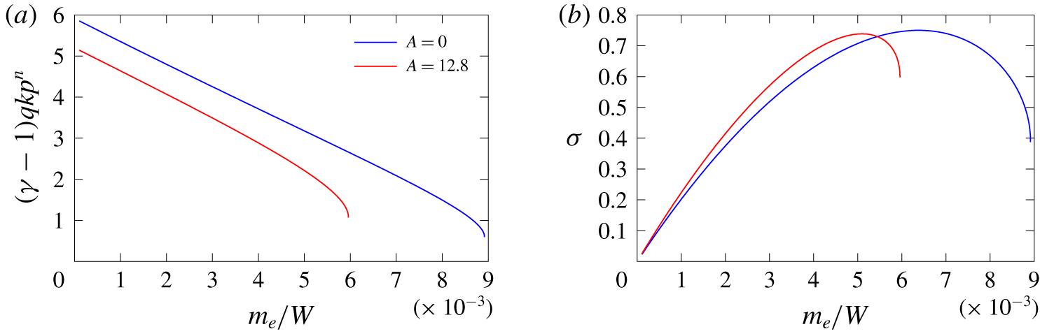
Figure 5. Sonic flow point variation of (a) $(\unicode[STIX]{x1D6FE}-1)qkp^{n}$
and (b)
$(\unicode[STIX]{x1D6FE}-1)qkp^{n}$
and (b) $\unicode[STIX]{x1D70E}$
, the energy change associated with the rate of change of mass flux through the detonation due to the boundary streamline deflection, as a function of
$\unicode[STIX]{x1D70E}$
, the energy change associated with the rate of change of mass flux through the detonation due to the boundary streamline deflection, as a function of $m_{e}/W$
for
$m_{e}/W$
for $A=0$
and
$A=0$
and $A=12.8$
for
$A=12.8$
for $s=0,n=2$
and
$s=0,n=2$
and $\unicode[STIX]{x1D708}=0.5$
.
$\unicode[STIX]{x1D708}=0.5$
.
Figure 5(a,b) shows the variation of the reaction rate related energy factor $(\unicode[STIX]{x1D6FE}-1)qkp^{n}$
and
$(\unicode[STIX]{x1D6FE}-1)qkp^{n}$
and $\unicode[STIX]{x1D70E}$
with
$\unicode[STIX]{x1D70E}$
with $m_{e}/W$
at the sonic flow point for
$m_{e}/W$
at the sonic flow point for $s=0,n=2$
and
$s=0,n=2$
and $\unicode[STIX]{x1D708}=0.5$
and for
$\unicode[STIX]{x1D708}=0.5$
and for $A=0$
and
$A=0$
and $A=12.8.$
The behaviour for
$A=12.8.$
The behaviour for $A=6.4$
lies between that of
$A=6.4$
lies between that of $A=0$
and
$A=0$
and $A=12.8$
. Interestingly, in both cases, the
$A=12.8$
. Interestingly, in both cases, the $\unicode[STIX]{x1D70E}$
variation is non-monotonic, first increasing as
$\unicode[STIX]{x1D70E}$
variation is non-monotonic, first increasing as $m_{e}/W$
increases, before decreasing near the failure point. The ratio
$m_{e}/W$
increases, before decreasing near the failure point. The ratio $\unicode[STIX]{x1D70E}/(\unicode[STIX]{x1D6FE}-1)qkp^{n}$
is
$\unicode[STIX]{x1D70E}/(\unicode[STIX]{x1D6FE}-1)qkp^{n}$
is $(1-\unicode[STIX]{x1D706})^{\unicode[STIX]{x1D708}}$
. For both
$(1-\unicode[STIX]{x1D706})^{\unicode[STIX]{x1D708}}$
. For both $A=0$
and
$A=0$
and $A=12.8,\unicode[STIX]{x1D70E}<(\unicode[STIX]{x1D6FE}-1)qkp^{n}$
for all
$A=12.8,\unicode[STIX]{x1D70E}<(\unicode[STIX]{x1D6FE}-1)qkp^{n}$
for all $m_{e}/W$
with the ratio
$m_{e}/W$
with the ratio $\unicode[STIX]{x1D70E}/(\unicode[STIX]{x1D6FE}-1)qkp^{n}$
increasing monotonically from zero as
$\unicode[STIX]{x1D70E}/(\unicode[STIX]{x1D6FE}-1)qkp^{n}$
increasing monotonically from zero as $m_{e}/W$
increases. Consequently, the value of
$m_{e}/W$
increases. Consequently, the value of $\unicode[STIX]{x1D706}$
at the sonic point,
$\unicode[STIX]{x1D706}$
at the sonic point, $\unicode[STIX]{x1D706}_{s},$
must decrease with increasing
$\unicode[STIX]{x1D706}_{s},$
must decrease with increasing $m_{e}/W$
(figure 4
b) to ensure that the chemical energy term
$m_{e}/W$
(figure 4
b) to ensure that the chemical energy term $(\unicode[STIX]{x1D6FE}-1)q\unicode[STIX]{x1D6EC}$
and the energy term
$(\unicode[STIX]{x1D6FE}-1)q\unicode[STIX]{x1D6EC}$
and the energy term $\unicode[STIX]{x1D70E}$
, associated with the rate of change of mass flux, cancel at the sonic point.
$\unicode[STIX]{x1D70E}$
, associated with the rate of change of mass flux, cancel at the sonic point.
Further insights into the $D_{0}$
versus
$D_{0}$
versus $m_{e}/W$
behaviour seen in figure 4(a) can be obtained from figure 6(a) which shows a comparison for
$m_{e}/W$
behaviour seen in figure 4(a) can be obtained from figure 6(a) which shows a comparison for $A=0$
and
$A=0$
and $A=12.8$
of the variation of
$A=12.8$
of the variation of $(\unicode[STIX]{x1D6FE}-1)q\unicode[STIX]{x1D6EC}$
,
$(\unicode[STIX]{x1D6FE}-1)q\unicode[STIX]{x1D6EC}$
, $\unicode[STIX]{x1D70E}$
and
$\unicode[STIX]{x1D70E}$
and $\unicode[STIX]{x1D714}$
with
$\unicode[STIX]{x1D714}$
with $\unicode[STIX]{x1D702}$
for
$\unicode[STIX]{x1D702}$
for $m_{e}/W=0.005,s=0,n=2$
and
$m_{e}/W=0.005,s=0,n=2$
and $\unicode[STIX]{x1D708}=0.5$
. For
$\unicode[STIX]{x1D708}=0.5$
. For $A=0$
,
$A=0$
, $D_{0}=6.945$
at
$D_{0}=6.945$
at $m_{e}/W=0.005,$
while for
$m_{e}/W=0.005,$
while for $A=12.8,D_{0}=6.732.$
Near the shock
$A=12.8,D_{0}=6.732.$
Near the shock $(\unicode[STIX]{x1D702}=0),$
the energy term
$(\unicode[STIX]{x1D702}=0),$
the energy term $(\unicode[STIX]{x1D6FE}-1)q\unicode[STIX]{x1D6EC}$
associated with chemical reaction is significantly greater for
$(\unicode[STIX]{x1D6FE}-1)q\unicode[STIX]{x1D6EC}$
associated with chemical reaction is significantly greater for $A=0$
than
$A=0$
than $A=12.8$
as also seen for the ZND wave structure (§ 5), with the variations for
$A=12.8$
as also seen for the ZND wave structure (§ 5), with the variations for $A=0$
and
$A=0$
and $A=12.8$
decreasing monotonically with increasing
$A=12.8$
decreasing monotonically with increasing $|\unicode[STIX]{x1D702}|,$
until the sonic flow point
$|\unicode[STIX]{x1D702}|,$
until the sonic flow point $\unicode[STIX]{x1D714}=0$
is reached. Similarly, the sonic parameter
$\unicode[STIX]{x1D714}=0$
is reached. Similarly, the sonic parameter $\unicode[STIX]{x1D714}$
is uniformly larger for
$\unicode[STIX]{x1D714}$
is uniformly larger for $A=0$
than
$A=0$
than $A=12.8,$
with again both variations decreasing monotonically. The energy term
$A=12.8,$
with again both variations decreasing monotonically. The energy term $\unicode[STIX]{x1D70E}$
shows less of a difference between
$\unicode[STIX]{x1D70E}$
shows less of a difference between $A=0$
and
$A=0$
and $A=12.8.$
At the sonic flow points,
$A=12.8.$
At the sonic flow points, $(\unicode[STIX]{x1D6FE}-1)q\unicode[STIX]{x1D6EC}-\unicode[STIX]{x1D70E}=0$
with
$(\unicode[STIX]{x1D6FE}-1)q\unicode[STIX]{x1D6EC}-\unicode[STIX]{x1D70E}=0$
with $\unicode[STIX]{x1D714}=0.$
Figure 6(b) shows the corresponding variation of
$\unicode[STIX]{x1D714}=0.$
Figure 6(b) shows the corresponding variation of $(c^{0})^{2}\unicode[STIX]{x1D70C}_{0}D_{0}/\unicode[STIX]{x1D70C}^{0}$
and
$(c^{0})^{2}\unicode[STIX]{x1D70C}_{0}D_{0}/\unicode[STIX]{x1D70C}^{0}$
and $(\unicode[STIX]{x1D6FE}-1)qkp^{n}$
with
$(\unicode[STIX]{x1D6FE}-1)qkp^{n}$
with $\unicode[STIX]{x1D702}$
for
$\unicode[STIX]{x1D702}$
for $m_{e}/W=0.005.$
The term
$m_{e}/W=0.005.$
The term $(c^{0})^{2}\unicode[STIX]{x1D70C}_{0}D_{0}/\unicode[STIX]{x1D70C}^{0}$
is the coefficient multiplying the boundary streamline deflection influence in
$(c^{0})^{2}\unicode[STIX]{x1D70C}_{0}D_{0}/\unicode[STIX]{x1D70C}^{0}$
is the coefficient multiplying the boundary streamline deflection influence in $\unicode[STIX]{x1D70E}$
for
$\unicode[STIX]{x1D70E}$
for $s=0$
(see (5.7)), with
$s=0$
(see (5.7)), with $h(\unicode[STIX]{x1D702})=\unicode[STIX]{x1D702}.$
Thus, for fixed
$h(\unicode[STIX]{x1D702})=\unicode[STIX]{x1D702}.$
Thus, for fixed $m_{e}/W$
, the variation in
$m_{e}/W$
, the variation in $\unicode[STIX]{x1D70E}$
enters through this coefficient term. The term
$\unicode[STIX]{x1D70E}$
enters through this coefficient term. The term $(\unicode[STIX]{x1D6FE}-1)qkp^{n}$
is the coefficient term multiplying
$(\unicode[STIX]{x1D6FE}-1)qkp^{n}$
is the coefficient term multiplying $(1-\unicode[STIX]{x1D706})^{\unicode[STIX]{x1D708}}$
in the energy term
$(1-\unicode[STIX]{x1D706})^{\unicode[STIX]{x1D708}}$
in the energy term $(\unicode[STIX]{x1D6FE}-1)q\unicode[STIX]{x1D6EC}$
. Thus, at the sonic point, we must have
$(\unicode[STIX]{x1D6FE}-1)q\unicode[STIX]{x1D6EC}$
. Thus, at the sonic point, we must have
 $$\begin{eqnarray}\frac{[(1-\unicode[STIX]{x1D706})^{\unicode[STIX]{x1D708}}]_{A=12.8}}{[(1-\unicode[STIX]{x1D706})^{\unicode[STIX]{x1D708}}]_{A=0}}=\frac{[(c^{0})^{2}\unicode[STIX]{x1D70C}_{0}D_{0}/\unicode[STIX]{x1D70C}^{0}]_{A=12.8}[(\unicode[STIX]{x1D6FE}-1)qkp^{n}]_{A=0}}{[(c^{0})^{2}\unicode[STIX]{x1D70C}_{0}D_{0}/\unicode[STIX]{x1D70C}^{0}]_{A=0}[(\unicode[STIX]{x1D6FE}-1)qkp^{n}]_{A=12.8}}.\end{eqnarray}$$
Now, $[(c^{0})^{2}\unicode[STIX]{x1D70C}_{0}D_{0}/\unicode[STIX]{x1D70C}^{0}]_{A=12.8}>[(c^{0})^{2}\unicode[STIX]{x1D70C}_{0}D_{0}/\unicode[STIX]{x1D70C}^{0}]_{A=0}$
(figure 6
b) but with the ratio close to one. However, with
$[(c^{0})^{2}\unicode[STIX]{x1D70C}_{0}D_{0}/\unicode[STIX]{x1D70C}^{0}]_{A=12.8}>[(c^{0})^{2}\unicode[STIX]{x1D70C}_{0}D_{0}/\unicode[STIX]{x1D70C}^{0}]_{A=0}$
(figure 6
b) but with the ratio close to one. However, with $[(\unicode[STIX]{x1D6FE}-1)qkp^{n}]_{A=0}>[(\unicode[STIX]{x1D6FE}-1)qkp^{n}]_{A=12.8}$
, a result of the equation-of-state dependence on
$[(\unicode[STIX]{x1D6FE}-1)qkp^{n}]_{A=0}>[(\unicode[STIX]{x1D6FE}-1)qkp^{n}]_{A=12.8}$
, a result of the equation-of-state dependence on $A$
manifested through the decrease in pressure for increasing
$A$
manifested through the decrease in pressure for increasing $A,$
then
$A,$
then $[(1-\unicode[STIX]{x1D706})^{\unicode[STIX]{x1D708}}]_{A=12.8}>[(1-\unicode[STIX]{x1D706})^{\unicode[STIX]{x1D708}}]_{A=0}$
. Consequently,
$[(1-\unicode[STIX]{x1D706})^{\unicode[STIX]{x1D708}}]_{A=12.8}>[(1-\unicode[STIX]{x1D706})^{\unicode[STIX]{x1D708}}]_{A=0}$
. Consequently, $\unicode[STIX]{x1D706}$
at the sonic point,
$\unicode[STIX]{x1D706}$
at the sonic point, $\unicode[STIX]{x1D706}_{s},$
for
$\unicode[STIX]{x1D706}_{s},$
for $A=12.8$
must be smaller than
$A=12.8$
must be smaller than $\unicode[STIX]{x1D706}_{s}$
for
$\unicode[STIX]{x1D706}_{s}$
for $A=0$
, since
$A=0$
, since $\unicode[STIX]{x1D708}$
is fixed, as shown in figure 4(b). The DDZ is thus terminated when
$\unicode[STIX]{x1D708}$
is fixed, as shown in figure 4(b). The DDZ is thus terminated when $\unicode[STIX]{x1D714}=0$
at a point of more incomplete reaction as
$\unicode[STIX]{x1D714}=0$
at a point of more incomplete reaction as $A$
is increased.
$A$
is increased.

Figure 6. Variation of (a) $(\unicode[STIX]{x1D6FE}-1)q\unicode[STIX]{x1D6EC}$
,
$(\unicode[STIX]{x1D6FE}-1)q\unicode[STIX]{x1D6EC}$
, $\unicode[STIX]{x1D70E}$
and
$\unicode[STIX]{x1D70E}$
and $\unicode[STIX]{x1D714}$
for
$\unicode[STIX]{x1D714}$
for $A=0$
(dashed lines) and
$A=0$
(dashed lines) and $A=12.8$
(solid lines) and (b)
$A=12.8$
(solid lines) and (b) $(c^{0})^{2}\unicode[STIX]{x1D70C}_{0}D_{0}/\unicode[STIX]{x1D70C}^{0}$
(solid lines) and
$(c^{0})^{2}\unicode[STIX]{x1D70C}_{0}D_{0}/\unicode[STIX]{x1D70C}^{0}$
(solid lines) and $(\unicode[STIX]{x1D6FE}-1)qkp^{n}$
(dashed lines) for
$(\unicode[STIX]{x1D6FE}-1)qkp^{n}$
(dashed lines) for $A=0$
and
$A=0$
and $A=12.8$
as a function of
$A=12.8$
as a function of $\unicode[STIX]{x1D702}$
for
$\unicode[STIX]{x1D702}$
for $m_{e}/W=0.005,s=0,n=2$
and
$m_{e}/W=0.005,s=0,n=2$
and $\unicode[STIX]{x1D708}=0.5$
.
$\unicode[STIX]{x1D708}=0.5$
.

Figure 7. A rescaling of figure 4(a), showing the variation of $D_{0}$
now with
$D_{0}$
now with $(1+s)m_{e}/W_{\unicode[STIX]{x1D702}_{s}}$
for slab (
$(1+s)m_{e}/W_{\unicode[STIX]{x1D702}_{s}}$
for slab ( $s=0$
) and cylindrical (
$s=0$
) and cylindrical ( $s=1$
) geometries with
$s=1$
) geometries with $n=2$
and
$n=2$
and $\unicode[STIX]{x1D708}=0.5$
and for
$\unicode[STIX]{x1D708}=0.5$
and for $A=0$
,
$A=0$
, $A=6.4$
and
$A=6.4$
and $A=12.8$
.
$A=12.8$
.
We have previously noted in figure 4(b) the increase in $|\unicode[STIX]{x1D702}_{s}|$
as
$|\unicode[STIX]{x1D702}_{s}|$
as $m_{e}/W$
increases, with the fixed reference length scale
$m_{e}/W$
increases, with the fixed reference length scale $\tilde{l}_{1/2}$
adopted (§ 5). As discussed in § 5, the alternative length scale
$\tilde{l}_{1/2}$
adopted (§ 5). As discussed in § 5, the alternative length scale $\tilde{l}_{\unicode[STIX]{x1D702}_{s}}$
, as guided by the asymptotic analysis (§ 4), represents the distance between the detonation shock and sonic flow point. Adopting the reference length scale
$\tilde{l}_{\unicode[STIX]{x1D702}_{s}}$
, as guided by the asymptotic analysis (§ 4), represents the distance between the detonation shock and sonic flow point. Adopting the reference length scale $\tilde{l}_{\unicode[STIX]{x1D702}_{s}}$
rescales
$\tilde{l}_{\unicode[STIX]{x1D702}_{s}}$
rescales $\unicode[STIX]{x1D702}_{s}=-1$
in all cases, and allows us to recast figure 4(a) in terms of
$\unicode[STIX]{x1D702}_{s}=-1$
in all cases, and allows us to recast figure 4(a) in terms of $W_{\unicode[STIX]{x1D702}_{s}}$
. The rescaling of figure 4(a) is presented in figure 7. Although the asymptotic results are identical, just that
$W_{\unicode[STIX]{x1D702}_{s}}$
. The rescaling of figure 4(a) is presented in figure 7. Although the asymptotic results are identical, just that $W$
has been rescaled to
$W$
has been rescaled to $W_{\unicode[STIX]{x1D702}_{s}}$
based on setting
$W_{\unicode[STIX]{x1D702}_{s}}$
based on setting $\unicode[STIX]{x1D702}_{s}=-1$
, we observe an increase in numerical size of
$\unicode[STIX]{x1D702}_{s}=-1$
, we observe an increase in numerical size of $m_{e}/W_{\unicode[STIX]{x1D702}_{s}}$
relative to
$m_{e}/W_{\unicode[STIX]{x1D702}_{s}}$
relative to $m_{e}/W$
, verifying the description of the role of the length scale choice discussed in § 5. However, with
$m_{e}/W$
, verifying the description of the role of the length scale choice discussed in § 5. However, with $\tilde{l}_{\unicode[STIX]{x1D702}_{s}}$
, as each separate confinement case for varying
$\tilde{l}_{\unicode[STIX]{x1D702}_{s}}$
, as each separate confinement case for varying $m_{e}$
and channel width will have a different reference length scale, we proceed with using the fixed scale
$m_{e}$
and channel width will have a different reference length scale, we proceed with using the fixed scale $\tilde{l}_{1/2}$
as the chosen reference scale for clarity of discussion.
$\tilde{l}_{1/2}$
as the chosen reference scale for clarity of discussion.
We now explore the effect of varying the pressure exponent $n$
in the reaction rate (5.3) for fixed
$n$
in the reaction rate (5.3) for fixed $A$
and
$A$
and $\unicode[STIX]{x1D708}.$
Figure 8(a) shows the variation of the asymptotically derived propagation speed
$\unicode[STIX]{x1D708}.$
Figure 8(a) shows the variation of the asymptotically derived propagation speed $D_{0}$
from (5.7) with
$D_{0}$
from (5.7) with $m_{e}/W$
for
$m_{e}/W$
for $A=12.8,s=0,\unicode[STIX]{x1D708}=1/2$
and
$A=12.8,s=0,\unicode[STIX]{x1D708}=1/2$
and $n=1.75,n=2$
and
$n=1.75,n=2$
and $n=2.25.$
Again, each curve is characterized by a monotonic decrease in
$n=2.25.$
Again, each curve is characterized by a monotonic decrease in $D_{0}$
with increasing
$D_{0}$
with increasing $m_{e}/W$
and a critical value of
$m_{e}/W$
and a critical value of $m_{e}/W,$
beyond which no steady solutions are possible, corresponding to a turning point in the
$m_{e}/W,$
beyond which no steady solutions are possible, corresponding to a turning point in the $D_{0}$
versus
$D_{0}$
versus $m_{e}/W$
relation. The speed
$m_{e}/W$
relation. The speed $D_{0}$
decreases more rapidly with
$D_{0}$
decreases more rapidly with $m_{e}/W$
as
$m_{e}/W$
as $n$
increases, with the critical value of
$n$
increases, with the critical value of $m_{e}/W$
also decreasing as
$m_{e}/W$
also decreasing as $n$
increases, while
$n$
increases, while $D_{0}$
increases at the critical point. Consequently, for a fixed charge width
$D_{0}$
increases at the critical point. Consequently, for a fixed charge width $W,$
the larger the rate exponent
$W,$
the larger the rate exponent $n$
the smaller the boundary streamline deflection the detonation can withstand. This implies that a detonation in an HE with a lower reaction rate state-sensitivity (smaller
$n$
the smaller the boundary streamline deflection the detonation can withstand. This implies that a detonation in an HE with a lower reaction rate state-sensitivity (smaller $n$
) is more capable of propagating when confined by materials with smaller impedances over one with a larger state sensitivity (larger
$n$
) is more capable of propagating when confined by materials with smaller impedances over one with a larger state sensitivity (larger $n$
). Note that increases in
$n$
). Note that increases in $n$
are associated with a longer reaction tail in the ZND structure (§ 5). Here, we conjecture that as the reaction rate is weakened in the tail, a given boundary streamline deflection gradient will lead to more of the reaction being cutoff in the DDZ to achieve the reaction rate required to balance the energy loss term
$n$
are associated with a longer reaction tail in the ZND structure (§ 5). Here, we conjecture that as the reaction rate is weakened in the tail, a given boundary streamline deflection gradient will lead to more of the reaction being cutoff in the DDZ to achieve the reaction rate required to balance the energy loss term $\unicode[STIX]{x1D70E}.$
This is indeed the case, as shown in figure 8(b). For each
$\unicode[STIX]{x1D70E}.$
This is indeed the case, as shown in figure 8(b). For each $n,$
as
$n,$
as $m_{e}/W$
increases, the reaction progress variable at the sonic point decreases as
$m_{e}/W$
increases, the reaction progress variable at the sonic point decreases as $m_{e}/W$
increases, while the sonic flow location moves increasingly downstream of the shock, i.e. the DDZ length increases. Moreover, at any fixed
$m_{e}/W$
increases, while the sonic flow location moves increasingly downstream of the shock, i.e. the DDZ length increases. Moreover, at any fixed $m_{e}/W$
, the reaction progress variable at the sonic point is smaller as
$m_{e}/W$
, the reaction progress variable at the sonic point is smaller as $n$
increases. The variation of
$n$
increases. The variation of $(c^{0})^{2}\unicode[STIX]{x1D70C}_{0}D_{0}/\unicode[STIX]{x1D70C}^{0}$
and
$(c^{0})^{2}\unicode[STIX]{x1D70C}_{0}D_{0}/\unicode[STIX]{x1D70C}^{0}$
and $(\unicode[STIX]{x1D6FE}-1)qkp^{n}$
with
$(\unicode[STIX]{x1D6FE}-1)qkp^{n}$
with $\unicode[STIX]{x1D702}$
for
$\unicode[STIX]{x1D702}$
for $m_{e}/W=0.004,s=0,\unicode[STIX]{x1D708}=1/2$
and
$m_{e}/W=0.004,s=0,\unicode[STIX]{x1D708}=1/2$
and $n=1.75$
(
$n=1.75$
( $D_{0}=7.251$
) and
$D_{0}=7.251$
) and $n=2.25$
(
$n=2.25$
( $D_{0}=6.814$
) are shown in figure 9(a) . At the sonic point,
$D_{0}=6.814$
) are shown in figure 9(a) . At the sonic point,
 $$\begin{eqnarray}\frac{[(1-\unicode[STIX]{x1D706})^{\unicode[STIX]{x1D708}}]_{n=1.75}}{[(1-\unicode[STIX]{x1D706})^{\unicode[STIX]{x1D708}}]_{n=2.25}}=\frac{[(c^{0})^{2}\unicode[STIX]{x1D70C}_{0}D_{0}/\unicode[STIX]{x1D70C}^{0}]_{n=1.75}}{[(c^{0})^{2}\unicode[STIX]{x1D70C}_{0}D_{0}/\unicode[STIX]{x1D70C}^{0}]_{n=2.25}}\frac{[(\unicode[STIX]{x1D6FE}-1)qkp^{n}]_{n=2.25}}{[(\unicode[STIX]{x1D6FE}-1)qkp^{n}]_{n=1.75}}.\end{eqnarray}$$
From figure 9(a), the right-hand side is dominated by the factor
 $$\begin{eqnarray}[(\unicode[STIX]{x1D6FE}-1)qkp^{n}]_{n=2.25}/[(\unicode[STIX]{x1D6FE}-1)qkp^{n}]_{n=1.75},\end{eqnarray}$$
where $[(\unicode[STIX]{x1D6FE}-1)qkp^{n}]_{n=2.25}\ll [(\unicode[STIX]{x1D6FE}-1)qkp^{n}]_{n=1.75}$
, so that
$[(\unicode[STIX]{x1D6FE}-1)qkp^{n}]_{n=2.25}\ll [(\unicode[STIX]{x1D6FE}-1)qkp^{n}]_{n=1.75}$
, so that $[(1-\unicode[STIX]{x1D706})^{\unicode[STIX]{x1D708}}]_{n=1.75}<[(1-\unicode[STIX]{x1D706})^{\unicode[STIX]{x1D708}}]_{n=2.25}$
and
$[(1-\unicode[STIX]{x1D706})^{\unicode[STIX]{x1D708}}]_{n=1.75}<[(1-\unicode[STIX]{x1D706})^{\unicode[STIX]{x1D708}}]_{n=2.25}$
and $[\unicode[STIX]{x1D706}_{s}]_{n=2.25}<[\unicode[STIX]{x1D706}_{s}]_{n=1.75}.$
Thus, the decrease in reaction rate in the reaction tail as
$[\unicode[STIX]{x1D706}_{s}]_{n=2.25}<[\unicode[STIX]{x1D706}_{s}]_{n=1.75}.$
Thus, the decrease in reaction rate in the reaction tail as $n$
increases results in the DDZ terminating at a point of more incomplete reaction, as conjectured.
$n$
increases results in the DDZ terminating at a point of more incomplete reaction, as conjectured.

Figure 8. (a) Variation of $D_{0}$
with
$D_{0}$
with $m_{e}/W$
for
$m_{e}/W$
for $s=0$
,
$s=0$
, $A=12.8$
,
$A=12.8$
, $\unicode[STIX]{x1D708}=0.5$
and
$\unicode[STIX]{x1D708}=0.5$
and $n=1.75$
(
$n=1.75$
( $k=2.61113\times 10^{-3}$
),
$k=2.61113\times 10^{-3}$
), $n=2$
(
$n=2$
( $k=9.67560\times 10^{-4}$
) and
$k=9.67560\times 10^{-4}$
) and $n=2.25$
(
$n=2.25$
( $k=3.58579\times 10^{-4}$
). (b) The corresponding variation in
$k=3.58579\times 10^{-4}$
). (b) The corresponding variation in $\unicode[STIX]{x1D702}_{s}$
(solid lines) and
$\unicode[STIX]{x1D702}_{s}$
(solid lines) and $\unicode[STIX]{x1D706}_{s}$
(dashed lines).
$\unicode[STIX]{x1D706}_{s}$
(dashed lines).
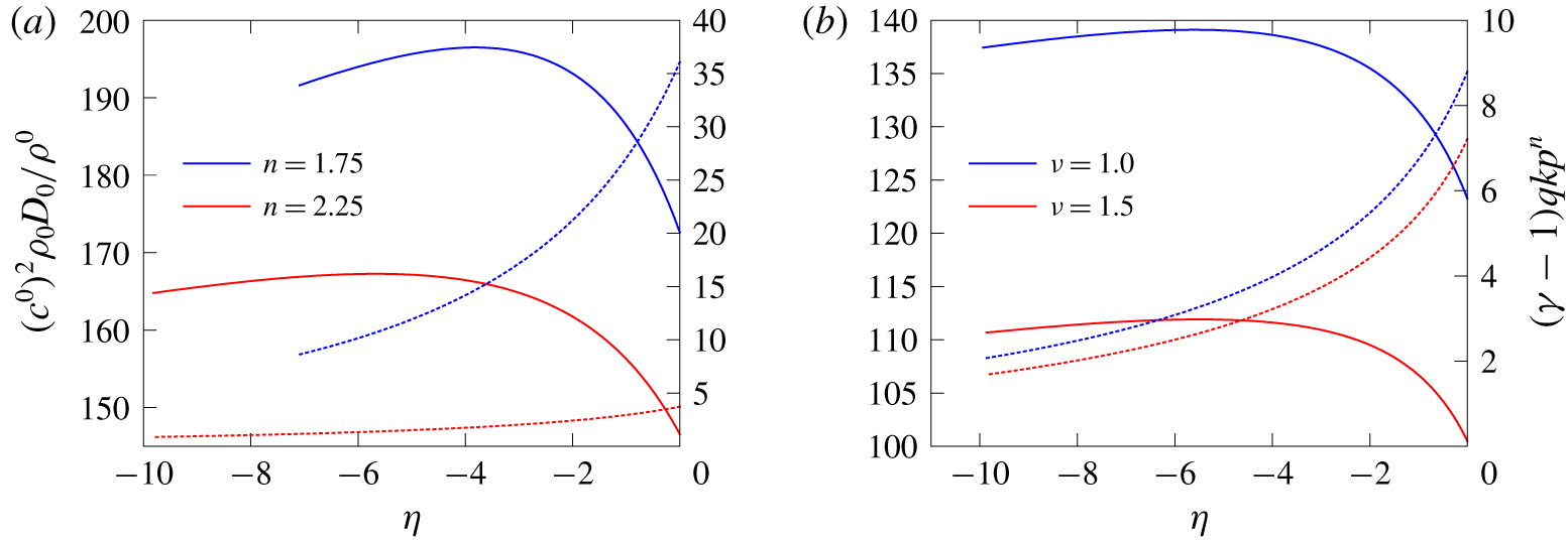
Figure 9. Variation of $(c^{0})^{2}\unicode[STIX]{x1D70C}_{0}D_{0}/\unicode[STIX]{x1D70C}^{0}$
(solid lines) and
$(c^{0})^{2}\unicode[STIX]{x1D70C}_{0}D_{0}/\unicode[STIX]{x1D70C}^{0}$
(solid lines) and $(\unicode[STIX]{x1D6FE}-1)qkp^{n}$
(dashed lines) as a function of
$(\unicode[STIX]{x1D6FE}-1)qkp^{n}$
(dashed lines) as a function of $\unicode[STIX]{x1D702}$
for
$\unicode[STIX]{x1D702}$
for $A=12.8,m_{e}/W=0.004,s=0,$
and (a)
$A=12.8,m_{e}/W=0.004,s=0,$
and (a) $\unicode[STIX]{x1D708}=0.5,n=1.75$
and
$\unicode[STIX]{x1D708}=0.5,n=1.75$
and $n=2.25$
and (b)
$n=2.25$
and (b) $n=2,\unicode[STIX]{x1D708}=1$
and
$n=2,\unicode[STIX]{x1D708}=1$
and $\unicode[STIX]{x1D708}=1.5.$

Figure 10. (a) Variation of $D_{0}$
with
$D_{0}$
with $m_{e}/W$
for
$m_{e}/W$
for $s=0$
,
$s=0$
, $A=12.8$
,
$A=12.8$
, $n=2$
and
$n=2$
and $\unicode[STIX]{x1D708}=0.5$
(
$\unicode[STIX]{x1D708}=0.5$
( $k=9.67560\times 10^{-4}$
),
$k=9.67560\times 10^{-4}$
), $\unicode[STIX]{x1D708}=1$
(
$\unicode[STIX]{x1D708}=1$
( $k=1.15912\times 10^{-3}$
) and
$k=1.15912\times 10^{-3}$
) and $\unicode[STIX]{x1D708}=1.5$
(
$\unicode[STIX]{x1D708}=1.5$
( $k=1.40239\times 10^{-3}$
). (b) The corresponding variation in
$k=1.40239\times 10^{-3}$
). (b) The corresponding variation in $\unicode[STIX]{x1D702}_{s}$
(solid lines) and
$\unicode[STIX]{x1D702}_{s}$
(solid lines) and $\unicode[STIX]{x1D706}_{s}$
(dashed lines).
$\unicode[STIX]{x1D706}_{s}$
(dashed lines).
Finally, we explore the effect of varying the reaction order in the rate form (5.3) for fixed $A$
and
$A$
and $n.$
Figure 10(a) shows the variation of the asymptotically derived solution for
$n.$
Figure 10(a) shows the variation of the asymptotically derived solution for $D_{0}$
from (5.7) with
$D_{0}$
from (5.7) with $m_{e}/W$
for
$m_{e}/W$
for $A=12.8,s=0,n=2$
and
$A=12.8,s=0,n=2$
and $\unicode[STIX]{x1D708}=0.5,\unicode[STIX]{x1D708}=1$
and
$\unicode[STIX]{x1D708}=0.5,\unicode[STIX]{x1D708}=1$
and $\unicode[STIX]{x1D708}=1.5.$
Figure 10(b) shows the variation in the location of the sonic point relative to the shock
$\unicode[STIX]{x1D708}=1.5.$
Figure 10(b) shows the variation in the location of the sonic point relative to the shock $(\unicode[STIX]{x1D702}=0)$
and the value of the reactant progress variable
$(\unicode[STIX]{x1D702}=0)$
and the value of the reactant progress variable $\unicode[STIX]{x1D706}_{s}$
at the sonic flow point as a function of
$\unicode[STIX]{x1D706}_{s}$
at the sonic flow point as a function of $m_{e}/W.$
Increasing the reaction order leads to a more rapid drop in
$m_{e}/W.$
Increasing the reaction order leads to a more rapid drop in $D_{0}$
as
$D_{0}$
as $m_{e}/W$
increases (figure 10
a). The value of
$m_{e}/W$
increases (figure 10
a). The value of $m_{e}/W$
at the critical point is reduced for increasing
$m_{e}/W$
at the critical point is reduced for increasing $\unicode[STIX]{x1D708},$
while
$\unicode[STIX]{x1D708},$
while $D_{0}$
also decreases at the critical point for increasing
$D_{0}$
also decreases at the critical point for increasing $\unicode[STIX]{x1D708}.$
The latter feature differs from the
$\unicode[STIX]{x1D708}.$
The latter feature differs from the $D_{0}$
behaviour at the critical point for increasing
$D_{0}$
behaviour at the critical point for increasing $A$
and
$A$
and $n$
. Increasing the reaction order leads to a higher reaction rate at the shock, but a longer reaction tail (§ 5). The length of the ZND wave is formally infinite for
$n$
. Increasing the reaction order leads to a higher reaction rate at the shock, but a longer reaction tail (§ 5). The length of the ZND wave is formally infinite for $\unicode[STIX]{x1D708}\geqslant 1$
, while the DDZ length for
$\unicode[STIX]{x1D708}\geqslant 1$
, while the DDZ length for $m_{e}/W>0$
is finite and shortens as
$m_{e}/W>0$
is finite and shortens as $m_{e}/W$
increases. For
$m_{e}/W$
increases. For $\unicode[STIX]{x1D708}=1,$
the DDZ length reaches a minimum near the critical point before increasing again. The reaction progress variable at the sonic point decreases for each
$\unicode[STIX]{x1D708}=1,$
the DDZ length reaches a minimum near the critical point before increasing again. The reaction progress variable at the sonic point decreases for each $\unicode[STIX]{x1D708}$
as
$\unicode[STIX]{x1D708}$
as $m_{e}/W$
increases, with a more rapid decrease as
$m_{e}/W$
increases, with a more rapid decrease as $\unicode[STIX]{x1D708}$
increases (figure 10
b). Figure 9(b) shows the variation of
$\unicode[STIX]{x1D708}$
increases (figure 10
b). Figure 9(b) shows the variation of $(c^{0})^{2}\unicode[STIX]{x1D70C}_{0}D_{0}/\unicode[STIX]{x1D70C}^{0}$
and
$(c^{0})^{2}\unicode[STIX]{x1D70C}_{0}D_{0}/\unicode[STIX]{x1D70C}^{0}$
and $(\unicode[STIX]{x1D6FE}-1)qkp^{n}$
with
$(\unicode[STIX]{x1D6FE}-1)qkp^{n}$
with $\unicode[STIX]{x1D702}$
for
$\unicode[STIX]{x1D702}$
for $m_{e}/W=0.004,s=0,n=2$
and
$m_{e}/W=0.004,s=0,n=2$
and $\unicode[STIX]{x1D708}=1$
(
$\unicode[STIX]{x1D708}=1$
( $D_{0}=6.373$
) and
$D_{0}=6.373$
) and $\unicode[STIX]{x1D708}=1.5$
(
$\unicode[STIX]{x1D708}=1.5$
( $D_{0}=5.880$
). As before, at the sonic point,
$D_{0}=5.880$
). As before, at the sonic point,
 $$\begin{eqnarray}\frac{[(1-\unicode[STIX]{x1D706})^{\unicode[STIX]{x1D708}}]_{\unicode[STIX]{x1D708}=1}}{[(1-\unicode[STIX]{x1D706})^{\unicode[STIX]{x1D708}}]_{\unicode[STIX]{x1D708}=1.5}}=\frac{[(c^{0})^{2}\unicode[STIX]{x1D70C}_{0}D_{0}/\unicode[STIX]{x1D70C}^{0}]_{\unicode[STIX]{x1D708}=1}}{[(c^{0})^{2}\unicode[STIX]{x1D70C}_{0}D_{0}/\unicode[STIX]{x1D70C}^{0}]_{\unicode[STIX]{x1D708}=1.5}}\frac{[(\unicode[STIX]{x1D6FE}-1)qkp^{n}]_{\unicode[STIX]{x1D708}=1.5}}{[(\unicode[STIX]{x1D6FE}-1)qkp^{n}]_{\unicode[STIX]{x1D708}=1}}.\end{eqnarray}$$
Unlike the previous cases, from figure 9(b), the ratio on the right-hand side is approximately one (≈1. 016), and thus the observed variation in $\unicode[STIX]{x1D706}_{s}$
(figure 10
b) is a result of the reaction-order dependence of the rate term. With the right-hand side of (6.3) being close to one, we must have
$\unicode[STIX]{x1D706}_{s}$
(figure 10
b) is a result of the reaction-order dependence of the rate term. With the right-hand side of (6.3) being close to one, we must have $[\unicode[STIX]{x1D706}_{s}]_{\unicode[STIX]{x1D708}=1}>[\unicode[STIX]{x1D706}_{s}]_{\unicode[STIX]{x1D708}=1.5},$
confirming the results seen in figure 10(b). In summary, increasing the stiffened constant
$[\unicode[STIX]{x1D706}_{s}]_{\unicode[STIX]{x1D708}=1}>[\unicode[STIX]{x1D706}_{s}]_{\unicode[STIX]{x1D708}=1.5},$
confirming the results seen in figure 10(b). In summary, increasing the stiffened constant $A,$
pressure rate exponent
$A,$
pressure rate exponent $n$
and reaction order
$n$
and reaction order $\unicode[STIX]{x1D708}$
causes
$\unicode[STIX]{x1D708}$
causes $D_{0}$
to drop more rapidly as
$D_{0}$
to drop more rapidly as $m_{e}/W$
increases, leading to smaller values of
$m_{e}/W$
increases, leading to smaller values of $m_{e}/W$
at which the critical point is reached, i.e. in each case, the detonation’s ability to overcome the energy deficit caused by the rate of change of mass flux through the wave associated with the boundary streamline deflection is diminished.
$m_{e}/W$
at which the critical point is reached, i.e. in each case, the detonation’s ability to overcome the energy deficit caused by the rate of change of mass flux through the wave associated with the boundary streamline deflection is diminished.
In order to ascertain the accuracy of the asymptotic analysis in § 4, we now compare the asymptotically calculated variation of $D_{0}$
obtained from (5.7) with varying boundary streamline deflection angle
$D_{0}$
obtained from (5.7) with varying boundary streamline deflection angle $\unicode[STIX]{x1D703}_{e}$
(where
$\unicode[STIX]{x1D703}_{e}$
(where $m_{e}=\tan \unicode[STIX]{x1D703}_{e},$
§ 2) for
$m_{e}=\tan \unicode[STIX]{x1D703}_{e},$
§ 2) for $A=0,n=2,\unicode[STIX]{x1D708}=0.5$
and
$A=0,n=2,\unicode[STIX]{x1D708}=0.5$
and $s=0$
, with a numerical solution of the full flow equations (2.1). The simulations are conducted in a 2-D planar domain
$s=0$
, with a numerical solution of the full flow equations (2.1). The simulations are conducted in a 2-D planar domain $(s=0)$
with an imposed linear boundary streamline shape
$(s=0)$
with an imposed linear boundary streamline shape $-m_{e}\unicode[STIX]{x1D702}$
and use the rate and EOS models described in § 5 with
$-m_{e}\unicode[STIX]{x1D702}$
and use the rate and EOS models described in § 5 with $A=0,n=2$
and
$A=0,n=2$
and $\unicode[STIX]{x1D708}=0.5$
. The simulation results are obtained using a shock- and HE boundary streamline-fitted strategy described in Chiquete et al. (Reference Chiquete, Short, Meyer and Quirk2018), Chiquete & Short (Reference Chiquete and Short2019). In each of these simulations, the charge size
$\unicode[STIX]{x1D708}=0.5$
. The simulation results are obtained using a shock- and HE boundary streamline-fitted strategy described in Chiquete et al. (Reference Chiquete, Short, Meyer and Quirk2018), Chiquete & Short (Reference Chiquete and Short2019). In each of these simulations, the charge size $W$
and final boundary streamline deflection angle
$W$
and final boundary streamline deflection angle $\unicode[STIX]{x1D703}_{e}$
are fixed. Initial conditions consist of a fully confined ZND wave (§ 5) with the boundary streamline angle initially set to zero. The linear HE boundary streamline is then rotated in time until the desired
$\unicode[STIX]{x1D703}_{e}$
are fixed. Initial conditions consist of a fully confined ZND wave (§ 5) with the boundary streamline angle initially set to zero. The linear HE boundary streamline is then rotated in time until the desired $\unicode[STIX]{x1D703}_{e}$
is reached, whereupon the detonation is allowed to relax to its steady state solution corresponding to
$\unicode[STIX]{x1D703}_{e}$
is reached, whereupon the detonation is allowed to relax to its steady state solution corresponding to $\unicode[STIX]{x1D703}_{e}.$
For each
$\unicode[STIX]{x1D703}_{e}.$
For each $W,$
the angle
$W,$
the angle $\unicode[STIX]{x1D703}_{e}$
is increased until a critical point is obtained, beyond which no steady solutions exist and failure ensues. The simulations had a resolution corresponding to
$\unicode[STIX]{x1D703}_{e}$
is increased until a critical point is obtained, beyond which no steady solutions exist and failure ensues. The simulations had a resolution corresponding to $20$
points per unit length based on the reference scale
$20$
points per unit length based on the reference scale $\tilde{l}_{1/2}$
defined in § 5. Comparison is then made between the asymptotically and numerically derived solutions for
$\tilde{l}_{1/2}$
defined in § 5. Comparison is then made between the asymptotically and numerically derived solutions for $D_{0}$
for each
$D_{0}$
for each $W$
and
$W$
and $\unicode[STIX]{x1D703}_{e}$
as shown in figure 11(a) for three values of
$\unicode[STIX]{x1D703}_{e}$
as shown in figure 11(a) for three values of $W.$
$W.$
For the full simulations based on (2.1), and for the channel half-width $W=1.956,$
the detonation fails when the boundary streamline is deflected through
$W=1.956,$
the detonation fails when the boundary streamline is deflected through $\unicode[STIX]{x1D703}_{e}=1^{\circ },$
for
$\unicode[STIX]{x1D703}_{e}=1^{\circ },$
for $W=4.8735$
through
$W=4.8735$
through $\unicode[STIX]{x1D703}_{e}=2.5^{\circ }$
and for
$\unicode[STIX]{x1D703}_{e}=2.5^{\circ }$
and for $W=9.6316$
through
$W=9.6316$
through $\unicode[STIX]{x1D703}_{e}=5^{\circ }.$
Guided by the position of the sonic point flow location
$\unicode[STIX]{x1D703}_{e}=5^{\circ }.$
Guided by the position of the sonic point flow location $\unicode[STIX]{x1D702}_{s}$
calculated in figure 4(b) for
$\unicode[STIX]{x1D702}_{s}$
calculated in figure 4(b) for $A=0,$
the channel half-width
$A=0,$
the channel half-width $W=1.956$
is smaller than the reaction zone thickness
$W=1.956$
is smaller than the reaction zone thickness $(\unicode[STIX]{x1D702}_{s})$
across the range of
$(\unicode[STIX]{x1D702}_{s})$
across the range of $\unicode[STIX]{x1D703}_{e}$
simulated, while the choice
$\unicode[STIX]{x1D703}_{e}$
simulated, while the choice $W=4.8735$
is still shorter, but now more comparable to
$W=4.8735$
is still shorter, but now more comparable to $\unicode[STIX]{x1D702}_{s}$
, whereas
$\unicode[STIX]{x1D702}_{s}$
, whereas $W=9.6316$
is comparable to
$W=9.6316$
is comparable to $\unicode[STIX]{x1D702}_{s}.$
For the charge sizes
$\unicode[STIX]{x1D702}_{s}.$
For the charge sizes $W=1.956$
and
$W=1.956$
and $W=4.8735,$
we see from figure 11(a) that the agreement between the simulation results for the propagation speed
$W=4.8735,$
we see from figure 11(a) that the agreement between the simulation results for the propagation speed $D_{0}$
at any given
$D_{0}$
at any given $\unicode[STIX]{x1D703}_{e}$
and the asymptotic prediction of
$\unicode[STIX]{x1D703}_{e}$
and the asymptotic prediction of $D_{0}$
for the same
$D_{0}$
for the same $\unicode[STIX]{x1D703}_{e}$
and
$\unicode[STIX]{x1D703}_{e}$
and $W$
is excellent. In addition, the failure points are in excellent agreement. Even for
$W$
is excellent. In addition, the failure points are in excellent agreement. Even for $W=9.6316,$
where the DDZ and charge width are comparable, we again observe very good agreement, except for a small variation near the critical point. In figure 11(b), we recast the results of figure 11(a) so that
$W=9.6316,$
where the DDZ and charge width are comparable, we again observe very good agreement, except for a small variation near the critical point. In figure 11(b), we recast the results of figure 11(a) so that $D_{0}$
for the simulation and asymptotic results are shown as a function of
$D_{0}$
for the simulation and asymptotic results are shown as a function of $m_{e}/W.$
In this case, the asymptotic results collapse onto the same curve, i.e. that shown in figure 4(a) for
$m_{e}/W.$
In this case, the asymptotic results collapse onto the same curve, i.e. that shown in figure 4(a) for $A=0,$
while the variation of
$A=0,$
while the variation of $D_{0}$
with
$D_{0}$
with $m_{e}/W$
for the simulation results with
$m_{e}/W$
for the simulation results with $W=1.956$
and
$W=1.956$
and $W=4.8735$
collapse onto each other, and onto the asymptotic result. The simulation results for
$W=4.8735$
collapse onto each other, and onto the asymptotic result. The simulation results for $D_{0}$
versus
$D_{0}$
versus $m_{e}/W$
for
$m_{e}/W$
for $W=9.6316$
also collapses to those for
$W=9.6316$
also collapses to those for $W=1.956$
and
$W=1.956$
and $W=4.8735$
, except close to the failure point. We thereby conclude that the asymptotic theory is capturing the essential physical elements of the dynamics of thin channel, heavily confined, detonation propagation, and the scaling choice
$W=4.8735$
, except close to the failure point. We thereby conclude that the asymptotic theory is capturing the essential physical elements of the dynamics of thin channel, heavily confined, detonation propagation, and the scaling choice $m_{e}=O(\unicode[STIX]{x1D6FF})$
in § 4 is the appropriate limit to adopt.
$m_{e}=O(\unicode[STIX]{x1D6FF})$
in § 4 is the appropriate limit to adopt.

Figure 11. (a) Comparison of the asymptotically calculated variation in $D_{0}$
(solid lines) with boundary streamline deflection angle
$D_{0}$
(solid lines) with boundary streamline deflection angle $\unicode[STIX]{x1D703}_{e}$
(figure 2
a) for
$\unicode[STIX]{x1D703}_{e}$
(figure 2
a) for $W=1.956,W=4.8735$
and
$W=1.956,W=4.8735$
and $W=9.6316$
with the corresponding numerical simulations of the full flow equations (2.1) (shown as circles) for each
$W=9.6316$
with the corresponding numerical simulations of the full flow equations (2.1) (shown as circles) for each $\unicode[STIX]{x1D703}_{e}$
calculated for
$\unicode[STIX]{x1D703}_{e}$
calculated for $A=0,n=2$
and
$A=0,n=2$
and $\unicode[STIX]{x1D708}=0.5.$
For both the asymptotic and simulation calculations, the HE boundary streamline shape
$\unicode[STIX]{x1D708}=0.5.$
For both the asymptotic and simulation calculations, the HE boundary streamline shape $(-m_{e}\unicode[STIX]{x1D702})$
is linear. (b) A rescaling of (a), where now the variation in
$(-m_{e}\unicode[STIX]{x1D702})$
is linear. (b) A rescaling of (a), where now the variation in $D_{0}$
is plotted with
$D_{0}$
is plotted with $m_{e}/W$
, so that the asymptotic curves collapse onto each other.
$m_{e}/W$
, so that the asymptotic curves collapse onto each other.
6.2 Curved HE boundary streamline
While the assumption of a straight boundary streamline shape $-m_{e}\unicode[STIX]{x1D702}$
allows for a systematic study of the detonation structure and speed as
$-m_{e}\unicode[STIX]{x1D702}$
allows for a systematic study of the detonation structure and speed as $m_{e}/W$
is varied, as noted above, the energy equation (4.21) implies that, in the thin channel limit, curvature of the HE boundary streamline can have a significant effect on the detonation dynamics. In order to be guided by some physics-based HE boundary streamline shapes, we first conduct a series of multi-material simulations using the methodology described in Short & Quirk (Reference Short and Quirk2018b
). Specifically, we consider a planar 2-D channel geometry, in which a detonation propagates axially in the HE channel, with the HE confined axially by an inert metal (Short & Quirk Reference Short and Quirk2018b
). The HE is described by the ideal-condensed-phase model described in § 5, with
$m_{e}/W$
is varied, as noted above, the energy equation (4.21) implies that, in the thin channel limit, curvature of the HE boundary streamline can have a significant effect on the detonation dynamics. In order to be guided by some physics-based HE boundary streamline shapes, we first conduct a series of multi-material simulations using the methodology described in Short & Quirk (Reference Short and Quirk2018b
). Specifically, we consider a planar 2-D channel geometry, in which a detonation propagates axially in the HE channel, with the HE confined axially by an inert metal (Short & Quirk Reference Short and Quirk2018b
). The HE is described by the ideal-condensed-phase model described in § 5, with $A=0,n=2$
and
$A=0,n=2$
and $\unicode[STIX]{x1D708}=1/2$
(
$\unicode[STIX]{x1D708}=1/2$
( $k\approx 7.21869\times 10^{-4}$
). The half-thickness of the channel is
$k\approx 7.21869\times 10^{-4}$
). The half-thickness of the channel is $W=9.6316$
, one of the cases considered in figure 11. For the confiner, which we model as a fluid under high-pressure shock loading (Short & Quirk Reference Short and Quirk2018b
), we use a Mie–Grüneisen equation of state with a reference curve that invokes a linear shock speed (
$W=9.6316$
, one of the cases considered in figure 11. For the confiner, which we model as a fluid under high-pressure shock loading (Short & Quirk Reference Short and Quirk2018b
), we use a Mie–Grüneisen equation of state with a reference curve that invokes a linear shock speed ( $U_{s}$
) – particle speed (
$U_{s}$
) – particle speed ( $u_{p}$
) Hugoniot-state variation, where
$u_{p}$
) Hugoniot-state variation, where $U_{s}=c_{c}+s_{c}u_{p}$
(Davis Reference Davis1998; Menikoff Reference Menikoff and Horie2007). Here,
$U_{s}=c_{c}+s_{c}u_{p}$
(Davis Reference Davis1998; Menikoff Reference Menikoff and Horie2007). Here, $c_{c}$
is the confiner sound speed at the ambient state, while
$c_{c}$
is the confiner sound speed at the ambient state, while $s_{c}$
is the slope
$s_{c}$
is the slope $\text{d}U_{s}/\text{d}u_{p}.$
The corresponding internal energy
$\text{d}U_{s}/\text{d}u_{p}.$
The corresponding internal energy $e$
is
$e$
is
 $$\begin{eqnarray}e=\frac{c_{c}^{2}t^{2}}{2(1-s_{c}t)^{2}}+\frac{1}{\unicode[STIX]{x1D6E4}_{c0}\unicode[STIX]{x1D70C}_{c0}}\left(p-\frac{\unicode[STIX]{x1D70C}_{c0}c_{c}^{2}t}{(1-s_{c}t)^{2}}\right),\quad t=1-\frac{\unicode[STIX]{x1D70C}_{c0}}{\unicode[STIX]{x1D70C}},\end{eqnarray}$$
where $\unicode[STIX]{x1D6E4}_{c0}$
is the Grüneisen gamma and
$\unicode[STIX]{x1D6E4}_{c0}$
is the Grüneisen gamma and $\unicode[STIX]{x1D70C}_{c0}$
is the ambient confiner density (Short & Quirk Reference Short and Quirk2018b
). For the purposes of this article, we first consider three, high density, strongly confining materials – platinum (Pt) (
$\unicode[STIX]{x1D70C}_{c0}$
is the ambient confiner density (Short & Quirk Reference Short and Quirk2018b
). For the purposes of this article, we first consider three, high density, strongly confining materials – platinum (Pt) ( $c_{c}=3.68~\text{mm}~\unicode[STIX]{x03BC}\text{s}^{-1}$
,
$c_{c}=3.68~\text{mm}~\unicode[STIX]{x03BC}\text{s}^{-1}$
, $s_{c}=1.46,\unicode[STIX]{x1D70C}_{c0}=21.449~\text{g}~\text{cm}^{-3}$
,
$s_{c}=1.46,\unicode[STIX]{x1D70C}_{c0}=21.449~\text{g}~\text{cm}^{-3}$
, $\unicode[STIX]{x1D6E4}_{c0}=2$
), tantalum (Ta) (
$\unicode[STIX]{x1D6E4}_{c0}=2$
), tantalum (Ta) ( $c_{c}=3.43~\text{mm}~\unicode[STIX]{x03BC}\text{s}^{-1}$
,
$c_{c}=3.43~\text{mm}~\unicode[STIX]{x03BC}\text{s}^{-1}$
, $s_{c}=1.19,\unicode[STIX]{x1D70C}_{c0}=16.656~\text{g}~\text{cm}^{-3}$
,
$s_{c}=1.19,\unicode[STIX]{x1D70C}_{c0}=16.656~\text{g}~\text{cm}^{-3}$
, $\unicode[STIX]{x1D6E4}_{c0}=1.5$
) and lead (Pb) (
$\unicode[STIX]{x1D6E4}_{c0}=1.5$
) and lead (Pb) ( $c_{c}=2.03~\text{mm}~\unicode[STIX]{x03BC}\text{s}^{-1}$
,
$c_{c}=2.03~\text{mm}~\unicode[STIX]{x03BC}\text{s}^{-1}$
, $s_{c}=1.47,\unicode[STIX]{x1D70C}_{c0}=12.346~\text{g}~\text{cm}^{-3}$
,
$s_{c}=1.47,\unicode[STIX]{x1D70C}_{c0}=12.346~\text{g}~\text{cm}^{-3}$
, $\unicode[STIX]{x1D6E4}_{c0}=2$
). The multi-material (MM) simulations are conducted with a two-layer adaptive mesh refinement strategy as described by Short & Quirk (Reference Short and Quirk2018b
), with a fine grid resolution of 80 points per unit length (the reference length scale
$\unicode[STIX]{x1D6E4}_{c0}=2$
). The multi-material (MM) simulations are conducted with a two-layer adaptive mesh refinement strategy as described by Short & Quirk (Reference Short and Quirk2018b
), with a fine grid resolution of 80 points per unit length (the reference length scale $\tilde{l}_{1/2}$
is that set in § 5).
$\tilde{l}_{1/2}$
is that set in § 5).

Figure 12. Multi-material simulation derived interface shapes (MM) for (a) Pt $(D_{0}=7.054)$
, (b) Ta (
$(D_{0}=7.054)$
, (b) Ta ( $D_{0}=6.678$
) and (c) Pb
$D_{0}=6.678$
) and (c) Pb $(D_{0}=5.204)$
confinements. The interface deflection is shown as a function of axial distance in a frame whose origin is the point at which the detonation shock intersects the material interface. Also shown are the two interface shapes
$(D_{0}=5.204)$
confinements. The interface deflection is shown as a function of axial distance in a frame whose origin is the point at which the detonation shock intersects the material interface. Also shown are the two interface shapes $-m_{e}\unicode[STIX]{x1D702}$
and
$-m_{e}\unicode[STIX]{x1D702}$
and $-m_{e}h(\unicode[STIX]{x1D702}),$
where
$-m_{e}h(\unicode[STIX]{x1D702}),$
where $m_{e}$
is obtained from shock polar analysis and
$m_{e}$
is obtained from shock polar analysis and $h(\unicode[STIX]{x1D702})$
is given by the quadratic/linear function (6.5) with parameters
$h(\unicode[STIX]{x1D702})$
is given by the quadratic/linear function (6.5) with parameters $h_{w}$
and
$h_{w}$
and $h_{g}$
fitted to the multi-material interface shapes. The locations of the sonic flow point along the interfaces are additionally shown for the multi-material simulations [Sonic (MM)] and the asymptotic theory (§ 4) using the fitted interface shape
$h_{g}$
fitted to the multi-material interface shapes. The locations of the sonic flow point along the interfaces are additionally shown for the multi-material simulations [Sonic (MM)] and the asymptotic theory (§ 4) using the fitted interface shape $-m_{e}h(\unicode[STIX]{x1D702})$
[Sonic (
$-m_{e}h(\unicode[STIX]{x1D702})$
[Sonic ( $-m_{e}h(\unicode[STIX]{x1D702})$
)].
$-m_{e}h(\unicode[STIX]{x1D702})$
)].
The resulting material interface shapes (interface displacement versus axial distance) for the Pt, Ta and Pb confinements, obtained when the detonation is propagating steadily, are shown in figure 12(a–c). Due to the density difference between the confiner and HE, and that we are modelling both as a fluid, a Kelvin–Helmholtz instability develops along the material interface. However, as demonstrated below, averaging of the interface displacement shows that near the detonation shock, the displacement is approximately linear in $\unicode[STIX]{x1D702},$
the interface then curves concavely relative to the HE, before becoming approximately linear again. The bending of the interface is a result of the drop in pressure through the reaction zone behind the detonation shock. The recovery of the latter linear behaviour arises when the interface pressure becomes low enough that it can no longer support the outward acceleration of the interface. The characteristic deflection shapes of the material interfaces observed in figure 12 are consistent with those obtained for a range of other, lower density, confining materials (Short & Quirk Reference Short and Quirk2018b
).
$\unicode[STIX]{x1D702},$
the interface then curves concavely relative to the HE, before becoming approximately linear again. The bending of the interface is a result of the drop in pressure through the reaction zone behind the detonation shock. The recovery of the latter linear behaviour arises when the interface pressure becomes low enough that it can no longer support the outward acceleration of the interface. The characteristic deflection shapes of the material interfaces observed in figure 12 are consistent with those obtained for a range of other, lower density, confining materials (Short & Quirk Reference Short and Quirk2018b
).
For the asymptotic analysis described in § 4, we have prescribed that the HE boundary streamline shape is given, generally, by the function $-m_{e}h(\unicode[STIX]{x1D702}).$
The interface or boundary streamline gradient
$-m_{e}h(\unicode[STIX]{x1D702}).$
The interface or boundary streamline gradient $-m_{e}$
at
$-m_{e}$
at $\unicode[STIX]{x1D702}=0$
should be consistent with that obtained via a shock polar analysis at the intersection point of the detonation shock and material interface. Such an analysis can be performed, as in Short & Quirk (Reference Short and Quirk2018b
), with the detonation shock/material interface intersection point propagating axially at the steady detonation phase speed
$\unicode[STIX]{x1D702}=0$
should be consistent with that obtained via a shock polar analysis at the intersection point of the detonation shock and material interface. Such an analysis can be performed, as in Short & Quirk (Reference Short and Quirk2018b
), with the detonation shock/material interface intersection point propagating axially at the steady detonation phase speed $D_{0}$
obtained directly from the multi-material simulations for each confiner material, i.e.
$D_{0}$
obtained directly from the multi-material simulations for each confiner material, i.e. $D_{0}=7.054$
for Pt,
$D_{0}=7.054$
for Pt, $D_{0}=6.678$
for Ta and
$D_{0}=6.678$
for Ta and $D_{0}=5.204$
for Pb. The results of the shock polar analysis are shown in figure 13, which shows the pressure along the HE detonation and confiner shocks at the intersection point as a function of the streamline turning angle
$D_{0}=5.204$
for Pb. The results of the shock polar analysis are shown in figure 13, which shows the pressure along the HE detonation and confiner shocks at the intersection point as a function of the streamline turning angle $\unicode[STIX]{x1D703}$
for the given
$\unicode[STIX]{x1D703}$
for the given $D_{0}.$
The crossing point of the two shock pressures gives the relevant streamline turning angle
$D_{0}.$
The crossing point of the two shock pressures gives the relevant streamline turning angle $\unicode[STIX]{x1D703}_{e}$
(figure 2
a) for the HE/confiner pair, whereupon
$\unicode[STIX]{x1D703}_{e}$
(figure 2
a) for the HE/confiner pair, whereupon $m_{e}=\tan \unicode[STIX]{x1D703}_{e}.$
We find that for Pt,
$m_{e}=\tan \unicode[STIX]{x1D703}_{e}.$
We find that for Pt, $\unicode[STIX]{x1D703}_{e}=3.44135^{\circ }$
(
$\unicode[STIX]{x1D703}_{e}=3.44135^{\circ }$
( $m_{e}=0.060135$
), for Ta,
$m_{e}=0.060135$
), for Ta, $\unicode[STIX]{x1D703}_{e}=4.50810^{\circ }$
(
$\unicode[STIX]{x1D703}_{e}=4.50810^{\circ }$
( $m_{e}=0.078844$
) and for Pb,
$m_{e}=0.078844$
) and for Pb, $\unicode[STIX]{x1D703}_{e}=6.78256^{\circ }$
(
$\unicode[STIX]{x1D703}_{e}=6.78256^{\circ }$
( $m_{e}=0.118934$
). Thus, as expected, the magnitude of the boundary streamline gradient at
$m_{e}=0.118934$
). Thus, as expected, the magnitude of the boundary streamline gradient at $\unicode[STIX]{x1D702}=0$
increases as the confiner density decreases. Figure 12(a–c) also shows a plot of the linear streamline shape
$\unicode[STIX]{x1D702}=0$
increases as the confiner density decreases. Figure 12(a–c) also shows a plot of the linear streamline shape $-m_{e}\unicode[STIX]{x1D702}$
for each of the three confiner materials. In each case, near
$-m_{e}\unicode[STIX]{x1D702}$
for each of the three confiner materials. In each case, near $\unicode[STIX]{x1D702}=0,$
the shock-polar-based linear streamline shape is in excellent agreement with the multi-material simulations, as it should be.
$\unicode[STIX]{x1D702}=0,$
the shock-polar-based linear streamline shape is in excellent agreement with the multi-material simulations, as it should be.

Figure 13. Shock polar analysis showing the detonation shock pressure (solid lines) and confiner shock pressure (dashed lines) at the material interface intersection point as a function of streamline turning angle $\unicode[STIX]{x1D703}$
for Pt
$\unicode[STIX]{x1D703}$
for Pt $(D_{0}=7.054)$
, Ta (
$(D_{0}=7.054)$
, Ta ( $D_{0}=6.678$
) and Pb
$D_{0}=6.678$
) and Pb $(D_{0}=5.204)$
confinement materials. The dotted lines show the flow streamline turning angle
$(D_{0}=5.204)$
confinement materials. The dotted lines show the flow streamline turning angle $\unicode[STIX]{x1D703}_{e}$
(
$\unicode[STIX]{x1D703}_{e}$
( $m_{e}=\tan \unicode[STIX]{x1D703}_{e}$
) at the detonation/confiner shock pressure crossing points.
$m_{e}=\tan \unicode[STIX]{x1D703}_{e}$
) at the detonation/confiner shock pressure crossing points.
With $m_{e}$
determined, we find that the interface shapes in the multi-material simulations for Pt, Ta and Pb through the extent of the DDZ (figure 12) can be fitted to a smooth quadratic/linear function
$m_{e}$
determined, we find that the interface shapes in the multi-material simulations for Pt, Ta and Pb through the extent of the DDZ (figure 12) can be fitted to a smooth quadratic/linear function $h(\unicode[STIX]{x1D702})$
defined by
$h(\unicode[STIX]{x1D702})$
defined by
 $$\begin{eqnarray}h(\unicode[STIX]{x1D702})=\unicode[STIX]{x1D702}(1+h_{w}\unicode[STIX]{x1D702}),~\unicode[STIX]{x1D702}>\unicode[STIX]{x1D702}_{t};\quad h(\unicode[STIX]{x1D702})=h_{g}(\unicode[STIX]{x1D702}-\unicode[STIX]{x1D702}_{t})+\unicode[STIX]{x1D702}_{t}(1+h_{w}\unicode[STIX]{x1D702}_{t}),~\unicode[STIX]{x1D702}<\unicode[STIX]{x1D702}_{t},\end{eqnarray}$$
where
 $$\begin{eqnarray}\unicode[STIX]{x1D702}_{t}=\frac{h_{g}-1}{2h_{w}},\end{eqnarray}$$
and $h_{w}({>}0)$
and
$h_{w}({>}0)$
and $h_{g}({>}0)$
are fitting parameters. Here
$h_{g}({>}0)$
are fitting parameters. Here $h_{w}$
is a parameter related to the curvature of the streamline
$h_{w}$
is a parameter related to the curvature of the streamline $(-2m_{e}h_{w}/(1+m_{e}^{2}(1+2h_{w}\unicode[STIX]{x1D702})^{2})^{3/2})$
for
$(-2m_{e}h_{w}/(1+m_{e}^{2}(1+2h_{w}\unicode[STIX]{x1D702})^{2})^{3/2})$
for $\unicode[STIX]{x1D702}>\unicode[STIX]{x1D702}_{t}$
, while
$\unicode[STIX]{x1D702}>\unicode[STIX]{x1D702}_{t}$
, while $h_{g}$
is a parameter related to the streamline gradient (
$h_{g}$
is a parameter related to the streamline gradient ( $-m_{e}h_{g}$
) when the streamline shape transitions to a linear function of
$-m_{e}h_{g}$
) when the streamline shape transitions to a linear function of $\unicode[STIX]{x1D702}$
(for
$\unicode[STIX]{x1D702}$
(for $\unicode[STIX]{x1D702}<\unicode[STIX]{x1D702}_{t}$
). With a least squares fitting approach, we find that for Pt,
$\unicode[STIX]{x1D702}<\unicode[STIX]{x1D702}_{t}$
). With a least squares fitting approach, we find that for Pt, $h_{w}=0.043529$
and
$h_{w}=0.043529$
and $h_{g}=0.586298$
, for Ta,
$h_{g}=0.586298$
, for Ta, $h_{w}=0.045000$
and
$h_{w}=0.045000$
and $h_{g}=0.605888,$
and for Pb,
$h_{g}=0.605888,$
and for Pb, $h_{w}=0.029654$
and
$h_{w}=0.029654$
and $h_{g}=0.656009$
. The resulting material interface or boundary streamline shapes
$h_{g}=0.656009$
. The resulting material interface or boundary streamline shapes $-m_{e}h(\unicode[STIX]{x1D702})$
for each of the confiner materials is shown in figure 12(a–c). In each case, near
$-m_{e}h(\unicode[STIX]{x1D702})$
for each of the confiner materials is shown in figure 12(a–c). In each case, near $\unicode[STIX]{x1D702}=0,$
the streamline gradient
$\unicode[STIX]{x1D702}=0,$
the streamline gradient $-m_{e}h^{\prime }(\unicode[STIX]{x1D702})\approx -m_{e},$
but
$-m_{e}h^{\prime }(\unicode[STIX]{x1D702})\approx -m_{e},$
but $h^{\prime }(\unicode[STIX]{x1D702})$
decreases below one due to curvature of the interface, bending the interface concavely, before limiting to
$h^{\prime }(\unicode[STIX]{x1D702})$
decreases below one due to curvature of the interface, bending the interface concavely, before limiting to $h^{\prime }(\unicode[STIX]{x1D702})=h_{g}({<}1)$
for
$h^{\prime }(\unicode[STIX]{x1D702})=h_{g}({<}1)$
for $\unicode[STIX]{x1D702}<\unicode[STIX]{x1D702}_{t}.$
In the context of the energy equation (4.21), such a change in the streamline gradient
$\unicode[STIX]{x1D702}<\unicode[STIX]{x1D702}_{t}.$
In the context of the energy equation (4.21), such a change in the streamline gradient $-m_{e}h^{\prime }(\unicode[STIX]{x1D702})$
of the curved boundary streamline will reduce the rate of change of mass flux through the wave relative to that with a fixed boundary streamline gradient (where
$-m_{e}h^{\prime }(\unicode[STIX]{x1D702})$
of the curved boundary streamline will reduce the rate of change of mass flux through the wave relative to that with a fixed boundary streamline gradient (where $-m_{e}h^{\prime }(\unicode[STIX]{x1D702})=-m_{e}$
). This limits the redistribution of energy that would otherwise serve to drive the acceleration of the longitudinal flow from subsonic behind the shock to sonic. Consequently, for any given
$-m_{e}h^{\prime }(\unicode[STIX]{x1D702})=-m_{e}$
). This limits the redistribution of energy that would otherwise serve to drive the acceleration of the longitudinal flow from subsonic behind the shock to sonic. Consequently, for any given $m_{e},$
based on (4.21), we expect that the detonation phase speeds will be greater for the curved boundary streamline shapes
$m_{e},$
based on (4.21), we expect that the detonation phase speeds will be greater for the curved boundary streamline shapes $-m_{e}h(\unicode[STIX]{x1D702})$
shown in figure 12(a–c) compared to those obtained with the corresponding straight boundary streamline assumption
$-m_{e}h(\unicode[STIX]{x1D702})$
shown in figure 12(a–c) compared to those obtained with the corresponding straight boundary streamline assumption $-m_{e}\unicode[STIX]{x1D702}$
.
$-m_{e}\unicode[STIX]{x1D702}$
.
With the three curved boundary streamline shapes $-m_{e}h(\unicode[STIX]{x1D702})$
now set using (6.5), corresponding to
$-m_{e}h(\unicode[STIX]{x1D702})$
now set using (6.5), corresponding to $\unicode[STIX]{x1D703}_{e}=3.44135^{\circ }$
(Pt),
$\unicode[STIX]{x1D703}_{e}=3.44135^{\circ }$
(Pt), $\unicode[STIX]{x1D703}_{e}=4.50810^{\circ }$
(Ta) and
$\unicode[STIX]{x1D703}_{e}=4.50810^{\circ }$
(Ta) and $\unicode[STIX]{x1D703}_{e}=6.78256^{\circ }$
(Pb), where
$\unicode[STIX]{x1D703}_{e}=6.78256^{\circ }$
(Pb), where $m_{e}=\tan \unicode[STIX]{x1D703}_{e}$
, the corresponding detonation speed
$m_{e}=\tan \unicode[STIX]{x1D703}_{e}$
, the corresponding detonation speed $D_{0}$
from the asymptotic theory, through the solution of (5.7), can be calculated for each of the curved streamline shapes
$D_{0}$
from the asymptotic theory, through the solution of (5.7), can be calculated for each of the curved streamline shapes $-m_{e}h(\unicode[STIX]{x1D702})$
. The asymptotic predictions of
$-m_{e}h(\unicode[STIX]{x1D702})$
. The asymptotic predictions of $D_{0}$
for the Pt, Ta and Pb curved
$D_{0}$
for the Pt, Ta and Pb curved $-m_{e}h(\unicode[STIX]{x1D702})$
shapes are shown in figure 14. Compared with the asymptotic results assuming a straight boundary streamline shape (where
$-m_{e}h(\unicode[STIX]{x1D702})$
shapes are shown in figure 14. Compared with the asymptotic results assuming a straight boundary streamline shape (where $-m_{e}\unicode[STIX]{x1D702}$
), for the
$-m_{e}\unicode[STIX]{x1D702}$
), for the $\unicode[STIX]{x1D703}_{e}$
values corresponding to both Pt and Ta,
$\unicode[STIX]{x1D703}_{e}$
values corresponding to both Pt and Ta, $D_{0}$
is significantly larger for the curved streamline shape, as predicted. For Pt,
$D_{0}$
is significantly larger for the curved streamline shape, as predicted. For Pt, $D_{0}=7.092$
for
$D_{0}=7.092$
for $-m_{e}h(\unicode[STIX]{x1D702})$
compared to
$-m_{e}h(\unicode[STIX]{x1D702})$
compared to $D_{0}=6.575$
for
$D_{0}=6.575$
for $-m_{e}\unicode[STIX]{x1D702}$
, while for Ta,
$-m_{e}\unicode[STIX]{x1D702}$
, while for Ta, $D_{0}=6.731$
for
$D_{0}=6.731$
for $-m_{e}h(\unicode[STIX]{x1D702})$
compared to
$-m_{e}h(\unicode[STIX]{x1D702})$
compared to $D_{0}=5.707$
for
$D_{0}=5.707$
for $-m_{e}\unicode[STIX]{x1D702}$
. Moreover, for the Pb confinement derived curved boundary streamline shape, a steady solution now exists with
$-m_{e}\unicode[STIX]{x1D702}$
. Moreover, for the Pb confinement derived curved boundary streamline shape, a steady solution now exists with $D_{0}=5.111$
, whereas for the straight streamline assumption, the detonation has failed. Consequently, for curved boundary streamlines that bend concavely as in figure 12(a–c), the values of the initial streamline gradient
$D_{0}=5.111$
, whereas for the straight streamline assumption, the detonation has failed. Consequently, for curved boundary streamlines that bend concavely as in figure 12(a–c), the values of the initial streamline gradient $-m_{e}$
over which steady solutions are possible is significantly extended. In summary, for any fixed channel size
$-m_{e}$
over which steady solutions are possible is significantly extended. In summary, for any fixed channel size $W$
, as conjectured, the asymptotic theory shows that a curved boundary streamline in the thin channel limit has a significant effect on the dynamics of detonation propagation and the range of
$W$
, as conjectured, the asymptotic theory shows that a curved boundary streamline in the thin channel limit has a significant effect on the dynamics of detonation propagation and the range of $m_{e}$
over which steady solutions are possible.
$m_{e}$
over which steady solutions are possible.

Figure 14. Detonation phase speed ( $D_{0}$
) variations for the three confinement cases corresponding to
$D_{0}$
) variations for the three confinement cases corresponding to $\unicode[STIX]{x1D703}_{e}=3.44135^{\circ }$
(Pt),
$\unicode[STIX]{x1D703}_{e}=3.44135^{\circ }$
(Pt), $\unicode[STIX]{x1D703}_{e}=4.50810^{\circ }$
(Ta) and
$\unicode[STIX]{x1D703}_{e}=4.50810^{\circ }$
(Ta) and $\unicode[STIX]{x1D703}_{e}=6.78256^{\circ }$
(Pb). Shown are the results for the multi-material simulations (MM), the asymptotic results calculated from (5.7) both for the curved boundary streamline shapes
$\unicode[STIX]{x1D703}_{e}=6.78256^{\circ }$
(Pb). Shown are the results for the multi-material simulations (MM), the asymptotic results calculated from (5.7) both for the curved boundary streamline shapes $-m_{e}h(\unicode[STIX]{x1D702})$
(Asymp (CW)) based on (6.5) and the straight streamline shapes
$-m_{e}h(\unicode[STIX]{x1D702})$
(Asymp (CW)) based on (6.5) and the straight streamline shapes $-m_{e}\unicode[STIX]{x1D702}$
(Asymp (SW)), and finally the shock- and boundary streamline-fitted simulation results using the curved streamline shapes
$-m_{e}\unicode[STIX]{x1D702}$
(Asymp (SW)), and finally the shock- and boundary streamline-fitted simulation results using the curved streamline shapes $-m_{e}h(\unicode[STIX]{x1D702})$
(SF (CW)) and straight streamline shapes
$-m_{e}h(\unicode[STIX]{x1D702})$
(SF (CW)) and straight streamline shapes $-m_{e}\unicode[STIX]{x1D702}$
(SF (SW)).
$-m_{e}\unicode[STIX]{x1D702}$
(SF (SW)).
For completeness, we have also conducted numerical simulations for the curved boundary streamline shapes $-m_{e}h(\unicode[STIX]{x1D702})$
(6.5) derived from the Pt, Ta and Pb multi-material confinement simulations based on the shock- and boundary streamline-fitted approach described in § 6.1. Figure 14 also shows that the asymptotic results for
$-m_{e}h(\unicode[STIX]{x1D702})$
(6.5) derived from the Pt, Ta and Pb multi-material confinement simulations based on the shock- and boundary streamline-fitted approach described in § 6.1. Figure 14 also shows that the asymptotic results for $D_{0}$
obtained from (5.7) for the three curved boundary streamline shapes to be in excellent agreement with
$D_{0}$
obtained from (5.7) for the three curved boundary streamline shapes to be in excellent agreement with $D_{0}$
obtained from the shock- and boundary streamline-fitted numerical simulations, with the difference in
$D_{0}$
obtained from the shock- and boundary streamline-fitted numerical simulations, with the difference in $D_{0}$
increasing slightly for the weaker Pb confinement material. Again, we conclude that the asymptotic theory is capturing the essential physical elements of the dynamics of strongly confined detonation propagation in thin channels when the boundary streamline is, realistically, curved. While not the objective of the current study, which is to use the multi-material simulations to generate physics-based curved streamline shapes, both the shock- and boundary streamline-fitted results and the asymptotic results for
$D_{0}$
increasing slightly for the weaker Pb confinement material. Again, we conclude that the asymptotic theory is capturing the essential physical elements of the dynamics of strongly confined detonation propagation in thin channels when the boundary streamline is, realistically, curved. While not the objective of the current study, which is to use the multi-material simulations to generate physics-based curved streamline shapes, both the shock- and boundary streamline-fitted results and the asymptotic results for $D_{0}$
based on
$D_{0}$
based on $-m_{e}h(\unicode[STIX]{x1D702})$
are in good agreement with the multi-material simulations, showing that the fitted curved boundary streamline shapes contain the primary elements of the effect of the material interface deflection on the DDZ.
$-m_{e}h(\unicode[STIX]{x1D702})$
are in good agreement with the multi-material simulations, showing that the fitted curved boundary streamline shapes contain the primary elements of the effect of the material interface deflection on the DDZ.
The internal steady-flow streamline shapes derived from the asymptotic analysis (§ 4.1) show that the internal streamlines should follow the boundary streamline shape. Thus, for the three curved boundary streamline shapes obtained above, the streamlines should be straight near $\unicode[STIX]{x1D702}=0,$
bend inward and then straighten. Figure 15 shows the internal streamline shapes from the asymptotic theory in § 4.1 for the curved boundary streamline shape
$\unicode[STIX]{x1D702}=0,$
bend inward and then straighten. Figure 15 shows the internal streamline shapes from the asymptotic theory in § 4.1 for the curved boundary streamline shape $-m_{e}h(\unicode[STIX]{x1D702})$
for Pb, compared with an equivalent shock- and boundary streamline-fitted simulation result. The agreement in internal streamline shape is excellent, and follows the described prescription.
$-m_{e}h(\unicode[STIX]{x1D702})$
for Pb, compared with an equivalent shock- and boundary streamline-fitted simulation result. The agreement in internal streamline shape is excellent, and follows the described prescription.

Figure 15. Streamline shapes within the DDZ for a shock- and boundary streamline-fitted simulation based on the curved boundary streamline shape $-m_{e}h(\unicode[STIX]{x1D702})$
for Pb (solid blue lines), and compared with the asymptotic results derived from § 4.1 (dashed red lines).
$-m_{e}h(\unicode[STIX]{x1D702})$
for Pb (solid blue lines), and compared with the asymptotic results derived from § 4.1 (dashed red lines).
Finally, we consider a fourth confinement material, namely beryllium (Be). While it is a low-density metal ( $\unicode[STIX]{x1D70C}_{c0}=1.85~\text{g}~\text{cm}^{-3}$
), it has a high sound speed (
$\unicode[STIX]{x1D70C}_{c0}=1.85~\text{g}~\text{cm}^{-3}$
), it has a high sound speed ( $c_{c}=7.99~\text{mm}~\unicode[STIX]{x03BC}\text{s}^{-1}$
), and thus Be possesses a large material impedance. The dynamics of detonation propagation under Be confinement has been discussed extensively by Short & Quirk (Reference Short and Quirk2018b
). The high sound speed means that energy transmitted into the Be, due to pressure loading from the HE detonation, can propagate ahead of the detonation. This causes the material interface ahead of the detonation to deflect into the HE, thus compressing the effective HE volume on detonation shock arrival. This provides a nozzling effect to the propagation dynamics, the result of which is that the detonation structure becomes relatively planar, and its phase speed can be driven above
$c_{c}=7.99~\text{mm}~\unicode[STIX]{x03BC}\text{s}^{-1}$
), and thus Be possesses a large material impedance. The dynamics of detonation propagation under Be confinement has been discussed extensively by Short & Quirk (Reference Short and Quirk2018b
). The high sound speed means that energy transmitted into the Be, due to pressure loading from the HE detonation, can propagate ahead of the detonation. This causes the material interface ahead of the detonation to deflect into the HE, thus compressing the effective HE volume on detonation shock arrival. This provides a nozzling effect to the propagation dynamics, the result of which is that the detonation structure becomes relatively planar, and its phase speed can be driven above $D_{CJ}$
(Short & Quirk Reference Short and Quirk2018b
). The Be effectively acts like a strong confiner, although the confinement mechanism is different than the Pt, Ta and Pb materials considered above. While the asymptotic theory developed in § 4 has not been designed to capture all the upstream details observed for Be confinement, it can shed significant light on how the deflection of the material interface into the HE (where
$D_{CJ}$
(Short & Quirk Reference Short and Quirk2018b
). The Be effectively acts like a strong confiner, although the confinement mechanism is different than the Pt, Ta and Pb materials considered above. While the asymptotic theory developed in § 4 has not been designed to capture all the upstream details observed for Be confinement, it can shed significant light on how the deflection of the material interface into the HE (where $-m_{e}h^{\prime }(\unicode[STIX]{x1D702})>0$
) influences the detonation propagation.
$-m_{e}h^{\prime }(\unicode[STIX]{x1D702})>0$
) influences the detonation propagation.

Figure 16. As for figure 12, but now for the multi-material simulation derived interface shape (MM) for Be $(D_{0}=8.230)$
confinement.
$(D_{0}=8.230)$
confinement.
As above, a multi-material simulation for Be confinement with $W=9.6316$
has been conducted with the equation of state (6.4) parameters
$W=9.6316$
has been conducted with the equation of state (6.4) parameters $c_{c}=7.99~\text{mm}~\unicode[STIX]{x03BC}\text{s}^{-1}$
,
$c_{c}=7.99~\text{mm}~\unicode[STIX]{x03BC}\text{s}^{-1}$
, $s_{c}=1.13,\unicode[STIX]{x1D70C}_{c0}=1.85~\text{g}~\text{cm}^{-3}$
and
$s_{c}=1.13,\unicode[STIX]{x1D70C}_{c0}=1.85~\text{g}~\text{cm}^{-3}$
and $\unicode[STIX]{x1D6E4}_{c0}=2$
for Be. The resulting material interface shape is shown in figure 16. Upstream of the detonation shock
$\unicode[STIX]{x1D6E4}_{c0}=2$
for Be. The resulting material interface shape is shown in figure 16. Upstream of the detonation shock $(\unicode[STIX]{x1D702}=0)$
, the material interface is deflected into the HE. Sufficiently far downstream, the pressure of the detonation products forces the Be interface to deflect outward. The detonation speed from the multi-material simulation is
$(\unicode[STIX]{x1D702}=0)$
, the material interface is deflected into the HE. Sufficiently far downstream, the pressure of the detonation products forces the Be interface to deflect outward. The detonation speed from the multi-material simulation is $D_{0}=8.230$
, above that of
$D_{0}=8.230$
, above that of $D_{CJ}.$
In order to mimic the effect of the Be confinement through the asymptotic theory developed in § 4, we can fit the interface shape
$D_{CJ}.$
In order to mimic the effect of the Be confinement through the asymptotic theory developed in § 4, we can fit the interface shape $-m_{e}h(\unicode[STIX]{x1D702}),$
with
$-m_{e}h(\unicode[STIX]{x1D702}),$
with $h(\unicode[STIX]{x1D702})$
given by (6.5), to the multi-material interface region behind the detonation shock, as shown in figure 16. In doing so, we take
$h(\unicode[STIX]{x1D702})$
given by (6.5), to the multi-material interface region behind the detonation shock, as shown in figure 16. In doing so, we take $W=9.23768$
, the half-width of the HE at the point where the detonation shock meets the material interface, as determined by the multi-material simulation. The fitting gives
$W=9.23768$
, the half-width of the HE at the point where the detonation shock meets the material interface, as determined by the multi-material simulation. The fitting gives $m_{e}=-0.158065,h_{w}=0.198$
and
$m_{e}=-0.158065,h_{w}=0.198$
and $h_{g}=-0.482672.$
Note that there is no equivalent shock polar theory that applies to the case of Be confinement due to the subsonic or weakly supersonic nature of the flow in the Be, as discussed in Short & Quirk (Reference Short and Quirk2018b
), and thus
$h_{g}=-0.482672.$
Note that there is no equivalent shock polar theory that applies to the case of Be confinement due to the subsonic or weakly supersonic nature of the flow in the Be, as discussed in Short & Quirk (Reference Short and Quirk2018b
), and thus $m_{e}$
must be fitted in addition to
$m_{e}$
must be fitted in addition to $h_{w}$
and
$h_{w}$
and $h_{g}$
. Consequently, at
$h_{g}$
. Consequently, at $\unicode[STIX]{x1D702}=0,$
the streamline gradient
$\unicode[STIX]{x1D702}=0,$
the streamline gradient $-m_{e}h^{\prime }(\unicode[STIX]{x1D702})>0$
and the interface moves into the HE. The interface is now curved convexly, and so its gradient decreases, and a point is reached where
$-m_{e}h^{\prime }(\unicode[STIX]{x1D702})>0$
and the interface moves into the HE. The interface is now curved convexly, and so its gradient decreases, and a point is reached where $-m_{e}h^{\prime }(\unicode[STIX]{x1D702})=0.$
Subsequently, the interface is deflected outward, and
$-m_{e}h^{\prime }(\unicode[STIX]{x1D702})=0.$
Subsequently, the interface is deflected outward, and $-m_{e}h^{\prime }(\unicode[STIX]{x1D702})<0.$
The basic dynamics of how the detonation speed is significantly increased by the Be confinement, compared with the Pt, Ta and Pb confinement materials discussed above, can now be understood through the relative contributions of the second term on the right-hand side of the energy balance equation (4.21) (or equivalently (5.7)). This describes the counteraction or reinforcement of longitudinal flow acceleration resulting from the HE boundary streamline deflection, specifically the induced rate of change of mass flux through the detonation wave. In the Be confinement region where $-m_{e}h^{\prime }(\unicode[STIX]{x1D702})>0$
, the rate of change of mass flux is now positive, an effect that, like the chemical energy contribution, supports the longitudinal acceleration of the flow. Note that steady solutions are not possible if
$-m_{e}h^{\prime }(\unicode[STIX]{x1D702})>0$
, the rate of change of mass flux is now positive, an effect that, like the chemical energy contribution, supports the longitudinal acceleration of the flow. Note that steady solutions are not possible if $-m_{e}h^{\prime }(\unicode[STIX]{x1D702})$
were to remain positive. However, once the Be interface deflects outward, as in figure 16,
$-m_{e}h^{\prime }(\unicode[STIX]{x1D702})$
were to remain positive. However, once the Be interface deflects outward, as in figure 16, $-m_{e}h^{\prime }(\unicode[STIX]{x1D702})<0$
and the rate of change of mass flux is now negative, so that steady-flow solutions can be accessed. For the Be-based boundary streamline shape given by
$-m_{e}h^{\prime }(\unicode[STIX]{x1D702})<0$
and the rate of change of mass flux is now negative, so that steady-flow solutions can be accessed. For the Be-based boundary streamline shape given by $-m_{e}h(\unicode[STIX]{x1D702})$
in figure 16, this can now be applied directly to the asymptotic theory (5.7) to determine the asymptotically derived detonation speed and compared to the value obtained from the multi-material numerical simulation. The asymptotic theory (5.7) gives
$-m_{e}h(\unicode[STIX]{x1D702})$
in figure 16, this can now be applied directly to the asymptotic theory (5.7) to determine the asymptotically derived detonation speed and compared to the value obtained from the multi-material numerical simulation. The asymptotic theory (5.7) gives $D_{0}=8.121,$
a value both above
$D_{0}=8.121,$
a value both above $D_{CJ}$
and in reasonable agreement with the multi-material simulation (
$D_{CJ}$
and in reasonable agreement with the multi-material simulation ( $D_{0}=8.230$
), despite the assumptions made in fitting
$D_{0}=8.230$
), despite the assumptions made in fitting $-m_{e}h(\unicode[STIX]{x1D702})$
. The enhanced acceleration of the flow caused by the boundary streamline deflection into the HE allows the detonation to propagate above
$-m_{e}h(\unicode[STIX]{x1D702})$
. The enhanced acceleration of the flow caused by the boundary streamline deflection into the HE allows the detonation to propagate above $D_{CJ}.$
Clearly, the asymptotic theory derived in § 4 is able to capture some of the primary dynamics of how the interface deflection affects the detonation propagation under Be confinement.
$D_{CJ}.$
Clearly, the asymptotic theory derived in § 4 is able to capture some of the primary dynamics of how the interface deflection affects the detonation propagation under Be confinement.
7 Summary
We have formulated an asymptotic theory for how the limit of strong confinement affects 2-D steady detonation propagation and failure in a 2-D planar or axisymmetric cylindrical geometry, where the detonation speed $D_{0}$
departs from the Chapman–Jouguet speed
$D_{0}$
departs from the Chapman–Jouguet speed $D_{CJ}$
by
$D_{CJ}$
by $O(1)$
amounts, such that
$O(1)$
amounts, such that $1-D_{0}/D_{CJ}=O(1).$
The theory is based on the limit of a small channel width or radius relative to the detonation driving zone length. It describes the effect that the confiner shape has on the detonation structure and speed, considering confinement both driven outward by the high explosive detonation, and also initially inward by certain types of high-sound-speed confiners. It details the rate-of-change in mass flux through the wave as a function of the HE boundary streamline (confiner) shape.
$1-D_{0}/D_{CJ}=O(1).$
The theory is based on the limit of a small channel width or radius relative to the detonation driving zone length. It describes the effect that the confiner shape has on the detonation structure and speed, considering confinement both driven outward by the high explosive detonation, and also initially inward by certain types of high-sound-speed confiners. It details the rate-of-change in mass flux through the wave as a function of the HE boundary streamline (confiner) shape.
A one-dimensional energy balance differential equation is derived through the asymptotic theory, which shows how the longitudinal acceleration of subsonic flow behind the shock is influenced by chemical reaction and the effects of the boundary streamline deflection, specifically via the induced rate of change of mass flux through the wave. The energy change associated with the latter serves to either counteract or reinforce the acceleration of longitudinal flow depending on the sign of the gradient of the streamline deflection at the detonation shock. The asymptotically derived energy equation has a saddle structure at the sonic flow point, resulting in an eigenvalue problem for the determination of the steady detonation speed ( $D_{0}$
), which must correspond to a cancellation of the chemical energy deposition and confinement energy effects at the sonic point. For given boundary streamline gradient (
$D_{0}$
), which must correspond to a cancellation of the chemical energy deposition and confinement energy effects at the sonic point. For given boundary streamline gradient ( $m_{e}$
) at the detonation shock, half-channel width or radius (
$m_{e}$
) at the detonation shock, half-channel width or radius ( $W$
) and boundary streamline shape
$W$
) and boundary streamline shape $(-m_{e}h(\unicode[STIX]{x1D702}))$
, the DDZ structure is determined by the value of
$(-m_{e}h(\unicode[STIX]{x1D702}))$
, the DDZ structure is determined by the value of $D_{0}$
that allows the flow solution to pass smoothly through the saddle point. In the present work,
$D_{0}$
that allows the flow solution to pass smoothly through the saddle point. In the present work, $D_{0}$
is obtained from the asymptotic theory via a shooting method. For
$D_{0}$
is obtained from the asymptotic theory via a shooting method. For $m_{e}>0$
and
$m_{e}>0$
and $h^{\prime }(\unicode[STIX]{x1D702})>0,$
i.e. where the boundary streamline moves outward, the larger the magnitude of the streamline deflection the greater the associated energy loss given to supporting the boundary streamline deflection, which leads to a lowering of the detonation speed
$h^{\prime }(\unicode[STIX]{x1D702})>0,$
i.e. where the boundary streamline moves outward, the larger the magnitude of the streamline deflection the greater the associated energy loss given to supporting the boundary streamline deflection, which leads to a lowering of the detonation speed $D_{0}.$
For too large an energy loss, there is no solution for
$D_{0}.$
For too large an energy loss, there is no solution for $D_{0},$
corresponding to the loss of steady-flow solutions, and detonation failure.
$D_{0},$
corresponding to the loss of steady-flow solutions, and detonation failure.
The asymptotic analysis is valid for general equations-of-state and chemical reaction rates in the HE, while revealing significant physical insights into how detonation propagation and failure is affected by confinement. We have explored specific results for the ideal and stiffened equations of state, the latter based on the magnitude of a stiffened constant $A,$
along with a standard pressure-dependent reaction rate for which changes in the pressure exponent
$A,$
along with a standard pressure-dependent reaction rate for which changes in the pressure exponent $n$
and reaction order
$n$
and reaction order $\unicode[STIX]{x1D708}$
have also been studied. An analysis is first conducted for an assumption of a straight boundary streamline shape. For this case, the energy balance equation shows that
$\unicode[STIX]{x1D708}$
have also been studied. An analysis is first conducted for an assumption of a straight boundary streamline shape. For this case, the energy balance equation shows that $D_{0}$
depends only on the ratio of
$D_{0}$
depends only on the ratio of $m_{e}/W$
. We have calculated
$m_{e}/W$
. We have calculated $D_{0}$
as a function of
$D_{0}$
as a function of $m_{e}/W$
for variations in
$m_{e}/W$
for variations in $A,n$
and
$A,n$
and $\unicode[STIX]{x1D708}.$
For increasing
$\unicode[STIX]{x1D708}.$
For increasing $A,n$
and
$A,n$
and $\unicode[STIX]{x1D708}$
, the rate of decrease of
$\unicode[STIX]{x1D708}$
, the rate of decrease of $D_{0}$
becomes more rapid for increasing
$D_{0}$
becomes more rapid for increasing $m_{e}/W$
, while simultaneously decreasing the range of
$m_{e}/W$
, while simultaneously decreasing the range of $m_{e}/W$
over which steady solutions are possible (failure limit). We have related these observations to changes in the rate-of-reaction and degree of reaction progress
$m_{e}/W$
over which steady solutions are possible (failure limit). We have related these observations to changes in the rate-of-reaction and degree of reaction progress $(\unicode[STIX]{x1D706}_{s})$
at the sonic flow point, leading to physical insights on what drives the decrease in
$(\unicode[STIX]{x1D706}_{s})$
at the sonic flow point, leading to physical insights on what drives the decrease in $\unicode[STIX]{x1D706}_{s}.$
We have also compared the asymptotic results to numerical simulations based on a shock- and streamline boundary-fitted approach and found excellent agreement.
$\unicode[STIX]{x1D706}_{s}.$
We have also compared the asymptotic results to numerical simulations based on a shock- and streamline boundary-fitted approach and found excellent agreement.
The energy balance equation shows that the detonation speed and failure limit has a significant dependency on curvature of the HE boundary streamline. In order to obtain physically meaningful boundary streamline shapes, we conducted a series of multi-material simulations to obtain material interface shapes for confinement by the dense metals platinum (Pt), tantalum (Ta) and lead (Pb). Quadratic/linear functional form fits to the multi-material interface shapes were used to obtain the curved HE boundary streamline shapes for study in the asymptotic analysis. For Pt, Ta and Pb confinements, the material interface is straight near the detonation shock, bends concavely further downstream, and then limits again to a constant gradient. A shock polar analysis is used to obtain the boundary streamline gradient at the shock. Using the resulting curved boundary streamline shapes in the asymptotic theory, the changes in $D_{0}$
relative to a straight streamline are observed to be significant. Our asymptotic theory shows that the curvature of the boundary streamline inhibits the rate of decrease of mass flux through the wave due to the streamline deflection. This then leads to a significantly larger
$D_{0}$
relative to a straight streamline are observed to be significant. Our asymptotic theory shows that the curvature of the boundary streamline inhibits the rate of decrease of mass flux through the wave due to the streamline deflection. This then leads to a significantly larger $D_{0}$
than that calculated with a straight streamline based on the same boundary streamline gradient at the shock. Curved boundary streamlines also significantly extend the range of
$D_{0}$
than that calculated with a straight streamline based on the same boundary streamline gradient at the shock. Curved boundary streamlines also significantly extend the range of $m_{e}/W$
over which steady solutions are possible. For instance, using the boundary streamline (material interface) shape obtained from the Pb confinement simulation, a steady solution exists for the curved boundary streamline, but not for a straight streamline. When compared with numerical simulations based on a shock- and streamline-fitted approach, the asymptotic theory for the calculation of
$m_{e}/W$
over which steady solutions are possible. For instance, using the boundary streamline (material interface) shape obtained from the Pb confinement simulation, a steady solution exists for the curved boundary streamline, but not for a straight streamline. When compared with numerical simulations based on a shock- and streamline-fitted approach, the asymptotic theory for the calculation of $D_{0}$
for curved boundary streamlines is found to be in close agreement. The final case we studied is for beryllium (Be) confinement, a high sound speed metal. Multi-material simulations shows that the Be interface is forced into the HE region, before expanding out. Fitting the boundary streamline shape for Be, the asymptotic theory shows that the inward bending of the streamline positively assists the acceleration of the flow to sonic, driving
$D_{0}$
for curved boundary streamlines is found to be in close agreement. The final case we studied is for beryllium (Be) confinement, a high sound speed metal. Multi-material simulations shows that the Be interface is forced into the HE region, before expanding out. Fitting the boundary streamline shape for Be, the asymptotic theory shows that the inward bending of the streamline positively assists the acceleration of the flow to sonic, driving $D_{0}$
above the Chapman–Jouguet speed for the case studied. The theory provides significant insights on this complex flow interaction problem.
$D_{0}$
above the Chapman–Jouguet speed for the case studied. The theory provides significant insights on this complex flow interaction problem.
In summary, we have developed a theory for understanding the dynamics of detonation confinement, for which analytical results are limited in the literature. The asymptotic theory captures the essential physical elements of the dynamics of thin channel, strongly confined, detonation propagation and failure mechanisms. Extensions to more complex equations of state and rate laws will be considered next, especially for the insensitive high explosive PBX 9502, although we do not envisage any significant new physics than that revealed with our simpler models.
Declaration of interests
The authors report no conflict of interest.


 Open access