


1 Introduction
Cyclonic flow field modelling is presently undergoing an era of renewed interest, especially in advanced propulsion-related combustion devices, where swirl-dominated cyclonic motions have proven to be beneficial due to their self-cooling properties, enhanced stability and elevated efficiencies. Several prototypical engines driven by liquid propellant or hybrid fuel combustion are under development today following the bidirectional vortex notion introduced by Knuth and co-workers in 1996. Some examples include those concerned with swirl-driven hybrid rocket engines by Knuth et al. (Reference Knuth, Bemowski, Gramer, Majdalani and Rothbauer1996, Reference Knuth, Chiaverini, Sauer and Gramer2002) and those associated with liquid–liquid thrust chambers by Sauer et al. (Reference Sauer, Knuth, Malecki, Chiaverini and Hall2002), Chiaverini et al. (Reference Chiaverini, Malecki, Sauer, Knuth and Majdalani2003) and Majdalani (Reference Majdalani2007, Reference Majdalani2012). In this context, a bipolar vortex denotes a cyclone with a pair of outer and inner coaxial, co-rotating swirling streams that are separated by a spinning wheel known as the mantle. The latter constitutes a rotating, non-translating layer along which mass can cross inwardly from the outer, annular vortex to the inner, central core region, where stable combustion and dynamic mixing are sustained.
So far, using cylindrically shaped cyclonic chambers, analytical models have been developed by Vyas & Majdalani (Reference Vyas and Majdalani2006) and Majdalani & Rienstra (Reference Majdalani and Rienstra2007) for the liquid–liquid engine application and by Majdalani (Reference Majdalani2007) for the hybrid engine configuration. Cold flow experiments using particle image velocimetry (PIV) have been undertaken in parallel by Rom, Anderson & Chiaverini (Reference Rom, Anderson and Chiaverini2004) and Rom (Reference Rom2006). In the same vein, numerical simulations have been carried out under both cold and reactive flow conditions by Fang, Majdalani & Chiaverini (Reference Fang, Majdalani and Chiaverini2003) and Majdalani & Chiaverini (Reference Majdalani and Chiaverini2017).
Prior to its use in liquid and hybrid thrust engines, the bidirectional vortex concept was first implemented in industrial cyclones. Being focused on flow filtration rather than propulsion, some of the earliest analyses of cyclonic flow fields may be traced back to experimental and semi-empirical studies of dust separators. In this vein, Shepherd & Lapple (Reference Shepherd and Lapple1939, Reference Shepherd and Lapple1940) devised an expansive cyclone separator circuit to study and quantify basic flow characteristics such as velocities, pressures, frictional losses, vortical structures, inlet variations and dust loading impacts on the pressure drop. Along similar lines, Alexander (Reference Alexander1949) sought to characterize cyclonic variables with the inclusion of thermal effects. In the same year, ter Linden (Reference ter Linden1949) investigated the effects of varying the length of the vortex finder on the cyclone separator’s efficiency. Then in the spirit of optimization, Stairmand (Reference Stairmand1951) developed two cyclone designs that either maximized the separator’s efficiency or its mass flow rate.
In shifting attention from air to water as the working medium, several pioneering works come to mind, and these date back to Kelsall (Reference Kelsall1952) and his ultramicroscope illumination method to measure the tangential speed of fine aluminium particulates that are entrained in a hydrocyclone. Kelsall’s apparatus consisted of a so-called ‘cylinder on cone’ made of cast acrylic walls that facilitated the accurate measurement of both tangential and axial flow velocities, hence leaving the radial speed to be deduced from mass conservation. In a follow-up study, Kelsall (Reference Kelsall1953) reported a body of experimental data that helped to characterize the separation efficiency of hydrocyclones.
Noting the relevance of hydrocyclones to the ore and mining industries, Fontein & Dijksman (Reference Fontein and Dijksman1953) sought to characterize the pressure behaviour and tangential velocities in their innovatively designed cyclonic device. By inserting a freely spinning spindle with paddles into the air core, they were able to acquire measurements at various axial elevations.
Sliding on to the mid-decade in Germany, Barth (Reference Barth1956) focused on the characterization of the separation efficiency, which depended on the smallest size particle that could still be separated. To this end, Barth (Reference Barth1956) applied the equilibrium-orbit model or static particle theory, where the balance between centrifugal and particle drag forces determined the motion of an entrained particle. In this manner, he was able to predict the critical particle diameter below which particles would drift inwardly.
Then using a series of experiments by Smith (Reference Smith1962a
,Reference Smith
b
), the mantle location in a hydrocyclone was measured and catalogued along the length of the separator. It was found that despite the use of a vortex finder, the axial variation of the mantle location remained small and that two possible locations of the mantle existed, namely,
 $0.62$
and
$0.62$
and
 $0.72$
. A decade later, Leith & Licht (Reference Leith and Licht1972) developed an empirical correlation for the collection efficiency of a gaseous cyclone, which could be conveniently used in the design of high efficiency flow separators. In a follow-up study of dust collection devices, Leith & Mehta (Reference Leith and Mehta1973) reviewed several procedures that existed for estimating the pressure drop and collection efficiency. By evaluating these theories against experimental measurements, they identified the most optimal pressure drop and efficiency theories that could lead to an improved design optimization procedure for cyclone separators.
$0.72$
. A decade later, Leith & Licht (Reference Leith and Licht1972) developed an empirical correlation for the collection efficiency of a gaseous cyclone, which could be conveniently used in the design of high efficiency flow separators. In a follow-up study of dust collection devices, Leith & Mehta (Reference Leith and Mehta1973) reviewed several procedures that existed for estimating the pressure drop and collection efficiency. By evaluating these theories against experimental measurements, they identified the most optimal pressure drop and efficiency theories that could lead to an improved design optimization procedure for cyclone separators.
Returning back to characteristic studies of hydrocyclones, Knowles, Woods & Feuerstein (Reference Knowles, Woods and Feuerstein1973) investigated the three-dimensional flow patterns that evolved in the absence of an air core using tracer particles and cine photography. These researchers compared their results to those observed in hydrocyclones that operated with an air core and found them to be consistent.
Furthermore, by decomposing a cyclone into an inlet, a downflow and an upflow region, Dietz (Reference Dietz1981) was able to develop an analytic formulation for the collection efficiency of a reverse-flow cyclone. Also in the spirit of establishing a design optimization procedure, Boysan, Ayers & Swithenbank (Reference Boysan, Ayers and Swithenbank1982) resorted to a two-phase algebraic turbulence model of gaseous cyclones with entrained particles to develop a computational tool that could predict grade-efficiency curves based on stochastic particle tracking.
With the advancement of flow visualization techniques, Dabir & Petty (Reference Dabir and Petty1986) were able to use laser Doppler anemometry in combination with dye injection to confirm that up to four reversals or countercurrent flows could evolve in the conical section of a hydrocyclone with a two-to-one vortex finder contraction. They also confirmed that the mean tangential velocity remained nearly independent of the axial distance, unlike the axial velocity at the centreline, which varied linearly with the elevation. In a similar configuration, Chu & Chen (Reference Chu and Chen1993) used a particle dynamics analyser to accurately measure the radial and axial velocities along with the particle sizes and concentrations at various axial stations inside a transparent hydrocyclone.
It should be noted that, in contrast to the critical size efficiency, the collection efficiency is defined as the ratio of the mass flowrate of particles recovered to that of particles introduced into a cyclone separator. In this context, Li, Lin & Vatistas (Reference Li, Lin and Vatistas1987) considered that the incoming momentums of both the carrying medium and the suspended particles remained conserved in a fundamentally frictionless cyclone separator. This enabled them to apply the moment of momentum analysis in conjunction with the stability-radius theory to predict the collection efficiency within approximately
 $6$
per cent of reported values.
$6$
per cent of reported values.
Along similar lines, Iozia & Leith (Reference Iozia and Leith1989) employed the static-particle theory to estimate the maximum tangential velocity and the radius of the forced vortex core which, in turn, could be used to predict cyclone collection efficiencies. According to this particular approach, particles of a critical size would remain suspended at the edge of the forced vortex region where the tangential velocity reached its peak value, namely, at the equilibrium point between particle inertia and viscous drag. This work was later complemented by Xiang, Park & Lee (Reference Xiang, Park and Lee2001), who investigated the role of the cone’s tip dimensions on the separator’s collection efficiency. These efforts were also augmented by Avci & Karagoz (Reference Avci and Karagoz2003), who developed analytical models for the collection efficiency and cutoff size as functions of the cyclone’s geometric and physical properties. These included the cone’s apex diameter, height, inlet width, surface friction, vortex length and flow regime. Then using a cylindrical swirl tube with inlet vanes, Peng, Hoffmann & Dries (Reference Peng, Hoffmann and Dries2004) obtained experimental measurements for the overall efficiency, pressure drop and grade-efficiency curves; they also showed that their experimental findings agreed reasonably well with model predictions developed for a tangential inlet, cylinder-on-cone cyclone.
Computationally, in one of the most detailed models developed up to that point, Concha et al. (Reference Concha, Barrientos, Munoz, Bustamante, Castro, Claxton, Svarovsky and Thew1996) proposed different sets of equations that could be applied to each of the six separate zones that they identified in a hydrocyclone. These equations enabled them to compute the local velocities with a sufficient degree of precision. Then, using the momentum balance of particle trajectories, they were able to deduce the characteristic separation size.
In the context of flow filtration, work on cyclonic dust separators continued to receive attention as documented in several thoroughly detailed articles, especially those involving numerical simulations. For example Hoekstra, Derksen & van den Akker (Reference Hoekstra, Derksen and van den Akker1999) carried out both experimental and numerical investigations of gaseous, reverse-flow cyclone separators, where three turbulence closure models were tested. In relation to their experimental measurements, these researchers found that the Reynolds stress transport model provided more reasonable predictions than simulations based on the eddy viscosity approach. Their work was further extended by Derksen & van den Akker (Reference Derksen and van den Akker2000), who used large eddy simulations to predict the fundamental flow features evolving in a reverse-flow cyclone separator. Their investigation included the precession patterns of the core vortex and its stabilizing role. In a follow-up study, Derksen (Reference Derksen2003) conducted large eddy simulations of a high efficiency Stairmand-type cyclone using frozen-field, eddy-lifetime and periodic-flow approaches. Two-phase flow effects on computations were also considered by Derksen, van den Akker & Sundaresan (Reference Derksen, van den Akker and Sundaresan2008). Conversely, to avert the computational cost entailed in large eddy simulations, Hu et al. (Reference Hu, Zhou, Zhang and Shi2005) modified the empirical constants for anisotropic turbulence to arrive at an improved Reynolds stress model for strongly swirling flows. Their three-dimensional computations were also shown to agree with measurements acquired in a volute separator using laser Doppler velocimetry. This series of studies culminated in a review article by Cortes & Gil (Reference Cortes and Gil2007), who surveyed various models for inverse-flow cyclone separators and their ability to predict the tangential velocity distribution, pressure drop and collection efficiency.
For the conical cyclone, one the earliest theoretical studies of note may be attributed to Fontein & Dijksman (Reference Fontein and Dijksman1953). Therein, semi-empirical approaches are used to construct physically viable approximations of the motion entailed in conically shaped flow separators. A more refined model based on explicit, small-angle expansions (i.e. of the type
 $\sin \unicode[STIX]{x1D703}\approx \unicode[STIX]{x1D703}$
, which are suitable for small cone divergence angles) is later suggested by Bloor & Ingham (Reference Bloor and Ingham1973); these researchers also compare their analytical predictions to experimental measurements by Kelsall (Reference Kelsall1952). Then after a period of inactivity in this field, the small-angle expansion is superseded by a more realistic approximation for the conical cyclone, which does not make use of the small-angle approximation (Bloor & Ingham Reference Bloor and Ingham1987). Nonetheless, its resulting solution is still shown to be suitable for small cone angles only. In fact, what we refer to as the Bloor–Ingham model will later prove to substantially outperform its predecessors, especially in its ability to reproduce the overall features of the motion in conical cyclones. For example, despite its inviscid character and limitations to small cone angles and simplistic boundary conditions, the Bloor–Ingham solution is repeatedly shown to exhibit similar characteristics to the flow simulated numerically by Hsieh & Rajamani (Reference Hsieh and Rajamani1991), Hoekstra et al. (Reference Hoekstra, Derksen and van den Akker1999) and Derksen & van den Akker (Reference Derksen and van den Akker2000). For this reason, the Bloor–Ingham model will be carefully revisited and extended in the context of a conically shaped cyclonic chamber.
$\sin \unicode[STIX]{x1D703}\approx \unicode[STIX]{x1D703}$
, which are suitable for small cone divergence angles) is later suggested by Bloor & Ingham (Reference Bloor and Ingham1973); these researchers also compare their analytical predictions to experimental measurements by Kelsall (Reference Kelsall1952). Then after a period of inactivity in this field, the small-angle expansion is superseded by a more realistic approximation for the conical cyclone, which does not make use of the small-angle approximation (Bloor & Ingham Reference Bloor and Ingham1987). Nonetheless, its resulting solution is still shown to be suitable for small cone angles only. In fact, what we refer to as the Bloor–Ingham model will later prove to substantially outperform its predecessors, especially in its ability to reproduce the overall features of the motion in conical cyclones. For example, despite its inviscid character and limitations to small cone angles and simplistic boundary conditions, the Bloor–Ingham solution is repeatedly shown to exhibit similar characteristics to the flow simulated numerically by Hsieh & Rajamani (Reference Hsieh and Rajamani1991), Hoekstra et al. (Reference Hoekstra, Derksen and van den Akker1999) and Derksen & van den Akker (Reference Derksen and van den Akker2000). For this reason, the Bloor–Ingham model will be carefully revisited and extended in the context of a conically shaped cyclonic chamber.
Realizing that the conical configuration remains of fundamental relevance to both industrial cyclones and modern contraptions of liquid and hybrid thrust engines, the present study aims at reproducing an exact form of the Bloor–Ingham solution that remains applicable at large divergence half-angles. Using a judicious choice of normalized variables and curvilinear coordinates, our approach will therefore extend the work of Bloor & Ingham (Reference Bloor and Ingham1987). This will be accomplished by using the spherical Bragg–Hawthorne equation as the basis for deriving an exact inviscid solution of the Beltramian type. Not only will the new solution be shown to satisfy Euler’s equation identically, it will be further used to unravel essential flow parameters, such as the conical swirl number, cross-flow velocity, pressure, vorticity and mantle locations, in a manner to obviate the need for scaling or conjecture. Finally, the salient flow features in this problem will be discussed and compared whenever possible to existing models in the literature.
2 Problem formulation
2.1 Geometry
Our cyclonic separator is idealized as a cone with a divergence half-angle
 $\unicode[STIX]{x1D6FC}$
and length
$\unicode[STIX]{x1D6FC}$
and length
 $L$
. The schematic diagram in figure 1 incorporates both the divergent body and the non-divergent cylindrical segment, termed the vortex finder. The present analysis is limited to the divergent segment of this device; the vortex finder plays the equivalent role of an outlet nozzle in a conical thrust chamber. Whether using cylindrical or spherical coordinates, the origin of the reference frame may be anchored at the apex of the cone. Mass addition takes place tangentially, at an average injection speed of
$L$
. The schematic diagram in figure 1 incorporates both the divergent body and the non-divergent cylindrical segment, termed the vortex finder. The present analysis is limited to the divergent segment of this device; the vortex finder plays the equivalent role of an outlet nozzle in a conical thrust chamber. Whether using cylindrical or spherical coordinates, the origin of the reference frame may be anchored at the apex of the cone. Mass addition takes place tangentially, at an average injection speed of
 $U$
and volumetric flowrate
$U$
and volumetric flowrate
 $\bar{Q}_{i}$
. The injected stream then turns axially, leading to a downdraft at an average axial velocity of
$\bar{Q}_{i}$
. The injected stream then turns axially, leading to a downdraft at an average axial velocity of
 $W$
(see figure 2). This inwardly directed spiral generates the outer vortex by completely filling the annular region extending from the mantle to the wall. Inside the mantle, an inner vortex is formed through which fluid is carried upwardly and out of the chamber. In this work, we are not concerned with the three-dimensional development of the tangential source into an axial stream. We follow Bloor & Ingham (Reference Bloor and Ingham1987) and assume that the flow turning process is immediate. As for the outer vortex in the exit plane, it remains bounded by the inner and outer radii,
$W$
(see figure 2). This inwardly directed spiral generates the outer vortex by completely filling the annular region extending from the mantle to the wall. Inside the mantle, an inner vortex is formed through which fluid is carried upwardly and out of the chamber. In this work, we are not concerned with the three-dimensional development of the tangential source into an axial stream. We follow Bloor & Ingham (Reference Bloor and Ingham1987) and assume that the flow turning process is immediate. As for the outer vortex in the exit plane, it remains bounded by the inner and outer radii,
 $b$
and
$b$
and
 $a$
. As shown in figure 2(a), we use a right-handed coordinate system consisting of a spherical radius
$a$
. As shown in figure 2(a), we use a right-handed coordinate system consisting of a spherical radius
 $\bar{R}$
, a zenith angle
$\bar{R}$
, a zenith angle
 $\unicode[STIX]{x1D719}$
and an azimuthal angle
$\unicode[STIX]{x1D719}$
and an azimuthal angle
 $\unicode[STIX]{x1D703}$
, which is taken to be positive in the direction of swirl.
$\unicode[STIX]{x1D703}$
, which is taken to be positive in the direction of swirl.

Figure 1. Schematic of a conical cyclone separator where the outer and inner vortex regions are clearly depicted.

Figure 2. Geometric model and coordinate systems adopted by (a) the present analysis and (b) Bloor & Ingham (Reference Bloor and Ingham1987). Everywhere, an overbar denotes a dimensional quantity. The relabelling in (a) leads to the same azimuthal velocity, azimuthal coordinate and polar radius in both spherical and cylindrical coordinates, which are often used in modelling cyclonic flows.
2.2 Spherical equations and assumptions
To start, the flow may be classified as steady, inviscid, incompressible, rotational, axisymmetric and non-reactive. When these assumptions are in place, the conservation of mass and momentum equations become
 $$\begin{eqnarray}\displaystyle & \displaystyle \frac{\unicode[STIX]{x2202}}{\unicode[STIX]{x2202}\bar{R}}(\bar{u}_{R}\bar{R}^{2}\sin \unicode[STIX]{x1D719})+\frac{\unicode[STIX]{x2202}}{\unicode[STIX]{x2202}\unicode[STIX]{x1D719}}(\bar{u}_{\unicode[STIX]{x1D719}}\bar{R}\sin \unicode[STIX]{x1D719})=0\quad (\text{continuity}), & \displaystyle\end{eqnarray}$$
 $$\begin{eqnarray}\displaystyle & \displaystyle \bar{u}_{R}\frac{\unicode[STIX]{x2202}\bar{u}_{R}}{\unicode[STIX]{x2202}\bar{R}}+\frac{\bar{u}_{\unicode[STIX]{x1D719}}}{\bar{R}}\frac{\unicode[STIX]{x2202}\bar{u}_{R}}{\unicode[STIX]{x2202}\unicode[STIX]{x1D719}}=-\frac{1}{\unicode[STIX]{x1D70C}}\frac{\unicode[STIX]{x2202}\bar{p}}{\unicode[STIX]{x2202}\bar{R}}\quad (\text{radial}), & \displaystyle\end{eqnarray}$$
 $$\begin{eqnarray}\displaystyle & \displaystyle \bar{u}_{R}\frac{\unicode[STIX]{x2202}\bar{u}_{\unicode[STIX]{x1D719}}}{\unicode[STIX]{x2202}\bar{R}}+\frac{\bar{u}_{\unicode[STIX]{x1D719}}}{\bar{R}}\frac{\unicode[STIX]{x2202}\bar{u}_{\unicode[STIX]{x1D719}}}{\unicode[STIX]{x2202}\unicode[STIX]{x1D719}}+\frac{\bar{u}_{R}\bar{u}_{\unicode[STIX]{x1D719}}}{\bar{R}}-\frac{\bar{u}_{\unicode[STIX]{x1D703}}^{2}\cot \unicode[STIX]{x1D719}}{\bar{R}}=-\frac{1}{\unicode[STIX]{x1D70C}\bar{R}}\frac{\unicode[STIX]{x2202}\bar{p}}{\unicode[STIX]{x2202}\unicode[STIX]{x1D719}}\quad (\text{zenith}), & \displaystyle\end{eqnarray}$$
 $$\begin{eqnarray}\displaystyle & \displaystyle \bar{u}_{R}\frac{\unicode[STIX]{x2202}\bar{u}_{\unicode[STIX]{x1D703}}}{\unicode[STIX]{x2202}\bar{R}}+\frac{\bar{u}_{\unicode[STIX]{x1D719}}}{\bar{R}}\frac{\unicode[STIX]{x2202}\bar{u}_{\unicode[STIX]{x1D703}}}{\unicode[STIX]{x2202}\unicode[STIX]{x1D719}}+(\bar{u}_{R}+\bar{u}_{\unicode[STIX]{x1D719}}\cot \unicode[STIX]{x1D719})\frac{\bar{u}_{\unicode[STIX]{x1D703}}}{\bar{R}}=0\quad (\text{azimuthal}), & \displaystyle\end{eqnarray}$$
with vorticity being expressible by
 $$\begin{eqnarray}\bar{\unicode[STIX]{x1D74E}}=\frac{1}{\bar{R}\sin \unicode[STIX]{x1D719}}\frac{\unicode[STIX]{x2202}(\bar{u}_{\unicode[STIX]{x1D703}}\sin \unicode[STIX]{x1D719})}{\unicode[STIX]{x2202}\unicode[STIX]{x1D719}}\boldsymbol{e}_{R}+\frac{1}{\bar{R}}\frac{\unicode[STIX]{x2202}(\bar{R}\bar{u}_{\unicode[STIX]{x1D703}})}{\unicode[STIX]{x2202}\bar{R}}\boldsymbol{e}_{\unicode[STIX]{x1D719}}+\frac{1}{\bar{R}}\left[\frac{\unicode[STIX]{x2202}(\bar{R}\bar{u}_{\unicode[STIX]{x1D719}})}{\unicode[STIX]{x2202}\bar{R}}-\frac{\unicode[STIX]{x2202}\bar{u}_{R}}{\unicode[STIX]{x2202}\unicode[STIX]{x1D719}}\right]\boldsymbol{e}_{\unicode[STIX]{x1D703}}.\end{eqnarray}$$
2.3 Boundary conditions
Given axisymmetric motion with respect to the azimuth, our conical flow field can be made to satisfy two conditions on the streamfunction,
 $\bar{\unicode[STIX]{x1D713}}(\bar{R},\unicode[STIX]{x1D719})$
. By insisting that
$\bar{\unicode[STIX]{x1D713}}(\bar{R},\unicode[STIX]{x1D719})$
. By insisting that
 $\bar{\unicode[STIX]{x1D713}}$
vanishes both at the centreline and the conical wall (i.e.
$\bar{\unicode[STIX]{x1D713}}$
vanishes both at the centreline and the conical wall (i.e.
 $\unicode[STIX]{x1D719}=\unicode[STIX]{x1D6FC}$
), one can take
$\unicode[STIX]{x1D719}=\unicode[STIX]{x1D6FC}$
), one can take
 $$\begin{eqnarray}\bar{\unicode[STIX]{x1D713}}(\bar{R},0)=\bar{\unicode[STIX]{x1D713}}(\bar{R},\unicode[STIX]{x1D6FC})=0.\end{eqnarray}$$
Furthermore, one can assume that the tangential inlet is a source by letting
 $\bar{u}_{\unicode[STIX]{x1D703}}(\bar{R}_{i},\unicode[STIX]{x1D719}_{i})=U$
. The radius and zenith angle associated with inlet conditions are given by
$\bar{u}_{\unicode[STIX]{x1D703}}(\bar{R}_{i},\unicode[STIX]{x1D719}_{i})=U$
. The radius and zenith angle associated with inlet conditions are given by
 $\bar{R}_{i}=\sqrt{L^{2}+a^{2}}$
and
$\bar{R}_{i}=\sqrt{L^{2}+a^{2}}$
and
 $\unicode[STIX]{x1D719}_{i}=\unicode[STIX]{x1D6FC}=\tan ^{-1}(a/L)$
. The same tangential injection is responsible for producing the flow entering the annular section of the outer vortex (i.e. the downdraft in figure 1). Finally, one may verify that mass balance between the outer, annular vortex and the inner, core vortex is strictly maintained. By integrating the solution over the inlet and outlet sections, it may be readily confirmed that
$\unicode[STIX]{x1D719}_{i}=\unicode[STIX]{x1D6FC}=\tan ^{-1}(a/L)$
. The same tangential injection is responsible for producing the flow entering the annular section of the outer vortex (i.e. the downdraft in figure 1). Finally, one may verify that mass balance between the outer, annular vortex and the inner, core vortex is strictly maintained. By integrating the solution over the inlet and outlet sections, it may be readily confirmed that
 $\bar{Q}_{o}=\bar{Q}_{i}=UA_{i}$
.
$\bar{Q}_{o}=\bar{Q}_{i}=UA_{i}$
.
Naturally, the flow injected tangentially along the periphery must turn inwardly. We therefore take
 $W$
as the average axial velocity at entry, where
$W$
as the average axial velocity at entry, where
 $b\leqslant \bar{r}\leqslant a$
. The streamfunction for a uniform profile enables us to put
$b\leqslant \bar{r}\leqslant a$
. The streamfunction for a uniform profile enables us to put
 $\text{d}\bar{\unicode[STIX]{x1D713}}/\text{d}(\bar{R}\sin \unicode[STIX]{x1D719})=W\bar{R}\sin \unicode[STIX]{x1D719}$
, so that
$\text{d}\bar{\unicode[STIX]{x1D713}}/\text{d}(\bar{R}\sin \unicode[STIX]{x1D719})=W\bar{R}\sin \unicode[STIX]{x1D719}$
, so that
 $$\begin{eqnarray}\bar{\unicode[STIX]{x1D713}}={\textstyle \frac{1}{2}}W(a^{2}-\bar{R}^{2}\sin ^{2}\unicode[STIX]{x1D719}),\end{eqnarray}$$
where the choice of integration constants corresponds to a vanishing streamfunction at the wall. The volumetric flow rate at the inlet in terms of the axial velocity becomes
 $$\begin{eqnarray}\bar{Q}_{i}=\unicode[STIX]{x03C0}(b^{2}-a^{2})W.\end{eqnarray}$$
2.4 Normalization
Compared to the nomenclature used by Majdalani & Rienstra (Reference Majdalani and Rienstra2007), overbars are removed during the normalization process. This is accomplished by taking
 $$\begin{eqnarray}R={\displaystyle \frac{\bar{R}}{a}};\quad r={\displaystyle \frac{\bar{r}}{a}};\quad z={\displaystyle \frac{\bar{z}}{a}};\quad l={\displaystyle \frac{L}{a}};\quad u_{R}={\displaystyle \frac{\bar{u}_{R}}{U}};\quad u_{\unicode[STIX]{x1D719}}={\displaystyle \frac{\bar{u}_{\unicode[STIX]{x1D719}}}{U}};\quad u_{\unicode[STIX]{x1D703}}={\displaystyle \frac{\bar{u}_{\unicode[STIX]{x1D703}}}{U}},\end{eqnarray}$$
 $$\begin{eqnarray}B={\displaystyle \frac{\bar{B}}{Ua}};\quad H={\displaystyle \frac{\bar{H}}{U^{2}}};\quad p={\displaystyle \frac{\bar{p}}{\unicode[STIX]{x1D70C}U^{2}}};\quad \unicode[STIX]{x1D713}={\displaystyle \frac{\bar{\unicode[STIX]{x1D713}}}{Ua^{2}}};\quad Q_{i}={\displaystyle \frac{\bar{Q}_{i}}{Ua^{2}}};\quad \unicode[STIX]{x1D70E}_{c}={\displaystyle \frac{a^{2}-b^{2}}{A_{i}}},\end{eqnarray}$$
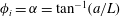
where the conical swirl number,
 $\unicode[STIX]{x1D70E}_{c}$
, is described in appendix A. In the above,
$\unicode[STIX]{x1D70E}_{c}$
, is described in appendix A. In the above,
 $B$
,
$B$
,
 $H$
and
$H$
and
 $p$
represent the angular momentum, stagnation head and pressure, respectively. In addition, we find it useful to associate the cylindrical radii
$p$
represent the angular momentum, stagnation head and pressure, respectively. In addition, we find it useful to associate the cylindrical radii
 $r_{\unicode[STIX]{x1D719}}$
and
$r_{\unicode[STIX]{x1D719}}$
and
 $r_{\unicode[STIX]{x1D6FC}}$
with the zenith angles
$r_{\unicode[STIX]{x1D6FC}}$
with the zenith angles
 $\unicode[STIX]{x1D719}$
and
$\unicode[STIX]{x1D719}$
and
 $\unicode[STIX]{x1D6FC}$
, where
$\unicode[STIX]{x1D6FC}$
, where
 $r_{\unicode[STIX]{x1D6FC}}$
denotes the horizontal distance from the cone axis to the inclined wall. This enables us to define the horizontal radial fraction in any axial plane using
$r_{\unicode[STIX]{x1D6FC}}$
denotes the horizontal distance from the cone axis to the inclined wall. This enables us to define the horizontal radial fraction in any axial plane using
 $$\begin{eqnarray}X_{\unicode[STIX]{x1D719}}={\displaystyle \frac{r_{\unicode[STIX]{x1D719}}}{r_{\unicode[STIX]{x1D6FC}}}}={\displaystyle \frac{\tan \unicode[STIX]{x1D719}}{\tan \unicode[STIX]{x1D6FC}}}.\end{eqnarray}$$
Accordingly, the locally normalized radial distance corresponding to the open outflow fraction may be expressed as
 $X_{\unicode[STIX]{x1D6FD}}=r_{\unicode[STIX]{x1D6FD}}/r_{\unicode[STIX]{x1D6FC}}=b/a$
at any axial elevation
$X_{\unicode[STIX]{x1D6FD}}=r_{\unicode[STIX]{x1D6FD}}/r_{\unicode[STIX]{x1D6FC}}=b/a$
at any axial elevation
 $z$
. Furthermore, owing to the geometric similarity at fixed divergence angle, the length
$z$
. Furthermore, owing to the geometric similarity at fixed divergence angle, the length
 $L$
does not appear in a judiciously normalized system, where it may be readily supplanted by
$L$
does not appear in a judiciously normalized system, where it may be readily supplanted by
 $l=\cot \unicode[STIX]{x1D6FC}$
.
$l=\cot \unicode[STIX]{x1D6FC}$
.
3 Solution
3.1 Bragg–Hawthorne equation
Euler’s equation can be written as
 $\unicode[STIX]{x1D735}H-\boldsymbol{u}\times \unicode[STIX]{x1D74E}=0$
, where
$\unicode[STIX]{x1D735}H-\boldsymbol{u}\times \unicode[STIX]{x1D74E}=0$
, where
 $H=p+u^{2}/2$
represents the dimensionless fluid head. For a given streamfunction,
$H=p+u^{2}/2$
represents the dimensionless fluid head. For a given streamfunction,
 $\unicode[STIX]{x1D713}(R,\unicode[STIX]{x1D719})$
, the radial and zenith velocities may be expressed as
$\unicode[STIX]{x1D713}(R,\unicode[STIX]{x1D719})$
, the radial and zenith velocities may be expressed as
 $$\begin{eqnarray}u_{R}={\displaystyle \frac{1}{R^{2}\sin \unicode[STIX]{x1D719}}}{\displaystyle \frac{\unicode[STIX]{x2202}\unicode[STIX]{x1D713}}{\unicode[STIX]{x2202}\unicode[STIX]{x1D719}}};\quad u_{\unicode[STIX]{x1D719}}=-{\displaystyle \frac{1}{R\sin \unicode[STIX]{x1D719}}}{\displaystyle \frac{\unicode[STIX]{x2202}\unicode[STIX]{x1D713}}{\unicode[STIX]{x2202}R}}.\end{eqnarray}$$
Based on the
 $\unicode[STIX]{x1D703}$
-momentum equation, we group
$\unicode[STIX]{x1D703}$
-momentum equation, we group
 $u_{\unicode[STIX]{x1D703}}R\sin \unicode[STIX]{x1D719}$
and convert (2.4) into
$u_{\unicode[STIX]{x1D703}}R\sin \unicode[STIX]{x1D719}$
and convert (2.4) into
 $$\begin{eqnarray}u_{R}{\displaystyle \frac{\unicode[STIX]{x2202}}{\unicode[STIX]{x2202}R}}(u_{\unicode[STIX]{x1D703}}R\sin \unicode[STIX]{x1D719})+{\displaystyle \frac{u_{\unicode[STIX]{x1D719}}}{R}}{\displaystyle \frac{\unicode[STIX]{x2202}}{\unicode[STIX]{x2202}\unicode[STIX]{x1D719}}}(u_{\unicode[STIX]{x1D703}}R\sin \unicode[STIX]{x1D719})=0.\end{eqnarray}$$
The resulting material derivative directly leads to the tangential velocity,
 $$\begin{eqnarray}u_{\unicode[STIX]{x1D703}}R\sin \unicode[STIX]{x1D719}=B(\unicode[STIX]{x1D713})\quad \text{or}\quad u_{\unicode[STIX]{x1D703}}={\displaystyle \frac{B(\unicode[STIX]{x1D713})}{R\sin \unicode[STIX]{x1D719}}},\end{eqnarray}$$
where the tangential angular momentum,
 $B(\unicode[STIX]{x1D713})$
, is yet to be determined. Using the free vortex relation for the tangential velocity,
$B(\unicode[STIX]{x1D713})$
, is yet to be determined. Using the free vortex relation for the tangential velocity,
 $B(\unicode[STIX]{x1D713})$
may be linked to the radial vorticity,
$B(\unicode[STIX]{x1D713})$
may be linked to the radial vorticity,
 $\unicode[STIX]{x1D714}_{R}$
. By substituting
$\unicode[STIX]{x1D714}_{R}$
. By substituting
 $u_{\unicode[STIX]{x1D703}}$
into (2.5), we retrieve
$u_{\unicode[STIX]{x1D703}}$
into (2.5), we retrieve
 $$\begin{eqnarray}\unicode[STIX]{x1D714}_{R}={\displaystyle \frac{1}{R^{2}\sin \unicode[STIX]{x1D719}}}{\displaystyle \frac{\text{d}B}{\text{d}\unicode[STIX]{x1D713}}}{\displaystyle \frac{\unicode[STIX]{x2202}\unicode[STIX]{x1D713}}{\unicode[STIX]{x2202}\unicode[STIX]{x1D719}}},\end{eqnarray}$$
where the derivative with respect to
 $\unicode[STIX]{x1D713}$
is used in view of
$\unicode[STIX]{x1D713}$
is used in view of
 $B=B(\unicode[STIX]{x1D713})$
. Next, the tangential vorticity may be extracted from the
$B=B(\unicode[STIX]{x1D713})$
. Next, the tangential vorticity may be extracted from the
 $\unicode[STIX]{x1D719}$
-momentum equation. Transforming
$\unicode[STIX]{x1D719}$
-momentum equation. Transforming
 $\unicode[STIX]{x1D735}H-\boldsymbol{u}\times \unicode[STIX]{x1D74E}=0$
into scalar form, we segregate the
$\unicode[STIX]{x1D735}H-\boldsymbol{u}\times \unicode[STIX]{x1D74E}=0$
into scalar form, we segregate the
 $\unicode[STIX]{x1D719}$
-component and write
$\unicode[STIX]{x1D719}$
-component and write
 $$\begin{eqnarray}{\displaystyle \frac{1}{R}}{\displaystyle \frac{\text{d}H}{\text{d}\unicode[STIX]{x1D713}}}{\displaystyle \frac{\unicode[STIX]{x2202}\unicode[STIX]{x1D713}}{\unicode[STIX]{x2202}\unicode[STIX]{x1D719}}}+{\displaystyle \frac{1}{R^{2}\sin \unicode[STIX]{x1D719}}}\unicode[STIX]{x1D714}_{\unicode[STIX]{x1D703}}-{\displaystyle \frac{B(\unicode[STIX]{x1D713})}{R\sin \unicode[STIX]{x1D719}}}\left({\displaystyle \frac{1}{R^{2}\sin \unicode[STIX]{x1D719}}}{\displaystyle \frac{\text{d}B}{\text{d}\unicode[STIX]{x1D713}}}{\displaystyle \frac{\unicode[STIX]{x2202}\unicode[STIX]{x1D713}}{\unicode[STIX]{x2202}\unicode[STIX]{x1D719}}}\right)=0.\end{eqnarray}$$
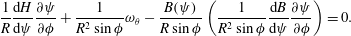
This expression may be considerably simplified and rearranged into
 $$\begin{eqnarray}{\displaystyle \frac{\unicode[STIX]{x1D714}_{\unicode[STIX]{x1D703}}}{R\sin \unicode[STIX]{x1D719}}}={\displaystyle \frac{1}{R^{2}\sin ^{2}\unicode[STIX]{x1D719}}}B(\unicode[STIX]{x1D713}){\displaystyle \frac{\text{d}B}{\text{d}\unicode[STIX]{x1D713}}}-{\displaystyle \frac{\text{d}H}{\text{d}\unicode[STIX]{x1D713}}}.\end{eqnarray}$$
After inserting
 $\unicode[STIX]{x1D714}_{\unicode[STIX]{x1D703}}$
from (2.5) into (3.6), the velocities may be eliminated through (3.1). The outcome is a form of the Bragg–Hawthorne equation in spherical coordinates, namely,
$\unicode[STIX]{x1D714}_{\unicode[STIX]{x1D703}}$
from (2.5) into (3.6), the velocities may be eliminated through (3.1). The outcome is a form of the Bragg–Hawthorne equation in spherical coordinates, namely,
 $$\begin{eqnarray}{\displaystyle \frac{\unicode[STIX]{x2202}^{2}\unicode[STIX]{x1D713}}{\unicode[STIX]{x2202}R^{2}}}+{\displaystyle \frac{\sin \unicode[STIX]{x1D719}}{R^{2}}}{\displaystyle \frac{\unicode[STIX]{x2202}}{\unicode[STIX]{x2202}\unicode[STIX]{x1D719}}}\left({\displaystyle \frac{1}{\sin \unicode[STIX]{x1D719}}}{\displaystyle \frac{\unicode[STIX]{x2202}\unicode[STIX]{x1D713}}{\unicode[STIX]{x2202}\unicode[STIX]{x1D719}}}\right)=R^{2}\sin ^{2}\unicode[STIX]{x1D719}{\displaystyle \frac{\text{d}H}{\text{d}\unicode[STIX]{x1D713}}}-B(\unicode[STIX]{x1D713}){\displaystyle \frac{\text{d}B}{\text{d}\unicode[STIX]{x1D713}}}.\end{eqnarray}$$
In what follows, the proper choice of
 $B(\unicode[STIX]{x1D713})$
and
$B(\unicode[STIX]{x1D713})$
and
 $H(\unicode[STIX]{x1D713})$
will be instrumental to the solution of (3.7). In order to link
$H(\unicode[STIX]{x1D713})$
will be instrumental to the solution of (3.7). In order to link
 $B$
and
$B$
and
 $H$
, we consider the inlet condition where the tangential velocity enters at an average velocity of
$H$
, we consider the inlet condition where the tangential velocity enters at an average velocity of
 $U$
. Based on the tangential momentum equation, we have
$U$
. Based on the tangential momentum equation, we have
 $$\begin{eqnarray}u_{\unicode[STIX]{x1D703}}R\sin \unicode[STIX]{x1D719}=B(\unicode[STIX]{x1D713}),\end{eqnarray}$$
where
 $B$
remains constant along a streamline. Next we differentiate (2.7) and (3.8) with respect to
$B$
remains constant along a streamline. Next we differentiate (2.7) and (3.8) with respect to
 $R\sin \unicode[STIX]{x1D719}$
to obtain, at the top section of the cone,
$R\sin \unicode[STIX]{x1D719}$
to obtain, at the top section of the cone,
 $$\begin{eqnarray}{\displaystyle \frac{\text{d}B}{\text{d}(R\sin \unicode[STIX]{x1D719})}}=1;\quad {\displaystyle \frac{\text{d}\unicode[STIX]{x1D713}}{\text{d}(R\sin \unicode[STIX]{x1D719})}}={\displaystyle \frac{R\sin \unicode[STIX]{x1D719}}{\unicode[STIX]{x03C0}\unicode[STIX]{x1D70E}_{c}}}.\end{eqnarray}$$
A combination of these two expressions leads to
 $$\begin{eqnarray}B{\displaystyle \frac{\text{d}B}{\text{d}\unicode[STIX]{x1D713}}}=\unicode[STIX]{x03C0}\unicode[STIX]{x1D70E}_{c}\equiv \unicode[STIX]{x1D705}_{c}=\text{const.}\end{eqnarray}$$
This relation grants the tangential velocity the freedom to vary with the streamfunction. Assuming a constant inlet velocity, we have
 $\text{d}H/\text{d}\unicode[STIX]{x1D713}=0$
. Furthermore, in view of the flow being isentropic, the total enthalpy variation reduces to that of the stagnation pressure head (Bragg & Hawthorne Reference Bragg and Hawthorne1950). These substitutions into the Bragg–Hawthorne equation lead to a substantially more compact form, namely,
$\text{d}H/\text{d}\unicode[STIX]{x1D713}=0$
. Furthermore, in view of the flow being isentropic, the total enthalpy variation reduces to that of the stagnation pressure head (Bragg & Hawthorne Reference Bragg and Hawthorne1950). These substitutions into the Bragg–Hawthorne equation lead to a substantially more compact form, namely,
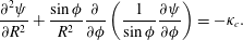 $$\begin{eqnarray}{\displaystyle \frac{\unicode[STIX]{x2202}^{2}\unicode[STIX]{x1D713}}{\unicode[STIX]{x2202}R^{2}}}+{\displaystyle \frac{\sin \unicode[STIX]{x1D719}}{R^{2}}}{\displaystyle \frac{\unicode[STIX]{x2202}}{\unicode[STIX]{x2202}\unicode[STIX]{x1D719}}}\left({\displaystyle \frac{1}{\sin \unicode[STIX]{x1D719}}}{\displaystyle \frac{\unicode[STIX]{x2202}\unicode[STIX]{x1D713}}{\unicode[STIX]{x2202}\unicode[STIX]{x1D719}}}\right)=-\unicode[STIX]{x1D705}_{c}.\end{eqnarray}$$
3.2 Streamfunction and velocities
In seeking an exact solution, we posit
 $\unicode[STIX]{x1D713}=R^{2}G(\unicode[STIX]{x1D719})$
and, pursuant to the work detailed in § B.1, we obtain
$\unicode[STIX]{x1D713}=R^{2}G(\unicode[STIX]{x1D719})$
and, pursuant to the work detailed in § B.1, we obtain
 $$\begin{eqnarray}\unicode[STIX]{x1D713}={\textstyle \frac{1}{2}}\unicode[STIX]{x1D705}_{c}R^{2}\sin ^{2}\unicode[STIX]{x1D719}(\unicode[STIX]{x1D706}-\ln \unicode[STIX]{x1D6F7}+\csc \unicode[STIX]{x1D719}\cot \unicode[STIX]{x1D719}-\csc ^{2}\unicode[STIX]{x1D719}),\end{eqnarray}$$
where
 $$\begin{eqnarray}\unicode[STIX]{x1D706}=\csc ^{2}\unicode[STIX]{x1D6FC}-\csc \unicode[STIX]{x1D6FC}\cot \unicode[STIX]{x1D6FC}+\ln \unicode[STIX]{x1D6F7}_{\unicode[STIX]{x1D6FC}}=\unicode[STIX]{x1D6F7}_{\unicode[STIX]{x1D6FC}}\csc \unicode[STIX]{x1D6FC}+\ln \unicode[STIX]{x1D6F7}_{\unicode[STIX]{x1D6FC}}\end{eqnarray}$$
 $$\begin{eqnarray}\unicode[STIX]{x1D6F7}\equiv \tan ({\textstyle \frac{1}{2}}\unicode[STIX]{x1D719});\quad \unicode[STIX]{x1D6F7}_{\unicode[STIX]{x1D6FC}}\equiv \tan ({\textstyle \frac{1}{2}}\unicode[STIX]{x1D6FC}).\end{eqnarray}$$
The corresponding velocities become
 $$\begin{eqnarray}\displaystyle & \displaystyle u_{R}=\unicode[STIX]{x1D705}_{c}[(\unicode[STIX]{x1D706}-\ln \unicode[STIX]{x1D6F7})\cos \unicode[STIX]{x1D719}-1], & \displaystyle\end{eqnarray}$$
 $$\begin{eqnarray}\displaystyle & \displaystyle u_{\unicode[STIX]{x1D719}}=\unicode[STIX]{x1D705}_{c}[(\ln \unicode[STIX]{x1D6F7}-\unicode[STIX]{x1D706})\sin \unicode[STIX]{x1D719}+\unicode[STIX]{x1D6F7}] & \displaystyle\end{eqnarray}$$
and
 $$\begin{eqnarray}u_{\unicode[STIX]{x1D703}}={\displaystyle \frac{1}{R\sin \unicode[STIX]{x1D719}}}[1+(\unicode[STIX]{x1D705}_{c}R\sin \unicode[STIX]{x1D719})^{2}(\unicode[STIX]{x1D706}-\ln \unicode[STIX]{x1D6F7}-\unicode[STIX]{x1D6F7}\csc \unicode[STIX]{x1D719})]^{1/2}.\end{eqnarray}$$
Compared to the inviscid model of Vyas & Majdalani (Reference Vyas and Majdalani2006), the tangential velocity obtained using this approach retains the free vortex form and, as such, the inverse variation with the distance from the axis of rotation
 ${\sim}(R\sin \unicode[STIX]{x1D719})^{-1}$
. Additionally, (3.17) exhibits a crucial dependence on the inlet velocity profile and the spatially varying streamfunction. It can therefore be seen that the characteristic features of this procedure consist of, first, retaining the spatial dependence granted by the streamfunction and, second, accounting for a specific axial injection profile at entry.
${\sim}(R\sin \unicode[STIX]{x1D719})^{-1}$
. Additionally, (3.17) exhibits a crucial dependence on the inlet velocity profile and the spatially varying streamfunction. It can therefore be seen that the characteristic features of this procedure consist of, first, retaining the spatial dependence granted by the streamfunction and, second, accounting for a specific axial injection profile at entry.
At this stage, using the subscript ‘BI’ to denote the model by Bloor & Ingham (Reference Bloor and Ingham1987), one may write
 $$\begin{eqnarray}\unicode[STIX]{x1D713}_{BI}={\textstyle \frac{1}{2}}\unicode[STIX]{x1D705}_{c}R^{2}\sin ^{2}\unicode[STIX]{x1D719}[\unicode[STIX]{x1D706}_{BI}-\ln ({\textstyle \frac{1}{2}}\tan \unicode[STIX]{x1D719})+\csc \unicode[STIX]{x1D719}\cot \unicode[STIX]{x1D719}-\csc ^{2}\unicode[STIX]{x1D719}],\end{eqnarray}$$
where
 $\unicode[STIX]{x1D706}_{BI}\equiv \csc ^{2}\unicode[STIX]{x1D6FC}-\cot \unicode[STIX]{x1D6FC}\csc \unicode[STIX]{x1D6FC}+\ln [(\tan \unicode[STIX]{x1D6FC})/2]$
. Note that for small cone angles, (3.18) may be recovered asymptotically from (3.12) using successively imposed small-angle approximations,
$\unicode[STIX]{x1D706}_{BI}\equiv \csc ^{2}\unicode[STIX]{x1D6FC}-\cot \unicode[STIX]{x1D6FC}\csc \unicode[STIX]{x1D6FC}+\ln [(\tan \unicode[STIX]{x1D6FC})/2]$
. Note that for small cone angles, (3.18) may be recovered asymptotically from (3.12) using successively imposed small-angle approximations,
 $\tan (\unicode[STIX]{x1D719}/2)\approx \unicode[STIX]{x1D719}/2\approx (\tan \unicode[STIX]{x1D719})/2$
. Although the dual displacement of the
$\tan (\unicode[STIX]{x1D719}/2)\approx \unicode[STIX]{x1D719}/2\approx (\tan \unicode[STIX]{x1D719})/2$
. Although the dual displacement of the
 $1/2$
in the streamfunction may seem negligible at first, it can be shown to have a significant impact on the subsequent flow properties, especially for large cone angles.
$1/2$
in the streamfunction may seem negligible at first, it can be shown to have a significant impact on the subsequent flow properties, especially for large cone angles.
3.3 Equivalent cylindrical polar values
In the interest of clarity, our expressions are transformed into their polar cylindrical equivalents. The switch between spherical and cylindrical coordinates follows the standard transformation matrix (§ B.3). By substituting the values for the radial and zenith velocities, the radial and axial velocities in a cylindrical reference frame emerge. Thus, the streamfunction and velocities may be collapsed into
 $$\begin{eqnarray}u_{r}=-\unicode[STIX]{x1D705}_{c}\unicode[STIX]{x1D6F7};\quad u_{z}=\unicode[STIX]{x1D705}_{c}(\unicode[STIX]{x1D706}-\ln \unicode[STIX]{x1D6F7}-1).\end{eqnarray}$$
To convert the streamfunction and velocities into cylindrical coordinates, we employ
 $R=\sqrt{r^{2}+z^{2}}$
,
$R=\sqrt{r^{2}+z^{2}}$
,
 $\sin \unicode[STIX]{x1D719}=r/R$
,
$\sin \unicode[STIX]{x1D719}=r/R$
,
 $\cos \unicode[STIX]{x1D719}=z/R$
, and
$\cos \unicode[STIX]{x1D719}=z/R$
, and
 $\unicode[STIX]{x1D719}=\tan ^{-1}(r/z)$
. These relations yield
$\unicode[STIX]{x1D719}=\tan ^{-1}(r/z)$
. These relations yield
 $$\begin{eqnarray}\displaystyle & \displaystyle \unicode[STIX]{x1D713}={\textstyle \frac{1}{2}}\unicode[STIX]{x1D705}_{c}r^{2}\left(\unicode[STIX]{x1D706}-\ln Z-Z\sqrt{1+\unicode[STIX]{x1D701}^{2}}\right), & \displaystyle\end{eqnarray}$$
 $$\begin{eqnarray}\displaystyle & \displaystyle u_{R}=\unicode[STIX]{x1D705}_{c}[\unicode[STIX]{x1D701}(\unicode[STIX]{x1D706}-\ln Z)(1+\unicode[STIX]{x1D701}^{2})^{-1/2}-1], & \displaystyle\end{eqnarray}$$
 $$\begin{eqnarray}\displaystyle & \displaystyle u_{\unicode[STIX]{x1D719}}=-\unicode[STIX]{x1D705}_{c}[(\unicode[STIX]{x1D706}-\ln Z)(1+\unicode[STIX]{x1D701}^{2})^{-1/2}-Z], & \displaystyle\end{eqnarray}$$
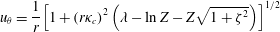 $$\begin{eqnarray}\displaystyle & \displaystyle u_{\unicode[STIX]{x1D703}}=\frac{1}{r}\left[1+(r\unicode[STIX]{x1D705}_{c})^{2}\left(\unicode[STIX]{x1D706}-\ln Z-Z\sqrt{1+\unicode[STIX]{x1D701}^{2}}\right)\right]^{1/2} & \displaystyle\end{eqnarray}$$
and
 $$\begin{eqnarray}u_{r}=-\unicode[STIX]{x1D705}_{c}Z;\quad u_{z}=\unicode[STIX]{x1D705}_{c}(\unicode[STIX]{x1D706}-\ln Z-1),\end{eqnarray}$$
where the dimensionless variables
 $\unicode[STIX]{x1D701}$
and
$\unicode[STIX]{x1D701}$
and
 $Z$
stand for
$Z$
stand for
 $z/r$
and
$z/r$
and
 $\sqrt{1+\unicode[STIX]{x1D701}^{2}}-\unicode[STIX]{x1D701}$
, respectively.
$\sqrt{1+\unicode[STIX]{x1D701}^{2}}-\unicode[STIX]{x1D701}$
, respectively.
4 Results and discussion
4.1 Mantle locations
One of the earliest mentions of the term ‘mantle’ in connection with cyclone separators dates back to Bradley and Pulling (Reference Bradley and Pulling1959; Reference Bradley1965). In this context, Bradley (Reference Bradley1965) defines the mantle as the locus of zero vertical velocity. This locus is specified by the angle at which either
 $u_{R}$
or
$u_{R}$
or
 $u_{z}$
vanishes. Consequently, two mantle inclinations may be defined in a conical chamber as a function of the zenith angle
$u_{z}$
vanishes. Consequently, two mantle inclinations may be defined in a conical chamber as a function of the zenith angle
 $\unicode[STIX]{x1D719}$
. The first,
$\unicode[STIX]{x1D719}$
. The first,
 $\unicode[STIX]{x1D6FD}_{R}$
, corresponds to the location where
$\unicode[STIX]{x1D6FD}_{R}$
, corresponds to the location where
 $u_{R}$
vanishes, and the second coincides with the angle,
$u_{R}$
vanishes, and the second coincides with the angle,
 $\unicode[STIX]{x1D6FD}_{z}$
, where
$\unicode[STIX]{x1D6FD}_{z}$
, where
 $u_{z}=0$
. These can be obtained sequentially from
$u_{z}=0$
. These can be obtained sequentially from
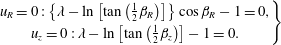 $$\begin{eqnarray}\left.\begin{array}{@{}c@{}}\displaystyle u_{R}=0:\left\{\unicode[STIX]{x1D706}-\ln \left[\tan \left({\textstyle \frac{1}{2}}\unicode[STIX]{x1D6FD}_{R}\right)\right]\right\}\cos \unicode[STIX]{x1D6FD}_{R}-1=0,\\ \displaystyle u_{z}=0:\unicode[STIX]{x1D706}-\ln \left[\tan \left({\textstyle \frac{1}{2}}\unicode[STIX]{x1D6FD}_{z}\right)\right]-1=0.\end{array}\right\}\end{eqnarray}$$
In order to determine the mantle location asymptotically, we first consider the behaviour of the radial velocity
 $u_{R}$
and its corresponding cylindrical velocity,
$u_{R}$
and its corresponding cylindrical velocity,
 $u_{z}$
, as these components direct the flow into and out of the cyclonic chamber. In theory, the two mantles are located where
$u_{z}$
, as these components direct the flow into and out of the cyclonic chamber. In theory, the two mantles are located where
 $u_{R}=0$
and
$u_{R}=0$
and
 $u_{z}=0$
, respectively, thus defining two conical surfaces along which the flow switches polarity between a downward and an upward spiral. Similar experimental and numerical patterns are reported by Pervov (Reference Pervov1974), Luo et al. (Reference Luo, Deng, Xu, Yu and Xiong1989), Zhou & Soo (Reference Zhou and Soo1990), Peng et al. (Reference Peng, Hoffmann, Boot, Udding, Dries, Ekker and Kater2002) and Hu et al. (Reference Hu, Zhou, Zhang and Shi2005). Because
$u_{z}=0$
, respectively, thus defining two conical surfaces along which the flow switches polarity between a downward and an upward spiral. Similar experimental and numerical patterns are reported by Pervov (Reference Pervov1974), Luo et al. (Reference Luo, Deng, Xu, Yu and Xiong1989), Zhou & Soo (Reference Zhou and Soo1990), Peng et al. (Reference Peng, Hoffmann, Boot, Udding, Dries, Ekker and Kater2002) and Hu et al. (Reference Hu, Zhou, Zhang and Shi2005). Because
 $u_{R}$
or
$u_{R}$
or
 $u_{z}$
appear as functions of the zenith angle
$u_{z}$
appear as functions of the zenith angle
 $\unicode[STIX]{x1D719}$
, we solve for the root of
$\unicode[STIX]{x1D719}$
, we solve for the root of
 $u_{R}=0$
and
$u_{R}=0$
and
 $u_{z}=0$
, and call these inclination angles
$u_{z}=0$
, and call these inclination angles
 $\unicode[STIX]{x1D6FD}_{R}$
and
$\unicode[STIX]{x1D6FD}_{R}$
and
 $\unicode[STIX]{x1D6FD}_{z}$
, respectively. Based on (4.1), we set
$\unicode[STIX]{x1D6FD}_{z}$
, respectively. Based on (4.1), we set
 $1-\unicode[STIX]{x1D706}\cos \unicode[STIX]{x1D6FD}_{R}+\ln \unicode[STIX]{x1D6F7}_{\unicode[STIX]{x1D6FD}_{R}}\cos \unicode[STIX]{x1D6FD}_{R}=0$
and
$1-\unicode[STIX]{x1D706}\cos \unicode[STIX]{x1D6FD}_{R}+\ln \unicode[STIX]{x1D6F7}_{\unicode[STIX]{x1D6FD}_{R}}\cos \unicode[STIX]{x1D6FD}_{R}=0$
and
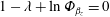 $1-\unicode[STIX]{x1D706}+\ln \unicode[STIX]{x1D6F7}_{\unicode[STIX]{x1D6FD}_{z}}=0$
, where
$1-\unicode[STIX]{x1D706}+\ln \unicode[STIX]{x1D6F7}_{\unicode[STIX]{x1D6FD}_{z}}=0$
, where
 $\unicode[STIX]{x1D6F7}_{\unicode[STIX]{x1D6FD}_{R}}=\tan (\unicode[STIX]{x1D6FD}_{R}/2)$
and
$\unicode[STIX]{x1D6F7}_{\unicode[STIX]{x1D6FD}_{R}}=\tan (\unicode[STIX]{x1D6FD}_{R}/2)$
and
 $\unicode[STIX]{x1D6F7}_{\unicode[STIX]{x1D6FD}_{z}}=\tan (\unicode[STIX]{x1D6FD}_{z}/2)$
. We then use a MacLaurin series expansion to extract
$\unicode[STIX]{x1D6F7}_{\unicode[STIX]{x1D6FD}_{z}}=\tan (\unicode[STIX]{x1D6FD}_{z}/2)$
. We then use a MacLaurin series expansion to extract
 $$\begin{eqnarray}\left.\begin{array}{@{}c@{}}\displaystyle u_{R}=0:1-\unicode[STIX]{x1D706}+\ln \left({\textstyle \frac{1}{2}}\unicode[STIX]{x1D6FD}_{R}\right)+\left({\textstyle \frac{1}{2}}\unicode[STIX]{x1D6FD}_{R}\right)^{2}\left({\textstyle \frac{1}{3}}+2\unicode[STIX]{x1D706}+2\ln 2\right)+\cdots =0,\\ \displaystyle u_{z}=0:1-\unicode[STIX]{x1D706}+\ln \left({\textstyle \frac{1}{2}}\unicode[STIX]{x1D6FD}_{z}\right)+{\textstyle \frac{1}{12}}\unicode[STIX]{x1D6FD}_{z}^{2}+\cdots =0.\end{array}\right\}\end{eqnarray}$$
In actuality, of the twelve algebraic roots that emerge for
 $\unicode[STIX]{x1D6FD}_{R}$
, only two are meaningful, namely,
$\unicode[STIX]{x1D6FD}_{R}$
, only two are meaningful, namely,
 $$\begin{eqnarray}\tilde{\unicode[STIX]{x1D6FD}}_{R}=\left\{\begin{array}{@{}ll@{}}\displaystyle \frac{\sqrt{-\text{pln}[4(\unicode[STIX]{x1D706}+\ln 2+{\textstyle \frac{1}{6}})\text{e}^{2(\unicode[STIX]{x1D706}-1)}]}}{\sqrt{\unicode[STIX]{x1D706}+\ln 2+{\textstyle \frac{1}{6}}}}, & 0<\unicode[STIX]{x1D6FC}\leqslant \unicode[STIX]{x1D6FC}_{0},\\ \displaystyle \frac{\sqrt{\text{pln}[4(\unicode[STIX]{x1D706}+\ln 2+{\textstyle \frac{1}{6}})\text{e}^{2(\unicode[STIX]{x1D706}-1)}]}}{\sqrt{\unicode[STIX]{x1D706}+\ln 2+{\textstyle \frac{1}{6}}}}, & \displaystyle \unicode[STIX]{x1D6FC}_{0}<\unicode[STIX]{x1D6FC}<\frac{1}{2}\unicode[STIX]{x03C0},\end{array}\right.\end{eqnarray}$$
where
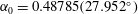 $\unicode[STIX]{x1D6FC}_{0}=0.48785(27.952^{\circ })$
, with the tilde denoting an asymptotic approximation. Fortuitously, it may be shown that the piecewise representation in (4.3) may be collapsed into a single, uniformly valid expression for the mantle location, namely,
$\unicode[STIX]{x1D6FC}_{0}=0.48785(27.952^{\circ })$
, with the tilde denoting an asymptotic approximation. Fortuitously, it may be shown that the piecewise representation in (4.3) may be collapsed into a single, uniformly valid expression for the mantle location, namely,
 $$\begin{eqnarray}\tilde{\unicode[STIX]{x1D6FD}}_{R}=\sqrt{\frac{\text{pln}[4(\unicode[STIX]{x1D706}+\ln 2+{\textstyle \frac{1}{6}})\text{e}^{2(\unicode[STIX]{x1D706}-1)}]}{\unicode[STIX]{x1D706}+\ln 2+{\textstyle \frac{1}{6}}}}=\frac{\unicode[STIX]{x1D6FC}}{\sqrt{\text{e}}}-\left(\frac{1}{3}-\frac{5}{24}\text{e}+\frac{1}{2}\ln \unicode[STIX]{x1D6FC}\right)\left(\frac{\unicode[STIX]{x1D6FC}}{\sqrt{\text{e}}}\right)^{3}+O(\unicode[STIX]{x1D6FC}^{5}\ln \unicode[STIX]{x1D6FC})\end{eqnarray}$$
and so, using a superscript to denote the asymptotic expansion order, we have
 $$\begin{eqnarray}\tilde{\unicode[STIX]{x1D6FD}}_{R}^{(2)}\approx 0.606531\unicode[STIX]{x1D6FC}+0.0519838\unicode[STIX]{x1D6FC}^{3}-0.111565\unicode[STIX]{x1D6FC}^{3}\ln \unicode[STIX]{x1D6FC}.\end{eqnarray}$$
By repeating this process for
 $\unicode[STIX]{x1D6FD}_{z}=2\arctan [\exp (\unicode[STIX]{x1D706}-1)]$
, twelve algebraic roots may be retrieved, but of these only one proves to be physical, specifically,
$\unicode[STIX]{x1D6FD}_{z}=2\arctan [\exp (\unicode[STIX]{x1D706}-1)]$
, twelve algebraic roots may be retrieved, but of these only one proves to be physical, specifically,
 $$\begin{eqnarray}\tilde{\unicode[STIX]{x1D6FD}}_{z}=\sqrt{6\,\text{pln}[{\textstyle \frac{2}{3}}\text{e}^{2(\unicode[STIX]{x1D706}-1)}]}=\frac{\unicode[STIX]{x1D6FC}}{\sqrt{\text{e}}}+\frac{5\text{e}-2}{24}\left(\frac{\unicode[STIX]{x1D6FC}}{\sqrt{\text{e}}}\right)^{3}+\frac{100-300\text{e}+273\text{e}^{2}}{5760}\left(\frac{\unicode[STIX]{x1D6FC}}{\sqrt{\text{e}}}\right)^{5}+O(\unicode[STIX]{x1D6FC}^{7})\end{eqnarray}$$
and so
 $$\begin{eqnarray}\tilde{\unicode[STIX]{x1D6FD}}_{z}^{(2)}\approx 0.606531\unicode[STIX]{x1D6FC}+0.107766\unicode[STIX]{x1D6FC}^{3}+0.0185508\unicode[STIX]{x1D6FC}^{5}.\end{eqnarray}$$
A comparison between (4.5) and (4.7) reinforces the intrinsic similarity between the asymptotic forms of
 $\tilde{\unicode[STIX]{x1D6FD}}_{z}^{(2)}$
and
$\tilde{\unicode[STIX]{x1D6FD}}_{z}^{(2)}$
and
 $\tilde{\unicode[STIX]{x1D6FD}}_{R}^{(2)}$
, which may be traced back to their basic definitions. Alternatively, instead of using the inclination angle
$\tilde{\unicode[STIX]{x1D6FD}}_{R}^{(2)}$
, which may be traced back to their basic definitions. Alternatively, instead of using the inclination angle
 $\unicode[STIX]{x1D6FD}$
to define the mantle, one may track the mantle vertically using the fraction of the radius
$\unicode[STIX]{x1D6FD}$
to define the mantle, one may track the mantle vertically using the fraction of the radius
 $X_{\unicode[STIX]{x1D6FD}_{R}}$
or
$X_{\unicode[STIX]{x1D6FD}_{R}}$
or
 $X_{\unicode[STIX]{x1D6FD}_{z}}$
corresponding to either
$X_{\unicode[STIX]{x1D6FD}_{z}}$
corresponding to either
 $u_{R}=0$
or
$u_{R}=0$
or
 $u_{z}=0$
. As per (2.11), these are given by
$u_{z}=0$
. As per (2.11), these are given by
 $$\begin{eqnarray}X_{\unicode[STIX]{x1D6FD}_{R}}=\tan \unicode[STIX]{x1D6FD}_{R}/\tan \unicode[STIX]{x1D6FC};\quad X_{\unicode[STIX]{x1D6FD}_{z}}=\tan \unicode[STIX]{x1D6FD}_{z}/\tan \unicode[STIX]{x1D6FC},\end{eqnarray}$$
which can be approximated using
 $$\begin{eqnarray}\tilde{X}_{\unicode[STIX]{x1D6FD}_{R}}=\cot \unicode[STIX]{x1D6FC}\tan \left\{\frac{1+\cos \unicode[STIX]{x1D6FC}\,\text{pln}[4\unicode[STIX]{x1D6F7}_{\unicode[STIX]{x1D6FC}}^{2}\text{e}^{\unicode[STIX]{x1D6F7}_{\unicode[STIX]{x1D6FC}}^{2}-1}({\textstyle \frac{1}{6}}+\ln 2\unicode[STIX]{x1D6F7}_{\unicode[STIX]{x1D6FC}}+\unicode[STIX]{x1D6F7}_{\unicode[STIX]{x1D6FC}}\csc \unicode[STIX]{x1D6FC})]}{1+(1+\cos \unicode[STIX]{x1D6FC})[{\textstyle \frac{1}{6}}+\ln 2\unicode[STIX]{x1D6F7}_{\unicode[STIX]{x1D6FC}}]}\right\}^{1/2}\end{eqnarray}$$
and
 $$\begin{eqnarray}\tilde{X}_{\unicode[STIX]{x1D6FD}_{z}}=\cot \unicode[STIX]{x1D6FC}\tan \left[6\sqrt{\text{pln}\left({\textstyle \frac{2}{3}}\unicode[STIX]{x1D6F7}_{\unicode[STIX]{x1D6FC}}^{2}\text{e}^{\unicode[STIX]{x1D6F7}_{\unicode[STIX]{x1D6FC}}^{2}-1}\right)}\right].\end{eqnarray}$$
In practice, a three-term asymptotic expansion for each of the radial fractions may be conveniently retrieved, specifically,
 $$\begin{eqnarray}\tilde{X}_{\unicode[STIX]{x1D6FD}_{R}}^{(2)}=\frac{1}{\sqrt{\text{e}}}-\frac{\text{e}+4\ln \unicode[STIX]{x1D6FC}}{8\text{e}\sqrt{\text{e}}}\unicode[STIX]{x1D6FC}^{2}\approx 0.606531-0.0758163\unicode[STIX]{x1D6FC}^{2}-0.111565\unicode[STIX]{x1D6FC}^{2}\ln \unicode[STIX]{x1D6FC}\end{eqnarray}$$
and
 $$\begin{eqnarray}\displaystyle \tilde{X}_{\unicode[STIX]{x1D6FD}_{z}}^{(2)} & = & \displaystyle \frac{1}{\sqrt{\text{e}}}+\frac{2-\text{e}}{8\text{e}\sqrt{\text{e}}}\unicode[STIX]{x1D6FC}^{2}+\frac{388+420\text{e}-255\text{e}^{2}}{5760\text{e}^{2}\sqrt{\text{e}}}\unicode[STIX]{x1D6FC}^{4}\nonumber\\ \displaystyle & {\approx} & \displaystyle 0.606531-0.0200338\unicode[STIX]{x1D6FC}^{2}-0.00505237\unicode[STIX]{x1D6FC}^{4}.\end{eqnarray}$$
Equations (4.4) and (4.6) are quite illuminating. In view of the small size of
 $\unicode[STIX]{x1D6FC}\text{e}^{-1/2}$
, a one-term approximation of the mantle location yields
$\unicode[STIX]{x1D6FC}\text{e}^{-1/2}$
, a one-term approximation of the mantle location yields
 $\unicode[STIX]{x1D6FD}_{R}=\unicode[STIX]{x1D6FD}_{z}\approx 0.6065\unicode[STIX]{x1D6FC}$
, which explains the ubiquitous use of
$\unicode[STIX]{x1D6FD}_{R}=\unicode[STIX]{x1D6FD}_{z}\approx 0.6065\unicode[STIX]{x1D6FC}$
, which explains the ubiquitous use of
 $\unicode[STIX]{x1D6FD}_{z}=0.6\unicode[STIX]{x1D6FC}$
, or alternatively,
$\unicode[STIX]{x1D6FD}_{z}=0.6\unicode[STIX]{x1D6FC}$
, or alternatively,
 $X_{\unicode[STIX]{x1D6FD}_{z}}=0.6$
, in several empirical studies of conically shaped cyclone separators. Therein, using
$X_{\unicode[STIX]{x1D6FD}_{z}}=0.6$
, in several empirical studies of conically shaped cyclone separators. Therein, using
 $u_{z}=0$
to define the mantle seems to be preferred, at least from an experimental perspective, over the
$u_{z}=0$
to define the mantle seems to be preferred, at least from an experimental perspective, over the
 $u_{R}=0$
criterion. This is owed in large part to the ease with which the
$u_{R}=0$
criterion. This is owed in large part to the ease with which the
 $u_{z}=0$
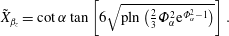
condition may be implemented experimentally, or recreated numerically. According to (4.4), the use of
$u_{z}=0$
condition may be implemented experimentally, or recreated numerically. According to (4.4), the use of
 $\unicode[STIX]{x1D6FD}_{R}=0.6\unicode[STIX]{x1D6FC}$
entails an absolute error that varies between 0.0066 and
$\unicode[STIX]{x1D6FD}_{R}=0.6\unicode[STIX]{x1D6FC}$
entails an absolute error that varies between 0.0066 and
 $0.11^{\circ }$
for
$0.11^{\circ }$
for
 $1\leqslant \unicode[STIX]{x1D6FC}\leqslant 60^{\circ }$
. In practice, the 60 % mantle inclination is repeatedly reported in several independent investigations, including those by Bradley & Pulling (Reference Bradley and Pulling1959), Pervov (Reference Pervov1974), Dabir & Petty (Reference Dabir and Petty1986), Hoekstra et al. (Reference Hoekstra, Derksen and van den Akker1999) and Chesnokov, Bauman & Flisyuk (Reference Chesnokov, Bauman and Flisyuk2006).
$1\leqslant \unicode[STIX]{x1D6FC}\leqslant 60^{\circ }$
. In practice, the 60 % mantle inclination is repeatedly reported in several independent investigations, including those by Bradley & Pulling (Reference Bradley and Pulling1959), Pervov (Reference Pervov1974), Dabir & Petty (Reference Dabir and Petty1986), Hoekstra et al. (Reference Hoekstra, Derksen and van den Akker1999) and Chesnokov, Bauman & Flisyuk (Reference Chesnokov, Bauman and Flisyuk2006).

Figure 3. Mantle inclination angle versus
 $\unicode[STIX]{x1D6FC}$
as predicted by either (a)
$\unicode[STIX]{x1D6FC}$
as predicted by either (a)
 $\unicode[STIX]{x1D6FD}_{R}$
(——) and
$\unicode[STIX]{x1D6FD}_{R}$
(——) and
 $\tilde{\unicode[STIX]{x1D6FD}}_{R}^{(0)}$
(– – –) or (b)
$\tilde{\unicode[STIX]{x1D6FD}}_{R}^{(0)}$
(– – –) or (b)
 $\unicode[STIX]{x1D6FD}_{z}$
(——) and
$\unicode[STIX]{x1D6FD}_{z}$
(——) and
 $\tilde{\unicode[STIX]{x1D6FD}}_{z}^{(2)}$
(– – –). Also shown is the connection between these solutions and
$\tilde{\unicode[STIX]{x1D6FD}}_{z}^{(2)}$
(– – –). Also shown is the connection between these solutions and
 $\unicode[STIX]{x1D706}$
(— ⋅ —).
$\unicode[STIX]{x1D706}$
(— ⋅ —).
To further characterize the mantle inclination, the functional dependence of
 $\unicode[STIX]{x1D6FD}_{R}$
and
$\unicode[STIX]{x1D6FD}_{R}$
and
 $\unicode[STIX]{x1D6FD}_{z}$
on
$\unicode[STIX]{x1D6FD}_{z}$
on
 $\unicode[STIX]{x1D6FC}$
is illustrated in figure 3 as well as table 1. Note that
$\unicode[STIX]{x1D6FC}$
is illustrated in figure 3 as well as table 1. Note that
 $\unicode[STIX]{x1D706}$
varies between
$\unicode[STIX]{x1D706}$
varies between
 $-$
4.24 and 1 for
$-$
4.24 and 1 for
 $1\leqslant \unicode[STIX]{x1D6FC}\leqslant 90^{\circ }$
. As for the mantle location, both exact and approximate representations are overlaid and shown to be graphically indiscernible, except when the divergence half-angle approaches the impractical value of
$1\leqslant \unicode[STIX]{x1D6FC}\leqslant 90^{\circ }$
. As for the mantle location, both exact and approximate representations are overlaid and shown to be graphically indiscernible, except when the divergence half-angle approaches the impractical value of
 $90^{\circ }$
. Nonetheless, the error incurred in using
$90^{\circ }$
. Nonetheless, the error incurred in using
 $\unicode[STIX]{x1D6FD}_{R}=0.6\unicode[STIX]{x1D6FC}$
to estimate the mantle location reaches a maximum of
$\unicode[STIX]{x1D6FD}_{R}=0.6\unicode[STIX]{x1D6FC}$
to estimate the mantle location reaches a maximum of
 $0.44^{\circ }$
at
$0.44^{\circ }$
at
 $\unicode[STIX]{x1D6FC}=90^{\circ }$
, unlike the error in
$\unicode[STIX]{x1D6FC}=90^{\circ }$
, unlike the error in
 $\unicode[STIX]{x1D6FD}_{z}$
, which exceeds
$\unicode[STIX]{x1D6FD}_{z}$
, which exceeds
 $1.3^{\circ }$
using
$1.3^{\circ }$
using
 $\tilde{\unicode[STIX]{x1D6FD}}_{z}^{(2)}$
. Instead, the
$\tilde{\unicode[STIX]{x1D6FD}}_{z}^{(2)}$
. Instead, the
 $u_{z}=0$
condition leads to a rather uniform ratio
$u_{z}=0$
condition leads to a rather uniform ratio
 $X_{\unicode[STIX]{x1D6FD}_{z}}$
at any axial station. We conclude that, for divergence half-angles below
$X_{\unicode[STIX]{x1D6FD}_{z}}$
at any axial station. We conclude that, for divergence half-angles below
 $38^{\circ }$
, both
$38^{\circ }$
, both
 $\unicode[STIX]{x1D6FD}_{R}$
and
$\unicode[STIX]{x1D6FD}_{R}$
and
 $\unicode[STIX]{x1D6FD}_{z}$
may be suitably relied on to characterize the mantle, as their predictions in this range fall within 5 % or less. For larger angles, only
$\unicode[STIX]{x1D6FD}_{z}$
may be suitably relied on to characterize the mantle, as their predictions in this range fall within 5 % or less. For larger angles, only
 $\unicode[STIX]{x1D6FD}_{R}$
continues to follow the 60 % of
$\unicode[STIX]{x1D6FD}_{R}$
continues to follow the 60 % of
 $\unicode[STIX]{x1D6FC}$
approximation. These results are clearly reflected in table 1.
$\unicode[STIX]{x1D6FC}$
approximation. These results are clearly reflected in table 1.
Table 1. Properties of the two characteristic mantles at different conical half-angles.

4.2 Streamlines
The streamlines prescribed by (3.20) are shown in figure 4 at four different cone half-angles of
 $30^{\circ }$
,
$30^{\circ }$
,
 $45^{\circ }$
,
$45^{\circ }$
,
 $60^{\circ }$
and
$60^{\circ }$
and
 $75^{\circ }$
. The contour curves represent lines of constant
$75^{\circ }$
. The contour curves represent lines of constant
 $\unicode[STIX]{x1D713}$
, which illustrate the downdraft, bending and updraft regions. Also shown are the mantle inclinations corresponding to
$\unicode[STIX]{x1D713}$
, which illustrate the downdraft, bending and updraft regions. Also shown are the mantle inclinations corresponding to
 $u_{R}=0$
and denoted by
$u_{R}=0$
and denoted by
 $\unicode[STIX]{x1D6FD}_{R}$
. The observed subdivisions of the flow field are consistent with several experimental studies, including those by Shepherd & Lapple (Reference Shepherd and Lapple1939), Stairmand (Reference Stairmand1951), Kelsall (Reference Kelsall1952), Escudier (Reference Escudier1987) and Peng et al. (Reference Peng, Hoffmann, Boot, Udding, Dries, Ekker and Kater2002). Here the dashed lines represent
$\unicode[STIX]{x1D6FD}_{R}$
. The observed subdivisions of the flow field are consistent with several experimental studies, including those by Shepherd & Lapple (Reference Shepherd and Lapple1939), Stairmand (Reference Stairmand1951), Kelsall (Reference Kelsall1952), Escudier (Reference Escudier1987) and Peng et al. (Reference Peng, Hoffmann, Boot, Udding, Dries, Ekker and Kater2002). Here the dashed lines represent
 $\unicode[STIX]{x1D713}_{BI}$
, which clearly deviates from the present solution as
$\unicode[STIX]{x1D713}_{BI}$
, which clearly deviates from the present solution as
 $\unicode[STIX]{x1D6FC}$
is increased. Interestingly, these streamlines appear as though they are entering the conical chamber through the outlet, instead of the inlet, because the small-angle approximation that the Bloor–Ingham solution is based on deteriorates as
$\unicode[STIX]{x1D6FC}$
is increased. Interestingly, these streamlines appear as though they are entering the conical chamber through the outlet, instead of the inlet, because the small-angle approximation that the Bloor–Ingham solution is based on deteriorates as
 $\unicode[STIX]{x1D719}$
is increased. Furthermore, the differences in streamline curvatures translate into deviations in the velocity components. For example, the relative difference between the exact value of
$\unicode[STIX]{x1D719}$
is increased. Furthermore, the differences in streamline curvatures translate into deviations in the velocity components. For example, the relative difference between the exact value of
 $u_{R}$
and its predicted value based on
$u_{R}$
and its predicted value based on
 $\unicode[STIX]{x1D713}_{BI}$
reaches
$\unicode[STIX]{x1D713}_{BI}$
reaches
 $5$
per cent for a cone half-angle of
$5$
per cent for a cone half-angle of
 $28^{\circ }$
.
$28^{\circ }$
.

Figure 4. Flow streamlines for
 $\unicode[STIX]{x1D70E}_{c}=1$
and cone half-angles of (a)
$\unicode[STIX]{x1D70E}_{c}=1$
and cone half-angles of (a)
 $30^{\circ }$
, (b)
$30^{\circ }$
, (b)
 $45^{\circ }$
, (c)
$45^{\circ }$
, (c)
 $60^{\circ }$
and (d)
$60^{\circ }$
and (d)
 $75^{\circ }$
. Here, the present model (——) is compared to the small-angle approximation by Bloor & Ingham (Reference Bloor and Ingham1987) (– – –). Also shown are the corresponding mantle inclinations (— ⋅ —) of
$75^{\circ }$
. Here, the present model (——) is compared to the small-angle approximation by Bloor & Ingham (Reference Bloor and Ingham1987) (– – –). Also shown are the corresponding mantle inclinations (— ⋅ —) of
 $\unicode[STIX]{x1D6FD}_{R}\approx 18^{\circ }$
,
$\unicode[STIX]{x1D6FD}_{R}\approx 18^{\circ }$
,
 $27^{\circ }$
,
$27^{\circ }$
,
 $36^{\circ }$
and
$36^{\circ }$
and
 $45^{\circ }$
, respectively.
$45^{\circ }$
, respectively.
4.3 Spherical radial and zenith velocity distributions
The spherical radial velocity,
 $u_{R}$
, controls the spherical polarity of the flow. Simply put, negative values imply downward motion along the
$u_{R}$
, controls the spherical polarity of the flow. Simply put, negative values imply downward motion along the
 $R$
coordinate whereas positive values correspond to an updraft (figure 1). In figure 4, the direction and location of the flow are specified. The outer vortex is delineated by the region in which
$R$
coordinate whereas positive values correspond to an updraft (figure 1). In figure 4, the direction and location of the flow are specified. The outer vortex is delineated by the region in which
 $u_{R}<0$
, wherein the fluid is transported downwardly in a spiralling fashion. In contrast, the positive
$u_{R}<0$
, wherein the fluid is transported downwardly in a spiralling fashion. In contrast, the positive
 $u_{R}$
region within the inner vortex induces convection of the spinning fluid upwardly and out of the top.
$u_{R}$
region within the inner vortex induces convection of the spinning fluid upwardly and out of the top.
Another feature that may be inferred from
 $u_{R}$
concerns the physicality and behaviour of the spherical radial mantle. This corresponds to the surface of revolution where
$u_{R}$
concerns the physicality and behaviour of the spherical radial mantle. This corresponds to the surface of revolution where
 $u_{R}=0$
. The ensuing mantle inclination remains constant throughout the cone, and this property leads to a constantly changing horizontal location as the axial position is vertically increased. This particular axial shifting is confirmed through (3.21) and may be observed in figure 5, where
$u_{R}=0$
. The ensuing mantle inclination remains constant throughout the cone, and this property leads to a constantly changing horizontal location as the axial position is vertically increased. This particular axial shifting is confirmed through (3.21) and may be observed in figure 5, where
 $u_{R}$
is plotted at either (a) four axial locations or (b) five half-angles, to clearly demarcate the inner and outer vortex regions.
$u_{R}$
is plotted at either (a) four axial locations or (b) five half-angles, to clearly demarcate the inner and outer vortex regions.

Figure 5. Radial and zenith velocity distributions for
 $\unicode[STIX]{x1D70E}_{c}=1$
taken at (a,c) several axial positions for a fixed divergence half-angle of
$\unicode[STIX]{x1D70E}_{c}=1$
taken at (a,c) several axial positions for a fixed divergence half-angle of
 $45^{\circ }$
and (b,d) several half-angles at the top of the cone where
$45^{\circ }$
and (b,d) several half-angles at the top of the cone where
 $z/l=1$
. The four curves in (a,c) correspond to
$z/l=1$
. The four curves in (a,c) correspond to
 $z/l=1$
(——),
$z/l=1$
(——),
 $0.75$
(– – –),
$0.75$
(– – –),
 $0.5$
(— ⋅ —) and
$0.5$
(— ⋅ —) and
 $0.25$
(
$0.25$
(
 $\cdots \cdot$
). The five curves in (b,d) correspond to half-angles of
$\cdots \cdot$
). The five curves in (b,d) correspond to half-angles of
 $\unicode[STIX]{x1D6FC}=75^{\circ }$
(——),
$\unicode[STIX]{x1D6FC}=75^{\circ }$
(——),
 $60^{\circ }$
(– – –),
$60^{\circ }$
(– – –),
 $45^{\circ }$
(— ⋅ —),
$45^{\circ }$
(— ⋅ —),
 $30^{\circ }$
(
$30^{\circ }$
(
 $\cdots \cdots$
) and
$\cdots \cdots$
) and
 $15^{\circ }$
(— ⋅ ⋅ —).
$15^{\circ }$
(— ⋅ ⋅ —).
By inspection of (3.22),
 $u_{\unicode[STIX]{x1D719}}$
is seen to be solely dependent on the zenith angle and the conical swirl number. Being somewhat akin to the radial velocity of the bidirectional vortex considered by Vyas & Majdalani (Reference Vyas and Majdalani2006),
$u_{\unicode[STIX]{x1D719}}$
is seen to be solely dependent on the zenith angle and the conical swirl number. Being somewhat akin to the radial velocity of the bidirectional vortex considered by Vyas & Majdalani (Reference Vyas and Majdalani2006),
 $u_{\unicode[STIX]{x1D719}}$
vanishes at both the core and the side wall. Conversely at
$u_{\unicode[STIX]{x1D719}}$
vanishes at both the core and the side wall. Conversely at
 $\unicode[STIX]{x1D719}=\unicode[STIX]{x1D6FD}_{R}$
or
$\unicode[STIX]{x1D719}=\unicode[STIX]{x1D6FD}_{R}$
or
 $\unicode[STIX]{x1D6FD}_{z}$
, the two complementary velocities
$\unicode[STIX]{x1D6FD}_{z}$
, the two complementary velocities
 $u_{R}$
and
$u_{R}$
and
 $u_{r}$
provide the necessary link between the inner and outer vortex regions, by permitting mass transport across the mantle interface. Because
$u_{r}$
provide the necessary link between the inner and outer vortex regions, by permitting mass transport across the mantle interface. Because
 $u_{R}=0$
at
$u_{R}=0$
at
 $\unicode[STIX]{x1D719}=\unicode[STIX]{x1D6FD}_{R}$
, the connection across the mantle strictly depends on
$\unicode[STIX]{x1D719}=\unicode[STIX]{x1D6FD}_{R}$
, the connection across the mantle strictly depends on
 $u_{\unicode[STIX]{x1D719}}$
. As shown in figure 5, the curves exhibit similar profiles where the variation of
$u_{\unicode[STIX]{x1D719}}$
. As shown in figure 5, the curves exhibit similar profiles where the variation of
 $u_{\unicode[STIX]{x1D719}}$
is shown at four axial cross-sections and five half-angles, respectively. Everywhere between the axis and the wall,
$u_{\unicode[STIX]{x1D719}}$
is shown at four axial cross-sections and five half-angles, respectively. Everywhere between the axis and the wall,
 $u_{\unicode[STIX]{x1D719}}$
retains a negative value that is indicative of inward flow towards the cone axis.
$u_{\unicode[STIX]{x1D719}}$
retains a negative value that is indicative of inward flow towards the cone axis.
It should be remarked that, in the absence of friction, the forced vortex region that characterizes typical cyclonic cores cannot be fully established. Without properly accounting for shearing stresses in the core region,
 $u_{R}$
(and hence
$u_{R}$
(and hence
 $u_{z}$
) becomes unbounded as
$u_{z}$
) becomes unbounded as
 $(\unicode[STIX]{x1D719},r)\rightarrow 0$
. In a viscous medium, a core boundary layer develops around the centreline to the extent of mitigating any divergence in the velocity. One also expects a thin boundary layer to form along the conical wall, in fulfilment of the no slip requirement.
$(\unicode[STIX]{x1D719},r)\rightarrow 0$
. In a viscous medium, a core boundary layer develops around the centreline to the extent of mitigating any divergence in the velocity. One also expects a thin boundary layer to form along the conical wall, in fulfilment of the no slip requirement.
4.4 Tangential and axial velocities
Figure 6 illustrates the behaviour of the swirl and axial velocities compared to the experimental and numerical measurements of Hsieh & Rajamani (Reference Hsieh and Rajamani1988) and Monredon, Hsieh & Rajamani (Reference Monredon, Hsieh and Rajamani1992). We begin with figure 6(a,b), where the swirl velocity in a polar plane is showcased against available experimental and numerical data at two tangential injection velocities. Also shown on the graphs is the free vortex motion given by
 $u_{\unicode[STIX]{x1D703}}=r^{-1}$
. The dimensions of the cyclonic contraptions used by Hsieh & Rajamani (Reference Hsieh and Rajamani1988) and Monredon et al. (Reference Monredon, Hsieh and Rajamani1992) are so analogous that they yield similar values of the modified swirl number
$u_{\unicode[STIX]{x1D703}}=r^{-1}$
. The dimensions of the cyclonic contraptions used by Hsieh & Rajamani (Reference Hsieh and Rajamani1988) and Monredon et al. (Reference Monredon, Hsieh and Rajamani1992) are so analogous that they yield similar values of the modified swirl number
 $\unicode[STIX]{x1D70E}_{c}$
(
$\unicode[STIX]{x1D70E}_{c}$
(
 $\unicode[STIX]{x1D6FC}=10^{\circ },a=0.0375$
m, and
$\unicode[STIX]{x1D6FC}=10^{\circ },a=0.0375$
m, and
 $X_{\unicode[STIX]{x1D6FD}_{R}}\approx 0.6$
). Overall discrepancies observed between theory and measurements or simulations may be attributed in part to the fundamental limitations of an inviscid model. Consistently with the free vortex form of (3.23),
$X_{\unicode[STIX]{x1D6FD}_{R}}\approx 0.6$
). Overall discrepancies observed between theory and measurements or simulations may be attributed in part to the fundamental limitations of an inviscid model. Consistently with the free vortex form of (3.23),
 $u_{\unicode[STIX]{x1D703}}$
becomes unbounded as
$u_{\unicode[STIX]{x1D703}}$
becomes unbounded as
 $r\rightarrow 0$
, and diminishes with the inverse distance from the cone axis. Its axial variation, however, seems to be less pronounced due to its weaker dependence on the streamfunction and the inlet profile. This grants the motion added sensitivity to the inlet conditions, especially when compared to the free vortex model of Vyas & Majdalani (Reference Vyas and Majdalani2006). Therein,
$r\rightarrow 0$
, and diminishes with the inverse distance from the cone axis. Its axial variation, however, seems to be less pronounced due to its weaker dependence on the streamfunction and the inlet profile. This grants the motion added sensitivity to the inlet conditions, especially when compared to the free vortex model of Vyas & Majdalani (Reference Vyas and Majdalani2006). Therein,
 $u_{\unicode[STIX]{x1D703}}=r^{-1}$
is solely dependent on the average inlet velocity. In both models, the strictly inviscid form grows to unbounded levels at the core. By the same token, it fails to accommodate the velocity adherence requirement that must be secured at the wall. This result is actually characteristic of most swirl-dominated frictionless flows; it is ascertained in work by Bloor & Ingham (Reference Bloor and Ingham1987), Harvey (Reference Harvey1962) and Leibovich (Reference Leibovich1978, Reference Leibovich1984). Interestingly, the axial velocities in figure 6(c,d) exhibit similar features to those of
$u_{\unicode[STIX]{x1D703}}=r^{-1}$
is solely dependent on the average inlet velocity. In both models, the strictly inviscid form grows to unbounded levels at the core. By the same token, it fails to accommodate the velocity adherence requirement that must be secured at the wall. This result is actually characteristic of most swirl-dominated frictionless flows; it is ascertained in work by Bloor & Ingham (Reference Bloor and Ingham1987), Harvey (Reference Harvey1962) and Leibovich (Reference Leibovich1978, Reference Leibovich1984). Interestingly, the axial velocities in figure 6(c,d) exhibit similar features to those of
 $u_{R}$
. These are illustrated for
$u_{R}$
. These are illustrated for
 $\unicode[STIX]{x1D70E}_{c}=0.2$
and
$\unicode[STIX]{x1D70E}_{c}=0.2$
and
 $0.305$
, respectively. Depending on the vertical distance from the apex,
$0.305$
, respectively. Depending on the vertical distance from the apex,
 $u_{z}$
crosses the oblique mantle while switching polarity. A similar transition is observed experimentally by Mothes & Löffler (Reference Mothes and Löffler1985) in their investigation of particle deposition in gaseous cyclones. The agreement between theory and either laboratory measurements or numerical simulations may be viewed as confirmatory, especially when sufficiently removed from the core or the bounding wall.
$u_{z}$
crosses the oblique mantle while switching polarity. A similar transition is observed experimentally by Mothes & Löffler (Reference Mothes and Löffler1985) in their investigation of particle deposition in gaseous cyclones. The agreement between theory and either laboratory measurements or numerical simulations may be viewed as confirmatory, especially when sufficiently removed from the core or the bounding wall.

Figure 6. Theoretical velocity (——) and the free vortex model (– – –) compared to experimental (●) and numerical (▫) data by (a,c) Hsieh & Rajamani (Reference Hsieh and Rajamani1988), and (b,d) Monredon et al. (Reference Monredon, Hsieh and Rajamani1992). Here we show
 $u_{\unicode[STIX]{x1D703}}$
for (a)
$u_{\unicode[STIX]{x1D703}}$
for (a)
 $U=7.98~\text{m}~\text{s}^{-1}$
and (b)
$U=7.98~\text{m}~\text{s}^{-1}$
and (b)
 $6.26~\text{m}~\text{s}^{-1}$
; and
$6.26~\text{m}~\text{s}^{-1}$
; and
 $u_{z}$
for (c)
$u_{z}$
for (c)
 $\unicode[STIX]{x1D70E}_{c}=0.2$
and (d)
$\unicode[STIX]{x1D70E}_{c}=0.2$
and (d)
 $0.305$
.
$0.305$
.
4.5 Maximum zenith and cross-flow velocities
In the vicinity of the mantle, a maximum value of
 $|u_{\unicode[STIX]{x1D719}}|$
may be extrapolated. Interestingly, the maximum radial velocity of the bidirectional vortex in a cylinder also occurs in close proximity of the mantle. Here, the maximum
$|u_{\unicode[STIX]{x1D719}}|$
may be extrapolated. Interestingly, the maximum radial velocity of the bidirectional vortex in a cylinder also occurs in close proximity of the mantle. Here, the maximum
 $|u_{\unicode[STIX]{x1D719}}|$
appears at a constant angle, especially that (3.16) consists of a sole function of
$|u_{\unicode[STIX]{x1D719}}|$
appears at a constant angle, especially that (3.16) consists of a sole function of
 $\unicode[STIX]{x1D719}$
. This angle may be calculated from the derivative with respect to
$\unicode[STIX]{x1D719}$
. This angle may be calculated from the derivative with respect to
 $\unicode[STIX]{x1D719}$
, namely,
$\unicode[STIX]{x1D719}$
, namely,
 $[\sin \unicode[STIX]{x1D719}(\ln \unicode[STIX]{x1D6F7}-\unicode[STIX]{x1D706})+\unicode[STIX]{x1D6F7}]|_{\unicode[STIX]{x1D719}_{max}}=0$
, and so
$[\sin \unicode[STIX]{x1D719}(\ln \unicode[STIX]{x1D6F7}-\unicode[STIX]{x1D706})+\unicode[STIX]{x1D6F7}]|_{\unicode[STIX]{x1D719}_{max}}=0$
, and so
 $$\begin{eqnarray}\cos (\unicode[STIX]{x1D719}_{max})(\ln \unicode[STIX]{x1D6F7}-\unicode[STIX]{x1D706})+{\textstyle \frac{1}{2}}\sec ^{2}({\textstyle \frac{1}{2}}\unicode[STIX]{x1D719}_{max})+1=0.\end{eqnarray}$$
Hence, for every
 $\unicode[STIX]{x1D6FC}$
there exists a corresponding
$\unicode[STIX]{x1D6FC}$
there exists a corresponding
 $\unicode[STIX]{x1D719}_{max}$
that can be evaluated numerically. A practically equivalent analytical root can be deduced in piecewise fashion using
$\unicode[STIX]{x1D719}_{max}$
that can be evaluated numerically. A practically equivalent analytical root can be deduced in piecewise fashion using
 $$\begin{eqnarray}\tilde{\unicode[STIX]{x1D719}}_{max}=\left\{\begin{array}{@{}l@{}}\displaystyle 2\sqrt{\text{pln}[-\text{exp}\,(2\unicode[STIX]{x1D706}-3)\unicode[STIX]{x1D717}]/\unicode[STIX]{x1D717}};\quad 0<\unicode[STIX]{x1D6FC}\leqslant \unicode[STIX]{x1D6FC}_{0};\unicode[STIX]{x1D6FC}_{0}=0.38732(22.192^{\circ }),\\ \displaystyle 2\sqrt{\text{pln}[\exp (2\unicode[STIX]{x1D706}-3)\unicode[STIX]{x1D717}]/\unicode[STIX]{x1D717}};\quad \unicode[STIX]{x1D6FC}_{0}<\unicode[STIX]{x1D6FC}\leqslant {\textstyle \frac{1}{2}}\unicode[STIX]{x03C0},\end{array}\right.\end{eqnarray}$$
where
 $\unicode[STIX]{x1D717}\equiv 3/5+4\unicode[STIX]{x1D706}+4\ln 2$
. In lieu of (4.14), a simple asymptotic approximation for
$\unicode[STIX]{x1D717}\equiv 3/5+4\unicode[STIX]{x1D706}+4\ln 2$
. In lieu of (4.14), a simple asymptotic approximation for
 $\unicode[STIX]{x1D719}_{max}$
may be extracted in degrees and written as
$\unicode[STIX]{x1D719}_{max}$
may be extracted in degrees and written as
 $$\begin{eqnarray}\tilde{\unicode[STIX]{x1D719}}_{max}[\text{deg}]\approx 0.3376+0.3250\unicode[STIX]{x1D6FC}+0.001185\unicode[STIX]{x1D6FC}^{2}[\text{deg}];\quad \unicode[STIX]{x1D6FC}\geqslant 10^{\circ }.\end{eqnarray}$$
As for the cross-flow velocity, it coincides with the mantle location and may be readily obtained through the simple substitution of
 $\unicode[STIX]{x1D719}=\unicode[STIX]{x1D6FD}_{R}$
. We get
$\unicode[STIX]{x1D719}=\unicode[STIX]{x1D6FD}_{R}$
. We get
 $$\begin{eqnarray}\displaystyle (u_{\unicode[STIX]{x1D719}})_{cross} & = & \displaystyle \unicode[STIX]{x1D705}_{c}[\sin \unicode[STIX]{x1D6FD}_{R}(\ln \unicode[STIX]{x1D6F7}_{\unicode[STIX]{x1D6FD}_{R}}-\unicode[STIX]{x1D706})+\unicode[STIX]{x1D6F7}_{\unicode[STIX]{x1D6FD}_{R}}]\nonumber\\ \displaystyle & {\approx} & \displaystyle -(0.511+0.06775\unicode[STIX]{x1D6FC}+0.00917\unicode[STIX]{x1D6FC}^{4}+0.00117\unicode[STIX]{x1D6FC}^{6})\unicode[STIX]{x1D705}_{c}\unicode[STIX]{x1D6FC},\end{eqnarray}$$
where
 $\unicode[STIX]{x1D6FC}$
is in radian. The cross-flow velocity along the mantle permits a constant supply of mass transport, or spillage as it were, from the outer, annular stream to the core region. Both
$\unicode[STIX]{x1D6FC}$
is in radian. The cross-flow velocity along the mantle permits a constant supply of mass transport, or spillage as it were, from the outer, annular stream to the core region. Both
 $(u_{\unicode[STIX]{x1D719}})_{max}/\unicode[STIX]{x1D70E}_{c}$
and
$(u_{\unicode[STIX]{x1D719}})_{max}/\unicode[STIX]{x1D70E}_{c}$
and
 $\unicode[STIX]{x1D719}_{max}$
, including the approximate expression given by (4.14), are illustrated in figure 7(a). The cross-flow velocities, rendered in both exact and approximate forms by (4.16), are displayed side by side in figure 7(b) along with the mantle loci along which flow crossing occurs. It may be seen that
$\unicode[STIX]{x1D719}_{max}$
, including the approximate expression given by (4.14), are illustrated in figure 7(a). The cross-flow velocities, rendered in both exact and approximate forms by (4.16), are displayed side by side in figure 7(b) along with the mantle loci along which flow crossing occurs. It may be seen that
 $(u_{\unicode[STIX]{x1D719}})_{max}$
mirrors the cross-flow velocity so closely that the two profiles appear to be nearly indistinguishable. This behaviour is interesting because each of these velocities stands at a different angle.
$(u_{\unicode[STIX]{x1D719}})_{max}$
mirrors the cross-flow velocity so closely that the two profiles appear to be nearly indistinguishable. This behaviour is interesting because each of these velocities stands at a different angle.

Figure 7. Variation with
 $\unicode[STIX]{x1D6FC}$
of (a)
$\unicode[STIX]{x1D6FC}$
of (a)
 $\unicode[STIX]{x1D719}_{max}$
(——),
$\unicode[STIX]{x1D719}_{max}$
(——),
 $\tilde{\unicode[STIX]{x1D719}}_{max}$
(– – –) and
$\tilde{\unicode[STIX]{x1D719}}_{max}$
(– – –) and
 $(u_{\unicode[STIX]{x1D719}})_{max}$
(— ⋅ —); (b)
$(u_{\unicode[STIX]{x1D719}})_{max}$
(— ⋅ —); (b)
 $(u_{\unicode[STIX]{x1D719}})_{cross}$
(——),
$(u_{\unicode[STIX]{x1D719}})_{cross}$
(——),
 $(\tilde{u} _{\unicode[STIX]{x1D719}})_{cross}$
(– – –) and
$(\tilde{u} _{\unicode[STIX]{x1D719}})_{cross}$
(– – –) and
 $\unicode[STIX]{x1D719}_{cross}=\unicode[STIX]{x1D6FD}_{R}$
(— ⋅ —).
$\unicode[STIX]{x1D719}_{cross}=\unicode[STIX]{x1D6FD}_{R}$
(— ⋅ —).
4.6 Pressure distribution
The pressure may be directly evaluated from Euler’s momentum equation. The partial derivatives of the pressure for both cylindrical and spherical coordinates return
 $$\begin{eqnarray}\frac{\unicode[STIX]{x2202}p}{\unicode[STIX]{x2202}r}=\frac{1}{r^{3}\sqrt{1+\unicode[STIX]{x1D701}^{2}}}+\frac{\unicode[STIX]{x1D705}_{c}^{2}}{r\sqrt{1+\unicode[STIX]{x1D701}^{2}}}\left[\unicode[STIX]{x1D701}^{2}\sqrt{1+\unicode[STIX]{x1D701}^{2}}-\unicode[STIX]{x1D701}^{3}+\unicode[STIX]{x1D701}(1+\unicode[STIX]{x1D701}^{2})^{-1/2}(\unicode[STIX]{x1D706}-\ln Z-1)\right]\end{eqnarray}$$
and
 $$\begin{eqnarray}{\displaystyle \frac{\unicode[STIX]{x2202}p}{\unicode[STIX]{x2202}z}}=\frac{\unicode[STIX]{x1D705}_{c}^{2}}{r\sqrt{1+\unicode[STIX]{x1D701}^{2}}}\left(\unicode[STIX]{x1D701}^{2}-\unicode[STIX]{x1D701}\sqrt{1+\unicode[STIX]{x1D701}^{2}}-\unicode[STIX]{x1D706}+\ln Z+1\right).\end{eqnarray}$$
Taking the normalized
 $p_{0}$
as our baseline at the inlet of the cone where
$p_{0}$
as our baseline at the inlet of the cone where
 $(r,z)=(1,\cot \unicode[STIX]{x1D6FC})$
, then (4.17) and (4.18) may be partially integrated to yield,
$(r,z)=(1,\cot \unicode[STIX]{x1D6FC})$
, then (4.17) and (4.18) may be partially integrated to yield,
 $\unicode[STIX]{x0394}p(\unicode[STIX]{x1D6FC})=p(\unicode[STIX]{x1D6FC})-p_{0}(\unicode[STIX]{x1D6FC})$
, where
$\unicode[STIX]{x0394}p(\unicode[STIX]{x1D6FC})=p(\unicode[STIX]{x1D6FC})-p_{0}(\unicode[STIX]{x1D6FC})$
, where
 $p_{0}$
may be correlated to the cone geometry as shown in table 2. One deduces
$p_{0}$
may be correlated to the cone geometry as shown in table 2. One deduces
 $$\begin{eqnarray}p(r,z)=-\frac{1}{2r^{2}}+\frac{1}{2}\unicode[STIX]{x1D705}_{c}^{2}[(\unicode[STIX]{x1D701}+\unicode[STIX]{x1D701}^{3})(1+\unicode[STIX]{x1D701}^{2})^{-1/2}-\unicode[STIX]{x1D701}^{2}-\ln ^{2}Z-(2\unicode[STIX]{x1D706}-1)\ln (Z+2\unicode[STIX]{x1D701})].\end{eqnarray}$$
Figure 8 illustrates the behaviour of
 $\unicode[STIX]{x0394}p$
at several axial stations and
$\unicode[STIX]{x0394}p$
at several axial stations and
 $\unicode[STIX]{x1D70E}_{c}=1$
. It is clear that the pressure variation is dominated by its
$\unicode[STIX]{x1D70E}_{c}=1$
. It is clear that the pressure variation is dominated by its
 $(-r^{-2}/2)$
leading-order term, a result that is equally shared by the bidirectional vortex solution in a straight cylinder. It is also characteristic of other cyclonic studies such as those by Pervov (Reference Pervov1974), Mikhaylov & Romenskiy (Reference Mikhaylov and Romenskiy1974), Pericleous (Reference Pericleous1987), Zhou & Soo (Reference Zhou and Soo1990), Concha (Reference Concha2007), Cortes & Gil (Reference Cortes and Gil2007) and Hoffmann & Stein (Reference Hoffmann and Stein2008). In both cylindrical and conical configurations, the pressure difference is largest near the centreline and negligible near the side wall.
$(-r^{-2}/2)$
leading-order term, a result that is equally shared by the bidirectional vortex solution in a straight cylinder. It is also characteristic of other cyclonic studies such as those by Pervov (Reference Pervov1974), Mikhaylov & Romenskiy (Reference Mikhaylov and Romenskiy1974), Pericleous (Reference Pericleous1987), Zhou & Soo (Reference Zhou and Soo1990), Concha (Reference Concha2007), Cortes & Gil (Reference Cortes and Gil2007) and Hoffmann & Stein (Reference Hoffmann and Stein2008). In both cylindrical and conical configurations, the pressure difference is largest near the centreline and negligible near the side wall.

Figure 8. Radial distribution of (a) pressure referenced to the apex and (b) total vorticity at several axial positions and
 $\unicode[STIX]{x1D6FC}=45^{\circ }$
.
$\unicode[STIX]{x1D6FC}=45^{\circ }$
.
Table 2. Pressure constant
 $p_{0}$
versus
$p_{0}$
versus
 $\unicode[STIX]{x1D6FC}$
for
$\unicode[STIX]{x1D6FC}$
for
 $\unicode[STIX]{x1D70E}_{c}=1$
.
$\unicode[STIX]{x1D70E}_{c}=1$
.

4.7 Vorticity distribution
Finally, the vorticity may be straightforwardly evaluated using
 $\unicode[STIX]{x1D74E}=\unicode[STIX]{x1D735}\times \boldsymbol{u}$
to show that a special relation exists between
$\unicode[STIX]{x1D74E}=\unicode[STIX]{x1D735}\times \boldsymbol{u}$
to show that a special relation exists between
 $\boldsymbol{u}$
and
$\boldsymbol{u}$
and
 $\unicode[STIX]{x1D74E}$
. We find
$\unicode[STIX]{x1D74E}$
. We find
 $$\begin{eqnarray}\boldsymbol{u}=\frac{B(\unicode[STIX]{x1D713})}{\unicode[STIX]{x1D705}_{c}}\unicode[STIX]{x1D74E}=\frac{\sqrt{1+2\unicode[STIX]{x1D705}_{c}\unicode[STIX]{x1D713}}}{\unicode[STIX]{x1D705}_{c}}\unicode[STIX]{x1D74E}.\end{eqnarray}$$
The vector parallelism reflected by (4.20) helps to confirm that the reconstructed Bloor–Ingham solution belongs to the category of helical motions known as ‘Beltrami’ or ‘Beltramian’ (see Wu, Ma & Zhou Reference Wu, Ma and Zhou2006).
In closing, the radial variation of the total vorticity is displayed in figure 8(b) at several fixed locations. The vorticity lines confirm the duality of radial positions that yield the same value of
 $\unicode[STIX]{x1D714}$
at fixed
$\unicode[STIX]{x1D714}$
at fixed
 $z$
. This behaviour may be attributed to the transport of vorticity along looping streamlines. It is further explored in figure 9 where isovorticity lines are shown for a conical cyclone with divergence half-angles of
$z$
. This behaviour may be attributed to the transport of vorticity along looping streamlines. It is further explored in figure 9 where isovorticity lines are shown for a conical cyclone with divergence half-angles of
 $30^{\circ }$
and
$30^{\circ }$
and
 $45^{\circ }$
. The resulting vorticity maps confirm the transport of vorticity along mean flow streamlines. As for the magnitude of vorticity, it increases as the axis of rotation is approached, especially inside an approximately 20 % radius. The region in question is labelled ‘high intensity core vorticity’ in figure 9. Here too, the over-amplification at the origin is caused by the absence of viscous damping.
$45^{\circ }$
. The resulting vorticity maps confirm the transport of vorticity along mean flow streamlines. As for the magnitude of vorticity, it increases as the axis of rotation is approached, especially inside an approximately 20 % radius. The region in question is labelled ‘high intensity core vorticity’ in figure 9. Here too, the over-amplification at the origin is caused by the absence of viscous damping.

Figure 9. Isovorticity lines for (a)
 $\unicode[STIX]{x1D6FC}=30^{\circ }$
and (b)
$\unicode[STIX]{x1D6FC}=30^{\circ }$
and (b)
 $45^{\circ }$
.
$45^{\circ }$
.
5 Conclusions
This article revisits the problem arising in the context of a bidirectional vortex in a conical chamber. Immediate applications include industrial cyclone separators and modified forms of the swirl-driven liquid and hybrid rocket engines. Starting with the spherical Bragg–Hawthorne equation, an exact Euler solution is derived that overcomes some of the limitations of previous models of conical cyclones. Our results are presented in both spherical and polar cylindrical coordinates to facilitate cross-referencing. Through a judicious choice of normalizing parameters, a universal, self-similar Beltramian formulation is obtained independently of the cone’s vertical dimension. The ensuing analysis enables us to identify important parameters such as:
-
(i) the closed-form pressure and vorticity distributions;
-
(ii) the spatially invariant ratio between the velocity and vorticity vectors;
-
(iii) the mantle inclination at 60 % of the cone’s divergence half-angle;
-
(iv) the cross-flow velocity along the mantle interface
 $(u_{\unicode[STIX]{x1D719}})_{cross}$
;
$(u_{\unicode[STIX]{x1D719}})_{cross}$
; -
(v) the conical swirl number
$\unicode[STIX]{x1D70E}_{c}$
; and -
(vi) the maximum zenith velocity
$|u_{\unicode[STIX]{x1D719}}|$
and its locus
$\unicode[STIX]{x1D719}_{max}$
.


The latter is reminiscent of the radial velocity in a right-cylindrical chamber. It is interesting that our theoretical prediction for
 $\unicode[STIX]{x1D6FD}$
is fully corroborated by the experimental measurements of Bradley & Pulling (Reference Bradley and Pulling1959). Our analysis also confirms that the cyclonic motion in question is of the Beltramian type, which is consistent with the findings of Majdalani (Reference Majdalani2012), where a similar class of Beltramian and Trkalian flows is identified in the context of a right-cylindrical chamber.
$\unicode[STIX]{x1D6FD}$
is fully corroborated by the experimental measurements of Bradley & Pulling (Reference Bradley and Pulling1959). Our analysis also confirms that the cyclonic motion in question is of the Beltramian type, which is consistent with the findings of Majdalani (Reference Majdalani2012), where a similar class of Beltramian and Trkalian flows is identified in the context of a right-cylindrical chamber.
After expressing the streamfunction in polar cylindrical form,
 $\unicode[STIX]{x1D713}=\unicode[STIX]{x1D705}_{c}r^{2}(\unicode[STIX]{x1D706}-\ln Z-Z\sqrt{1+\unicode[STIX]{x1D701}^{2}})/2$
, this work enables us to deduce the fundamental expression linking the tangential angular momentum and the streamfunction through
$\unicode[STIX]{x1D713}=\unicode[STIX]{x1D705}_{c}r^{2}(\unicode[STIX]{x1D706}-\ln Z-Z\sqrt{1+\unicode[STIX]{x1D701}^{2}})/2$
, this work enables us to deduce the fundamental expression linking the tangential angular momentum and the streamfunction through
 $B=ru_{\unicode[STIX]{x1D703}}=\sqrt{1+2\unicode[STIX]{x1D705}_{c}\unicode[STIX]{x1D713}}$
. This relation plays a central role in the Bragg–Hawthorne formulation as it leads to a solution that is capable of satisfying the problem’s basic constraints in a frictionless environment. It thus complements previous studies such as those by Bloor & Ingham (Reference Bloor and Ingham1987) and Majdalani & Rienstra (Reference Majdalani and Rienstra2007). In hindsight, its primitive form could have been posited at the beginning of the analysis to precipitate the solution more expeditiously. Similar forms of
$B=ru_{\unicode[STIX]{x1D703}}=\sqrt{1+2\unicode[STIX]{x1D705}_{c}\unicode[STIX]{x1D713}}$
. This relation plays a central role in the Bragg–Hawthorne formulation as it leads to a solution that is capable of satisfying the problem’s basic constraints in a frictionless environment. It thus complements previous studies such as those by Bloor & Ingham (Reference Bloor and Ingham1987) and Majdalani & Rienstra (Reference Majdalani and Rienstra2007). In hindsight, its primitive form could have been posited at the beginning of the analysis to precipitate the solution more expeditiously. Similar forms of
 $B$
may be employed while seeking other solutions to this class of helical flows. These include
$B$
may be employed while seeking other solutions to this class of helical flows. These include
 $B=B_{0},\sqrt{B_{0}+B_{1}\unicode[STIX]{x1D713}},\sqrt{B_{0}+B_{1}\unicode[STIX]{x1D713}^{\pm m}},B_{0}\unicode[STIX]{x1D713},B_{0}\unicode[STIX]{x1D713}^{\pm m},\ldots ,$
and others. Along similar lines, a generalization beyond
$B=B_{0},\sqrt{B_{0}+B_{1}\unicode[STIX]{x1D713}},\sqrt{B_{0}+B_{1}\unicode[STIX]{x1D713}^{\pm m}},B_{0}\unicode[STIX]{x1D713},B_{0}\unicode[STIX]{x1D713}^{\pm m},\ldots ,$
and others. Along similar lines, a generalization beyond
 $H=\text{const.}$
may be attempted in the quest for more elaborate flow profiles.
$H=\text{const.}$
may be attempted in the quest for more elaborate flow profiles.
Acknowledgements
This work was supported partly by the National Science Foundation and partly by the Hugh and Loeda Francis Chair of Excellence, Department of Aerospace Engineering, Samuel Ginn College of Engineering, Auburn University. T.A.B. was a Research Associate of J.M. at the time this work was undertaken.
Appendix A. Conical swirl number
Through the use of (2.8), the inlet axial velocity
 $W$
may be eliminated in favour of the actual tangential flow rate into the chamber,
$W$
may be eliminated in favour of the actual tangential flow rate into the chamber,
 $$\begin{eqnarray}W={\displaystyle \frac{\bar{Q}_{i}}{\unicode[STIX]{x03C0}(b^{2}-a^{2})}}=-{\displaystyle \frac{UA_{i}}{\unicode[STIX]{x03C0}a^{2}(1-X_{\unicode[STIX]{x1D6FD}}^{2})}},\end{eqnarray}$$
where
 $X_{\unicode[STIX]{x1D6FD}}=b/a$
. For consistency with the bidirectional vortex study of Vyas & Majdalani (Reference Vyas and Majdalani2006), the swirl parameter may be written as
$X_{\unicode[STIX]{x1D6FD}}=b/a$
. For consistency with the bidirectional vortex study of Vyas & Majdalani (Reference Vyas and Majdalani2006), the swirl parameter may be written as
 $$\begin{eqnarray}S={\displaystyle \frac{\unicode[STIX]{x03C0}ab}{A_{i}}}=\frac{\unicode[STIX]{x03C0}X_{\unicode[STIX]{x1D6FD}}}{Q_{i}}=\unicode[STIX]{x03C0}X_{\unicode[STIX]{x1D6FD}}\unicode[STIX]{x1D70E},\end{eqnarray}$$
where
 $\unicode[STIX]{x1D70E}=Ua^{2}Q_{i}^{-1}=a^{2}/A_{i}$
is the modified swirl number. The conventional swirl parameter,
$\unicode[STIX]{x1D70E}=Ua^{2}Q_{i}^{-1}=a^{2}/A_{i}$
is the modified swirl number. The conventional swirl parameter,
 $S$
, corresponds to the form used by Hoekstra et al. (Reference Hoekstra, Derksen and van den Akker1999) and Derksen & van den Akker (Reference Derksen and van den Akker2000). Accordingly, we have
$S$
, corresponds to the form used by Hoekstra et al. (Reference Hoekstra, Derksen and van den Akker1999) and Derksen & van den Akker (Reference Derksen and van den Akker2000). Accordingly, we have
 $$\begin{eqnarray}W=-{\displaystyle \frac{U}{\unicode[STIX]{x03C0}\unicode[STIX]{x1D70E}(1-X_{\unicode[STIX]{x1D6FD}}^{2})}}=-{\displaystyle \frac{U}{\unicode[STIX]{x03C0}\unicode[STIX]{x1D70E}_{c}}}.\end{eqnarray}$$
Following Majdalani & Rienstra (Reference Majdalani and Rienstra2007), a modified swirl parameter appropriate of conical cyclones may be defined as
 $$\begin{eqnarray}\unicode[STIX]{x1D70E}_{c}={\displaystyle \frac{a^{2}-b^{2}}{A_{i}}}=\frac{L^{2}}{A_{i}}(\tan ^{2}\unicode[STIX]{x1D6FC}-\tan ^{2}\unicode[STIX]{x1D6FD})={\displaystyle \frac{a^{2}}{A_{i}}}l^{2}(\tan ^{2}\unicode[STIX]{x1D6FC}-\tan ^{2}\unicode[STIX]{x1D6FD})=\unicode[STIX]{x1D70E}\left(1-{\displaystyle \frac{\tan ^{2}\unicode[STIX]{x1D6FD}}{\tan ^{2}\unicode[STIX]{x1D6FC}}}\right),\end{eqnarray}$$
where
 $\unicode[STIX]{x1D6FD}=\tan ^{-1}(b/L)$
is the angle of the mantle throughout the cone. It may be easily verified that
$\unicode[STIX]{x1D6FD}=\tan ^{-1}(b/L)$
is the angle of the mantle throughout the cone. It may be easily verified that
 $\unicode[STIX]{x1D70E}_{c}$
equates to the tangential-to-axial velocity ratio and that
$\unicode[STIX]{x1D70E}_{c}$
equates to the tangential-to-axial velocity ratio and that
 $\unicode[STIX]{x1D70E}_{c}$
is related to
$\unicode[STIX]{x1D70E}_{c}$
is related to
 $\unicode[STIX]{x1D70E}$
via
$\unicode[STIX]{x1D70E}$
via
 $$\begin{eqnarray}\unicode[STIX]{x1D70E}_{c}=\unicode[STIX]{x1D70E}(1-X_{\unicode[STIX]{x1D6FD}}^{2})=-{\displaystyle \frac{U}{\unicode[STIX]{x03C0}W}},\end{eqnarray}$$
where the negative sign is simply transferred to the Bragg–Hawthorne equation.
Appendix B. Partial solution of the Bragg–Hawthorne equation
B.1 Streamfunction representation
Inserting the product solution into (3.11) gives rise to a second-order ordinary differential equation, specifically,
 $$\begin{eqnarray}2G+\sin \unicode[STIX]{x1D719}{\displaystyle \frac{\text{d}}{\text{d}\unicode[STIX]{x1D719}}}\left({\displaystyle \frac{1}{\sin \unicode[STIX]{x1D719}}}{\displaystyle \frac{\text{d}G}{\text{d}\unicode[STIX]{x1D719}}}\right)=-\unicode[STIX]{x1D705}_{c}.\end{eqnarray}$$
The solution to (B 1) may be retrieved by setting the two complementary and particular solutions as
 $$\begin{eqnarray}G_{1}=\sin ^{2}\unicode[STIX]{x1D719};\quad G_{2}=g(\unicode[STIX]{x1D719})\sin ^{2}\unicode[STIX]{x1D719};\quad G_{p}=-{\textstyle \frac{1}{2}}\unicode[STIX]{x1D705}_{c}.\end{eqnarray}$$
Backward substitution into (B 1) yields
 $$\begin{eqnarray}g(\unicode[STIX]{x1D719})=-{\textstyle \frac{1}{2}}[\csc \unicode[STIX]{x1D719}\cot \unicode[STIX]{x1D719}+\ln (\csc \unicode[STIX]{x1D719}+\cot \unicode[STIX]{x1D719})]\end{eqnarray}$$
and so
 $$\begin{eqnarray}G=-{\textstyle \frac{1}{2}}\unicode[STIX]{x1D705}_{c}+K_{1}\sin ^{2}\unicode[STIX]{x1D719}+K_{2}[\cos \unicode[STIX]{x1D719}-(\sin ^{2}\unicode[STIX]{x1D719})\ln \unicode[STIX]{x1D6F7}].\end{eqnarray}$$
As usual, we fix the streamfunction at both the axis of symmetry and the conical wall. Using
 $\unicode[STIX]{x1D713}(R,0)=\unicode[STIX]{x1D713}(R,\unicode[STIX]{x1D6FC})=0$
, we deduce
$\unicode[STIX]{x1D713}(R,0)=\unicode[STIX]{x1D713}(R,\unicode[STIX]{x1D6FC})=0$
, we deduce
 $G(0)=G(\unicode[STIX]{x1D6FC})=0$
and so both
$G(0)=G(\unicode[STIX]{x1D6FC})=0$
and so both
 $K_{1}$
and
$K_{1}$
and
 $K_{2}$
may be written as
$K_{2}$
may be written as
 $$\begin{eqnarray}K_{1}={\textstyle \frac{1}{2}}\unicode[STIX]{x1D705}_{c}(\csc ^{2}\unicode[STIX]{x1D6FC}-\cot \unicode[STIX]{x1D6FC}\csc \unicode[STIX]{x1D6FC}+\ln {\mathcal{A}});\quad K_{2}={\textstyle \frac{1}{2}}\unicode[STIX]{x1D705}_{c},\end{eqnarray}$$
which enables us to fold (B 4) into
 $$\begin{eqnarray}G={\displaystyle \frac{\unicode[STIX]{x1D705}_{c}\sin ^{2}\unicode[STIX]{x1D719}}{2}}(\unicode[STIX]{x1D706}-\ln \unicode[STIX]{x1D6F7}+\csc \unicode[STIX]{x1D719}\cot \unicode[STIX]{x1D719}-\csc ^{2}\unicode[STIX]{x1D719}),\end{eqnarray}$$
which is the precursor to (3.12).
B.2 Velocities
With the streamfunction at hand,
 $u_{R}$
and
$u_{R}$
and
 $u_{\unicode[STIX]{x1D719}}$
may be readily determined. Through proper differentiation, we obtain (3.15) and (3.16). To produce the tangential velocity, we use (3.10) and solve for
$u_{\unicode[STIX]{x1D719}}$
may be readily determined. Through proper differentiation, we obtain (3.15) and (3.16). To produce the tangential velocity, we use (3.10) and solve for
 $B$
. Straightforward integration renders
$B$
. Straightforward integration renders
 $$\begin{eqnarray}\int B\,\text{d}B=\int \unicode[STIX]{x1D705}_{c}\,\text{d}\unicode[STIX]{x1D713}\quad \text{or}\quad B(\unicode[STIX]{x1D713})=\sqrt{2\unicode[STIX]{x1D705}_{c}\unicode[STIX]{x1D713}+B_{0}}.\end{eqnarray}$$
At the inlet,
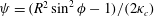 $\unicode[STIX]{x1D713}=(R^{2}\sin ^{2}\unicode[STIX]{x1D719}-1)/(2\unicode[STIX]{x1D705}_{c})$
, which, when substituted into (B 7), returns
$\unicode[STIX]{x1D713}=(R^{2}\sin ^{2}\unicode[STIX]{x1D719}-1)/(2\unicode[STIX]{x1D705}_{c})$
, which, when substituted into (B 7), returns
 $B_{0}=1$
, and so
$B_{0}=1$
, and so
 $$\begin{eqnarray}B(\unicode[STIX]{x1D713})=\sqrt{1+2\unicode[STIX]{x1D705}_{c}\unicode[STIX]{x1D713}}.\end{eqnarray}$$
It may be helpful to clarify that the previous inlet streamfunction is evaluated here at the top of the cone, namely, at the wall where
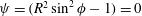 $\unicode[STIX]{x1D713}=(R^{2}\sin ^{2}\unicode[STIX]{x1D719}-1)=0$
and where
$\unicode[STIX]{x1D713}=(R^{2}\sin ^{2}\unicode[STIX]{x1D719}-1)=0$
and where
 $B=1$
. Next, we may update (B 8) into
$B=1$
. Next, we may update (B 8) into
 $$\begin{eqnarray}u_{\unicode[STIX]{x1D703}}=\frac{1}{R\sin \unicode[STIX]{x1D719}}\sqrt{1+2\unicode[STIX]{x1D705}_{c}\unicode[STIX]{x1D713}}.\end{eqnarray}$$
Note that we recover (3.8) along the inlet section, where a uniform flow prevails. Finally, using the streamfunction inside the cone, we retrieve (3.17).
B.3 Spherical to cylindrical transformation
In order to obtain (3.19), our expressions are switched from spherical to polar cylindrical coordinates using the standard transformation matrix,
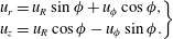 $$\begin{eqnarray}\left.\begin{array}{@{}c@{}}\displaystyle u_{r}=u_{R}\sin \unicode[STIX]{x1D719}+u_{\unicode[STIX]{x1D719}}\cos \unicode[STIX]{x1D719},\\ \displaystyle u_{z}=u_{R}\cos \unicode[STIX]{x1D719}-u_{\unicode[STIX]{x1D719}}\sin \unicode[STIX]{x1D719}.\end{array}\right\}\end{eqnarray}$$


 Open access