


1. Introduction
The realization of long-term storage of CO2 in deep saline aquifers (Metz, Davidson & De Coninck Reference Metz, Davidson and De Coninck2005; Basbug & Gumrah Reference Basbug and Gumrah2009; Michael et al. Reference Michael, Arnot, Cook, Ennis-King, Funnell, Kaldi, Kirste and Paterson2009; Orr Reference Orr2009; Pamukcu & Gumrah Reference Pamukcu and Gumrah2009; Huppert & Neufeld Reference Huppert and Neufeld2014), the provision of large-scale thermal-energy storage systems (Singh, Saini & Saini Reference Singh, Saini and Saini2010; Heyde & Schmitz Reference Heyde and Schmitz2017) and the increase in the efficiency of geothermal energy extraction (Ghoreishi-Madiseh et al. Reference Ghoreishi-Madiseh, Hassani, Mohammadian and Radziszewski2013; Böttcher et al. Reference Böttcher, Watanabe, Görke and Kolditz2016) are examples of emerging engineering technologies that have the potential to slow down climate change. Natural convection in porous media is a fundamental process relevant to these applications (Hewitt, Neufeld & Lister Reference Hewitt, Neufeld and Lister2012; Liang et al. Reference Liang, Wen, Hesse and DiCarlo2018; Wen et al. Reference Wen, Ahkbari, Zhang and Hesse2018a; Hewitt Reference Hewitt2020; Liu et al. Reference Liu, Jiang, Chong, Zhu, Wan, Verzicco, Stevens, Lohse and Sun2020a). In general, it describes the flow of fluid in a saturated porous medium between two infinite horizontal plates driven by a temperature or species concentration difference. The variation of temperature or species concentration results in the variation of the density, which induces the buoyancy force.
In this paper, we focus on the natural convection in porous media driven by a species concentration gradient. Compared with convective heat transfer, convective mass transfer is usually characterized by high Schmidt numbers  $(Sc)$ and, unlike thermal energy, the mass cannot penetrate the surfaces of solid obstacles. In the absence of a porous medium, the natural convective fluid flow is governed by the dimensionless Rayleigh number, which describes the buoyancy-to-diffusion ratio (Kunes Reference Kunes2012). In the presence of a porous medium, a Rayleigh–Darcy number (hereafter Rayleigh number,
  $Ra$) is introduced; it is a modification of the conventional Rayleigh number, which takes the effect of the porous matrix into account (Nield Reference Nield1994). Mass transfer in natural convection is characterized by the Sherwood number
  $(Sh)$, which is the ratio of the total mass transfer rate (by convection and mass diffusion) to the diffusive mass transfer rate. The onset of natural convection occurs when
  $Sh$ exceeds unity;
  $Sh$ quantifies the efficiency of the mass transfer enhancement due to natural convection.
Besides field research studies (Arts et al. Reference Arts, Chadwick, Eiken, Thibeau and Nooner2008) and laboratory experiments (Kneafsey & Pruess Reference Kneafsey and Pruess2010; Faisal et al. Reference Faisal, Chevalier, Bernabe, Juanes and Sassi2015), numerical simulation is another established tool for understanding convection in porous media. Two approaches are available for the simulation of convection in porous media: pore-scale-resolving direct numerical simulations (DNS) and macroscopic (volume-averaged) simulations. Macroscopic simulations are widely employed in modelling convection in porous media (Nield & Bejan Reference Nield and Bejan2017), due to their significantly lower computational costs. The first macroscopic model for fluid flow in porous media was proposed by Darcy (Reference Darcy1856). Whitaker (Reference Whitaker1969) proposed the most commonly used macroscopic equations for the conservation of volume-averaged quantities. Using Whitaker's approach, the Darcy–Oberbeck–Boussinesq (DOB) equations can be derived, as shown in Nield & Bejan (Reference Nield and Bejan2017). This set of equations has often been used in recent studies; see Hewitt et al. (Reference Hewitt, Neufeld and Lister2012), Hewitt, Neufeld & Lister (Reference Hewitt, Neufeld and Lister2013, Reference Hewitt, Neufeld and Lister2014), Wen, Corson & Chini (Reference Wen, Corson and Chini2015), De Paoli Zonta & Soldati (Reference De Paoli, Zonta and Soldati2016) and Pirozzoli et al. (Reference Pirozzoli, De Paoli, Zonta and Soldati2021) as examples.
A deficiency of the DOB equations is the underlying assumption that convection in porous media is uniquely determined by the Rayleigh number, in which the pore scale is combined with the macroscopic length scale. This simplification could, however, be at the root of reported discrepancies between numerical simulations and experiments. For example, most numerical studies based on the DOB equations indicate a linear scaling of  $Sh$ versus
  $Ra$ in the ultimate regime
  $(Ra \ge 5000)$, whereas the experiments by Neufeld et al. (Reference Neufeld, Hesse, Riaz, Hallworth, Techelepi and Huppert2010) and Keene & Goldstein (Reference Keene and Goldstein2015) exhibited a nonlinear scaling. The experiments by Backhaus, Turitsyn & Ecke (Reference Backhaus, Turitsyn and Ecke2011) in a Hele-Shaw cell, where the flow obeys the Darcy law but there is no porous matrix, also exhibited a nonlinear scaling. However, recent studies showed that nonlinear scaling observed in Hele-Shaw experiments may be related to the three-dimensionality of the flow (Letelier, Mujica & Ortega Reference Letelier, Mujica and Ortega2019; De Paoli, Alipour & Soldati Reference De Paoli, Alipour and Soldati2020). In a recent study of three-dimensional DOB simulation, Pirozzoli et al. (Reference Pirozzoli, De Paoli, Zonta and Soldati2021) indicated that the nonlinear scaling can occur in three-dimensional flows at very high Rayleigh numbers. This could be related to supercells at the boundary, which are the footprint of mega-plumes dominating the interior part of the flow.
Another possible reason for the nonlinear scaling is related to non-Darcy effects induced by the porous matrix. Various studies have been performed to analyse non-Darcy effects in natural convection in porous media. For example, Shao et al. (Reference Shao, Fahs, Younes and Makradi2016) and Wang & Tan (Reference Wang and Tan2009) included the Brinkman term (which is a Laplacian term that is included to model the effect of macroscopic velocity gradients on the momentum transport) in their simulations of convection at low  $Ra$ numbers
  $(Ra \le 5000)$. However, the study of Vasseur, Wang & Sen (Reference Vasseur, Wang and Sen1989) concluded that the Brinkman term is significant only for large Darcy numbers. Mijic, Laforce & Muggeridge (Reference Mijic, Laforce and Muggeridge2014) and Das et al. (Reference Das, Biswal, Roy and Basak2016) included the Forchheimer term in their models to account for the effect of turbulence. In recent years, increasing attention has been paid to hydrodynamic dispersion in porous media; see Hidalgo & Carrera (Reference Hidalgo and Carrera2009), Ghesmat, Hassanzadeh & Abedi (Reference Ghesmat, Hassanzadeh and Abedi2011), Yang & Vafai (Reference Yang and Vafai2011), MacMinn et al. (Reference MacMinn, Neufeld, Hesse and Huppert2012), Wang et al. (Reference Wang, Nakanishi, Hyodo and Suekane2016), Liang et al. (Reference Liang, Wen, Hesse and DiCarlo2018), Wen, Chang & Hesse (Reference Wen, Chang and Hesse2018b), Fahs et al. (Reference Fahs, Graf, Tran, Ataie-Ashtiani, Simmons and Younes2020), Jouybari, Lundström & Hellström (Reference Jouybari, Lundström and Hellström2020) and Liu et al. (Reference Liu, Zhang, Zhao, Jiang and Song2020b). It is sometimes also referred to as thermal dispersion for heat transfer problems (Pedras & de Lemos Reference Pedras and de Lemos2008), or mass dispersion for mass transfer problems (Mesquita & de Lemos Reference Mesquita and De Lemos2004). A Fickian dispersion tensor introduced by Bear (Reference Bear1961) is often used to model the hydrodynamic dispersion. These studies show that hydrodynamic dispersion can have significant effects on convection in porous media, at least for high-Darcy-number problems. Gelhar, Welty & Rehfeldt (Reference Gelhar, Welty and Rehfeldt1992), Neuman (Reference Neuman1990) and Liang et al. (Reference Liang, Wen, Hesse and DiCarlo2018) indicated that the hydrodynamic dispersion is also important at low Darcy numbers, since dispersion at the macroscale (macrodispersivity) is dependent on the scale of the system, rather than the grain size. In a recent study, however, Zech et al. (Reference Zech, Attinger, Bellin, Cvetkovic, Dietrich, Fiori, Teutsch and Dagan2019) showed that dispersion at the macroscale varied widely and did not show any clear effect on the scale of solute plumes.
In the DNS, the Navier–Stokes equations coupled to a convection–diffusion equation for the species concentration (or temperature for heat transfer) are solved, whereby the smallest scale of the porous matrix is resolved. Owing to the high computational costs, this approach has so far only been used for simple geometries of porous matrices (Minkowycz et al. Reference Minkowycz, Sparrow, Schneider and Pletcher2006; Torabi et al. Reference Torabi, Karimi, Peterson and Yee2017). Although DNS is too expensive for engineering applications, it is a powerful tool to gain a better understanding of the physics of convection in porous media and serves as a foundation for developing macroscopic models. Recently, we performed pore-scale-resolving DNS of natural convection in porous media composed of a simple porous matrix (Gasow et al. Reference Gasow, Lin, Zhang, Kuznetsov, Avila and Jin2020). Our DNS results showed that the boundary layer thickness for convection in porous media is determined by the pore size instead of the Rayleigh number. This is distinctly different from classical DOB simulations (Huppert & Neufeld Reference Huppert and Neufeld2014). We also showed that the scaling for the Sherwood number depends on the porosity and the pore-scale parameters and observed that the scaling law becomes nonlinear for porous media with sufficiently high porosity. Furthermore, the computed flow patterns exhibited motions with large length scales, close to the size of the whole domain, which were not found in DOB simulations. In another recent numerical study, Liu et al. (Reference Liu, Jiang, Chong, Zhu, Wan, Verzicco, Stevens, Lohse and Sun2020a) observed that the Nusselt number increases with a decrease in the porosity, while the Rayleigh–Darcy number is kept constant. This trend cannot be captured by the DOB equations. Liu et al. (Reference Liu, Jiang, Chong, Zhu, Wan, Verzicco, Stevens, Lohse and Sun2020a) also indicated that the ratio of the pore scale to the thickness of the thermal boundary layer has a significant effect on the scaling of the Nusselt number versus  $Ra$. A scaling crossover occurs when the thickness of the thermal boundary is comparable to the pore scale. Therefore, the discrepancy between the DOB solutions and the experiments could arise due to pore-scale effects.
In this paper, we develop a new macroscopic model for natural convection in porous media, which accounts for pore-scale effects. Our model is based on a detailed analysis of the DNS simulations of Gasow et al. (Reference Gasow, Lin, Zhang, Kuznetsov, Avila and Jin2020) and additional DNS carried out here. The model involves a coefficient that depends solely on the pore-scale geometry. This coefficient must be determined a priori. For each pore-scale geometry, this coefficient is determined with a single DNS performed with a fixed set of parameters. Subsequently, we show that the simulations of the model agree with our DNS results (e.g. results with respect to the Sherwood number, mean species concentration, root-mean-square (r.m.s.) species concentration and velocity) in wide ranges of pore size, Rayleigh, Schmidt and Darcy numbers.
2. Governing equations and numerical methods
We consider natural convection in a porous medium domain bounded by two walls (figure 1), which is the porous equivalent to the classical Raleigh–Bénard cell (Hewitt Reference Hewitt2020). The computational domain is two-dimensional, and it has a width-to-height ratio  $L/H = 2$. Two different geometries of the generic porous matrix are studied. They are composed of aligned (figure 1b) or staggered (figure 1c) square obstacles. The analysis in this study is mainly based on the results of the first porous matrix, while the sensitivity of our model coefficient to the pore-scale geometry is examined with the second porous matrix. In both cases, the periodically arranged square obstacles with the size d are a distance s apart in the horizontal and vertical directions. The geometry of a representative elementary volume (REV) of the simulated porous medium is a square with a side length s, containing one obstacle.

Figure 1. Structure of the computational domain occupied by a regular porous matrix, with a magnified view of a single REV, used for the DNS (a). A constant species concentration difference at the top and bottom walls and periodic boundary conditions in the horizontal direction are utilized. The porous matrix inside the domain is composed of aligned (b) or staggered square obstacles (c).
Constant species concentrations,  ${c_1}$ and
  ${c_0}$, are maintained at the upper and lower walls of the domain, respectively. The difference of the species concentrations at the upper and lower walls leads to density differences, which drive natural convection in the domain. The horizontal boundary conditions are periodic, whereas the no-slip boundary condition is used at the upper and lower walls and on the surfaces of the obstacles. And because mass cannot penetrate the solid matrix of the porous medium, no mass transfer is assumed at the interface, hence homogeneous Neumann boundary conditions are used at the obstacles for the species concentration. Similar set-ups have been adopted in other numerical studies of convection in porous media; see Javaheri, Abedi & Hassanzadeh (Reference Javaheri, Abedi and Hassanzadeh2010), Hewitt et al. (Reference Hewitt, Neufeld and Lister2012), Wen et al. (Reference Wen, Ahkbari, Zhang and Hesse2018b), and Hewitt (Reference Hewitt2020) as examples.
2.1. Governing equations for DNS
DNS studies were performed to gain insights into the physics of natural convection in the porous medium, to determine the coefficients for the macroscopic model, as well as to obtain the validation data. The governing equations for DNS of natural convection in porous media are the Navier–Stokes equations and the species transport equation. In the flow field, the local species concentration differences are small; hence, the Boussinesq approximation is used to account for the buoyancy force (Herwig Reference Herwig2013). Using Einstein's summation convention, the governing microscopic equations for natural convection in porous media are as follows:
 \begin{gather}\frac{{\partial {u_i}}}{{\partial {x_i}}} = 0,\end{gather}
 \begin{gather}\frac{{\partial {u_i}}}{{\partial t}} + \frac{{\partial ({u_i}{u_j})}}{{\partial {x_j}}} ={-} \frac{{\partial p}}{{\partial {x_i}}} + \nu \frac{{{\partial ^2}{u_i}}}{{\partial x_j^2}} + \beta {g_i}(c - c_{0}),\end{gather}
 \begin{gather}\frac{{\partial c}}{{\partial t}} + \frac{{\partial ({u_i}c)}}{{\partial {x_i}}} = {D_f}\frac{{{\partial ^2}c}}{{\partial x_j^2}},\end{gather}
where  $\nu $,
  ${D_f}$,
  ${u_i}$, p,
  ${g_i}$ and c are the kinematic viscosity, the mass diffusivity, the ith component of the velocity vector, the pressure, the ith component of the gravity vector and the species concentration, respectively. The concentration expansion coefficient is defined as
  $\beta = \beta ({c_0}) ={-} (1/{\rho _0}){(\partial \rho /\partial c)_{{c_0}}}$ (see Herwig & Moschallski, Reference Herwig and Moschallski2009), where
  $\rho $ is the fluid density.
The Sherwood number  $Sh$ is calculated from the DNS as the ratio of the total mass transfer rate
  $\dot{m}$ (by convection and diffusion) to the mass transfer rate
  ${\dot{m}_{diff}}$ (by diffusion only) across the lower or upper wall (Baehr & Stephan Reference Baehr and Stephan2006):
 \begin{equation}Sh =
\frac{{\dot{m}}}{{{{\dot{m}}_{diff}}}} = \frac{{\displaystyle\int_w
{\overline {\frac{{\partial c}}{{\partial {x_2}}}}
\,\textrm{d}A} }}{{\displaystyle\int_w {{{\left. {\overline
{\frac{{\partial c}}{{\partial {x_2}}}} } \right|}_{R{a_f}
= 0}}\,}
\textrm{d}A}},\end{equation}
\begin{equation}Sh =
\frac{{\dot{m}}}{{{{\dot{m}}_{diff}}}} = \frac{{\displaystyle\int_w
{\overline {\frac{{\partial c}}{{\partial {x_2}}}}
\,\textrm{d}A} }}{{\displaystyle\int_w {{{\left. {\overline
{\frac{{\partial c}}{{\partial {x_2}}}} } \right|}_{R{a_f}
= 0}}\,}
\textrm{d}A}},\end{equation}where the bar denotes the time-averaging operator, while the subscript w denotes either the upper or lower wall surface.
2.2. Macroscopic equations
The macroscopic equations are obtained by averaging the Navier–Stokes equations and the species transport equations (2.1)–(2.3) over each REV (see figure 1). This method of averaging is similar to that used in de Lemos (Reference De Lemos2012); however, de Lemos (Reference De Lemos2012) carried out a time and volume averaging over each respective REV, while we performed only volume averaging. The macroscopic equations read:
 \begin{gather}\frac{\partial \overset{\lower0.5em\hbox{$\smash{\scriptscriptstyle\smile}$}}{u}_{i}}{{\partial {\overset{\lower0.5em\hbox{$\smash{\scriptscriptstyle\smile}$}}{x}_i}}} = 0,\end{gather}
 \begin{gather}\frac{{\partial {\overset{\lower0.5em\hbox{$\smash{\scriptscriptstyle\smile}$}}{u}_i}}}{{\partial \overset{\lower0.5em\hbox{$\smash{\scriptscriptstyle\smile}$}}{t} }} + \frac{{\partial ({\overset{\lower0.5em\hbox{$\smash{\scriptscriptstyle\smile}$}}{u}_i}{\overset{\lower0.5em\hbox{$\smash{\scriptscriptstyle\smile}$}}{u}_i}/\phi )}}{{\partial {\overset{\lower0.5em\hbox{$\smash{\scriptscriptstyle\smile}$}}{x}_j}}} + \frac{{\partial (\phi {{{\langle ^i}{u_i}{}^i{u_j}\rangle }^i})}}{{\partial {\overset{\lower0.5em\hbox{$\smash{\scriptscriptstyle\smile}$}}{x}_j}}} ={-} \frac{{\partial (\phi {{\langle p\rangle }^i})}}{{\partial {\overset{\lower0.5em\hbox{$\smash{\scriptscriptstyle\smile}$}}{x}_i}}} + \nu \frac{{{\partial ^2}{\overset{\lower0.5em\hbox{$\smash{\scriptscriptstyle\smile}$}}{u}_i}}}{{\partial \overset{\lower0.5em\hbox{$\smash{\scriptscriptstyle\smile}$}}{x} _j^2}} - \phi \beta {g_i}(\overset{\lower0.5em\hbox{$\smash{\scriptscriptstyle\smile}$}}{c} - {c_0}) - \phi {\overset{\lower0.5em\hbox{$\smash{\scriptscriptstyle\smile}$}}{R} _i},\end{gather}
 \begin{gather}\frac{{\partial (\phi \overset{\lower0.5em\hbox{$\smash{\scriptscriptstyle\smile}$}}{c} )}}{{\partial \overset{\lower0.5em\hbox{$\smash{\scriptscriptstyle\smile}$}}{t} }} + \frac{{\partial ({\overset{\lower0.5em\hbox{$\smash{\scriptscriptstyle\smile}$}}{u}_i}\overset{\lower0.5em\hbox{$\smash{\scriptscriptstyle\smile}$}}{c} )}}{{\partial {\overset{\lower0.5em\hbox{$\smash{\scriptscriptstyle\smile}$}}{x}_i}}} + \frac{{\partial (\phi {{\langle {}^i{u_i}{}^ic\rangle }^i})}}{{\partial {\overset{\lower0.5em\hbox{$\smash{\scriptscriptstyle\smile}$}}{x}_j}}} = {D_m}\frac{{{\partial ^2}\overset{\lower0.5em\hbox{$\smash{\scriptscriptstyle\smile}$}}{c} }}{{\partial \overset{\lower0.5em\hbox{$\smash{\scriptscriptstyle\smile}$}}{x} _j^2}},\end{gather}
where the sign  $\overset{\lower0.5em\hbox{$\smash{\scriptscriptstyle\smile}$}}{ }$ denotes an REV-averaged quantity. The operator
  ${\langle \;\;\rangle ^i}$ denotes the intrinsic volume averaging in the fluid phase, which is adopted from Whitaker (Reference Whitaker1986). The left superscript i denotes the intrinsic deviation of a volume-averaged quantity, e.g.
  ${}^i{u_i} = {u_i} - {\langle \; {u_i}\rangle ^i}$. The porosity
  $\phi $ is defined as
  $\phi = {V_{void\ space}}/{V_{total}}$,
  ${\overset{\lower0.5em\hbox{$\smash{\scriptscriptstyle\smile}$}}{u} _i} = \phi {\langle {u_i}\rangle ^i}$ is the volume-averaged velocity, which is often referred to as the superficial velocity, and
  $\overset{\lower0.5em\hbox{$\smash{\scriptscriptstyle\smile}$}}{c} = {\langle c\rangle ^i}$ is the intrinsic averaged mass concentration. The subscript m denotes an effective property in the volume-averaged equations, e.g.
  ${D_m}$ is the effective mass diffusivity. Simulations of small domains are needed to determine the value of
  ${D_m}$ for a specific pore-scale geometry (see Gasow et al. Reference Gasow, Lin, Zhang, Kuznetsov, Avila and Jin2020).
The terms  $\phi {\langle {}^i{u_i}{}^i{u_j}\rangle ^i}$,
  $\phi {\langle {}^i{u_i}{}^ic\rangle ^i}$ and
  ${\overset{\lower0.5em\hbox{$\smash{\scriptscriptstyle\smile}$}}{R} _i}$ are the momentum dispersion, mass dispersion and total drag, respectively. The momentum and mass dispersion terms have been neglected in our model due to the underlying assumptions for convection in porous media with low Darcy numbers (see Appendix A1). Since the local Reynolds number
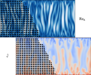
  $R{e_K} = \left|\boldsymbol{\overset{\lower0.5em\hbox{$\smash{\scriptscriptstyle\smile}$}}{u}} \right|\sqrt K /\nu$ in our simulations is generally smaller than unity (Gasow et al. Reference Gasow, Lin, Zhang, Kuznetsov, Avila and Jin2020), the Forchheimer term in
  ${\overset{\lower0.5em\hbox{$\smash{\scriptscriptstyle\smile}$}}{R} _i}$ can also be neglected (Nield & Bejan Reference Nield and Bejan2017). The effects of the macroscopic velocity gradient on
  ${\overset{\lower0.5em\hbox{$\smash{\scriptscriptstyle\smile}$}}{R} _i}$ can be modelled with a Laplacian term, which was first proposed by Brinkman (Reference Brinkman1949) and then was extensively studied and improved; see Rao, Kuznetsov & Jin (Reference Rao, Kuznetsov and Jin2020), Zaripov, Mardanov & Sharafutdinov (Reference Zaripov, Mardanov and Sharafutdinov2019), Zhao et al. (Reference Zhao, Wang, Li, Zhang and Mahabaleshwar2018), Liu, Patil & Narusawa (Reference Liu, Patil and Narusawa2007), Valdes-Parada, Ochoa-Tapia & Alvarez-Ramirez (Reference Valdes-Parada, Ochoa-Tapia and Alvarez-Ramirez2007), Vafai (Reference Vafai2005), Starov & Zhdanov (Reference Starov and Zhdanov2001) and Ochoa-Tapia & Whitaker (Reference Ochoa-Tapia and Whitaker1995) as examples. Here, we model the sum of the total drag
  ${\overset{\lower0.5em\hbox{$\smash{\scriptscriptstyle\smile}$}}{R} _i}$ and the diffusion term
  $\nu ({\partial ^2}{\overset{\lower0.5em\hbox{$\smash{\scriptscriptstyle\smile}$}}{u} _i}/\partial \overset{\lower0.5em\hbox{$\smash{\scriptscriptstyle\smile}$}}{x} _j^2)$ in (2.6) as
 \begin{equation}\nu \frac{{{\partial ^2}{\overset{\lower0.5em\hbox{$\smash{\scriptscriptstyle\smile}$}}{u}_i}}}{{\partial \overset{\lower0.5em\hbox{$\smash{\scriptscriptstyle\smile}$}}{x} _j^2}} + {\overset{\lower0.5em\hbox{$\smash{\scriptscriptstyle\smile}$}}{R} _i} = \frac{\nu }{K}{\overset{\lower0.5em\hbox{$\smash{\scriptscriptstyle\smile}$}}{u} _i} + {\nu _m}\frac{{{\partial ^2}{\overset{\lower0.5em\hbox{$\smash{\scriptscriptstyle\smile}$}}{u}_i}}}{{\partial \overset{\lower0.5em\hbox{$\smash{\scriptscriptstyle\smile}$}}{x} _j^2}},\end{equation}
where K and  ${\nu _m}$ are the permeability and effective viscosity of the porous medium. Simulations of small domains are needed to determine their values a priori (see Gasow et al. (Reference Gasow, Lin, Zhang, Kuznetsov, Avila and Jin2020) for details of how they were determined). The macroscopic momentum equation (2.6) is hence simplified to
 \begin{equation}\frac{{\partial {\overset{\lower0.5em\hbox{$\smash{\scriptscriptstyle\smile}$}}{u}_i}}}{{\partial \overset{\lower0.5em\hbox{$\smash{\scriptscriptstyle\smile}$}}{t} }} + \frac{{\partial ({\overset{\lower0.5em\hbox{$\smash{\scriptscriptstyle\smile}$}}{u}_i}{\overset{\lower0.5em\hbox{$\smash{\scriptscriptstyle\smile}$}}{u}_i}/\phi )}}{{\partial {\overset{\lower0.5em\hbox{$\smash{\scriptscriptstyle\smile}$}}{x}_j}}} ={-} \frac{{\partial (\phi {{\langle p\rangle }^i})}}{{\partial {\overset{\lower0.5em\hbox{$\smash{\scriptscriptstyle\smile}$}}{x}_i}}} + {\nu _m}\frac{{{\partial ^2}{\overset{\lower0.5em\hbox{$\smash{\scriptscriptstyle\smile}$}}{u}_i}}}{{\partial \overset{\lower0.5em\hbox{$\smash{\scriptscriptstyle\smile}$}}{x} _j^2}} - \phi \beta {g_i}(\overset{\lower0.5em\hbox{$\smash{\scriptscriptstyle\smile}$}}{c} - {c_0}) - \phi \frac{\nu }{K}{\overset{\lower0.5em\hbox{$\smash{\scriptscriptstyle\smile}$}}{u} _i}.\end{equation}
2.3. Two-length-scale diffusion assumption
Normalizing the governing equations (2.5), (2.9) and (2.7) using the characteristic concentration difference  $\Delta c = {c_1} - {c_0}$, velocity
  ${u_m} = \beta \Delta cgK/\nu $, length
  $H$ and time
  ${t_m} = H/{u_m}$, the following dimensionless macroscopic equations are obtained:
 \begin{gather}\frac{{\partial {{\hat{u}}_i}}}{{\partial {{\hat{x}}_i}}} = 0,\end{gather}
 \begin{gather}\frac{{\partial {{\hat{u}}_i}}}{{\partial \hat{t}}} + \frac{{\partial ({{\hat{u}}_i}{{\hat{u}}_i}/\phi )}}{{\partial {{\hat{x}}_j}}} ={-} \frac{{\partial (\phi {{\langle \tilde{p}\rangle }^i})}}{{\partial {{\hat{x}}_i}}} + \frac{{{a_\nu }Sc}}{{{\gamma _m}Ra}}\frac{{{\partial ^2}{{\hat{u}}_i}}}{{\partial \hat{x}_j^2}} - \frac{{\phi \textrm{Sc}}}{{{\gamma _m}RaDa}}{z_i}\hat{c} - \frac{{\phi Sc}}{{{\gamma _m}RaDa}}{\hat{u}_i},\end{gather}
 \begin{gather}\frac{{\partial (\phi \hat{c})}}{{\partial \hat{t}}} + \frac{{\partial ({{\hat{u}}_i}\hat{c})}}{{\partial {{\hat{x}}_i}}} = \frac{1}{{Ra}}\frac{{{\partial ^2}\hat{c}}}{{\partial \hat{x}_j^2}}.\end{gather}
Here  $\hat {}$ denotes a dimensionless volume-averaged quantity,
  $\hat{c}$ is the dimensionless volume-averaged species concentration defined as
  $\hat{c} = ({\langle c\rangle ^i} - {c_0})/({c_1} - {c_0})$,
  ${a_\nu } = {\nu _m}/\nu $ is the ratio of the effective viscosity
  ${\nu _m}$ to the molecular viscosity of the fluid
  $\nu $, and
  ${\gamma _m} = {D_m}/{D_f}$ is the ratio of the effective mass diffusivity
  ${D_m}$ to the mass diffusivity of the fluid
  ${D_f}$.
The Rayleigh number in (2.11) and (2.12) is defined by using the common definition of this parameter for natural convection in porous media, as in Nield (Reference Nield1994):
 \begin{equation}Ra \equiv \frac{{R{a_f}Da}}{{{\gamma _m}}} = \frac{{H\beta \Delta cgK}}{{{D_m}\nu }}.\end{equation}
The Schmidt number is defined as
 \begin{equation}Sc = \frac{\nu }{{{D_f}}}.\end{equation}
The Darcy number is defined as
 \begin{equation}Da = \frac{K}{{{H^2}}}.\end{equation}
By assuming that  ${a_\nu }$ is independent of
  $Da$ and taking the leading-order terms with respect to
  $1/Da$ in (2.11), one obtains the well-known DOB equations. However, we reported in our recent DNS study (Gasow et al. Reference Gasow, Lin, Zhang, Kuznetsov, Avila and Jin2020) that the boundary layer thickness is determined by the pore size, which is characterized by
  $\sqrt K $. In addition, similar profiles for temporally and horizontally averaged quantities are observed when the distance from the wall is normalized with the pore size. Therefore, the Laplacian term
  $({a_\nu }Sc/{\gamma _m}Ra)({\partial ^2}{\hat{u}_i}/\partial \hat{x}_j^2)$ in (2.11) is expected to scale as
  $1/K$ and should be of order
  $1/Da$, exactly as the Darcy term
  $- (\phi Sc/{\gamma _m}RaDa){\hat{u}_i}$ and the buoyancy force term
 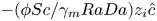 $- (\phi Sc/{\gamma _m}RaDa){z_i}\hat{c}$. Hence, the Laplacian term in the macroscopic equation cannot be neglected even if the Darcy number is small.
We here propose a model for the effective viscosity  ${\nu _m}$ based on a two-length-scale diffusion (TLSD) hypothesis, in which the macroscopic diffusion is determined by the pore size, characterized by
  $\sqrt K $, and the distance between the lower and upper boundaries H. Our TLSD hypothesis is supported by our recent DNS (Gasow et al. Reference Gasow, Lin, Zhang, Kuznetsov, Avila and Jin2020), where we showed that natural convection in porous media is determined by these two length scales. The pore size characterizes the boundary layer thickness and the size of proto-plumes, whereas the distance between the two walls determines the size of mega-plumes.
Based on the TLSD assumption stated above,  ${a_\nu }$ is modelled as
 \begin{equation}{a_\nu } = \frac{{{\nu _m}}}{\nu } = \frac{{a_\nu ^\ast }}{{Da}},\end{equation}
where  $a_\nu ^\ast $ is a constant assumed to be solely determined by the pore-scale geometry of the porous matrix. Note that the two length scales
  $\sqrt K $ and H are combined in
  $Da$. At the upper and lower walls, we imposed constant species concentrations,
  ${c_1}$ and
  ${c_0}$, respectively, and the no-slip boundary condition.
It should be noted that only the leading-order terms of  $Da$ for diffusion are kept in the macroscopic equations (2.10)–(2.12). As
  $Da \to 0$, the macroscopic governing equations can be further simplified to
 \begin{gather}\frac{{\partial {{\hat{u}}_i}}}{{\partial {{\hat{x}}_i}}} = 0,\end{gather}
 \begin{gather}\frac{{\partial \hat{p}}}{{\partial {{\hat{x}}_i}}} + \hat{c}{z_i} + {\hat{u}_i} = \frac{{a_\nu ^\ast }}{\phi }\frac{{{\partial ^2}{{\hat{u}}_i}}}{{\partial \hat{x}_j^2}},\end{gather}
 \begin{gather}\frac{{\partial \hat{c}}}{{\partial \hat{t}^*}} + \frac{{\partial ({{\hat{u}}_i}\hat{c})}}{{\partial {{\hat{x}}_i}}} = \frac{1}{{Ra}}\frac{{{\partial ^2}\hat{c}}}{{\partial \hat{x}_j^2}},\end{gather}
where 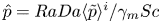 $\hat{p} = RaDa{\langle \tilde{p}\rangle ^i}/{\gamma _m}Sc$ is the normalized pressure. The dimensionless time is modified to be
  $\hat{t}^* = \overset{\lower0.5em\hbox{$\smash{\scriptscriptstyle\smile}$}}{t} /\phi $. These macroscopic equations (2.17)–(2.19) become the DOB equations if
  $a_\nu ^\ast $ is set to zero. When the DOB equations are solved, only the velocity component in the wall-normal direction is set to zero at the upper and lower walls. This boundary condition was also used in other DOB simulations; see Hewitt et al. (Reference Hewitt, Neufeld and Lister2014) and Wen et al. (Reference Wen, Corson and Chini2015) as examples. In this paper, the macroscopic simulations were carried out by solving equations (2.10)–(2.12), so that the effect of the Darcy number can be assessed. The Sherwood number for the macroscopic model simulations is defined using the same definition as for the DNS, which is given in (2.4).
2.4. Numerical method
For the simulations, a finite-volume method (FVM) was utilized. The solvers were developed by using the open-source code package OpenFoam 6. The spatial discretization was implemented by a second-order central-difference scheme. For time derivatives, the second-order implicit backward method was used. For the correction and coupling of the pressure and velocity fields, the pressure-implicit scheme with splitting of operators (PISO) algorithm was used (Versteeg & Malalasekera Reference Versteeg and Malalasekera2007). A stabilized preconditioned (bi)conjugate gradient solver was utilized to solve the pressure field and the momentum and species concentration equations. We have performed the code validation for our DNS solver extensively in our previous studies (Jin et al. Reference Jin, Uth, Kuznetsov and Herwig2015; Uth et al. Reference Uth, Jin, Kuznetsov and Herwig2016; Jin & Kuznetsov Reference Jin and Kuznetsov2017; Gasow et al. Reference Gasow, Lin, Zhang, Kuznetsov, Avila and Jin2020).
3. Studied test cases
3.1. Description of the test cases
We continued selected DNS cases of Gasow et al. (Reference Gasow, Lin, Zhang, Kuznetsov, Avila and Jin2020) to improve the statistics and thus to allow a more thorough validation of our hypothesis. In addition, we also computed these cases by solving the macroscopic equations (2.10)–(2.12) with our two-length-scale diffusion model. The Rayleigh numbers  $Ra$ are up to
  $20\;000$ and the Schmidt numbers
  $Sc$ are
  $1$ and
  $250$. The ranges of geometrical parameters of the studied test cases are given in table 1. For both DNS and macroscopic simulation cases
  ${u_i} = 0$ and
  $c = ({c_1} - {c_0})/2$ were used as initial conditions.
Table 1. Ranges of geometrical parameters for the studied test cases.

To obtain representative statistical results, the time averaging, denoted by the bar over, of the respective variable was performed after the flow and mass concentration fields reached a statistically steady state. As an example, the time evolutions of the instantaneous Sherwood number for the DNS case with  $H/s = 100$,
  $s/d = 1.5$,
  $Ra = 20\;000$ and
  $Sc = 250$ are shown in figure 2. The time averaging of the Sherwood number has been started after the time marked by the red dashed line. At least 200 dimensionless time units
  $H/{u_m}$ are calculated to obtain the statistical results.

Figure 2. The time evolution of the instantaneous Sherwood number for the DNS case with  $H/s = 50$,
  $s/d = 1.5$,
  $Ra = 20\;000$ and
  $Sc = 250$. The dashed red line marks the time at which the time averaging is started; and
  $\hat{t} = t{u_m}/H$ is the dimensionless time.
3.2. Determination of the model coefficient
The coefficient  $a_\nu ^\ast $ for a specific pore-scale geometry cannot be computed a priori with simulations of small domains (as for the other model parameters). Here, we empirically determine
  $a_\nu ^\ast $ by simulating natural convection within the specific pore-scale geometry with fixed values of
  $H/s$,
  $Sc$ and
  $Ra$. Since we only keep the leading-order terms of the order
  $Da$ in our model equations, a test case with a sufficiently small Darcy number should be used to ensure that the higher-order terms of Da are negligible. In particular, we performed a parametric study for
  $a_\nu ^\ast (\phi )$ while keeping
  $H/s = 20,\;Sc = 250$ and
  $Ra = 20\;000$ fixed. These parameter values were selected because the Sherwood number from DNS marginally changes as
  $H/s$ is increased (i.e. as the pore size is decreased); hence the effect of higher-order terms of Da on Sh can be safely neglected. The value of
  $a_\nu ^\ast $ is selected for each considered porosity value, so that the Sherwood number from the macroscopic simulation matches the DNS results. Figure 3 shows the dependence of
  $a_\nu ^\ast $ on the porosity
  $\phi $.

Figure 3. Dependence of the model coefficient  $a_\nu ^\ast $ on the porosity
  $\phi $, for porous matrices composed of aligned and staggered square obstacles.
We expect that  $a_\nu ^\ast $ is a geometrical parameter that is independent of
  $Sc$,
$Sc$,  $Ra$ and Da. This will be examined later in § 5. The value of
  $a_\nu ^\ast $ only mildly changes when the porous matrix is switched from aligned squares to staggered squares. According to our DNS results,
  $a_\nu ^\ast $ can be well correlated by
 \begin{equation}a_v^\ast (\phi ) = 7.5 \times {10^{ - 5}}{\phi ^9}.\end{equation}
This correlation has reasonable accuracy for  $0.28 < \phi < 0.95$. However, the variations of pore-scale geometries used in this study are limited. In particular, the flow structures in randomly packed porous matrices may be distinctly different from those in regularly packed porous matrices (Liu et al. Reference Liu, Jiang, Chong, Zhu, Wan, Verzicco, Stevens, Lohse and Sun2020a). Studies with more pore-scale geometries are needed to test the generality of (3.1).
3.3. Mesh and time-step independence studies
The mesh and time-step independence studies for the DNS cases have already been performed in our previous work (see Gasow et al. Reference Gasow, Lin, Zhang, Kuznetsov, Avila and Jin2020). Here we focus on the influence of the mesh and time step on the macroscopic simulation results (solution of (2.10)–(2.12)). The numerical results for the Sherwood number are shown in table 2. At least 200 dimensionless time units  $H/{u_m}$ were calculated to obtain the statistical results.
Table 2. Influence of mesh and time step on the Sherwood number  $Sh$. The test case with
  $H/s = 50$,
  $s/d = 1.5$,
  $Ra = 20\;000$ and
  $Sc = 250$ is used in the parametric study. The cases c, d, e and f are considered to be mesh- and time-step-independent. The mesh resolution and maximum Courant number of the case f (in italic) are used in all cases of macroscopic simulation.

The results of the resolution study show that the Sherwood number is under predicted if the mesh resolution is too low (see table 2 cases a and b) or the maximum Courant number is too high (see table 2 case g). According to the mesh/time-step independence study,  $C{o_{max}} = 0.8$ and mesh resolution 2000×3200 (case f) were used for all cases of macroscopic simulation. The numerical error of
  $Sh$ in the macroscopic simulations is estimated to be 2.8 %, which is the maximum variation of
  $Sh$ in the cases c, d, e and f. All simulations were performed on the clusters of the HLRN (North-German Supercomputing Alliance), using 2× Intel Cascade Lake Platinum 9242 CPUs (CLX-AP) with 96 cores per node. The DNS cases use up to
  $7.2 \times {10^7}$ mesh cells, which requires a parallel computing time of 1200 hours using 384 processors. The macroscopic simulation cases use up to
  $6.4 \times {10^6}$ mesh cells.
4. DNS results
In this section, we focus on an a priori verification of the TLSD hypothesis. The model results are compared with the DNS results in § 5.
4.1. Budget of the macroscopic kinetic energy
The budget for the time- and line-averaged macroscopic kinetic energy  ${\langle \bar{K}\rangle ^{x1}} = {\textstyle{1 \over 2}}{\langle \overset{\lower0.5em\hbox{$\smash{\scriptscriptstyle\smile}$}}{u} _i^2\rangle ^{x1}}$ was calculated from the DNS for
  $Ra = 20\;000,\;s/d = 1.5$,
  $s/d = 1.25$,
  $Sc = 250$ and
  $Da$ in the range
  $3.5 \times {10^{ - 7}}\textrm{ to }3.5 \times {10^{ - 5}}$. By averaging the momentum equation (2.2) over REVs, taking the dot product with the superficial velocity
  ${\overset{\lower0.5em\hbox{$\smash{\scriptscriptstyle\smile}$}}{u} _i} = \phi {\langle {u_i}\rangle ^i}$, and then averaging in time and in the horizontal direction
  ${x_1}$, we obtained the following equation for
  ${\langle \bar{K}\rangle ^{x1}}$:
 \begin{align}&- {\left\langle
\overline {{\overset{\lower0.5em\hbox{$\smash{\scriptscriptstyle\smile}$}}{u}_i}\phi {{\left\langle {\frac{{\partial
({u_i}{u_j})}}{{\partial {x_j}}}} \right\rangle }^i}}
\right\rangle^{x1}} - {\left\langle
\overline {{\overset{\lower0.5em\hbox{$\smash{\scriptscriptstyle\smile}$}}{u}_i}\phi {{\left\langle {\frac{{\partial
p}}{{\partial {x_i}}}} \right\rangle }^i}} \right\rangle^{x1}} + {\left\langle \overline {{\overset{\lower0.5em\hbox{$\smash{\scriptscriptstyle\smile}$}}{u}_i}\phi
{{\left\langle {\nu \frac{{{\partial^2}{u_i}}}{{\partial
x_j^2}}} \right\rangle }^i}}\right\rangle ^{x1}}\notag\\
&\quad + {\langle \overline {{\overset{\lower0.5em\hbox{$\smash{\scriptscriptstyle\smile}$}}{u}_i}\phi {{\langle
\beta {g_i}(c - {c_0})\rangle }^i}}\rangle^{x1}} =
0.\end{align}
\begin{align}&- {\left\langle
\overline {{\overset{\lower0.5em\hbox{$\smash{\scriptscriptstyle\smile}$}}{u}_i}\phi {{\left\langle {\frac{{\partial
({u_i}{u_j})}}{{\partial {x_j}}}} \right\rangle }^i}}
\right\rangle^{x1}} - {\left\langle
\overline {{\overset{\lower0.5em\hbox{$\smash{\scriptscriptstyle\smile}$}}{u}_i}\phi {{\left\langle {\frac{{\partial
p}}{{\partial {x_i}}}} \right\rangle }^i}} \right\rangle^{x1}} + {\left\langle \overline {{\overset{\lower0.5em\hbox{$\smash{\scriptscriptstyle\smile}$}}{u}_i}\phi
{{\left\langle {\nu \frac{{{\partial^2}{u_i}}}{{\partial
x_j^2}}} \right\rangle }^i}}\right\rangle ^{x1}}\notag\\
&\quad + {\langle \overline {{\overset{\lower0.5em\hbox{$\smash{\scriptscriptstyle\smile}$}}{u}_i}\phi {{\langle
\beta {g_i}(c - {c_0})\rangle }^i}}\rangle^{x1}} =
0.\end{align}
Equation (4.1) shows that the budget for  ${\langle \bar{K}\rangle ^{x1}}$ includes:
• the production by the buoyancy force,
 ${K_{buoy}} = {\langle \overline {{\overset{\lower0.5em\hbox{$\smash{\scriptscriptstyle\smile}$}}{u}_i}\phi {{\langle \beta {g_i}(c - {c_0})\rangle }^i}}\rangle^{x1}}$;
• the loss due to viscous dissipation,
${K_{diff}} = {\langle \overline {{\overset{\lower0.5em\hbox{$\smash{\scriptscriptstyle\smile}$}}{u}_i}\phi {{\langle \nu ({\partial ^2}{u_i}/\partial x_j^2)\rangle }^i}}\rangle^{x1}}$;• the loss due to pressure gradient,
${K_{pres}} ={-} {\langle \overline {{\overset{\lower0.5em\hbox{$\smash{\scriptscriptstyle\smile}$}}{u}_i}\phi {{\langle \partial p/\partial {x_i}\rangle }^i}}\rangle^{x1}}$;• the transport due to convection,
${K_{conv}} ={-} {\langle \overline {{\overset{\lower0.5em\hbox{$\smash{\scriptscriptstyle\smile}$}}{u}_i}\phi {{\langle \partial ({u_i}{u_j})/\partial {x_j}\rangle }^i}}\rangle^{x1}}$.
In the DOB equations, the Darcy term (Darcy drag) is the only source of losses of macroscopic kinetic energy. The Darcy losses read
 \begin{equation}{K_{Darcy}} ={-} \phi (\nu /K){\langle \overline {\overset{\lower0.5em\hbox{$\smash{\scriptscriptstyle\smile}$}}{u}_i^2}\rangle^{x1}}.\end{equation}
The budget of  ${\langle \bar{K}\rangle ^{x1}}$ is studied using the test case with
  $s/d = 1.5\ (\phi = 0.56)$,
  $H/s = 20$,
  $Ra = 20\;000$,
  $Da = 8.8 \times {10^{ - 6}}$ and
  $Sc = 250$. Figure 4 shows the distribution of
  ${K_{buoy}}$,
  ${K_{diff}}$,
  ${K_{pres}}$ and
  ${K_{conv}}$ in the wall-normal direction. They are normalized with the characteristic kinetic energy
  ${K_{mean}} = {\textstyle{1 \over 2}}\; u_m^2$ or
  ${K_{buoy}}$. The distance from the lower wall is normalized with the pore size s. It is evident that more macroscopic kinetic energy is produced by the buoyancy force in the central region than in the region close to the wall. The transport of
  ${\langle \bar{K}\rangle ^{x1}}$ due to convection is much smaller than
  ${K_{buoy}}$, so it can be neglected. Here
  $- {K_{diff}}$ and
  $- {K_{pres}}$ are the losses of the macroscopic kinetic energy. Both
  $- {K_{diff}}$ and
  $- {K_{pres}}$ increase with increasing distance from the wall
  ${x_2}/s$. The loss of
  ${\langle \bar{K}\rangle ^{x1}}$ in the region close to the wall is mainly due to the pressure gradient
  $- {K_{pres}}$.

Figure 4. Distribution of the budget of the macroscopic kinetic energy  ${\langle \bar{K}\rangle ^{x1}}$ in the wall-normal direction. Here
  $s/d = 1.5\ (\phi = 0.56)$,
  $H/s = 20\ (Da = 8.8 \times {10^{ - 6}})$,
  $Ra = 20\;000$ and
  $Sc = 250$.
Figure 5 shows the loss of the macroscopic kinetic energy due to the Darcy drag  ${K_{Darcy}}$ (assuming that the superficial velocity calculated from the macroscopic simulation is identical to the DNS solution). The drag
  ${K_{Darcy}}$ is normalized by
  ${K_{mean}}$ or
  ${K_{buoy}}$. It can be seen that
  ${K_{Darcy}}$ is close to
  ${K_{buoy}}$ in the region away from the wall
  $({x_2}/s \gg 0)$. However,
  ${K_{Darcy}}/{K_{buoy}}$ is smaller than 0.85 in the first three REVs adjacent to the wall
  $({x_2}/s < 3)$. The DNS results confirm that the Darcy term, which accounts for the losses due to the Darcy drag, cannot account for all the losses of the macroscopic kinetic energy.

Figure 5. Distribution of the loss of the macroscopic kinetic energy  ${\langle \bar{K}\rangle ^{x1}}$ due to the Darcy drag. Here
  $s/d = 1.5\ (\phi = 0.56)$,
  $H/s = 20\ (Da = 8.8 \times {10^{ - 6}})$,
  $Ra = 20\;000$ and
  $Sc = 250$.
The question arises of whether the difference between  ${K_{Darcy}}$ and
  ${K_{buoy}}$ shown in figure 5 is because the Darcy number in the DNS case is not small enough. To answer this question,
  ${K_{pres}}/{K_{buoy}}$,
  ${K_{diff}}/{K_{buoy}}$,
  ${K_{conv}}/{K_{buoy}}$ and
  ${K_{darcy}}/{K_{buoy}}$ in the first REV cell next to the bottom wall for different Darcy numbers are compared in figure 6. It is evident from this figure that all of these quantities stay almost constant as the Darcy number is decreased from
  $3.5 \times {10^{ - 5}}$ to
  $3.5 \times {10^{ - 7}}$, suggesting that the Darcy numbers in our DNS cases are small enough for the presented analysis. The Darcy number has a noticeable effect as it is increased to
  ${\sim} 3 \times {10^{ - 5}}$. In this case,
  ${K_{pres}}/{K_{buoy}}$ and
  ${K_{Darcy}}/{K_{buoy}}$ become smaller,
  ${K_{diff}}/{K_{buoy}}$ becomes larger, whereas
  ${K_{conv}}/{K_{buoy}}$ is still negligibly small. We speculate that higher
  ${K_{diff}}$ at very large Darcy numbers is due to the mass dispersion, which is neglected in our macroscopic model (convection with very large Darcy numbers is out of the scope of this study).

Figure 6. Plots of  ${K_{pres}}/{K_{buoy}}$ (a),
  ${K_{diff}}/{K_{buoy}}$ (b),
  ${K_{conv}}/{K_{buoy}}$(c) and
  ${K_{Darcy}}/{K_{buoy}}$ (d) in the first REV cell next to the bottom wall versus the Darcy number. Here
  $s/d = 1.5\ (\phi = 0.56)$ with
  $H/s = 10,\;20,\;50,\;100$ and
  $s/d = 1.25\ (\phi = 0.36)$ with
  $H/s = 10,\;20,\;50$,
  $Ra = 20\;000$ and
  $Sc = 250$.
Our budget analysis shows that, in the near-wall region, there is a difference between the loss due to the Darcy drag  ${K_{Darcy}}$ and the overall loss, which is identical to
  $- {K_{buoy}}$. Since the transport of
  ${\langle \bar{K}\rangle ^{x1}}$ is negligibly small, this suggests that another source for the loss of
  ${\langle \bar{K}\rangle ^{x1}}$ should be considered in the macroscopic equations.
4.2. Sh–Da dependence
According to our hypothesis, the macroscopic diffusion, the Darcy drag and the buoyancy force are of the same order with respect to the Darcy number, so the macroscopic diffusion cannot be neglected even if the Darcy number is small. To examine our hypothesis, we investigated the relationship between the Sherwood number and the Darcy number. We varied  $Da$ in the range
  $3.5 \times {10^{ - 7}}\textrm{ to }3.5 \times {10^{ - 5}}$ for
  $s/d = 1.5\ (\phi = 0.56)$ and
  $2.8 \times {10^{ - 7}}\textrm{ to }7 \times {10^{ - 6}}$ for
  $s/d = 1.25\ (\phi = 0.36)$; the corresponding
  $H/s$ ratios are in the range 10–100. If our hypothesis were true, the Sherwood number should gradually become independent of
  $Da$ and should not approach the DOB solution.
The DNS results shown in figure 7 generally support our assumption, i.e. the values of  $Sh$ for
  $Sc = 250$ depend only weakly on
  $Da,$ when
  $Da$ is small enough. The values of
  $Sh$ are also different from the DOB solution. As shown in figure 7(a), the same trend is found for
  $s/d = 1.25\ (\phi = 0.36)$ and
  $Sc = 1$, where
  $Sh$ depends weakly on
  $Da$. The only exception is the case for
  $s/d = 1.5\ (\phi = 0.56)$ and
  $Sc = 1$, where
  $Sh$ still increases with decreasing Da (but it is still far away from the DOB result). Test cases with even smaller Darcy numbers could be computed to probe the Da dependence more thoroughly. However, the calculation of these cases would be extremely expensive and hence out of the scope of this study.

Figure 7. The  $Sh(Da)$ dependence for the DNS and DOB cases. Here
  $s/d = 1.5\ (\phi = 0.56)$ with
  $H/s = 10,\;20,\;50,\;100$ and
  $s/d = 1.25\ (\phi = 0.36)$ with
  $H/s = 10,\;20,\;50$ and
  $Ra = 20\;000$, for (a)
  $Sc = 1$ and (b)
  $Sc = 250$.
It should be noted that the Darcy numbers for real applications are much smaller than the values used in the DNS cases. However, since our DNS results for the Sherwood number are approximately  $Da$-independent, we expect that it is possible to predict the Sherwood numbers using DNS with relatively higher (computationally affordable) Darcy numbers.
In a recent DNS study, Liu et al. (Reference Liu, Jiang, Chong, Zhu, Wan, Verzicco, Stevens, Lohse and Sun2020a) proposed the following correlation for estimating the Nusselt number (equivalent to  $Sh$ in this study):
 \begin{equation}Sh \approx c{\kern 1pt} \phi {\left( {\frac{H}{l}} \right)^4}S{c^2}Re_{rms}^2Ra_f^{ - 1} + 1,\end{equation}
where c is an undetermined constant according to the work of Grossmann & Lohse (Reference Grossmann and Lohse2000, Reference Grossmann and Lohse2001, Reference Grossmann and Lohse2004),  $\; l$ is the minimum spacing between the obstacles,
  $R{e_{rms}} = {U_{rms}}l/\nu $ is the Reynolds number based on the volume-averaged r.m.s. velocity magnitude, and
  $R{a_f} = {H^3}\beta \Delta cg/\nu {D_f}$ is the Rayleigh number defined for the free fluid flow. If we set the value of c to
  $1250$ and determine
  ${U_{rms}}$ from our DNS results, the results of (4.3) are in good agreement with our DNS results for different values of
  $\phi $ and
  $Sc$ (see figure 8). It should be noted that (4.3) is proposed based on the flow condition that viscosity dominates; hence intense kinetic energy dissipation takes place within the bulk domain and turbulence is suppressed in the pore canals. For the volume- and time-averaged kinetic energy dissipation rate
  ${\langle {\epsilon _u}\rangle ^{v,t}}$, the following proportionality is valid:
  ${\langle {\epsilon _u}\rangle ^{v,t}}\sim \phi \nu U_{rms}^2/{l^2}$. This corresponds to the ∞ regime of classical Rayleigh–Bénard convection (without porous media) introduced by Grossmann & Lohse (Reference Grossmann and Lohse2001) for large
  $Sc$ and small
  $R{a_f}$. A good agreement between predictions obtained using (4.3) and our DNS results indicates the significance of macroscopic diffusion in momentum transport.

Figure 8. Sherwood number versus the Rayleigh number for  $Ra$ in the range
  $500 - 20\;000$ compared to the correlation proposed by Liu et al. (Reference Liu, Jiang, Chong, Zhu, Wan, Verzicco, Stevens, Lohse and Sun2020a), with (a)
  $Sc = 1$ and (b)
  $Sc = 250$.
5. Macroscopic modelling results
Since the leading-order terms of  $Da$ for diffusion are accounted for in the TLSD model, this model can be used in principle to calculate cases characterized by small Darcy numbers. In this section, we test whether and how the model results approach the DNS results as
  $Da \to 0$. In addition, we investigate the range of parameters for the validity of the TLSD model.
5.1. Sherwood number
Figure 9 shows the relationship between the Sherwood number and the Rayleigh number when  $H/s$ is 20 and Rayleigh numbers are up to
  $20\;000$. The results of our macroscopic model are compared with the correlation obtained from the DNS results (see Gasow et al. Reference Gasow, Lin, Zhang, Kuznetsov, Avila and Jin2020) as well as the DOB results. In the DNS,
  $Sh$ depends on
  $s/d$ or
  $\phi $ for
  $Ra > 2000$. The value of
  $Sh$ increases as
  $s/d$ or
  $\phi $ decreases, while the difference becomes larger as
  $Ra$ increases. In the large-Rayleigh-number regime
  $(Ra \ge 5000)$, the
  $Sh = f(Ra)$ scaling changes from a linear scaling
  $Sh\sim Ra$ for
  $s/d = 1.25$
  $(\phi = 0.36)$ to a nonlinear scaling
  $Sh\sim R{a^{0.8}}$ for
  $s/d = 1.5$
  $(\phi = 0.56)$, see figure 9(a). These characteristics are not captured in DOB simulations but are well reproduced in our macroscopic model simulations.

Figure 9. Sherwood number versus the Rayleigh number with  $Ra$ in the range
  $500 - 20\;000$ and
  $H/s = 20$ for three values of the Darcy number:
  $Da = 8.8 \times {10^{ - 6}}\ (s/d = 1.5)$,
  $Da = 5.4 \times {10^{ - 6}}\ (s/d = 1.4)$ and
  $Da = 1.8 \times {10^{ - 6}}\ (s/d = 1.25)$, with (a)
  $Sc = 1$ and (b)
  $Sc = 250$.
For the current small  $H/s$ (or
  $Da$) value, both DNS and model results show that the Sherwood number increases as the Schmidt number is increased from 1 to 250. Similar to
  $Sc = 1$, the scaling for
  $Sc = 250$ also changes from linear
  $(Sh\sim Ra)$ for
  $s/d = 1.25$
  $(\phi = 0.36)$ to nonlinear
  $(Sh\sim R{a^{0.8}})$ for
  $s/d = 1.5\ (\phi = 0.56)$. This behaviour is reproduced in our macroscopic model solution, whereas the effect of the Schmidt number is not accounted for in the DOB equations.
We neglected the high-order terms with respect to  $Da$ when we proposed the TLSD model. However, since the leading-order term with respect to
  $Da$ is kept in the momentum equation (2.11), the effect of
  $Da$ on natural convection can still be accounted for when its value is small enough. The relationship between the Sherwood number and the Darcy number for
  $Ra = 20\;000$,
  $Sc = 1$ or 250, and
  $s/d = 1.5$ or 1.25 (
 $\phi = 0.56$ or 0.36) is shown in figure 10. The macroscopic model results are compared with the DNS results as well as with the DOB results. Recall that
  $a_\nu ^\ast $ is only related to the pore-scale geometry and is independent of the flow conditions and the Darcy number. The macroscopic model simulations are in good agreement with the DNS for
  $Da \le 2 \times {10^{ - 6}}$ and for different Schmidt numbers. By contrast, the DOB results are independent of the Darcy and Schmidt numbers. The DOB simulations overpredict the Sherwood number for
  $s/d = 1.5\ (\phi = 0.56)$ and underpredict Sh for
  $s/d = 1.25\ (\phi = 0.36)$.

Figure 10. Sherwood number versus the Darcy number for  $s/d = 1.5\ (\phi = 0.56)$ with
  $H/s = 10,\;20,\;50,\;100$ and
  $s/d = 1.25\ (\phi = 0.36)$ with
  $H/s = 10,\;20,\;50$,
  $Ra = 20\;000$, for (a)
  $Sc = 1$ and (b)
  $Sc = 250$.
5.2. Species concentration and velocity statistics
The vertical profiles of the temporally and horizontally averaged macroscopic quantities (time- and line-averaged species concentration  ${\langle \overline {\hat{c}} \rangle ^{x1}}$, species concentration fluctuation
  ${\langle {\hat{c}^{rms}}\rangle ^{x1}}$, and velocity fluctuations
  ${\langle \hat{u}_1^{rms}\rangle ^{x1}}$ and
  ${\langle \hat{u}_2^{rms}\rangle ^{x1}}$) for
  $s/d = 1.5$ (
 $\phi = 0.56$) and
  $Sc = 1$ are shown in figure 11. The Rayleigh numbers are
  $5000\;\textrm{and}\;20\;000$. The results of our macroscopic TLSD model are compared with the DNS results as well as the DOB results. It is evident that our macroscopic TLSD modelling results for
  ${\langle \overline {\hat{c}} \rangle ^{x1}}$,
  ${\langle \hat{u}_1^{rms}\rangle ^{x1}}$ and
  ${\langle \hat{u}_2^{rms}\rangle ^{x1}}$ are more accurate than the DOB results in the first REV next to the wall. The DNS results show that all statistical results can be well scaled by the pore size s and that the influence of the bounding walls is limited to within the first three REVs next to the wall (Gasow et al. Reference Gasow, Lin, Zhang, Kuznetsov, Avila and Jin2020). Thus, the boundary layer thickness is determined by the pore size s, instead of the Rayleigh number, as suggested in Huppert & Neufeld (Reference Huppert and Neufeld2014). These features are all well captured in the macroscopic simulation.

Figure 11. The vertical profiles of the temporally and horizontally averaged macroscopic quantities for  $s/d = 1.5\ (\phi = 0.56)$,
  $H/s = 20\ (Da = 8.8 \times {10^{ - 6}})$ and
  $Sc = 1$. The Rayleigh number
  $Ra$ is varied. The distance from the wall is normalized by the pore size s. (a) Time- and line-averaged species concentration
  ${\langle \overline {\hat{c}} \rangle ^{x1}}$; (b) r.m.s. of the species concentration fluctuation
  ${\langle {\hat{c}^{rms}}\rangle ^{x1}}$; (c) streamwise velocity fluctuation
  ${\langle \hat{u}_1^{rms}\rangle ^{x1}}$; and (d) wall-normal velocity fluctuation
  ${\langle \hat{u}_2^{rms}\rangle ^{x1}}$.
The same statistical quantities are shown in figure 12 for  $Sc = 250$. It can be seen that these statistical quantities are only marginally changed when a much higher Schmidt number is used in the simulation. Similar to the results for
  $Sc = 1$, the macroscopic modelling results are also in good agreement with the DNS results. The macroscopic TLSD model simulation predicts higher mass concentration
  ${\langle \overline {\hat{c}} \rangle ^{x1}}$ in the first REV next to the wall and higher transverse velocity fluctuation
  ${\langle \hat{u}_2^{rms}\rangle ^{x1}}$. One possible reason for this discrepancy is that the neglected high-order terms with respect to
  $Da$ may lead to modelling errors in the boundary layer region. The TLSD model accuracy can be further improved by decomposing the flow domain into a boundary layer region and a central region, so the modelling in the boundary layer region can be improved. However, this would make the model more complicated and difficult to apply. This modelling approach is not adopted in our study to achieve a compromise between the accuracy and simplicity of the macroscopic model.

Figure 12. The vertical profiles of the temporally and horizontally averaged macroscopic quantities for  $s/d = 1.5\ (\phi = 0.56)$,
  $H/s = 20\ (Da = 8.8 \times {10^{ - 6}})$ and
  $Sc = 250$. The Rayleigh number
  $Ra$ is varied. The distance from the wall is normalized by the pore size s. (a) Time- and line-averaged species concentration
  ${\langle \overline {\hat{c}} \rangle ^{x1}}$; (b) r.m.s. of the species concentration fluctuation
 ${\langle {\hat{c}^{rms}}\rangle ^{x1}}$; (c) streamwise velocity fluctuation
  ${\langle \hat{u}_1^{rms}\rangle ^{x1}}$; and (d) wall-normal velocity fluctuation
  ${\langle \hat{u}_2^{rms}\rangle ^{x1}}$.
5.3. Transient macroscopic fields
To validate the results of our macroscopic TLSD model, we first compare the transient flow fields obtained from macroscopic simulations of (2.10)–(2.12) with those obtained from the DNS results discussed in the previous section and the DOB simulations reported in Gasow et al. (Reference Gasow, Lin, Zhang, Kuznetsov, Avila and Jin2020). For this purpose, the velocity field and the species concentration obtained with the macroscopic simulations and the DNS were volume-averaged (over each REV).
The distribution of the instantaneous  $R{e_K} = (|\boldsymbol{u} |{K^{1/2}})/\nu $ for
  $Ra = 20\;000$,
  $s/d = 1.5\ (\phi = 0.56)$,
  $H/s = 100$ and
  $Sc = 250$ is shown in figure 13. The macroscopic TLSD solution (figure 13c) is qualitatively similar to the DNS solution (figure 13a) and DOB solution (figure 13b). Both the DNS solution and macroscopic solutions indicate that the local Reynolds number is
  $R{e_K} < 4 \times {10^{ - 3}}$. This shows that the studied parameter range is well in the Darcy regime
  $(R{e_K} < 1)$, hence the Forchheimer term in the momentum equation can be safely neglected. Despite the laminar flow in the pore scale, the macroscopic flow field is transient and chaotic. However, the strong spatial variation of the velocity field obtained from the DNS is captured neither in TLSD nor in the DOB simulations.

Figure 13. Instantaneous volume-averaged Reynolds number  $R{e_K}$,
  $H/s = 100\ (Da = 3.5 \times {10^{ - 7}})$,
  $s/d = 1.5\ (\phi = 0.56)$,
  $Ra = 20\;000$ and
  $Sc = 250$: (a) DNS, (b) DOB and (c) TLSD.
Snapshots of the instantaneous species concentrations for  $H/s = 100$,
  $s/d = 1.5\ (\phi = 0.56)$,
  $Ra = 20\;000$ and
  $Sc = 250$ are shown in figure 14. The DNS solution (figure 14a), TLSD solution (figure 14c) and the DOB solution (figure 14b) all exhibit large mega-plume structures in the internal region and small proto-plumes in the boundary layers. They occur due to the rising of a fluid with low species concentration and the sinking of a fluid with high species concentration, forming the instabilities in the boundary layer region (Hewitt et al. Reference Hewitt, Neufeld and Lister2012; Kränzien & Jin Reference Kränzien and Jin2019).

Figure 14. Instantaneous volume-averaged species concentration  $\hat{c}$,
  $H/s = 100\ (Da = 3.5 \times {10^{ - 7}})$,
  $s/d = 1.5\ (\phi = 0.56)$,
  $Ra = 20\;000$ and
  $Sc = 250$: (a) DNS, (b) DOB and (c) TLSD.
While the macroscopic TLSD model and DOB solution exhibit relatively regular mega-plumes, in the DNS solution the mega-plumes are more irregular and chaotic. A possible reason is that the Darcy number in our simulation is still not small enough, while the TLSD model is proposed for problems with low Darcy numbers. The transient flow field from macroscopic simulation converges slower than the Sherwood number and other statistical results with decreasing  $Da$.
$Da$.
The DNS study reported in Gasow et al. (Reference Gasow, Lin, Zhang, Kuznetsov, Avila and Jin2020) shows that the number of mega-plumes increases with the decrease of  $Da$. Figure 15 shows the time-averaged fast Fourier transform (FFT) of the dimensionless mass concentration
  $\hat{c}$ along the centreline at
  ${x_2} = H/2$. The peak wavenumber calculated from the TLSD simulation is still higher than the DNS result, but it is lower than the DOB result. Figure 16 shows that the peak wavenumber from DNS approaches the TLSD or DOB results as the Darcy number approaches 0. However, DNS of natural convection with smaller Darcy numbers are still needed to confirm that the peak wavenumber from DNS will not exceed the TLSD results and approach the DOB results.

Figure 15. Average spectra of the dimensionless mass concentration,  $\hat{c}$, of the DNS, DOB and TLSD results at mid-height
  ${x_2} = H/2$,
  $H/s = 100\ (Da = 3.5 \times {10^{ - 7}})$,
  $s/d = 1.5\ (\phi = 0.56)$,
  $Ra = 20\;000$ and
  $Sc = 250$.

Figure 16. Peak wavenumber k for the mega-plumes of the DNS, DOB and TLSD results for different Darcy numbers with  $s/d = 1.5\ (\phi = 0.56)$,
  $Ra = 20\;000$ and
  $Sc = 250$.
The three-dimensional DOB simulations by Pirozzoli et al. (Reference Pirozzoli, De Paoli, Zonta and Soldati2021) revealed the supercells at the boundary, which are the footprints of mega-plumes dominating the interior part of the flow. They suggest that these supercells might lead to the nonlinear scaling of  $Sh(Ra)$ in the ultimate regime of high Ra numbers. Future work needs to investigate whether these supercells will be also captured by three-dimensional TLSD simulations. Elucidating how macroscopic diffusion affects the plume structures is also a subject of future investigation.
6. Conclusions
The DNS results of Gasow et al. (Reference Gasow, Lin, Zhang, Kuznetsov, Avila and Jin2020) (extended in this study) show that the pore-scale geometry also has significant effects on natural convection in porous media, in particular, the boundary layer thickness is determined by the pore size instead of the Rayleigh number. Based on this, we have proposed the following TLSD model: we assume that pore-scale structures affect the momentum transport through macroscopic diffusion. The macroscopic diffusion is of the same order with respect to the Darcy number as the Darcy drag and the buoyancy force; thus, it cannot be neglected even if the Darcy number is small. It is determined by two length scales: the pore size characterized by  $\sqrt K $ and the distance between the lower and upper boundaries H.
The DNS results show that the loss of the macroscopic kinetic energy is mainly due to microscopic diffusion and the pressure gradient. The loss captured in Darcy's law is only part of the overall loss, even if the superficial velocity is accurately calculated in the DOB equation. The macroscopic diffusion term added here to the momentum equation accounts for the additional loss of the macroscopic kinetic energy. Our DNS results also show that the Sherwood number is almost independent of the Darcy number when the Darcy number is small enough. Thus, the diffusion term is of the same order of the Darcy number  $(Da = K/{H^2})$ as the buoyancy force term and the Darcy term.
A new macroscopic model for simulating natural convection in porous media is developed based on the TLSD assumption. The results of our model are validated extensively by comparison with the DNS as well as the DOB results. The comparison shows that the new macroscopic model performs well as long as  $Da \le 2 \times {10^{ - 6}}$. Simulations of the model predict a much more accurate Sherwood number, r.m.s. mass concentration and r.m.s. velocity than simulations that employ the DOB equations. They also predict the structures of mega-plumes and proto-plumes with reasonable accuracy. In particular, the new model results show that the
  $Sh = f(Ra)$ scaling changes from a linear scaling to a nonlinear scaling as the porosity increases. If the Rayleigh number and Darcy number are fixed, the Sherwood number increases with the increase of the Schmidt number and the decrease of the porosity. These trends agree with the DNS results, whereas they cannot be captured by the DOB simulations. We expect that these trends, as well as the TLSD assumption, also apply to three-dimensional flows. However, how macroscopic diffusion affects the plume structures remains an open question.
Some discrepancies between the new macroscopic modelling results and the DNS results can be found in the boundary layer. The new macroscopic model over predicts the mean mass concentration in the first REV next to the wall. This error may be reduced if the higher-order terms with respect to  $Da$, e.g. the mass dispersion, are considered. However, the current macroscopic model appears preferable due to its simplicity.
This work is the first step towards modelling fundamental issues arising at the pore scale in CO2 sequestration processes. However, it should be noted that a real CO2 sequestration process is much more complicated. It has been extensively investigated by numerical modelling in the last two decades (Weir, White & Kissling Reference Weir, White and Kissling1995, Reference Weir, White and Kissling1996; Lindeberg & Wessel-Berg Reference Lindeberg and Wessel-Berg1997; Hassanzadeh, Pooladi-Darvish & Keith Reference Hassanzadeh, Pooladi-Darvish and Keith2005, Reference Hassanzadeh, Pooladi-Darvish and Keith2007; Bickle et al. Reference Bickle, Chadwick, Huppert, Hallworth and Lyle2007; Pruess & Zhang Reference Pruess and Zhang2008; Chen et al. Reference Chen, Harp, Lin, Keating and Pawar2018). It is characterized by three-dimensional, inherently transient multiphase flow with much more complicated pore-scale geometries and much lower Darcy numbers than those studied in this research (Michael et al. Reference Michael, Golab, Shulakova, Ennis-King, Allinson, Sharma and Aiken2010; Riley Reference Riley2010; Huppert & Neufeld Reference Huppert and Neufeld2014).
Funding
The authors gratefully acknowledge the support of this study by the DFG (Deutsche Forschungsgemeinschaft, 408356608) and the HLRN (North-German Supercomputing Alliance). A.V.K. acknowledges with gratitude the support of the National Science Foundation (award CBET-2042834) and the Alexander von Humboldt Foundation through the Humboldt Research Award.
Declaration of interests
The authors report no conflict of interest.
Appendix A. Momentum dispersion and species concentration dispersion
Breugem, Boersma & Uittenbogaard (Reference Breugem, Boersma and Uittenbogaard2006) argued that momentum dispersion has negligible effects on convection in porous media. This agrees with the study by Rao et al. (Reference Rao, Kuznetsov and Jin2020), who showed numerically that momentum dispersion should be accounted for only when the local Reynolds number  $R{e_K} \gg 1$. Hence, the momentum dispersion is neglected here as well.
The effects of mass dispersion (or thermal dispersion for heat transfer problems) have been extensively studied in recent years, as discussed in the Introduction (Liang et al. Reference Liang, Wen, Hesse and DiCarlo2018; Wen et al. Reference Wen, Ahkbari, Zhang and Hesse2018b; Alomar Reference Alomar2019; Fahs et al. Reference Fahs, Graf, Tran, Ataie-Ashtiani, Simmons and Younes2020). The dispersion term in (2.7) is often modelled using a Fickian dispersion tensor, first introduced by Bear (Reference Bear1961) and expressed as
 \begin{equation}\phi {\langle {}^i{u_i}{}^ic\rangle ^i} = {D_{ij}}\frac{{\partial \overset{\lower0.5em\hbox{$\smash{\scriptscriptstyle\smile}$}}{c} }}{{\partial {\overset{\lower0.5em\hbox{$\smash{\scriptscriptstyle\smile}$}}{x}_j}}},\end{equation}
where the dispersion tensor  ${D_{ij}}$ is calculated as
 \begin{equation}{D_{ij}} = ({\alpha _l} - {\alpha _t}){\overset{\lower0.5em\hbox{$\smash{\scriptscriptstyle\smile}$}}{u} _i}{\overset{\lower0.5em\hbox{$\smash{\scriptscriptstyle\smile}$}}{u} _j}/|\boldsymbol{\overset{\lower0.5em\hbox{$\smash{\scriptscriptstyle\smile}$}}{u}}|+ {\alpha _t}{\delta _{ij}}|\boldsymbol{\overset{\lower0.5em\hbox{$\smash{\scriptscriptstyle\smile}$}}{u}}|,\end{equation}
with  ${\alpha _l}$ and
  ${\alpha _t}$ the longitudinal and transverse diffusivities, respectively. They can be determined from the numerical results for the flow and mass transfer in an REV with a linear concentration gradient in the streamwise or transverse direction; see Nakayama & Kuwahara (Reference Nakayama and Kuwahara1999) and Pedras & de Lemos (Reference Pedras and de Lemos2008). These studies suggest that
  ${D_{ij}}$ has a scaling of the form
  ${D_{ij}}\sim Pe_K^n$, where the local Péclet number
  $P{e_K}$ is defined as
 \begin{equation}P{e_K} = R{e_K}Sc = \frac{{|\boldsymbol{\overset{\lower0.5em\hbox{$\smash{\scriptscriptstyle\smile}$}}{u}}|}}{{{u_m}}}R{e_m}D{a^{1/2}},\end{equation}
where  $R{e_K} = |\boldsymbol{\overset{\lower0.5em\hbox{$\smash{\scriptscriptstyle\smile}$}}{u}}|\sqrt K /\nu $ and
  $R{e_m} = {u_m}H/\nu $ are the local and global Reynolds numbers, respectively. Delgado (Reference Delgado2007) and Nakayama & Kuwahara (Reference Nakayama and Kuwahara1999) suggested that the scaling coefficient n is between 1 and 2. As a consequence,
  ${D_{ij}}$ is expected to be of order between
  $D{a^{1/2}}$ and
  $Da$, while
  ${D_m}$ is of order
  $D{a^0}$. When the Darcy number is small enough,
  $|{{D_{ij}}} |\ll {D_m}$. Since we are interested in natural convection with small Darcy numbers, we only retain the leading-order terms with respect to
  $Da$ for diffusion in (2.7). Thus, due to this theoretical derivation, mass dispersion can also be neglected.
The dispersion at the macroscale (macrodispersivity) suggested by Gelhar et al. (Reference Gelhar, Welty and Rehfeldt1992), Lallemand-Barres & Peaudecerf (1978), Neuman (Reference Neuman1990) and Liang et al. (Reference Liang, Wen, Hesse and DiCarlo2018) is not considered in this study since its effect on the plume scale has not yet been fully elucidated (Zech et al. Reference Zech, Attinger, Bellin, Cvetkovic, Dietrich, Fiori, Teutsch and Dagan2019). Instead, the effect of dispersion is modelled as macroscopic diffusion in the momentum equation. The macroscopic diffusion affects the velocity field and then accounts for the dispersion in the species concentration indirectly.


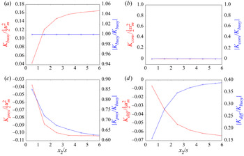


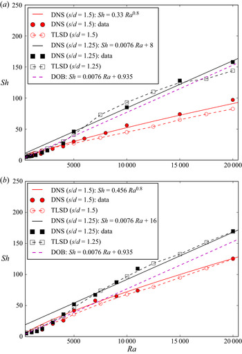


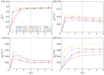


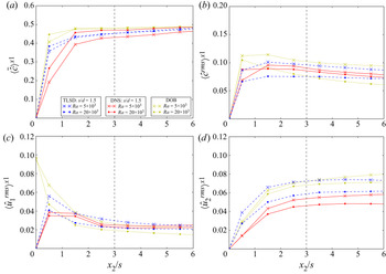


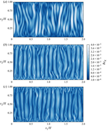


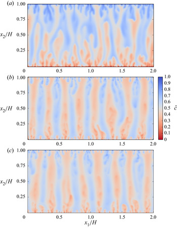


 Open access