


1. Introduction
Pulsating flows in pipe or channel flows are laminar provided that the Reynolds numbers are sufficiently low, as is largely the case for vast parts of the cardiovascular system. In the large arteries, however, blood flow may experience instability, generating large fluctuating shear stresses, which are a possible cause for cardiovascular diseases (Chiu & Chien Reference Chiu and Chien2011). The compliance of arteries plays a major role in blood transport, such as maintaining blood pressure and regularising the flow rate (Ku Reference Ku1997). The flexibility of the aorta is also a key element in minimising pressure fluctuations of blood provided by the left ventricle and distributing oxygen-rich blood through capillaries (O'Rourke & Hashimoto Reference O'Rourke and Hashimoto2007). For these reasons, both flexible walls and pulsatile flow are ubiquitous in the physiological context. When a pulsatile flow interacts with compliant walls, a better analysis of the development of instabilities is therefore required in order to improve our understanding of the link between wall-shear-stress distributions and flow dynamics.
The theory of viscous flow interacting with compliant walls has come a long way from Gray's (Reference Gray1936) initial observations of the outstanding performance of dolphin skins in delaying turbulence, to the recent review of Kumaran (Reference Kumaran2021) enlightening us on the various instability mechanisms. In the 1950s, Kramer conducted pioneering tests in water by towing a dolphin-shaped object covered with viscoelastic materials of varying compliance (Kramer Reference Kramer1957). The author shows that the compliant coating leads to a significant drag reduction and suggests that the dolphin's secret originates in the laminarisation of the flow due to its skin material.
On one hand, several researchers tried and failed to replicate Kramer's experiments; see Gad-el-Hak (Reference Gad-el-Hak1986, Reference Gad-el-Hak1996) for reviews. On the other hand, theoretical results of Carpenter & Garrad (Reference Carpenter and Garrad1985) extend the first analytical studies developed by Benjamin (Reference Benjamin1959, Reference Benjamin1960, Reference Benjamin1963) and Landahl (Reference Landahl1962) and demonstrate that a suitable choice of wall properties could control the onset of the primary instability mode of a flat-plate boundary layer, the so-called Tollmien–Schlichting (TS) mode. However, it is also suggested that the emergence of wall-based instability modes due to fluid–structure interactions (also referenced as flow–structure instabilities, FSI) can limit the potential of laminarisation of the flow (Carpenter & Garrad Reference Carpenter and Garrad1986). The FSI modes can be divided into two categories: the travelling-wave flutter (TWF) modes and the (almost static) divergence (DIV) modes. The onset of the DIV mode only occurs for a certain amount of wall dissipation (see Lebbal, Alizard & Pier (Reference Lebbal, Alizard and Pier2022) for a recent investigation). While the physics of TWF modes is fairly well understood using an analogy with the onset of water waves (Miles Reference Miles1957), scientists are still arguing about the physical mechanism behind the DIV mode (either absolute or convective instabilities with a low phase velocity). The first successful experiment to reproduce Kramer's findings was given by Gaster (Reference Gaster1988).
Several attempts to classify instability modes in the presence of fluid–structure interactions were made since the seminal study of Benjamin (Reference Benjamin1963) for a boundary-layer flow developing on either a wavy boundary or an elastic material with given stiffness, mass and damping. In particular, three types of instability mechanism have been considered: TS modes belong to class A, TWF modes are associated with class B and class C modes correspond to almost steady waves, i.e. the DIV mode (see Davies & Carpenter (Reference Davies and Carpenter1997a,Reference Davies and Carpenterb) for the channel-flow case). Apart from these modes, a transition mode is also found by Sen & Arora (Reference Sen and Arora1988), resulting from the coalescence between a TS mode and a TWF mode. For instance, Davies & Carpenter (Reference Davies and Carpenter1997a) have shown that the transition mode could develop inside a flow between a compliant channel for a sufficiently high level of wall damping. For the same flow case, we have recently shown that, while class B modes are mainly driven by the reduced velocity, which corresponds to the ratio of characteristic wall and advection time scales, the class C mode is influenced by both the Reynolds number and the reduced velocity (Lebbal et al. Reference Lebbal, Alizard and Pier2022).
Independently of studies assessing the optimal properties of wall coating to delay transition to turbulence in wall-bounded flows, the stability of pulsatile flow with respect to viscous shear instability modes has been theoretically addressed since the middle of the 1970s (Davis Reference Davis1976). In comparison with steady flows, pulsatile flows are governed by additional control parameters: the pulsation amplitudes and the pulsating frequency, of which the Womersley number  $Wo$ is a non-dimensional measure (see its definition in (3.6a–c) below). In physiological situations, typical Womersley numbers for large blood vessels are in the range $5$–
$5$– $15$ (Ku Reference Ku1997). Within a Floquet theory framework, von Kerczek (Reference von Kerczek1982) shows that the sinusoidally pulsating flow developing between two flat plates is more stable than the steady plane Poiseuille flow for Womersley numbers in excess of $Wo = 12$. This result was confirmed by direct numerical simulations carried out by Singer, Ferziger & Reed (Reference Singer, Ferziger and Reed1989). Using linear Floquet stability analyses and nonlinear numerical simulations, Pier & Schmid (Reference Pier and Schmid2017) explored a large parameter space for the same flow configuration, confirming and extending the earlier results given by von Kerczek (Reference von Kerczek1982).
On the other hand, several authors (Straatman et al. Reference Straatman, Khayat, Haj-Qasem and Steinman2002; Blennerhassett & Bassom Reference Blennerhassett and Bassom2006) have found that the perturbations may experience a strong increase in kinetic energy during the deceleration phase of the pulsatile base flow. This suggests that transient growth mechanisms and nonlinear effects likely come into play during this part of the pulsation cycle and that the flow could possibly break down to turbulence. Recently, such a scenario has been further supported by non-modal stability analyses, experiments and direct numerical simulations for both pipe and channel flows (Xu et al. Reference Xu, Varshney, Ma, Song, Riedl, Avila and Hof2020b; Pier & Schmid Reference Pier and Schmid2021; Xu, Song & Avila Reference Xu, Song and Avila2021).
In spite of major successes achieved so far in the understanding of the dynamics prevailing for either pulsatile base flows or wall flexibility, only few studies address these two effects in combination. Among of them, Tsigklifis & Lucey (Reference Tsigklifis and Lucey2017) investigated numerically the asymptotic linear stability and transient growth for a pulsatile flow in a compliant channel where both vertical and horizontal displacements are allowed. Using Floquet stability analyses, Tsigklifis & Lucey (Reference Tsigklifis and Lucey2017) show that wall flexibility has a stabilising effect for the Womersley number varying from  $5$ to $50$. The combined effect of wall damping and Womersley number is illustrated by these authors for TS and TWF modes. The authors also found that the tangential motion of the wall could be neglected and that the most dangerous perturbation for the asymptotic regime is always two-dimensional. The non-modal transient growth is shown to be increased by wall compliance. However, the symmetry of the perturbation is not discussed by these authors, and it is therefore not clear whether the sinuous or the varicose TWF modes are investigated. In addition, the DIV mode was not considered by Tsigklifis & Lucey (Reference Tsigklifis and Lucey2017). For a steady channel flow and similar compliant walls, the DIV mode has been characterised by Lebbal et al. (Reference Lebbal, Alizard and Pier2022) and is therefore also expected to occur for the pulsatile flow case.
Finally, the influence of the reduced velocity on TWF modes has not yet been considered when the pulsatile base-flow component comes into play and it is not completely clear if the classification made by Benjamin (Reference Benjamin1963) still holds for the pulsatile flow case.
To provide further understanding of the above points, the present study addresses the linear stability properties of small-amplitude perturbations developing in pulsatile flows through compliant channels. This paper is organised as follows. In § 2, we introduce the coupled fluid–structure system, and the base flow and non-dimensional control parameters are given in § 3. The mathematical formulation of the linear stability problem is presented in § 4. The numerical methods to solve and reduce the generalised eigenvalue problem are explained in § 5. Section 6 is devoted to the results and constitutes the main contribution of the paper: discussion of the spectra, influence of the control parameters and spatio-temporal structure of the eigenmodes. In particular, specific attention will be given to providing critical parameters for the onset of instabilities for the different types of modes (TWF, DIV and TS) and symmetries (sinuous and varicose). In that respect, the extension of the classification made by Benjamin (Reference Benjamin1963) for the steady flow to the pulsatile flow case will be discussed. Finally, in § 7 the conclusions are summarised, an attempt is made to assess the relevance of the critical parameter values in practical contexts, and some prospects for future work are given.
2. Fluid–structure interaction model and interface conditions
In the present study, the analysis is restricted to the two-dimensional case. We introduce the Cartesian coordinate system  $(x,y)$ with unit vectors $({\boldsymbol {e}}_x, {\boldsymbol {e}}_y)$ and consider an incompressible Newtonian fluid with dynamic viscosity $\mu$ and density
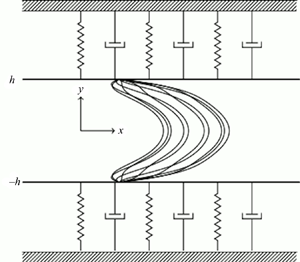
  $\rho$ between two spring-backed deformable plates located at $y =\zeta ^{\pm }(x,t)$ which are allowed to move only in the wall-normal direction (see figure 1). As suggested by previous theoretical analyses carried out by Larose & Grotberg (Reference Larose and Grotberg1997) and Tsigklifis & Lucey (Reference Tsigklifis and Lucey2017) for steady and pulsatile flow cases, respectively, horizontal wall motion only plays a minor role in the dynamics and is therefore not considered in the present investigation for simplicity of the model.

Figure 1. Channel flow with infinite spring-backed flexible walls. (a) Schematic diagram showing the equilibrium state configuration and (b) wall deformation and coordinate system.
The flow between the walls is governed by the incompressible Navier–Stokes equations
 $$\begin{gather} \rho \frac { \partial {\boldsymbol{u}} } { \partial t } + \rho({\boldsymbol{u}}\boldsymbol{\cdot}\boldsymbol{\nabla}){\boldsymbol{u}} ={-}\boldsymbol{\nabla} p + \mu {\rm \Delta} {\boldsymbol{u}}, \end{gather}$$
 $$\begin{gather}0= \boldsymbol{\nabla} \boldsymbol{\cdot} {\boldsymbol{u}}, \end{gather}$$
where  ${\boldsymbol {u}}={u {\boldsymbol {e}}_x+ v {\boldsymbol {e}}_y}$ is the velocity field, with streamwise ( $u$) and wall-normal ( $v$) velocity components and $p$ the pressure field.
The movement of the flexible plates obeys the following equations:
 \begin{equation} m \frac { \partial^2 \zeta^{{\pm}} } { \partial t^2 } +d \frac { \partial \zeta^{{\pm}} } { \partial t } +\left(B\frac{\partial^4}{\partial x^4}-T\frac{\partial^2}{\partial x^2}+K\right)\zeta^{{\pm}} = f^{{\pm}},\end{equation}
where  $m$ denotes the mass per unit area of the plates, $d$ their damping coefficient, $B$ the flexural rigidity, $T$ the wall tension, $K$ the spring stiffness and $f^{\pm }$ represents the $y$-component of the hydrodynamic forces acting on the plates. These forces are obtained as
 \begin{equation} f^{{\pm}}={\boldsymbol{e_y}}\boldsymbol{\cdot} {\boldsymbol{f}}^{{\pm}} \quad\text{with } {\boldsymbol{f}}^{{\pm}}=(\bar{\bar{\tau}}^{{\pm}}-\delta p^{{\pm}}{\boldsymbol{I}}) \boldsymbol{\cdot} {\boldsymbol{n}}^{{\pm}}.\end{equation}
Here,  $\bar {\bar {\tau }}^{\pm }$ denotes the viscous stress tensor at the walls, $\delta p^{\pm }$ the transmural surface pressure and ${\boldsymbol {n}}^{\pm }=(n_x^{\pm },n_y^{\pm })$ is the unit vector normal to the walls pointing towards the fluid. The $y$-component of the normal forces acting on the plate then reads
 \begin{equation} f^{{\pm}}= \mu\left(\left. \frac { \partial u } { \partial y } \right|_{y=\zeta^{{\pm}}}+ \left. \frac { \partial v } { \partial x } \right|_{y=\zeta^{{\pm}}}\right) n_x^{{\pm}} +2\mu\left. \frac { \partial v } { \partial y } \right|_{y=\zeta^{{\pm}}} n_y^{{\pm}} -\delta p^{{\pm}} n_y^{{\pm}},\end{equation}
with
 \begin{equation} n_x^{{\pm}}={\pm} \frac { \partial \zeta^{{\pm}} } { \partial x } \frac{1}{\displaystyle\sqrt{1+ \left( \frac { \partial \zeta^{{\pm}} } { \partial x } \right)^2}} \quad\hbox{and}\quad n_y^{{\pm}}={\mp}\frac{1}{\displaystyle \sqrt{1+ \left( \frac { \partial \zeta^{{\pm}} } { \partial x } \right)^2}}. \end{equation}
Finally, since only vertical displacements are allowed, the no-slip conditions on both walls lead to the kinematic conditions (Wiplier & Ehrenstein Reference Wiplier and Ehrenstein2000)
 \begin{equation} u=0\quad\hbox{and}\quad v= \frac { \partial \zeta^{{\pm}} } { \partial t } \quad\text{for } y=\zeta^{{\pm}}.\end{equation}
The fluid–structure interaction problem is thus fully defined by the coupling of the fluid equations (2.1) and (2.2), the wall equations (2.3) and (2.5) and the boundary conditions (2.7).
3. Base flows and non-dimensional control parameters
A pulsatile base flow, of frequency  $\varOmega$, is considered. Such a flow is driven by a spatially uniform and temporally periodic streamwise pressure gradient and is obtained as an exact solution of the Navier–Stokes equations, assuming a vanishing transmural pressure difference for the unperturbed state. The base-state solution then consists of undeformed parallel walls and of a velocity field in the streamwise direction with profiles that only depend on the wall-normal coordinate and time. It can be expanded as a temporal Fourier series
 \begin{equation} {\boldsymbol{U}}(y,t) = U(y,t){\boldsymbol{e}}_x\quad\text{with } U(y,t)=\sum_{{-\infty<}n{<{+}\infty}} U^{(n)}(y)\exp ({\rm i} n\varOmega t).\end{equation}
Similarly, the pressure gradient that drives the flow is expanded as
 \begin{equation} G(t) = \sum_{{-\infty<}n{<{+}\infty}} G^{(n)}\exp ({\rm i} n\varOmega t),\end{equation}
and is associated with a pulsatile flow rate
 \begin{equation} Q(t)=\sum_{{-\infty<}n{<{+}\infty}} Q^{(n)}\exp ({\rm i} n\varOmega t).\end{equation}
In the above expressions, the conditions  $Q^{(n)} =[Q^{(-n)}]^{\star }, G^{(n)} =[G^{(-n)}]^{\star }$ and $U^{(n)}(y) =[U^{(-n)}(y)]^{\star }$ ensure that all flow quantities are real (with $\star$ denoting complex conjugation). The velocity profile is analytically obtained for each harmonic component. The mean-flow component $U^{(0)}(y)$ corresponds to a parabolic steady Poiseuille flow solution. For $n\neq 0$, the profiles $U^{(n)}(y)$ are obtained in terms of exponential functions (Womersley Reference Womersley1955). Analytical expressions as well as the relationship between $U^{(n)}(y)$ and $Q^{(n)}$ are detailed in the appendix of Pier & Schmid (Reference Pier and Schmid2021). In this work, we focus on pulsatile base flows with a single oscillating component: $-1\leq n \leq 1$ in (3.1)–(3.3). Without loss of generality, $Q^{(1)}$ may then be assumed real, and the flow rate is obtained as
 \begin{equation} Q(t) = Q^{(0)}( 1 + \tilde Q \cos\varOmega t),\end{equation}
with the relative pulsating amplitude  $\tilde Q$ defined as
 \begin{equation} \tilde Q = 2\frac{Q^{(1)}}{Q^{(0)}}.\end{equation}
 The problem is then characterised by  $11$ dimensional parameters: the mean flow rate $[Q^{(0)}] = \rm {m}^{{2}}\ \rm {s}^{-1}$, the half-channel width $[h]=\rm {m}$, the fluid density $[\rho ] = \rm {kg\,m}^{-3}$, the viscosity $[\mu ]=\rm {kg}\ \rm {s}^{-1}\ \rm {m}^{-1}$, the mass of the plate per unit area $[m] = \rm {kg\,m}^{-2}$, the damping coefficient of the wall $[d] = \rm {kg\,m}^{-2}\ \rm {s}^{-1}$, the bending stiffness of the plate $[B] = \rm {kg\,m}^{2}\ \rm {s}^{-2}$, the wall tension $[T]=\rm {kg\,s}^{-2}$, the spring stiffness $[K] = \rm {kg\,m}^{-2}\ \rm {s}^{-2}$, the pulsation frequency $[\varOmega ]=\rm {s}^{-1}$ and the amplitude of the oscillating flow component $[Q^{(1)}]=\rm {m}^{{2}}\ \rm {s}^{-1}$. Hence, the present configuration may be described by eight non-dimensional control parameters.
The base flow is characterised by three non-dimensional parameters
 \begin{equation} Re = \frac{Q^{(0)}}{\nu}, \quad Wo = h\sqrt{\frac{\varOmega}{\nu}} \quad\hbox{and}\quad \tilde Q = 2\frac{Q^{(1)}}{Q^{(0)}}.\end{equation}
Here, the Reynolds number  ${Re}$ is based on the average fluid velocity, the channel diameter and the kinematic viscosity $\nu =\mu /\rho$; the Womersley number ${Wo}$ is a measure of the pulsation frequency and can be interpreted as the ratio of the channel half-diameter $h$ to the thickness $\delta =\sqrt {\nu /\varOmega }$ of the oscillating Stokes boundary layers.
The parameters associated with the walls are non-dimensionalised with respect to the spring stiffness  $K$, which leads to
 \begin{equation} B_*= \frac{B}{K h^4},\quad T_*= \frac{T}{K h^2}\quad\hbox{and}\quad d_*= \frac{d}{\sqrt{m K}}. \end{equation}
Finally, two non-dimensional parameters account for the coupling between the fluid and the compliant walls
 \begin{equation} V_R= \frac{Q^{(0)}}{4h^2}\sqrt{\frac{m}{K}} \quad\hbox{and}\quad \varGamma= \frac{m}{\rho h}.\end{equation}
The reduced velocity  $V_R$ represents the ratio of the wall characteristic time scale $\tau _K=\sqrt {{m}/{K}}$, associated with the spring stiffness, to the characteristic flow advection time scale $\tau _Q={4h^2}/{Q^{(0)}}$ (de Langre Reference de Langre2000). The parameter $\varGamma$ is the mass ratio between the walls and the fluid.
Unperturbed base configurations are thus completely specified by the 8 non-dimensional control parameters (3.6a–c)–(3.8a,b). We further use  $\rho =1, h=1$ and $Q^{(0)}=1$ to uniquely determine dimensional quantities. Hereafter, to reduce the dimensionality of control-parameter space, the mass ratio is kept constant at $\varGamma =2$ and we consider walls without tension $T=0$.
4. Linear stability analysis
For the stability analysis, the total flow fields are decomposed as the superposition of base and small-amplitude perturbation fields
 $$\begin{gather} {\boldsymbol{u}}(x,y,t) = {\boldsymbol{U}}(y,t)+{\boldsymbol{u}}^{\prime}(x,y,t), \end{gather}$$
 $$\begin{gather}p(x,y,t) = G(t)x +p^{\prime}(x,y,t). \end{gather}$$
The wall displacement is similarly written as
 \begin{equation} \zeta^{{\pm}}(x,t)={\pm} h+\eta^{{\pm}\prime}(x,t).\end{equation}
Since the base configuration is homogeneous in  $x$, perturbation fields may be expressed as spatial normal modes
 $$\begin{gather} {\boldsymbol{u}}^\prime(x,y,t) = \tilde{{\boldsymbol{u}}}(y,t){\rm e}^{{\rm i} \alpha x} + {\rm c.c.}, \end{gather}$$
 $$\begin{gather}p^\prime(x,y,t) = \tilde{p}(y,t){\rm e}^{{\rm i} \alpha x} + {\rm c.c.}, \end{gather}$$
 $$\begin{gather}\eta^{{\pm}\prime} (x,t) = \tilde{\eta}^{{\pm}}(t){\rm e}^{{\rm i} \alpha x} + {\rm c.c.}, \end{gather}$$
where  $\alpha$ denotes the streamwise wavenumber and c.c. stands for the complex conjugate. Introducing this decomposition into the governing equations (2.1)–(2.3) and neglecting the quadratic terms leads to the following system of coupled linear partial differential equations:
 $$\begin{gather} \frac { \partial \tilde u } { \partial t } ={-}{\rm i} \alpha U(y,t){\tilde u} - \frac { \partial U } { \partial y } (y,t){\tilde v} -\frac{1}{\rho} {\rm i} \alpha{\tilde p} +\nu\left( \frac { \partial^2 } { \partial y^2 } -\alpha^2\right){\tilde u}, \end{gather}$$
 $$\begin{gather}\frac { \partial \tilde v } { \partial t } ={-}{\rm i} \alpha U(y,t){\tilde v} -\frac{1}{\rho} \frac { \partial {\tilde p} } { \partial y } + \nu\left( \frac { \partial^2 } { \partial y^2 } -\alpha^2\right){\tilde v}, \end{gather}$$
 $$\begin{gather}0 = {\rm i} \alpha{\tilde u}+ \frac { \partial {\tilde v} } { \partial y } , \end{gather}$$
 $$\begin{gather}m \frac { \partial \tilde \gamma^{{\pm}} } { \partial t } ={-} {\rm d} \tilde \gamma^{{\pm}} -(B\alpha^4+T\alpha^2+K){\tilde \eta^{{\pm}}} \pm \tilde p(y,t)|_{{\pm} h} \mp \left.\mu \frac {{\rm d} {\tilde v} } { {\rm d} y } \right|_{{\pm} h}, \end{gather}$$
where we have introduced the additional functions  $\tilde \gamma ^\pm =\partial _t \tilde \eta ^\pm$ in order to reduce the system to first-order differential equations in time. Note that the wall equations (4.10) assume a pressure outside the channel walls always equal to the unperturbed pressure $G(t)x$ prevailing inside (see Lebbal et al. (Reference Lebbal, Alizard and Pier2022) for further details). The same assumption has been made by Davies & Carpenter (Reference Davies and Carpenter1997a,Reference Davies and Carpenterb), Tsigklifis & Lucey (Reference Tsigklifis and Lucey2017) and many others. The effect of the transmural pressure for collapsible channels has been investigated by Luo & Pedley (Reference Luo and Pedley1996) and Xu et al. (Reference Xu, Heil, Seeböck and Avila2020a) and is out the scope of the present study.
The boundary conditions at the perturbed interface are expanded in a Taylor series about their equilibrium values at  $y=\pm h$ (Domaradzki & Metcalfe Reference Domaradzki and Metcalfe1986; Davies & Carpenter Reference Davies and Carpenter1997a; Shankar & Kumaran Reference Shankar and Kumaran2002). At linear order, the flow velocities at the walls are obtained as
 \begin{equation} {\boldsymbol{u}}(x,y=\zeta^{{\pm}},t)={\boldsymbol{u}}^{\prime}(x,y={\pm} h,t) +\left.\eta^{{\pm}\prime}(x,t) \frac {{\rm d} U } { {\rm d} y } \right|_{(y={\pm} h,t)} {\boldsymbol{e_x}}.\end{equation}
Thus, the boundary conditions (2.7) become
 \begin{equation} \left.{\tilde u}(y={\pm} h,t)+\tilde \eta^{{\pm}}(t) \frac {{\rm d} U } { {\rm d} y } \right|_{(y={\pm} h,t)} =0 \quad\hbox{and}\quad {\tilde v}(y={\pm} h,t)=\tilde\gamma^{{\pm}}(t). \end{equation}
Since the base flow is time periodic, the linear stability analysis proceeds by following Floquet theory, where the eigenfunctions are assumed to have the same temporal periodicity as the base flow. The perturbations are therefore further decomposed as
 $$\begin{gather} \tilde{{\boldsymbol{u}}}(y,t) = \left[\sum_{n}{\hat{{\boldsymbol{u}}}^{(n)}(y) \exp{({\rm i} n\varOmega t)}}\right] \exp{(-{\rm i}\omega t)}, \end{gather}$$
 $$\begin{gather}\tilde p(y,t) = \left[\sum_{n}{\hat{p}^{(n)}(y) \exp{({\rm i} n\varOmega t)}}\right] \exp{(-{\rm i}\omega t)}, \end{gather}$$
 $$\begin{gather}\tilde \eta^{{\pm}}(t) = \left[\sum_{n}{\hat{\eta}^{{\pm} (n)}\exp{({\rm i} n\varOmega t)}}\right] \exp{(-{\rm i}\omega t)}, \end{gather}$$
 $$\begin{gather}\tilde \gamma^{{\pm}}(t) = \left[\sum_{n}{\hat{\gamma}^{{\pm} (n)}\exp{({\rm i} n\varOmega t)}}\right] \exp{(-{\rm i}\omega t)}, \end{gather}$$
where the complex frequency  $\omega =\omega _r+{\rm i}\omega _i$ is the eigenvalue, with $\omega _i$ the growth rate and $\omega _r$ the circular frequency. After substitution of these expansions, the linearised equations governing the dynamics of small perturbations take the following form, for each integer $n$:
$n$:
 \begin{align} \omega \hat{u}^{(n)}(y) &= [n\varOmega +i\nu (\partial_{yy} -\alpha^2)] \hat{u}^{(n)}(y) +\frac{\alpha}{\rho} \hat{p}^{(n)}(y) \nonumber\\ &\quad +\sum_{k} \left[ \alpha U^{(k)}(y)\hat{u}^{(n-k)}(y) -i{ \frac {{\rm d} U^{(k)} } { {\rm d} y } \hat{v}^{(n-k)}(y)} \right], \end{align}
 \begin{align} \omega \hat{v}^{(n)}(y) &=[n\varOmega +i \nu (\partial_{yy}-\alpha^2)]\hat{v}^{(n)}(y) +\frac{1}{\rho}\frac{{\rm d} \hat{p}^{(n)}}{{\rm d} y} \nonumber\\ &\quad +\sum_{k} [ \alpha U^{(k)}(y)\hat{v}^{(n-k)}(y) ], \end{align}
 \begin{align} 0&= {\rm i} \alpha\hat{u}^{(n)}(y)+ \frac { \partial \hat{v}^{(n)} } { \partial y } , \end{align}
 \begin{align} \omega\hat{\eta}^{{\pm}(n)} &= n\varOmega \hat\eta^{{\pm}(n)} +i \hat\gamma^{{\pm}(n)}, \end{align}
 \begin{align} \omega\hat{\gamma}^{{\pm}(n)} &= n\varOmega\hat\gamma^{{\pm}(n)} -i\frac{d}{m} \hat{\gamma}^{{\pm}(n)} -\frac{i}{m} (B\alpha^4+T\alpha^2+ K ) \hat{\eta}^{{\pm} (n)} \nonumber\\ &\quad \pm\frac{i}{m} \left(\left.\hat p^{(n)}({\pm} h) -\mu \frac {{\rm d} \hat{v}^{(n)} } { {\rm d} y } \right|_{{\pm} h}\right), \end{align}
together with the kinematic wall conditions
 $$\begin{gather} \hat{u}^{(n)}({\pm} h)= \left. -\sum_{k}{ \frac {{\rm d} U^{(k)} } { {\rm d} y } } \right|_{{\pm} h}\hat{\eta}^{{\pm}(n-k)}, \end{gather}$$
 $$\begin{gather}\hat{v}^{(n)}({\pm} h) =\hat{\gamma}^{{\pm}(n)}. \end{gather}$$
Note that, in (4.17), (4.18) and (4.22), the summation only involves  $-1\leq k \leq +1$ for harmonically pulsating base flows.
The system of coupled linear differential equations (4.17)–(4.21) with boundary conditions (4.22) and (4.23) forms the generalised eigenvalue problem that governs the dynamics of small-amplitude perturbations developing in this time-periodic fluid–structure interaction system.
5. Numerical methods
In this section, we outline the numerical strategy that has been implemented for solving the generalised Floquet eigenvalue problem derived in the previous section. The main objectives in this implementation are the elimination of spurious (non-physical) eigenvalues and the reduction of the required computational effort. To that purpose, we follow the general framework described by Manning, Bamieh & Carlson (Reference Manning, Bamieh and Carlson2007), who have also suggested an interest in the proposed method for handling fluid–structure interaction problems.
The velocity and pressure components are discretised in the wall-normal direction using a Chebyshev collocation method. To suppress spurious pressure modes, we consider the ( $\mathbb {P}_N,\mathbb {P}_{N-2}$)-formulation, where the pressure is approximated with a polynomial of degree $N-2$ while the velocity is discretised with a polynomial of degree $N$ (Schumack, Schultz & Boyd Reference Schumack, Schultz and Boyd1991; Boyd Reference Boyd2001; Peyret Reference Peyret2002). In classical fashion, velocity fields are therefore represented by their values over $N$ Gauss–Lobatto collocation points spanning the entire channel diameter and including the boundary points, while the pressure fields use only the $N-2$ interior points. We note the vectors containing the unknown velocity and pressure components at the interior points for each Fourier mode
 $$\begin{gather} {\boldsymbol{V_I}}^{(n)}= (\hat{u}_2^{(n)}, \ldots, \hat{u}_{N-1}^{(n)}, \hat{v}_2^{(n)}, \ldots, \hat{v}_{N-1}^{(n)} ), \end{gather}$$
 $$\begin{gather}{\boldsymbol{P_I}}^{(n)}= (\hat{p}_2^{(n)}, \ldots, \hat{p}_{N-1}^{(n)}). \end{gather}$$
Similarly, wall displacements and wall velocities are denoted by
 \begin{equation} {\boldsymbol{W}}^{(n)}= (\hat{\eta}_1^{(n)},\hat{\eta}_{N}^{(n)}, \hat{\gamma}_1^{(n)},\hat{\gamma}_{N}^{(n)}).\end{equation}
 The kinematic conditions (4.22) and (4.23) may be used to express the velocity values at the boundaries in terms of the wall variables. As a consequence, the variables  $\hat {u}_1^{(n)}, \hat {v}_1^{(n)}, \hat {u}_{N}^{(n)}$ and $\hat {v}_{N}^{(n)}$ may be directly eliminated from the problem together with the boundary conditions. Then, using
 \begin{equation} \hat{\boldsymbol{X}}^{(n)}=({\boldsymbol{V_I}}^{(n)},{\boldsymbol{P_I}}^{(n)},{\boldsymbol{W}}^{(n)})\end{equation}
for each harmonic of the Floquet eigenvector, the system (4.17)–(4.21) is recast as a generalised algebraic eigenvalue problem of the form
 \begin{equation} \hat{\boldsymbol{A}}^{(n)} \hat{\boldsymbol{X}}^{(n)} +\sum_{k}\hat{\boldsymbol{S}}^{(k)} \hat{\boldsymbol{X}}^{(n-k)} = {\rm i}\omega \hat{\boldsymbol{B}}^{(n)} \hat{\boldsymbol{X}}^{(n)}.\end{equation}
Here, the square matrices  $\hat {\boldsymbol {A}}^{(n)}, \hat {\boldsymbol {S}}^{(k)}$ and $\hat {\boldsymbol {B}}^{(n)}$ are of size $(3N-2)^2$ and may be written in block structure as
 \begin{align} \hat{\boldsymbol{A}}^{(n)} &= \begin{pmatrix} \hat{\boldsymbol{A}}_{\boldsymbol VV}^{(n)} & \hat{\boldsymbol{G}}_{\boldsymbol V} & \hat{\boldsymbol{A}}_{\boldsymbol VW} \\ \hat{\boldsymbol{D}}_{\boldsymbol V} & {\boldsymbol{0}} & \hat{\boldsymbol{D}}_{\boldsymbol W} \\ \hat{\boldsymbol{A}}_{\boldsymbol WV} & \hat{\boldsymbol{G}}_{\boldsymbol W} & \hat{\boldsymbol{A}}_{\boldsymbol WW}^{(n)} \end{pmatrix} ,\quad \hat{\boldsymbol{S}}^{(k)} = \begin{pmatrix} \hat{\boldsymbol{S}}_{\boldsymbol VV}^{(k)} & {\boldsymbol{0}} & \hat{\boldsymbol{S}}_{\boldsymbol VW}^{(k)} \\ {\boldsymbol{0}} & {\boldsymbol{0}} & {\boldsymbol{0}} \\ {\boldsymbol{0}} & {\boldsymbol{0}} & {\boldsymbol{0}} \\ \end{pmatrix} \quad\hbox{and}\notag\\ \hat{\boldsymbol{B}}^{(n)} &= \begin{pmatrix} {\mathbb{I}}_{\boldsymbol VV} & {\boldsymbol{0}} & {\boldsymbol{0}} \\ {\boldsymbol{0}} & {\boldsymbol{0}} & {\boldsymbol{0}} \\ {\boldsymbol{0}} & {\boldsymbol{0}} & {\mathbb{I}}_{\boldsymbol WW} \\ \end{pmatrix}.\end{align}
Their decomposition in terms of square blocks along the diagonal and rectangular blocks off diagonal reflects the structure of the vectors  $\hat {\boldsymbol {X}}^{(n)}$ (5.4), with $2N-4$ variables for ${\boldsymbol {V_I}}^{(n)}, N-2$ variables for ${\boldsymbol {P_I}}^{(n)}$ and 4 variables for ${\boldsymbol {W}}^{(n)}$. Note that the wall equations involve the pressure at $y =\pm h$; since the pressure is represented on the $N-2$ interior collocation points, these boundary values are obtained by polynomial interpolation with spectral accuracy, corresponding to two lines of the rectangular block $\hat {\boldsymbol {G}}_{\boldsymbol W}$. In the above expressions, $n$ may in theory take all integer values (positive and negative) but in practice the Fourier series are truncated at $|n|\le N_f$ for some cutoff value $N_f$ (i.e. the number of complex Fourier components is then $2 N_f+1$).
Note also that the blocks for which the superscript  $(n)$ is not indicated in (5.6a–c) do not depend on a specific harmonic and that the matrix $\hat {\boldsymbol {B}}^{(n)}$ only consists of two identity blocks. The matrices $\hat {\boldsymbol {S}}^{(k)}$ account for the advection terms due to the pulsating base-flow component $U^{(k)}(y)$ and are responsible for the coupling of the different Fourier components of the Floquet eigenfunctions. Since we consider pulsating flows with only a single oscillating component $U^{(\pm 1)}(y)$, only the matrices $\hat {\boldsymbol {S}}^{(k)}$ with $|k|\le 1$ are here non-zero. As a result, the eigenvalue problem (5.5) has block–tridiagonal structure, which allows the use of efficient solution methods such as a generalised form of the Thomas algorithm.
The next step consists in eliminating the pressure by using the discrete version of the divergence-free condition
 \begin{equation} \hat{\boldsymbol{D}}_{\boldsymbol V} {\boldsymbol{V_I}}^{(n)}+ \hat{\boldsymbol{D}}_{\boldsymbol W} {\boldsymbol{W}}^{(n)}={\boldsymbol{0}}.\end{equation}
Hence, applying this divergence operator to the parts of the algebraic system (5.5) corresponding to the momentum equations yields
 \begin{align} - (\hat{\boldsymbol{D}}_{\boldsymbol V} \hat{\boldsymbol{G}}_{\boldsymbol V} + \hat{\boldsymbol{D}}_{\boldsymbol W} \hat{\boldsymbol{G}}_{\boldsymbol W} ){\boldsymbol P}_{\boldsymbol I}^{(n)} &=\begin{pmatrix} \hat{\boldsymbol{D}}_{\boldsymbol V} & \hat{\boldsymbol{G}}_{\boldsymbol V} \end{pmatrix} \begin{pmatrix} \hat{\boldsymbol{A}}_{\boldsymbol VV}^{(n)} & \hat{\boldsymbol{A}}_{\boldsymbol VW} \\ \hat{\boldsymbol{A}}_{\boldsymbol WV} & \hat{\boldsymbol{A}}_{\boldsymbol WW}^{(n)} \end{pmatrix} \begin{pmatrix} {\boldsymbol{V}}_{\boldsymbol I}^{(n)} \\ {\boldsymbol{W}}^{(n)} \end{pmatrix} \nonumber\\ &\quad +\hat{\boldsymbol{D}}_{\boldsymbol V} \sum_k ( \hat{\boldsymbol{S}}_{\boldsymbol VV}^{(k)} {\boldsymbol{V}}_{\boldsymbol I}^{(n-k)} +\hat{\boldsymbol{S}}_{\boldsymbol VW}^{(k)} {\boldsymbol{W}}^{(n-k)} ). \end{align}
The operator  $(\hat {\boldsymbol {D}}_{\boldsymbol V} \hat {\boldsymbol {G}}_{\boldsymbol V}+\hat {\boldsymbol {D}}_{\boldsymbol W} \hat {\boldsymbol {G}}_{\boldsymbol W})$ is a square matrix of size $(N-2)^2$, independent of the harmonic $n$ and non-singular. By inverting it, the pressure components ${\boldsymbol {P}}_{\boldsymbol I}^{(n)}$ are obtained as the result of linear operators acting on the components ${\boldsymbol {V}}_{\boldsymbol I}^{(k)}$ and ${\boldsymbol {W}}^{(k)}$.
Thus eliminating the pressure, the system (5.5) is recast as
 \begin{equation} {\boldsymbol{A}}^{(n)} {\boldsymbol{X}}^{(n)} +\sum_{k}{\boldsymbol{S}}^{(k)} {\boldsymbol{X}}^{(n-k)} = {\rm i}\omega {\boldsymbol{X}}^{(n)}.\end{equation}
Now, the components of the eigenvector
 \begin{equation} {\boldsymbol{X}}^{(n)}=({\boldsymbol{V_I}}^{(n)},{\boldsymbol{W}}^{(n)})\end{equation}
contain  $2N$ variables and the new matrices ${\boldsymbol {A}}^{(n)}$ and ${\boldsymbol {S}}^{(k)}$ are of size $(2N)^2$. Note also that, through the elimination of the pressure, the generalised eigenproblem (5.5) has been transformed into a regular eigenproblem.
The system (5.9) may be further reduced when  $\alpha \neq 0$. Indeed, using the discretised version of the divergence-free condition $\tilde u=({i}/{\alpha })\partial _y \tilde v$, allows us to eliminate the longitudinal velocity components by expressing them in terms of the wall-normal velocities. This leads to an eigenvalue problem of the same form as (5.9) where the components of the eigenvector are of size $N+2$, with $N-2$ wall-normal velocity values and $4$ wall variables. In practice, this system is solved using an Arnoldi algorithm that exploits the block–tridiagonal structure of the matrices.
The transformations that have led from the initial generalised eigenvalue problem of size  $3N+2$ to a regular eigenproblem of size $N+2$ may appear tedious. However, it is largely worth the effort: the final formulation is not only free of spurious eigenmodes, it is also drastically more efficient in terms of numerical computations. Finally, the method may be further improved by considering separately perturbations of sinuous or varicose symmetries and using only half of the channel together with derivative operators appropriate for the symmetry of each component of the different flow fields. Thus the complete problem may be addressed by carrying out two eigenvalue computations (sinuous and varicose) of half-size, which further speeds up the process and directly provides the information about the symmetry of the different modes.
The numerical method has been validated using the results given by Pier & Schmid (Reference Pier and Schmid2017) for the pulsatile flow inside a rigid channel and those provided by Davies & Carpenter (Reference Davies and Carpenter1997a) for the steady base flow between compliant walls.
6. Stability analysis
The purpose of the present study is to identify the effect of the pulsating base flow on instability modes in the presence of compliant walls for a wide range of flow and wall parameters. We first discuss how the eigenvalue spectra are modified due to the time-periodic flow component. Then, the influence of the main control parameters on the dominant modes is investigated, with special attention given to possible cross-over between different mode types (i.e. TS, TWF and DIV modes). Finally, the multi-dimensional parameter space is mapped out using a variety of critical curves for instability onset.
6.1. The Floquet eigenspectrum
The linear stability properties of time-periodic flow configurations is addressed by resorting to Floquet theory, as explained in § 4. In order to introduce the specific features of Floquet eigenspectra that are essential to this entire investigation, we illustrate them for a situation with small pulsation amplitude  $\tilde Q$, and compare them with the corresponding steady case.
Figure 2 shows the eigenvalue spectrum computed with  $\alpha =1$ for a pulsating base configuration characterised by $V_R=1, Wo=10, \tilde Q= 0.02, Re=10\ 000, B_{*}=4$ and $d_{*}=0$. In the figure, the corresponding steady configuration is also reported (i.e. $\tilde Q=0$).

Figure 2. Spectrum for  $\tilde Q= 0.02, Wo = 10, V_R = 1, Re=10\ 000, \alpha =1, B_{*}=4$ and $d_{*} = 0$. The steady case corresponds to $\tilde {Q}=0$. In the insets, small symbols correspond to eigenvalues computed with $N_f=6$ and large symbols are obtained with $N_f=3$.
This plot reveals the characteristic feature of any Floquet spectrum: multiple eigenvalues of the same growth rate  $\omega _i$ and frequencies $\omega _r$ separated by integer multiples of the base frequency $\varOmega$. This is due to the fact that, if $\omega$ is a complex eigenvalue associated with an eigenfunction of the form (4.13)–(4.16), then all frequencies $\omega _\star =\omega +k\varOmega$ (for any positive or negative integer $k$) are also among the eigenvalues and their associated eigenfunctions are simply obtained by similarly shifting the Fourier components in the Floquet expansion as, for example, $\hat {{\boldsymbol {u}}}^{(n)}_\star (y)=\hat {{\boldsymbol {u}}}^{(n-k)}(y)$. In theory, the Fourier expansions (4.13)–(4.16) are an infinite series, and the infinite number of eigenvalues $\omega +k\varOmega$ all correspond to the same physical perturbation. In practice, however, the Fourier expansions are truncated to a finite number of components, leading to a finite set of eigenvalues $\omega _{\star }$. These are then no longer exactly equal to $\omega +k\varOmega$ and the associated normal modes also differ since they correspond to different truncations of the Fourier series. To illustrate this truncation effect, two spectra are shown, computed with $N_f=3$ and $N_f=6$, thus corresponding to $2N_f+1=7$ and $13$ Fourier components, respectively, and associated with sets of 7 or 13 eigenvalues each.
The superposition of flow cases  $\tilde Q=0$ and $\tilde Q=0.02$ illustrates the close similarity of steady and pulsating spectra and reveals that each of the steady eigenvalues is located very near one of the Floquet eigenvalues (see insets). Here, the Floquet spectrum corresponds to a weakly modulated base flow, for which the oscillating base-flow component $U^{(\pm 1)}(y)$ is much smaller than the Poiseuille component $U^{(0)}(y)$. Thus, the magnitude of the off-diagonal blocks ${\boldsymbol {S}}^{(\pm 1)}$ in the Floquet eigenproblem (5.9) is small in comparison with the diagonal blocks and the adjacent Fourier components in the Floquet eigenfunction are therefore only weakly coupled. As a result, the growth rates in the eigenspectrum here closely follow those prevailing for the equivalent steady flow. For weakly modulated base flows, as is the case in figure 2, it thus seems natural to choose the eigenvalue $\omega +k\varOmega$ nearest its steady counterpart as the most representative frequency of the Floquet normal mode.
Insets in figure 2 reveal slight variations in  $\omega _i$ for the eigenvalues towards the edges (especially visible for the TS mode and to a lesser extent for the varicose TWF mode). This indicates that the corresponding Floquet modes suffer from truncation errors, while the eigenvalues sufficiently far from the edges are well resolved. Note also that the eigenvalues nearest their steady counterpart are located in the central region and therefore the first to be sufficiently well resolved when increasing $N_f$.
For larger pulsation amplitudes  $\tilde Q$, however, this similarity with the steady spectrum no longer holds and a more robust criterion is required to lift the formal degeneracy of the Floquet eigenspectrum. It seems suitable to consider the frequency associated with the most energetic Fourier component in the Floquet expansion. In order to identify this most representative frequency among the multiple Floquet eigenvalues for each normal mode, we consider the magnitude of the different Fourier components of the Floquet eigenfunctions, defined as
 \begin{align} E_n &=\rho\int_{{-}h}^{{+}h} |{\hat{\boldsymbol u}}^{(n)}(y)|^2 {{\rm d} y} \nonumber\\ &\quad + m ( |\hat\gamma^{+(n)}|^2 + |\hat\gamma^{-(n)}|^2 ) + (B\alpha^4 + T\alpha^2 + K) ( |\hat\eta^{+(n)}|^2 + |\hat\eta^{-(n)}|^2 ). \end{align}
By using this energy-based norm, it is possible to single out the dominant component in the eigenfunction Fourier expansion and also to check if the truncation contains enough harmonics for an accurate representation of the normal mode. This process is illustrated in figure 3, for  $N_f=100$, where the magnitudes $E_n$ are plotted for five consecutive eigenvalues corresponding to the varicose TWF mode associated with $\alpha = 0.8, Re = 10\ 000, \tilde Q = 0.2, Wo = 10, V_R = 1, B_{*} = 4$ and $d_{*} = 0$. It is observed that the $E_n$-distribution peaks at $n=0$ for the eigenvalue $\omega = 0.415+0.046i$, while the distributions associated with the surrounding eigenfrequencies $\omega +k\varOmega$ peak at $n=k$ since they correspond to similarly shifted Fourier components. It follows that $\omega = 0.415+0.046i$ is the dominant frequency of this eigenmode. Throughout this paper we will therefore always consider that, for a given mode, the dominant frequency is derived by this energy-based criterion and choose the eigenvalue for which the Fourier series is dominated by the $n=0$ component, i.e. for which $E_0$ is largest. For the rigid wall case, this method has been proven to be effective in recovering the TS mode frequency obtained using linearised direct numerical simulation (results are given in Pier & Schmid Reference Pier and Schmid2017). Note also that the plots in figure 3 demonstrate that we are using more than enough harmonics to fully resolve the Floquet eigenfunctions, since the energy associated with the higher harmonics is almost negligible.

Figure 3. Fourier density for FSI varicose mode associated with  $\alpha = 0.8, Re = 10\ 000, \tilde Q = 0.2, Wo = 10, V_R = 1, B_{*} = 4$ and $d_{*} = 0$. The numerical eigenproblem is solved with $N_f=100$.
The Floquet eigenfunctions correspond to either sinuous or varicose modes, depending on the symmetry or antisymmetry of the different flow fields with respect to the mid-plane  $y=0$. As explained in § 5, they may be efficiently computed by taking advantage of these symmetry properties. In the spectrum of figure 2, the sinuous eigenfrequencies are given in blue and the varicose frequencies in red. Despite the multiplicity of the eigenvalues due to the time-periodic base flow, the spectrum still displays the familiar structure made of a large number of Orr–Sommerfeld modes (as A, P and S branches) together with two isolated TWF modes (one sinuous and one varicose). Note that the two DIV modes are here out of the range of this plot.
6.2. Influence of some parameters on the spectrum
Figure 4(a) displays spectra for  $V_R=1, Wo= 10, d_* =0$ and $\tilde Q$ varying from $0$ (i.e. the steady flow case) to $\tilde Q = 0.2$. Figure 4(b) illustrates the effect of the base-flow frequency by varying $Wo$ from $10$ to $20$ for $\tilde Q=0.8$. Note that the significant increase in $N_f$ for figure 4(b) is required due to a broadening of the Fourier density distribution when $\tilde Q$ increases. As discussed in the previous section, the figure shows modes that exhibit equispaced eigenfrequencies where the gap between two successive frequencies corresponds to the base frequency $\varOmega$, which scales as the square root of the Womersley number. In figure 4, the bold eigenvalues are associated with the dominant frequency for each mode, obtained by considering the magnitude of the Floquet harmonics, as explained in the previous subsection. Concentrating on FSI modes, dominant frequencies for both sinuous and varicose symmetries have finite $\omega _r$ values. These FSI modes are thus connected to TWF instability waves. They are referenced hereafter as sTWF (sinuous TWF) or vTWF (varicose TWF) depending on their symmetry with respect to the midplane $y=0$.

Figure 4. Spectra with  $V_R = 1, Re=10\ 000, \alpha =1, B_{*}=4$ and $d_{*} = 0$. For each branch, 11 eigenvalues are shown centred around the dominant frequency (large symbols). The numerical eigenproblem is solved with $N_f=20$ in (a) and $N_f=150$ in (b); (a) ${Wo} = 10$ and (b) $\tilde {Q}= 0.8$.
For the flow and wall parameters that are considered and  $\tilde Q=0$, the most amplified TWF mode is of varicose type (see figure 4a). For this steady base-flow case, the sTWF is seen to be marginally stable and the temporal growth rate of the TS mode is damped. For $Wo=10$, an increase of $\tilde Q$ tends to destabilise the TS wave (see figure 4a). This is reminiscent of the results of Pier & Schmid (Reference Pier and Schmid2017), where TS modes for a pulsatile base flow between rigid walls have been computed. By contrast, the TWF modes exhibit distinct behaviours whether the sinuous or varicose symmetry is considered. While an increase of $\tilde Q$ up to $0.2$ leads to a reduction of the temporal amplification rate for the varicose type, the opposite behaviour is observed for the sTWF mode. Figure 4(b) shows the effect of the Womersley number $Wo$ on TS and TWF modes for the same case at $\tilde Q=0.8$. An increase of $Wo$ has a stabilising effect on TWF modes for both symmetries. The opposite role of ${Wo}$ is seen for the TS mode. This reflects the richness of physical processes that are involved, in comparison with the rigid wall case.
Finally, figure 5 shows the effect of wall compliance on TS and TWF modes for  $\tilde Q= 0.2, Wo= 10, Re=10\ 000, B_{*}=4$ and $\alpha =1$. Only Floquet modes that match the dominant frequency for each mode are shown. As $V_R$ is approaching zero, the phase speed of TWF modes tends to infinity, which is consistent with the rigid wall case. An increase of $V_R$ has a stabilising effect on the TS mode. The opposite behaviour is observed for TWF modes, whatever the symmetry considered. However, the figure suggests a preferred varicose symmetry for large $V_R$. Parenthetically, one can see in figure 5(a) that the phase speed tends to a finite value ( $\approx 0.5$) for both sTWF and vTWF as wall compliance increases. The influence of the wall dissipation is illustrated in figure 5(b) for small values of $d_*$. The figure shows that the temporal amplification rate of the TS mode is slightly enhanced by increasing $d_*$. In contrast, growth rates of both sTWF and vTWF modes are significantly reduced by wall dissipation.

Figure 5. Spectra with  $\tilde Q= 0.2, Wo= 10, Re=10\ 000, \alpha =1$ and $B_{*}=4$; (a) $d_* = 0$ and (b) ${V}_R=1$.
When increasing the wall dissipation  $d_*$, the onset of a DIV mode is expected as documented for steady base flows (see Davies & Carpenter (Reference Davies and Carpenter1997a) and Lebbal et al. (Reference Lebbal, Alizard and Pier2022) for a recent investigation). The effects of the pulsatile base-flow components for different values of $d_*$ are shown in figure 6. We restrict here the analysis to the varicose case since the sinuous symmetry is much more complicated due to the competition between the transition and DIV modes (Lebbal et al. Reference Lebbal, Alizard and Pier2022). The effect of $\tilde Q$, illustrated in panel (a), shows that, for moderate values of $d_*$, the dynamics is driven by the TWF mode (i.e. the phase velocity $\omega _r/\alpha$ is of the order of the mean base-flow velocity). As $d_*$ is increased, the TWF mode is temporally damped. For large values of $d_{*}$, we observe a different regime for all $\tilde Q$. The most unstable mode is shifted towards lower frequencies and its temporal growth rate increases again, a behaviour characteristic of the DIV mode. The critical value of $d_{*}$ for this regime change is seen to increase with $\tilde Q$: $5\leq d_{*}\leq 10$ for $\tilde Q=0$ and $15\leq d_{*}\leq 20$ for $\tilde Q=0.6$. As soon as the regime is driven by the DIV mode, its temporal amplification rate $\omega _i$ is seen to increase with $\tilde Q$. The effect of $Wo$ is illustrated in panel (b). The figure shows that the onset of the DIV mode for the range of Womersley numbers investigated occurs for $10\leq d_{*}\leq 15$. It also shows that $\omega _i$ and $\omega _r$ increase with ${Wo}$ for the DIV mode.

Figure 6. Spectra for the varicose symmetry with  $Re=10\ 000, \alpha =0.5$, $B_{*}=4$ and ${V}_R=2$; (a) $Wo= 10$ and $0\leq \tilde Q\leq 0.6$, (b) $\tilde Q= 0.4$ and $5\leq Wo \leq 20$ for $d_{*}=0,1,5,10,15,20$ and $25$. The mode trajectories are displayed by dashed lines. The shaded region indicates the regime dominated by the DIV mode.
Although the dynamics of the different modes is influenced by the pulsatile base-flow parameters, the above discussion suggests similarities between the steady case and our results. In particular, for the parameters that have been considered, the distinction made between class A and B modes by Benjamin (Reference Benjamin1963), Landahl (Reference Landahl1962) and Carpenter & Garrad (Reference Carpenter and Garrad1985) still holds for our pulsatile flow case. However, we will see in the next section that this classification is clearly too restrictive for pulsatile base flows.
6.3. Wave superposition for sinuous Floquet mode
The Fourier density distributions for a sinuous Floquet mode associated with  $V_R = 1, Wo= 10, Re=10\ 000, \alpha =1, B_{*}=4$ and $d_{*}=0$ are shown in figure 7 together with the associated eigenvalues for $\tilde Q= 0.349$ and 0.350. Both series of eigenvalues have positive growth rates. The figure shows the existence of two distinct peaks in the Fourier density distribution. This suggests that two different mechanisms influence this mode. To further illustrate this scenario, the different contributions of the total energy per Fourier mode are also reported in figure 7. For the $E_n$-distribution at $\tilde Q= 0.349$ (left curves), the main peak is due to the fluid kinetic energy contribution, associated with a dominant frequency of $\omega _r\simeq 0.26$. In contrast, for $\tilde Q= 0.350$, the wall contributions take over, leading to a dominant frequency of $\omega _r\simeq 0.52$. For both cases, the $E_n$-distributions are very similar, but the exchange in dominant peaks due to a continuous modification of the distribution results in a sudden jump of the dominant frequency. This behaviour indicates that the intracyclic mechanism involves the interference between fluid-based (TS) and wall-based (TWF) modes. By contrast with the steady base-flow case, we can therefore no longer distinguish here between class A and class B modes. Moreover, figure 7 also shows that for $\tilde Q< 0.35$, the Floquet mode is mainly driven by its TS component. When $\tilde Q$ is increased up to 0.35, the intracyclic growth is mainly due to its sTWF part. This new type of mode will be called hereafter a two-wave mode. For the same set of parameters, the influence of $\tilde Q$ on the stability of the system is shown in figure 8. For comparison purposes, the rigid case is also reported. We restrict our analysis to the sinuous symmetry. For the compliant wall case, the evolution of both temporal growth rates and circular frequencies are displayed for the first and second most amplified Floquet modes. The dominant Floquet frequency for each mode is selected using the methodology mentioned in the previous section. The TS mode distribution is seen to closely follow its rigid wall counterpart up to $\tilde Q= 0.3$. When $\tilde Q$ exceeds this value, however, its $E_n$-distribution exhibits two peaks and the mode consists of the superposition of TS and TWF waves (as illustrated in figure 7). For $\tilde {Q}$ greater than 0.35 the energy peak is connected to the TWF wave. At this point, the dominant frequency for this mode is associated with the wall dynamics, as shown by the energy contributions in figure 7. For $\tilde Q$ up to 0.5, we observe the co-existence of TWF and two-wave modes. For 0.5 $<\tilde Q< 0.6$, the two-wave mode is seen to be temporally damped. By contrast, the growth rate of TWF mode is increased for this range of $\tilde Q$. For larger values of $\tilde Q$, the spectrum features a single unstable mode that shares the main characteristics of TWF modes.

Figure 7. Energy per Floquet modes (red for total energy, blue for fluid kinetic energy, green for the wall potential and kinetic energy) at  $\tilde Q = 0.349$ (left) and $\tilde Q= 0.350$ (right) with $V_R = 1, Wo= 10, Re=10\ 000, \alpha =1, B_{*}=4$ and $d_{*} = 0$. The frequency associated with the dominant peak is indicated by $\bullet$.

Figure 8. Spectra for different  $\tilde Q$ with $V_R = 1, Wo = 10, Re=10\ 000, \alpha =1, B_{*}=4$ and $d_*=0$.
In the next section, we will describe the spatio-temporal behaviour of Floquet eigenfunctions, for TWF, TS and two-wave modes.
6.4. Spatial structure of eigenmodes
The structure of TS and FSI Floquet modes are investigated in more detail by monitoring the wall-normal distribution of their flow kinetic energy. To that end, we define the fluid kinetic energy of the Floquet mode (4.13)–(4.16) as
 \begin{equation} \hat{E}(y,t) =\frac{1}{2}\rho\left|\sum_{n}{\hat{{\boldsymbol{u}}}^{(n)}(y) \exp{({\rm i} n\varOmega t)}}\right|^2,\end{equation}
which is periodic in time and may be used to characterise the intracyclic dynamics, since it does not contain the long-term exponential growth (or decay) part.
First, we will discuss the temporally averaged energy distribution, obtained as
 \begin{equation} \bar{E}(y)= \frac{1}{T}\int_{0}^{T}{\hat{E}(t,y)\, {\rm d} t}.\end{equation}
In figure 9(b),  $\bar E(y)$ is shown for the TS mode for $Wo=10, \tilde Q= 0.2, Re=10\ 000, \alpha =1, B_{*}=4, d_{*} = 0$ and $V_R=1$. For comparison purposes, the rigid wall and steady base-flow cases are also reported in figure 9(a).

Figure 9. The wall-normal distribution  $\bar E(y)$ of averaged kinetic energy for the TS perturbations with $\tilde Q=0$, 0.2, $Wo =10, Re=10\ 000, \alpha =1, B_{*}=4$ and $d_{*} = 0$. The critical layer position is indicated by blue dashed lines. (a) Rigid channel and (b) compliant channel with ${V}_R =1$.
We recall that, for the case of a Poiseuille flow between flat rigid walls,  $\bar E(y)$ should peak around the critical layer, i.e. the wall-normal position where the phase speed equals the base-flow velocity (Drazin & Reid Reference Drazin and Reid1981), as shown in figure 9(a). For compliant walls and the steady flow case, a similar behaviour is observed (Davies & Carpenter Reference Davies and Carpenter1997a), see figure 9(b). However, a slight shift near the wall is observed for the peak in kinetic energy as a consequence of the stabilising effect of the compliant wall on TS modes.
The distribution of  $\bar E(y)$ for the time-periodic base flow exhibits a double peak structure for both the rigid wall and compliant wall cases (see red curves in figure 9). This behaviour has also been observed by Singer et al. (Reference Singer, Ferziger and Reed1989) for the same flow case by using linearised direct numerical simulations and assuming rigid walls. They have shown that, in a certain moment of the cycle, the mean-flow profile exhibits an inflection point. These authors came to the conclusion that this second peak is a consequence of changes in the base-flow profile during the cycle. Interestingly, figure 9 shows that the wall compliance favours the first peak over the second one. More recently, Tsigklifis & Lucey (Reference Tsigklifis and Lucey2017) have observed that both peaks are enhanced during the cycle by wall compliance. However, since the eigenfunction does not vanish at $y=\pm h$ for a compliant channel, comparisons between rigid and compliant configurations are not straightforward. We also observe that the inner peak is shifted closer to the wall due to wall compliance (figure 9). This suggests that the stabilising effect of elastic walls on TS modes still holds for pulsatile base flows.
The wall-normal distributions of  $\bar E(y)$ for both varicose and sinuous TWF modes are shown in figure 10 for the same set of parameters. While for the sinuous symmetry, the TWF mode exhibits no significant changes in comparison with the steady flow case, the vTWF mode displays clearly a different structure near the walls. Indeed, the amplitude of vTWF mode peaks near $y= 0.9$ for the pulsatile base-flow case, while it exhibits its maximum at the wall for the steady case. The consequences for the stability properties will be discussed in the next sections.

Figure 10. The wall-normal distribution of energy for TWF modes are shown for  $\tilde Q=0$ and 0.2, $V_R =1, Wo =10, Re=10\ 000, \alpha =1, B_{*}=4$ and $d_{*} = 0$. (a) The sTWF mode and (b) the vTWF mode.
6.5. Temporal dynamics of Floquet eigenmodes
In this section, we investigate the intracyclic dynamics of the perturbations for the same configurations as in the previous section. For that purpose, we consider the instantaneous total perturbation energy, defined as
 \begin{equation} \tilde{E}(t)= \frac{1}{2h}\int_{{-}h}^{h}{\hat{E}(y, t){{\rm d} y}} +\tilde E_{WK}(t)+\tilde E_{WP}(t).\end{equation}
This quantity  $\tilde {E}(t)$ is the sum of the instantaneous fluid kinetic energy and the kinetic and potential energies of the walls
 $$\begin{gather} \tilde E_{WK}(t) = m \left|\sum_{n}{\hat{\gamma}^{{\pm} (n)}\exp{({\rm i} n\varOmega t)}}\right|^2, \end{gather}$$
 $$\begin{gather}\tilde E_{WP}(t) =(B\alpha^4+T\alpha^2+K) \left|\sum_{n}{\hat{\eta}^{{\pm} (n)}\exp{({\rm i} n\varOmega t)}}\right|^2. \end{gather}$$
Recall that all these quantities are temporally periodic (with period  $\varOmega$) since the complex exponential term $\exp (-i\omega t)$ has been removed. We first consider the TS mode. Figure 11 shows the different contributions to $\tilde E(t)$ for $Wo=10, \tilde Q= 0.2, Re=10\ 000, B_*=4, d_* =0$ and $\alpha =1$ for both the rigid case and compliant walls with $V_R=1$. As noted by Pier & Schmid (Reference Pier and Schmid2017) for the rigid case, the growth of $\tilde E(t)$ occurs in the deceleration phase of the base flow (indicated by regions hatched in red along the $t$-axis), while decay occurs during the acceleration phase (hatched in blue). This remains true for the compliant wall configuration (figure 11b). Here, the definition of base-flow acceleration or deceleration phases is based on the sign of $\rm {d}Q/\rm {d}t$. In particular, the dynamics of the perturbation is mainly driven by the flow kinetic energy while the wall energy is almost negligible. A similar behaviour has also been observed by Tsigklifis & Lucey (Reference Tsigklifis and Lucey2017), who have shown that the kinetic energy of the flow mostly contributes to the total energy of the system for the TS mode.

Figure 11. The intracyclic modulation of energy for the TS perturbations with  $\tilde Q= 0.2, Wo =10, Re=10\ 000$ and $\alpha =1$. Colours: blue for the fluid kinetic energy, green for the wall kinetic energy, red for wall potential energy. (a) Rigid channel, (b) compliant channel with $B_{*}=4, d_{*} = 0$ and $V_R=1$.
The intracyclic dynamics associated with TWF disturbances exhibits a markedly different behaviour, as shown in figure 12. In contrast to the TS mode, the growth in total energy occurs during the acceleration phase of the base flow for both symmetries. In particular, walls mainly contribute to the total energy growth whatever the symmetry that is considered. However, the contribution to the total perturbation energy of the fluid kinetic energy is lower for the varicose case than the sinuous one.

Figure 12. The intracyclic modulations of energy for the TWF perturbations with  $\tilde Q= 0.2, V_R =1, Wo =10, Re=10\ 000, \alpha =1, B_{*}=4$ and $d_{*} = 0$. (a) The sTWF mode and (b) the vTWF mode.
6.6. Interaction between TS and sTWF waves
As mentioned earlier, a two-wave mode (i.e. where both sTWF and TS waves interact) may emerge for a given set of parameters.
Here, we will further investigate the occurrence of this Floquet mode. For that purpose, the parameters  $Wo=10, B_*=4, d_*=0, V_R=1$ and $\alpha =1$ are considered, and the Reynolds number is fixed at $Re=10\ 000$.
In figure 13, the variations with  $\tilde Q$ of the temporal growth rates $\omega _i$ and the circular frequencies $\omega _r$ for TS, sTWF and two-wave modes are shown. For the two-wave mode, the variation of $\omega _r$ is displayed for the two frequencies associated with the two peaks, as illustrated in figure 7. Figure 13(a) shows that the temporal growth rates of TS and sTWF follow similar paths for $\tilde Q=0.25$– $0.45$ until their divergence beyond $\tilde Q=0.46$. Within the range $0.28\leq \tilde Q\leq 0.46$, indicated in light blue, the TS Floquet mode exhibits a second peak in its Fourier energy density distribution, which signals a transition to a two-wave mode. In particular, it is observed in figure 13(b) that one peak displays a characteristic frequency in continuity with the sTWF mode, while the second peak follows the value of $\omega _r$ closely corresponding to the TS mode. For $\tilde Q\geq 0.46$, the two-wave mode vanishes and only a single peak survives, corresponding to $\omega _r$ matching the sTWF mode.

Figure 13. Evolution of (a) temporal growth rates  $\omega _i$ and (b) circular frequencies $\omega _r$ with $\tilde Q$ for $V_R=1, Wo =10, Re=10\ 000, \alpha =1, B_{*}=4$ and $d_{*} = 0$ (blue for sTWF, red for TS/two-wave mode). The shaded area represents the region where the two-wave mode exists.
To better illustrate the temporal dynamics associated with the two-wave mode, we show in figure 14 the intracyclic evolution of the total perturbation energy  $\tilde E(t)$ for different pulsation amplitudes $\tilde Q$ and the sinuous symmetry. On the one hand, the TWF mode exhibits almost no effect as $\tilde Q$ is increased in the range $0.38$– $0.48$ for both Reynolds numbers. On the other hand, the two-wave mode presents an interesting intracyclic dynamics.

Figure 14. Intracyclic evolution of the total perturbation energy  $\tilde E(t)$ with $V_R =1, Wo =10, Re=10\ 000, \alpha =1, B_{*}=4$ and $d_{*} = 0$ (cyan for sTWF and fuchsia for TS).
At  $\tilde Q=0.38$, growth occurs for both the acceleration and deceleration phases of the base flow. This is consistent with the fact that this Floquet mode shares common features with both TS and TWF waves. When increasing $\tilde Q$, the growth associated with the acceleration phase increases. On the contrary, figure 14 shows that the energy peak in the deceleration phase is damped with $\tilde Q$. It means that the two-wave mode is mainly driven by its TWF contribution as $\tilde Q$ is increased from $0.38$ to $0.48$. In particular, beyond $\tilde Q=0.46$, the TS wave contribution is negligible, consistent with results reported in figure 13. As a consequence, at $\tilde Q=0.46$, the variation of $\tilde E(t)$ for TWF and two-wave modes are almost indistinguishable. Beyond $\tilde Q=0.46$, this mode shows the same characteristics as the TWF instabilities, namely, a growth of energy in the acceleration phase of the base flow. The intracyclic behaviour associated with the two-wave mode displays a low-frequency beating during the deceleration phase of the base flow for $0.28 \leq \tilde Q\leq 0.46$ (see figure 14). This phenomenon results from an interference between two waves of slightly different frequencies associated with the two peaks in the spectral energy distribution, as shown in figure 15(a) for $\tilde Q =0.38$. The difference between the two peaks indeed corresponds exactly to the frequency beating observed in figure 15(b). To further illustrate this point, $\tilde E(t)$ has been computed by filtering the Fourier components in the neighbourhood of either the TS wave or the sTWF wave, using components from the ranges hatched respectively in fuchsia or orange in figure 15(a). The plots of figure 15(b) show that intracyclic dynamics pertaining to either the TS wave or the sTWF wave is recovered and the beating phenomenon is then suppressed.

Figure 15. (a) Fourier density distribution and (b) filtered intracyclic total energy for the two-wave mode with  $\tilde Q = 0.38, V_R=1, Wo=10, Re=10\ 000, \alpha =1, B_{*}=4$ and $d_{*} = 0$. Blue, full dynamics; fuchsia, TS wave dynamics; and orange, sTWF wave dynamics.
6.7. Influence of  $\tilde {Q}$ and ${Wo}$ on temporal growth rates


In this section, we investigate the combined effect of wall flexibility and pulsatile base-flow parameters ( $\tilde Q$ and $Wo$) on the temporal growth rates of TWF and TS Floquet modes. Results are conveniently summarised by monitoring the growth rate $\omega _i^{\max }$ associated with the most unstable streamwise instability (i.e. $\omega _i^{\max }=\max _{\alpha } \omega _i$) for a given set of fluid and wall parameters. For illustration purposes, $B_{*}=4$ and $d_{*}=0$ are fixed.
Figures 16(a) and 16(b) show the variation of the maximum temporal growth rates with  $\tilde Q$ and $Wo$ of the TS mode for both the rigid case in (a) and compliant walls ( $V_R= 0.2$) in (b).

Figure 16. The TS Floquet mode. Maximum temporal growth rates  $\omega _i^{\max }$ for different amplitudes $\tilde Q=0, \ldots, 0.1$ and frequencies $Wo=10, \ldots, 20$, with $Re=10\ 000, B_{*}=4$ and $d_{*} = 0$. (a) Rigid wall and (b) ${V}_R =0.2$.
The TS Floquet modes exhibit a similar dynamics whatever the case considered (either rigid or compliant walls). For  $Wo\ge 14$, the temporal growth rate decays with $\tilde Q$ for both rigid and flexible cases while it increases for $Wo\le 13$. One may recall that a similar behaviour is observed for the rigid case (Pier & Schmid Reference Pier and Schmid2017).
Figure 17 illustrates the effect of  $Wo$ and $\tilde Q$ on TWF Floquet modes for $V_R=1$. The temporal growth rate for the varicose vTWF mode presents two distinguishable phases (figure 17a). For small and moderate values of $\tilde {Q}, \omega _i^{\max }$ is damped. Then, one may observe a growth of $\omega _i^{\max }$ as $\tilde {Q}$ increases. The turning point depends on the Womersley number. In particular, the corresponding $\tilde {Q}$ is seen to increase with ${Wo}$.

Figure 17. Maximal temporal growth rates  $\omega _i^{\max }$ for different amplitudes $\tilde Q=0$, …, 0.7 and frequencies $Wo=10, \ldots, 20$, with $Re=10\ 000, B_{*}=4$ and $d_{*} = 0$; (a) vTWF ${V}_R = 1$ and (b) sTWF ${V}_R =1$.
The distribution of  $\omega _i^{\max }$ for the sinuous symmetry exhibits a different behaviour. For weakly pulsatile base flows ( $\tilde Q< 0.2$), the sTWF mode is destabilised whatever the $Wo$ considered. In particular, this instability is strongly enhanced for the small frequencies of modulation $Wo$. For moderate values of $\tilde Q (0.2<\tilde Q<0.5)$, a more complex behaviour is observed. For this range of amplitudes, the sTWF mode interacts with the TS Floquet mode, and we can no longer distinguish between these two waves. Beyond this point, $\omega _i^{\max }$ strongly increases and reaches similar values as its varicose counterpart. An intracyclic modulation amplitude $E_{\min}^{\max}$, defined as the ratio of the maximum to the minimum of $\tilde E(t)$, is computed for the same parameter range as in figure 17, for TWF Floquet modes only. For the varicose symmetry, the plots in figure 18(a) show that $E_{\min}^{\max}$ increases for all $Wo$ under consideration. The evolution of $E_{\min}^{\max}$ for the sinuous symmetry is displayed in figure 18(b). The figure shows that the sTWF Floquet modes exhibit smaller-amplitude variations than their varicose counterparts. In addition, for $\tilde Q> 0.5$, a saturation of $E_{\min}^{\max}$ is observed. Such a behaviour occurs beyond the collapse of TWF and TS Floquet modes. One may thus suggest that it is a consequence of the emergence of a transition mode. Comparison with figure 12 also reveals that the very large values of $E_{\min}^{\max}$ observed for the vTWF modes (figure 18a) are mainly due to the fact that $\tilde E(t)$ drops to extremely low levels during the acceleration phase of the pulsating cycle (figure 12b).

Figure 18. The amplitude of the modulation ratio  $E_{\min}^{\max}$ for different amplitudes $\tilde Q=0$, …, 0.7 and frequencies $Wo=10$, …, $20$, with $Re=10\ 000, B_{*}=4, d_{*} = 0$ and ${V}_R=1$; (a) vTWF modes and (b) sTWF modes.
6.8. Critical parameters for onset of instability
A complete two-dimensional instability analysis is now performed by exploring a wide range of wall and flow parameters. In a effort to summarise the different results, only critical Reynolds numbers ( ${Re}^c$) and critical reduced velocities ( ${V}_R^c$) are monitored (corresponding to the onset of TS or TWF and DIV Floquet modes, respectively).
The variations of  ${Re}^c$ for the TS mode are computed for $V_R= 0.2$ and $V_R= 0.6$ for different pulsatile flow parameters in figure 19. Beyond $Wo = 13$, the TS Floquet modes are stabilised by the pulsatile flow component. For lower frequencies, the opposite behaviour is observed. For example, at $Wo=20$, the critical Reynolds number for $\tilde Q=0.10$ is already approximately $50\,\%$ larger than the value found for the Poiseuille flow case ( $\tilde Q =0$). The dynamics including compliant walls is thus found to be very similar to the rigid walls case (see Pier & Schmid Reference Pier and Schmid2017). The critical reduced velocity ${V}_R^c$ for the TWF modes are shown in figure 20. The varicose TWF displays two phases. For moderate pulsation amplitudes ( $\tilde Q<0.4$), the instability is weakly stabilised. For higher pulsation amplitudes, the vTWF mode is destabilised for all the frequencies studied. Unlike the vTWF, the sTWF mode shows a monotonic destabilisation as the pulsation amplitude is increased. The Womersley numbers considered here have almost no effect on the critical curves. Note that even for highly pulsatile flows, onset of TWF instability is always due to the varicose symmetry.

Figure 19. Critical Reynolds number  ${Re}^c$ for TS mode with $B_{*}=4$ and $d_{*}=0$; (a) ${V}_R = 0.2$ and (b) ${V}_R = 0.6$.

Figure 20. Critical reduced velocities  ${V}_R^c$ for TWF modes and different $Wo$. The other parameters are: $Re = 10\ 000, B_* = 4$ and $d_* = 0$; (a) vTWF and (b) sTWF.
In order to systematically study the linear stability over the entire parameter space, the critical reduced velocity  ${V}_R^c$ is also computed for various wall dissipations $d_{*}$ (figure 21), flexural rigidities $B_{*}$ (figure 22) and Reynolds numbers $Re$ (figure 23).

Figure 21. Critical reduced velocities  $V_R^c$ for TWF modes for different $d_*$. The other parameters are: $Wo = 20, Re=10\ 000$ and $B_* = 4$; (a) vTWF and (b) sTWF.

Figure 22. Critical  ${V}_R^c$ for TWF modes for different $B_*$. The other parameters are: ${Wo} = 20, {Re} = 10\ 000$ and $d_* = 0$; (a) vTWF and (b) sTWF.

Figure 23. Critical  ${V}_R^c$ for TWF modes for different ${Re}$ numbers. The other parameters are: ${Wo} = 20, B_* = 4$ and $d_* = 0$; (a) vTWF and (b) sTWF.
According to the energy classification of Benjamin (Reference Benjamin1963) and Landahl (Reference Landahl1962), the dissipation has a stabilising effect on the TWF instabilities. The plots in figure 21 show the variation of the critical reduced velocity with wall dissipation  $d_*$. For a Poiseuille base flow ( $\tilde Q=0$), the critical ${V}_R^c$ is almost multiplied by a factor $2$ when $d_{*}$ is varied from 0 to 0.02.
An increase in  $\tilde Q$ leads to stabilisation of the flow for all values of $d_{*}$ that have been considered (see figure 21). In particular, the overall behaviour is quite similar for $d_*$ varying from 0.005 to 0.04. The critical ${V}_R^c$ is nearly constant for $\tilde Q$ up to 0.05. Beyond this value, ${V}_R^c$ decreases almost linearly with $\tilde Q$ at a similar rate of change. Interestingly, the symmetry of the Floquet mode appears to have a negligible effect on ${V}_R^c$ for this range of parameters.
The effect of flexural rigidity is illustrated in figure 22. Increasing  $B_*$ results in stabilisation of the TWF Floquet modes for all $\tilde Q$ that are considered. However, the overall shape of these curves is almost unaffected by $B_{*}$ for both sinuous and varicose cases. For the varicose case, a nearly constant value of ${V}_R^c$ is observed up to $\tilde Q= 0.3$. Beyond $\tilde Q= 0.4$, the critical ${V}_R^c$ is seen to decrease almost linearly with $\tilde Q$ for all flexural rigidities that have been investigated. In particular, the slope seems to be independent of $B_{*}$.
The sinuous case appears to be more stable than its varicose counterpart. As for the varicose symmetry, the overall tendency is not affected by  $B_*$. A slight decrease in ${V}_R^c$ is observed for $\tilde Q$ up to 0.1. Beyond $\tilde Q= 0.4, {V}_R^c$ exhibits an almost linear behaviour with $\tilde Q$.
The influence of the Reynolds number on  ${V}_R^c$ is shown in figure 23. The onset of Floquet TWF modes is almost unchanged by the Reynolds number for both the varicose and sinuous TWF modes. The insensitivity to $Re$ is more pronounced when $\tilde Q$ is increased to large amplitudes. This weak influence has already been reported for the steady case (Lebbal et al. Reference Lebbal, Alizard and Pier2022).
Finally, in an effort to summarise the influence of the pulsatile base-flow parameters on the DIV mode, we show in figure 24 the critical reduced velocity as a function of  ${Wo}$ for $\tilde Q$ varying from $0.0$ to $0.6$ for $d_*=15$ and ${Re}=10\ 000$. The existence of the DIV mode has been documented in figure 6 for this wall dissipation. The figure shows that, for low values of the Womersley number, ${V}_R^c$ increases with $\tilde Q$. This suggests that the pulsatile base flow has a stabilising effect on the DIV mode for this range of parameters. For $Wo$ beyond $10$, the opposite behaviour is observed for all $\tilde Q$ that are investigated.

Figure 24. Critical  ${V}_R^c$ for the varicose DIV mode for different ${Wo}$ and $\tilde Q$. The other parameters are: ${Re}=10\ 000, B_* = 4$ and $d_* = 15$.
7. Conclusions and discussion
In this paper, we have investigated the dynamics resulting from perturbations developing in harmonically pulsating flows between two compliant walls. The stability analysis is restricted to the time-asymptotic behaviour of the perturbation and to the two-dimensional case within the framework of Floquet theory. A numerical solution strategy has been implemented that is free of spurious modes and greatly reduces the computational effort.
When accounting for wall compliance, we show that the most relevant control parameter is the reduced velocity  $V_R$ for TWF Floquet modes. In particular, the Reynolds number appears to have a negligible influence on these modes. As already observed for the steady case (Lebbal et al. Reference Lebbal, Alizard and Pier2022), the most unstable modes are associated with the varicose symmetry. For the pulsatile flow configurations, we show that the instability onset for these modes is mainly driven by the amplitude of the pulsation rather than its frequency. For $\tilde Q$ in the range 0 $-$0.4 and varicose perturbations, the pulsatile base flow is seen to weakly stabilise the TWF Floquet modes (i.e. the critical reduced velocity increases) with respect to the steady flow case. The opposite behaviour is observed for $\tilde Q$ larger than 0.4. For the sinuous symmetry, we always observe a flow destabilisation with an increase of $\tilde Q$. When accounting for the wall dissipation, we show that a slight increase of $d_{*}$ tends to stabilise the TWF Floquet modes for both symmetries whatever the value of $\tilde Q$, in agreement with Benjamin's classification (Benjamin Reference Benjamin1963). For the TS Floquet modes, the intracyclic dynamics exhibits strong similarities with the pulsatile flow case in a rigid channel (Pier & Schmid Reference Pier and Schmid2017). However, a stronger stabilisation is observed when wall flexibility comes into play. For a significant amount of wall dissipation ( $d_*\geq 10$), the onset of the DIV mode is also observed. Although restricted to only the varicose symmetry, we have shown that, for low values of ${Wo}$ ( $\approx 5$), an increase of $\tilde Q$ stabilises the DIV mode, whereas the opposite behaviour is observed for larger values of ${Wo}$.
On the one hand, it has been shown that Benjamin's classification still holds for a wide range of parameters. In particular, for fluid–structure interaction modes, similar general trends are observed for steady and pulsatile flow configurations. However, on the other hand, this study has also revealed a more complex flow dynamics that is not found when wall flexibility or pulsating base flows are studied independently. In particular, for some range of  ${Wo}$ and $\tilde Q$ a new type of mode has been discovered that shares characteristics of two distinct Floquet modes. This two-wave mode combines properties of both TS and TWF modes. It leads to an interference that generates a beating during the intracyclic dynamics.
To address the practical or experimental relevance of the present findings, we consider the analogy derived by Carpenter & Garrad (Reference Carpenter and Garrad1985) for a Kramer-type compliant wall, using the test case detailed by Wiplier & Ehrenstein (Reference Wiplier and Ehrenstein2000) for a boundary-layer flow. Using the parameter values used in these papers, corresponding to natural rubber, a non-dimensional reduced velocity of approximately  $V_R=0.4$ is obtained when considering the characteristic flow advection time scale based on the free-stream velocity and the $\delta _{99}$ boundary-layer thickness (where the velocity reaches 99 % of the free-stream value). For such a configuration, Wiplier & Ehrenstein (Reference Wiplier and Ehrenstein2000) observed the onset of a TWF mode. In order to estimate the value of $V_R$ prevailing in physiological configurations, an approximate value of the equivalent spring stiffness $K$ is required. Considering that a diastole–systole pressure difference of $40\ \rm {mmHg}$ produces a $2\ \rm {mm}$ deformation of the main arterial walls (Nichols, O'Rourke & Vlachopoulos Reference Nichols, O'Rourke and Vlachopoulos2011), this leads to $K\simeq 3\,10^6\ \rm {kg\,m}^{-3}\ \rm {s}^{-2}$. Then, with typical values for blood flow rate and arterial diameters, reduced velocities $V_R$ in the range $0.1$– $0.2$ are obtained. These values are slightly below those required to trigger the different unstable modes that we have investigated here, but they are nonetheless of the same order of magnitude. Also, we recall that the Womersley numbers explored here are in the range of those encountered in blood flow. Thus, we conclude that it is plausible that the instability modes studied here indeed participate in the dynamics of practical configurations.
Extension of the present study to non-modal stability analyses can be considered in a future work, continuing the investigations of Tsigklifis & Lucey (Reference Tsigklifis and Lucey2017) and Pier & Schmid (Reference Pier and Schmid2021). Finally, it would also be interesting to generalise our analyses to pipe geometries which cover more biologically significant settings. The theoretical developments and numerical tools that have been used in the present investigation can be easily adapted to a formulation in cylindrical coordinates, following the same approach used by Pier & Schmid (Reference Pier and Schmid2021). A Kramer-type wall could be implemented for cylindrical configurations, using the shell theory developed by Demyanko (Reference Demyanko2021) for the stability of flows in compliant pipes.
Acknowledgements
Pôle de modélisation et de calcul en sciences de l'ingénieur et de l'information (PMCS2I) of École centrale de Lyon is gratefully acknowledged for providing access to high-performance computing resources.
Declaration of interests
The authors report no conflict of interest. For the purpose of Open Access, the authors have applied a CC-BY public copyright licence to any Author Accepted Manuscript (AAM) version arising from this submission.


 Open access