


1. Introduction
1.1. Terminology and classification
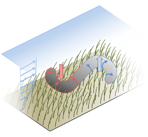
Aquatic ecosystems constitute a topic of high relevance due to their abundance and their various roles on different scales, ranging from the quality of drinking water taken from the local river to the large-scale impact on climate change (Costanza et al. Reference Costanza, d'Arge, de Groot, Farber, Grasso, Hannon, Limburg, Naeem, O'Neill and Paruelo1997; Jeppesen et al. Reference Jeppesen, Søndergaard, Søndergaard and Christoffersen1998). The interactions between the flow and the flexible plants in an aquatic canopy, as displayed in figure 1(a), play a central role in hydraulics as well as transport of sediment, nutrients and pollutants (Jeppesen et al. Reference Jeppesen, Søndergaard, Søndergaard and Christoffersen1998; Nepf Reference Nepf2012). Such flows over and through natural vegetation are extremely difficult to measure experimentally, especially inside the canopy, due to limited optical access (Nezu & Sanjou Reference Nezu and Sanjou2008). Here, numerical simulations are advantageous to provide detailed information. The numerical study of canopy flows is a rather young research field, in particular when it comes to resolving individual structures. Indeed, scale-resolving flow data are required, since, for example, little is known about the three-dimensional nature of turbulent structures in canopy flows. This lack of knowledge is addressed in the present work by conducting highly resolved simulations of a model canopy flow, with a sample picture shown in figure 1(b).

Figure 1. Seagrass meadow as an example of a dense submerged canopy. (a) Real configuration found in nature (Adobe 2018). (b) A simplified model canopy employed for the present scale-resolving simulations. The model vegetation is made out of flexible blades of equal properties, arranged uniformly in the fluid domain (same spacing in the  $x$- and $z$-directions). This rendering depicts a snapshot from a simulation with domain size $12H\times H\times 6H$, where $H$ is the flow depth.
Nepf (Reference Nepf2012) provides a comprehensive overview of canopy flows which can be classified into terrestrial and aquatic canopies. The rigidity of terrestrial plants, e.g. cereal plants, is usually higher compared to aquatic plants since aquatic canopies are supported by buoyancy to act against gravity, which is not the case for terrestrial plants. Consequently, the deflection of single plants is smaller in terrestrial canopies (Raupach, Finnigan & Brunei Reference Raupach, Finnigan and Brunei1996; Dupont et al. Reference Dupont, Gosselin, Py, de Langre, Hemon and Brunet2010). Their low rigidity aids aquatic plants to lower drag by changing their geometry when subjected to hydrodynamic loads, a phenomenon commonly termed reconfiguration (Vogel Reference Vogel1994; de Langre Reference de Langre2012). The reconfigured geometry modifies the fluid motion resulting in a strongly coupled two-way fluid–structure interaction (FSI).
Canopies can be further classified by their submergence. Atmospheric canopies are located at the bottom of an atmospheric boundary layer thicker by orders of magnitude than the vegetation layer and not exhibiting a sharp upper boundary, so that the submergence is extremely high. For aquatic canopies the situation is more complex as the water depth is finite and usually restricted to moderate depths. From a fluid mechanics point of view the ratio between the water depth  $H$ and the height of plants after reconfiguration $L^{\ast }$ is used to distinguish between deep submergence with $H/L^{\ast }>10$ and shallow submergence with $H/L^{\ast }<5$, completed by a regime of intermediate submergence in between (Nepf Reference Nepf2012). Due to the requirement of sunlight, shallow submergence is common in aquatic systems. While deeply submerged canopies show similarities to terrestrial canopies for sufficiently large ratios $H/L^{\ast }$, the situation is different for aquatic canopies with shallow submergence, revealing substantially different turbulent structures (Nepf & Vivoni Reference Nepf and Vivoni2000) which are not affected by large-scale outer-layer turbulent structures as observed in atmospheric boundary layers (Dupont et al. Reference Dupont, Gosselin, Py, de Langre, Hemon and Brunet2010).
Another important parameter is the density of the canopy, measured by the frontal area of vegetation elements per bed area  ${{\lambda }^{\ast }}$, the frontal area index. In the present case featuring blades of constant width $W$ and a spacing $\Delta S$ between individual plants it is
 \begin{equation} {{\lambda}^{{\ast}}} = \frac{L^{{\ast}} W}{\Delta S^2}. \end{equation}
When multiplied with the drag coefficient  $C_{d}$ one obtains a measure for the flow resistance of the canopy. While the flow over and through sufficiently sparse canopies ( $C_{d}{{\lambda }^{\ast }} < 0.1$) closely resembles common boundary layer flows, dense canopies ( $C_{d}{{\lambda }^{\ast }} > 0.23$) generate a pronounced mixing layer at their top making the flow prone to Kelvin–Helmholtz (KH) instabilities (Nepf Reference Nepf2012). Analysis of corresponding turbulent structures in dense shallow canopies of rigid elements shows that the flow is dominated by strong sweep and ejection events in the mixing layer (Okamoto & Nezu Reference Okamoto and Nezu2010a). Depending on the degree of reconfiguration of vegetation elements, the interaction between these coherent structures and the canopy results in different flow patterns (Carollo, Ferro & Termini Reference Carollo, Ferro and Termini2005; Okamoto & Nezu Reference Okamoto and Nezu2009). In this regard, the Cauchy number $Ca$ is an important dimensionless number to distinguish between different types of vegetation. It is defined as
 \begin{equation} Ca = \frac{(\rho_{f}/2) U^2 W L}{E_{{s}} I/L^2}, \end{equation}
with the fluid density  $\rho_f$, the bulk velocity U, and the length L and flexural rigidity $E_{{s}} I$ of an individual vegetation element, where $E_{{s}}$ is the Young's modulus of the material and $I$ the second moment of area. The Cauchy number represents the ratio between drag forces and restoring elastic forces, so that a high degree of reconfiguration relates to large values of $Ca$. Often, a nominal $C_{d}$ is included in the numerator of the definition of $Ca$ to emphasize this relation. Different mechanisms of fluid–structure interaction can be observed with increasing $Ca$, as illustrated in figure 2. For $Ca\ll 1$ vegetation elements remain erect (Luhar & Nepf Reference Luhar and Nepf2011). A mixing layer occurs at the top of the canopy (figure 2a) with KH vortices generated and convected in streamwise direction. At a certain value of $Ca$ the elements start to sway independently and with small amplitudes, a regime called ‘gently swaying’ (figure 2b). For larger $Ca$ the elements are more reconfigured and can exhibit highly coherent waving motions, a phenomenon called monami (Japanese: mo = aquatic plant, nami = wave; Ackerman & Okubo Reference Ackerman and Okubo1993; Okubo & Levin Reference Okubo and Levin2001) as sketched in figure 2(c). Very large values of $Ca$ result in a substantial reconfiguration with elements mainly aligned in streamwise direction (figure 2d). The mixing layer and the corresponding KH vortices are suppressed since the canopy top is fully covered by reconfigured elements. This prevents most of the momentum exchange in vertical direction.
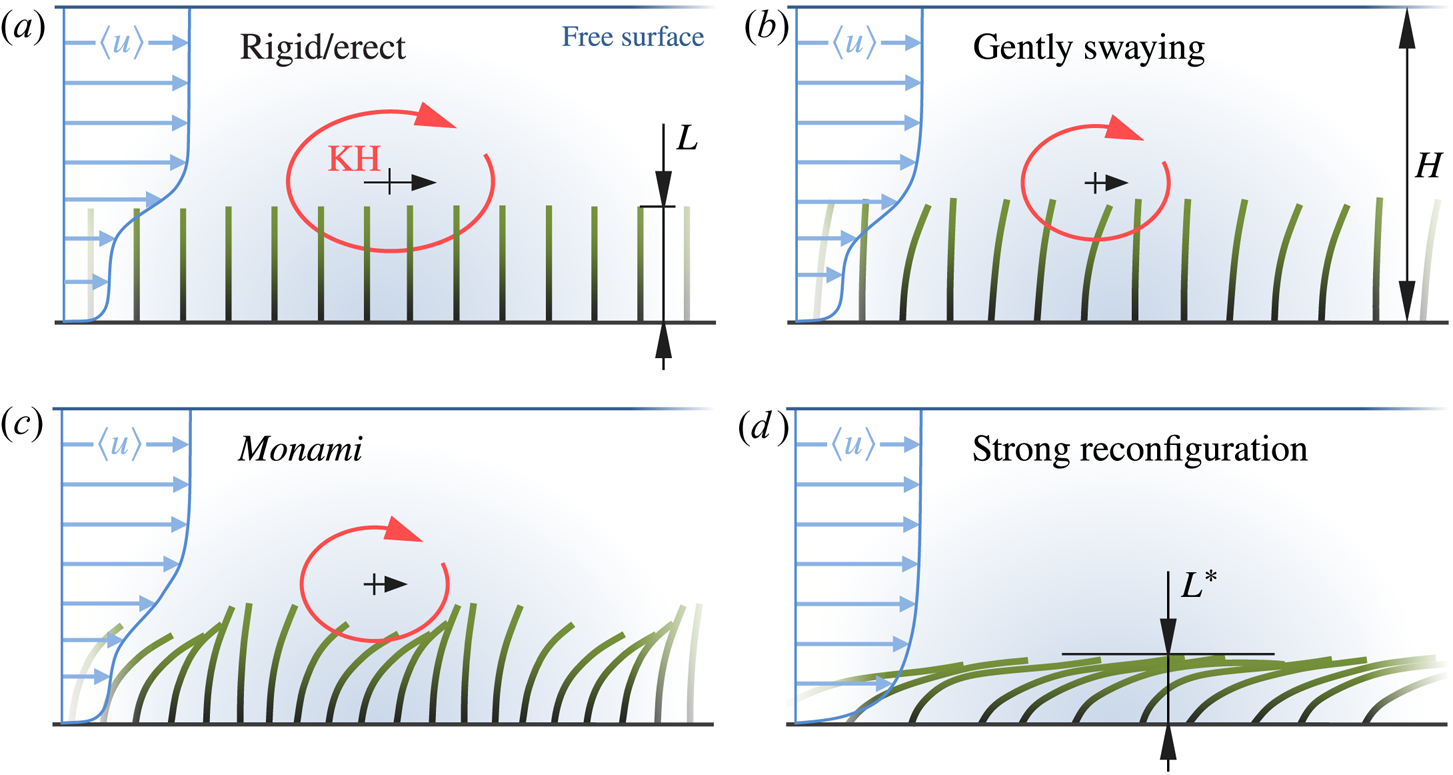
Figure 2. Influence of the Cauchy number  $Ca$ on the FSI of dense shallowly submerged canopies. Pictures drawn according to Okamoto & Nezu (Reference Okamoto and Nezu2010a) and Okamoto, Nezu & Sanjou (Reference Okamoto, Nezu and Sanjou2016). The value of $Ca$ is well below one in (a) and increases in (b–d), accompanied by an increased mean reconfiguration of the vegetation elements (green) and substantially different regimes of fluid and structure dynamics. No KH vortex (red) is observed in the regime of strong reconfiguration (d).
Coherent flow structures generated by the shear layer are only one part of a number of particular features at a hierarchy of scales (Nikora et al. Reference Nikora, Cameron, Albayrak, Miler, Nikora, Siniscalchi, Stewart and O'Hare2012), illustrated in figure 3. They range from the sub-plant scale over the plant scale where wakes of individual plants are observed, up to the canopy scale featuring the shear layer between the canopy and the outer flow and the scale of the boundary layer above the canopy. Additionally, in natural rivers aquatic plants are often separated in patches, so that the patch scale is also important for some processes (Nikora et al. Reference Nikora, Cameron, Albayrak, Miler, Nikora, Siniscalchi, Stewart and O'Hare2012; Cornacchia et al. Reference Cornacchia, van de Koppel, van der Wal, Wharton, Puijalon and Bouma2018). To date, the coexistence and interaction of these different scales is not fully understood and constitutes a major challenge for experimental studies and numerical investigations.

Figure 3. Illustration of flow features on different length scales as sketched and labelled by Nikora et al. (Reference Nikora, Cameron, Albayrak, Miler, Nikora, Siniscalchi, Stewart and O'Hare2012). (1) Depth-scale shear-generated turbulence, (2) canopy-height-scale turbulence at the upper boundary of the vegetation canopy, (3) small-scale turbulence associated with flow separation from stems, (4) small-scale turbulence within local boundary layers attached to leaves or stem surfaces, (5) small-scale turbulence in the wake of plant leaves, (6) fluctuations due to plant leaf waviness.
1.2. Experimental studies of canopy flows
Due to the wide range of scales in aquatic canopies, experimental studies range from field studies in real rivers to laboratory experiments with abstracted model canopies. The former generally address the patch scale or larger scales (Sukhodolova Reference Sukhodolova2008; Nikora et al. Reference Nikora, Cameron, Albayrak, Miler, Nikora, Siniscalchi, Stewart and O'Hare2012) while smaller scales are generally not addressed since this is more convenient in laboratory flumes. Here, model canopies can be made of natural plants (Järvelä Reference Järvelä2005; Puijalon et al. Reference Puijalon, Léna, Rivière, Champagne, Rostan and Bornette2008), but due to the difficulties of conducting long term experiments with living plants and to focus on the fundamental effects, most of the studies in flumes were conducted with model plants (Kouwen & Unny Reference Kouwen and Unny1973; Ghisalberti & Nepf Reference Ghisalberti and Nepf2002; Wilson et al. Reference Wilson, Stoesser, Bates and Pinzen2003; Okamoto & Nezu Reference Okamoto and Nezu2010a; Siniscalchi, Nikora & Aberle Reference Siniscalchi, Nikora and Aberle2012). As demonstrated in Luhar & Nepf (Reference Luhar and Nepf2011) and Rominger & Nepf (Reference Rominger and Nepf2014) model plants, usually shaped as cylinders or thin blades, are indeed able to capture the behaviour of living plants, such as drag forces and reconfiguration. Furthermore, the flexural rigidity of model plants can be chosen more easily such that a desired Cauchy number is obtained. Shallow canopies made of rigid cylinders or blades were experimentally studied in Nezu & Sanjou (Reference Nezu and Sanjou2008), Okamoto & Nezu (Reference Okamoto and Nezu2010a), Lu & Chen (Reference Lu and Chen2014) and Okamoto et al. (Reference Okamoto, Nezu and Sanjou2016), while flexible model plants were employed in Ghisalberti & Nepf (Reference Ghisalberti and Nepf2006), Okamoto & Nezu (Reference Okamoto and Nezu2010a), Marjoribanks et al. (Reference Marjoribanks, Hardy, Lane and Parsons2014) and Le Bouteiller & Venditti (Reference Le Bouteiller and Venditti2015). As an example, Ghisalberti & Nepf (Reference Ghisalberti and Nepf2006) modelled each plant by a rigid stem with highly flexible plastic blades attached, mimicking the typical morphology of eelgrass.
Unfortunately, obtaining spatially detailed measurements inside the canopy is particularly difficult due to limited optical access. This also holds for data acquisition of the plant motion. Thus, most of the experimental studies mentioned above focused on drag forces, exerted by the canopy on the flow as a whole in relation to the reconfigured canopy height. Only very few experimental studies of flexible canopies were conducted with simultaneous measurements of blade motion and fluid flow (Okamoto & Nezu Reference Okamoto and Nezu2009; Okamoto et al. Reference Okamoto, Nezu and Sanjou2016). This, however, is a prerequisite for a deeper understanding of hydrodynamic processes in canopy flows. Consequently, data acquisition must be complemented by numerical studies which are discussed in the following.
1.3. Numerical simulations of canopy flows in the literature
Depending on the scales of interest different numerical models have been employed for the simulation of canopy flows. In most cases it was deemed sufficient to use a homogenized representation of the canopy as a whole, especially when interested in average quantities, such as mean velocity profiles, Reynolds stresses, etc. For terrestrial canopies, solving the Reynolds-averaged Navier–Stokes (RANS) equations using a homogenized drag law is state of the art (Barrios-Pina et al. Reference Barrios-Pina, Ramírez-León, Rodríguez-Cuevas and Couder-Castaneda2014). In submerged aquatic canopies, however, the reconfiguration is larger so that the RANS approach must be supplemented with the deformability of the canopy (Velasco, Bateman & Medina Reference Velasco, Bateman and Medina2008; Dijkstra & Uittenbogaard Reference Dijkstra and Uittenbogaard2010). When interested in the nature of coherent structures, eddy-resolving approaches, such as large eddy simulation (LES), are employed to resolve large-scale coherent vortex structures (Li & Xie Reference Li and Xie2011; Gac Reference Gac2014; Marjoribanks et al. Reference Marjoribanks, Hardy, Lane and Parsons2017). For the sake of simplicity, canopies can still be modelled as time-independent homogeneous continua. Shaw & Schumann (Reference Shaw and Schumann1992) were the first in this direction proposing a relation for the drag force proportional to the canopy density. A time-dependent flexible homogenized canopy in an LES was realized by Dupont et al. (Reference Dupont, Gosselin, Py, de Langre, Hemon and Brunet2010) for a terrestrial grainfield.
Besides a homogenized representation of vegetation, LES have also been used to study channel flows with regularly arranged, geometrically obstacles of various shapes. Earlier studies are (Mathey, Fröhlich & Rodi Reference Mathey, Fröhlich and Rodi1999; Kanda, Moriwaki & Kasamatsu Reference Kanda, Moriwaki and Kasamatsu2004; Stoesser, Kim & Diplas Reference Stoesser, Kim and Diplas2010) with many others in more recent years. Further work in this direction, but with a clear focus on aquatic canopy flow, was undertaken in the group of Okamoto & Nezu (Reference Okamoto and Nezu2010b) simulating an experiment with rigid blades conducted in the same group (Nezu & Sanjou Reference Nezu and Sanjou2008). Due to the fine spatial and temporal resolution required for these investigations, geometry-resolving simulations of the fluid–structure interaction in canopy flows are extremely costly, especially when reliable statistical data are to be accumulated over a longer time interval.
The coupling of fluid and structures in a numerical simulation can be established by means of very different approaches ranging from a body-fitted grid to an immersed boundary method (IBM) (Bungartz & Schäfer Reference Bungartz and Schäfer2006; Sotiropoulos & Yang Reference Sotiropoulos and Yang2014). For the latter group it is comparatively easy and computationally efficient to impose boundary conditions for complex time-dependent geometries, as needed for flexible structures of low rigidity.
So far, only very few simulations have been undertaken addressing the flow over arrays of flexible structures of canopy-like geometry. Yang, Preidikman & Balaras (Reference Yang, Preidikman and Balaras2008) employed an IBM to perform two-dimensional simulations of the flow around  $16$ rigid cylinders mounted elastically to the bottom wall. Yusuf, Karim & Osman (Reference Yusuf, Karim and Osman2009) computed the flow around $10$ triangular and round structures undergoing only small deformations in a uniform cross-flow by means of an adaptive mesh technique. Recently, IBM were combined with structure solvers able to represent large deformations (Sotiropoulos & Yang Reference Sotiropoulos and Yang2014; Tian et al. Reference Tian, Dai, Luo, Doyle and Rousseau2014; Kim, Lee & Choi Reference Kim, Lee and Choi2018). The latter one, for example, applied the method to a single flexible blade in cross-flow. Only very few numerical studies could be found in the literature reporting on simulations of large numbers of highly flexible structures. To the knowledge of the authors, the work of Marjoribanks (Marjoribanks Reference Marjoribanks2013; Marjoribanks et al. Reference Marjoribanks, Hardy, Lane and Parsons2014) provides the most advanced simulation of an entire canopy with up to $300$ individual flexible elements in cross-flow. The geometrical description of the structures, however, is simplified by using a porosity distribution and the level of resolution is below the state of the art achieved for simulations of canopies with rigid structures (e.g. Okamoto & Nezu Reference Okamoto and Nezu2010b), or for simulations of single flexible structures undergoing large deformations (e.g. Tian et al. Reference Tian, Dai, Luo, Doyle and Rousseau2014). In fact, recurrence to simpler models is employed to alleviate the high cost for a full canopy mentioned above. Another numerical study addressing an entire canopy is (Gac Reference Gac2014), but the agreement with the corresponding experiment is not as desired. The lack of numerical studies of canopies with flexible elements results from the fact that simulating a whole canopy with individual structures being resolved is methodologically very complex and requires an extremely efficient, tailored numerical method. With the FSI approach employed in the present work this gap is closed and highly resolved simulations of canopies with hundreds of structures are possible.
1.4. Research questions and structure of the paper
In the present study, LES of a suitably designed model canopy are reported and analysed in physical terms focussing on scales (1)–(3) defined in figure 3 for a situation exhibiting the monami phenomenon (figure 2c). In particular, the hydrodynamic coupling between the flow and the slender flexible blades is addressed to answer the following questions: How is the fluid flow over and through a canopy affected by the flexibility of the blades? What is the relation between the characteristics of the blade motion and the characteristics of the fluid motion? Which kind of three-dimensional coherent structures are observed and what is their impact? To address these questions a numerical method will be employed which has recently been developed by the present authors (Tschisgale & Fröhlich Reference Tschisgale and Fröhlich2020) and is recalled in § 2. Section 3 then defines the physical configuration addressed here and provides the numerical parameters. In § 4 various instantaneous and statistical quantities are presented, generating new insight into the dynamics of a typical canopy flow. On this basis a prototypical understanding of coherent structures in this situation is developed in § 5. Finally, § 6 assembles conclusions and perspectives.
2. Physical and numerical model
The present paper is devoted to the physical analysis of a canopy flow, rather than numerical issues. This section provides the required information on the algorithm employed which is based on earlier work of the present authors (Kempe & Fröhlich Reference Kempe and Fröhlich2012; Tschisgale, Kempe & Fröhlich Reference Tschisgale, Kempe and Fröhlich2017, Reference Tschisgale, Kempe and Fröhlich2018; Tschisgale, Thiry & Fröhlich Reference Tschisgale, Thiry and Fröhlich2019). A very detailed description with numerous validations is provided in Tschisgale & Fröhlich (Reference Tschisgale and Fröhlich2020).
2.1. Fluid phase
The physical problem addressed consists of a Newtonian viscous fluid of constant density interacting with an array of elastic blades. The governing equations for the fluid motion are the unsteady three-dimensional Navier–Stokes equations
 \begin{gather} \frac{\partial{\boldsymbol{u}}}{\partial{t}} + \boldsymbol{\nabla}\boldsymbol{\cdot}(\boldsymbol{u}\otimes\boldsymbol{u}) = \frac{1}{\rho_{{f}}}\boldsymbol{\nabla}\boldsymbol{\cdot}{{\boldsymbol{\sigma}}}+\boldsymbol{f}, \end{gather}
 \begin{gather}\boldsymbol{\nabla}\boldsymbol{\cdot}\boldsymbol{u} = 0, \end{gather}
where  $\boldsymbol {u}=(u,v,w)^{\textrm {T}}$ is the velocity vector in Cartesian components along the Cartesian coordinates $x,y,z$, while $t$ represents the time, $\rho _{{f}}$ the fluid density, $\,\boldsymbol {f}$ a mass-specific force and ${{\boldsymbol {\sigma }}}$ the hydrodynamic stress tensor
 \begin{equation} {{\boldsymbol{\sigma}}} ={-}p \mathbb{I} + \mu_{{f}} (\boldsymbol{\nabla} \boldsymbol{u} + \boldsymbol{\nabla} \boldsymbol{u}^{\rm T}), \end{equation}
with  $p$ the pressure, $\mu _{{f}}=\rho _{{f}} \nu _{{f}}$ the dynamic viscosity, $\nu _{{f}}$ the kinematic viscosity and $\mathbb {I}$ the identity matrix. The Navier–Stokes equations (2.1) are solved with the in-house code PRIME which is based on a second-order finite volume approach on a staggered Cartesian Eulerian grid with constant grid step size $\Delta x$ in all directions for the spatial discretization and a semi-implicit second-order scheme for the time integration (Kempe & Fröhlich Reference Kempe and Fröhlich2012; Tschisgale et al. Reference Tschisgale, Kempe and Fröhlich2017, Reference Tschisgale, Kempe and Fröhlich2018). In the present application a direct numerical simulation (DNS) with a grid fine enough to capture all turbulent fluctuations down to the Kolmogorov scale is not feasible with presently available resources and not needed for this investigation, as demonstrated below. Hence, an LES approach is employed using the Smagorinsky subgrid-scale model (Smagorinsky Reference Smagorinsky1963) with a global Smagorinsky constant $C_{s}$.
2.2. Structural part
Elastic blades are considered, with their length  $L$ far longer than their width $W$ and their thickness $T$, again, much smaller than their width, so that they constitute a particular kind of beam. To model such blades a certain number of approximations allows replacing the fully three-dimensional representation of the elastic body by a one-dimensional rod model. Several models of this type exist. The one applied here is the geometrically exact Cosserat rod model, which is suitable for rods undergoing large deflections (Simo Reference Simo1985; Antman Reference Antman2005). The corresponding differential equations of motion are
 \begin{gather} \rho_{{s}} A \frac{\partial^2{\boldsymbol{c}}}{\partial t^2} = \frac{{\mathop {\boldsymbol f}\limits^{\Delta}}}{\partial Z} + {\mathop {\boldsymbol f}\limits^{\nabla}}, \end{gather}
 \begin{gather}\rho_{{s}}{\boldsymbol{\mathsf{I}}} \boldsymbol{\cdot} \frac{\partial{\boldsymbol \omega}}{\partial t} + {\boldsymbol{\omega}} \times \rho_{{s}}{\boldsymbol{\mathsf{I}}} \boldsymbol{\cdot} {\boldsymbol{\omega}} = \frac{{\mathop {\boldsymbol m}\limits^{\Delta}}}{\partial Z} + \frac{\partial{\boldsymbol{c}}}{\partial Z} \times {\mathop {\boldsymbol f}\limits^{\nabla}} + {\mathop {\boldsymbol m}\limits^{\nabla}}, \end{gather}
where  $\boldsymbol {c}$ is the position vector to a point on the centreline, and $Z$ the corresponding arc length coordinate. The motion of the centreline is governed by (2.3a) and depends on the internal forces ${\mathop {\boldsymbol f}\limits^{\Delta}}$ and the external forces ${\mathop {\boldsymbol f}\limits^{\nabla}}$. With the Cosserat rod model, the cross-sections of the blade are assumed to be rigid and plane throughout the deformation (Simo Reference Simo1985; Antman Reference Antman2005). Their local angular velocity $\boldsymbol {\omega }$ depends on the internal forces ${\mathop {\boldsymbol f}\limits^{\Delta}}$ and the internal moments ${\mathop {\boldsymbol m}\limits^{\Delta}}$, as well as the external moments ${\mathop {\boldsymbol f}\limits^{\nabla}}$, as described by (2.3b), with $\boldsymbol{\mathsf{I}}$ the tensor of inertia in the global Eulerian frame. The blades considered here have constant geometrical properties, i.e. constant cross-sectional areas $A$, constant material properties, such as the density $\rho _{{s}}$, and the same linear viscoelastic material of Kelvin–Voigt type over their entire length. With these assumptions, the equations of motion (2.3a) and (2.3b) are solved numerically according to Lang, Linn & Arnold (Reference Lang, Linn and Arnold2011). The centreline is decomposed into $N_{{e}}$ one-dimensional segments of equal length $L_{{e}} = L/N_{{e}}$. A finite-difference method and a special description of the rotations of the cross-sections by quaternions are then employed yielding a highly efficient algorithm (Tschisgale & Fröhlich Reference Tschisgale and Fröhlich2020).
2.3. Coupling of fluid and blades
The physical coupling of the continuous fluid phase and the blades is accomplished by the no-slip condition. While the physical value of the cross-sectional area  $A$ is finite in the Cosserat rod model, the geometry of the blades considered here is such that their thickness is substantially smaller than their width. Hence, for the coupling to the fluid the thickness of the blades is assumed to vanish. Numerically, the coupling is realized by an IBM. Each embedded blade is represented by $N_{{e}}$ planar elements, the same number as used for the discretization of (2.3), having a length $L_{{e}}$, a width $W$, and zero thickness. Lagrangian marker points are distributed over each segment in square arrangement with $N_{L_{{e}}}$ points in longitudinal and $N_W$ points in lateral direction. At the position of each marker point an artificial force $\boldsymbol {f}_{\textit{IBM}}$ is added to the momentum balance of the fluid (2.1a). This source term is determined in each time step by the so-called direct forcing approach (Mohd-Yusof Reference Mohd-Yusof1997; Fadlun et al. Reference Fadlun, Verzicco, Orlandi and Mohd-Yusof2000; Tschisgale et al. Reference Tschisgale, Kempe and Fröhlich2018) to enforce the no-slip condition at the blades. This involves interpolation of the fluid velocity to the marker points, computation of the source term at the marker points, and spreading of the source back to the Eulerian grid. Both, interpolation and spreading are accomplished using a so-called smoothed delta function $\delta _h(\boldsymbol {r})$, where $\boldsymbol {r}=(r_x,r_y,r_z)^{{\rm T}}=\boldsymbol {x}_l-\boldsymbol {x}_{ijk}$ is the distance between a Lagrangian marker $\boldsymbol {x}_l$ and an Eulerian grid point $\boldsymbol {x}_{ijk}$. The three-dimensional function $\delta _h$ is generated by the tensor product of three one-dimensional functions, i.e. $\delta _h(\boldsymbol {r})=\delta _h^{\textit{1D}}(r_x) \ \delta _h^{\textit{1D}}(r_y) \ \delta _h^{\textit{1D}}(r_z)$. Furthermore, $\delta _h^{\textit{1D}}(r_x)=\varPhi (r)/h$ and $r=r_x/h$, etc., with $h$ characterizing the width of $\delta _h^{\textit{1D}}$. Here, the function $\varPhi$ is chosen according to the work of Roma, Peskin & Berger (Reference Roma, Peskin and Berger1999) which ensures a good balance between numerical efficiency and smoothing properties. More details on the immersed boundary coupling can be found in Tschisgale et al. (Reference Tschisgale, Kempe and Fröhlich2018). A detailed description of the IBM for blades of vanishing thickness together with a validation of each ingredient and a discussion of its efficiency is provided in Tschisgale & Fröhlich (Reference Tschisgale and Fröhlich2020).
Besides the interaction between fluid and blades, flexible blades in a canopy can collide with each other. A corresponding modelling approach was developed and validated by the present authors in Tschisgale et al. (Reference Tschisgale, Thiry and Fröhlich2019).
3. Model canopy and numerical set-up
3.1. Physical set-up of the model canopy
The model canopy consists of an array of identical, strip-shaped blades with vanishing thickness but finite rigidity, fixed to the bottom wall of the simulation domain. This yields a parameter space of 11 physical parameters, resulting in 8 independent dimensionless numbers. To find appropriate sets of parameters covering the physics of real canopies at different regimes is a formidable task. In the present study the conditions were chosen according to the experiments of Okamoto & Nezu (Reference Okamoto and Nezu2010a) who investigated a variety of shallowly submerged model canopies. These experiments were conducted using a tilting flume with a length of  $10\ \textrm{m}$ and a width of $0.4\ \textrm {m}$. The vegetation elements were made of polyester overhead projector (OHP) transparencies and arranged over a length of $9\ \textrm{m}$ in streamwise direction and the full channel width. Mean velocity profiles and Reynolds stress distributions are provided in (Okamoto & Nezu Reference Okamoto and Nezu2010a) for different submergence depths and Cauchy numbers, making the experiment ideally suited for a direct comparison with the simulation and thus providing a means of validation. Here, one case at a moderate Cauchy number was selected as it exhibits the monami phenomenon (figure 2c). The related three-dimensional turbulent flow structures are very difficult to measure, so that the present simulation data can be used to investigate the physical mechanisms behind this phenomenon.
All relevant properties of the fluid and the blades are assembled in table 1. The blades are mounted in an in-line arrangement, illustrated in figure 4, defined by the distances  $\Delta S_x$ and $\Delta S_z$ in the streamwise and spanwise directions, respectively. As in the experiment, a square arrangement is used here with $\Delta S=\Delta S_x=\Delta S_z$. One complete set of eight independent dimensionless numbers is presented in table 2.
Table 1. Physical parameters defining the shallowly submerged canopy, according to Okamoto & Nezu (Reference Okamoto and Nezu2010a), simulated in the present work.


Figure 4. Sketch of the canopy investigated and definition of parameters as well as boundary conditions employed in the simulation.
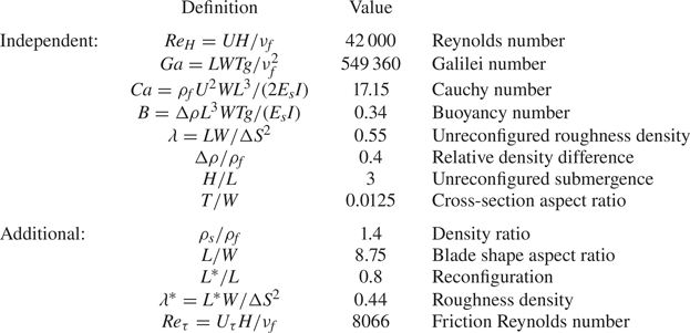
Table 2. Independent dimensionless numbers based on the physical parameters in table 1, with  $\Delta \rho =(\rho _{{s}}-\rho _{{f}})$, and additional numbers resulting from these or from the simulation result.
Regrettably, several important parameters were not provided in the paper of Okamoto & Nezu (Reference Okamoto and Nezu2010a), but could be partially reconstructed by the present authors from a previous publication of the same group (Nezu & Sanjou Reference Nezu and Sanjou2008). For instance, the number of blades fixed to the channel bottom as well as their spacings in the streamwise and spanwise directions are missing in Okamoto & Nezu (Reference Okamoto and Nezu2010a). Two years earlier, Nezu & Sanjou (Reference Nezu and Sanjou2008) used an equal spacing of  $\Delta S = 32\ \textrm {mm}$ in a very similar experimental set-up with an array of rigid blades and a frontal area per canopy volume of $a=W/\Delta S^2 \approx 7.8\ \textrm {m}^{-1}$. Since this value of $a$ is nearly equivalent to the value provided in Okamoto & Nezu (Reference Okamoto and Nezu2010a), it is assumed here that the same spacing of $32\ \textrm{mm}$ was also used in the latter reference. This choice is corroborated by a later publication of the same authors (Okamoto et al. Reference Okamoto, Nezu and Sanjou2016), where a value of $32\ \textrm {mm}$ is provided for spanwise and lateral blade spacings in experiments that appear to be identical to those in Okamoto & Nezu (Reference Okamoto and Nezu2010a). Another issue concerns the material properties of the OHP transparencies, especially the flexural rigidity $E_{{s}} I$ and the mass density $\rho _{{s}}$. In Okamoto & Nezu (Reference Okamoto and Nezu2010a), the rigidity is provided with a value of $E_{{s}} I=73\ \mathrm {\mu }\textrm {N}\ \textrm {m}^{2}$ yielding a Young's modulus of $E_{{s}} = 109.5\ \textrm {GN}\ \textrm {m}^{-2}$ for rectangular cross-sections with $I=WT^3/12$. This value, however, is far too high for OHP transparencies usually made of thermoplastic polymer materials, e.g. polyvinyl chloride (PVC) or polyethylene terephthalate (PET). To resolve the issue, the value of $E_{{s}}$ was adjusted in a preliminary simulation using an iterative procedure taking the average reconfigured height of the deflected blades $L^{\ast }$ as the target. The value $L^{\ast }/L = 0.8$ given in Okamoto & Nezu (Reference Okamoto and Nezu2010a) then resulted in $E_{{s}} = 4.8\ \textrm {GN}\ \textrm {m}^{-2}$. Especially for PVC, PET or similar polymers a wide range of values for $E_{{s}}$ can be found in the literature ranging from $E_{{s}} = 2.4\ \textrm {GN}\ \textrm {m}^{-2}$ to $11\ \textrm {GN}\ \textrm {m}^{-2}$ (Titow Reference Titow1984; Berins Reference Berins1991; Brydson Reference Brydson1999; Harper Reference Harper2000; The Engineering ToolBox 2018), depending on the specific material composition and the thermo-mechanical treatment during manufacturing. On this background the value $E_{{s}} = 4.8\ \textrm {GN}\ \textrm {m}^{-2}$ obtained here for the blades used by Okamoto & Nezu (Reference Okamoto and Nezu2010a) seems realistic. The value of $\rho _{{s}}$, on the other hand, is entirely missing in Okamoto & Nezu (Reference Okamoto and Nezu2010a) and Okamoto et al. (Reference Okamoto, Nezu and Sanjou2016). Therefore, $\rho _{{s}} = 1400\ \textrm {kg}\ \textrm {m}^{-3}$ is used here, in accordance with the span of values reported for PVC and PET in the literature, ranging from $\rho _{{s}} = 1300\ \textrm {kg}\ \textrm {m}^{-3}$ to $1450\ \textrm {kg}\ \textrm {m}^{-3}$ (Titow Reference Titow1984; GESTIS 2018).
3.2. Numerical set-up
In the experiment the water depth was  $0.21\ \textrm {m}$ and the measurement zone was positioned $7\ \textrm {m}$ downstream of the leading edge of the artificial canopy to ensure fully developed flow (Nezu & Sanjou Reference Nezu and Sanjou2008; Okamoto & Nezu Reference Okamoto and Nezu2010a). Sidewall effects could be excluded since a two-dimensional mean flow was observed above the canopy in the measurement zone of width $\Delta S_z$ surrounding the centre plane $z=L_z/2$ (Nezu & Sanjou Reference Nezu and Sanjou2008). For the numerical model this justifies the application of periodic boundary conditions in spanwise direction. The present study addresses the fully developed flow, so that periodic boundary conditions were applied in the streamwise direction as well. Based on the water depth of the experiment a computational domain of $L_x \times L_y \times L_z = 1.28\ \textrm {m} \times 0.21\ \textrm {m} \times 0.64\ \textrm {m}$ was chosen. This amounts to a non-dimensional extension of approximately $6H \times H \times 3H$ in the $x$-,
$x$-,  $y$-,
$y$-,  $z$-directions, respectively, which is larger than classically used for DNS and LES of plane channel flow simulations (e.g. Moser, Kim & Mansour Reference Moser, Kim and Mansour1999). Observing that with $L^{\ast }/L=0.8$ the reconfigured canopy covers approximately 0.27 % of the domain height, the effective aspect ratio is even larger. Figure 5 compares the present domain size and the total number of grid points used with four other numerical studies of canopy flows (Okamoto & Nezu Reference Okamoto and Nezu2010b; Li & Xie Reference Li and Xie2011; Gac Reference Gac2014; Marjoribanks et al. Reference Marjoribanks, Hardy, Lane and Parsons2017). With the present choice for $L_x$ and $L_z$ the domain contains $N_{{s},x}=40$ structures in the streamwise and $N_{{s},z}=20$ structures in the spanwise direction, yielding a total of $N_{{s}}=800$ structures.

Figure 5. Horizontal domain size and total number of grid points employed for the present study and in Okamoto & Nezu (Reference Okamoto and Nezu2010b), Li & Xie (Reference Li and Xie2011), Gac (Reference Gac2014) and Marjoribanks et al. (Reference Marjoribanks, Hardy, Lane and Parsons2017). The values of  $H$ correspond to the heights of the respective domains.
At the bottom wall and at the blade surfaces a no-slip boundary condition is employed. A rigid lid condition is used at the upper boundary which is employed in almost all simulations of this type, e.g. Rodi, Constantinescu & Stoesser (Reference Rodi, Constantinescu and Stoesser2013), Vowinckel, Kempe & Fröhlich (Reference Vowinckel, Kempe and Fröhlich2014) and Vowinckel et al. (Reference Vowinckel, Jain, Kempe and Fröhlich2016). Indeed, it was verified a posteriori by assessing the computed pressure at the upper boundary that in case of a free surface deformations would remain below  $0.2\ \textrm {mm}$.
The channel is horizontal and the flow is driven by a spatially constant volume force. This represents the flow in a tilted flume very well, since the angle it would take is extremely small, and is standard practise in simulations of canopies and sediment transport (Gac Reference Gac2014; Vowinckel et al. Reference Vowinckel, Kempe and Fröhlich2014; Kidanemariam & Uhlmann Reference Kidanemariam and Uhlmann2017). The volume force is adjusted in each time step by means of a controller to impose the desired bulk velocity. After an initial transient from rest, the bulk velocity  $U=0.2\ \textrm {m}\ \textrm {s}^{-1}$ is constant and the flow fully developed.
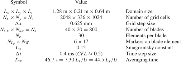
The computational domain is discretized by cubic cells of size  $\Delta x = \Delta y = \Delta z = 0.625\ \textrm {mm}$ in all directions. This results in $W/\Delta z=12.8$ grid cells over the blade width and a total number of approximately $700$ million grid cells of the Eulerian grid. Each blade is discretized with $N_{{e}}=30$ elements, and the surface of each element is covered with $N_{L_{{e}}}\times N_W = 6 \times 17$ markers.
To model the subgrid-scale turbulence a Smagorinsky constant of  $C_{s}=0.15$ was chosen, as already employed by Okamoto & Nezu (Reference Okamoto and Nezu2010b) and Gac (Reference Gac2014) for LES of canopy flows over rigid blades, and by Li & Xie (Reference Li and Xie2011) for LES of canopy flows involving flexible vegetation. Marjoribanks used $C_{s}=0.17$, which is similar as well (Marjoribanks Reference Marjoribanks2013; Marjoribanks et al. Reference Marjoribanks, Hardy, Lane and Parsons2014, Reference Marjoribanks, Hardy, Lane and Parsons2017).
Regarding the temporal discretization, the time step size was set to  $\Delta t = 0.4\ \textrm {ms}$ yielding a Courant number of $\mathit{CFL} \approx 0.5$. Averaging was started when the simulation had reached the statistically steady state. This was checked by monitoring the driving force $f_x(t)$ and the reconfiguration of the blades, verifying that their temporal behaviour was exempt of any sign related to start-up. The collection of samples was undertaken for a duration of $44.5\ T_{b}$ until one-point statistics were converged.
All relevant numerical parameters are summarized in table 3.
Table 3. Overview over numerical parameters used for the present simulation.
The Appendix contains a detailed study of the sensitivity of the results with respect to (i) grid resolution, (ii) temporal resolution, (iii) domain size and (iv) subgrid-scale coefficient  $C_{s}$. These tests show that the numerical parameters are suitable and provide reliable simulation results.
4. Data analysis and physical interpretation
The canopy defined in § 3.1 was simulated with the numerical parameters determined in § 3.2. This section reports on the instantaneous solution and various statistical quantities computed from the instantaneous data. Throughout,  $\langle \cdots \rangle$ identifies averages over $x$,
$x$,  $z$ and $t$. Whenever a different kind of averaging is meant this is indicated by an index, like $\langle \cdots \rangle _t$ for time averaging alone.
4.1. Instantaneous solution
Before addressing statistical properties it is instructive to inspect the computed flow itself, figures 6(a), 6(b), and 6(c) report instantaneous snapshots of  $u$,
$u$,  $v$ and $p$, respectively, for the same instant, each in the same three perpendicular planes. None of these graphs shows numerical oscillations or any other sign of problems with the numerical resolution of the flow.

Figure 6. Instantaneous flow quantities in the vertical planes  $z=0.48L_z$ and $x=0.5L_x$ and in the horizontal plane $y=L^{\ast }$. Broken lines indicated the intersections of these planes. Solid lines in the $xz$- and $xy$-slices mark intersections with the blades. Solid lines in the $zy$-slices outline the projected blades. (a) Streamwise velocity component $u$, (b) vertical velocity component $v$, (c) pressure $p$.
$p$.
The streamwise velocity in the horizontal plane of figure 6(a)  $y=L^{\ast }$ shows large-scale areas of positive and negative fluctuations with a characteristic size of approximately $0.5H$ to $H$ in lateral direction and approximately $2H$ in streamwise direction. They are superimposed on a small-scale pattern with small streamwise velocity when blades are present and larger velocity in between. The centre plane $z=\mathrm {const.}$ shows inclined patterns with an angle of approximately $20^{\circ }$ ( $x/H\approx 1.5,\ldots ,3$) which are known from flat plate turbulent boundary layers (Nezu & Nakagawa Reference Nezu and Nakagawa1993). This plane also shows the deflected blades and reveals that at times these can be bent downwards fairly strongly, at $x/H\approx 0.8$. The streamwise velocity is small inside the canopy in general, but can also exhibit larger values where the blades are bent downwards (e.g. $x/H\approx 0.8$), or when the outer velocity is larger than the average ( $x/H\approx 4,\ldots ,6$). Here, the picture also reveals the fine-scale turbulence, in particular scales of the size of the blade width and smaller, which correspond to feature (3) in figure 3. The plane $x=\mathrm {const.}$ shows the large size of ejections ( $z/H \approx 1.5,\ldots ,2.5$) and sweeps ( $z/H\approx 1$, $z/H\approx 2$) which can cover the entire outer flow up to the surface. Furthermore, this graph shows how the fast fluid moving downwards (cf. figure 6b) intrudes into the space between the blades ( $z/H\approx 1$), as well as the reduction of $u$ due to the presence of the blades.
Figure 6(b) shows the instantaneous vertical velocity component providing complementary information to figure 6(a). The apparent granularity of the pattern in the horizontal plane is larger here, since the elevation is  $y=L^{\ast }$, i.e. the mean reconfiguration height, with blade tips locally above and locally below this plane. Still, it can be seen that regions of $u'>0$ tend to exhibit $v'<0$ and vice versa, which will be quantified in a statistical sense below. The instantaneous values frequently go up to $0.5U$ and more. The centre plane $z=\mathrm {const.}$ shows the inclined flow feature between $x/H=1.5,\ldots ,3$ addressed above with patches of alternating signs, indicating spanwise oriented vortical motion. The local vertical velocity revealed in this plane going through a row of blades has sizable values also inside the canopy due to the upward deflection of the flow by the blades. Between the streamwise rows of blades the vertical velocity is markedly negative at several locations, as seen in the cross-plane $x=\mathrm {const.}$ of this figure around $z/H\approx 0.1,\ldots ,0.8$, where this feature reaches down to the bottom wall. This plane also shows the ejection and sweep events addressed before and, by the sign of $v$, supports this denomination.
The instantaneous pressure in figure 6(c) is much smoother than the velocity field, as it is related to the latter via its gradient. Pressure minima tend to be located in vortex centres and the plane  $z=\mathrm {const.}$ shows such a sequence of vortices along an inclined line for $x/H\approx 0.7,\ldots ,3$. On the blade high pressure is seen in this graph upstream of the blades, low pressure behind, as expected. The horizontal plane shows roughly spanwise low pressure regions for $z/H\approx 0,\ldots ,1$ around $x/H\approx 2.7$ and $4.8$, for example.
Further below the coherent vortex structures will be addressed by conditional averaging.
4.2. Mean velocity profile and Reynolds stresses
The turbulent velocity field  $\boldsymbol {u}(\boldsymbol {x},t)$ is now analysed in terms of one-point fluid statistics, i.e. mean velocity $\langle \boldsymbol {u} \rangle$ and Reynolds stresses $\langle \boldsymbol {u}'\otimes \boldsymbol {u}' \rangle$ with $\boldsymbol {u}' = \boldsymbol {u}-\langle \boldsymbol {u} \rangle$. The resulting one-point fluid statistics are displayed in figure 7. Moreover, the profiles of $\langle u \rangle$ and the turbulent shear stress $\langle u'v' \rangle$ are compared to the experimental data of Okamoto & Nezu (Reference Okamoto and Nezu2010a). The comparison shows that the mean streamwise velocity component $\langle u \rangle$ matches the experimental data well, as evident from a root mean square difference of $e_2=0.048\,U$, a mean absolute difference of $e_1=0.045U$ and a Nash–Sutcliffe efficiency of $e_{NSE}=0.99$ (Nash & Sutcliffe Reference Nash and Sutcliffe1970). The height of the inflection point of the velocity profile and the velocity magnitude at this location are very well captured by the simulation. This is in line with expectations, since the position of the inflection point coincides with the average reconfigured canopy height $L^{\ast }$ (Nepf & Vivoni Reference Nepf and Vivoni2000) which was adjusted in the simulation to the experimental observation to obtain the correct rigidity $E_{{s}} I$ of the blades as described in § 3.1 above. In terms of the Reynolds stress $\langle u'v' \rangle$ the simulation results are in good agreement with the experiment. The position of its minimum is very close to the experimental observation and the value within 5.7 %. Towards the channel bed, the $\langle u'v' \rangle$ profile deviates from the measurement below a height of approximately $0.5L$. The reason cannot be assessed with certainty here. It might result from imperfections in the measurement, from slight differences in the properties of the blades, or from tiny deviations in the mounting of the blades. Bearing in mind these issues the agreement is very satisfactory. In the free-flow region above the canopy, $\langle u'v' \rangle$ behaves linearly in the simulation as required by the momentum balance, whereas the experimental data exhibit undulations, contributing to a Nash–Sutcliffe efficiency of only $e_{NSE}=0.86$. Hence, it must be conjectured that the experimental statistics for this quantity have limited accuracy.

Figure 7. Statistical data for the fluid. (a) Normalized mean velocity profile in outer coordinates, (b) mean velocity in inner coordinates, (c) normalized streamwise fluctuations, (d) normalized Reynolds shear stress, (e) normalized vertical fluctuations, (f) normalized spanwise fluctuations; ——, present results;  $\circ$, experimental data of Okamoto & Nezu (Reference Okamoto and Nezu2010a) in (a,b,d); – – –, logarithmic fit in (a,b), according to (4.2); $\cdot \!\cdot \!\cdot \!\cdot \!\cdot \!\cdot \!\cdot$, mean reconfigured canopy height.
As described in Sanjou (Reference Sanjou2016), Poggi et al. (Reference Poggi, Porporato, Ridolfi, Albertson and Katul2004) and Ghisalberti & Nepf (Reference Ghisalberti and Nepf2006), the canopy flow over the entire channel height can be divided into three zones, as displayed in figure 8, each exhibiting different physical properties. These zones are usually classified using the mean velocity profile  $\langle u \rangle$ and the Reynolds shear stress $\langle u'v' \rangle$. The bottom region inside the canopy is termed the ‘emergent zone’ or ‘wake zone’ where the flow is dominated by wakes of individual vegetation elements, so that vertical momentum transfer is comparably small. It extends from the channel bottom to $y={y_{w}}$, with ${y_{w}}$ the elevation where $\langle u'v'\rangle$ reaches 10 % of its minimum value (Nepf & Vivoni Reference Nepf and Vivoni2000). For the present case this definition yields ${y_{w}}=0.06L$. With the corresponding velocity scale ${U_{w}} = \langle u \rangle ({y_{w}})=0.24U$ the Reynolds number characterizing the flow around the individual blades is
 \begin{equation} Re_{{s}} = \frac{{U_{w}} W}{\nu_{{f}}} \approx 400. \end{equation}
The points of flow separation from the blades are fixed and the force on the blades dominated by pressure. This situation is known to make the simulation fairly insensitive to resolution issues, provided it is beyond a certain threshold, as evidenced in the Appendix.

Figure 8. Three-zone model of an aquatic submerged canopy flow according to Sanjou (Reference Sanjou2016). The lower emergent zone is characterized by the turbulent wake of individual plants. In the mixing layer zone the flow is prone to instabilities, and turbulent fluctuations evolve to form coherent structures, e.g. KH-vortices. In the uppermost log-layer zone the free flow behaves very similarly to a boundary layer flow over a rough wall.
The subsequent zone is termed the ‘mixing layer zone’ covering the upper canopy region and the lower part of the free-flow region up to  $2 L^{\ast }$ (Nepf Reference Nepf2012). The velocity profile exhibits an inflection point at the canopy edge as a result of the shear layer generated in this zone. In particular, the maximum absolute Reynolds stress $-\langle u'v'\rangle _{min}$ is located slightly above the average canopy height $L^{\ast }$. Here, positive fluctuations $u'$ are strongly correlated with negative fluctuations $v'$ and vice versa as illustrated by juxtaposing figures 6(a) and 6(b), and proved by the data in figure 7(d), so that sweeps ( $u'>0$, $v'<0$) and ejections ( $u'<0$, $v'>0$) are the main mechanism of momentum transfer between the canopy and the free-flow region (Patton & Finnigan Reference Patton and Finnigan2012). The present statistical data are in line with this common picture, so that the detailed analysis of the vortex structures in this region provided below bear general relevance.
A third layer, located above the mixing layer, is the ‘log-layer zone’ (Sanjou Reference Sanjou2016). The velocity profile in this zone is well approximated by
 \begin{equation} \frac{\langle u \rangle^{log}(y)}{U_{\tau}} = \kappa^{{-}1} \ln\left( \frac{y-y_{m}}{y_0} \right) = \kappa^{{-}1} \ln\left( \frac{y-y_{m}}{l_{\tau}} \right) + A - \Delta U^+, \end{equation}
with the friction velocity  $U_{\tau }$, the von Kármán constant $\kappa =0.4$, the displacement height $y_{m}$, the roughness height $y_0$, the viscous unit $l_{\tau }=\nu /U_{\tau }$, the constant $A=5.2$ reflecting a smooth wall and the additional drag penalty $\Delta U^+$ due to the deformable elements. The friction velocity can be expressed in terms of the Reynolds stress $\langle u'v' \rangle$ at the canopy edge, i.e. $U_{\tau }^2=-\langle u'v' \rangle |_{{y=L^{\ast }}} \approx -\langle u'v' \rangle _{min}$ (Nepf Reference Nepf2012), which gives $U/U_{\tau } \approx 5.2$ in the present case, and a friction Reynolds number of
 \begin{equation} Re_{\tau} = \frac{U_{\tau} H}{\nu} = 8066. \end{equation}
 According to Nepf & Ghisalberti (Reference Nepf and Ghisalberti2008), the displacement height is  $y_{m}=L^{\ast }-\delta /2$, with $\delta \approx [\langle u \rangle /(\mathrm {d}\langle u \rangle / \mathrm {d}y)]_{{y=L^{\ast }}}$ and seems to increase proportionally to the average canopy height with $y_{m}/L^{\ast } \approx 0.78$ (Okamoto & Nezu Reference Okamoto and Nezu2010a). With these relations the present simulation yields $y_{m}/L^{\ast } \approx 0.69$. Minimizing $(\langle u \rangle ^{log}-\langle u \rangle )^2$ for $y>2 L^{\ast }$ with $y_0$ the free parameter to choose in (4.2), results in $y_0/ L^{\ast } = 0.112$, which is consistent with the value of $0.11$ reported by Nepf & Vivoni (Reference Nepf and Vivoni2000). The value of $y_0/ L^{\ast } = 0.112$ is equivalent to $\Delta U^+=18.9$ in (4.2). This value is in the centre of the data points when plotting $\Delta U^+$ as a function of roughness height, reported in figure 1 of Raupach, Antonia & Rajagopalan (Reference Raupach, Antonia and Rajagopalan1991). Using the frontal canopy area per volume $a=W/(\Delta S_x\Delta S_z)=7.81\ \textrm {m}^{-1}$, this gives $y_0 = 0.049 a^{-1}$ which is in agreement with the range $y_0=(0.04 \pm 0.02)a^{-1}$ observed by Nepf (Reference Nepf2012) for submerged canopies.
4.3. Reconfiguration and statistics of blade centreline
As done for the fluid velocity field a decomposition into mean and fluctuation is now performed for the array of blades. Each blade is identified by an index  $s$, with $s=1,\ldots ,N_{{s}}$. The time-dependent position of the points on the centreline of blade $s$ are ${\boldsymbol {c}_{s}} = {\boldsymbol {c}_{s}}(Z,t)$, with ${\boldsymbol {c}_{s}}(0,t) = {\boldsymbol {c}_{s,0}}$ the position of fixation on the bottom plate and $Z$ the coordinate along the centreline. The instantaneous shape of each blade, then, is given by
 \begin{equation} \boldsymbol{\mathsf{x}}_s(Z,t) = ({\mathsf{x}}_s,{\mathsf{y}}_s,{\mathsf{z}}_s)^{\textrm{T}} = {\boldsymbol{c}_{s}}(Z,t) - {\boldsymbol{c}_{s,0}}, \quad s=1,\ldots,N_{{s}} \end{equation}
(observe the different font of  ${\mathsf{x}}$, ${\mathsf{y}}$, ${\mathsf{z}}$ here). At each instant in time the average over all $N_{{s}}$ blades
 \begin{equation} \langle \boldsymbol{\mathsf{x}} \rangle_s(Z,t) = \frac{1}{N_{{s}}} \sum_{s=1}^{N_{{s}}} \boldsymbol{\mathsf{x}}_s(Z,t) \end{equation}
can be computed, which is then further averaged in time to yield  $\langle\boldsymbol{\mathsf{x}}\rangle_{s,t}$ subsequently denoted $\langle\boldsymbol{\mathsf{x}}\rangle$ for simplicity. All statistical data for the structures were collected over the time span $T_{av}$ (table 3). The non-vanishing components $\langle {\mathsf{x}} \rangle$ and $\langle {\mathsf{y}} \rangle$ of the mean blade profile are given in figure 9(a–c). The standard deviations of the fluctuations $\sqrt {\langle {\mathsf{x}}'{\mathsf{x}}'\rangle }/L$, etc., are shown in figure 9(d–f) to assess the specific type of oscillation, e.g. mode 1 bending or mixed-mode bending. No lateral reconfiguration $\langle {\mathsf{z}} \rangle$ in the homogeneous spanwise direction is obtained, and also the component $\sqrt {\langle {\mathsf{z}}'{\mathsf{z}}' \rangle }/L$ is below $1.5\times 10^{-5}$ throughout, hence negligible. This implies that the blades do not undergo any lateral motion which is a consequence of their flat cross-section, their orientation perpendicular to the mean flow and their type of arrangement in the canopy. Statistical data of the OHP-strip motion were not acquired in the experiment (Okamoto & Nezu Reference Okamoto and Nezu2010a), so that a comparison with the experiment is not possible.

Figure 9. Normalized statistics of blade motion components. (a) Mean streamwise position  $\langle {\mathsf{x}} \rangle /L$ as a function of the blade coordinate $Z/L$, (b) mean wall-normal coordinate in the same perspective, (c) average shape in laboratory coordinates, (d–f) normalized fluctuations.
Addressing the data in figure 9, it is observed that the centreline of the blades shows a pronounced reconfiguration in the streamwise direction (figure 9a–c). All fluctuations are of the same order of magnitude. This suggests that the blade motion in the  $x$- and $y$-direction is strongly coupled, which is naturally the case as a forward bending of the blade in the $x$-direction induces a $y$-deflection. The fluctuations plotted in figure 9(d–f) show that the motion of the blades is characterized by a mode 1 bending. If the blades were to oscillate, for instance, with a pronounced second bending mode, the profiles $\langle {\mathsf{x}}'{\mathsf{x}}' \rangle (Z)$, $\langle {\mathsf{x}}'{\mathsf{y}}' \rangle (Z)$ and $\langle {\mathsf{y}}'{\mathsf{y}}' \rangle (Z)$ would have inflection points at some arc length $0 < Z \le L$. Furthermore, the correlation coefficient $-\rho _{{\mathsf{x}}{\mathsf{y}}}$ is superior to $96\,\%$ throughout, removing any doubt in this respect.
This analysis reveals that the entire motion of each blade is fully described by the motion of its tip  ${\mathsf{y}}^{\ast }_s(t) = {\mathsf{y}}_s(Z=L,t)$, $s=1,\ldots ,N_{{s}}$. Any other material point on the blade performs an equivalent synchronous motion, just with a smaller amplitude. Hence, the tip height of the individual blades, ${\mathsf{y}}^{\ast }_s$, mostly denoted ${\mathsf{y}}^{\ast }$ for better readability, will be used below to investigate the dynamics of the blades.
4.4. Instantaneous blade tip motion
In the monami regime studied here the blades oscillate vigorously between an almost upright shape and a maximum deflection of their tip by approximately  $50\,\%$ of their length (figure 10). Based on the results of the previous section the tip motion of the blades is now analysed in detail as it fully represents the motion of the blades. For illustration, figure 10(a) shows this quantity over time for two blades in the same $z$-plane with maximum distance $L_x/2$ in $x$. Figure 10(b) provides the probability density function (PDF) of the tip position obtained from combined averaging over structures and time. The sample signals of the unsteady tip positions in figure 10(a) show particular characteristics. Periodic features are observed with a fairly regular pattern the frequency content of which is analysed below. The minima, i.e. the instants of largest deflection, are fairly short, with steep descents and ascents. The maxima, on the other hand are much rounder. Geometrical issues contribute to this difference, since the signal represents the vertical coordinate of the tip which changes only little upon flexion in case the blade is almost upright. Beyond the instantaneous samples, figure 10(a) shows that the ensemble-averaged canopy height $\langle {\mathsf{y}}^\ast \rangle_s$ remains approximately constant in time. Deviations of this quantity being at most $4\,\%$ with respect to the time-averaged value $\langle {\mathsf{y}} ^{\ast } \rangle$, once again, indicate that the simulation domain is sufficiently large.

Figure 10. Instantaneous and statistical data for the blade tip height  ${\mathsf{y}}^{\ast }$. (a) Instantaneous blade tip position over time for two individual blades. Here, $t=0$ is assigned the instant when averaging in time was started and $T_b=H/U$; —— blade mounted at $(x,z)=(0,L_z/2)$, $\cdot \!\cdot \!\cdot \!\cdot \!\cdot \!\cdot \!\cdot$ blade mounted at $(x,z)=(L_x/2,L_z/2)$, $-\!\cdot \!-\!\cdot \!-$ instantaneous ensemble-averaged height $\langle {\mathsf{y}}^\ast \rangle_s$, —— average height $\langle {\mathsf{y}}^{\ast } \rangle$. (b) Histogram of the tip height of all blades in the same time span as depicted in (a).
4.5. Frequencies of blade tip motion
It is now interesting to study the frequency content of the blade motion. To this end the spectrum of  ${\mathsf{y}}^{\ast }$ was computed. This was first done for each individual blade with the Hann window applied over the entire time span $T_{av}$ to prevent frequency leakage. Then the spectrum was averaged over all blades similarly to (4.5). The resulting mean spectrum is denoted $|\widehat {{\mathsf{y}}^{\ast }}|(f)$ in the following with the ensemble-averaging operator dropped for conciseness. The result is shown in figure 11(a) with the frequency $f$ normalized by the bulk frequency $f_{b}=1/T_{b}$, i.e. the inverse of the bulk flow time unit $T_{b}=H/U$.

Figure 11. Fourier spectrum of blade tip motion  $\langle |\widehat{{\mathsf{y}}^\ast}|\rangle_s(f)$ (a) in semi-logarithmic scale and (b) in double-logarithmic scale. The frequency axes are normalized by the bulk flow frequency $f_{b} = 1/T_{b}=U/H$. The second normalization is performed with the blade frequency $f_{n}$ from (4.6).
A well-pronounced dominant frequency peak can be observed at  $f_1 \approx 0.14 f_{b}$ accompanied by two harmonics of lower energy at $f_2 \approx 2 f_1$ and $f_3 \approx 3 f_1$ indicating a periodic blade motion. Indeed, as shown in figure 10 for two individual blades, the blades exhibit an oscillatory behaviour with reconfigurations mainly in the range of $0.6 < {\mathsf{y}}^{\ast }/L < 1$. At fairly regular time intervals the blades bend down abruptly, occasionally even reaching minimum heights of ${\mathsf{y}}^{\ast }/L\approx 0.4$ which is half of the average canopy height. Statistically, such events happen with a frequency $f_1$, resulting in the dominant frequency peak of figure 11(a). Plotting the averaged spectrum in logarithmic scale (figure 11b) shows that $\langle |\widehat{{\mathsf{y}}^\ast}|\rangle_s/L \propto (f/f_b)^{-1}$ for frequencies covering approximately $70\,\%$ of the total energy.
As described above the blades mainly oscillate with a mode 1 bending. The corresponding natural frequency is (Han, Benaroya & Wei Reference Han, Benaroya and Wei1999)
 \begin{equation} f_{{n}} = \frac{1.875^2}{2{\rm \pi}} \sqrt{\frac{E_{{s}} I}{mL^3}}, \end{equation}
with the flexural rigidity  $E_{{s}} I$ and the mass $m$ of the oscillating system. In the present case the mass in (4.6) is $m=m_{{s}}+m_{add}$, which is the mass of the structure $m_{{s}}$ augmented by the added mass of the surrounding fluid, $m_{add}$. The latter can be approximated by the added mass of a transversely oscillating rectangular plate which is $m_{add}=0.25{\rm \pi} \rho _{{f}} W^2 L$ for the present blade geometry (Dong Reference Dong1978). The ratio between the frequency $f_1$ and the natural frequency of the first bending mode $f_{n}$ is an important indicator of the physical cause of the periodic motion of the blades. If the large oscillation amplitude observed in the monami regime is due to a resonant system created by the fluid and the structures, the natural frequency of the blades should also be almost equal to the frequency of the entire excited system, i.e. $f_1/f_{n} \approx 1$. If, on the other hand, the blades behave like passive objects, simply following an external periodic excitation by the fluid, their natural frequency should be much larger than the lowest dominant frequency observed in the system, i.e. $f_1/f_{n} \ll 1$.
Using (4.6) the frequency ratio is evaluated to be  $f_1/f_{n} \approx 0.15$ in the present case, indicating that the dominant frequency does not result from a mechanical resonance between the fluid and the blades. Instead, rather the blades react to the external excitation by the fluid, e.g. by coherent structures acting on the blades at regular time intervals. Indeed, Okamoto and Nezu (Nezu & Sanjou Reference Nezu and Sanjou2008; Okamoto & Nezu Reference Okamoto and Nezu2010a) observed that the flow in sufficiently dense shallow canopies is dominated by sweep and ejection events at the canopy edge. The unique feature of canopies in the monami regime is that the blades react nearly instantaneously with large displacements to an increased momentum transfer caused by such events while being sufficiently stiff to increase momentum transfer in the mixing layer required to enhance sweeps and ejections. This transfer is substantially reduced if the flexibility is too high, as illustrated in figure 2(d).
From a different point of view, since vegetation elements are capable of following the surrounding fluid motion very well for small frequency ratios  $f_1/f_{n}$, they can be employed to detect or visualize coherent structures. In cases where the ratio $f_1/f_{n}$ does not completely vanish, a small time delay between the excitation by the fluid and the response of the blade may be expected. To quantify this delay for the present scenario, an additional simulation with a single blade of the same geometry and the same material properties, but subjected to a dynamic cross-flow, was performed. The computational domain measured $3L \times H \times 2L$. At the inlet plane ( $x=0$) and the outlet plane ( $x=3L$) an oscillatory horizontal flow was imposed $(u_{\infty }, 0, 0)^{\textrm {T}}$ with $u_{\infty }/U = 0.5 + 0.25 \sin (2{\rm \pi} f t)$. The frequency $f$ was chosen to be $f_1=0.15f_{n}$ to excite the blade at the dominant frequency encountered in the canopy flow. As shown in figure 12, the blade responds with a slight time delay of $\Delta t f_1\approx 0.03$.

Figure 12. Evolution of the normalized tip displacement in  $y$-direction $\Delta {\mathsf{y}}^{\ast }/L = 1-{\mathsf{y}}^{\ast }/L$ of a single blade exposed to an imposed sinusoidal cross-flow of velocity $u_{\infty }$.
This further supports the fact that the reconfiguration of the blades is a simple reaction to an increased vertical momentum transfer, generated by sweep and ejection events. Several researchers suggest that in canopy flows sweeps and ejections appear periodically in time (Bailey & Stoll Reference Bailey and Stoll2016). For the present configuration this observation can be confirmed since the averaged spectrum of the blades is governed by periodic features, as shown in figures 10 and 11.
4.6. Two-point correlations
To characterize coherent structures on the canopy scale which are responsible for an organized motion of the blades a two-point correlation analysis was performed, for both the fluid velocity as well as the reconfiguration of the blades. The spatial autocorrelation of the streamwise fluid velocity fluctuation  $u'$ is defined as
 \begin{equation} \rho_{uu}(r_x,y,r_z) = \frac{ \langle\, u'(\boldsymbol{x},t)\, u'(\boldsymbol{x}+\boldsymbol{r},t) \,\rangle} { \sqrt{ \langle (u'(\boldsymbol{x}, t))^2 \rangle \langle ( u'(\boldsymbol{x}+\boldsymbol{r},t) )^2 \rangle } }, \end{equation}
based on the fields  $u'(\boldsymbol {x},t)$ and $u'(\boldsymbol {x}+\boldsymbol {r},t)$, with the distance vector $\boldsymbol {r}=(r_x,0,r_z)^{\textrm {T}}$ in the horizontal plane accounting for the periodicity of the computational domain in $x$ and $z$. Due to averaging in time and homogeneous directions, the correlation coefficient $\rho _{uu}$ is a function of the streamwise distance $r_x/L_x \in [-0.5,0.5]$, the vertical coordinate $y$ and the spanwise distance $r_z/L_z \in [-0.5,0.5]$. Analogously, a correlation coefficient $\rho _{{\mathsf{y}}^{\ast }{\mathsf{y}}^{\ast }}$ is defined for the fluctuation of the canopy height ${{\mathsf{y}}^{\ast }}^{\prime }(t)={\mathsf{y}}^{\ast }(t)-\langle {\mathsf{y}}^{\ast } \rangle$.
Starting with the fluid velocity, figure 13 shows that the spacing between a high-speed (HS) streak and a neighbouring low-speed (LS) streak is approximately  $2H$ in streamwise direction and $0.75H$ in spanwise direction, identified from the minimum of $\rho _{uu}(r_x,H/2,0)$ and $\rho _{uu}(0,H/2,r_z)$, respectively. These lengths also correspond the mean extent of a single streak. The change from positive to negative values of $\rho _{uu}(0,H/2,r_z)$ indicates that HS-streaks are accompanied laterally by LS-streaks and vice versa. While the same effect can be observed in streamwise direction, it is far less pronounced, indicating that the extension of streaks varies more in the streamwise direction than laterally. Consequently, a periodic pattern of alternating positive and negative correlations appears for $\rho _{uu}(r_x,H/2,r_z)$, nearly vanishing at $r_x/H=3$ and $r_z/H=1.5$. While these limits coincide with the channel half-width and half-length here, an influence of the domain size can be excluded by the supplementary simulation reported for the validation of the domain size in the Appendix.

Figure 13. Two-point correlation coefficients,  $\rho _{uu}$ at the channel half-height $H/2$ and $\rho _{{\mathsf{y}}^{\ast }{\mathsf{y}}^{\ast }}$. (a) Correlation along $r_x$ in the streamwise direction. (b) Correlation along $r_z$ in the spanwise direction.
From figure 13 it is also obvious that the spatial correlation of the blade motion  $\rho _{{\mathsf{y}}^{\ast }{\mathsf{y}}^{\ast }}$ extends exactly over the same distance as the fluid motion $\rho _{uu}$. Furthermore, the entire shapes of $\rho _{uu}$ and $\rho _{{\mathsf{y}}^{\ast }{\mathsf{y}}^{\ast }}$ are even quantitatively very close. As described in § 4.5, the flexible blades react almost instantly to an increased momentum transfer caused, e.g. by sweeps and ejections. It is observed that in regions with $u'>0$ the blades are bent more strongly due to an increased drag, while being more erect in regions with $u'<0$. Figure 6(a) provides an illustration. The correlation coefficient of $\rho _{uu}$ and $\rho _{{\mathsf{y}}^{\ast }{\mathsf{y}}^{\ast }}$ gives a value of approximately $0.89$, which further supports the strong coupling between velocity streaks and reconfiguration of blades.
Moreover, the frequency associated with the streamwise coherence length  $l_{c}$ and the mean velocity at the canopy edge is $\langle u \rangle (y=L^{\ast })/l_{c} \approx 0.6\,U/(4H) = 0.15U/H$. This value provides an approximation of the frequency observed at a fixed position due to the passing streaks and is close to the dominant frequency of the structure motion, $f_1\approx 0.14U/H$, thus supporting that the motion of the blades is predominantly dictated by the fluid motion. Since velocity streaks prevail over a certain range in space, the blades exhibit a reconfiguration in groups which is seen in figures 6(a) and 17 below where the instantaneous blade deflection is coloured according to the respective normalized tip elevation ${\mathsf{y}}^{\ast }/L$ for a selected instant in time. While some groups of blades are deflected by up to $50\,\%$ of the blade length, other groups stand up quite vertically. Analogous to the streaks, these regions extend over a length of approximately $2H\approx 13\Delta S_x$ in streamwise direction and $0.75H\approx 5\Delta S_z$ in spanwise direction. This corresponds to an array of approximately $13\times 5$ blades in which, statistically, a group of blades undergoes a similar, large deformation being accompanied laterally by a group of more erect blades and vice versa.
The relation between velocity streaks and the reconfiguration of blades found here, agrees with experimental observations of Ghisalberti and Nepf (Ghisalberti & Nepf Reference Ghisalberti and Nepf2002, Reference Ghisalberti and Nepf2005). They noticed that a waving of blades is clearly confined to longitudinal ‘monami channels’ (termed ‘velocity streaks’ here), where the blade motion in one channel is out of phase with the motion in the adjacent channels. It was also found in Ghisalberti & Nepf (Reference Ghisalberti and Nepf2005) that these flow structures persist even when the flexible blades are replaced by rigid vegetation elements.
4.7. Coherent structures
As demonstrated in the previous section the monami phenomenon, observed for the present set of parameters, is characterized by an organized large-amplitude oscillation of groups of blades at different locations in the channel related to the presence of coherent flow structures on canopy scale. These dominate the vertical transport of momentum so that their downstream advection causes the wavy motion of the canopy (Ghisalberti & Nepf Reference Ghisalberti and Nepf2002; Okamoto & Nezu Reference Okamoto and Nezu2010a). However, the exact nature of coherent structures and vortices in canopy flows is still not fully understood in the literature. The most common model of coherent structures is based on the existence of a straight horizontal KH-vortex generated at the canopy edge by a mechanism similar to the KH-instability in the mixing layer (Nezu & Sanjou Reference Nezu and Sanjou2008; Okamoto & Nezu Reference Okamoto and Nezu2010a; Nepf Reference Nepf2012). On the other hand, as recently shown in the stability analysis of Singh et al. (Reference Singh, Bandi, Mahadevan and Mandre2016), the hydrodynamic instability in the monami regime seems to differ from the traditional KH-instability due to the presence of vegetation elements, responsible for a second instability mechanism. In the range of vegetation densities encountered in laboratory scale experiments of aquatic canopy flows, the two modes are reported to be indistinguishable from one another. The KH-model alone usually provides only a two-dimensional explanation of dominant coherent structures, but does not consider the three-dimensional features to be expected in turbulent canopy flows. Indeed, as suggested by Nezu & Sanjou (Reference Nezu and Sanjou2008) for aquatic canopies and by Finnigan (Reference Finnigan2000) and Finnigan, Shaw & Patton (Reference Finnigan, Shaw and Patton2009) for terrestrial canopies, the turbulence in canopy flows is rather dominated by a complicated three-dimensional large-scale motion of the fluid with sweeps, ejections and roller vortices as the dominant contributions at the canopy edge. For terrestrial canopies Finnigan et al. (Reference Finnigan, Shaw and Patton2009) deduced eddy structures by means of conditional averaging of the flow field using pressure maxima near the canopy top as a trigger to identify the location of the structures. These authors proposed a dual-hairpin eddy structure composed of a ‘head-up’ (HU) and a ‘head-down’ (HD) hairpin vortex (figure 14b). In between the counter-rotating legs of the corresponding hairpin, an ejection and a sweep are generated (figure 6 in Finnigan et al. Reference Finnigan, Shaw and Patton2009).

Figure 14. Different models of vortices responsible for the monami phenomenon. (a) Common model of a two-dimensional Kelvin–Helmholtz vortex generated in the mixing layer at the canopy edge, after (Nepf Reference Nepf2012). (b) Dual-hairpin eddy model proposed in (Finnigan et al. Reference Finnigan, Shaw and Patton2009; Patton & Finnigan Reference Patton and Finnigan2012) for terrestrial canopies with ‘head-up’ (HU) and ‘head-down’ (HD) hairpin vortices aligned in the streamwise direction. Due to the counter-rotating legs of the hairpins the HU-vortex generates an ejection (broad blue arrow), while the HD-hairpin generates a sweep (broad red arrow). The smaller arrows indicate the motion of the hairpin vortices.
With this information in mind the present data are now analysed to obtain a better understanding of this issue. Similarly to the strategy of Finnigan et al. (Reference Finnigan, Shaw and Patton2009) conditional averaging of the fluid fields was performed, computing the quantity
 \begin{equation} \langle \boldsymbol{u} \rangle_{{{c}}} (\boldsymbol{r}) = \frac{1}{|\mathcal{C}|} \sum_{(\boldsymbol{x}_{{{c}}},t_{{{c}}})\in\mathcal{C}} \boldsymbol{u}(\boldsymbol{x}_{{{c}}}+\boldsymbol{r},t_{{{c}}}), \end{equation}
where  $\boldsymbol {r}=\boldsymbol {x}-\boldsymbol {x_{{{c}}}}$ denotes the location relative to the trigger location $\boldsymbol {x_{{{c}}}}$ at the corresponding time $t_{{{c}}}$. This tupel $(\boldsymbol {x}_{{{c}}},t_{{{c}}})$ is an element of the set
 \begin{gather} \mathcal{C} = \left\{ (\boldsymbol{x}_{{{c}}},t_{{{c}}}) \in {\varOmega}_{xz}\times T_{{{c}}} \mid \mathcal{F}(\boldsymbol{x}_{{{c}}},t_{{{c}}}) < \mathcal{F}_{th} \wedge \forall \boldsymbol{x} \in {\varOmega}_R(\boldsymbol{x}_{{{c}}}) : \mathcal{F}(\boldsymbol{x}_{{{c}}},t_{{{c}}}) < \mathcal{F}(\boldsymbol{x},t_{{{c}}})\right\}\nonumber\\ \text{with } {\varOmega}_R(\boldsymbol{x}_{{{c}}}) = \left\{ \boldsymbol{x}\in{\varOmega}_{xz} \mid \|\boldsymbol{x}-\boldsymbol{x}_{{{c}}}\| < R \right\} \end{gather}
defining all locations  $\boldsymbol {x}_{{{c}}} \in {\varOmega }_{xz} = \{ \boldsymbol {x} \in {\varOmega }\mid y=0 \}$ at times $t_{{{c}}} \in T_{{{c}}}$ fulfilling a certain condition $\mathcal {F}(\boldsymbol {x}_{{{c}}},t_{{{c}}})<\mathcal {F}_{th}$ with a predefined threshold $\mathcal {F}_{th}$ while also providing a local minimum of $\mathcal {F}$ within a predefined radius $R$. The condition $\mathcal {F}$ is adapted to the desired kind of events. In the work of Finnigan et al. (Reference Finnigan, Shaw and Patton2009) this was a pressure maximum, for example. The threshold $\mathcal {F}_{th}$ ensures the identification of regions of significantly low $\mathcal {F}$, possibly comprising a multitude of locations around the respective local minima of interest. The radius $R$ defines the approximate spatial extent of an event to be detected. In the present context, the value $R = 0.75H$ was chosen, according to the extent of dominant structures obtained from the two-point correlations $\rho _{uu}$ and $\rho _{{\mathsf{y}}^{\ast }{\mathsf{y}}^{\ast }}$. The total number of events detected in the domain ${\varOmega }$ over the time interval $T_{{{c}}}$ is given by the cardinality of $\mathcal {C}$, denoted $|\mathcal {C}|$. Conditional averaging was performed for both data sets simultaneously by means of the same condition. As a consequence, only locations $\boldsymbol {x}_{{{c}}} \in {\varOmega }$ are permitted that coincide with the fixation point ${\boldsymbol {c}_{s,0}}$ of a structure. As a result the associated conditional average for the array of blades $\boldsymbol{\mathsf{x}}_s(Z,t)$ is given by
 \begin{equation} \langle \boldsymbol{\mathsf{x}} \rangle_{{{c}},s} (Z) = \frac{1}{|\mathcal{C}|} \sum_{(\boldsymbol{x}_{{{c}}},t_{{{c}}})\in\mathcal{C}} \boldsymbol{\mathsf{x}}_{s_{{{c}}}+s}(Z,t_{{{c}}}), \end{equation}
when  $s_{{{c}}}$ is the index of the structure anchored at $\boldsymbol{x}_c$. In this work, the local deflection of the blades was used to define the averaging condition. Specifically, this was ${\mathsf{y}}^{\ast }(\boldsymbol {x}_{{{c}}},t_{{{c}}})<0.55L$, substantially smaller than the average reconfiguration height $L^{\ast }=0.8L$, which yielded $|\mathcal {C}|=2970$ events.
The result of the conditional averaging is shown in figure 15 in various complementary ways. Panel (a) displays contour plots of the streamwise velocity component  $\langle u \rangle _{{{c}}}$ far from the trigger point, thus illustrating the decay of any perturbation at this distance. In the same graph an iso-surface of the $\lambda _2$ criterion (Jeong & Hussain Reference Jeong and Hussain1995) is shown, coloured by vertical position. It is u-shaped with the bend upstream and located between the blades while the two downstream branches reach upwards. This structure corresponds to the HD-hairpin seen in figure 14(b) and is approximately $3\Delta S_z$ wide. It features a strong and pronounced sweep at and behind the lower end between the two counter-rotating legs. This is illustrated by the streamlines of $\langle \boldsymbol {u} \rangle _{{{c}}}$ in the centre plane through the trigger point in figure 15(b) and yields a global minimum of the conditionally averaged Reynolds shear stress ${\langle {u'v'}\rangle _{{{c}}}}/U^2$ above the blade of highest deflection. The HD-hairpin and the related deflections in figure 15 demonstrate the strong correlation between a sweep and an increased reconfiguration of the blades, observed in the previous sections. This observation is backed by a test with the condition on the blades being replaced by a condition on the existence of a sweep, i.e. $u'>0$, $v'<0$, $u'v'/U^2<-0.16$ in the horizontal plane $y/L=0.65$. The result obtained for $\langle \boldsymbol {u}\rangle _{{{c}}}$ and $\langle\boldsymbol{\mathsf{x}}\rangle_c$ was almost unchanged. The pronounced sweep is also highlighted by the iso-surface of $\langle u' \rangle _{{{c}}}/U=0.18$ visualized in figure 15(a,b). It is obvious that the space between the branches of the HD-hairpin is filled with high-speed fluid. A corresponding surface of negative conditionally averaged fluctuations is not seen in this graph. For this reason an iso-surface of half this value is included in figure 15(c) showing that sideways from the HD hairpin two LS-streaks are present in the conditionally averaged flow, which is in agreement with the spanwise correlation of $u$ reported in figure 13(b). Finally note that in contrast to the observations of Finnigan et al. (Reference Finnigan, Shaw and Patton2009) the dual hairpin depicted in figure 14(b) was not observed, but only the HD-hairpin.

Figure 15. Conditionally averaged fluid field  $\langle {u}\rangle _{{{c}}}/U$ and an iso-surface of $\lambda _2(\langle \boldsymbol {u}'\rangle _{{{c}}})=-1.5\ \textrm {s}^{-2}$. The blades are coloured according to their reconfiguration.
Figure 16 shows instantaneous eddy structures for an arbitrary instant in time, visualized by iso-surfaces of negative pressure fluctuation. A number of well-separated eddies are observed reaching from the interior of the canopy far into the free-flow region. As these are features of the instantaneous flow field, they have an irregular appearance. Furthermore, they do not seem to have the shape of HD-hairpins as shown in figures 14(b) and 15. Instead, KH-like eddies of different intensity seem to be formed in the mixing layer, especially in regions of large blade deflection, as suggested by the KH-model described above. One example of a strongly pronounced KH-vortex is shown in figure 17(a). These regions of large blade deflection generally appear in conjunction with longer HS-streaks ( $u'>0$), resulting in a distinct conditionally averaged HS-streak ( $\langle u'\rangle _{{{c}}}>0$) in figure 15(a). The two-point correlations presented in § 4.6 demonstrate that HS-streaks are bound laterally by LS-streaks ( $u'<0$) observed also in visualizations of the instantaneous flow, such as the situation shown in figure 17(b). A deeper analysis of the data reveals that hairpin-like vortices are generated on top of LS-streaks (figure 17b). This relation between LS-streaks and hairpins is a feature known from turbulence over smooth walls (Theodorsen Reference Theodorsen1955; Adrian Reference Adrian2007). Furthermore, these are frequently linked to the spanwise KH-vortices below the high-speed streaks as illustrated by the example indicated with an arrow, designated as a Kelvin–Helmholtz/hairpin (KH/HP) vortex, here. Yet this KH/HP-vortex is not reproduced by $\lambda _2$ in figure 15(a), nor are the neighbouring LS-streaks immediately visible, until revealed by halving the threshold value for negative $\langle u'\rangle _{{{c}}}$ in figure 15(c). While HS- and LS-streaks are similarly intense (figure 17b), the averaging process reduces the intensity of the LS-streaks. This is hardly surprising, since any asymmetry in the instantaneous flow surrounding an event is not addressed by the averaging procedure. Consequently, asymmetry of the instantaneous vortices (figure 17b) is lost as well, resulting in the symmetric HD-hairpin in figure 15.

Figure 16. Coherent vortex structures visualized by pressure iso-surfaces at a value  $p'/{\left (0.5\,\rho _{{f}}\,U^2\right )}=-0.4$. The iso-surfaces are coloured by the vertical position $y/H$. The instant in time is the same as in figure 6.

Figure 17. Instantaneous coherent vortex structures observed in the mixing layer zone and the log-layer zone. (a) Iso-surface of pressure fluctuations  $p'/{\left (0.5\,\rho _{{f}}\,U^2\right )}=-0.4$ highlighting a KH-vortex and smaller vortices at the blade tips. The velocity fluctuation magnitude is mapped onto a $z$-normal plane, with arrows indicating the direction of the in-plane component of $\boldsymbol {u}'$. (b) HS-streaks (red) and LS-streaks (blue) visualized by $u'/U>0.3$ and $u'/U<-0.3$, respectively. HP-vortices are visualized with iso-surfaces of pressure fluctuations, as in (a). The instant in time is the same as in figure 6.
Seeking a conditional mean that is more representative of the structures in the instantaneous flow, the averaging procedure is now expanded to account for asymmetry in the surrounding of an event,
 \begin{equation} \langle \boldsymbol{u} \rangle_{{{c}}} (\boldsymbol{r}) = \frac{1}{|\mathcal{C}|} \sum_{(\boldsymbol{x}_{{{c}}},t_{{{c}}})\in\mathcal{C}} {\boldsymbol{\mathsf{M}}} \boldsymbol{\cdot} \boldsymbol{u}(\boldsymbol{x}_{{{c}}}+{\boldsymbol{\mathsf{M}}} \boldsymbol{\cdot} \boldsymbol{r},t_{{{c}}}), \end{equation}
where the matrix  ${\boldsymbol{\mathsf{M}}}=\mathrm {diag}(1,1,1)$ or $\mathrm {diag}(1,1,-1)$ serves to negate the $z$-components of $\boldsymbol {u}$ and $\boldsymbol {r}$ depending on the detected asymmetry. Motivated by the strong relation between the KH/HP-structure and LS/HS-streaks, this predominant direction was designed as the spanwise direction in which the stronger LS-streak is located. Therefore, for a given event the first moment $(z-z_{{{c}}})\,u'$ was integrated in a surrounding volume and the sign of this integral was evaluated. This surrounding volume was constructed as a box spanning $|x-x_{{{c}}}|\le H$, $0.55L \le y \le H$, $|z-z_{{{c}}}|\le 0.75H$, which statistically embraces an LS/HS-streak pair.
With this definition, the conditional average in figure 18 not only features a clear HS-streak at the location of the event, but also an equally pronounced LS-streak on one side. The vortical structure is highly unsymmetric with the one leg between the two streaks reaching up into the outer flow, bearing some resemblance of the KH/HP-vortex in figure 17(b). The HP-components of the KH/HP-structures situated above the low-speed streaks are not captured by the conditional averaging. While the KH-part follows the event condition well, any instantaneous HP-component is further away from the event. Its (streamwise) position relative to the event is thus more variable and likely averaged out as a consequence.

Figure 18. Asymmetrically conditionally averaged fluid field  $\langle {u}\rangle _{{{c}}}/U$ and an iso-surface of $\lambda _2(\langle \boldsymbol {u}\rangle _{{{c}}})=-1.5\ \textrm {s}^{-2}$. The blades are coloured according to their reconfiguration.
The symmetric conditionally averaged structure in figure 15 is visualized by means of a  $\lambda _2$ iso-surface with $\lambda _2=\lambda _2(\langle \boldsymbol {u}' \rangle _{{{c}}})$ calculated from the conditionally averaged perturbation velocity field as done by Finnigan et al. (Reference Finnigan, Shaw and Patton2009). Unlike $\langle \boldsymbol {u} \rangle _{{{c}}}$, the average $\langle \boldsymbol {u}' \rangle _{{{c}}}$ effectively removes the mean vorticity $\partial \langle u \rangle / \partial y$, which – as Bailey & Stoll (Reference Bailey and Stoll2016) pointed out – can prevent structures from being detected or can introduce spurious ones. In figure 18, $\lambda _2=\lambda _2(\langle \boldsymbol {u} \rangle _{{{c}}})$ is based on the conditionally averaged velocity field to avoid this issue.
5. Proposed model of coherent structures
Following the same simple three-zone model (Poggi et al. Reference Poggi, Porporato, Ridolfi, Albertson and Katul2004; Ghisalberti & Nepf Reference Ghisalberti and Nepf2006; Sanjou Reference Sanjou2016) introduced in the discussion of mean profiles (figure 8 above), characteristic coherent structures can be identified for each of these layers. It can, therefore, be suspected that the nature of coherent structures in canopies emerges from the interaction of these characteristic structures.
The flow in the emergent zone is dominated by wakes of individual vegetation elements. These are characterized by small-scale vortices on plant scale which have a destabilizing impact on the mixing layer above. Furthermore, as observed in rough channel flows (Acarlar & Smith Reference Acarlar and Smith1987), the vortex shedding from single roughness elements can also support the generation of hairpin vortices. Nonetheless, the interaction with the mixing layer is limited due to the comparably small vertical transfer of momentum (Ghisalberti & Nepf Reference Ghisalberti and Nepf2002).
For sufficiently dense canopies a pronounced shear layer in the upper region of the canopy is generated by the drag of vegetation elements (Nepf Reference Nepf2012). Here, the flow is prone to instabilities of KH type and turbulent fluctuations evolve to form large-scale KH-vortices, as shown in figure 17(a). At the leading edge of the eddy high momentum fluid is transferred from the free-flow zone towards the canopy, whereas at the trailing edge low momentum fluid is transferred upwards (Shvidchenko & Pender Reference Shvidchenko and Pender2001). KH-vortices are advected in streamwise direction and, by interaction with other turbulent fluctuations, evolve to form large-scale coherent structures. This is an essential precondition to trigger the monami phenomenon (Raupach et al. Reference Raupach, Finnigan and Brunei1996; Okamoto & Nezu Reference Okamoto and Nezu2010a; Singh et al. Reference Singh, Bandi, Mahadevan and Mandre2016), causing large reconfiguration of the blades underneath (Nepf Reference Nepf2012). Conditional averaging revealed that regions of large blade deflection are generally accompanied by an increased streamwise velocity  $u'>0$ at the canopy edge (figure 19a). Laterally adjacent regions of lower velocity $u'<0$ contain statistically less reconfigured blades compared to the mean blade deflection.

Figure 19. Model system of coherent structures on canopy scale. (a) A group of blades (depicted as a single column here) is strongly reconfigured in a HS-streak region, where the flow is prone to instabilities and turbulent fluctuations, evolving to form KH-vortices. A HS-streak is accompanied laterally by LS-streak regions. These are populated by HP-vortices which pump fluid away from the canopy edge. (b) Merging of KH-vortex and HP-vortex to a Kelvin–Helmholtz/hairpin vortex. An instantaneous snapshot of a selected KH/HP-vortex is shown in figure 20(a).
In the log-layer zone above the mixing layer, the fluid behaves similarly to a classical boundary layer without vegetation (Nezu & Sanjou Reference Nezu and Sanjou2008). In boundary layers of smooth channels the flow is characterized by alternating streaky regions of high velocity (HS-streaks) and low velocity (LS-streaks) where sweeps and ejections are dominant turbulent mechanisms. As a common basic structure, hairpin vortices of various sizes, ages and aspect ratios coexist, occurring as clusters aligned in the streamwise direction (Adrian Reference Adrian2007; Detert Reference Detert2008). The clusters transport fluid away from the channel bottom (ejection), consequently accumulating low-speed fluid between them (LS-streak, figure 19a), often referred to as multiple ejection bursts (Tardu Reference Tardu2002; Detert Reference Detert2008). The present simulation clearly shows such bursts on top of the canopy indicating the similarity with coherent structures in boundary layers (figure 17b).
While each of the above mentioned flow features are known as the signatures of the corresponding zones, all these turbulent structures are not hindered from spanning beyond the limits of the corresponding layers. They can be expected to overlap and interact in a transition zone. Especially HS-streaks and LS-streaks reach from the mixing layer far up into the free-flow, hence they are dominant contributions in both zones. While the flow in the mixing layer tends to form KH-vortices in HS-streak regions, clusters of hairpins can be observed on top of LS-streaks in the log-layer zone. In the transition zone these vortical structures are seen to interact with each other. Since KH-vortices and hairpins exhibit the same sense of rotation, they are able to merge to form KH/HP-vortices, as illustrated in figure 19(b). This type of vortex appears to be a unique turbulent structure in sufficiently dense shallow canopy flows and is notably not present in boundary layers over smooth walls due to the absence of the KH-vortices (Adrian Reference Adrian2007). One selected instantaneous KH/HP-vortex is shown in figure 20(a). It is likely that the merging of these two vortices increases the intensity of the associated HS-streak resulting in the formation of remarkably strong sweeps. This in turn leads to a particularly pronounced reconfiguration of the canopy with deflections of single blades down to  ${\mathsf{y}}^{\ast }/L=0.4$ (figure 10a).

Figure 20. KH/HP-vortex. (a) Instantaneous KH/HP-vortex visualized by pressure iso-surfaces at a value of  $p'/{\left (0.5\,\rho _{{f}}\,U^2\right )}=-0.4$ in the indicated region. Volumes of positive and negative velocity fluctuations $u'\gtrless \pm \,0.4 U$ are rendered in shades of red and blue, respectively. (b) Schematic illustration of KH/HP-vortex, dyed in grey on top of the canopy edge, inclined in streamwise direction. The small red and blue arrows indicate the direction of rotation. The lower ‘head’ of the vortex (KH part framed in red) accelerates the fluid and causes a vertical momentum transfer (broad red arrow) into the canopy region. At the same time fluid is decelerated by the upper ‘head’ (HP part framed in blue), which in addition pumps fluid away from the canopy edge (broad blue arrow).
The shape of the discovered KH/HP-vortices calls for a reinterpretation of the conditionally averaged structure, held responsible for the monami. Similar to the observations of Finnigan et al. (Reference Finnigan, Shaw and Patton2009), a symmetric HD-hairpin vortex was obtained (figures 14b and 15). However, the HU-component is not present, and neither was such a combination of streamwise-aligned HD-hairpins and HU-hairpins observed in the instantaneous flow fields. Instead, it appears that instantaneous eddies are shaped more like KH-vortices, spanwise-shifted combinations of HD/HU hairpins, and KH/HP-vortices, of which the latter cause exceptionally strong reconfiguration of the blades. Yet these instantaneous structures can be reconciled with the symmetric shape of the conditionally averaged structure, bearing in mind that this conditional average does not distinguish between differently directed ‘one-legged’ KH/HP-eddies. Both directions are equally probable and the conditional mean is symmetric. Consequently, asymmetric averaging does reveal a one-legged structure (figure 18).
6. Conclusions
In the present paper the flow over and through an artificial aquatic canopy was simulated, according to an experimental set-up of Okamoto & Nezu (Reference Okamoto and Nezu2010a). The simulation was performed with  $800$ regularly arranged strip-shaped blades, each modelled as a Cosserat rod, discretized with 30 elements, and coupled to the fluid in the framework of an LES. With this approach highly resolved instantaneous and averaged data were obtained. Very good agreement with the experimental data was found for the mean velocity profile and the Reynolds stresses. Moreover, the organized wave-like motion of the model plants in the monami regime was captured very well. The data obtained from the simulation were analysed to gain fundamental information on the three-dimensional nature of coherent vortex structures in the flow over and through this dense aquatic canopy. These new insights contribute to an enhanced understanding of the flow-biota interaction in canopy flows, such as the mechanism behind the monami phenomenon.
It was observed that in the present type of canopy flow, the nature of coherent structures appears as a superposition of common turbulent features and mechanisms. They range from turbulent wakes of the vegetation elements in the emergent zone, over Kelvin–Helmholtz vortices generated in the mixing layer zone, to velocity streaks and hairpins in the free-flow zone above the canopy. As it turned out, the interaction between these zones generates unique turbulent structures which do not occur in regular mixing layers and boundary layers. Of particular importance here is the merge of Kelvin–Helmholtz vortices at the canopy edge and hairpins located on top of the low-speed streaks in the free-flow region, resulting in a novel structure termed Kelvin–Helmholtz/hairpin (KH/HP) vortex. Since both vortices exhibit the same sense of rotation, their pairing promotes the formation of particularly strong sweeps, which in turn lead to large reconfigurations of the model plants. This appears to be a key mechanism driving the wavy motion of the canopy in the monami regime. To extract statistically significant information, conditional averaging of the flow field was performed, using locally increased blade deflections as a trigger to identify pronounced coherent structures. This revealed a symmetric ‘head-down’ hairpin vortex above the most deflected blade. It is accompanied by a strong sweep between its counter-rotating legs which supports the strong correlation between sweeps and local reconfigurations of the canopy. Extending the conditional averaging technique by a switch accounting for asymmetry in spanwise direction, features of the asymmetric KH/HP-vortex were also identified in the conditionally averaged data.
While the observed phenomenon is tightly linked to the occurrence of a monami, further studies should be conducted to investigate the dependence of this feature on the flow parameters like Cauchy number, submergence, etc.
Acknowledgements
This work was funded by the French-German project ESCaFlex via the DFG grant 634058. The computations were performed on a Bull Cluster at the Center for Information Services and High Performance Computing (ZIH) at TU Dresden.
Declaration of interests
The authors report no conflict of interest.
Appendix. Validation of numerical parameters
The numerical parameters listed in table 3 were selected after a series of sensitivity analyses, performed for the mean velocity profile  $\langle u\rangle$ and the Reynolds stress $\langle u^{\prime } v^{\prime }\rangle$. To validate the suitability of the grid employed, a grid refinement study was performed coarsening the grid described above by a factor of $2$ in all directions and by a factor of $4$. The results are presented in figure 21. It is obvious that the data from the second finest and finest grid are very close, and the same holds for the other Reynolds stresses (not reproduced here). This demonstrates that the finest grid, employed for the main study below, provides reliable results. The resolution with $W/\Delta x=12.8$ grid cells over the blade width was also found acceptable in a separate study considering a single blade under similar conditions (Tschisgale & Fröhlich Reference Tschisgale and Fröhlich2020), which is a harsher test case due to the absence of shielding.

Figure 21. Grid refinement study with three different grids obtained from coarsening the basic grid by factors of 2 and 4 with all other parameters unchanged. (a) Mean velocity, (b) resolved turbulent shear stress. The horizontal line corresponds to the average reconfigured canopy height  $L^{\ast }/L=0.8$. Data reproduced from Tschisgale & Fröhlich (Reference Tschisgale and Fröhlich2020).
In a separate simulation the time step was reduced from  ${CFL}=0.5$ to ${CFL}=0.2$ without discernible impact. Hence, ${CFL}=0.5$ was used in the main simulation. The influence of the domain size was studied in a second test by doubling and halving the streamwise and the spanwise extents of the domain. For reasons of cost these simulations were conducted with the second finest resolution, using the same step size $\Delta x=\Delta y=\Delta z$ in all the three computations. As shown in figure 22, these variations in domain size do not change the results. This backs the choice of the final domain size $6H\times H\times 3H$. Further support is provided by the spatial correlations computed a posteriori from the simulation results which are reported in § 4.6. Another series of tests was conducted with the reference geometry (table 1) and the reference discretization (table 3) only varying the Smagorinsky constant $C_{s}$. The value $C_{s}=0.15$ was employed together with half of this value and twice this value. Since this constant appears with its square in the expression for the subgrid-scale viscosity doubling the value results in about fourfold dissipation. As demonstrated in figure 23 the results obtained practically coincide, so that $C_{s}=0.15$ was retained, as used in other simulations of canopy flows (Okamoto & Nezu Reference Okamoto and Nezu2010b; Li & Xie Reference Li and Xie2011; Gac Reference Gac2014). For this value the subfilter activity $\nu _{sgs}/(\nu _{sgs}+\nu _{f})$ (Geurts & Fröhlich Reference Geurts and Fröhlich2002) exhibits maximum instantaneous values of $0.9$ located in the mixing layer around $y/H\approx 0.2$. Yet, these values are limited to the vicinity of the structures, as visualized in figure 24. The average over $x$ and $z$ is around $0.3$ in the mixing layer and smaller above and below.

Figure 22. Validation of the domain size by two additional simulations with doubled and halved extensions in the streamwise and spanwise directions. (a) Mean velocity, (b) resolved turbulent shear stress. The horizontal line corresponds to the average reconfigured canopy height  $\langle L^{\ast } \rangle /L=0.8$.

Figure 23. Validation of the choice of the Smagorinsky constant in the SGS model. (a) Mean velocity, (b) resolved turbulent shear stress. The horizontal line corresponds to the average reconfigured canopy height  $\langle L^{\ast } \rangle /L=0.8$.

Figure 24. Instantaneous values of the subfilter activity,  $\nu _{sgs}/(\nu _{sgs}+\nu _{f})$, in the planes $x=0.5 L_x$, $z\approx 0.5 L_z$ and $y=L^{\ast }$. These positions are indicated by the black dashed lines. Same instant in time as in figure 6.
Another parameter of the discretization is the number of elements  $N_{e}$ per blade structure. A value of $N_{e}=30$ is used here based on the experience made in a separate validation study where a single blade under similar conditions was found to be well resolved for $N_{e}=20$ (Tschisgale & Fröhlich Reference Tschisgale and Fröhlich2020). The present simulation revealed that in the situation investigated the blades deform in mode 1. Separate tests show that even with $N_{e}=10$ this mode is well represented, thus providing another a posteriori confirmation.
With these extensive tests it was verified that the numerical parameters assembled in table 3 are appropriate to generate reliable results.


 Open access