


1. Introduction
Circular vortex rings, coherent toroidal shaped circular vortex structures characterised by closed vortex lines, often arise as a consequence of an impulsive or pulsatile discharge of momentum from a nozzle, or orifice, to an adjacent quiescent open or confined region. Examples include a volcanic eruption and the exchange of blood from the left atrium to the left ventricle of the heart, via the mitral valve, during the ventricular diastolic phases of a cardiac cycle. Vortex rings are intriguing unsteady flows, which evolve and propagate forward at a self-induced velocity; they comprise closed (circular) vortex lines transporting a bubble volume of rotating fluid, determined by the formation process. It was not until the nineteenth century that related scientific research began to emerge, inspired by their spontaneity; since the experimental observations of Reynolds (Reference Reynolds1876) concerning the slowdown of a vortex ring's propagation velocity and the first simplified theoretical model of a circular vortex filament derived by Helmholtz (Reference Helmholtz1858), numerous investigations of vortex ring behaviour have appeared in the open literature. Only those of direct relevance to work reported here are reviewed and discussed below.
According to the slug model (Shariff & Leonard Reference Shariff and Leonard1992; Lim & Nickels Reference Lim and Nickels1995), the azimuthal component of vorticity in the boundary layer present along the inner (circular) wall of a nozzle, or in the case of an orifice opening the shear layer present between the central jet which forms and the quiescent ambient fluid, rolls up during momentum discharge giving rise to the resultant toroidal vortex ring structure. The amount of volume and enstrophy from the discharged fluid delivered to the ring structure is proportional to the duration of the discharge. In a controlled environment, the formation process that produces a vortex ring can be quantified by a simple parameter, namely the stroke ratio
 \begin{equation} \frac{L}{D}=\frac{1}{D}\displaystyle\int u_z(t)\,\mathrm{d}t, \end{equation}
where  $u_z(t)$ is the instantaneous discharge velocity in the axial flow direction and assumed uniform across the usually circular discharge plane of diameter $D$;
$D$;  $L$ is the equivalent stroke length.
In their well-known experiment, Gharib, Rambod & Shariff (Reference Gharib, Rambod and Shariff1998) studied the formation of vortex rings generated by a piston-nozzle arrangement and found that when  $L/D$ is smaller than a limiting number, all the fluid discharged from the piston motion is entrained into the rolled up vortex ring, with the circulation proportional to $L$, in agreement with the slug model. However, for larger $L/D$, only a fraction of the fluid discharged is entrained into the ring structure before it pinches off, with the remaining fluid giving rise to a trailing jet. This limiting $L/D$ is the formation number, $F$, which is typically between 3 and 4, and as stated by the above authors is reached when ‘The apparatus is no longer able to deliver energy at a rate compatible with the requirement that a steadily translating vortex ring has maximum energy with respect to impulse-preserving iso-vortical perturbations’. They also proposed a theoretical model to predict $F$, based on the intersection of the dimensionless energy $\alpha$ of the nozzle discharge (a decreasing function of time), and the limit for a steady vortex ring of $\alpha \approx 0.33$.
Subsequently, Gao & Yu (Reference Gao and Yu2010) highlighted that a vortex ring does not necessarily detach from an accompanying trailing jet when the formation number is reached, showing instead that  $\alpha$ decays during the formation process and pinch-off occurs when $\alpha \lesssim 0.33$. Recently, Limbourg & Nedić (Reference Limbourg and Nedić2021) reported that kinetic energy, hydrodynamic impulse and circulation, which determine $\alpha$, reach their asymptotic values at different times. Therefore, even when a leading ring acquires its maximum circulation, its energy and impulse continue to increase until the ‘optimal formation time’, which is larger than $F$, is reached.
The formation number reflects the main time scale for characterising the dynamics of vortex rings, and has been shown to be a fairly robust parameter with only a weak dependence on Reynolds number (Gharib et al. Reference Gharib, Rambod and Shariff1998; Gan & Nickels Reference Gan and Nickels2010; Gan, Dawson & Nickels Reference Gan, Dawson and Nickels2012) and discharge velocity  $u_z(t)$. Rosenfeld, Rambod & Gharib (Reference Rosenfeld, Rambod and Gharib1998) reported a maximum difference of just 10 % between a linear, trapezoidal and impulse velocity programme, but with a strong dependence on the axial velocity profile $u_z(r)$, viz. the discharge velocity distribution along the radial direction; for instance, it is decreased by $400\,\%$ for a parabolic $u_z(r)$ profile compared with a uniform one.
Superposing a swirl component  $u_\theta (r)$ onto $u_z(r)$ is another effective way of manipulating $F$. Using both experiment and large eddy simulation (LES), He, Gan & Liu (Reference He, Gan and Liu2020b) showed that $F$ decreases with increasing swirl strength almost linearly; this is primarily because the increased radial velocity of the ring core during the formation process weakens the delivery of vorticity from the nozzle to the leading vortex core. More importantly, if swirl strength is sufficiently strong, the flow structure during formation is changed remarkably; the convex vortex bubble surface accompanied by a windward stagnation point, which is observed in the case of non- or weakly swirling vortex rings, concaves inwards, similar to the breakdown mechanism of closed vortex lines to double spirals in a continuous jet with strong swirl (Brown & Lopez Reference Brown and Lopez1990; Billant, Chomaz & Huerre Reference Billant, Chomaz and Huerre1998). Despite these valuable insights, the fundamental mechanism of vorticity evolution and the breakdown process remains to be revealed.
If a vortex ring is generated by axial momentum only, there is no mechanism to trigger the swirl velocity  $u_\theta$ upon initiation, but weak swirl velocity will develop in the core of a well-formed isolated vortex ring when it loses stability at large time and undergoes transition from a laminar state to a turbulent one (depending on the formation Reynolds number). This is coupled with azimuthal waves forming along the toroidal core due to instability (Maxworthy Reference Maxworthy1977; Saffman Reference Saffman1978; Gan, Nickels & Dawson Reference Gan, Nickels and Dawson2011), promoting energy decay. Generating homogeneous and solid-body rotating swirl velocity flux in tandem with the axial velocity flux, and strictly confined within and through the desired discharge section, is not easily achievable in practice. Naitoh et al. (Reference Naitoh, Okura, Gotoh and Kato2014) studied swirling vortex rings experimentally by physically rotating the associated piston-nozzle system, similar to the mechanism used to generate a solid-body-rotating swirling jet by Liang & Maxworthy (Reference Liang and Maxworthy2005). This arrangement invariably contaminates the ambient fluid in contact with the generator during rotation preparation. He et al. (Reference He, Gan and Liu2020b) and He, Gan & Liu (Reference He, Gan and Liu2020a) generated swirl by installing static twisting vanes close to the exit of a piston-nozzle arrangement, similar to jet engine combustion chamber inlets. The strength of swirl was adjusted by vanes of different twist angles, allowing the simultaneous onset of swirl linear momentum, but at the cost of turbulence ‘contamination’ from the complex boundary layer washed off the surface of the vanes. From the point of view of related direct numerical simulation studies (Virk, Melander & Hussain Reference Virk, Melander and Hussain1994; Cheng, Lou & Lim Reference Cheng, Lou and Lim2010; Gargan-Shingles, Rudman & Ryan Reference Gargan-Shingles, Rudman and Ryan2015), swirl has either been directly superposed onto a well-formed isolated Gaussian ring or generated by wrapping additional vortex lines around the toroidal vortex core in the azimuthal direction, without any practical consideration as to its generation.
The effect of additional swirl on flow field behaviour is striking. Naitoh et al. (Reference Naitoh, Okura, Gotoh and Kato2014) studied the long-term evolution of a compact vortex ring for  $L/D \in (1.25, 1.8)$ and swirl number $S$, based on the ratio of the nozzle rotation and the axial flow discharge rate, in the range ${S} \in (0, 0.75)$. They found that increasing $S$ resulted in faster decay of the ring propagation velocity, and speculated that it is related to the higher exchange rate with increasing $S$ of the fluid material between the ring volume and the ambient surroundings. They also observed ‘a pair of weak vortices’ in the longitudinal central measurement plane, with oppositely signed (negative) vorticity in front of the leading ring which grows during the formation process and decays quickly afterwards owing to the decay of swirl. They also reported a decrease in the ring's circulation with increasing $S$, because of the so-called ‘peeling off’ of vortex lines around the ring core, which discharges vorticity from the leading ring to the wake. In addition to the effect of $F$, He et al. (Reference He, Gan and Liu2020a,Reference He, Gan and Liub) found that although increasing swirl shrinks the vortex bubble length along the symmetry axis, it increases the ring radius growth rate. For compact swirling rings $L/D=1.5$, the onset of the azimuthal wave along the vortex core is also promoted with $S$ at large time.
The simulation by Cheng et al. (Reference Cheng, Lou and Lim2010) of rings for  $S \in [0, 4]$ showed that a secondary ring like flow of negative azimuthal vorticity is formed ahead of the leading ring for $S>0$. The formation of this flow is a consequence of a secondary flow generated by the strong swirling flow in the primary vortex core, similar to the Dean vortex observed in a pipe section with non-zero curvature. The secondary flow consists of a pair of vortices of opposite sign whose strength increases with $S$. The positive vorticity merges with the primary ring increasing its strength, while the negative vorticity interacts with the primary ring in the sense of vorticity cancellation. This secondary flow makes a significant contribution to the dynamic behaviour of the overall vortex structure. For sufficiently large $S$, the propagation direction of the compact ring structure can be altered from one of moving downstream to upstream. Gargan-Shingles et al. (Reference Gargan-Shingles, Rudman and Ryan2015) also noticed a shear layer of opposite sign around the main vortex core in their simulations of rings for $L/D=2.5$. By analysing the azimuthal component of the momentum equation, neglecting the viscous terms, they concluded that the convective acceleration of the azimuthal velocity plays a key role in the generation of this shear layer.
The vortex lines introduced by Virk et al. (Reference Virk, Melander and Hussain1994) induce additional azimuthal velocity inside the vortex core analogous to a magnetic field induced by an alternating current in a toroidal coil. Invoking the Biot–Savart law, they showed the ring radius grew faster with larger azimuthal velocity stemming from the centrifugal effect, which is supported by He et al. (Reference He, Gan and Liu2020b). In Verzicco et al. (Reference Verzicco, Orlandi, Eisenga, Van Heijst and Carnevale1996), swirl flow in compact laminar vortex rings with  $L/D<1$ results from the rotation of the whole flow field. They observed similar flow characteristics to those of other authors, such as decreased axial propagation velocity and secondary ring formation with oppositely signed vorticity in front of the leading ring.
The overarching aim of the present work is to study the influence of the addition of swirl on the global flow dynamics of impulsively generated vortex rings; in particular in relation to their formation process and early time evolution, features that have not been addressed sufficiently in the past. The paper is organised as follows. Section 2 details the geometry of the flow under investigation together with the governing relationships, method of solution and validation of the same. A comprehensive set of results follow comprising: the nature of the three-dimensional flow field in § 3.1; characterisation of the vorticity dynamics with particular focus on the mechanism underpinning the generation of negative vorticity in § 3.2. Sections 3.4 and 3.5 explore the influence of swirl on the kinematic features of the flow field; while § 3.6 addresses the dependence of  $F$ on the swirl strength. Conclusions are drawn in § 4.
2. Problem formulation and method of solution
2.1. Flow geometry, boundary and initial conditions
The flow geometry employed in the investigation consists of a horizontally aligned cylindrical domain, open at one end, with a concentrically aligned inlet, centred on  $r = 0$, at the other, as shown in figure 1(a), mimicking a sufficiently large but finite-sized confinement typical of a corresponding laboratory-based experimental set-up. For reasons outlined subsequently, two different inlet geometries, denoted Case A and B – see figure 1(b) – are explored for the generation of swirling vortex rings. Incompressible, Newtonian fluid (density, $\rho$; kinematic viscosity, $\nu$) is impulsively discharged from the inlet, of diameter $D_o$, into the same bulk fluid at rest occupying an adjoining cylindrical domain, of diameter $10D_o$ and length $20D_o$. These dimensions are sufficient to ensure the proximity of the confining boundaries will have no effect on the solutions obtained (Danaila, Kaplanski & Sazhin Reference Danaila, Kaplanski and Sazhin2015), the case $S = 1$ representing a worst case scenario. To this end, the adequacy of the domain size is reinforced in § 3, where it is shown that the growth rate of the vortex ring core radius increases with swirl strength. The maximum radial coordinate of the ring core for $S = 1$ is ${\approx }1.5D_o$ for the time duration of interest, which is sufficiently far away from the confining surface of the cylindrical wall, i.e. the induced velocity on this surface from the ring circulation is negligible at this distance.

Figure 1. (a) Flow geometry (not to scale) and boundary conditions; shown also the mesh segmentation adopted for the accompanying computations, consisting of four adjoining contiguous coaxial cylindrical volumes (0, 1, 2 and 3) – one for inlet Case A only and three of radial length  $R_1$, $R_2$ and $R_3$ – as detailed in table 1. (b) Inlet geometries for Case A and Case B (not to scale) and associated coordinate system. (c) Cross-section (not to scale) showing the radially distributed structured mesh arrangement employed when $0< r< D_o/2$ for all $z$.
$z$.
Table 1. Structured mesh distribution arrangement, detailing how the computational domain was segmented into three coaxial contiguous cylindrical volumes, 1, 2, and 3, of radial length  $R_{1},R_{2},R_{3}$, respectively (see figure 1a). The contiguous axial cylindrical volume $0$ is associated with inlet Case A only; see figure 1(b).

The attendant boundary conditions comprise no-slip everywhere other than at the inlet and outlet; for the latter, being sufficiently distant from the inlet, satisfaction of a zero-gradient constraint is specified. The inlet condition is one of solid body rotation, with both axial,  $z$, and swirl, $\theta$, momentum at the inlet surface initiated and terminated impulsively with infinite acceleration and deceleration, respectively. For the axial component, uniform and constant velocity is applied over the inlet surface, i.e. $u_z(t)=U_0$ in (1.1) and independent of $r$ or $\theta$. To investigate the formation process and the dependence of the vorticity entrainment capability of the leading ring on swirl strength, the fluid discharge time is set as equivalent to $L/D=6$, a constant. This produces a flow that is of a starting jet type, allowing determination of its influence on the roll-up of the trailing jet, or the wake flow behind the primary leading ring. Orifice-based and slug circulation ( $\varGamma _{slug}$) based Reynolds numbers can be defined, regardless of swirl strength, as
 \begin{equation} {Re}=\frac{U_0D_o}{\nu}=2500 \quad \mbox{or} \quad {Re}=\frac{\varGamma_{slug}}{\nu}=\frac{U_0L}{2\nu}=7500, \end{equation}
respectively. Here, Re is taken to be 7500, the same as that in the work of Rosenfeld et al. (Reference Rosenfeld, Rambod and Gharib1998).
Swirl is generated as a solid-body rotation at a rate  $\varOmega$ ( ${\rm rad}\ {\rm s}^{-1}$); based on which the dimensionless swirl number $S$ is defined here as
 \begin{equation} {S}=\frac{\varOmega R_{o}}{U_{o}}=\frac{\varOmega D_{o}}{2U_{o}}, \end{equation}
where  $R_o=D_o/2$ is the orifice radius. The above definition of $S$ is in line with that adopted by Liang & Maxworthy (Reference Liang and Maxworthy2005) for their continuous swirling jet experiment. Alternative definitions of $S$ based on the ratio of swirl and axial momentum have been used in studies where rotation is not strictly of a solid-body rotation type (Candel et al. Reference Candel, Durox, Schuller, Bourgouin and Moeck2014). The $S$ spectrum investigated in the present work is $S=0$ (non-swirl) and $S=1/4,1/2,3/4,7/8,1$, spanning the regimes of weak swirl to total vortex breakdown in a continuous swirling jet (Liang & Maxworthy Reference Liang and Maxworthy2005).
Returning to the matter of the different inlet geometries investigated, Case A resembles the orifice exit geometry used in the experiments of Gan & Nickels (Reference Gan and Nickels2010), where a large no-slip circular surface is placed flush with the exit of a short nozzle at  $z=0$. The inlet surface is positioned at $z=-0.1D_o$ resulting in a nozzle length of $0.1D_{o}$. This length has been carefully chosen to imitate a realistic experimental configuration: on the one hand, since swirl is also fluxed through the inlet plane, rolling-up of the non-swirl fluid volume inside this nozzle at the start of the discharge needs to be minimised; on the other hand, the quiescent fluid in the region $z>0$, before the start of discharge, should be minimally affected by momentum diffusion from the fluid in (solid-body) rotation preparation, which can often be realised by a physically rotating nozzle (Liang & Maxworthy Reference Liang and Maxworthy2005; Naitoh et al. Reference Naitoh, Okura, Gotoh and Kato2014).
To examine the impact of the short nozzle associated with Case A on the swirl strength inside the rolled up ring structure, comparisons can be made with results obtained for an idealised inlet, an orifice with a nozzle of zero length, where the inlet surface is flush at  $z=0$, namely Case B (Rosenfeld et al. Reference Rosenfeld, Rambod and Gharib1998). The source of vorticity in the vortex ring is different for the two cases. For Case A, it is from the boundary layer which develops on the inner surface of the inlet nozzle section of length $0.1D_o$. Owing to Richardson's annular effect (Richardson & Tyler Reference Richardson and Tyler1929), in a typical pulsatile flow inside a short pipe, this boundary layer is appreciably different from that of a paraboloid velocity distribution in an otherwise fully developed and continuous flow in a long pipe. The superposed swirl component will also affect the boundary layer profile. In Case B, it is from the shear layer that develops between the discharge velocity (the vector sum of $U_0$ and $\varOmega R_o$) and the ambient fluid. In both cases, vorticity in the boundary layer that develops on the surface flush with the orifice exit plane (the $r\unicode{x2013}\theta$ plane) will also be washed out and entrained into the ring structure attributable to the induced velocity of the leading primary ring core during its early development, before it propagates away. These important features and their impact on the forming of the ring are discussed in § 3.2.
2.2. Mesh decomposition, method of solution and validation
The distribution of grid points used to form the structured mesh employed to generate solutions is provided in table 1. The computational domain is segmented into four coaxial, contiguous cylindrical volumes: three of radial length  $R_{1}$, $R_{2}$ and $R_{3}$ (see figure 1a), and one associated exclusively with the nozzle volume for inlet Case A. The mesh in the axial and radial directions was carefully distributed to ensure sufficient spatial resolution in the vortex core region where velocity gradients are largest. To avoid singularity issues at $r=0$ associated with the use of a cylindrical polar coordinate system, a smoothed square prism-like mesh structure is implemented in the vicinity of $r = 0$, as shown in figure 1(c), extending a distance $D_{0}/5$ from $r=0$. Such a meshing approach was adopted by He et al. (Reference He, Gan and Liu2020b), ensuring the required level of accuracy for the current flow problem. Required also is a careful meshing strategy at the interface between the prismatic and contiguous adjacent cylindrical region; without which numerical artefacts can be triggered there such as the promotion of azimuthal instability. For the evolutionary time duration investigated in the present work, no pronounced effect, e.g. the appearance of a dominant azimuthal wavenumber of $m=4$ along the primary vortex core, was detected for the associated physical quantities of interest.
OpenFOAM® was used to obtain LES of the unsteady and spatially filtered incompressible Navier–Stokes equations
 $$\begin{gather} \frac{\partial{\widetilde{u_{i}}}}{\partial{x_{i}}}=0, \end{gather}$$
 $$\begin{gather}\frac{\partial{\widetilde{u_{i}}}}{\partial{t}}+\widetilde{u_{j}} \frac{\partial\widetilde{u_{i}}}{\partial{x_{j}}}={-}\frac{\partial{\tilde{p}}}{ \partial{x_{i}}}+\frac{\partial}{\partial{x_{j}}}\left[(\nu+\nu_{sgs})\frac{\partial{\widetilde{u_{i}}}}{\partial{x_{j}}}\right], \end{gather}$$
where  $\widetilde {u_{i}}$ and $\tilde {p}$ are the filtered velocity components and the pressure (which includes the density term $1/\rho$), respectively, at the grid level. The sub-grid viscosity $\nu _{sgs}$ is approximated using the Smagorinsky model (Smagorinsky Reference Smagorinsky1963) as
 \begin{equation} \nu_{sgs}=(C_{s}\varDelta)^2s\sqrt{2\widetilde{S_{ij}}\widetilde{S_{ij}}}, \end{equation}
where  $\varDelta$ is the filter characteristic length scale, $\widetilde {S_{ij}}$ is the strain rate tensor and $C_{s}$ is the Smagorinsky constant, which was set to 0.094. While the dynamic Smagorinsky model (Germano et al. Reference Germano, Piomelli, Moin and Cabot1991; Lilly Reference Lilly1992), with the Smagorinsky constant computed in terms of the local flow conditions, is often used for jet flows, the classical Smagorinsky model has been shown to produce comparable accuracy in a number of recent investigations of vortex ring related flows at a similar Re (e.g. New, Gotama & Vevek Reference New, Gotama and Vevek2021). As to the discretisation specifics, PISO (pressure-implicit with splitting of operators) is employed in the pressure velocity coupling algorithm (Issa Reference Issa1986); a second-order difference scheme was implemented for all the spatial derivative terms, and the time step set at $1\times {10^{-4}}$ ensuring a maximum Courant–Friedrichs–Lewy (CFL) number below 1 for all the flow cases explored.
The impacts of the adopted meshing strategy and grid distribution on the accuracy of the LES solver were evaluated by resolving the turbulence kinetic energy (TKE),  $M(x,t)$, see Pope (Reference Pope2004), as
 \begin{equation} M(x,t)=\frac{k_{sg}(x,t)}{k_{r}(x,t)+k_{sg}(x,t)}, \end{equation}
where  $k_{r}$ is the resolved TKE, and $k_{sg}$ is the sub-grid energy. Here, $M$ and both $k_{r}$ and $k_{sg}$ are functions of space and time. The histogram of $M$, presented in figure 2(a), confirms that at least 80 % of the flow field TKE is resolved. The mesh grids having the lowest resolutions contributing to the other 20 % of the TKE are those along the outer cylindrical domain surface, which has negligible effect on the flow of interest. Given the unsteady nature of the flow under investigation, $M$ here is the time-averaged result over the entire piston stroke duration, which is equivalent to a dimensionless discharge duration $T^{*}\leq 6$ ( $T^{*}=tU_{o}/D_{o}$) for the case of $S=1$, where the strongest velocity gradient and turbulence occur from among all the cases investigated and over the entire scrutinised duration. Accordingly, for all the other cases considered and later time, resolution is always better than $80\,\%$. This is similar to the resolution assessment applied in the pulse jet simulation of Coussement, Gicquel & Degrez (Reference Coussement, Gicquel and Degrez2012).

Figure 2. (a) Histogram of the mesh grid resolution of TKE when  $S=1$ and the inlet condition is Case A, averaged over $0\leq T^{*}\leq 6$. (b) Comparison of the total circulation when $S=0$ and the inlet condition is Case B, with that of Rosenfeld et al. (Reference Rosenfeld, Rambod and Gharib1998) for a similar flow condition; for both flows, $Re=2500$, the equivalent discharge slug time is $L/D_o=6$, and $\varGamma ^*$ is the dimensionless circulation based on (2.7).
In addition to the above, the resultant circulation for the case  $S=0$ is compared with that from the corresponding direct numerical simulation, in an axisymmetric domain, conducted by Rosenfeld et al. (Reference Rosenfeld, Rambod and Gharib1998) for non-swirl vortex rings issuing from an orifice geometry of the Case B type. This is shown in figure 2(b). Here, $\varGamma ^*$ is the dimensionless circulation calculated in an azimuthally averaged manner as
 \begin{align} \varGamma^*=\frac{\varGamma}{U_0D_o}=\displaystyle\frac{1}{U_0D_o} \displaystyle\oint_C{\boldsymbol{u}}\boldsymbol{\cdot}\mathrm{d}{\boldsymbol{l}} &= \frac{1}{U_0D_o}\displaystyle\int_A\left(\boldsymbol{\nabla}\times{\boldsymbol{u}}\right)\mathrm{d}A \nonumber\\ &=\displaystyle\frac{1}{U_0D_o}\displaystyle\int_A\omega_\theta\,\mathrm{d}A, \end{align}
where  $C$ is the closed loop around the rectangular axisymmetry plane over $0 \leq z \leq 20D_o$ and $0 \leq r \leq 5D_o$; $A$ is the area enclosed by $C$ and $\omega _\theta$ is the azimuthal component of vorticity in cylindrical coordinates, written as
 \begin{equation} \omega_{\theta}=\frac{\partial{u_{r}}}{\partial{z}}-\frac{\partial{u_{z}}}{\partial{r}}. \end{equation}
Figure 2(b) shows that  $\varGamma ^*$ as calculated by Rosenfeld et al. (Reference Rosenfeld, Rambod and Gharib1998) is in very good agreement with the result generated using the computational approach outlined above, in terms of both the $\varGamma ^*$ growth rate and the asymptotic value after discharge terminates at $T^*=6$, further validating the viscous dissipation model adopted in the current numerical methodology. Note that, although figures are not provided, other important characteristic quantities such as the leading ring self-induced propagation velocity, $u_{z}'$, and the time dependent behaviour of the vortex ring radius, $R$, and hence the detailed distribution of $\omega _\theta$ in the vortex core, all show good agreement with experimental results at a similar Re (Gharib et al. Reference Gharib, Rambod and Shariff1998; Schram & Riethmuller Reference Schram and Riethmuller2001; Gao & Yu Reference Gao and Yu2010).
3. Results and discussion
3.1. Vortex structure comparison
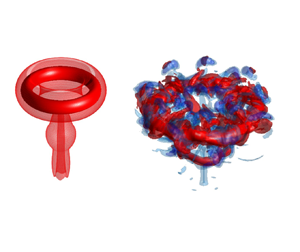
Figure 3 provides a comparison of the associated vortex structure at different times during the evolution of the flow for swirl numbers  ${S}=0$ and $1$, and inlet Case A; in which the leading, toroidally shaped primary ring is clearly identifiable together with the wake, or trailing jet. Figure 3(a) reveals that the primary ring core, when ${S}=0$, remains almost perfectly axisymmetric for the duration of the simulation, and the absence of any negative vorticity ( $\omega _\theta <0$) in that $\omega _\theta >0$ everywhere (denoted as red isosurfaces) – the opposite of what is observed in the remaining images, figures 3(b)–3(d) when $S=1$, and which display a number of distinguishing features. First, significant regions of negative vorticity (denoted as blue isosurfaces) are found to exist surrounding the main vortex core at the times shown, and is indeed found to be present from the outset. Second, the flow structure loses stability at large time, figure 3(d), manifesting as a wavy primary vortex core and a broken vortex structure in the azimuthal direction and featuring both positive and negative vorticity outside of the vortex core. At $T^*=12$, a secondary vortex ring can also be seen which rolls up at the downstream end of the trailing jet when discharge stops. As discussed later in § 3.6, the strength of this secondary ring depends on $S$, and has non-trivial impact on the growth of the leading ring circulation.

Figure 3. Vortex structure visualised, for swirl numbers  $S=0,1$ and inlet Case A, as isosurfaces of $\omega _{\theta }D_{o}/U_{o}=[\mathrm {levels:}-2.5, -1.25, 2.5, 5]$, with red and blue denoting positive and negative values of vorticity, respectively. (a) ${S}=0$ at $T^*=12$; (b) ${S}=1$ at $T^*=6$ (the moment the discharge stops); (c) ${S}=1$, $T^*=8$ and (d) ${S}=1$, $T^*=12$.
The amplitude of the wave along the vortex core can be estimated in terms of the degree of asymmetry of the core centroid, whose coordinates  $(R,Z)$ for a given $\theta$ plane can be obtained from
 \begin{equation} R(\theta)=\frac{\displaystyle\iint\omega_{\theta}(\theta)r\,\mathrm{d}r\,\mathrm{d}z}{\displaystyle\iint \omega_{\theta}(\theta)\,\mathrm{d}r\,\mathrm{d}z} \quad Z(\theta)=\frac{\displaystyle\iint\omega_{\theta}(\theta)z\,\mathrm{d}r\,\mathrm{d}z}{\displaystyle\iint \omega_{\theta}(\theta)\,\mathrm{d}r\,\mathrm{d}z}, \end{equation}
where regions in which  $\omega _\theta \geqslant \omega _\theta (\mathrm {max})e^{-1}$ in the primary vortex core are assumed to contribute; here, $\omega _\theta (\mathrm {max})$ is the maximum $\omega _\theta$ in the vortex core centre. Above this threshold magnitude, $\omega _\theta <0$ does not exist. Figure 4 examines the time evolution of the standard deviation, $\sigma _{R}$, of $R(\theta )$ for different representative swirl numbers and inlets Case A and B. Waviness is also reflected in the $Z(\theta )$ component, which is consistent. Note that the absolute ring radius $R$ increases rapidly over time as $S$ increases, as discussed in § 3.3, in particular for the case $T^{*}>6$ and $S\geqslant 3/4$.

Figure 4. Evolution of vortex core asymmetry, expressed in terms of the standard deviation,  $\sigma _{R}$, of $R(\theta )$ given by (3.1a,b) for different $S$ values and both inlets Case A and B.
The primary core in figure 3(d) exhibits a wavenumber for the azimuthal asymmetry of  $m=3$, which is determined by spectral analysis of $R(\theta )$ (figure not shown). The time dependence of the magnitude of the primary spectral peak also agrees well with that of $\sigma _R$. Accordingly, figure 4 reveals that for the Re under investigation, core waviness develops to a noticeable level for $T^*>8$, other than when $S=0$ with experiments showing that azimuthal waviness does not develop until after very large time (Maxworthy Reference Maxworthy1977). The corresponding temporal behaviour for $S=1$ and inlet Case B confirms that the loss of azimuthal symmetry is instability induced, which is not driven by the choice of inlet geometry. The amplitude of the waves, reflected by $\sigma _{R}$, increases with time as well as $S$. The azimuthal instability will eventually lead to turbulence and breakdown of the vortex core; before this occurs, the leading primary ring propagates downstream as a coherent structure – which is typically isolated and compact after it detaches from the trailing jet.
The dominant wavenumber  $m$ induced by instability depends nonlinearly on $S$, and could also be time dependent. However, it only becomes important at relatively large time (see the experiment of He et al. Reference He, Gan and Liu2020a). The present study considers small time only; that is, before core waves develop significantly. As such, for $T^*\leq 12$, axisymmetric flow is a reasonable assumption, permitting the process of azimuthal averaging to reflect the global behaviour of these flows in their axisymmetric $r\unicode{x2013}z$ planes.
3.2. Distribution of azimuthal vorticity  $\omega _\theta$

3.2.1. Regions of $\omega _\theta >0$

As the dominant vorticity component in a non-swirling vortex ring, regions of  $\omega _\theta >0$ in a swirling ring reflect a weak dependence on $S$. They mainly originate as a consequence of a $\omega _\theta$ flux from a modified boundary layer profile at an orifice exit, as in Case A. Figure 5(a) shows the dependence of the axial velocity $u_z$ on $r$ at the $z=0$ plane when $T^*=0.4$, which correctly replicates the Richardson's annular effect similarly observed in starting jets, where $u_z$ becomes a maximum ( ${\approx }1.2U_0$) at $r\approx 0.95R_o$ outside of the boundary layer and a minimum ( ${\lesssim }U_0$) at $r=0$ satisfying mass conservation (Didden Reference Didden1979; Lim & Nickels Reference Lim and Nickels1995). It also is related to the acceleration of $u_z$ close to the orifice edge induced by the rolled-up vortex core at earlier time, which increases the magnitude of $\partial u_z/\partial r$ and in turn that of $\omega _\theta$; see (2.8).

Figure 5. (a) Dependence of  $u_z$ on $r$ at $z=0$ (Case A); for Case B, $u_z=U_0$, and independent of $S$. (b) Dependence of $u_r$ on $r$ (Case A). (c) Dependence on $S$ of the total circulation flux $\partial \varGamma /\partial t$ at $z=0$ (Case A and B). (d) Dependence on $S$ of the total circulation components $\varGamma _{u_{r}}$, $\varGamma _{u_{z}}$ defined in (3.2) (Case A). The plots all correspond to $T^{*}=0.4$ and the direction of the arrow in (a,b) indicates increasing $S$.
$S$.
The flux of circulation associated with  $\omega _\theta$ through the orifice exit can be calculated, using (2.8), as
 \begin{align} \frac{\partial\varGamma}{\partial t}=\int_0^{R_o}\omega_\theta u_z\,\mathrm{d}r &=\int_0^{R_o}\left(\frac{\partial u_r}{\partial z}-\frac{\partial u_z}{\partial r}\right)u_z\,\mathrm{d}r \nonumber\\ &= {\underbrace{\int_0^{R_o}\frac{\partial u_r}{\partial z}u_z}_{\varGamma({u_{r}})}}\,\mathrm{d}r+ {\underbrace{\left.\frac{1}{2}u_z^2\right|_{r=0}}_{\varGamma({u_{z})}}}. \end{align}
The second term in (3.2) is related to the slug model and is only connected to  $u_z$ at the axis ( $r=0$), since $u_z=0$ at $r=R_o$. The dependence of $u_r$ on $r$ is shown in figure 5(b), where $u_r$ is clearly non-zero at $z=0$ owing to the velocity induced by the rolled-up vortex core (Didden Reference Didden1979). Nevertheless, it is an order of magnitude smaller than $u_z$. The total circulation flux $\partial \varGamma /\partial t$ through the orifice plane, shown in figure 5(c), reveals a weak dependence on $S$ for Case A only. Figure 5(d) further reveals the effect of $S$ on the production of $\partial \varGamma /\partial t$ for Case A. It can be seen also from (3.2) that adding swirl diminishes the contribution from $\varGamma (u_{z})$, but increases that from $\varGamma (u_{r})$. Although the contribution of $\varGamma (u_{r})$ can be significant if the $u_r$ profile is purposely manipulated (see e.g. Krieg & Mohseni Reference Krieg and Mohseni2013), the straight nozzle in Case A implies that it is moderate here.
For the idealised orifice, Case B, no surface is present for a boundary layer to develop, unlike Case A, and the  $u_z(r)$ profile is independent of $S$ at $z=0$ which is exactly the inlet plane. Therefore, no swirl induced $\omega _\theta$ flux effect exists, as evidenced in figure 5(c), where only the $\varGamma (u_z)$ term in (3.2) contributes. It is a constant for Case B and of similar magnitude to the same term for Case A. However, immediately outside the exit (e.g. at $z=0.1D_o$), the primary ring core introduces a $\varGamma (u_r)$ effect which results in a similar dependence on $S$, as shown in figure 5(d), rendering the overall $\partial \varGamma /\partial t$ similar to that of Case A.
Profiles of the kind provided in figure 5 ( $u_z$, $u_r$ and their associated circulation contributions $\varGamma (u_z)$, $\varGamma (u_r)$) are transient. Those shown in this figure are for $T^*=0.4$; a time when the primary ring is in the early stages of being formed and its location is very close to the orifice exit. The primary core imposes a strong influence on these quantities, which feeds back to the vorticity flux. This is a mutual process. When the leading ring propagates away (in both the $z$ and $r$ direction depending on $S$), its influence, especially the $\varGamma (u_r)$ component, fades as does $\partial \varGamma /\partial t$; hence, the growth of the total $\varGamma$ in the flow domain (discussed later in § 3.6), tends to be steady. Compared with that in Case A, the steady shear layer (or trailing jet) outside of the orifice exit in Case B is thinner in general owing to the absence of the boundary layer effect present in the former, which results in slightly smaller $\partial \varGamma /\partial t$ and, more importantly, is more prone to instability (Zhao, Frankel & Mongeau Reference Zhao, Frankel and Mongeau2000).
The overall effect also implies that the peak  $\omega _\theta$ in the vortex core centre is smaller for Case B than Case A and is less sensitive to $S$; for Case A, it increases weakly with $S$ at early formation time. This is supported by the findings shown in figure 6, even after the absolute peak vorticity is scaled by the instantaneous ring radius $R(t)$; the rationale for choosing this scaling parameter is discussed next.

Figure 6. Evolution of  $\omega _\theta ^*(\mathrm {max})$, the scaled peak vorticity in the ring core centre, for different $S$. The solid lines are fitting function $\omega _\theta ^*(\mathrm {max})\sim (T^*-T_0^*)^{-1}$, where $T_0^*=-1$ and $-1.37$ for Case A and B, respectively, are virtual time origins.
Soon after the vortex core is formed, roll-up of  $\omega _\theta$ in the vortex sheet from the orifice wraps around the outside of the core, leaving the core largely unaffected and remaining Gaussian like (Saffman Reference Saffman1995, Reference Saffman1975). In the absence of swirl and assuming the curvature of the toroidal core to be negligible (i.e. $R$ large), the distribution of $\omega _\theta (r,t)$ in the moving frame of reference centred at the core for an infinitely long vortex tube can be approximated by a Lamb–Oseen vortex (Saffman Reference Saffman1978; Weigand & Gharib Reference Weigand and Gharib1997; Fukumoto & Moffatt Reference Fukumoto and Moffatt2000), which is a solution of the generalised vorticity equation
 \begin{equation} \frac{\partial \omega}{\partial t}=\nu\left(\frac{\partial^2\omega}{\partial r^2}+\frac{1}{r}\frac{\partial \omega}{\partial r}\right). \end{equation}
With proper boundary and initial conditions, (3.3) leads to an exact solution of the form
 \begin{equation} \omega(r,t)=\frac{C}{4{\rm \pi}\nu t}\exp\left(-\frac{r^2}{4\nu t}\right)=\omega(0,t)\exp\left(-\frac{r^2}{r_c^2}\right), \end{equation}
where  $\omega (0,t)$ is the peak $\omega _\theta$ in the core centre. Here, a local coordinate system is adopted with $r=0$ at the centre of the vortex core, instead of the orifice geometry. The circulation of the vortex core $\varGamma _c$, which is related to the peak vorticity $\omega (0,t)$ via
 \begin{equation} \varGamma_c=\int_0^{r_c}2{\rm \pi}\omega(0,t)\exp\left(-\frac{r^2}{r_c^2}\right)r\,\mathrm{d} r={\rm \pi} r_c^2\left(1-e^{{-}1}\right)\omega(0,t), \end{equation}
is constant (due to the growth of  $r_c$ under viscous diffusion), verifiable via (3.4). Equations (3.5) and (A1) (see Appendix A) result in the following relationship:
 \begin{equation} \omega(0,t)\sim \frac{\varGamma_c}{r_c^2}\sim\frac{R(t)}{V(t)}\sim\frac{R(t)}{t}, \end{equation}
where  $V(t)$ is the time dependent volume of the toroidal core having radius $R(t)$ and the (circular) cross-sectional radius $r_c$.
The evolution of the scaled peak vorticity,  $\omega _\theta ^*$, in the ring core centre is then
 \begin{equation} \omega_\theta^*(\mathrm{max})=\left[\frac{\omega_\theta(0,t)}{R(t)}\right]\left(\frac{D_o^2}{U_0}\right)\sim\frac{1}{T^*}. \end{equation}
This relationship is demonstrated in figure 6 for inlet Case A and B. It can be seen from (3.6) that without vortex stretching (constant  $R$),
$R$),  $\omega (0,t)\sim t^{-1}$; in which case figure 6 essentially manifests the decay of $\omega _\theta (0,t)$ due to viscous diffusion, after the vortex stretching effect is scaled. It further suggests that the $R$ behaviour, i.e. the stretching of the toroidal vortex core, is an important influential factor induced by swirl on top of viscous diffusion. Figure 6 also reveals that the difference between the decay profiles of $\omega _\theta ^*(\mathrm {max})$ diminishes as $T^*$ increases, becoming almost indistinguishable once discharge terminates at $T^*=6$.
As for the overall circulation of the leading ring, the differing swirl strength does not impact the similarity of the  $\omega _\theta$ roll-up process in the core area during the formation process. This is confirmed by the almost universal Gaussian like $\omega _\theta$ distribution, regardless of $S$ or orifice geometry (as discussed in § 3.4). Nevertheless, swirl weakly affects the evolution of the leading ring circulation, as evidenced in figure 7, where $\varGamma ^*_{Ring}$ is the circulation of the leading ring normalised in accordance with (2.7). The algorithm used to produce this figure was designed specifically to isolate only the leading ring area, excluding the trailing jet which is not fully rolled into the ring core area. It shows that during discharge ( $T^*\leq 6$), the mechanism of $\omega _\theta$ delivery to the leading ring volume is fairly universal, with $\varGamma ^*_{Ring}$ increasing subtly with $S$ due to higher $\omega _\theta$ flux. For $T^*>6$, the behaviour of $\varGamma ^*_{Ring}$ for Case A and B begin to deviate from one another. With reference to figure 7(a), for $S=0$ and $1/4$, $\varGamma ^*_{Ring}$ continues to increase by ingesting vorticity ( $\omega _\theta >0$) from the trailing jet to the leading ring, whilst for $S \geqslant 1/2$, $\varGamma ^*_{Ring}$ increases until $T^*\gtrsim 8$, before decaying at a rate proportional to $S$. This is due to the stronger vorticity cancellation between the ring core ( $\omega _\theta >0$) and the peripheral region of $\omega _\theta <0$ (as discussed in § 3.2.2), which increases with $S$ and overwhelms the vorticity ingested from the trailing jet.

Figure 7. Evolution of the leading ring circulation  $\varGamma ^*_{Ring}$. (a) All $S$ (Case A); (b) comparison of Case A and B for $S=0$ and $1$.
$1$.
Figure 7(b) examines the impact of orifice geometry on the evolution of  $\varGamma ^*_{Ring}$. For clarification purpose, only $\mathrm {S}=0$ and $1$ are shown, the behaviour of other $S$ cases being consistent. In line with $\omega _\theta ^*(\mathrm {max})$ in figure 6, Case B displays an appreciably smaller $\varGamma ^*_{Ring}$ for the same $S$ owing essentially to the absent $\omega _\theta$ flux effect at the orifice exit illustrated in figure 5, but the overall dependence on $T^*$ is similar to that of Case A.
3.2.2. Regions of $\omega _\theta <0$

A striking consequence of the presence of swirl in the flow of interest is the generation of significant regions of  $\omega _\theta <0$ (negative vorticity) from the start of the formation process, as reported by Naitoh et al. (Reference Naitoh, Okura, Gotoh and Kato2014), Gargan-Shingles et al. (Reference Gargan-Shingles, Rudman and Ryan2015), Cheng et al. (Reference Cheng, Lou and Lim2010) and He et al. (Reference He, Gan and Liu2020b); although in the case of the latter, it is uncertain whether the negative vorticity originates from the boundary layer washed off the surface of the vanes creating the swirl velocity component. From figure 8(a), $S=1$ and inlet Case A, three distinct regions of $\omega _\theta <0$ can be identified. Region I stems from $\omega _\theta \sim \partial {u_r}/\partial {z}$ in the boundary layer developed by the inward flush of fluid induced by the circulation of the leading vortex core ( $\omega _\theta >0$); Region II issues from the orifice and is related to the imposed axial velocity profile, i.e. $\omega _{\theta }\sim -\partial {u_{z}}/\partial {r}$; Region III is the main contributor of $\omega _\theta <0$ and is formed ahead and in the proximity of the main vortex core (see also figure 3b), as observed in the above studies. Note that for inlet Case B, the intensity in Region II is much weaker than that in Case A, in accord with the $u_z$ profile imposed at the orifice exit; see figure 5(a).

Figure 8. (a)  $\omega _\theta$ contours for $S=1$ at $T^{*}=4$; Regions I, II and III indicate the presence of negative vorticity (Case A). Distribution of $\omega _\theta$ for Case B at the same $S$ and $T^{*}$ is very similar albeit the absence of Region II. (b) Dependence on time of the production rate of $\omega _\theta <0$ due to vortex tilting, for different $S$ (Case A). Symbol legend is the same as that for figure 7(a).
The magnitude of  $\omega _\theta$ in Regions I and II increases slightly with $S$; for the former, this is attributed to the increment of $\varGamma _{Ring}$ (figure 7), and hence the stronger $u_r$ induced on the vertical wall outside the orifice; for the latter, it is due to the slight increase of $\partial {u_z}/\partial {r}$ on the inner side of the jet at the orifice exit (figure 5a). They are both weaker than that in Region III, where $\omega _\theta ({<}0)$ is of the same order of magnitude as $\omega _\theta ({>}0)$ in the leading vortex ring core, as shown in figure 8(a).
Cheng et al. (Reference Cheng, Lou and Lim2010) attributes the formation of negative vorticity observed in their work to the secondary flow induced by  $u_\theta$ in the toroidal core, by a mechanism analogous to the secondary flow induced inside a curved pipe. In their study, this secondary flow is characterised by the formation of a vortex pair commonly known as Dean vortices, within which, positive vorticity feeds the primary vortex ring having the same vorticity sign, increasing its circulation; meanwhile, the negative vorticity interacts with the primary ring, forming complex vortex structures. A suitable dimensionless number that characterises this phenomenon is the Dean number ${De}$, the ratio of the product of centrifugal and inertia forces to the viscous force (Berger, Talbot & Yao Reference Berger, Talbot and Yao1983), given by
 \begin{align} {De}&=\displaystyle\left[\frac{2a(t) u_\theta(t)}{\nu}\right]\left[\frac{a(t)}{R(t)}\right]^{{1}/{2}} \nonumber\\ &=\displaystyle\left[\frac{2a(t)}{D_o}\right]^{{3}/{2}}\left[\frac{u_\theta(t)}{U_0}\right]\left[ \frac{D_o}{2R(t)}\right]^{\frac{1}{2}}{Re}, \end{align}
where, in the toroidal vortex core, both the radius  $r_c$ and swirl velocity $u_\theta (t)$ are time dependent, as well as the ring radius $R(t)$. The order of magnitude of the maximum ${De}$ for the cases investigated, viz. ${S}=1$, can be estimated, by taking $2a(t)\sim D_o/10$, $u_\theta \lesssim \varOmega R_o/2= U_0/2$ (as detailed in § 3.4), $D_o\lesssim 2R(t)$. It turns out that typically ${De}< 40$ (in the range of 20 to 55) for $0.4< T^{*}<6$, whilst for the swirling rings of Cheng et al. (Reference Cheng, Lou and Lim2010), $De \sim 640$, an order of magnitude greater. Note that the swirl component of Cheng et al. (Reference Cheng, Lou and Lim2010) was superposed onto a well-formed Gaussian ring and has a very different $u_\theta$ distribution in the ring core, which is discussed in § 3.4.
According to Berger et al. (Reference Berger, Talbot and Yao1983), secondary flow is induced at  $De>36$ and remains laminar until $De \approx 176$. On the one hand, a Dean vortex pair similar to that of Cheng et al. (Reference Cheng, Lou and Lim2010) is not observed in the present study; on the other, the intensity of the negative vorticity in their study is appreciably lower, albeit at a $De$ one order of magnitude larger. This suggests that when the swirl component is generated simultaneously with ring formation, some other mechanism dominates the generation of negative vorticity in Region III.
Inspired by the work of Brown & Lopez (Reference Brown and Lopez1990), Darmofal (Reference Darmofal1993) adopted a theoretical approach to explain that for a continuous swirling jet, negative vorticity originates from the tilting of  $\omega _z$, which eventually leads to vortex breakdown. It is an inviscid process. This can be seen from the $\omega _\theta$ component of the inviscid vorticity equation
 \begin{equation} \frac{{\rm D}\omega_\theta}{{\rm D}t}=\omega_{r}\frac{\partial{u_{\theta}}}{\partial{r}}+ \omega_{z}\frac{\partial{u_{\theta}}}{\partial{z}}+\frac{u_{r}\omega_{\theta}}{r}, \end{equation}
where  ${\rm D}/{\rm D}t$ is the standard material derivative in cylindrical polar coordinates and
 \begin{equation} \omega_{z}=\frac{1}{r}\frac{\partial{\left(ru_{\theta}\right)}}{\partial{r}}, \quad \omega_{r}={-}\frac{\partial{u_{\theta}}}{\partial{z}}. \end{equation}
The production of negative vorticity in Region III is postulated to originate from the tilting terms (the first two terms on the right-hand side of (3.9)); while the vortex stretching term (the last term) amplifies its intensity at a rate proportional to  $u_r$, as expected. For vortex rings without swirl, $u_\theta =0$, the contribution from vortex tilting is zero and therefore negative vorticity is never observed in Region III in this case. The production of negative vorticity from the tilting terms can be quantified by substituting (3.10a,b) into (3.9), resulting in
 \begin{equation} \left(\frac{\partial\omega_\theta}{\partial t}\right)_{T}=\frac{1}{2}\frac{\partial}{\partial{z}}\left(\frac{{u_{\theta}}^2}{r}\right), \end{equation}
the subscript ‘T’ on the left-hand side denoting vortex tilting. Since the term on the right-hand side, which is the gradient with respect to  $z$, is negative in the leading area and approximately coincides with Region III (figure not shown, but can be inferred from the $u_\theta$ distribution in the $r\unicode{x2013}z$ plane, as discussed in § 3.4), negative $\omega _\theta$ is generated there, regardless of the direction of $u_\theta$. According to the distribution of $\partial ({u_{\theta }}^2/r)/\partial {z}$ (figure not shown), strong tilting initiates on $r=0$ closer to the windward stagnation point in the moving frame (this is discussed further in § 3.3). Fluid having negative vorticity is then transported and stretched around the vortex core; $u_{\theta }$ inside the core does not contribute directly to the generation of negative vorticity. This supports the finding of Gargan-Shingles et al. (Reference Gargan-Shingles, Rudman and Ryan2015) that the gradients of $u_{\theta }$ are the source terms of the negative $\omega _\theta$. The rate at which the total circulation, $\varGamma _{T}$, is produced by vortex tilting can be obtained from
 \begin{equation} \frac{\partial{\varGamma_{T}}}{\partial{t}}=\int_A\left(\frac{\partial{\omega_\theta}}{\partial{t}}\right)_{T} \,\mathrm{d}A=\frac{\partial}{\partial{t}}\int_A \left(\omega_\theta\right)_{T}\,\mathrm{d}A= \frac{1}{2}\int_A\left[\frac{\partial}{\partial{z}}\left(\frac{{u_{\theta}}^2}{r}\right)\right]\mathrm{d}A, \end{equation}
where the constant integration area  $A$ is the same as that in (2.7), which is the entire flow domain. Figure 8(b) shows the change in $\partial \varGamma _{T}/\partial t$, over the discharge duration ( $0< T^*\leq 6$), calculated using (3.12) with the $u_\theta$ distribution over $A$; confirming that for $S=0$, no negative vorticity is generated due to zero $u_\theta$ everywhere. The rate of production of negative vorticity from vortex tilting appears to be constant for a given $S$ for $T^*>2$, and mainly contributed by Region III. It suggests that even though $u_\theta$ intensity in the vortex core decreases over time due to viscous diffusion (see § 3.4), the production rate is maintained, since the gradient with respect to $z$ is contributed to from the peripheral area of the core. The production rate is also a nonlinear function of $S$, as evidenced by the uneven spacing between the lines in figure 8(b).
Thus, the dependence of  $\varGamma _{T}$ on time can be evaluated as
 \begin{equation} \varGamma_{T}\left(t\right)= \frac{1}{2}\int_0^{t}\int_A\left[\frac{\partial}{\partial{z}}\left(\frac{{u_{\theta}}^2}{r}\right)\right] \mathrm{d}A\,\mathrm{d}t, \end{equation}
which suggests that  $\varGamma _{T}$ scales like
 \begin{equation} \varGamma_{T}\sim u_\theta^2\sim \left(SU_0\right)^2\sim S^2. \end{equation}
Figure 9(a) presents the time variation of the circulation associated with the negative vorticity in Regions II and III, excluding Region I. This circulation is denoted  $\varGamma (-)$, and calculated by integrating $\omega _\theta$ over the two Regions. It suggests that for $S\geqslant 1/2$, Region III (vortex tilting $\varGamma _{T}$) is the main source of negative vorticity generation, and $\varGamma (-)$ scales with $S^2$ according to (3.14). For $S=1/4$ and both inlet Case A and B, the main contribution to $\varGamma (-)$ is Region II, and therefore the scaling does not hold; for $S=1/4$ and Case B, the weaker $\partial u_z/\partial r$ diminishes the magnitude of $\varGamma (-)$ compared with that for Case A. Note that the stretching term in (3.9) does not contribute to the generation of $\varGamma (-)$ in an inviscid flow, according to Kelvin's circulation theorem.

Figure 9. (a) Time variation of  $\varGamma (-)$, the circulation associated with $\omega _{\theta }(<0)$ in regions II and III of figure 8(a). Inlet Case B, for $S>1/4$, shows behaviour consistent with that for Case A. Symbol legend is the same as that for figure 7(a). (b) Dependence on $S$ of the total circulation $\sum _t\varGamma (-)$ associated with $\omega _\theta <0$ in Regions II and III, integrated over $0< T^{*}\leq 6$, and that contributed by vortex tilting calculated via (3.13); although these results are for inlet Case A, those for inlet Case B show consistent behaviour, but are roughly $3\,\%$ higher for each $S$.
$S$.
In addition, figure 9(a) shows that the production of negative vorticity starts in tandem with the formation of the primary ring. Unlike the flow studied by Brown & Lopez (Reference Brown and Lopez1990) and Darmofal (Reference Darmofal1993), where vortex breakdown is caused by flow instability, for the vortex ring flow considered here, which is a starting swirling jet, the roll-up of the primary vortex core triggers the breakdown from  $t=0$. For any $S>0$, $u_\theta ^2>0$, and the $u_r$ induced by the primary core promotes the generation of negative $\omega _\theta$ by tilting $\omega _z$.
The total negative vorticity produced from vortex tilting during formation can also be calculated from (3.13) by setting the upper integration limit to  $T^*=6$, the total discharge time. The result is shown in figure 9(b) in terms of $S$ dependence. The variation of the total $\varGamma _T$ is consistent with that of $\varGamma (-)$, with the difference contributed by Region II, which in general increases appreciably with $S$.
$S$.
It is worth noting that Naitoh et al. (Reference Naitoh, Okura, Gotoh and Kato2014) reported low intensity negative vorticity in Region III, which dissipates quickly without much interaction with the primary ring structure where  $\omega _\theta >0$. The important difference in their flow field is the low piston stroke ratio of $L/D<2$, where almost all the vorticity flux through the nozzle exit was able to be entrained into the primary ring volume. Small $L/D$ gives rise to a reduced circulation of the primary ring, and subsequently diminishes the negative vorticity production rate by weakening vortex tilting (as discussed further in § 3.3). Thus, it can be argued that the formation of regions of $\omega _\theta <0$ is related more to the vortex tilting mechanism triggered by the swirling primary vortex ring structure.
3.3. Growth of the primary ring radius $R$

In figure 10(a), the dependence of the trajectory of the vortex's centroid on  $S$, calculated via (3.1a,b) for inlet Case B, is compared; the background image shown is the $\omega _{\theta }$ contour for $S=0$ at $T^*=8$. It reveals an unequivocal incremental trend for the ring radius $R$ in the $r$-direction, accompanied by a strong decrease of the ring core penetration distance in the $z$-direction as $S$ increases. This is in agreement with the experimental findings of He et al. (Reference He, Gan and Liu2020b) for a similar inlet condition, although at a $Re$ an order of magnitude higher and swirl not strictly of solid-body rotation type. For $S\leq 1/2$, trajectory dependence on $S$ appears to be weak; for $S>1/2$, this dependence becomes clearly stronger and seems to have a more-or-less linear dependence (equal spacing) on $S$. For inlet Case A, similar trajectories and contour plots arise, with a clear secondary ring arising in the wake for $S>0$; unlike Case B, no secondary ring is present when $S=0$.

Figure 10. (a) Swirl number specific vortex core centroid trajectories for  $T^*\leq 8$ (Case B); shown also is the $\omega _{\theta }$ contour plot associated with $S=0$ at $T^*=8$. (b) Evolution of the ring radius $R$ (Case A); the solid line is the fitting function $R\sim (T^*)^{1/4}$ for $S=0$. The direction of the arrow in (b) indicates increasing $S$. Symbol legend is the same as that for figure 7(a).
In previous studies, growth of the ring radius in the presence of swirl has commonly been attributed to the centrifugal force associated with  $u_\theta$ in the core but has not been discussed in any detail. In the work of Virk et al. (Reference Virk, Melander and Hussain1994), where $u_\theta$ peaks in the ring core, the ring growth rate is much smaller ( ${\approx }4\,\%$); since the swirl in their work is parametrised according to the degree of polarisation, it is difficult to directly compare their swirl intensity with that of the present work. The isolated Gaussian ring prior to the superposition of $u_\theta$ can effectively be considered as being formed after a sufficiently small discharge time. Alternatively, in the experimental study by Naitoh et al. (Reference Naitoh, Okura, Gotoh and Kato2014), for a similar physical formation process, the growth rates of $R$ for similar $S$ values are also smaller. This discrepancy is likely a result of the smaller discharge ratio, which was $L/D=2$, compared to the value $6$ in the present study. It suggests that whilst the centrifugal effect is indubitably responsible for the radial growth of an isolated and well-formed swirling ring, it is not the dominant factor during the vortex roll-up process, not least for long discharge times.
In figure 10(a), a secondary ring is seen to be forming at the far end of the trailing jet, as highlighted; see also figure 3(d). Typically, one (sometimes two) secondary ring(s) can be observed to form just after discharge terminates, due to shear layer instability, but they should not be confused with a stopping vortex having the opposite sign to the leading ring. Their characteristics depend strongly on  $S$. The only exception is for $S=0$ and Case A, where no clear secondary ring is seen. This is because this case has the most stable shear layer of all the cases under investigation; it has zero swirl and its shear layer is also thicker than for $S=0$ and inlet Case B, as mentioned in § 3.2.
For inlet Case A, figure 10(b) shows that for a ring without swirl,  $S=0$, the behaviour of $R$ can evidently be described by a power law in $T^*$, viz. $R\sim (T^*)^\beta$ with $\beta \approx 1/4$. It stems from dimensional analysis by considering the conservation of the specific hydrodynamic impulse, $I$, of the isolated leading ring when $S=0$ at high $Re$ where viscous effects are unimportant (Glezer & Coles Reference Glezer and Coles1990; Gan & Nickels Reference Gan and Nickels2010):
 \begin{equation} R(t)\sim \left(t-t_0\right)^{{1}/{4}}\left(I\right)^{{1}/{4}}, \end{equation}
where  $t_0$ is some virtual time origin to account for the orifice radius $R_o$. By neglecting the effect of added mass and the trailing jet,
 \begin{equation} I=\tfrac{1}{2}\int_{V}\boldsymbol{x}\times\boldsymbol{\omega}\,\mathrm{d}V\approx{\rm \pi} \int_{A_c}r^2\omega_\theta\,\mathrm{d}A, \end{equation}
which is unidirectional in  $z$. Here, $A_c$ represents the toroidal core sectional area. The small discrepancy between the fitted line and the data points in figure 10(b) can be attributed to the effect of the trailing jet as well as the moderate Re. For $S>0$, no reasonable corresponding power law relation is found due to a nonlinear mechanism associated with swirl, which is discussed below.
Figures 11(a) and 11(b) compare  $\omega _\theta$ contour plots when $S=0$ and $1$ for inlet Case A, together with instantaneous in-plane streamlines in the moving frame of reference travelling at the instantaneous propagation velocity of the leading primary vortex ring, $u_z'$, in the axial, $z$-direction (this is discussed further in § 3.5). The stagnation point, denoted as sp, is determined to lie at the axial position where $u_{z}=0$ at $r=0$ in this moving frame. For $S=0$, figure 11(a) shows the primary vortex core essentially moves in the axial direction with the radial velocity of the core $u_{r}'\ll u_{z}'$. The primary vortex is surrounded by the classical-shaped bubble (with wake) as revealed by the streamlines. The stagnation point is always located upstream of the vortex core, as shown in figure 11(c), with $Z_{sp}$, the difference between the $z$ coordinate of sp and that of the vortex core centroid, slowly increasing with time. This reflects the growth of the ring bubble volume due to entrainment of surrounding ambient fluid into the bubble (Gan & Nickels Reference Gan and Nickels2010). Although not shown, similar behaviour is observed for $S=1/4$ and $1/2$.

Figure 11. Instantaneous  $\omega _\theta$ contour plots at $T^{*}=6.4$ for (a) $S=0$, (b) $S=1$ (Case A); the overlaid dashed lines are the in-plane instantaneous streamlines in the frame of reference moving at the instantaneous $u_z'$. Here, sp indicates the location of the stagnation point on $r=0$ in this moving frame, and $Z_{sp}$ is the distance between sp and the vortex core centroid. (c) Dependence of $Z_{sp}$ on time (Case A); the corresponding dashed lines shown are for Case B and $S=0$ and $1$ only, since the remaining $S$ cases follow a pattern consistent with Case A. Symbol legend is the same as that for figure 7(a).
In contrast, for  $S=1$, figure 11(b) shows the vortex bubble breaks down as if the ring is about to pass over a (moving) bluff body. The relative position of the stagnation point, as shown in figure 11(c), suggests that initially at $T^*=0.8$, the shape of the bubble is similar for all the $S$ cases, but for $S\geqslant 3/4$, the stagnation point gradually moves towards the primary core, passing through ( $Z_{sp}=0$) at $T^*\approx 4$ and $5.6$, when $S=1$ and $7/8$, respectively. This upstream translation (in the moving frame) implies a deceleration of $u_z$ at $r=0$ around the stagnation point, which, in turn, accelerates $u_r$ as a consequence of satisfying continuity, similar to the breakdown mechanism in a continuous swirling jet (Darmofal Reference Darmofal1993; Billant et al. Reference Billant, Chomaz and Huerre1998). This is associated with the formation of the $\omega _\theta <0$ region, as can be clearly observed in figure 11(b) echoing figure 8(a), and can be interpreted via the Biot–Savart law (Brown & Lopez Reference Brown and Lopez1990)
 \begin{equation} u_{z}\left (0,z\right) =\frac{1}{2} \int\limits_{-\infty}^{\infty} \int\limits_{0}^{\infty}\frac{r^{2}\omega_\theta}{\left[r^{2}+(z-\acute{z})^{2}\right]^{3/2}}\, \mathrm{d}r\,\mathrm{d}\acute{z}. \end{equation}
That is, regions of  $\omega _\theta <0$ must be responsible for the deceleration of $u_z$ near the stagnation point and hence the behaviour change of $Z_{sp}$ with $S$. The $S$ dependent accelerated $u_r$, induced by the primary vortex core in the present case, further promotes the generation of negative vorticity, creating a nonlinear feedback for it (Darmofal Reference Darmofal1993), as well as for the behaviour of $R$ in figure 10(b) and the downstream movement of the stagnation point in figure 11(b). This complex mechanism explains the difficulty in identifying a single working scaling law for $R$ and all $S$.
$S$.
Likewise, figure 11(c) also shows that the behaviour of  $Z_{sp}$ varies nonlinearly as a function of $S$, showing an abrupt change between $S=1/2$ and $3/4$, suggesting the existence of a critical (or minimum) swirl number $1/2\lesssim \mathrm {S}_c<3/4$ for breakdown to occur. Finding this critical $S_c$ is left as a topic for future investigation.
3.4. Distribution of azimuthal velocity $u_\theta$

In previous numerical studies (Cheng et al. Reference Cheng, Lou and Lim2010; Hattori, Blanco-Rodríguez & Le Dizès Reference Hattori, Blanco-Rodríguez and Le Dizès2019), swirl was superposed onto a well-formed circular Gaussian vortex ring (in terms of the  $\omega _\theta$ distribution) as an axisymmetric and Gaussian distributed $u_\theta (r)$, with maximum intensity at the core centre. However, in practice, such a distribution of $u_\theta$ is hard to realise, if indeed possible; instead, it is more practical to introduce it via the roll-up process of the swirling vortex sheet in inlet geometries like Case A and B, as demonstrated in figure 12(a) which shows the swirling fluid material in the vortex core region appears to be diluted by engulfing the non-swirling ambient fluid at this early roll-up stage. The weaker $u_\theta$ in the core centre for Case A can plausibly be attributed to the roll-up of the non-swirling fluid in the short $0.1D_o$ long nozzle section (see figure 1) at the beginning of the formation process, which is equivalent to $T^* \in (0, 0.1]$.

Figure 12. (a) Contour plot of the magnitude of  $u_\theta$ in the $r$–
$r$– $z$ plane for $S=1$ at $T^{*}=0.8$ (Case A and B): the vertical dashed lines shown pass through the vortex core centroid based on $\omega _\theta$ (point $P_{2}$), determined by (3.1a,b); point $P_{1}$ marks the maximum $u_\theta$ along the dashed lines. (b) Distribution of $u_\theta$ and $\omega _\theta$ along the dashed lines in (a). (c,d) Variation of $u_\theta (r)$ distribution, at different times, in the core area (Case A and B), where $r_c$ is the local radial coordinate with $r_c=0$ at the core centroid; $a$ is the time dependent characteristic core radius, as defined in § 3.6.
The distribution of  $u_\theta (r)$ through the vortex core centre is plotted in figure 12(b) together with the distribution of $\omega _\theta (r)$. The vortex core can clearly be identified as the classical Gaussian like $\omega _\theta$ distribution centred at $r\approx 0.6D_o$ for both inlet Case A and B. It can be observed that at the core centre where $\omega _\theta$ peaks, the magnitude of $u_\theta$ is only approximately $1/5$ and $1/2$ of the maximum input swirl velocity $\varOmega R_o$, or $SU_0$, for Case A and B, respectively. This is approximately a local minima, instead of a local maxima. The peripheral region at $r\approx 0.55D_o$ and $0.7D_o$, having larger $u_\theta$, is the trace of the rolled-up layer from the edge of the orifice (see figure 12a), which does not diffuse towards the core centre in an efficient manner to make it Gaussian even over the entire scrutinised duration. In contrast, the viscous diffusion leads to a more homogeneously distributed $u_\theta (r)$ in the core area for both cases, diminishing their initial inhomogeneity. This is illustrated in figures 12(c) and 12(d), where the time dependence of the $u_\theta$ distribution in the core is presented. By $T^*\approx 4$, approximate homogenisation is reached and the geometrical dependence fades out thereafter in a manner of similarity. The local minima at $r_{c}/a\approx 1.8$, separating the shear layer and the core area, also appears to persist.
In figure 12(b), the inner shear layer can also be seen as a second  $\omega _\theta$ peak centred at $r\approx 0.5D_o$, aligned with the orifice edge. The $\omega _\theta$ intensity of the second peak for Case A is also larger, in line with the primary peak. The shear layer associated with $u_\theta$ is also consistent with this second peak. This is reflected by an almost linearly rapid drop of $u_\theta$ over the range $0.45D_o\lesssim r \lesssim 0.53D_o$, at almost the same rate for both orifice geometries. For $r\lesssim 0.45D_o$, $\omega _\theta \approx 0$ and solid-body rotation manifests in both cases as a constant gradient $\partial {u_\theta }/\partial r$, with that of Case B appreciably larger as expected.
The typical  $\omega _\theta$ distribution shown in figure 12(b) largely replicates that of a non-swirling vortex ring with a Gaussian core during formation (figure not shown), which suggests that introducing swirl does not significantly alter the similar $\omega _\theta$ distribution in the core area, and hence the fundamental roll-up process. However, different orifice geometries do have a clear impact on the peak $\omega _\theta$. That is, whilst Case B results in stronger $u_\theta$ in the vortex core, $\omega _\theta$ there is weaker, as also shown in figure 6.
Figure 13 presents the evolution of the averaged swirl intensity  $\overline {u_\theta }$ over the core area where $\omega _\theta \geqslant \omega _\theta (\max )e^{-1}$. A key feature is the dependence of $\overline {u_\theta }$ on orifice geometry. Owing to the discharge of an initially non-swirling fluid volume contained within the short $0.1D_o$ nozzle section, the maximum $\overline {u_\theta }$ attainable in the core centre for Case A is ${\approx }0.35\varOmega R_o$. In the absence of such a non-swirling volume, the maximum $\overline {u_\theta }$ in Case B is ${\approx }0.5\varOmega R_o$. The non-swirling volume in Case A also leads to a gentle increment of $\overline {u_\theta }$ but of short duration (for $T^*\lesssim 1.2$) before decay starts, whilst Case B displays a monotonic decay of $\overline {u_\theta }$ in the core centre. The difference between the $\overline {u_\theta }$ intensity as well as its decay rate for the two geometries becomes fairly small after discharge terminates at $T^*=6$. Comparing the dependence of $\overline {u_\theta }$ on $S$, it is clear that stronger swirl has lower resistance against $\overline {u_\theta }$ decay, for both inlet geometries. The decay of $\overline {u_\theta }$ can be well described by an exponential function of the form
 \begin{equation} \frac{\overline{u_\theta}}{SU_0}\sim C_1\exp({-}C_2 T^*)+C_3, \end{equation}
where  $C_1,C_2$ and $C_3$ are coefficients which are obviously $S$ dependent even after the scaling factor $S$ is incorporated. The exponential decay originates from viscous diffusion of $u_\theta$ in the core area, which is consistent with the form of (B2) derived from a diffusion model; see Appendix B.

Figure 13. Spatially averaged azimuthal velocity  $\overline {u_\theta }$ in the core area for (a) Case A, (b) Case B; the solid lines are fitting functions for $S=1$ of the form of (3.18). (c) Dependence of $u_\theta ^*$ on $T^*$ scaled as per (3.19); the fitting lines follow (3.20). The direction of the arrow in (b) indicates increasing $S$.
$S$.
Naitoh et al. (Reference Naitoh, Okura, Gotoh and Kato2014) suggests that the decay of  $u_\theta$ in the vortex core is attributable to the exchange of fluid between the ring and the ambient non-swirling fluid, the rate of which increases with $S$. Even though this effect could play an important role, it appears that $u_\theta$ behaviour is related to the combined effect of viscous diffusion (as shown) and the increment of ring radius $R$. As the initially irrotational free vortex flow outside a vortex undergoing solid-body rotation, which in this case is the jet rotating in the $r$–
$r$– $\theta$ plane issuing from the orifice, is similar to a Rankine vortex albeit of a finite length and influenced by the primary vortex roll-up, $\overline {u_\theta }$ in the ring core approximately decreases as $R^{-1}$ at a given time. Accordingly, a dimensionless swirl velocity $u_\theta ^*$ can be defined as
 \begin{equation} u_{\theta}^*=\frac{\overline{u_{\theta}}R(t)}{\varOmega R_{o}^2}= \frac{\overline{u_{\theta}}R(t)}{{S}U_0 R_{o}}. \end{equation}
 The dependence of  $u_\theta ^*$ on $T^*$ is shown in figure 13(c). The effectiveness of the scaling factor $R(t)$ is clear as it removes the effect of $S$ for a given orifice geometry, which is a dominant factor for the early time evolution of $u_\theta ^*$. The decay rate of $u_\theta ^*$ becomes almost geometrically independent after discharge terminates at $T^*=6$. Taking (3.15) and (3.18), the time dependence of $u_\theta ^*$ can well be described by
 \begin{equation} u_\theta^* \sim (T^*)^\beta[\exp(-\kappa T^*)+\mathcal{F}], \end{equation}
which is  $S$ independent. For the fitting lines shown in figure 13(c), $\beta$ takes a universal value of $1/4$, which seems to be attributed to the constant $I$ in the $z$ direction applied to all the cases tested. The fact that $\kappa =1/4$ ( $=\beta$, which could be a coincidence) suggests that the $u_\theta$ diffusion rate depends only weakly on the inlet orifice geometry. Here, $\mathcal {F}$, representing the behaviour of the initial roll-up of $u_\theta$ into the core area, see (B2), is apparently geometrically dependent, with a value $0.16$ and $0.22$ for inlet Case A and B, respectively. In general, the power law term in (3.20) dominates at early time, $T^*\lesssim 4$, with the exponential term dominating subsequently.
Physically, the scaling of (3.19) simply confirms that the strength (circulation) of the Rankine vortex mentioned above is proportional to  $S$, as expected, and the decay of this circulation becomes asymptotically similar for the two orifices, following the specified function of time in (3.20).
The behaviour of the time dependent (specific) angular momentum  $L(t)$ of the toroidal vortex core can also be inferred from (3.19), which can be written as
 \begin{equation} L=\int_{V}\boldsymbol{x}\times\boldsymbol{u}\,\mathrm{d}V\sim V(t)R(t)\overline{u_\theta}(t)\sim f(t,{S}), \end{equation}
where  $V(t)$ is the volume of the toroidal vortex core at time $t$ and $f(t,{S})$ denotes some function describing the evolution of $L$. It is not difficult to see that
 \begin{equation} L(T^*)\sim S(T^*)^{\beta+1}[\exp(-\kappa T^*)+\mathcal{F}]; \end{equation}
this is detailed in Appendix A. It can be deduced that for the range plotted in figure 13,  $L$ remains an increasing function of $T^*$, and increases according to viscous diffusion; i.e. the vortex ring entrains $u_\theta$ from the shear layer to the peripheral area around the core, which then diffuses towards the core centre. For $T^*\gg 9$, entrainment of $u_\theta$ from the shear layer terminates, and the decay rate of $u_\theta ^*$ is much greater and becomes ${S}$ dependent. This later stage is governed by viscous dissipation (figure not shown).
3.5. Propagation velocity $u_{z}'$ of the primary vortex ring

The leading primary ring structure propagates downstream as a compact coherent structure soon after the vorticity delivered by the shear layer outside the inlet orifice rolls up forming the vortex core. The magnitude of the propagation velocity is influenced by the self-induced velocity of the toroidal core, the shear layer in the trailing jet, as well as the swirl component. The dependence of this propagation velocity in the axial direction,  $u_{z}'$, on both time and swirl strength is presented in figure 14; $u_{z}'$ is calculated based on the azimuthal average of the core centroid $z$-coordinate as in (3.1a,b).

Figure 14. Leading vortex ring propagation velocity in the axial direction,  $u_{z}'$. Symbols denote inlet Case A and dotted lines Case B. The direction of the arrow indicates increasing $S$.
$S$.
Evidently, additional swirl decreases  $u_{z}'$, which is supported by previous numerical and experimental studies (Virk et al. Reference Virk, Melander and Hussain1994; Naitoh et al. Reference Naitoh, Okura, Gotoh and Kato2014; He et al. Reference He, Gan and Liu2020b). The effect of $S$ is weak at small time but gradually becomes more pronounced. The effect also appears to be stronger for larger $S$, i.e. $u_{z}'(S=0)\approx u_{z}'(S=1/4)\gg u_{z}'(S>1/2)$; $u_{z}'(S=0)\approx 2.35u_{z}'(S=1)$. For ${S} \leq 1/2$, despite the different absolute magnitude, the dependence of $u_{z}'$ on $T^*$ appears similar to that of a vortex ring without swirl. That is, $u_{z}'$ tends to a constant maximum value, before pinch-off, as a monotonic function. For $S\geqslant 3/4$, the behaviour of $u_{z}'$ changes appreciably. For example, $u_{z}'$ for $S=3/4$ is a maximum at $T^*\approx 3$, and then decreases to a stabilised value at $T^*\gtrsim 6$ when discharge terminates. For $S=7/8$ and $1$, additional complexity of $u_{z}'$ behaviour after $T^*=6$ is displayed; this is related to the influence of the stronger secondary ring after discharge ends, as shown in figure 10(a).
Comparing the overall behaviour of  $u_{z}'$ for Case A and B, it is evident that except for very early time, $T^*\lesssim 1$, the values obtained for Case A are consistently larger than for Case B. Their difference, $\Delta u_{z}'$, is relatively small for $S \leq 1/2$, but greatly increases as $S$ becomes larger. Dependence of $\Delta u_{z}'$ on $T^*$ also appears to be more complex for large $S$. Plausibly, this is owing to the nonlinear influence on $S$ of the $\omega _\theta$ flux, viz. $\partial \varGamma /\partial t$, leading to a larger $\varGamma _{Ring}$ (see figure 7) and hence $u_{z}'$ in Case A, as well as the more unstable shear layer of the trailing jet in Case B.
Saffman (Reference Saffman1995) provided a comprehensive model of  $u_{z}'$ for an isolated and perfectly circular thin core ring with swirl, which can be written as
 \begin{equation} u_{z}'=\frac{\varGamma_{Ring}}{4{\rm \pi}{R}}\left[\; {\underbrace{\ln\left(\frac{8}{\epsilon}\right)}_{T_1}}-0.5 +\underbrace{\frac{1}{\varGamma_{Ring}^{2}} \int_{0}^{a}\frac{\gamma^2(r)}{r}\,\mathrm{d}r}_{T_2}- \underbrace{\frac{8{\rm \pi}}{\varGamma_{Ring}^{2}}\int_{0}^{a}u_\theta^2r\,\mathrm{d}r}_{T_3}\;\right]+f(w), \end{equation}
where  $\epsilon =a/R$ is the ratio of the core radius $a$ (which is discussed again in § 3.6) to the ring radius $R$ calculated via (3.1a,b). Term $T_1$ is the canonical estimation of $u_{z}'$ for a (thin-cored) vortex ring without swirl, which is proportional to the leading ring circulation $\varGamma _{Ring}$; term $T_2$ is the additional correction factor which involves the detailed distribution of $\omega _\theta$ in the core, viz.
 \begin{equation} \gamma(r)=2{\rm \pi}\int_0^rr\omega_\theta(r)\,\mathrm{d}r \quad \textrm{where } \gamma(a)=\varGamma_{Ring}. \end{equation}
In the above equation, and in terms  $T_2, T_3$ of (3.23), a local coordinate system is applied such that $r=0$ is at the vortex core centroid and a perfectly circular core cross-section is assumed. Term $T_3$ quantifies the contribution from the azimuthal flow $u_\theta$. The last term $f(w)$ accounts for the effect of the trailing jet and the regions of $\omega _\theta <0$, which are not included in Saffman's model.
Equation (3.23) shows that if  $f(w)$ is neglected, for a given $\varGamma _{Ring}$ and $R$, introducing $u_\theta$ slows down $u_z'$. Based on a force-balance argument, Saffman (Reference Saffman1995) suggests that this is related to the balance between the centrifugal force generated by $u_\theta$ and the Kutta lift associated with the translational velocity $u_z'$. Therefore, to preserve the force balance, the Kutta lift has to decrease with the additional $u_\theta$ and consequently the propagation velocity $u_z'$ of the ring. The effect of swirl induced vortex tilting and breakdown further complicates matters.
The contribution from each of the three terms in (3.23) is evaluated and presented in figure 15, which unequivocally shows that  $T_1$ dominates the other two, regardless of $S$. The direct influence of $T_3$, which is associated with $u_\theta$ generated by the mechanism in this study, is one order of magnitude smaller. Its contribution is indirectly reflected by $R$, and hence $\epsilon$ in $T_1$, as well as the common factor $\varGamma _{Ring}/(4{\rm \pi} R)$. In this respect, the detailed $\gamma (r)$ distribution in (3.24) is least important. Figure 15(a) also suggests that the contribution when $S=1$ to $T_1$ is larger than when $S=0$, owing to smaller $\epsilon$, but the overall $u_z'$ is significantly smaller, as demonstrated in figure 14, because of the smaller common factor. It shows that the radius of the leading ring $R$ is the key parameter determining $u_z'$. Figure 15(b) demonstrates that $T_3(A)< T_3(B)$, in line with the findings for the spatially averaged $u_\theta$ in the vortex core discussed in § 3.4. Influence from both diminishes, as $u_\theta$ decays under viscous diffusion.

Figure 15. (a) Comparison of the relative contribution,  $T_{n}$, to $u_{z}'$ from the three terms in (3.23) for $S=1$, where (A) and (B) denote inlet Case A and B, respectively. The shades of grey increase from $T_1$ to $T_3$, $T_1$ being the lightest shade. The area under the dashed line in (a) is for the $T_1$ term for the case $S=0$. (b) Magnified view of the area in (a), represented by the dashed box in the bottom left-hand corner.
3.6. Formation process of the leading ring
Determination of the formation number  $F$, according to the definition of Gharib et al. (Reference Gharib, Rambod and Shariff1998), is illustrated in figure 16(a), which is the value of $T^{*}$ when the total circulation $\varGamma$ delivered by the orifice attains the maximum possible circulation of the leading ring, $\varGamma _{Ring}$, following pinch-off. Despite the three-dimensional nature of the flow, i.e. the instantaneous streamlines around the vortex core are of helical type owing to the swirling component, and discharge time also impacts on the detailed formation process as discussed by Limbourg & Nedić (Reference Limbourg and Nedić2021), here the classical circulation based formation number evaluated in the $r$–
$r$– $z$ plane is investigated, since the enstrophy of the flow is dominated by $\omega _\theta$. However, only $\omega _\theta >0$ is included when calculating the circulation for both the total domain and the leading ring $\varGamma _{Ring}$. As demonstrated in § 3.2.2, regions of $\omega _\theta <0$ originate from the tilting of $\omega _z$ (the swirl component). It is not produced by the inlet orifice directly, and its influence is taken into account in terms of interaction and cross-cancellation with the region of $\omega _\theta >0$. As $S$ increases, the contribution from the negative vorticity becomes significant as shown in figure 9. For comparison purposes, the total circulation is calculated, including $\omega _\theta <0$, and also displayed for $S=1$; including the negative vorticity leads to the total circulation dropping to zero at $T^*=8$ when the leading ring just gains maximum positive $\omega _\theta$. For $S=0$, the total circulation is largely unaffected in the absence of $\omega _\theta <0$ production.

Figure 16. (a) Determination of the formation number  $F$ based on the variation of the total, $\varGamma _{Total}$, and the leading ring, $\varGamma _{Ring}$, circulation with $T^*$ for inlet Case A. The leading ring circulation value $\varGamma _{Ring}$ is taken from figure 7(b). Symbols are for $\varGamma$ calculated from positive $\omega _\theta$ (with a small threshold) only; dashed lines represent $\varGamma$ obtained without applying a threshold (including $\omega _\theta <0$). (b) Dependence of formation number on swirl number $S$.
$S$.  ${\diamondsuit }$ $F(H)$, ${\bigcirc }$ $F(A)$, ${\Box }$ $F(B)$, where $k=\mathrm {d}F/\mathrm {d}S$. ( $A$), ( $B$) and ( $H$) signify Case A, Case B, and He et al. (Reference He, Gan and Liu2020b), respectively.
The total circulation in figure 16(a) shows that even though the  $\varGamma$ flux at the orifice exit increases with $S$, see (3.2), cancellation of positive and negative vorticity leads to a similar growth rate for the different $S$ cases, especially at early time. Also because of such cancellation, the growth rate of the total circulation when $S=1$ decreases, unlike that for $S=0$ where the growth rate remains constant in accordance with the constant $\omega _\theta$ flux at the orifice exit. The total circulation maximises when the discharge terminates at $T^*=6$, as expected. After that, the total circulation when $S=1$ decreases dramatically because of cancellation by the strong negative vorticity, but $\varGamma _{Ring}$ continues to grow until $T^*\approx 8$. The dependence of $F$ on $S$ is essentially determined by the maximum $\varGamma _{Ring}$ alone, which is detailed in § 3.2.1, because of the insensitivity of $S$ to the total circulation magnitude.
The  $F$ determined in this way is presented in figure 16(b) for Case A and B, together with the experimental results of He et al. (Reference He, Gan and Liu2020b). For $S=0$, $F\approx 3$, which is similar to the simulation result of Rosenfeld et al. (Reference Rosenfeld, Rambod and Gharib1998). The values of $F$ in the experiment of He et al. (Reference He, Gan and Liu2020b) are smaller but in a consistent way at a given $S$, plausibly owing to the higher turbulence levels introduced by the swirl-generating vanes and the slightly different ways of determining $F$. Figure 16(b) reflects a remarkably similar linear relation between the behaviour of (the circulation-based) $F$ with $S$, excluding and offset by the value at $S=0$. It is insensitive to Re, turbulence level and the detailed $u_\theta$ distribution in the vortex core from a practical swirl generation mechanism. In particular, the two orifice geometries result in very similar gradients, $k$.
$k$.
A second method proposed by Gharib et al. (Reference Gharib, Rambod and Shariff1998) for the determination of  $F$ uses the generic dimensionless kinetic energy $\alpha$ defined as
 \begin{equation} \alpha=\frac{E}{\sqrt{\rho{I}{\varGamma}^{3}}}, \end{equation}
where  $\varGamma$ and $I$ are calculated from (2.7) and (3.16), respectively. In energy terms, pinch-off occurs when $\alpha$ delivered by the nozzle (decreases with time) drops to the asymptotic value of an isolated ring $\alpha _{r}$. For rings with $S=0$, the leading ring reaches an asymptotic status at $T^*\approx 12$, as shown in figures 7 and 16(a). This occurs when the leading ring pinches-off from its trailing jet, and the corresponding limiting energy for the leading ring is $\alpha _r\approx 0.33$. As swirl $u_\theta$ induces $\omega _\theta <0$ for the $S>0$ cases, no asymptotic status is reached, due to vorticity cancellation. Approximating the ring as a member of the Norbury–Fraenkel family (Fraenkel Reference Fraenkel1972; Norbury Reference Norbury1973), Shusser & Gharib (Reference Shusser and Gharib2000) proposed an expression for $\alpha _{r}$ as a function of a single parameter $\epsilon$, defined as the ratio of core radius $a$ to ring radius $R$, such that
 \begin{equation} \alpha_r=\frac{\ln\displaystyle\left(\frac{8}{\epsilon}\right)-\frac{7}{4}+\frac{3}{8}{\epsilon}^2\ln\left(\frac{8}{\epsilon}\right)}{2\sqrt{{\rm \pi}\left(1+\displaystyle\frac{3}{4}{\epsilon}^2\right)}}. \end{equation}
The core radius  $a$ is taken as the equivalent radius for an area of $\omega _{\theta }\geqslant \omega _{\theta }(\max )e^{-2}$, and $\epsilon =a/R$ is plotted in figure 17(a). As discussed above, the consequence of adding swirl is reflected in the $r$–
$r$– $z$ plane in the promotion of ring radius growth. This tends to reduce $a$ because of the stretching of the vortex core, which in turn significantly reduces $\epsilon$. In comparison, the slow incremental change of $\epsilon$ for $S=0$ is the result of (viscous) diffused core area counteracting the growth of $R$; see figure 10. Thus, $\alpha _r$ increases with $S$ as shown in figure 17(b). Consequently, the minimum rate of energy delivered by the orifice, necessary to support the formation of the vortex ring, is reached early, which leads to a decreased $F$.
$F$.

Figure 17. Dependence of (a)  $\epsilon =a/R$ and (b) $\alpha _r$ calculated using (3.26), with time for inlet Case A. Similar behaviour is found for inlet Case B – the dashed curve shown on both figures is for this case and $S=0$. The direction of the arrow indicates increasing $S$. Symbols legend is the same as that for figure 14.
The variation of  $\alpha _r$ with the resultant formation number is in line with that reported by Dabiri & Gharib (Reference Dabiri and Gharib2005), where their $\alpha _r$ is manipulated by an iris nozzle whose exit diameter can be varied during ring formation. For an expanding exit, $\alpha$ delivered from a nozzle discharge increases, which tends to delay the pinch-off of the leading ring and increase $F$ (Gharib et al. Reference Gharib, Rambod and Shariff1998). This however is counteracted by the higher $R$ growth rate of the ring, increasing $\alpha _r$ by $25\,\%$, reducing the gain of circulation, which results in only a small increment of $F$. For a reducing exit, $\alpha$ delivery from a nozzle is basically unaffected but the modified $\omega _{\theta }$ distribution in the vortex core diminishes $\alpha _{r}$ to a value close to Hill's spherical vortex and consequently $F$ is up to 70 % higher than for a static nozzle exit diameter. This is consistent with what is shown in figures 16(b) and 17(b) for a given inlet geometry. Additionally, comparing the two $S=0$ cases, the slightly smaller $\alpha _{r}$ in Case B also leads to a larger $F$.
$F$.
To better understand the  $\varGamma _{Ring}$ growth in figure 7(b), figure 18(a) examines its time derivative for $S=0$ and $1$, revealing a decreasing functional relationship with time. This agrees with the decrease over time of energy delivery from the orifice to the leading ring (Gharib et al. Reference Gharib, Rambod and Shariff1998). At $S=0$ for inlet Case A, a mild $\partial \varGamma _{Ring}/\partial t$ decrease is shown with time up to $T^*\approx 9$; whilst for $S=1$, the decrease is roughly two-fold faster on average for $T^*\leq 6$ and is similar for both orifice inlet geometries. This can be plausibly explained by the larger $\alpha _r$ for $S=1$, see figure 17(b), where energy delivery by the orifice is relatively less efficient.

Figure 18. (a) Dependence of the time derivative of the ring circulation for  $S=0$ (Case A) and 1 (Case A and B), with time. (b) Ratio between the maximum $\omega _\theta$ in the trailing jet and the maximum $\omega _\theta$ of the primary vortex ring at $T^{*}=8$ (Case A and B).
The additional  $u_\theta$ does not seem to contribute efficiently to the energy supplied from the inlet orifice to the leading ring, where the swirl component of the kinetic energy, $u_\theta ^2$, is a small fraction ( $20\,\%$ for $T^*<2$ to $6\,\%$ for $T^*=4$ for $S=1$) of the $r$–
$r$– $z$ plane components, $u_z^2+u_r^2$, in the core area. In contrast, its contribution is adverse, in terms of the generation of $\omega _\theta <0$ regions (from vortex tilting) leading to cross-cancellation of $\omega _\theta >0$ (originating from the orifice) in two regions, as shown in figures 8(a) and 11(b). The first is in the trailing jet, especially the part close to the ring core in Region III, which strongly affects the last stage of vorticity delivery to the core. The second is over a large area surrounding the primary ring core, which modifies the $\omega _\theta$ distribution from Gaussian-like on the core edge in contact with the region of $\omega _\theta <0$, reduces the core radius slightly and further diminishes $\epsilon$ and hence increases $\alpha _r$.
Finally, in figure 18(a) when  $T^{*}\ge 6$, a faster decay of ${\partial }\varGamma _{Ring}/{\partial }t$ is observed for both inlet cases with $S=1$. This is attributable to the formation of Kelvin–Helmholtz-like instability in the shear layer promoted by the addition of swirl that amplifies as a secondary ring forming at the downstream end of the trailing jet after discharge terminates at $T^*=6$, as discussed in § 3.3. The secondary ring engulfs the surrounding vorticity in the shear layer and, therefore, diminishes the vorticity delivered to the leading vortex ring affecting its formation process (see also Zhao et al. Reference Zhao, Frankel and Mongeau2000; Gao & Yu Reference Gao and Yu2010). This is observed in the slight difference between cases A and B ( $T^{*}\ge 6$) where the former decreases faster due to the formation of a stronger secondary ring, as shown in figure 18(b). It is also evident that $\omega _\theta \mathrm {(jet)}$ increases with $S$ nonlinearly, which even exceeds the $\omega _\theta \mathrm {(max)}$ of the primary ring for Case A and $S>3/4$. This agrees with the stronger shear layer delivered by Case A discussed in § 3.2, even though it is less prone to instability than for inlet Case B (§ 3.2.1).
4. Conclusion
In the present study, the physical effects of additional swirl, for swirl numbers  $S \in [0, 1]$, on orifice generated circular vortex rings have been investigated over their formation process, together with their subsequent further development soon after discharge terminates. The formation of strong negative azimuthal vorticity $\omega _\theta <0$ is a striking feature observed to surround the primary vortex ring core from time zero; the associated circulation $\varGamma (-)\sim S^2$. This is believed to be generated by the tilting of $\omega _z$, which acquires a projection in the $\theta$ direction generating the gradient of $\partial {u_{\theta }}/\partial {z}$, eventually leading to a vortex breakdown type of mechanism for $S>1/2$ given sufficient discharge supply. The breakdown effect is manifested by the displacement of the windward stagnation point downstream of the primary ring core position. The region of $\omega _\theta <0$ surrounding the primary vortex ring plays an important role for rings with $S>0$. First, it displaces the windward stagnation point (in a moving frame), further promoting the vortex breakdown process; second, it reduces vorticity delivery to the ring core by cross-cancellation of $\omega _\theta >0$ at the edge of the primary vortex core.
Another important feature is the dependence of the nonlinear growth of the ring radius  $R$ on $S$, which is a direct consequence of vortex breakdown. Term $R$, which is responsible for the stretching of the toroidal vortex core in the $\theta$ direction, is shown to be a key scaling factor for the intensified peak vorticity in the primary core, $\omega _\theta \mathrm {(max)}$, and the diminishing swirl intensity in the core centre, $\overline {u_\theta }$, at a particular moment in time. Viscous diffusion, however, significantly contributes to the time evolution of these two quantities. The increased $R$ is also the dominant factor for the reduced self-induced leading ring propagation velocity, $u_z'$, with increasing $S$. Compared to $R$, the direct contribution from $u_\theta$ to $u_z'$ appears to be unimportant.
Increased  $R$ growth with increasing $S$ is a critical factor in understanding the formation process. The circulation based formation number $F$ is shown to be a decreasing function of $S$, following a linear relationship whose coefficients appear to be insensitive to the detailed vortex roll-up process. The decreasing dependence of $F$ on $S$ is mainly caused by: first, the decreased core size to $R$ ratio increasing the dimensionless ring energy $\alpha _r$; second, cancellation between positive and the negative $\omega _\theta$ in the region peripheral to the ring core; third, the adverse influence of a secondary ring that forms on vorticity delivery to the leading ring at the end of the discharge period.
Finally, comparing the same  $S$, the short nozzle of inlet Case A provokes an appreciably larger vorticity intensity in the centre of both leading and secondary rings, but smaller swirl intensity in the leading ring core area. Nonetheless, this does not appear to have significant impact on other physical quantities.
Funding
R.O.-C. gratefully acknowledges the financial support from CONACyT in the form of a PhD studentship, award no. 2019-000021-01EXTF-00170. L.G. acknowledges the support of EPSRC, grant no. EP/P004377/1.
Declaration of interests
The authors report no conflict of interest.
Appendix A. Angular momentum in the vortex core
Soon after the vortex ring is formed, its core, having a characteristic radius  $r_c$, undergoes viscous diffusion and vortex stretching at the same time due to the rapid growth of its radius $R$ increasing with $S$, which is discussed in § 3.3. The time varying volume $V(t)$ of this toroidal core, if assumed to remain toroidal by neglecting the azimuthal wave which develops at larger time, can be written as
 \begin{equation} V\left(t\right)=2{\rm \pi} R\left(t\right){A_{c}\left(t\right)} \sim 2{\rm \pi}^2R(t)r_c^2\sim V(0)t, \end{equation}
where  $A_c(t)$ is the cross-sectional area of the circular core and $V(0)$ is the initial volume of the core at $t=0$. The (inviscid) stretching effect alone does not change $V(t)$; this can be seen from Kelvin's circulation theorem where the vorticity in a material filament of length $\delta \boldsymbol {l}$ obeys $\boldsymbol {\omega }(t)/\delta \boldsymbol {l}(t)=C$ for constant $C$. Here, $V(t)$ only grows under the effect of viscous diffusion, i.e. $r_c\sim \sqrt {\nu t}$, which results in the last term of (A1).
Regarding the (specific) angular momentum  $L$, (3.21) and (A1) yield
 \begin{equation} L\sim tR(t)\overline{u_\theta}(t)\sim f(t,S)\sim Sf(t). \end{equation}
The second relation in (A2) stems from the scaling of (3.19), where  ${S}$ is eliminated, except at very small time. This is verified by figure 13(c), which also suggests that $f(t)$, geometrically dependent at small time, describes the roll-up of $u_\theta$ in the core; cf. figure 12(c,d). The fitting function of (3.20) and (A2) therefore suggest that
 \begin{equation} f(T^*)\sim (T^*)^{\beta+1}[\exp(-\kappa T^*)+\mathcal{F}], \end{equation}
and
 \begin{equation} L(T^*)\sim S(T^*)^{\beta+1}[\exp(-\kappa T^*)+\mathcal{F}]. \end{equation}
 From the model of  $u_\theta$ discussed in Appendix B, (3.21) and (A1), the time evolution of the total angular momentum $L(t)$ for a core of radius $a$ can also be written as
 \begin{align} L(t)\sim R^2(t)\int_0^a 2{\rm \pi} r u_\theta(r,t)\,\mathrm{d}r &\sim a^2R^2(t)\overline{u_\theta}(t) \sim V(t)R(t) \overline{u_\theta}(t) \end{align}
 \begin{align} &\sim \left[a^2R(t)\right]R(t)\left[\exp\left(-\kappa t\right)+C\right], \end{align}
where  $\overline {u_\theta }(t)$ is the spatially averaged $u_\theta (r,t)$ in the core area, $\kappa$ is some constant and $[a^2R(t)]$ represents the time-dependent volume $V(t)$ of the vortex core. A local coordinate system is adopted here such that $r=0$ is the vortex core centre.
In the absence of vortex stretching,  $R$ is time independent and $a$ increases according to viscous diffusion, i.e. $a\sim \sqrt {\nu t}$. Then, $L(t)\sim t[\exp (-\kappa t)+C]$, consistent with (A4). With vortex stretching, $R(t)$ increases as a more complex function of time, $t^\beta g(t)$, where $g(t)$ is an increasing function of $t$ having an exponential form and depending (probably nonlinearly) on $S$; being unity when $S=0$. This can be inferred from (3.18)–(3.20) and figure 10. Therefore, it is plausible that $a$ increases more slowly than $\sqrt {\nu t}$, i.e. as $\sqrt {\nu t^{(1-\beta )}g^{-1}(t)}$ (for a given $S$). According to the fitting in figure 13(c), $\beta$ takes a universal value of $1/4$.
Appendix B. Diffusion of swirl velocity in the vortex core
Figure 12 infers that the swirl component  $u_\theta$ in the vortex core originates from the rolling up of the swirling shear layer outside the inlet orifice's edge. It then diffuses according to the effect of viscosity. The distribution of $u_\theta (r)$ around the vortex core can be considered as a canonical diffusion problem of the axial velocity $w$ inside a circular zone of infinite length (assuming zero curvature, $R\to \infty$). The diffusion process is governed by an equation of the same form as (3.3) with the variable $\omega$ replaced by $w$.
$w$.
The boundary and the initial conditions are
 \begin{equation} \left.\frac{\partial w}{\partial r}\right|_{r_{c}=a}=0 \quad w(r,0)=F(r), \end{equation}
the first of which can be inferred with reference to figure 12(c,d);  $a$ approximates the radius of the core area and $F(r)$ is the arbitrary initial distribution of $w$ which stems from the roll-up process. Again, a local coordinate system is adopted where $r_{c}=0$ is at the centre of the circular core area. Being analogous to the equation of heat conduction in cylindrical coordinates with an insulated boundary, the exact solution (Hahn & Özişik Reference Hahn and Özişik2012) for $w$ is
 \begin{equation} w(r,t)=\frac{2}{a^2}\int_0^a rF(r)\,\mathrm{d}r+\sum_{n=1}^{\infty}C_n{\rm J}_0\left(\lambda_nr\right)\exp(-\nu\lambda_n^2t), \end{equation}
where  ${\rm J}_0$ is a Bessel function of the first kind of order zero and $\lambda _n$ is one of the positive roots of ${\rm J}_0(\lambda )=0$. The coefficient $C_n$ is given by
 \begin{equation} C_n=\frac{\displaystyle\int\nolimits_0^a rF(r){\rm J}_0\left(\lambda_nr\right)\mathrm{d}r}{\displaystyle\int\nolimits_0^a r{\rm J}_0^2\left(\lambda_nr\right)\mathrm{d}r}. \end{equation}
Relaxing the boundary condition in (B1a,b), or including the curvature effect of the finite ring radius  $R$, in general, should only alter the dependence of $w(r,t)$ on $r$, but not on $t$.
$t$.


 Open access