


1 Introduction
Rayleigh–Bénard (RB) convection, i.e. the flow in a box heated from below and cooled from above, is one of the paradigmatic fluid dynamical systems (Ahlers, Grossmann & Lohse Reference Ahlers, Grossmann and Lohse2009; Lohse & Xia Reference Lohse and Xia2010; Chilla & Schumacher Reference Chilla and Schumacher2012; Xia Reference Xia2013). The dynamics of RB convection driven by an imposed temperature difference is controlled by the Rayleigh number
 $$\begin{eqnarray}Ra=\unicode[STIX]{x1D6FD}gH^{3}\unicode[STIX]{x1D6E5}/(\unicode[STIX]{x1D705}\unicode[STIX]{x1D708}),\end{eqnarray}$$
which is the non-dimensional temperature difference between the horizontal plates, and the Prandtl number
 $$\begin{eqnarray}Pr=\unicode[STIX]{x1D708}/\unicode[STIX]{x1D705},\end{eqnarray}$$
 which is the ratio between kinematic viscosity and thermal diffusivity. In (1.1) and (1.2),  $H$ is the distance between the plates, $\unicode[STIX]{x1D6FD}$ the thermal expansion coefficient of the fluid, $g$ the gravitational acceleration, $\unicode[STIX]{x1D6E5}$ the temperature difference between the top and bottom plate and $\unicode[STIX]{x1D705}$ and $\unicode[STIX]{x1D708}$ the thermal diffusivity and kinematic viscosity, respectively. Length scales are normalized by $H$ unless specified otherwise. While for purely thermally driven flows $Ra$ and $Pr$ are enough to characterize the flow, when an external shear is introduced an additional control parameter is needed. In this work, we analyse the effect of the wall shear Reynolds number
 $$\begin{eqnarray}Re_{w}=Hu_{w}/\unicode[STIX]{x1D708},\end{eqnarray}$$
 where  $u_{w}$ is the velocity of the wall. The ratio between buoyancy and shear driving can be expressed using the bulk Richardson number
 $$\begin{eqnarray}Ri=Ra/(Re_{w}^{2}Pr),\end{eqnarray}$$
 which can be seen as alternative control parameter for either  $Ra$ or $Re_{w}$.
Important responses of the system are the Nusselt number
 $$\begin{eqnarray}Nu=QH/(\unicode[STIX]{x1D705}\unicode[STIX]{x1D6E5}),\end{eqnarray}$$
which is the dimensionless vertical heat flux, the friction Reynolds number
 $$\begin{eqnarray}Re_{\unicode[STIX]{x1D70F}}=Hu_{\unicode[STIX]{x1D70F}}/\unicode[STIX]{x1D708},\end{eqnarray}$$
and the skin friction coefficient
 $$\begin{eqnarray}C_{f}=2\unicode[STIX]{x1D70F}_{w}/(\unicode[STIX]{x1D70C}u_{w}^{2}).\end{eqnarray}$$
 Here,  $Q=\overline{w^{\prime }\unicode[STIX]{x1D703}^{\prime }}-\unicode[STIX]{x1D705}\unicode[STIX]{x2202}T/\unicode[STIX]{x2202}z$ is the constant vertical heat flux, with $w^{\prime }$ and $\unicode[STIX]{x1D703}^{\prime }$ the fluctuations for wall-normal velocity and temperature, respectively, and $u_{\unicode[STIX]{x1D70F}}=\sqrt{\unicode[STIX]{x1D70F}_{w}/\unicode[STIX]{x1D70C}}$ the friction velocity, with $\unicode[STIX]{x1D70F}_{w}$ the mean wall shear stress and $\unicode[STIX]{x1D70C}$ the density of the fluid.
For pure RB convection  $(Re_{w}=0)$ and strong enough thermal driving, i.e. high enough $Ra$, the flow in the bulk region becomes fully turbulent. For even stronger thermal driving, beyond some critical $Ra$ number $Ra_{c}$, the boundary layers also become turbulent, and the system reaches the regime of so-called ultimate convection (Kraichnan Reference Kraichnan1962; Grossmann & Lohse Reference Grossmann and Lohse2000, Reference Grossmann and Lohse2001, Reference Grossmann and Lohse2011). This ultimate regime sets in when the shear Reynolds number at the boundary layers is sufficiently high so that the boundary layer becomes turbulent, leading to a strong increase in the heat transport, quantified by the Nusselt number.
Ahlers et al. (Reference Ahlers, He, Funfschilling and Bodenschatz2012) found that the transition to the ultimate regime sets in around  $Ra_{c}\sim O(10^{14})$. While in the classical regime one generally finds $Nu\sim Ra^{0.31}$, in the experimentally accessible ultimate regime an effective scaling of $Nu\sim Ra^{0.38}$ is observed, in agreement with theoretical predictions (Grossmann & Lohse Reference Grossmann and Lohse2011).
The transition to the ultimate regime has also been observed in direct numerical simulations (DNS) of two-dimensional RB convection (Zhu et al. Reference Zhu, Mathai, Stevens, Verzicco and Lohse2018a). In Taylor–Couette flow, which is an analogous system, experiments and DNS have observed the ultimate regime as well (Grossmann, Lohse & Sun Reference Grossmann, Lohse and Sun2016). However, so far, the ultimate regime has not yet been achieved in DNS of three-dimensional RB flows (Stevens, Verzicco & Lohse Reference Stevens, Verzicco and Lohse2010; Stevens, Lohse & Verzicco Reference Stevens, Lohse and Verzicco2011) as the required computational time to achieve this is still out of reach. Here, in an attempt to trigger the transition to the ultimate regime, we add a Couette type shearing to the RB system to increase the shear Reynolds number in the boundary layers.
In Couette flow the top and bottom walls move in opposite directions (Thurlow & Klewicki Reference Thurlow and Klewicki2000; Barkley & Tuckerman Reference Barkley and Tuckerman2005; Tuckerman & Barkley Reference Tuckerman and Barkley2011) with constant  $u_{w}$ and just as in other examples of wall-bounded turbulence (Jiménez Reference Jiménez2018; Smits, McKeon & Marusic Reference Smits, McKeon and Marusic2011; Smits & Marusic Reference Smits and Marusic2013) the flow is dominated by elongated streaks, which have been observed in experiments (Kitoh & Umeki Reference Kitoh and Umeki2008) and DNS (Lee & Kim Reference Lee and Kim1991; Tsukahara, Kawamura & Shingai Reference Tsukahara, Kawamura and Shingai2006), even at relatively low shear Reynolds numbers (Chantry, Tuckerman & Barkley Reference Chantry, Tuckerman and Barkley2017). Pirozzoli, Bernardini & Orlandi (Reference Pirozzoli, Bernardini and Orlandi2011, Reference Pirozzoli, Bernardini and Orlandi2014) and Orlandi, Bernardini & Pirozzoli (Reference Orlandi, Bernardini and Pirozzoli2015) showed that these streaks in Couette flow have much longer characteristic length scales than in Poiseuille flow, where the flow is forced by a uniform pressure gradient rather than by wall shear. Rawat et al. (Reference Rawat, Cossu, Hwang and Rincon2015) showed that these large-scale flow structures even survive when the small-scale structures are artificially suppressed. Recently, Lee & Moser (Reference Lee and Moser2018) found that the streak length increases with increasing shear Reynolds number and that some correlation in the streamwise direction remains visible up to a length of almost 160 times the distance between the plates.
Investigating the interaction between buoyancy and shear effects is also very important to better understand oceanic and atmospheric flows (Deardorff Reference Deardorff1972; Moeng Reference Moeng1984; Khanna & Brasseur Reference Khanna and Brasseur1998). For example, early experiments on sheared thermal convection by Ingersoll (Reference Ingersoll1966) and Solomon & Gollub (Reference Solomon and Gollub1990) showed the appearance of large-scale structures. Fukui & Nakajima (Reference Fukui and Nakajima1985) showed that in channel flow unstable stratification increases the longitudinal velocity fluctuations close to the wall, while in the bulk region, the temperature fluctuations are drastically lowered. Furthermore, recent experiments by Shevkar et al. (Reference Shevkar, Gunasegarane, Mohanan and Puthenveetiil2019) investigated the plume spacing in sheared convection and found a scaling law that connects the mean spacing of the plumes with  $Re_{w}$, $Ra$ and $Pr$.
$Pr$.
Early simulations of sheared convection were performed by Hathaway & Somerville (Reference Hathaway and Somerville1986) and Domaradzki & Metcalfe (Reference Domaradzki and Metcalfe1988) for  $Ra\lesssim O(10^{5})$. Domaradzki & Metcalfe (Reference Domaradzki and Metcalfe1988) found that in Couette–RB flow the addition of shear at low $Ra$ initially increases the heat transport. However, for $Ra\gtrsim 150.000$ the heat transport decreases as the added shear breaks up the large-scale structures. More recently, Scagliarini, Gylfason & Toschi (Reference Scagliarini, Gylfason and Toschi2014), Scagliarini et al. (Reference Scagliarini, Einarsson, Gylfason and Toschi2015) showed that also in Poiseuille–RB the heat transfer first decreases when the applied pressure gradient is increased. The reason is that for intermediate forcing the longitudinal wind disturbs the thermal plumes, which therefore lose their coherence. Only with a strong enough pressure gradient is a heat transfer enhancement found.
The Richardson number quantifies the ratio between the buoyancy and shear forces in Couette–RB and Poiseuille–RB based on the applied temperature difference and wall shear Reynolds number. Another way to quantify the ratio between buoyancy and shear forces is to determine the Monin–Obukhov length (Monin & Obukhov Reference Monin and Obukhov1954; Obukhov Reference Obukhov1971)
 $$\begin{eqnarray}L_{MO}/H=u_{\unicode[STIX]{x1D70F}}^{3}/(\overline{w^{\prime }\unicode[STIX]{x1D703}^{\prime }}\unicode[STIX]{x1D6FD}gH),\end{eqnarray}$$
 which indicates up to which distance from the wall the flow is dominated by shear. Note that  $L_{MO}/H$ is a response parameter, in contrast to $Ri$, which is a control parameter. Pirozzoli et al. (Reference Pirozzoli, Bernardini, Verzicco and Orlandi2017) found that the Monin–Obukhov length scales as $L_{MO}/H\approx 0.15/Ri^{\,0.85}$ for channel flow with unstable stratification. In appendix C we show that here for Couette–RB $L_{MO}/H\approx 0.16/Ri^{\,0.91}$.
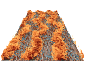
In this study, we investigate the effect of an additional Couette type shearing on the heat transfer in RB convection in an attempt to trigger the boundary layers to become fully turbulent and hence observe the transition to the ultimate regime. Figure 1 shows a flow visualization of the temperature field obtained from one of our simulations, which reveals large-scale meandering streaks that are formed near the hot plate. We performed simulations over a wide parameter range, spanning  $10^{6}\leqslant Ra\leqslant 10^{8}$ and $0\leqslant Re_{w}\leqslant 10^{4}$, while $Pr=1$ has been used in all cases, see figure 2(a). Despite the very strong forcing for the largest $Ra$ and $Re_{w}$, we did not achieve ultimate turbulence. We were limited by our requirement of using large domain sizes, as recommended by Pirozzoli et al. (Reference Pirozzoli, Bernardini, Verzicco and Orlandi2017), to ensure convergence of the main flow properties.

Figure 1. Volume rendering of the thermal structures rising from the heated plate in a simulation with  $Ra=4.6\times 10^{6}$ and $Re_{w}=8000$. The plate dimensions are $9\unicode[STIX]{x03C0}H\times 4\unicode[STIX]{x03C0}H$, in the streamwise and spanwise directions, respectively, where $H$ is the distance between the plates. The red colours show hot thermal structures emerging from the hot plate, while the blue structures show vorticity formations in the flow. For further details of the flow visualization, please see Favre & Blass (Reference Favre and Blass2019).

Figure 2. (a) Streamwise ( $n_{x}$) resolution used in the simulations as function of $Ra$ and $Re_{w}$, see table 2 for details. (b) $Re_{\unicode[STIX]{x1D70F}}$ versus $Re_{w}$ obtained from the simulations. In agreement with Pirozzoli et al. (Reference Pirozzoli, Bernardini and Orlandi2014) and Avsarkisov, Hoyas & García-Galache (Reference Avsarkisov, Hoyas and García-Galache2014) we find that $Re_{\unicode[STIX]{x1D70F}}\sim Re_{w}^{0.87}$ for large $Re_{w}$.
The remainder of this manuscript is organized as follows. In § 2 we present the simulation method. We discuss the heat transfer and skin friction measurements in §§ 3.1 and 3.2, respectively. A discussion of the identified flow regimes is given in § 4. The concluding remarks follow in § 5.
2 Simulation details
We numerically solve the three-dimensional incompressible Navier–Stokes equations within the Boussinesq approximation, which in non-dimensional form read
 $$\begin{eqnarray}\displaystyle & \displaystyle \frac{\unicode[STIX]{x2202}\boldsymbol{u}}{\unicode[STIX]{x2202}t}+\boldsymbol{u}\boldsymbol{\cdot }\unicode[STIX]{x1D735}\boldsymbol{u}=-\unicode[STIX]{x1D735}P+\left(\frac{Pr}{Ra}\right)^{1/2}\unicode[STIX]{x1D6FB}^{2}\boldsymbol{u}+\unicode[STIX]{x1D703}\hat{z},\quad \unicode[STIX]{x1D735}\boldsymbol{\cdot }\boldsymbol{u}=0, & \displaystyle\end{eqnarray}$$
 $$\begin{eqnarray}\displaystyle & \displaystyle \frac{\unicode[STIX]{x2202}\unicode[STIX]{x1D703}}{\unicode[STIX]{x2202}t}+\boldsymbol{u}\boldsymbol{\cdot }\unicode[STIX]{x1D735}\unicode[STIX]{x1D703}=\frac{1}{(PrRa)^{1/2}}\unicode[STIX]{x1D6FB}^{2}\unicode[STIX]{x1D703}, & \displaystyle\end{eqnarray}$$
 with  $\boldsymbol{u}$ the velocity non-dimensionalized by the free-fall velocity $\sqrt{g\unicode[STIX]{x1D6FD}H\unicode[STIX]{x1D6E5}}$, $t$ the time non-dimensionalized by $\sqrt{H/(g\unicode[STIX]{x1D6FD}\unicode[STIX]{x1D6E5})}$, $\unicode[STIX]{x1D703}$ the temperature non-dimensionalized by the temperature difference between the plates $\unicode[STIX]{x1D6E5}$ and $P$ the pressure non-dimensionalized by $g\unicode[STIX]{x1D6FD}\unicode[STIX]{x1D6E5}/H$. All our length scales are non-dimensionalized by $H$, implying that we set the plate distance to unity in this work.
To solve (2.1) and (2.2) we employ the second-order finite difference code AFiD (van der Poel et al. Reference van der Poel, Ostilla-Mónico, Donners and Verzicco2015), which has been validated many times against other numerical and experimental results (Verzicco & Orlandi Reference Verzicco and Orlandi1996; Verzicco & Camussi Reference Verzicco and Camussi1997, Reference Verzicco and Camussi2003; Stevens et al. Reference Stevens, Verzicco and Lohse2010, Reference Stevens, Lohse and Verzicco2011; Ostilla-Mónico et al. Reference Ostilla-Mónico, van der Poel, Verzicco, Grossmann and Lohse2014; Kooij et al. Reference Kooij, Botchev, Frederix, Geurts, Horn, Lohse, van der Poel, Shishkina, Stevens and Verzicco2018). The code uses periodic boundary conditions with uniform mesh spacing in the horizontal directions and supports a non-uniform grid distribution in the wall-normal direction. For this study, we used the GPU version of the code (Zhu et al. Reference Zhu, Phillips, Arza, Donners, Ruetsch, Romero, Ostilla-Mónico, Yang, Lohse and Verzicco2018b) to allow efficient execution of many large-scale simulations. The Couette flow forcing is realized by moving both walls in opposite directions with a velocity of  $u_{w}$, and the results for the classic Couette flow case match excellently with the results by Pirozzoli et al. (Reference Pirozzoli, Bernardini and Orlandi2014). For example, figure 2(b) shows that, for Couette flow, $Re_{\unicode[STIX]{x1D70F}}\sim Re_{w}^{0.87}$, which agrees very well with the Couette data of Pirozzoli et al. (Reference Pirozzoli, Bernardini and Orlandi2014) and Avsarkisov et al. (Reference Avsarkisov, Hoyas and García-Galache2014).
All simulations in this study were performed in a large  $9\unicode[STIX]{x03C0}H\times 4\unicode[STIX]{x03C0}H\times H$ box, in the streamwise, spanwise and wall-normal directions (Tsukahara et al. Reference Tsukahara, Kawamura and Shingai2006; Pirozzoli et al. Reference Pirozzoli, Bernardini and Orlandi2014), which is required to capture the large-scale structures formed in Couette flow (Avsarkisov et al. Reference Avsarkisov, Hoyas and García-Galache2014; Pirozzoli et al. Reference Pirozzoli, Bernardini and Orlandi2014; Lee & Moser Reference Lee and Moser2018). We adopted the grid distribution used by Pirozzoli et al. (Reference Pirozzoli, Bernardini and Orlandi2014, Reference Pirozzoli, Bernardini, Verzicco and Orlandi2017), which is based on the resolution requirements for pure buoyant flow (Shishkina et al. Reference Shishkina, Stevens, Grossmann and Lohse2010) and pure channel flow (Bernardini, Pirozzoli & Orlandi Reference Bernardini, Pirozzoli and Orlandi2014), which is very similar to our flow configuration. The average horizontal grid spacing in the mixed convection simulations is $\unicode[STIX]{x1D6E5}_{x,y}^{+}\lessapprox 4$. In the wall-normal direction the boundary layers are, on average, resolved up to $1.6$ Kolmogorov lengths. For the case at $Ra=10^{8}$ and $Re_{w}=10\,000$, i.e. the most challenging simulation of this study, we used a horizontal grid spacing of less than three wall units in both horizontal directions. There are $54$ grid points in each boundary layer to ensure that the boundary layers are resolved up to $1.3$ Kolmogorov lengths. We present a grid refinement check, which was performed in a smaller $2\unicode[STIX]{x03C0}H\times \unicode[STIX]{x03C0}H\times H$ domain to keep the test manageable, for this case in table 1. Figure 3 confirms that the simulations are fully resolved for the chosen resolution. As further validation, we show in § 3.2 that our data excellently agree with the Couette data from Pirozzoli et al. (Reference Pirozzoli, Bernardini and Orlandi2014). We make sure that all simulations have reached the statistically stationary state before collecting data. Table 2 shows the simulation parameters for the main cases presented in this study.
Table 1. Grid convergence study for  $Ra=1.0\times 10^{8}$, $Pr=1$ and $Re_{w}=10\,000$ in a $2\unicode[STIX]{x03C0}H\times \unicode[STIX]{x03C0}H\times H$ domain. $N_{x}$, $N_{y}$, $N_{z}$ indicate the resolution in the streamwise $(x)$, spanwise $(y)$ and wall-normal $(z)$ directions, respectively. The other columns show the friction Reynolds number $Re_{\unicode[STIX]{x1D70F}}$, the Monin–Obukhov length $L_{MO}/H$, the Nusselt number $Nu$ and the friction coefficient $C_{f}$. Additional information on the grid convergence study is provided in figure 3.

Table 2. Main simulations considered in this work.

3 Global flow characteristics
3.1 Effective scaling of the Nusselt number
Figure 4 shows that the heat transfer increases with increasing  $Ra$ and $Re_{w}$ and that for a given $Ra$ number a minimum heat transfer is obtained at some intermediate $Re_{w}$. Scagliarini et al. (Reference Scagliarini, Gylfason and Toschi2014) showed that the minimum is caused by the thermal plumes being swept away by the shear. Figure 5(a) shows cross-sections for constant $Ra$ which reveal that the location of the minimum heat transfer at constant $Ra$ shifts towards higher $Re_{w}$ with increasing $Ra$. For high enough $Re_{w}$, the behaviour of $Nu$ converges towards $Nu\sim 0.0013Re_{w}$. Figure 5(b), where $Nu$ is normalized by the RB value for the respective $Ra$, shows that the drop in $Nu$ becomes less pronounced and is observed at higher $Re_{w}$ when $Ra$ is increased. This is a good indication that the thermal plumes become stronger and therefore harder to disturb by the applied shear. For $Ra=10^{8}$ the decrease in $Nu$ at $Re_{w}=2000$ is only ${\sim}5\,\%$ while the data for other $Ra$ show percentages up to the high twenties. A more detailed analysis would need more data points for low $Re_{w}$, which are difficult to obtain due to the computational time that is required for each simulation.

Figure 3. Values of (a)  $Nu$ and (b) the streamwise velocity fluctuations for simulations at $Ra=10^{8}$ and $Re_{w}=10\,000$ performed using different grid resolutions. The simulations are performed in a box of $2\unicode[STIX]{x03C0}H\times \unicode[STIX]{x03C0}H\times H$ in the streamwise, spanwise and vertical directions, respectively. The displayed resolutions indicate the extrapolated streamwise resolutions that correspond to the full $9\unicode[STIX]{x03C0}H\times 4\unicode[STIX]{x03C0}H\times H$ box, see table 1 for details. Note that the simulation results are converged for the grid resolution used in this study.

Figure 4. Value of  $Nu$ as a function of $Ra$ and $Re_{w}$ in Couette–RB flow.

Figure 5. Values of (a)  $Nu$ and (b) $Nu$ normalized by the RB value $Nu_{Re_{w}=0}$ as a function of $Re_{w}$.
The results indicate that the heat transfer is influenced by the ratio of the buoyancy and shear forces. Therefore, the bulk Richardson number  $Ri$ or the above-defined Monin–Obukhov length, which take the ratio of these forces into account, are natural control and response parameters to identify the different flow regimes. Although the Monin–Obukhov theory itself is only valid for shear dominated flow, which does not necessarily exist in all our simulations, we use the Monin–Obukhov length as an objective criterion to distinguish between buoyancy and shear-driven flow. This choice builds on a long and rich tradition of using the Monin–Obukhov length to characterize mixed convective flows, namely in the seminal works by Obukhov (Reference Obukhov1946) and Monin & Obukhov (Reference Monin and Obukhov1954). Its use has significantly advanced the understanding of mixed convective flows. The Monin–Obukhov length is relevant as it characterizes the effects of both friction and buoyancy, the main physical effects in this system, by a single length scale. Also, in this case, we show that the Monin–Obukhov length is a relevant parameter that gives insight into the behaviour of the flow. From the data in table 2, we find $L_{MO}/H\approx 0.16/Ri^{\,0.91}$ (see appendix C). In figure 6(a) the Monin–Obukhov length is compared to the thermal boundary layer thickness $\unicode[STIX]{x1D706}_{\unicode[STIX]{x1D703}}$, which is determined from $\unicode[STIX]{x1D706}_{\unicode[STIX]{x1D703}}=H/(2Nu)$. Since $L_{MO}/H$ is the fraction of the domain in which the shear forcing is dominant $L_{MO}\geqslant 0.5H$ indicates when the flow is completely shear dominated. This allows us to define three different flow regimes, namely a buoyancy dominated regime ( $L_{MO}\lesssim \unicode[STIX]{x1D706}_{\unicode[STIX]{x1D703}}$), a transitional regime ( $0.5H\gtrsim L_{MO}\gtrsim \unicode[STIX]{x1D706}_{\unicode[STIX]{x1D703}}$) and a shear dominated regime ( $L_{MO}\gtrsim 0.5H$). At the moment we cannot more accurately determine the Monin–Obukhov length at which the transition takes place, but the presented ranges provide a good indication of the required thermal and shear forcing to achieve the different regimes. A similar behaviour has also been observed in convective boundary layers, where Salesky, Chamecki & Bou-Zeid (Reference Salesky, Chamecki and Bou-Zeid2017) find a cell dominated regime for $-z_{i}/L_{MO}\gtrsim 20$, where $z_{i}$ is the convective boundary layer thickness, a cell and roll dominated regime as transitional state, and a roll dominated regime for $-z_{i}/L_{MO}\lesssim 5$.

Figure 6. (a) The Monin–Obukhov length as a function of  $Ra$ for different $Re_{w}$. The Monin–Obukhov length (solid lines) is compared to the thermal boundary layer thickness (dashed lines) and to $0.5$ to define the flow regime (buoyancy dominated, transitional, shear dominated) of each simulation, see details in the text. Open symbols indicate $L_{MO}<0.5H$. (b) $Nu$ as a function of $Ra$. The numbers indicate the scaling exponent $\unicode[STIX]{x1D6FC}$ in $Nu\sim Ra^{\unicode[STIX]{x1D6FC}}$. The $\unicode[STIX]{x1D6FC}=0.37$ effective scaling line is plotted for visual reference only.
Figure 6(b) shows that the heat transfer in the buoyancy dominated regime scales as  $Nu\simeq Ra^{0.30}$, which is in agreement with results for classical RB convection ( $Re_{w}=0$, Ahlers et al. (Reference Ahlers, Grossmann and Lohse2009)). For the shear dominated regime we find that the effective scaling exponent $\unicode[STIX]{x1D6FC}$ in $Nu\sim Ra^{\unicode[STIX]{x1D6FC}}$ is $\unicode[STIX]{x1D6FC}\ll 1/3$ and in the transitional regime we find $\unicode[STIX]{x1D6FC}>1/3$. An effective scaling exponent larger than $1/3$ is one of the characteristics of the ultimate regime. It should occur when the boundary layers have transitioned to the turbulent state, which is indicated by their logarithmic profiles. Our analysis in § 4 shows that this is not yet the case in this transitional regime. Instead, for intermediate shear, the heat transfer is decreased with respect to the RB case. The locally larger effective scaling exponent simply is a consequence of the fact that with increasing $Ra$ the heat transfer, which was decreased at intermediate shear, must again converge to the RB case.
3.2 Skin friction
In figure 7 we compare the measured skin friction coefficient for different  $Re_{w}$ and $Ra$ with Prandtl’s turbulent friction law (Schlichting & Gersten Reference Schlichting and Gersten2000)
 $$\begin{eqnarray}\sqrt{\frac{2}{C_{f}}}=\frac{1}{{\mathcal{K}}}\log \left(Re_{w}\sqrt{\frac{C_{f}}{2}}\right)+C.\end{eqnarray}$$
Figure 7. (a) Skin friction coefficient  $C_{f}$ as a function of $Re_{w}$. (b) Zoom in of the grey area shown in panel (a), now on a logarithmic scale, showing the data for pure Couette flow ( $Ra=0$, stars) and $Ra=10^{6}$. Note that $C_{f}(Ra=0)$ follows the expected laminar result (- - -) until $Re_{w}=650{-}700$ and then jumps to the turbulent curve ( $\cdot \cdot \cdot$). For Couette–RB, i.e. the up-pointing triangle, no jump is observed.

Figure 8. Instantaneous snapshots of temperature fields at mid-height for a subdomain of the parameter space, see figure 2(a) and table 2, focusing on  $Ra=1.0\times 10^{6}{-}2.2\times 10^{7}$ and $Re_{w}=0{-}4000$. The panels have coloured borders depending on the flow regime they display: buoyancy dominated (white), transitional (blue) and shear dominated (orange) regime. For a more detailed quantification of the different flow fields in the presented snapshots, we refer to the values for the Monin–Obukhov length in table 2. An overview of temperature fields over the whole domain can be found in appendix A. The colour range for the snapshots in this figure and in figures 9–11 and 14 is adjusted such that the most important thermal structures are clearly visible.

Figure 9. (a)  $Ri$ versus $Re_{w}$ for different $Ra$. Open symbols indicate the presence of thin straight elongated streaks (see third snapshot from top). The dashed line indicates $L_{MO}=0.5H$. In (b) instantaneous snapshots of temperature fields at mid-height. (c) $Nu$ as a function of $Ri$ for different $Re_{w}$. An indication of the effective scaling exponent $\unicode[STIX]{x1D6FE}$ in $Nu\sim Ri^{\unicode[STIX]{x1D6FE}}$ in the different regimes is also given. For a more detailed quantification of the different flow regimes in the presented snapshots, we refer to the Monin–Obukhov lengths documented in table 2.
Following Pirozzoli et al. (Reference Pirozzoli, Bernardini and Orlandi2014) we use a von Kármán constant  ${\mathcal{K}}=0.41$ and $C=5$. The figure shows that the skin friction increases with $Ra$ and decreases with $Re_{w}$. At fixed $Ra$ the relative strength of the thermal forcing decreases for high $Re_{w}$, and therefore the obtained friction coefficient converges to the Prandtl law. This agrees very well with the findings of Scagliarini et al. (Reference Scagliarini, Einarsson, Gylfason and Toschi2015) and Pirozzoli et al. (Reference Pirozzoli, Bernardini, Verzicco and Orlandi2017) for Poiseuille–RB flow. In figure 7(b) we focus on the data for small $Re_{w}$. The skin friction in pure Couette flow follows the expected laminar result $C_{f}=4/Re_{w}$ (Pope Reference Pope2000) until a transition to the turbulent state occurs around $Re_{w}=650{-}700$. Cerbus et al. (Reference Cerbus, Liu, Gioia and Chakraborty2018) discuss that in pipe flow this jump is caused by the formation of puffs and slugs. Brethouwer, Duguet & Schlatter (Reference Brethouwer, Duguet and Schlatter2012) attribute this discontinuous jump in $C_{f}$ to the lack of restoring forces in plane Couette flow (similar to pipe, channel, and boundary layer flows). For the Couette–RB case we do not observe such a discontinuous jump. Instead, this sheared RB case is another example, next to the application of Coriolis, buoyancy and Lorentz forces discussed by Brethouwer et al. (Reference Brethouwer, Duguet and Schlatter2012), which shows that restoring forces can prevent a discontinuous jump in $C_{f}(Re_{w})$. Chantry et al. (Reference Chantry, Tuckerman and Barkley2017), on the other hand, claim that all transitions to turbulence should be continuous if the used box size is large enough. From this figure we can also judge whether the boundary layer is turbulent or not. When the slope of $C_{f}$ approaches the one of pure Couette flow the boundary layers are turbulent. We consider the boundary layer as non-turbulent when this slope starts to strongly deviate from the Prandtl law.

Figure 10. Instantaneous near-wall snapshots at  $z^{+}\approx 0.5$ of the temperature (a) and streamwise velocity (b) for $Ra=4.6\times 10^{6}$. $Re_{w}$ increases from top to bottom. For a more detailed quantification of the different flow fields in the presented snapshots, we refer to the values for the Monin–Obukhov length in table 2. The colour range for the snapshots in this figure is adjusted such that the most important thermal structures are clearly visible.
4 Local flow characteristics
4.1 Organization of turbulent structures
To further investigate the dynamics of the different regimes we show visualizations of the temperature field for all simulations in figure 8 and appendix A. We decided to show the flow at mid-height because there the flow is least affected by the walls. In the buoyancy dominated regime the primary flow structure resembles the large-scale flow found in RB convection (Stevens et al. Reference Stevens, Blass, Zhu, Verzicco and Lohse2018). In the transitional regime ( $L_{MO}\lesssim 0.5H$), the thermal forcing dominates part of the bulk where large elongated thermal plumes transform into thin straight elongated streaks when $L_{MO}$ approaches $0.5H$. In figure 8 and in appendix A this manifests itself as a very visual line diagonally through the diagram, splitting the more thermal and the more shear dominated cases. In the shear dominated regime ( $L_{MO}\gtrsim 0.5H$) we find large-scale meandering structures, similar to the ones found in pressure-driven channel flow with unstable stratification (Pirozzoli et al. Reference Pirozzoli, Bernardini, Verzicco and Orlandi2017). This significant change in flow structure can be linked to the minimum in $Nu$ in figure 5. The reason for the minimum is that at intermediate shear the thermal convection rolls are broken up, while the shear is not yet strong enough to increase the heat transfer directly. This observation is in agreement with earlier works described above (Domaradzki & Metcalfe Reference Domaradzki and Metcalfe1988; Scagliarini et al. Reference Scagliarini, Gylfason and Toschi2014, Reference Scagliarini, Einarsson, Gylfason and Toschi2015; Pirozzoli et al. Reference Pirozzoli, Bernardini, Verzicco and Orlandi2017).
In figure 9 we present a clear overview of the behaviour of the flow structures versus the flow control parameters combined in the bulk Richardson number. In panel (a), we compare the different values of  $Ri$ with the visually observed flow structures. We find a range of $Ri$ in which the flow undergoes a change from the transitional to the shear dominated regime. This happens in a range of $0.2\lesssim Ri\lesssim 0.7$. In panel (c), we can also detect this trend, where the effective scaling exponent $\unicode[STIX]{x1D6FE}$ in $Nu\sim Ri^{\unicode[STIX]{x1D6FE}}$ changes from $\unicode[STIX]{x1D6FE}=0.05\pm 0.01$ to $\unicode[STIX]{x1D6FE}=0.37\pm 0.02$. We note that more data points would be necessary to define the transition point more accurately.
Figure 9 combines these findings with the above observation that in the shear dominated regime the effective scaling exponent  $\unicode[STIX]{x1D6FC}$ in $Nu\sim Ra^{\unicode[STIX]{x1D6FC}}$ is much smaller than $1/3$, in the transitional regime $\unicode[STIX]{x1D6FC}>1/3$, and in the buoyancy dominated regime $\unicode[STIX]{x1D6FC}\simeq 0.30$. When we compare the regime transitions with the results in figure 5 it becomes clear that the lowest heat transfer for a given $Ra$ occurs at the end of the transitional regime before the emergence of the thin straight elongated streaks. Due to the large computational time that is required for each simulation the number of considered cases is limited, which makes it difficult to pinpoint exactly when the heat transfer is minimal and what the flow structure looks like in that case. However, we note that the onset of the shear dominant regime corresponds to the point where the heat transfer starts to increase as the additional shear can then more effectively enhance the overall heat transport.
To get more insight into the boundary layer dynamics in the different regimes, we show the temperature and streamwise velocity at the boundary layer height for $Ra=4.6\times 10^{6}$ in figure 10. At this Rayleigh number the flow is in the transitional regime for $Re_{w}=2000$ and $Re_{w}=3000$, and in the shear dominant regime for $Re_{w}\geqslant 4000$. For all cases we observe a clear imprint of the large-scale structures observed at mid-height, see figure 8 and appendix A. This indicates that the large-scale dynamics has a pronounced influence on the flow structures in the boundary layers (Stevens et al. Reference Stevens, Blass, Zhu, Verzicco and Lohse2018). The figure also reveals that in the transitional and shear dominated regimes the lowest temperatures at boundary layer height are observed in the high-speed streak regions, which indicates that the regions with the highest shear contribute most to the overall heat flux.
4.2 Flow statistics
We now present the streamwise temperature variance spectra  $E_{\unicode[STIX]{x1D703}}(k)$ in figure 11 to analyse the size of the large-scale structures as function of the Monin–Obukhov length. The position of the peak in the temperature spectrum indicates the wavelength of the most prominent thermal structure (Stevens et al. Reference Stevens, Blass, Zhu, Verzicco and Lohse2018). In panels (b,c) we plot the evolution of these wavelengths versus the absolute size of the flow domain. Therefore we define $k_{x_{peak}}$ and $k_{y_{peak}}$ as the wavenumbers of the peak in the respective energy spectrum and $\ell _{x}=2\unicode[STIX]{x03C0}/k_{x_{peak}}$ and $\ell _{y}=2\unicode[STIX]{x03C0}/k_{y_{peak}}$ as the respective wavelengths. If the spectrum does not show a clear peak but keeps growing for small $k$, the structure size is limited by the box size, which is $\unicode[STIX]{x1D6E4}_{x}=9\unicode[STIX]{x03C0}$ in streamwise (figure 11b) and $\unicode[STIX]{x1D6E4}_{y}=4\unicode[STIX]{x03C0}$ in spanwise direction (figure 11c).

Figure 11. (a) Overview of streamwise temperature variance spectra at mid-height at  $Ra=4.6\times 10^{6}$ for the different flow regimes. Panels (b,c) show the evolution of peaks in streamwise and spanwise temperature variance spectra, respectively, versus the Monin–Obukhov length. The spectra were evaluated on three-dimensional snapshots and are subsequently time averaged.
For  $L_{MO}\rightarrow \infty$, $\ell _{x}\approx \unicode[STIX]{x1D6E4}_{x}H$, which is expected since for pure Couette flow, structures much larger than $9\unicode[STIX]{x03C0}$ are expected (Lee & Moser Reference Lee and Moser2018). $\ell _{y}\approx 0.8\unicode[STIX]{x03C0}H=0.2\unicode[STIX]{x1D6E4}_{y}H$ for the highest shear case, but here more data points are needed for a clearer determination of its behaviour. In the other limit of $L_{MO}\rightarrow 0$, i.e. in the transitional regime as the RB case (buoyancy dominated regime) is not shown due to the logarithmic axis, the large-scale structures are elongated over the whole streamwise length, which is consistent with figures 8 and 14. For pure RB convection, where $L_{MO}=0$, $\ell _{x}$ decreases to $\ell _{x}\approx 2\unicode[STIX]{x03C0}H$, which is in agreement with Stevens et al. (Reference Stevens, Blass, Zhu, Verzicco and Lohse2018). In the spanwise direction, the flow converges already much earlier to the RB case where $\ell _{y}\approx 2\unicode[STIX]{x03C0}H=0.5\unicode[STIX]{x1D6E4}_{y}H$. In the shear dominated regime, where the flow meanders, the structure size in streamwise direction drops to about half the box length. In the spanwise direction, this flow regime is present as a local peak in panel (c). Due to the minimal number of data points, it is not possible to fully assess the behaviour of $\ell _{x}$ and $\ell _{y}$ versus $L_{MO}$ for all $Ra$ and $Re_{w}$. Nevertheless, the minimum in $\ell _{x}$ and peak in $\ell _{y}$ in the shear dominated regime are very distinct.
To further quantify the cases shown in figure 10, in figure 12 we show the streamwise velocity and temperature profiles for fixed  $Ra=4.6\times 10^{6}$ and increasing $Re_{w}$ from $2000$ to $10\,000$. As can be seen, for the wall Reynolds number in the transitional range up to $Re_{w}\approx 4000$ (see corresponding curve in figure 9a) neither the temperature nor the streamwise velocity profiles are logarithmic. This indicates that the boundary layers are not yet turbulent in this state. Hence, the higher $Nu$ scaling in this transitional regime is not caused by a triggered transition to the ultimate regime. Note that spatio-temporally chaotic flow with thermal plume detachment from the walls must not be confused with turbulent flow. The temporal fluctuations in this regime can in fact be considerable, but given the small shear Reynolds numbers, the flow is still not turbulent. Here we use the definition of turbulence as absence of large-scale coherence in space and time.

Figure 12. (a) Mean streamwise velocity and (b) temperature profiles, where  $u^{+}=u/u_{\unicode[STIX]{x1D70F}}$ and, following Pirozzoli et al. (Reference Pirozzoli, Bernardini, Verzicco and Orlandi2017), $T^{+}=T/T_{\unicode[STIX]{x1D70F}}$ with the friction temperature $T_{\unicode[STIX]{x1D70F}}=Q/u_{\unicode[STIX]{x1D70F}}$ for $Ra=4.6\times 10^{6}$.
In contrast, in the shear dominated regime (beyond  $Re_{w}\approx 4000$ for this $Ra=4.6\times 10^{6}$) the streamwise velocity and temperature profiles do start to converge to a logarithmic profile with further increasing $Re_{w}$, reflecting the onset of the ultimate regime. This observation is in agreement with previous findings for Couette–RB (Liu Reference Liu2003; Choi, Chung & Kim Reference Choi, Chung and Kim2004; Debusschere & Rutland Reference Debusschere and Rutland2004; Le & Papavassiliou Reference Le and Papavassiliou2006) and Poiseuille–RB (Scagliarini et al. Reference Scagliarini, Einarsson, Gylfason and Toschi2015; Pirozzoli et al. Reference Pirozzoli, Bernardini, Verzicco and Orlandi2017).
In figure 13 we show the same statistical quantities as in figure 12, but now for fixed  $Re_{w}=6000$. For $Ra\gtrsim 10^{7}$ the flow is in the transitional regime and for $Ra\lesssim 10^{7}$ the flow undergoes a transition into the shear dominated regime. Just as in figure 12 we observe that the temperature and streamwise velocity profiles are not logarithmic in the transitional regime. As the Richardson number decreases with decreasing $Ra$, we see that the profiles converge towards a logarithmic behaviour. From a comparison with table 2 we find that $Ri\lesssim 0.2$ seems to be required to achieve logarithmic temperature and velocity profiles. A comparison with the results shown in figure 9 confirms that $Ri\approx 0.2$ is indeed the threshold where the flow undergoes its transition to the shear dominated regime. This is also consistent with the work of Pirozzoli et al. (Reference Pirozzoli, Bernardini, Verzicco and Orlandi2017), who report a regime with the increased importance of friction at $Ri\approx 0.1$. For the parameter regime under investigation, the effective scaling exponent $\unicode[STIX]{x1D6FC}$ in the shear dominated regime is well below $1/3$. In both figures we can detect a non-monotonic behaviour of both $u^{+}$ and $T^{+}$ for low $Re_{w}$ and high $Ra$. The non-monotonic temperature profile indicates the formation of different flow layers, i.e. heat that is carried by hot plumes originating from the bottom plate gets entrapped somewhere in the middle of the domain. Similarly, some of the cold plumes originating from the top plate also get trapped. Several further statistical quantities are presented in appendix B.

Figure 13. (a) Mean streamwise velocity and (b) temperature profiles, where  $u^{+}=u/u_{\unicode[STIX]{x1D70F}}$ and $T^{+}=T/T_{\unicode[STIX]{x1D70F}}$ with $T_{\unicode[STIX]{x1D70F}}=Q/u_{\unicode[STIX]{x1D70F}}$ for $Re_{w}=6000$. $T_{Ra=0}^{+}$ was determined through a passive-scalar temperature field.
5 Concluding remarks
We performed direct numerical simulations of turbulent thermal convection with Couette type flow shearing. We presented cases in a range  $10^{6}\leqslant Ra\leqslant 10^{8}$ and $0\leqslant Re_{w}\leqslant 10^{4}$, achieving up to $Re_{\unicode[STIX]{x1D70F}}\approx 710$. For fixed Rayleigh number we obtain a non-monotonic progression of $Nu$ similarly to what was previously observed in unstable stratification with a pressure gradient (Scagliarini et al. Reference Scagliarini, Gylfason and Toschi2014). The addition of imposed shear to thermal convection first leads to a reduction of the heat transport by disrupting the turbulent system before the shear becomes strong enough to create meandering streaks that efficiently transport the heat away from the wall. As the impact of the thermal plumes on the flow decreases with increasing shear, the skin friction coefficient at constant $Ra$ drops with increasing $Re_{w}$.
Using the Monin–Obukhov length  $L_{MO}$ and the thermal boundary layer thickness $\unicode[STIX]{x1D706}_{\unicode[STIX]{x1D703}}$, we identify three flow regimes. In the buoyancy dominated regime ( $L_{MO}\lesssim \unicode[STIX]{x1D706}_{\unicode[STIX]{x1D703}}$) large thermal plumes dominate the flow. With decreasing Richardson number we first find a transitional regime ( $0.5H\gtrsim L_{MO}\gtrsim \unicode[STIX]{x1D706}_{\unicode[STIX]{x1D703}}$), before the shear dominated flow regime with large-scale meandering streaks is obtained. For given $Ra$ the minimum heat transport is found before the onset of this shear dominated regime when thin straight elongated streaks dominate the flow. We find that in the transitional regime the effective scaling exponent $\unicode[STIX]{x1D6FC}$ in $Nu\sim Ra^{\unicode[STIX]{x1D6FC}}$ is larger than $1/3$. An analysis of the flow characteristics shows that the temperature and streamwise velocity profiles are not logarithmic in this transitional regime, which one would expect when this high scaling exponent would indicate the onset of the ultimate regime. We want to investigate in future studies whether it is possible to further increase the thermal and sheared forcing far enough to trigger the occurrence of a logarithmic velocity profile in the boundary layer and thus the ultimate convection in Couette–RB, but considerably more CPU time is required for that.

Figure 14. Instantaneous snapshots of all simulated temperature fields at mid-height, see the caption of figure 8 for further details.
Acknowledgements
We thank C.-C. Caulfield, D. Chung and S. Yerragolam for fruitful discussions and J. M. Favre for his support with three-dimensional data visualizations, which resulted in figure 1. The simulations were supported by a grant from the Swiss National Supercomputing Centre (CSCS) under project ID s713, s802 and s874. This work was financially supported by NWO, by the Dutch center for Multiscale Catalytic Energy Conversion (MCEC) and the Priority Programme SPP 1881 ‘Turbulent Superstructures’ of the Deutsche Forschungsgemeinschaft. D.L. gratefully acknowledges support from ERC (the European Research Council) through an ERC Advanced Grant ‘Diffusive Droplet Dynamics’ (project number 740479). R.J.A.M. gratefully acknowledges support through an ERC Starting Grant ‘UltimateRB’ (project number 804283). Part of the work was carried out on the national e-infrastructure of SURFsara, a subsidiary of SURF cooperation, the collaborative ICT organization for Dutch education and research.
Declaration of interests
The authors report no conflict of interest.
Appendix A. Flow field overview
As an addition to figure 8 we present in figure 14 the full overview of temperature snapshots at mid-height, ranging from  $Ra=1.0\times 10^{6}{-}1.0\times 10^{8}$ and $Re_{w}=0{-}10\,000$. All three regimes, i.e. the buoyancy dominated regime, the transitional regime and the shear dominated regime, can be observed here.
Appendix B. Further flow statistics
In addition to the data presented in figures 12 and 13 we present further flow statistics here. Figure 15 shows the velocity and temperature fluctuations as function of height for  $Ra=4.6\times 10^{6}$ for various wall shear Reynolds numbers. It can be observed that the velocity fluctuations increase with $Re_{w}$. The temperature fluctuations show a non-monotonic behaviour. The peak temperature fluctuations first increase with increasing $Re_{w}$ before the peak of the temperature fluctuations decreases with increasing wall shear. Figure 16 shows the velocity and temperature fluctuations for $Re_{w}=6000$ and increasing $Ra$.
$Ra$.  $u_{peak}$ and $v_{peak}$ first increase and then monotonically decrease with increasing $Ra$ when thermal forcing is added to Couette flow. Both the wall-normal velocity and the temperature fluctuations decrease completely monotonically for increasing thermal forcing.

Figure 15. Fluctuations of (a) streamwise, (b) spanwise and (c) wall-normal velocities, and (d) temperature for  $Ra=4.6\times 10^{6}$.

Figure 16. Fluctuations of (a) streamwise, (b) spanwise and (c) wall-normal velocities, and (d) temperature for  $Re_{w}=6000$. $\overline{T^{\prime 2}}_{Ra=0}$ was determined through a passive-scalar temperature field.

Figure 17. Value of  $L_{MO}/H$ versus $Ri$ and the corresponding fit $L_{MO}/H=0.16/Ri^{\,0.91}$ to the data.

Figure 18. Value of  $L_{MO}$ normalized by the thermal boundary layer thickness $\unicode[STIX]{x1D706}_{\unicode[STIX]{x1D703}}$ versus $Re_{w}$. For $L_{MO}/\unicode[STIX]{x1D706}_{\unicode[STIX]{x1D703}}\lesssim 1$ the flow is in the buoyancy dominated regime.
Appendix C. Scaling of the Monin–Obukhov length with Richardson number
In figure 17 we present the Monin–Obukhov length  $L_{MO}$ versus the Richardson number $Ri$ for all simulations. We find that the Monin–Obukhov length scales as $L_{MO}/H=0.16/Ri^{\,0.91}$, similar to $L_{MO}/H=0.15/Ri^{\,0.85}$ as found by Pirozzoli et al. (Reference Pirozzoli, Bernardini, Verzicco and Orlandi2017) for channel flow with unstable stratification.
Appendix D. Comparison of  $L_{MO}$ and $\unicode[STIX]{x1D706}_{\unicode[STIX]{x1D703}}$


In figure 18 we show the ratio between the Monin–Obukhov length  $L_{MO}$ and the thermal boundary layer thickness $\unicode[STIX]{x1D706}_{\unicode[STIX]{x1D703}}$, which is determined from $\unicode[STIX]{x1D706}_{\unicode[STIX]{x1D703}}=H/(2Nu)$. For $L_{MO}/\unicode[STIX]{x1D706}_{\unicode[STIX]{x1D703}}<1$ the flow is in the buoyancy dominated regime. For higher $L_{MO}/\unicode[STIX]{x1D706}_{\unicode[STIX]{x1D703}}$, the flow first reaches the transitional regime before the shear dominated regime is reached, where $L_{MO}/\unicode[STIX]{x1D706}_{\unicode[STIX]{x1D703}}\sim Re_{w}^{5/2}$.


 Open access