


1. Introduction
The resolvent, the transfer function of a linear system with constant coefficients, describes the response of such a system to sustained perturbations or forcing inputs. The analysis of a resolvent provides insights of the dominant directions in which the perturbation can be amplified (Trefethen & Embree Reference Trefethen and Embree2005). Trefethen et al. (Reference Trefethen, Trefethen, Reddy and Driscoll1993) applied resolvent analysis to laminar Poiseuille flows to study the subcritical laminar–turbulent transition caused by the significant transient growth in perturbation energy. McKeon & Sharma (Reference McKeon and Sharma2010) extended the resolvent analysis for turbulent pipe flow, where the flow is linearized about the statistically stationary turbulent mean flow and regarded the retaining nonlinear terms as an internal forcing. By analysing the resolvent of the linearized system, they proposed a reduced-order model to capture the coherent structures in wall-bounded turbulence. Later in several studies (Moarref et al. Reference Moarref, Sharma, Tropp and McKeon2013; Sharma & McKeon Reference Sharma and McKeon2013; Karban et al. Reference Karban, Martini, Cavalieri, Lesshafft and Jordan2022) similar approaches have been taken following this resolvent formulation for analysing the coherent structures in the wall turbulence in a channel. The resolvent analysis of turbulent jets has also been investigated (Jeun, Nichols & Jovanović Reference Jeun, Nichols and Jovanović2016; Schmidt et al. Reference Schmidt, Towne, Rigas, Colonius and Brès2018; Pickering et al. Reference Pickering, Rigas, Schmidt, Sipp and Colonius2021) for studying the corresponding coherent structures and jet noise. Skene et al. (Reference Skene, Yeh, Schmid and Taira2022) developed a sparsity-promoting resolvent formulation to determine the actuation locations for external turbulent flow control by revealing spatially localized structures sensitive to energy amplification.
Due to the capability of providing dominant and subdominant modes of flow to construct a reduced-order model, resolvent analysis is often used to design an effective flow control technique for the flow over a stationary body or boundary such as flows over a cavity (Rowley et al. Reference Rowley, Williams, Colonius, Murray and Macmynowski2006; Gómez et al. Reference Gómez, Blackburn, Rudman, Sharma and McKeon2016; Gómez & Blackburn Reference Gómez and Blackburn2017; Liu et al. Reference Liu, Sun, Yeh, Ukeiley, Cattafesta III and Taira2021) or flows over a stationary body (Yeh & Taira Reference Yeh and Taira2019; Jin, Illingworth & Sandberg Reference Jin, Illingworth and Sandberg2020). Luhar, Sharma & Mckeon (Reference Luhar, Sharma and Mckeon2014) applied opposition control on turbulent channel flow using the resolvent analysis framework. Brunton & Noack (Reference Brunton and Noack2015) reviewed the progress of closed-loop turbulence control and selected resolvent-analysis-based control as one of the successful closed-loop flow controls. Yeh & Taira (Reference Yeh and Taira2019) applied resolvent analysis to design an active control for separated flow of NACA0012 airfoils with fixed angles of attack. The control successfully makes the separated flow reattach, which leads to a drag reduction of 38 % for the best case. Jin et al. (Reference Jin, Illingworth and Sandberg2020) investigated feedback control of vortex shedding of a cylinder at low Reynolds numbers based on a reduced-order transfer function modelled from the resolvent operator. The resulting feedback controllers are capable of stabilizing the system up to  ${\textit {Re}}=100$ but their performance deteriorates rapidly with increasing Reynolds number. Liu et al. (Reference Liu, Sun, Yeh, Ukeiley, Cattafesta III and Taira2021) implemented a resolvent-analysis-based design tool for unsteady control of supersonic turbulent flow in a fixed cavity. The designed control manages to reduce the pressure fluctuation in the cavity by 52 %. Martini et al. (Reference Martini, Jung, Cavalieri, Jordan and Towne2022) applied the resolvent-based method to the Wiener–Hopf problem and developed optimal estimation and control techniques for the application of flow over backward-facing steps. Besides application in active control, Pfister, Fabbiane & Marquet (Reference Pfister, Fabbiane and Marquet2022) applied resolvent analysis to the investigation of boundary layer instability attenuation by viscoelastic patches.
The resolvent was originally derived from the frequency response of a linear time-independent (LTI) system. In order to extend resolvent analysis to a linear time-dependent system, the time convolution between the state and the linear operator needs to be simplified when performing Fourier transform on the linear time-dependent system (Padovan, Otto & Rowley Reference Padovan, Otto and Rowley2020; Yeh, Gopalakrishnan Meena & Taira Reference Yeh, Gopalakrishnan Meena and Taira2021). Yeh et al. (Reference Yeh, Gopalakrishnan Meena and Taira2021) developed a modal analysis technique based on the Katz centrality to investigate a time-evolving network of vortical interactions on time-varying base flow. By perturbing the flow with the resulting broadcast mode, the evolution of a two-dimensional decaying isotropic turbulence is effectively modified. Padovan et al. (Reference Padovan, Otto and Rowley2020) studied the input–output characteristics of systems linearized about a time-periodic base flow via the harmonic resolvent, which utilizes truncated Fourier series with a fundamental harmonic frequency to express the response of such a linear time-periodic (LTP) system. They applied harmonic resolvent analysis to the flow over an airfoil at a near-stall angle of attack and introduced a small-amplitude sinusoidal vertical motion at the vortex shedding frequency to the airfoil as the near-body periodic forcing. Padovan & Rowley (Reference Padovan and Rowley2022) further extended harmonic resolvent analysis to study subharmonic dynamics of a forced incompressible axisymmetric jet. Since in the above two studies the vortex shedding frequency is the only dominant frequency, the harmonic resolvent is able to describe accurately the flow structures developed in response to periodic forcing. However, for a LTP system with more than one dominant frequency, it is difficult to determine not only a specific frequency for the harmonic resolvent but also the number of terms in the expansion that are needed to capture important flow dynamics. In this case, Wereley (Reference Wereley1991) provided a mathematically equivalent theory based on the Floquet theory.
In this study, we propose a general resolvent analysis framework inspired by Wereley (Reference Wereley1991) and Yeh & Taira (Reference Yeh and Taira2019) for a LTP system with complex dynamics that has more than one dominant frequency based on the Floquet theory. A demonstrative example of the flow around a sinusoidal plunging cylinder is selected to develop a design tool for flow control using this Floquet resolvent analysis. In this framework, the Lyapunov–Floquet transformation is used to transform the LTP system to a similar LTI system, which retains all important dynamics. Then the resolvent-analysis-based design tool developed by Yeh & Taira (Reference Yeh and Taira2019) for a LTI system can be implemented on the transformed LTI system to formulate an input–output process in frequency space and design an effective active flow control for the flow around a sinusoidal plunging cylinder.
2. Problem set-up
2.1. Problem description
We consider a circular cylinder plunging in an unbounded free stream at a low Reynolds number  ${\textit {Re}} = U_\infty D/\nu = 500$ as shown in figure 1, where $U_\infty$ is the free-stream velocity, $D$ is the diameter of the cylinder and $\nu$ is the kinematic viscosity. Since the Reynolds number is low, the flow around the cylinder is assumed to be quasi-two-dimensional. The analysis is therefore performed on a two-dimensional cross-section of the cylinder. The cylinder undergoes a sinusoidal plunging motion with an amplitude of $0.1D$ at a frequency of $f_p$. The Strouhal number of the plunging motion is set to be $St_p = f_pD/U_\infty = 0.36$, which is 1.5 times the natural shedding frequency at ${\textit {Re}} = 500$. Therefore, the dimensionless plunging velocity of the cylinder scaled by $U_\infty$ can be expressed as $\boldsymbol {U}(t) = 0.1 \omega _p\cos (\omega _p t) \hat {\boldsymbol {y}}$, where $\omega _p=2{\rm \pi} St_p$ is the dimensionless angular velocity, $\hat {\boldsymbol {y}}$ is the transversal unit vector and $t$ is the dimensionless time scaled by $D/U_\infty$. The above parameters are selected based on Bao et al. (Reference Bao, Chen, Liu, Li and Wang2012) so that the resulting flow does not lock in with the plunging motion and results in a high lift fluctuation, which is aimed to be reduced in this study.

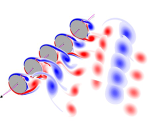
Figure 1. A cylinder plunging in a free stream with localized body forces as actuators.
2.2. Resolvent analysis domain and flow control set-up
In order to extend the resolvent analysis, which only applies to stationary bodies/boundaries, to a moving body, the analysis and simulations are done in a frame of reference fixed on the centre of the cylinder. As shown in figure 1, the resolvent analysis is performed in a limited domain of  $7D\times 3D$ around the cylinder in the cylinder-fixed frame, which is located respectively at $1D$ and $1.5D$ from the left and bottom boundary. In order to mimic the actual actuators, two body forces, each in the dimensionless form of
 \begin{equation} \boldsymbol{f}_a = A\left[ 1 - \cos\left(\omega^+ t\right)\right] g\left(\boldsymbol{x}_a, \xi \right) \hat{\boldsymbol{e}}_a , \end{equation}
are placed at  $\boldsymbol {x}_a = (r,\theta ) = (0.5+6\xi /D,\pm 105^\circ )$, where $A$ is the amplitude of the body force, $\omega ^+ = 2{\rm \pi} St^+$ is the dimensionless angular velocity of the actuation, $St^+$ is the Strouhal number of the actuation, $r$ is the dimensionless distance from the cylinder centre scaled by $D$,
$D$,  $\theta$ is the angle between the actuation location and the leading edge, $g(\boldsymbol {x}_a,\xi )$ is the Gaussian function with a width of $\xi$ located at $\boldsymbol {x}_a$ and $\hat {\boldsymbol {e}}_a$ is the unit vector in the actuating direction. The amplitude $A$ and the width of the Gaussian $\xi$ can be adjusted to generate a certain value of the momentum coefficient, which is defined as $C_\mu = u_{{jet}}^2 \xi /(\tfrac {1}{2}U_\infty ^2D)$, where $u_{{jet}}$ is the time-averaged jet speed measured in the absence of free stream.
2.3. Simulation set-up and the base flow
In order to simulate the incompressible flow and perform resolvent analysis in the cylinder-fixed frame, the following incompressible vorticity equation and boundary conditions in the cylinder-fixed frame derived by Lin, Hsieh & Tsai (Reference Lin, Hsieh and Tsai2021) are used:
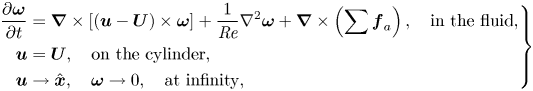 \begin{equation} \left. \begin{aligned} \displaystyle\frac{\partial\boldsymbol{\omega}}{\partial t} & = \boldsymbol{\nabla}\times\left[\left(\boldsymbol{u}-\boldsymbol{U}\right)\times\boldsymbol{\omega}\right] + \frac{1}{{\textit{Re}}}\nabla^2\boldsymbol{\omega} + \boldsymbol{\nabla}\times\left(\sum\boldsymbol{f}_a\right), \quad \text{in the fluid},\\ \displaystyle \boldsymbol{u} & = \boldsymbol{U}, \quad \text{on the cylinder},\\ \displaystyle \boldsymbol{u} & \rightarrow \hat{\boldsymbol{x}}, \quad \boldsymbol{\omega} \rightarrow 0, \quad \text{at infinity}, \end{aligned} \right\} \end{equation}
where  $\boldsymbol {u}$ and $\boldsymbol {\omega }$ scaled respectively by $U_\infty$ and $U_\infty /D$ are the dimensionless laboratory-frame flow velocity and vorticity, $\boldsymbol {U}$ is the plunging velocity described in § 2.1, $\hat {\boldsymbol {x}}$ is the unit vector in the streamwise direction and $\boldsymbol {\nabla }\times (\sum \boldsymbol {f}_a)$ collects the external forcing inputs. In general, (2.2) can be extend to flows around a body undergoing any rigid-body motion by replacing $\boldsymbol {U}$ with the combination of translational and rotational velocity of the motion. Therefore, the current analysis can be easily extended to analyse flows around a body undergoing not only periodic plunging motion, but also periodic surging, or pitching motions.
Equation (2.2) is solved using the immersed boundary projection method (IBPM) developed by Colonius & Taira (Reference Colonius and Taira2008), which uses a nullspace approach and multi-domain far-field boundary conditions, but now with the convective term being replaced by  $\boldsymbol {\nabla }\times [(\boldsymbol {u}-\boldsymbol {U})\times \boldsymbol {\omega }]$. In all simulations, the IBPM is implemented in six domains with the domain being magnified and the grid being coarsened by a factor of 2 at each grid level, and the first (smallest, finest) domain coincides with the resolvent analysis domain and is discretized on a two-dimensional Cartesian staggered grid with equal grid spacing $\Delta x = \Delta y = 0.01 D$. The resulting number of discrete disturbed vorticities in one domain is $n=699\times 299 = 209\,001$. The width of the Gaussian $\xi$ for the body force described in § 2.2 and the spacing between two adjacent immersed boundary points are set to be equal to the grid spacing. The time increment $\Delta t$ is set to keep the Courant–Friedrichs–Lewy number less than 0.4.
Figure 2(a) shows the vorticity field time-averaged from  $t=10T$ to $15T$, where $T = 1/St_p$ is the dimensionless plunging period scaled by $D/U_\infty$. This time-averaged flow serves as a time-independent base flow for linear analysis of (2.2). The time-averaged flow in figure 2(a) should be symmetric; however, in this case the convergence is slow to achieve symmetry within a practical run time. Figure 2(b) shows the lift and drag coefficients of the plunging and stationary cylinders in the corresponding time period. The fluctuation in lift coefficient is greater for a plunging cylinder than a stationary one, while the drag coefficients for plunging and stationary cylinders vary roughly in the same range. Therefore, this study focuses on designing an effective active control to reduce the lift fluctuation using resolvent analysis. Figure 2(c) depicts the spectrum of the lift coefficient of the plunging cylinder. Therefore, the flow around the plunging cylinder is quasi-periodic with three dominant frequencies at $St = 0.36$, 0.216 and 0.072, which correspond respectively to the frequencies of plunging motion, vortex shedding and the envelope of those two waves. Figure 2(d) reveals the phase plot between the lift coefficient of the plunging cylinder and the transversal displacement of the plunging motion, which shows that the flow does not lock in to the plunging motion.

Figure 2. (a) Vorticity field time-averaged from  $t=10T$ to $15T$. Positive and negative vorticity contour levels are plotted respectively in solid and dash-dotted curves. (b) The lift and drag coefficients of plunging and stationary cylinders in $t\in [10T,15T]$. (c) The spectrum of the lift coefficient. (d) The phase plot of the lift coefficient and the transversal displacement.
3. Resolvent analysis for a plunging cylinder
3.1. Derivation of the LTP system
First, we apply the Reynolds decompositions  $\boldsymbol {u} = \bar {\boldsymbol {u}} + \boldsymbol {u}'$ and $\boldsymbol {\omega } = \bar {\boldsymbol {\omega }} + \boldsymbol {\omega }'$ to (2.2), where $\bar {\boldsymbol {u}}$ and $\bar {\boldsymbol {\omega }}$ are respectively the velocity and vorticity fields of the time-independent base flow described in § 2.3 and $\boldsymbol {u}'$ and $\boldsymbol {\omega }'$ are respectively the disturbed velocity and vorticity fields. Equation (2.2) yields
 \begin{equation} \left. \begin{aligned} \displaystyle\frac{\partial\boldsymbol{\omega}'}{\partial t} & = \boldsymbol{\nabla}\times\left[ \boldsymbol{\mathcal{L}}(\boldsymbol{\omega}') + \boldsymbol{F} \right], \quad \text{in the fluid},\\ \displaystyle \boldsymbol{u}' & = \boldsymbol{U} - \bar{\boldsymbol{u}}, \quad \text{on the cylinder},\\ \displaystyle \boldsymbol{u}' & \rightarrow 0, \quad \boldsymbol{\omega}' \rightarrow 0, \quad \text{at infinity}, \end{aligned} \right\} \end{equation}
where  $\boldsymbol {\mathcal {L}}(\boldsymbol {\omega }') = (\bar {\boldsymbol {u}}-\boldsymbol {U})\times \boldsymbol {\omega }' + \boldsymbol {u}'\times \bar {\boldsymbol {\omega }} - ({1}/{{\textit {Re}}})\boldsymbol {\nabla }\times \boldsymbol {\omega }'$ collects the linear operations for $\boldsymbol {\omega }'$, $\boldsymbol {f}_{{int}} = (\bar {\boldsymbol {u}}-\boldsymbol {U})\times \bar {\boldsymbol {\omega }} + \boldsymbol {u}'\times \boldsymbol {\omega }' - ({1}/{{\textit {Re}}})\boldsymbol {\nabla }\times \bar {\boldsymbol {\omega }}$ collects the nonlinear operations for $\boldsymbol {\omega }'$ and the base-flow terms, $\boldsymbol {f}_{{ext}} = \sum \boldsymbol {f}_a$ collects the external control forcing and $\boldsymbol {F} = \boldsymbol {f}_{{int}} +\boldsymbol {f}_{{ext}}$. Since $\boldsymbol {U}$ is $T$-periodic and $\bar {\boldsymbol {u}}$ and $\bar {\boldsymbol {\omega }}$ are time-independent, the linear operator $\boldsymbol {\mathcal {L}}(\boldsymbol {\omega }')$ is $T$-periodic. Here, unlike in the traditional Floquet stability analysis, (3.1) does not come from linearizing (2.2) about a phase-averaged base flow. As discussed in § 2.3, the base flow is only quasi-periodic and its period is not $T$ either. Therefore, the linear operator $\boldsymbol {\mathcal {L}}(\boldsymbol {\omega }')$ will not be $T$-periodic if (2.2) is linearized about the base flow phase-averaged over one plunging period.
McKeon & Sharma (Reference McKeon and Sharma2010) treated equation (3.1) as a linear system of  $\boldsymbol {\omega }'$ with $\boldsymbol {\nabla }\times \boldsymbol {F}$ as a forcing input. Moreover, $\boldsymbol {f}_{{int}}$ is interpreted as the internal forcing input due to the nonlinear and viscous interaction in the flow. Again, (3.1) can be solved using the IBPM developed by Colonius & Taira (Reference Colonius and Taira2008) with the convective term being replaced by $\boldsymbol {\nabla }\times [ (\bar {\boldsymbol {u}}-\boldsymbol {U})\times \boldsymbol {\omega }' + \boldsymbol {u}'\times \bar {\boldsymbol {\omega }} ]$ and the addition of the forcing term $\boldsymbol {\nabla }\times \boldsymbol {F}$. From (3.1), Yeh & Taira (Reference Yeh and Taira2019) were able to obtain the resolvent of the linear system directly by expanding the disturbed flow quantities as the sum of Fourier modes because the operator $\boldsymbol {\mathcal {L}}(\boldsymbol {\omega }')$ in their system is time-independent. However, (3.1) is now time-periodic for the flow around a plunging cylinder so that an additional similarity transformation, the Lyapunouv–Floquet transformation, is required to transform equation (3.1) into a similar linear system with time-invariant coefficients in order to apply the resolvent analysis.
3.2. Derivation of the LTI system
We discretize equation (3.1) spatially on the Cartesian staggered grid described in § 2.3, which yields
 \begin{equation} \left. \begin{aligned} \displaystyle\frac{{\rm d}\kern0.7pt \boldsymbol{x}}{{\rm d}t} & = \boldsymbol{\mathsf{A}}(t)\boldsymbol{x} + \boldsymbol{g}, \quad \text{in the fluid},\\ \displaystyle \mathcal{C}(\mathcal{C}^T\mathcal{C})^{{-}1}\boldsymbol{x} & = {\mathcal{C}^T}^+\boldsymbol{x} = \boldsymbol{U} - \bar{\boldsymbol{u}}, \quad \text{on the cylinder},\\ \displaystyle {\mathcal{C}^T}^+\boldsymbol{x} & \rightarrow 0, \quad \boldsymbol{x} \rightarrow \boldsymbol{0}, \quad \text{at infinity}, \end{aligned} \right\} \end{equation}
where  $\boldsymbol {x}(t)$ is the discrete disturbed vorticity in the resolvent analysis domain and $\boldsymbol{\mathsf{A}}(t)\boldsymbol {x}$ and $\boldsymbol {g}$ are respectively the spatial discretization of $\boldsymbol {\nabla }\times \boldsymbol {\mathcal {L}}(\boldsymbol {\omega }')$ and $\boldsymbol {\nabla }\times \boldsymbol {F}$. The operator $\mathcal {C}$ is the discrete curl operator used in Colonius & Taira (Reference Colonius and Taira2008) and the operator ${\mathcal {C}^T}^+ = \mathcal {C}(\mathcal {C}^T\mathcal {C})^{-1}$ is the right pseudo-inverse of $\mathcal {C}^T$, which maps the discrete vorticity to the corresponding discrete velocity. The operation $\boldsymbol {q} = \mathcal {C}(\mathcal {C}^T\mathcal {C})^{-1}\boldsymbol {x}$ is equivalent to first solving the Poisson equation $\mathcal {C}^T\mathcal {C}\boldsymbol {s} = \boldsymbol {x}$ (the discretization of $\boldsymbol {\nabla }\times \boldsymbol {\nabla }\times \boldsymbol {\psi } = \boldsymbol {\omega }'$) for the discrete streamfunction $\boldsymbol {s}$, and then taking the curl of the discrete streamfunction to obtain the discrete velocity, i.e. $\boldsymbol {q} = \mathcal {C}\boldsymbol {s}$ (the discretization of $\boldsymbol {\nabla }\times \boldsymbol {\psi } = \boldsymbol {u}$). Since the linear operator $\boldsymbol {\mathcal {L}}(\boldsymbol {\omega }')$ is $T$-periodic, the linear coefficient matrix $\boldsymbol{\mathsf{A}}(t)$ is also $T$-periodic, i.e. $\boldsymbol{\mathsf{A}}(t+T) = \boldsymbol{\mathsf{A}}(t)$.
Let  $\boldsymbol{\mathsf{X}}(t)$ be the fundamental solution matrix of (3.2) and therefore $\boldsymbol{\mathsf{X}}(t)$ satisfies equation (3.2) with $\boldsymbol {g} = 0$ and homogeneous boundary conditions on the cylinder. Based on the Floquet theory, when the linear system is $T$-periodic, $\boldsymbol{\mathsf{X}}(t)$ satisfies the relation
 \begin{equation} \boldsymbol{\mathsf{X}}(t + T) = \boldsymbol{\mathsf{X}}(t) \boldsymbol{\mathsf{C}} , \end{equation}
where  $\boldsymbol{\mathsf{C}}$ is a unique constant matrix called the monodromy matrix. Moreover, by taking $t=0$ and $\boldsymbol{\mathsf{X}}(0)=\boldsymbol{\mathsf{I}}$, the identity matrix, in (3.3), the monodromy matrix can be expressed as $\boldsymbol{\mathsf{C}} = \boldsymbol{\mathsf{X}}(T) = \boldsymbol {\varPhi }(T,0)$, where $\boldsymbol {\varPhi }(T,0)$ is the state-transition matrix from $t=0$ to $t=T$. In other words, the monodromy matrix can be built column by column through a series of simulations of (3.2) in the absence of the forcing input $\boldsymbol {g}$ with homogeneous no-slip condition on the cylinder and $\boldsymbol {x}(0)$ being one of the columns of $\boldsymbol{\mathsf{I}}$. The eigenvalues $\lambda _1,\lambda _2,\ldots,\lambda _n$ of $\boldsymbol{\mathsf{C}}$ are called Floquet multipliers, which characterize the behaviours of $\boldsymbol{\mathsf{X}}(t)$ after one period of evolution based on (3.3), and the corresponding eigenvectors are called Floquet modes. The Floquet multiplier of a growing Floquet mode has a magnitude greater than 1. The Floquet theory further decomposes $\boldsymbol{\mathsf{X}}(t)$ as the product of two matrices:
 \begin{equation} \boldsymbol{\mathsf{X}}(t) = \boldsymbol{\mathsf{P}}(t) {\rm e}^{\boldsymbol{\mathsf{B}}t} , \end{equation}
where  $\boldsymbol{\mathsf{P}}(t+T) = \boldsymbol{\mathsf{P}}(t)$ is a $T$-periodic matrix and $\boldsymbol{\mathsf{B}}$ is a constant matrix. From (3.3) and (3.4), the constant matrix $\boldsymbol{\mathsf{B}}$ can be determined by solving the matrix equation
 \begin{equation} \boldsymbol{\mathsf{C}} = {\rm e}^{\boldsymbol{\mathsf{B}}T} . \end{equation}
The eigenvalues  $\mu _1,\mu _2,\ldots,\mu _n$ of $\boldsymbol{\mathsf{B}}$ are called Floquet exponents, which satisfy the relationships $\lambda _1 = \textrm {e}^{\mu _1T}, \lambda _2 = \textrm {e}^{\mu _2T},\ldots, \lambda _n = \textrm {e}^{\mu _nT}$ according to (3.5). The Floquet exponents are clearly not unique since $\textrm {e}^{(\mu +\textrm {i}2{\rm \pi} k/T)T} = \textrm {e}^{\mu T}$, where $k$ is an integer. However, when a non-zero $k$ is selected, it is equivalent to shifting the spectrum of $\boldsymbol{\mathsf{P}}(t)$ by a corresponding frequency in order to acquire a unique $\boldsymbol{\mathsf{X}}(t)$. For simplicity, we focus only on the Floquet exponents with $k=0$ in the following analysis. Again, the Floquet exponent of a growing Floquet mode has a positive real part.
By introducing the Lyapunov–Floquet transformation,  $\boldsymbol {y}(t) = \boldsymbol{\mathsf{P}}(t)^{-1}\boldsymbol {x}(t)$, (3.2) can be rewritten as the following non-homogeneous linear system with constant coefficients:
 \begin{equation} \frac{{\rm d}\boldsymbol{y}}{{\rm d}t} = \boldsymbol{\mathsf{B}}\boldsymbol{y} + \boldsymbol{G} , \end{equation}
where  $\boldsymbol {G}(t) = \boldsymbol{\mathsf{P}}(t)^{-1}\boldsymbol {g}(t)$ is the forcing term of the transformed system. The long-time dynamics of the transformed linear system is therefore characterized by the Floquet exponents. Figure 3(a) shows the 50 largest-magnitude Floquet multipliers of (3.2) and the corresponding Floquet exponents are displayed in figure 3(b). Only one pair of unstable Floquet multipliers is observed and the corresponding unstable Floquet mode is shown in figure 3(c). We notice that the lack of symmetry in the time-independent base flow leads to an undesired lack of symmetry in the Floquet mode. Since the modal structure resembles the pattern of the von Kármán vortex street, the unstable Floquet mode is a dominant wake mode based on the conclusions of Trefethen & Embree (Reference Trefethen and Embree2005). Therefore, in this study the non-normality of the flow is not strong and no shear-layer mode is observed because the flow is two-dimensional and at a low Reynolds number. Since (3.6) is a linear system with time-invariant coefficients, we are able to obtain its resolvent by expanding $\boldsymbol {y}(t)$ and $\boldsymbol {G}(t)$ as the sum of Fourier modes and further analyse the pseudo-spectral behaviour of the transformed system.

Figure 3. (a) The 50 largest-magnitude Floquet multipliers of (3.1) and (b) the corresponding Floquet exponents. The dashed curve represents the neutral stability margin, and the red diamonds and blue dots are respectively the unstable and stable eigenvalues. (c) The unstable Floquet mode. Positive and negative vorticity contour levels are plotted respectively in solid and dash-dotted curves.
3.3. Resolvent analysis of the LTI system
We consider the Fourier transform  $[\boldsymbol {y}(t),\boldsymbol {G}(t)] = \int _{-\infty }^\infty [\hat {\boldsymbol {y}},\hat {\boldsymbol {G}}] \textrm {e}^{-\textrm {i}\omega t} \,\textrm {d}\omega$ and express the relationship between $\boldsymbol {y}(t)$ and $\boldsymbol {G}(t)$ in frequency space as
 \begin{equation} \hat{\boldsymbol{y}} = \boldsymbol{\mathcal{H}}\left(\omega\right) \hat{\boldsymbol{G}} , \end{equation}
where the linear operator  $\boldsymbol {\mathcal {H}}(\omega ) = (-\textrm {i}\omega \boldsymbol{\mathsf{I}} - \boldsymbol{\mathsf{B}} )^{-1}$ is referred to as the resolvent, which serves as the transfer function of (3.6). It is shown in Appendix A that (3.7) retains the same amount of information as (3.2). Moreover, when there is only one dominant frequency in the LTP system, the harmonic resolvent formulation used by Padovan et al. (Reference Padovan, Otto and Rowley2020) can be derived from (3.7) by expressing $\boldsymbol {x}(t)$ and $\boldsymbol {y}(t)$ as linear combinations of the harmonic functions with a fundamental harmonic frequency of the dominant frequency.
By taking  ${\mathcal {C}^T}^+$ of (3.7) and defining the operator $\boldsymbol {\mathcal {H}}_q = {\mathcal {C}^T}^+\boldsymbol {\mathcal {H}} \boldsymbol {\mathcal {C}}^T$, an alternative form of (3.7) in the basis of the discrete velocity is obtained:
 \begin{equation} \hat{\boldsymbol{y}}_{q} = \boldsymbol{\mathcal{H}}_q\left(\omega\right) \hat{\boldsymbol{G}}_{q} , \end{equation}
where  $\hat {\boldsymbol {y}}_{q} = {\mathcal {C}^T}^+\hat {\boldsymbol {y}}$ and $\hat {\boldsymbol {G}}_{q} = {\mathcal {C}^T}^+\hat {\boldsymbol {G}}$ are the corresponding discrete velocity of $\hat {\boldsymbol {y}}$ and $\hat {\boldsymbol {G}}$ respectively. Therefore, by defining the inner product
 \begin{equation} \left\langle\, \hat{\boldsymbol{y}}_{1}, \hat{\boldsymbol{y}}_{2}\right\rangle_E = \hat{\boldsymbol{y}}_{1}^*(\mathcal{C}^T\mathcal{C})^{{-}1} \hat{\boldsymbol{y}}_{2} = \hat{\boldsymbol{y}}_{q,1}^* \hat{\boldsymbol{y}}_{q,2} = \left\langle \hat{\boldsymbol{y}}_{q,1}, \hat{\boldsymbol{y}}_{q,2}\right\rangle, \end{equation}
a proper energy norm for the current resolvent can be handled within the 2-norm framework of  $\mathcal {H}_q$, i.e.
 \begin{equation} \max \big\langle \mathcal{H}\hat{\boldsymbol{G}}', \mathcal{H}\hat{\boldsymbol{G}}\big\rangle_E = \big\langle \mathcal{H}_q\hat{\boldsymbol{G}}'_q, \mathcal{H}_q\hat{\boldsymbol{G}}_q\big\rangle, \quad \text{subject to}\, \big\langle\hat{\boldsymbol{G}}',\hat{\boldsymbol{G}}\big\rangle_E = \big\langle \hat{\boldsymbol{G}}', \hat{\boldsymbol{G}}\big\rangle = 1. \end{equation}
Therefore, by seeking the 2-norm of  $\boldsymbol {\mathcal {H}}_q$, which is also the leading singular value of $\boldsymbol {\mathcal {H}}$, the pseudo-spectrum of $\boldsymbol{\mathsf{B}}$ is depicted over the complex $\omega$ plane through the singular value decomposition of the resolvent, $\boldsymbol {\mathcal {H}} = \boldsymbol{\mathsf{U}}\boldsymbol {\varSigma }\boldsymbol{\mathsf{V}}^*$. The columns $\boldsymbol {u}_1,\boldsymbol {u}_2,\ldots,\boldsymbol {u}_n$ of unitary matrix $\boldsymbol{\mathsf{U}}$ are the left-singular vectors, the columns $\boldsymbol {v}_1,\boldsymbol {v}_2,\ldots,\boldsymbol {v}_n$ of unitary matrix $\boldsymbol{\mathsf{V}}$ are the right-singular vectors and the diagonal elements $\sigma _1,\sigma _2,\ldots,\sigma _n$ of diagonal matrix $\boldsymbol {\varSigma }$ are the singular values in descending order. The superscript $^*$ denotes the Hermitian transpose. With the singular value decomposition of $\boldsymbol {\mathcal {H}}$, (3.7) can be expressed as $(\boldsymbol {u}_i^*\hat {\boldsymbol {y}}) = \sigma _i (\boldsymbol {v}_i^*\hat {\boldsymbol {G}})$, for $i = 1,2,\ldots,n$. Therefore, the resolvent analysis interprets respectively the left-singular vectors, the right-singular vectors and the singular values as the response modes, the forcing modes and the gains for the corresponding response–forcing pair. If $\sigma _1\gg \sigma _2$ (McKeon & Sharma Reference McKeon and Sharma2010; Gómez et al. Reference Gómez, Blackburn, Rudman, Sharma and McKeon2016), then the contributions from the higher-order modes are neglected and the system response $\hat {\boldsymbol {y}}$ to the forcing $\hat {\boldsymbol {G}}$ is approximated as $\hat {\boldsymbol {y}} \approx \boldsymbol {u}_1\sigma _1 (\boldsymbol {v}_1^*\hat {\boldsymbol {G}})$, which is referred to as the rank-1 assumption.
Figure 4(a) shows the pseudo-spectra of  $\boldsymbol{\mathsf{B}}$ by depicting $\sigma _1$ of $\boldsymbol {\mathcal {H}}$ over the complex $\omega$ plane. The second singular value $\sigma _2$ is also presented over the same complex $\omega$ plane to show that $\sigma _1$ is generally an order of magnitude greater than $\sigma _2$ so that the aforementioned rank-1 assumption of $\hat {\boldsymbol {y}}$ is valid. On the pseudo-spectra, the gain contour levels fan out about the unstable mode and its strength attenuates rapidly along the real axis and gradually along the imaginary axis. Therefore, if $\sigma _1$ is evaluated along $St = \mathrm {Re}(\omega )/(2{\rm \pi} )$ at various $\mathrm {Im}(\omega )>\max (\mathrm {Re}(\mu _i))$, which action is interpreted as analysing the dominant transient growth over various finite-time horizons according to Jovanović (Reference Jovanović2004), then the corresponding $\sigma _1(St)$ at various $\mathrm {Im}(\omega )$ are observed to have peaks at the same Strouhal number of 0.1464 as shown in figure 4(b). Therefore, the disturbances generated by the active control can be greatly magnified if the active control is designed to excite the transformed system at an optimal Strouhal number, $St^* = 0.1464$.

Figure 4. (a) The pseudo-spectra of  $\boldsymbol{\mathsf{B}}$. The black dot marks the unstable Floquet exponent. (b) Plot of $\sigma _1$ versus $St=\mathrm {Re}(\omega )/2{\rm \pi}$ at various $\mathrm {Im}(\omega )$. In both panels, the red dashed line marks the optimal actuating Strouhal number, $St^* = 0.1464$, which is the Strouhal number of the unstable Floquet mode.
Based on the suggestion of Yeh & Taira (Reference Yeh and Taira2019), a finite-time horizon corresponding to  $\mathrm {Im}(\omega ) = 0.1$, which is greater than the imaginary part of the unstable Floquet exponent, is selected to observe the leading resolvent modes. Figure 5 shows the vorticity fields of the leading resolvent response and forcing modes at various $St$ with $\mathrm {Im}(\omega ) = 0.1$. Again, the undesired lack of symmetry in the resolvent modes is due to the lack of symmetry in the time-independent base flow. Due to the lack of non-normal effect in this case, all response modes look similar to the Floquet mode in figure 3(c). From the response modes, the transformed system responds in the boundary layer and in the near wake when actuating at $St \leq St^*$, and in the far wake when actuating at $St > St^*$. The forcing modes reveal similar boundary-layer structures over the cylinder and wake structures behind the cylinder at all actuating frequencies, and the wake structures extend farther downstream except actuating at $St= St^*$. Based on the rank-1 assumption, this forcing mode structure implies that actuation introduced near the separation points is more effective due to the amplification from the input–output process.

Figure 5. The leading resolvent response and forcing modes at  $St/St^* =$ (a) 0.5, (b) 1.0, (c) 1.5 and (d) 2.0 with a finite-time horizon corresponding to $\mathrm {Im}(\omega ) = 0.1$. Positive and negative vorticity contour levels are plotted respectively in solid and dash-dotted curves.
4. Simulations of controlled flows
Active flow controls on the flow around a plunging cylinder with normal and tangential actuations are simulated. For actuations in each direction, actuators are placed at  ${\theta = \pm 105^\circ}$ and three different momentum coefficients $C_\mu = 0.01$, 0.02 and 0.04 are examined. In each case, the actuation starts at $t=10T$ and remains active over the control horizon $t\in [10T,15T]$. We evaluate the lift fluctuation by the root-mean-square deviation in lift coefficient, $\sigma _L = \sqrt {({1}/{5T})\int _{10T}^{15T}(C_L(t) - \overline {C_L})^2 \,\textrm {d}t}$, where $\overline {C_L}$ is the mean of the lift coefficient over the control horizon. The effectiveness of the active flow control is evaluated by the relative lift fluctuation reduction $R = (\sigma _{L,{controlled}}-\sigma _{L,{base}})/\sigma _{L,{base}}$ at various actuating frequencies, where $\sigma _{L,{base}}$ and $\sigma _{L,{controlled}}$ are $\sigma _L$ measured in the base flow and the controlled flow respectively.
4.1. Harmonic and subharmonic frequencies for actuations
Due to the Lyapunov–Floquet transformation, the discrete vorticity and the forcing term need to multiply with the  $T$-periodic matrix $\boldsymbol{\mathsf{P}}(t)$ or its inverse in order to transform between (3.1) and (3.6), which results in convoluting the frequency of the control input or of the flow with the plunging frequency. This leads to multiple possible frequencies for the active flow control to effectively excite the transformed system at the optimal frequency. First, if we consider only the forcing input from the sinusoidal external forcing shown in (2.1), which has a discrete spectrum at $\omega = 0$ and $\pm \omega ^+$, then the resulting transformed forcing input $\boldsymbol {G}_{{ext}}(t) = \boldsymbol{\mathsf{P}}^{-1}(t) \boldsymbol {g}_{{ext}}(t)$ has a discrete spectrum at $\omega = k\omega _p$ and $k\omega _p \pm \omega ^+$, where $k$ is an integer. Similarly, the flow induced by the external forcing, $\boldsymbol {x}_{{ext}} = \boldsymbol{\mathsf{P}}\boldsymbol {y}_{{ext}}$, responds to the actuation at the same frequencies $\omega = k\omega _p$ and $k\omega _p \pm \omega ^+$ based on the rank-1 assumption. Since $\sigma _1$ reaches its peak value at $\omega = \pm \omega ^*$, the control actuating at
 \begin{equation} \omega^+ = k\omega_p \pm \omega^*, \end{equation}
which we refer to as the harmonic frequencies, is capable of effectively influencing the transformed system at  $\omega = \pm \omega ^*$.
Next, if we consider the internal forcing generated by the induced flow,  $\boldsymbol {g}_{{int}}(\boldsymbol {x}_{{ext}})$, which has a discrete spectrum at $\omega = k\omega _p$, $k\omega _p \pm \omega ^+$ and $k\omega _p \pm 2\omega ^+$ due to the quadratic nonlinearity in flow velocity, then the resulting transformed forcing input $\boldsymbol {G}_{{int}}(t) = \boldsymbol{\mathsf{P}}^{-1}(t) \boldsymbol {g}_{{int}}(t)$ has a discrete spectrum also at $\omega = k\omega _p$, $k\omega _p \pm \omega ^+$ and $k\omega _p \pm 2\omega ^+$. Again, because $\sigma _1$ has a peak at $\omega = \pm \omega ^*$, besides the frequencies listed in (4.1), the active control actuating at
 \begin{equation} \omega^+ = \frac{k}{2}\omega_p \pm \frac{1}{2}\omega^*, \end{equation}
which we refer to as the 1/2-subharmonic frequencies, can also excite the transformed system effectively at  $\omega = \pm \omega ^*$. Similarly, the 1/ $m$-subharmonic frequencies, $\omega ^+ = ({k}/{m})\omega _p \pm ({1}/{m})\omega ^*$, where $k$ and $m$ are integers, are also candidates for actuating frequency when high-order interactions are considered.
At first glance, the Floquet resolvent analysis seems to predict too many possible actuating frequencies. However, if the high-order interaction in the internal forcing is not excited and  $\boldsymbol{\mathsf{P}}(t)$ is assumed to have a low band spectrum, then only a few low-order subharmonic frequencies and their low-wavenumber shifted frequencies will be on the shortlist for the optimal actuating frequency.
4.2. Effects of the actuating conditions on the lift fluctuation
In figures 6(a) and 6(b), the relative lift fluctuation reductions with normal and tangential actuations at various actuating Strouhal numbers are plotted respectively. In both figures, the blue dashed lines, the red dash-dotted lines and the magenta dotted lines mark respectively some of the harmonic, the 1/2-subharmonic and the 1/4-subharmonic frequencies. First of all, when the corresponding  $R$ reaches its local minimum, the flow is usually actuated near one of the harmonic and subharmonic frequencies, which suggests the current Floquet resolvent method successfully predicts possible actuating frequencies for effective control. However, actuating at the predicted harmonic or subharmonic frequency does not necessarily result in a low lift fluctuation so that one still needs to try those actuating frequencies one by one.

Figure 6. The relative lift fluctuation reductions with (a) normal and (b) tangential actuations. In both panels, the blue dashed lines, the red dash-dotted lines and the magenta dotted lines respectively mark the harmonic, the 1/2-subharmonic and the 1/4-subharmonic frequencies, and  $\alpha = St^*/St_p \approx 0.4067$.
Another observation is that the tangential actuations are more effective in reducing lift fluctuation than the normal ones by comparing the magnitudes of  $R$ that they can achieve. While the tangential actuations near the harmonic and the 1/2-subharmonic frequencies can achieve a relative lift fluctuation reduction up to 21.2 %, the normal actuations only reduce the lift fluctuation by less than 3.5 %. This huge difference in lift fluctuation reduction is caused by the fact that the tangential actuation near the separation point accelerates the fluids near the shear layer into the wake, and the normal actuation pushes the fluids away from the surface into the shear layer. Therefore, in a way the tangential actuation serves as a suction actuator to the shear layer, which slows down the growth of the shear layer and further disrupts the formation of high-strength vortices from the shear layer; while the normal actuation serves as a blowing actuator, which destabilizes the growth of the boundary layer and enhances the lift fluctuation instead.
Moreover, from the greater variations in  $R$ near the harmonic and subharmonic frequencies for both normal and tangential actuations with increasing $C_\mu$, we can see that the actuation with a larger $C_\mu$ is capable of exciting higher-order interactions between the induced flows and a higher-order interaction leads to a lower lift fluctuation. For example, for the normal actuations with $C_\mu = 0.04$, when actuating at the 1/2-subharmonic frequency $St^+/St_p = 1.2967$, a maximum lift fluctuation reduction of 3.5 % is observed. Also, for the tangential actuations with $C_\mu = 0.04$, a lift fluctuation reduction of 25.7 % is observed near $St^+/St_p = 0.8889$, which corresponds to one of the 1/4-subharmonic frequencies.
Finally, the relative lift fluctuation reductions with tangential actuations with a strength of  $C_\mu = 0.04$ located at $\theta = \pm 90^\circ$ (upstream of the separation points), $\pm 105^\circ$ (the separation points) and $\pm 120^\circ$ (downstream of the separation points) are plotted in figure 7. When $St^+/St_p < 1-\alpha$, the actuations at all positions behave poorly in reducing the lift fluctuation by at best a 10 % reduction. They even enhance the lift fluctuation at some actuating frequencies. Overall, actuations at $\theta = \pm 90^\circ$ perform better than those at $\theta = \pm 105^\circ$, and they both perform better than those at $\theta = \pm 120^\circ$. When $St^+/St_p > 1-\alpha$, the situation is reversed. Overall, the performance of actuations at $\theta = \pm 120^\circ$ becomes better than that at $\theta = \pm 105^\circ$ except at a few subharmonic frequencies such as $St^+/St_p = 1/2+\alpha /2$, $1-\alpha /4$ and $1+\alpha$, and performances of actuations at both $\theta = \pm 105^\circ$ and $\pm 120^\circ$ are better than that at $\theta = \pm 90^\circ$. Since the resolvent forcing mode at $St = St^*$ has a wake-like structure, actuations at the separation points or a location further downstream have a better chance to be aligned with the leading forcing mode. Again, a maximum relative lift fluctuation reduction of 25.7 % is observed when the flow is actuated with $St^+/St_p =1-\alpha /4$ at the separation points.

Figure 7. The relative lift fluctuation reductions with tangential actuations located at  $\theta = 90^\circ$, $105^\circ$ or $120^\circ$. The blue dashed lines, the red dash-dotted lines and the magenta dotted lines respectively mark the harmonic, the 1/2-subharmonic and the 1/4-subharmonic frequencies, and $\alpha = St^*/St_p \approx 0.4067$.
4.3. Comparison between the baseline flow and the controlled flows
A comparison between the lift coefficients of the baseline flow and controlled flows with tangential actuations placed at  $\theta = \pm 105^\circ$ and actuating at $St^+/St_p = 0.8889$ and 1.2222 over the control horizon is shown in figure 8(a). For both controlled flows, the active flow control is able to reduce the lift fluctuation by more than 20 %. The vorticity snapshots of the baseline flow and the controlled flows at $t/T=$ 13.5, 14, 14.5 and 15 are plotted in figures 8(b)–8(e) respectively. The evolutions of the baseline flow and the controlled flows can be viewed better in a movie (see supplementary movie available at https://doi.org/10.1017/jfm.2023.526). Both active controls start to lower the mean and reduce the fluctuations of the lift coefficients in $0.3T$ from the beginning of the control horizon. By comparing the snapshots of the controlled flows and the baseline flow, we can see the interaction between the actuation and the shear layer in the controlled flows makes the shear layer develop close to the cylinder surface and disrupts the growth of vortices as in the baseline flow, which results in a smaller lift fluctuation in the controlled flow than in the baseline flow.
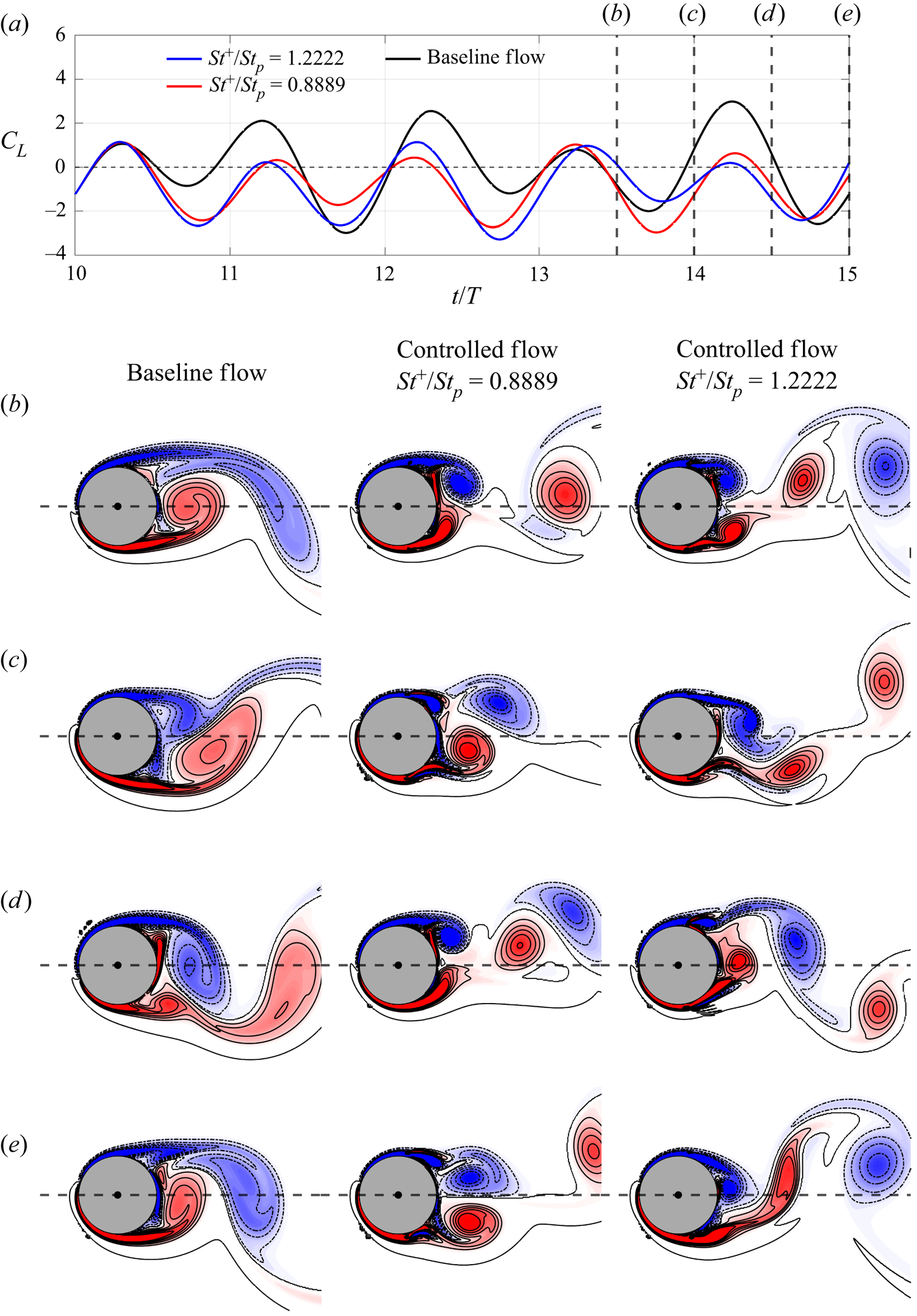
Figure 8. (a) Comparison between the lift coefficients of the baseline flow (black curve) and controlled flows with tangential actuations at  $St^+/St_p = 0.8889$ (red curve) and 1.2222 (blue curve) over the control horizon. Vorticity snapshots of the baseline flow and the controlled flows at $t/T=$ (b) 13.5, (c) 14, (d) 14.5 and (e) 15. Positive and negative vorticity contour levels are plotted respectively in solid and dash-dotted curves. The evolutions of the baseline flow and the controlled flows can be seen in the supplementary movie.
The correspondence between control efficacy and mode structures can be observed in two ways. For the traditional resolvent analysis of the LTI system, the control is expected to be most effective when the control forcing inputs (especially the internal forcing that causes the nonlinear interaction of the disturbed flow) are aligned with the rank-1 forcing mode. At the same time, the largest response in the flow is expected to be in the rank-1 response mode. Unfortunately, due to the limit of the Lyapunov–Floquet transformation, this correspondence can only be observed indirectly. First, the mode structures of the baseline flow and the controlled flows are compared. As a result of  $\boldsymbol {y}(t) = \boldsymbol{\mathsf{P}}(t)^{-1}\boldsymbol {x}(t)$, $\hat {\boldsymbol {y}}(\omega )$ can be expressed as the infinite sum of the weighted periodic replications of $\hat {\boldsymbol {x}}(\omega )$, i.e. $\hat {\boldsymbol {y}}(\omega ) = \sum _{n=-\infty }^\infty \hat {\boldsymbol{\mathsf{P}}}_n^{-1} \hat {\boldsymbol {x}}(\omega + n\omega _p)$, where $\hat {\boldsymbol{\mathsf{P}}}_n^{-1}$ are the Fourier coefficients of $\boldsymbol{\mathsf{P}}(t)^{-1}$. In figure 9, $\hat {\boldsymbol {x}}(\omega )$ near $\omega = | \omega ^* + n \omega _p|\ (St/St_p = | St^*/St_p + n|)$ with $n = 0, \pm 1$ and $\pm 2$ for the baseline flow and the controlled flows with $St^+/St_p = 0.8889$ and 1.2222 are plotted. Both the baseline flow and the controlled flows have a finer structure at a higher frequency. The structure of the baseline flow is nearly symmetric about the centreline at all the frequencies examined. For $n = 1$ and $\pm 2$, the structures of the controlled flows show only minor differences from that of the baseline flow. However, for $n=0$ (figure 9a) and $-1$ (figure 9b), actuations in both controlled flows induce a Kárman-vortex-street-like structure that qualitatively agrees with the leading resolvent response mode at $St = St^*$ (figure 5b).

Figure 9. The mode structures of the flow at  $St/St_p =$ (a) 0.4, (b) 0.6, (c) 1.4, (d) 1.6 and (e) 2.4 for the baseline flow and the controlled flows with $St^+/St_p = 0.8889$ and 1.2222. Positive and negative vorticity contour levels are plotted respectively in solid and dash-dotted curves.
Next, the mode structures of the internal forcing of the baseline flow and the controlled flows are compared. Similarly, as a result of  $\boldsymbol {G}(t) = \boldsymbol{\mathsf{P}}(t)^{-1}\boldsymbol {g}(t)$, $\hat {\boldsymbol {G}}(\omega ) = \sum _{n=-\infty }^\infty \hat {\boldsymbol{\mathsf{P}}}_n^{-1} \hat {\boldsymbol {g}}(\omega + n\omega _p)$. In figure 10, $\hat {\boldsymbol {g}}_{{int}}(\omega )$ near $\omega = | \omega ^* + n \omega _p|\ (St/St_p = | St^*/St_p + n|)$ with $n = 0,\ \pm 1$ and $\pm 2$ for the baseline flow and the controlled flows with $St^+/St_p = 0.8889$ and 1.2222 are plotted. The structure of the internal forcing of the baseline flow is nearly symmetric about the centreline and has a larger magnitude in the shear layer than in the wake except at $n = 2$. Nevertheless, the mode structures of the internal forcing of the baseline flow are mostly aligned with the leading resolvent forcing mode at $St = St^*$ (figure 5b), which is a wake-like structure. In both controlled flows, the actuations focus the internal forcing more into the wake region, where the leading resolvent forcing mode at $St = St^*$ has the largest magnitude. In particular, the controlled flow with $St^+/St_p = 0.8889$, in which in our theory the second-order interaction has been excited, can be observed to have a more compact internal forcing in the wake region than the controlled flow with $St^+/St_p = 1.2222$ that excites only the first-order interaction.

Figure 10. The mode structures of the internal forcing at  $St/St_p =$ (a) 0.4, (b) 0.6, (c) 1.4, (d) 1.6 and (e) 2.4 for the baseline flow and the controlled flows with $St^+/St_p = 0.8889$ and 1.2222. Positive and negative vorticity contour levels are plotted respectively in solid and dash-dotted curves.
5. Conclusion
In this study, a design tool for the active flow control of a plunging circular cylinder is developed by combining resolvent analysis and the Floquet theory. In order to extend the stationary-boundary-based resolvent analysis to a moving boundary, the analysis is performed in the cylinder-fixed frame, where the incompressible flow linearized about a time-averaged base flow yields a LTP system for control. The corresponding monodromy matrix, which characterizes the system dynamics after a period of the plunging motion, can be built from the simulations of the homogeneous LTP system based on the Floquet theory. Using the Lyapunouv–Floquet transformation, the LTP system is transformed into a similar LTI system, whose resolvent depends on the principal matrix logarithm of the monodromy matrix. By examining the largest singular value of the resolvent over the complex frequency plane, the resulting pseudo-spectrum reveals the existence of an optimal actuating Strouhal number of 0.1464 to excite the transformed linear system, which leads to multiple harmonic and subharmonic frequencies for effective actuations of the flow around a plunging cylinder. Simulations show that the active control is more effective with tangential actuations than normal ones in reducing the lift fluctuation of a plunging cylinder. When the flow is actuated tangentially near the predicted harmonic and subharmonic frequencies at the separation points, the lift fluctuation of a plunging cylinder can be reduced by up to 25.7 % by efficiently slowing the growth of the boundary layer and disrupting the formation of vortices in the shear layer. The modal analysis shows that the actuation results in an internal nonlinear forcing that is aligned with the leading resolvent forcing mode; while the controlled flow demonstrates the largest response that is aligned with the leading resolvent response mode as expected.
Supplementary movie
Supplementary movie is available at https://doi.org/10.1017/jfm.2023.526.
Funding
This work was supported by the Ministry of Science and Technology, Taiwan (grant numbers MOST 109-2636-E-002-018 and MOST 110-2636-E-002-022).
Declaration of interests
The authors report no conflict of interest.
Author contributions
H.-C.T. derived the theory and C.-T.L. and M.-L.T. performed the simulations. All authors contributed equally to analysing data and reaching conclusions, and in writing the paper.
Appendix A. Derivation of the harmonic resolvent from the LTI system resolvent obtained by the Lyapunov–Floquet transformation
Consider a forced  $T_0$-periodic linear system ${\textrm {d}\kern0.7pt \boldsymbol {x}}/{\textrm {d}t} = \boldsymbol{\mathsf{A}}(t)\boldsymbol {x} + \boldsymbol {g}$, where $\boldsymbol{\mathsf{A}}(t+T_0) = \boldsymbol{\mathsf{A}}(t)$. Based on the Floquet theory, the fundamental solution matrix $\boldsymbol{\mathsf{X}}(t)$ can be decomposed as the product of two matrices, $\boldsymbol{\mathsf{X}}(t) = \boldsymbol{\mathsf{P}}(t)\textrm {e}^{\boldsymbol{\mathsf{B}}t}$, where $\boldsymbol{\mathsf{P}}(t+T_0) = \boldsymbol{\mathsf{P}}(t)$ is a $T_0$-periodic matrix and $\boldsymbol{\mathsf{B}}$ is a constant matrix. Since $\boldsymbol{\mathsf{X}}(t)$ satisfies the equation ${\textrm {d}\boldsymbol{\mathsf{X}}}/{\textrm {d}t} = \boldsymbol{\mathsf{A}}(t)\boldsymbol{\mathsf{X}}$, $\boldsymbol{\mathsf{P}}(t)$ satisfies the equation
 \begin{equation} \frac{{\rm d}\boldsymbol{\mathsf{P}}}{{\rm d}t} + \boldsymbol{\mathsf{P}}\boldsymbol{\mathsf{B}} = \boldsymbol{\mathsf{A}}\boldsymbol{\mathsf{P}}. \end{equation}
Moreover, we consider the Fourier series of the periodic matrices  $[\boldsymbol{\mathsf{A}}(t),\boldsymbol{\mathsf{P}}(t)] = \sum _{n = 0}^\infty$ $[\hat {\boldsymbol{\mathsf{A}}}_n, \hat {\boldsymbol{\mathsf{P}}}_n] \textrm {e}^{-\textrm {i}n\omega _0t}$, where $n$ is an integer and $\omega _0 = 2{\rm \pi} /T_0$, then (A1) becomes
 \begin{equation} -{\rm i} n \omega_0 \hat{\boldsymbol{\mathsf{P}}}_n + \hat{\boldsymbol{\mathsf{P}}}_n\boldsymbol{\mathsf{B}} = \sum_{\alpha={-}\infty}^ \infty \hat{\boldsymbol{\mathsf{A}}}_{n-\alpha}\hat{\boldsymbol{\mathsf{P}}}_\alpha . \end{equation}
 As illustrated in §§ 3.2 and 3.3, by introducing the Lyapunov–Floquet transformation  $\boldsymbol {y}(t) = \boldsymbol{\mathsf{P}}(t)^{-1}\boldsymbol {x}(t)$ and $\boldsymbol {G}(t) = \boldsymbol{\mathsf{P}}(t)^{-1}\boldsymbol {g}(t)$, the LTI system ${\textrm {d}\boldsymbol {y}}/{\textrm {d}t} = \boldsymbol{\mathsf{B}}\boldsymbol {y} + \boldsymbol {G}$ is obtained. We can further consider the Fourier transform $[\boldsymbol {x}(t),\boldsymbol {g}(t),\boldsymbol {y}(t),\boldsymbol {G}(t)] = \int _{-\infty }^\infty [\hat {\boldsymbol {x}}(\omega ),\hat {\boldsymbol {g}}(\omega ),\hat {\boldsymbol {y}}(\omega )$, $\hat {\boldsymbol {G}}(\omega )] \textrm {e}^{-\textrm {i}\omega t} \,\textrm {d}\omega$ and express the relationship between $\boldsymbol {y}(t)$ and $\boldsymbol {G}(t)$ in frequency space as
 \begin{equation} \hat{\boldsymbol{y}}(\omega) = \left(-{\rm i}\omega \boldsymbol{\mathsf{I}} - \boldsymbol{\mathsf{B}} \right)^{{-}1} \hat{\boldsymbol{G}}(\omega) = \boldsymbol{\mathcal{H}}\left(\omega\right) \hat{\boldsymbol{G}}(\omega) , \end{equation}
where the linear operator  $\boldsymbol {\mathcal {H}}(\omega ) = (-\textrm {i}\omega \boldsymbol{\mathsf{I}} - \boldsymbol{\mathsf{B}} )^{-1}$ is the resolvent of the LTI system. Again, using the Fourier series of $\boldsymbol{\mathsf{P}}(t)$, the relationships between $\hat {\boldsymbol {x}}(\omega )$ and $\hat {\boldsymbol {y}}(\omega )$, and between $\hat {\boldsymbol {g}}(\omega )$ and $\hat {\boldsymbol {G}}(\omega )$ are
 \begin{equation} \hat{\boldsymbol{x}}(\omega) = \sum_{n ={-}\infty}^\infty \hat{\boldsymbol{\mathsf{P}}}_n \hat{\boldsymbol{y}}(\omega - n \omega_0)\quad \text{and}\quad \hat{\boldsymbol{g}}(\omega) = \sum_{n ={-}\infty}^\infty \hat{\boldsymbol{\mathsf{P}}}_n \hat{\boldsymbol{G}}(\omega - n \omega_0). \end{equation}
From (A2), (A3) and (A4a,b), it can be shown that  $\hat {\boldsymbol {x}}(\omega )$ satisfies
 \begin{equation} -{\rm i}\omega \hat{\boldsymbol{x}}(\omega) = \sum_{s={-}\infty}^ \infty \hat{\boldsymbol{\mathsf{A}}}_s\hat{\boldsymbol{x}}(\omega-s\omega_0) + \hat{\boldsymbol{g}}(\omega) , \end{equation}
which is consistent with the Fourier transform of the LTP system. From the above derivation we can see that the transformed LTI system retains the same amount of information as the LTP system. However, in real application truncation is needed in (A4a,b) to lower the computational cost of obtaining sufficiently accurate dynamics of the LTP system.
If we further assume  $\boldsymbol {x}(t)$, $\boldsymbol {g}(t)$, $\boldsymbol {y}(t)$, $\boldsymbol {G}(t)$ are formed by harmonic functions with a fundamental harmonic frequency of $\omega _0$, i.e. their spectra are formed by distinct Fourier coefiicients $[\hat {\boldsymbol {x}}(\omega ),\hat {\boldsymbol {g}}(\omega ),\hat {\boldsymbol {y}}(\omega ),\hat {\boldsymbol {G}}(\omega )] = \sum _{n=-\infty }^\infty [\hat {\boldsymbol {x}}_n,\hat {\boldsymbol {g}}_n,\hat {\boldsymbol {y}}_n,\hat {\boldsymbol {G}}_n] \delta (\omega - n\omega _0)$, then the relationships between $\hat {\boldsymbol {x}}_n$ and $\hat {\boldsymbol {y}}_n$, and between $\hat {\boldsymbol {g}}_n$ and $\hat {\boldsymbol {G}}_n$ are
 \begin{equation} \hat{\boldsymbol{x}}_n = \sum_{m ={-}\infty}^\infty \hat{\boldsymbol{\mathsf{P}}}_{n-m} \hat{\boldsymbol{y}}_m\quad \text{and}\quad \hat{\boldsymbol{g}}_n = \sum_{m ={-}\infty}^\infty \hat{\boldsymbol{\mathsf{P}}}_{n-m} \hat{\boldsymbol{G}}_m . \end{equation}
Moreover,  $\hat {\boldsymbol {x}}_n$ satisfies the equation
 \begin{equation} -{\rm i} n \omega_0 \hat{\boldsymbol{x}}_n = \sum_{m ={-}\infty}^\infty \hat{\boldsymbol{\mathsf{A}}}_{n-m}\hat{\boldsymbol{x}}_m + \hat{\boldsymbol{g}}_n , \end{equation}
which is the harmonic resolvent formulation used by Padovan et al. (Reference Padovan, Otto and Rowley2020). Therefore, when the LTP system has multiple dominant frequencies, (A7) may not be valid since  $\boldsymbol {x}(t)$ could have a different fundamental harmonic frequency from that of $\boldsymbol{\mathsf{A}}(t)$.


 Open access