


1. Introduction
Although the principal role of large-scale forcing is to sustain turbulence, it also has a profound effect on the small-scale dynamics. In most flows occurring in nature, large-scale forcing takes the form of production which extracts kinetic energy from the mean flow and injects it into the turbulent field (Tennekes & Lumley Reference Tennekes and Lumley2018; Pope Reference Pope2000). Production, which is a function of the mean velocity gradients (VGs) and Reynolds stresses, is strongly flow dependent and can be anisotropic and inhomogeneous. Numerically generated turbulence is sustained by randomised forcing at large scales (Eswaran & Pope Reference Eswaran and Pope1988). In most cases, the kinetic energy is introduced in the large scales and it subsequently cascades to smaller scales, due to the nonlinear inertial action, before being dissipated at the viscous small scales. Even though the forcing mechanism is prominent at the larger scales, it is responsible for sustaining turbulence at all scales of motion.
Kolmogorov (Reference Kolmogorov1941) proposed that at high enough Reynolds numbers, the small-scale behaviour is insensitive to the manner of large-scale forcing. In recent years some studies (Yeung & Brasseur Reference Yeung and Brasseur1991; Biferale & Vergassola Reference Biferale and Vergassola2001; Danaila, Anselmet & Antonia Reference Danaila, Anselmet and Antonia2002) have shown that anisotropic features of large-scale forcing do carry over to the small scales to some degree. Nonetheless, the small-scale universality is observed in a variety of flows with different types of forcing. As a consequence, numerical simulations of forced isotropic turbulence (FIT) have been widely used to understand small-scale characteristics such as VG structure functions and scaling exponents. Much attention has been given to the probability distribution and dynamical behaviour of second and third invariants ( $Q,R$) of the VG tensor due to their importance in classifying the local streamline topology (Chong, Perry & Cantwell Reference Chong, Perry and Cantwell1990). It is now well established that the $Q$–
$Q$– $R$ joint probability density function (p.d.f.) has a characteristic tear-drop shape in various turbulent flows subject to different types of forcing (Soria et al. Reference Soria, Sondergaard, Cantwell, Chong and Perry1994; Blackburn, Mansour & Cantwell Reference Blackburn, Mansour and Cantwell1996; Chong et al. Reference Chong, Soria, Perry, Chacin, Cantwell and Na1998; Dodd & Jofre Reference Dodd and Jofre2019). In addition, it has also been shown that the $Q$–
$Q$– $R$ conditional mean trajectories (CMTs) due to inertia, pressure and viscous mechanisms are very similar in different types of flows such as FIT, turbulent boundary layers and mixing layers. (Martín et al. Reference Martín, Ooi, Chong and Soria1998; Ooi et al. Reference Ooi, Martin, Soria and Chong1999; Chevillard et al. Reference Chevillard, Meneveau, Biferale and Toschi2008; Atkinson et al. Reference Atkinson, Chumakov, Bermejo-Moreno and Soria2012; Lawson & Dawson Reference Lawson and Dawson2015; Bechlars & Sandberg Reference Bechlars and Sandberg2017; Wu, Moreau & Sandberg Reference Wu, Moreau and Sandberg2019). To date, the role of large-scale production (or random forcing) in small-scale dynamics has not been established. Lacking such understanding, our knowledge of turbulence small scales must be considered incomplete.
The objective of this study is to examine the role of large-scale forcing in VG dynamics. Specifically, we seek to establish the interplay between forcing, inertial, pressure and viscous mechanisms that leads to the ‘universal’ features of VGs, such as the tear-drop shape of the  $Q$–
$Q$– $R$ joint p.d.f. and near-log-normal distribution of the pseudo-dissipation (Obukhov Reference Obukhov1962; Yeung & Pope Reference Yeung and Pope1989). While the $Q$–
$Q$– $R$ phase plane accurately classifies the local streamlines into four distinct topologies, it cannot uniquely determine the streamline geometry (Elsinga & Marusic Reference Elsinga and Marusic2010; Das & Girimaji Reference Das and Girimaji2020). Further, $Q,R$ values can grow without bounds with increasing Reynolds numbers. It is pointed out by Girimaji & Speziale (Reference Girimaji and Speziale1995) that VG tensor normalised by its magnitude (Frobenius norm) is better suited for examining many aspects of small-scale dynamics. Specifically, the normalised invariants ( $q,r$) provide a bounded phase-space that uniquely characterises the complete shape of the local flow streamlines (Das & Girimaji Reference Das and Girimaji2019, Reference Das and Girimaji2020). In this study, we first demonstrate that the $q$–
$q$– $r$ p.d.f. exhibits a greater degree of self-similarity over different flows than $Q$–
$Q$– $R$ p.d.f. The inertial, pressure and viscous action in the compact $q$–
$q$– $r$ plane constitutes a well-defined but incomplete dynamical system and yet yields important insight into the nature of these turbulence processes (Das & Girimaji Reference Das and Girimaji2020). To complete the description of VG dynamics, the effect of forcing is examined in the normalised $q$–
$q$– $r$ framework. In the following section, we present a thorough investigation into the effect of inertia, pressure, viscosity and large-scale forcing on the evolution of the VG magnitude.
Toward this end, we first derive the governing equations for the normalised VG tensor and the VG magnitude highlighting the contribution of the forcing term. We develop the p.d.f. evolution equations for the normalised invariants,  $q$ and $r$, as well as the VG magnitude, $A$, in § 2. Analysis of the direct numerical simulation (DNS) data and a discussion of the findings are given in §§ 3–6. The final conclusions are presented in § 7.
2. Forcing in VG evolution equations
The governing Navier–Stokes equations for velocity fluctuations,  $u_i$, as obtained from the mass and momentum conservation of an incompressible flow are given by
 $$\begin{gather} \frac{\partial u_i}{\partial t} + u_k\frac{\partial u_i}{\partial x_k} ={-} \frac{\partial p}{\partial x_i} + \nu \nabla^{2} u_i + f_i , \end{gather}$$
 $$\begin{gather}\frac{\partial u_i}{\partial x_i}= 0 , \end{gather}$$
where  $p$ is the pressure fluctuation, $\nu$ is the kinematic viscosity and $f_i$ represents forcing. The pressure and viscous terms represent important non-local effects on the evolution of the velocity field. The forcing term is responsible for the production of energy at the large scales, which compensates for the viscous dissipation of energy at the smaller scales. The general form of forcing encountered in most turbulent flows is
 \begin{equation} f_i ={-} \langle U_k \rangle \frac{\partial u_i}{\partial x_k} - u_k \frac{\partial \langle U_i \rangle}{\partial x_k} + \frac{\partial}{\partial x_k} \langle u_i u_k \rangle, \end{equation}
where  $U_i = \langle U_i \rangle + u_i$ is the total velocity. Here $\langle. \rangle$ indicates ensemble averaging or spatial averaging in the homogeneous directions. The forcing depends on the mean flow field and inhomogeneity of turbulent fluctuations (Rogallo Reference Rogallo1981; Rogers & Moin Reference Rogers and Moin1987; Lee & Moser Reference Lee and Moser2015; Quadrio, Frohnapfel & Hasegawa Reference Quadrio, Frohnapfel and Hasegawa2016). Forcing in a numerical simulation of homogeneous isotropic turbulence with no mean flow ( $\langle U_i \rangle =0$) entails injecting energy into the lowest-wavenumber shells. This forcing is a function of time and space and can be of different types (Eswaran & Pope Reference Eswaran and Pope1988; Machiels Reference Machiels1997; Overholt & Pope Reference Overholt and Pope1998; Donzis & Yeung Reference Donzis and Yeung2010).
We examine the effect of forcing on the evolution of the VG tensor,
 \begin{equation} A_{ij} = \frac{\partial u_i}{\partial x_j} \quad \text{where}\ A_{ii} = 0. \end{equation}
From (2.1a), the evolution equation for VG tensor  $A_{ij}$ can be derived:
 \begin{equation} \frac{\partial A_{ij}}{\partial t} + u_k \frac{\partial A_{ij}}{\partial x_k} ={-} A_{ik} A_{kj} - \frac{\partial^{2} p}{\partial x_i \partial x_j} + \nu \nabla^{2} A_{ij} + \frac{\partial f_i}{\partial x_j}. \end{equation}
Here,  $(-A_{ik}A_{kj})$ is referred to as the inertial term, which includes vortex stretching and strain self-amplification. Using the incompressibility condition ( $A_{ii}=0$) in (2.4), it can be shown that
 \begin{equation} {-}\frac{\partial^{2} p}{\partial x_i \partial x_i} + \frac{\partial f_i}{\partial x_i} = A_{ik} A_{ki}. \end{equation}
Note that the second term is zero in FIT because  $f_i$ is a solenoidal field by construction. Applying (2.5), the VG tensor evolution equation (2.4) can be written as
 \begin{equation} \frac{{\rm d}A_{ij}}{{\rm d}t} ={-} A_{ik}A_{kj} + \frac{1}{3} A_{mk}A_{km} \delta_{ij} + H_{ij} + V_{ij} + G_{ij} , \end{equation}
where  ${\rm d}/{\rm d}t = \partial /\partial t + u_k \partial /\partial x_k$ is material or substantial derivative. Here, $\boldsymbol {H}$ is the anisotropic pressure Hessian tensor, $\boldsymbol {V}$ is the viscous Laplacian tensor and $\boldsymbol {G}$ is the anisotropic forcing tensor, defined as follows:
 \begin{equation} H_{ij} ={-} \frac{\partial^{2} p}{\partial x_i \partial x_j} + \frac{\partial^{2} p}{\partial x_k \partial x_k} \frac{\delta_{ij}}{3} ;\quad V_{ij} = \nu \nabla^{2} A_{ij} ; \quad G_{ij} = \frac{\partial f_i}{\partial x_j} - \frac{\partial f_k}{\partial x_k}\frac{\delta_{ij}}{3} . \end{equation}
The anisotropic forcing tensor  $G_{ij}$ represents the influence of the mean flow and inhomogeneity on the fluctuating VG evolution. In the case of FIT, $G_{ij}$ represents the effect of artificial large scale forcing on the fluctuating field.
Following Girimaji & Speziale (Reference Girimaji and Speziale1995) and Das & Girimaji (Reference Das and Girimaji2019),  $A_{ij}$ is factorised into VG magnitude $A$ and a normalised VG tensor ( $b_{ij}$):
 \begin{equation} b_{ij} \equiv \frac{A_{ij}}{A} \quad \text{where} \ A\equiv \|\boldsymbol{A}\|_F=\sqrt{A_{ij}A_{ij}}. \end{equation}
Here,  $\|.\|_F$ is the Frobenius norm of the tensor. All of the information about the geometry of the local streamline structure of the flow is contained within the mathematically bounded tensor $b_{ij}$ (Das & Girimaji Reference Das and Girimaji2020). Furthermore, the topological classification of the local flow streamlines (Chong et al. Reference Chong, Perry and Cantwell1990) can also be described in the bounded phase plane of $b_{ij}$ invariants, $q$ and $r$:
$r$:
 \begin{equation} q ={-}\tfrac{1}{2} b_{ij} b_{ji} ;\quad r ={-} \tfrac{1}{3} b_{ij} b_{jk} b_{ki}. \end{equation}
The VG magnitude  $A$, on the other hand, determines the scale factor of the local flow streamlines. In this work, we examine the effect of forcing on $A$ and $b_{ij}$ individually.
2.1. Evolution equations of normalised VG tensor
Using (2.6) and (2.8), we can derive the following evolution equation for  $b_{ij}$:
 \begin{align} \frac{{\rm d} b_{ij}}{{\rm d} t'} &={-} b_{ik}b_{kj} + \frac{1}{3} b_{km} b_{mk} \delta_{ij} + b_{ij} b_{mk} b_{kn} b_{mn} + (h_{ij} - b_{ij} b_{kl} h_{kl}) \nonumber\\ &\quad + (v_{ij} - b_{ij} b_{kl} v_{kl}) + (g_{ij} - b_{ij} b_{kl} g_{kl}), \end{align}
where  ${\rm d}t'=A\,{\rm d}t$ represents a normalised time increment and
 \begin{equation} h_{ij} = \frac{H_{ij}}{A^{2}} ;\quad v_{ij} = \frac{V_{ij}}{A^{2}} ;\quad g_{ij} = \frac{G_{ij}}{A^{2}} \end{equation}
are the normalised anisotropic pressure Hessian, viscous Laplacian and anisotropic forcing tensors, respectively. Similarly, the following governing equations for  $q$ and $r$ can be derived (Das & Girimaji Reference Das and Girimaji2019) from (2.10):
 $$\begin{gather} \frac{{\rm d} q}{{\rm d} t'} ={-} 3 r + 2 q b_{ij} b_{ik} b_{kj} - h_{ij}(b_{ji} + 2qb_{ij}) - v_{ij}(b_{ji} + 2qb_{ij}) - g_{ij}(b_{ji} + 2qb_{ij}) , \end{gather}$$
 $$\begin{gather}\frac{{\rm d} r}{{\rm d} t'} = \frac{2}{3} q^{2} + 3 r b_{ij} b_{ik} b_{kj} - h_{ij}(b_{jk}b_{ki} + 3rb_{ij}) - v_{ij}(b_{jk}b_{ki} + 3rb_{ij}) - g_{ij}(b_{jk}b_{ki} + 3rb_{ij}) . \end{gather}$$
The first two terms on the right-hand side of (2.12)–(2.13) are referred to as the nonlinear ( $N$) terms that constitute the inertial and isotropic pressure effects in a turbulent flow. The third term on the right-hand side represents anisotropic pressure effect ( $P$) whereas the fourth term embodies viscous action ( $V$) on the $q$–
$q$– $r$ dynamics. Finally, the last term in both equations represents the effect of forcing ( $F$) on the evolution of $q$ and $r$.
$r$.
2.1.1.  $b_{ij}$-p.d.f. evolution equation

Following the methodology of Girimaji & Pope (Reference Girimaji and Pope1990), the governing differential equation for the joint p.d.f. of  $b_{ij}$, $\mathcal {P}(\boldsymbol {b})$, is given by
 \begin{equation} \frac{{\rm d}\mathcal{P}}{{\rm d}t'} ={-} \frac{{\rm d}}{{\rm d}b_{ij}} \left( \mathcal{P} \left \langle \left.\frac{{\rm d}b_{ij}}{{\rm d}t'} \right| \boldsymbol{b} \right \rangle \right). \end{equation}
Here, the  ${{\rm d}b_{ij}}/{{\rm d}t'}$ is given by (2.10). In this work, we restrict our analysis to the $\boldsymbol {b}$ invariants, $q$ and $r$. The evolution equation for the $q$–
$q$– $r$ joint p.d.f., $\mathcal {F}(q,r)$, is given by
 \begin{equation} \frac{{\rm d}\mathcal{F}}{{\rm d}t'} ={-} \frac{{\rm d}}{{\rm d}q} \left( \mathcal{F} \left \langle \left.\frac{{\rm d}q}{{\rm d}t'} \right | q,r \right\rangle \right) - \frac{{\rm d}}{{\rm d}r} \left( \mathcal{F} \left\langle \left.\frac{{\rm d}r}{{\rm d}t'} \right| q,r \right\rangle \right). \end{equation}
The above conditional average terms are composed of the effects of nonlinear, pressure, viscous and forcing processes from (2.12)–(2.13).
2.1.2. Conditional mean velocity
The dynamics of the VG invariants,  $q$ and $r$, is commonly investigated by examining the CMTs (Martín et al. Reference Martín, Ooi, Chong and Soria1998). The CMTs are obtained by integrating a vector field of conditional mean velocity ( $\boldsymbol {v}$) in the $q$–
$q$– $r$ plane, given by
 \begin{equation} \boldsymbol{v} = \left\langle \left.\begin{pmatrix} {\rm d}q/{\rm d}t'\\ {\rm d}r/{\rm d}t' \end{pmatrix} \right| q,r \right\rangle . \end{equation}
2.1.3. Probability current
The probability current,  $\boldsymbol {W}$, is the p.d.f.-weighted conditional mean velocity (van der Bos et al. Reference van der Bos, Tao, Meneveau and Katz2002; Chevillard et al. Reference Chevillard, Meneveau, Biferale and Toschi2008):
 \begin{equation} \boldsymbol{W} = \mathcal{F} \boldsymbol{v} = \mathcal{F}(q,r) \times \left\langle \left.\begin{pmatrix} {\rm d}q/{\rm d}t'\\ {\rm d}r/{\rm d}t' \end{pmatrix} \right| q,r \right\rangle. \end{equation}
The evolution equation of  $q$–
$q$– $r$ joint p.d.f. (2.15) can therefore be written as
 \begin{equation} \frac{{\rm d} \mathcal{F}}{{\rm d} t'} + \boldsymbol{\nabla}\boldsymbol{\cdot} \boldsymbol{W} = 0 . \end{equation}
The divergence of  $\boldsymbol {W}$ determines the evolution rate of the p.d.f., $\mathcal {F}(q,r)$, at a given point in the $q$–
$q$– $r$ space. Probability current has identical trajectories as the CMTs, because $\boldsymbol {W}$ is obtained by multiplying $\boldsymbol {v}$ with a non-negative function $\mathcal {F}(q,r)$. The difference between the two is only in the speed of these trajectories. Probability current is used to examine the mean $q$–
$q$– $r$ evolution in this study owing to its inherent physical relevance. The $q$–
$q$– $r$ probability currents due to nonlinear ( $N$), anisotropic pressure ( $P$), viscous ( $V$) and forcing ( $F$) effects can be defined individually as follows, from (2.12)–(2.13) and (2.17):
 \begin{equation} \left.\begin{gathered} \boldsymbol{W}_N = \mathcal{F} \left\langle \left.\begin{pmatrix} - 3 r + 2 q b_{ij} b_{ik} b_{kj} \\ \frac{2}{3} q^{2} + 3 r b_{ij} b_{ik} b_{kj} \end{pmatrix} \right| q,r \right\rangle ; \\ \boldsymbol{W}_P = \mathcal{F} \left \langle \left.\begin{pmatrix} - h_{ij}(b_{ji} + 2qb_{ij}) \\ - h_{ij}(b_{jk}b_{ki} + 3rb_{ij}) \end{pmatrix} \right| q,r \right\rangle ; \\ \boldsymbol{W}_V = \mathcal{F} \left \langle \left.\begin{pmatrix} - v_{ij}(b_{ji} + 2qb_{ij}) \\ - v_{ij}(b_{jk}b_{ki} + 3rb_{ij}) \end{pmatrix} \right| q,r \right \rangle ; \\ \boldsymbol{W}_F = \mathcal{F} \left \langle \left.\begin{pmatrix} - g_{ij}(b_{ji} + 2qb_{ij}) \\ - g_{ij}(b_{jk}b_{ki} + 3rb_{ij}) \end{pmatrix} \right| q,r \right\rangle . \end{gathered}\right\}\end{equation}
2.1.4. Statistically stationary homogeneous flow
The  $q$–
$q$– $r$ p.d.f. (2.18) for a statistically steady and homogeneous turbulent flow leads to
 \begin{equation} \frac{{\rm d} \mathcal{F}}{{\rm d} t'} = \frac{\partial \mathcal{F}}{\partial t'} ={-} \boldsymbol{\nabla} \boldsymbol{\cdot} \boldsymbol{W} ={-}\boldsymbol{\nabla}\boldsymbol{\cdot} (\boldsymbol{W}_N + \boldsymbol{W}_P + \boldsymbol{W}_V +\boldsymbol{W}_F) = 0. \end{equation}
Most studies in the past (Martín et al. Reference Martín, Ooi, Chong and Soria1998; Ooi et al. Reference Ooi, Martin, Soria and Chong1999; Chevillard et al. Reference Chevillard, Meneveau, Biferale and Toschi2008; Atkinson et al. Reference Atkinson, Chumakov, Bermejo-Moreno and Soria2012) have examined only the nonlinear, pressure and viscous effects. From DNS data presented in these studies,  $\boldsymbol {\nabla }\boldsymbol {\cdot }(\boldsymbol {W}_N + \boldsymbol {W}_P + \boldsymbol {W}_V) \neq 0$ and correspondingly the CMTs or probability currents given by $(\boldsymbol {W}_N + \boldsymbol {W}_P + \boldsymbol {W}_V)$ do not form closed-loop orbits. Clearly, in order for $\boldsymbol {\nabla }\boldsymbol {\cdot }\boldsymbol {W} = 0$, the contribution of the forcing terms is critically important. This must also render the CMTs to form closed loops.
2.2. Evolution equations of VG magnitude
The dynamics of VG magnitude ( $A$) is examined in terms of
 \begin{equation} \theta \equiv \ln A. \end{equation}
The evolution equation for  $\theta$, as derived from (2.6), is
 \begin{equation} \frac{{\rm d} \theta}{{\rm d} t^{*}} = \frac{1}{\langle A \rangle} (- b_{ik}b_{kj}A_{ij} + h_{ij}A_{ij} + v_{ij}A_{ij} + g_{ij}A_{ij}) ; \quad t^{*} = \langle A \rangle t \end{equation}
Here,  $t^{*}$ is time normalised by the global mean of VG magnitude. We choose to consider $\theta$ evolution in $t^{*}$ timescale which is the same for all fluid particles in the flow. Here, the four terms on the right-hand side of the above equation represent the nonlinear ( $N$), pressure ( $P$), viscous ( $V$) and forcing ( $F$) effects on VG magnitude evolution.
2.2.1. $\theta$-p.d.f. evolution equation

The governing differential equation for the p.d.f. of  $\theta$, $\tilde {f}(\theta )$, is given by (Pope Reference Pope1985)
 \begin{equation} \frac{{\rm d} \tilde{f}}{{\rm d}t^{*}} ={-} \frac{{\rm d}}{{\rm d}\theta} \left(\tilde{f} \left\langle \left.\frac{{\rm d}\theta}{{\rm d}t^{*}}\right| \theta \right\rangle \right). \end{equation}
2.2.2. Conditional mean rate of change
The VG magnitude dynamics is examined in terms of the mean rate of change of  $\theta$ conditioned on $\theta$,
 \begin{equation} \tilde{u} = \left \langle \left.\frac{{\rm d}\theta}{{\rm d}t^{*}} \right| \theta \right \rangle = \tilde{u}_N + \tilde{u}_P + \tilde{u}_V + \tilde{u}_F, \end{equation}
where
 \begin{equation} \left.\begin{gathered} \tilde{u}_N = \frac{1}{\langle A \rangle} \left \langle \left.- b_{ik} b_{kj} A_{ij} \right | \theta \right \rangle ;\quad \tilde{u}_P = \frac{1}{\langle A \rangle} \left \langle \left.- h_{ij} A_{ij} \right| \theta \right\rangle ;\\ \tilde{u}_V = \frac{1}{\langle A \rangle} \left\langle \left. - v_{ij} A_{ij} \right| \theta \right\rangle ; \quad \tilde{u}_F = \frac{1}{\langle A \rangle} \left\langle \left. - g_{ij} A_{ij} \right| \theta \right \rangle \end{gathered}\right\}\end{equation}
represent the mean nonlinear, pressure, viscous and forcing effects. For a statistically stationary homogeneous turbulent flow, equation (2.23) can now be written as
 \begin{equation} \frac{{\rm d} \tilde{f}}{{\rm d}t^{*}} = \frac{\partial \tilde{f}}{\partial t^{*}} ={-} \frac{\partial}{\partial\theta} [\tilde{f} (\tilde{u}_N + \tilde{u}_P + \tilde{u}_V + \tilde{u}_F) ]= 0. \end{equation}
Therefore, for the p.d.f.  $\tilde {f}(\theta )$ to be stationary, the sum of the p.d.f.-weighted conditional mean contributions of all the processes should not be a function of $\theta$ and indeed be zero as the flux vanishes at the integration boundaries.
3. Numerical simulation data
Established DNS data sets of FIT and turbulent channel flow at high Reynolds numbers are used for analysis in this study. The FIT data from the Johns Hopkins Turbulence Database (Perlman et al. Reference Perlman, Burns, Li and Meneveau2007; Li et al. Reference Li, Perlman, Wan, Yang, Meneveau, Burns, Chen, Szalay and Eyink2008) have been widely used for investigating VG statistics (Johnson & Meneveau Reference Johnson and Meneveau2016; Elsinga et al. Reference Elsinga, Ishihara, Goudar, Da Silva and Hunt2017; Danish & Meneveau Reference Danish and Meneveau2018) as well as its Lagrangian dynamics (Yu & Meneveau Reference Yu and Meneveau2010a,Reference Yu and Meneveaub) in turbulence. The data used in the present study are obtained from computations performed on a  $1024^{3}$ grid using a pseudo-spectral solver. The large-scale forcing in the flow is effected by energy injection keeping the total energy constant in lowest wavenumber modes of magnitude ${\leqslant }2$. The Taylor Reynolds number is
 \begin{equation} Re_\lambda \equiv \frac{u'\lambda}{\nu} = 427 , \quad \text{where} \ \lambda = \sqrt{15\nu u'^{2}/\epsilon}. \end{equation}
Here,  $\lambda$ is the Taylor microscale, $u'$ is the root-mean-square velocity and $\epsilon = 2\nu \langle S_{ij} S_{ij} \rangle$ is the mean dissipation rate. The simulation is well resolved with $k_{max} \eta = 1.39$, where $k_{max}$ is the highest wavenumber resolved and $\eta$ is the Kolmogorov's length scale. Field velocity data at multiple consecutive time steps, separated by $\Delta t = 0.0002 \approx 0.005 \tau _\eta$ ( $\tau _\eta$ is Kolmogorov timescale), are used to compute the temporal derivatives.
Four FIT data sets from the Turbulence and Advanced Computations Laboratory (Donzis, Yeung & Sreenivasan Reference Donzis, Yeung and Sreenivasan2008; Yakhot & Donzis Reference Yakhot and Donzis2017) at Texas A&M University are also used. The Taylor Reynolds numbers and corresponding grid sizes of these simulations are  $Re_\lambda = 86$ $(256^{3})$, $225$
$225$  $(512^{3})$, $385$
$385$  $(1024^{3})$ and $588$
$588$  $(2048^{3})$. The resolution levels of these data sets are $k_{max} \eta = 2.83$, $1.34$, $1.41$ and $1.39$, respectively. These data sets have been used in past studies to examine higher-order statistics, intermittency and Reynolds number scaling of VGs (Donzis et al. Reference Donzis, Yeung and Sreenivasan2008; Donzis & Sreenivasan Reference Donzis and Sreenivasan2010; Yakhot & Donzis Reference Yakhot and Donzis2017; Das & Girimaji Reference Das and Girimaji2019).
Turbulent channel flow data are also taken from the Johns Hopkins Turbulence Database (Li et al. Reference Li, Perlman, Wan, Yang, Meneveau, Burns, Chen, Szalay and Eyink2008; Lee & Moser Reference Lee and Moser2015). The turbulent flow inside the channel is simulated on a  $10{\,}240 \times 1536 \times 7680$ grid with a spatially uniform pressure gradient varying in time to ensure a constant mass flux through the channel. The data set used in the computations here is obtained after statistical stationarity is achieved. The friction velocity Reynolds number of the channel flow is
 \begin{equation} Re_\tau \equiv \frac{u_\tau h}{\nu} = 5186, \end{equation}
where  $u_\tau$ is the friction velocity and $h$ is the channel half-height. The velocity field is homogeneous in the stream-wise ( $x$) and span-wise ( $z$) directions and inhomogeneous in the wall-normal ( $y$) direction. As suggested in the work of Lozano-Durán, Holzner & Jiménez (Reference Lozano-Durán, Holzner and Jiménez2015), integrating over a statistically inhomogeneous region can considerably bias the Lagrangian statistics. Therefore, to circumvent averaging over statistically inhomogeneous wall-normal ( $y$) direction, we use data at specific $y^{+}$ planes: $y^{+}=100$ ( ${Re_{\lambda }}=81$), $y^{+}=203$ ( ${Re_{\lambda }}=110$), $y^{+}=302$ ( ${Re_{\lambda }}=132$) and $y^{+}=852$ ( ${Re_{\lambda }}=183$). Data from multiple time instants are considered to achieve adequate sampling.
4. Normalised VG tensor dynamics
The large-scale forcing mechanisms are very different in homogeneous isotropic turbulence and inhomogeneous anisotropic turbulent channel flow, as outlined in § 2. In this section, we first investigate the effect of the different types of forcing on the probability distribution of the invariants of the normalised VG tensor. Then, we proceed to examine the nonlinear, pressure and viscous contributions to the evolution of the invariants in these flows. All the reported statistics are obtained using data at a given time instant in the FIT cases. On the other hand, for the channel flow case, planar data from two sufficiently separated time steps are used to determine the statistics.
The isocontour lines of the  $q$–
$q$– $r$ joint p.d.f. in forced isotropic turbulent flows at different ${Re_{\lambda }}$ and turbulent channel flow at different $y^{+}$ planes, are plotted in figure 1. The solid black lines in the third and fourth quadrants of the $q$–
$q$– $r$ plane mark the lines of zero discriminant: $d=q^{3} + (27/4)r^{2} =0$. The $q$–
$q$– $r$ plane above the discriminant lines represents focal/spiralling topologies of local flow streamlines: stable focus stretching (SFS) and unstable focus compression (UFC). The $q$–
$q$– $r$ plane below the discriminant lines mark nodal/hyperbolic streamlines with node–saddle combinations: stable-node/saddle/saddle (SN/S/S) and unstable-node/saddle/saddle (UN/S/S) (Chong et al. Reference Chong, Perry and Cantwell1990; Das & Girimaji Reference Das and Girimaji2020). Topologies to the left of $r=0$ axis are stable or converging, whereas those to the right are unstable or diverging. The $q$–
$q$– $r$ joint p.d.f.s for isotropic turbulent flow at ${Re_{\lambda }}=225$, 385, 427 and $588$ have the characteristic teardrop shape with a high probability of occurrence along the right discriminant line or Vieillefosse tail (Vieillefosse Reference Vieillefosse1984). It is evident that the p.d.f. is nearly invariant at high enough ${Re_{\lambda }}$. The $q$–
$q$– $r$ joint p.d.f.s for turbulent channel flow at different $y^{+}$ locations, corresponding to ${Re_{\lambda }}=81$, 110, 132 and $183$, are shown in figure 1(b). In this case, the p.d.f. shows slight dependence on Reynolds number. As ${Re_{\lambda }}$ increases, the isocontour lines in the focal topologies shrink closer toward the $q$-axis and the isocontour lines near the tail of the teardrop widen. The observed behaviour could be either due to the difference in Reynolds number or the wall-normal inhomogeneity in the channel flow case.

Figure 1. Isocontours of  $q$–
$q$– $r$ joint p.d.f., $\mathcal {F}(q,r)$, for (a) FIT and (b) turbulent channel flow, at different ${Re_{\lambda }}$. The highest p.d.f. level contour is along the right discriminant line and the p.d.f. level drops with distance from the line. Solid black lines in the third and fourth quadrants represent the zero-discriminant lines (Cantwell Reference Cantwell1992).
The  $q$–
$q$– $r$ p.d.f.s of FIT at ${Re_{\lambda }}=225$ and turbulent channel flow at ${Re_{\lambda }}=183$, are compared in figure 2. It is evident that in the densely populated regions of the plane, the p.d.f. values are nearly identical. There is a small difference between the p.d.f. isocontours only in the low-probability regions of the SN/S/S topology. Thus, despite having different forms of large-scale forcing, the joint probability distribution of normalised VG invariants are nearly identical in both the flows, even at moderately high Reynolds numbers. It is reasonable then to expect the overall VG dynamics to be statistically similar in both cases. To examine this further, we now investigate probability currents.

Figure 2. Isocontours of  $q$–
$q$– $r$ joint p.d.f., $\mathcal {F}(q,r)$, of FIT at ${Re_{\lambda }}=225$ (blue solid line) and turbulent channel flow at $Re_\lambda =183$ (red dashed line).
4.1. Nonlinear, pressure and viscous effects
The  $q$–
$q$– $r$ probability currents given in (2.19) represent the dynamical effects of the constituent mechanisms. The probability current of the nonlinear (inertial and isotropic pressure) effect ( $\boldsymbol {W}_N$) is plotted in figure 3 for isotropic turbulent flow and turbulent channel flow. The background colour contours represent the magnitude of $\boldsymbol {W}_{N}$, that is, the speed of the trajectories. The nonlinear effect (Cantwell Reference Cantwell1992; Bikkani & Girimaji Reference Bikkani and Girimaji2007) take trajectories from the left toward the right bottom corner along the zero-discriminant line. These probability currents are invariant with ${Re_{\lambda }}$ and identical in different types of flows, due to the fact that $\boldsymbol {W}_N$ (2.19) is fully determined by $b_{ij}$.

Figure 3. The  $q$–
$q$– $r$ probability current due to nonlinear terms ( $\boldsymbol {W}_{N}$) for (a) FIT ${Re_{\lambda }} =225$ and (b) turbulent channel flow ${Re_{\lambda }}=183$. The background contours represent the magnitude of the vector $\boldsymbol {W}_N$.
Next, the probability current due to the anisotropic pressure ( $\boldsymbol {W}_P$), is illustrated in figure 4. The currents exhibit slight variations at low ${Re_{\lambda }}$ and are nearly invariant at higher ${Re_{\lambda }}$. Only high- ${Re_{\lambda }}$ cases for both isotropic turbulence and channel flow are plotted. The principal action of the anisotropic pressure is to oppose the nonlinear current ( $\boldsymbol {W}_N$) in the majority of the $q$–
$q$– $r$ plane, except in the middle UFC region where $\boldsymbol {W}_P$ is nearly aligned with $\boldsymbol {W}_N$. The pressure probability currents repel trajectories away from the top right UFC region and attract them toward the bottom left corner of the plane, which is the repeller of the $\boldsymbol {W}_N$ field. The effect of non-local pressure is stronger in the UN/S/S topology region below the right discriminant line and in the rotation-dominated SFS region. The contribution of $\boldsymbol {W}_P$ is nearly identical in FIT and channel flow. The results clearly suggest that the effect of pressure on $q$–
$q$– $r$ dynamics is reasonably independent of large-scale forcing.

Figure 4. The  $q$–
$q$– $r$ probability current due to anisotropic pressure ( $\boldsymbol {W}_{P}$) for (a) FIT ${Re_{\lambda }} =225$ and (b) turbulent channel flow ${Re_{\lambda }} =183$. The background contours represent the magnitude of the vector $\boldsymbol {W}_P$.
The effect of viscosity in the unnormalised invariants  $Q$–
$Q$– $R$ plane depicts the damping nature of viscosity reducing the VG magnitude, as discussed in detail in Das & Girimaji (Reference Das and Girimaji2020). Further information (damping coefficients at different geometries) is revealed when we investigate the viscous effects on the dynamics of normalised invariants $q$–
$q$– $r$ (local streamline shape) and magnitude $\theta$ individually. The viscous probability currents of ${Re_{\lambda }} =225$ of FIT and ${Re_{\lambda }} =132$ of turbulent channel flow are plotted in figure 5 to illustrate the general behaviour. Expectedly, the $q$–
$q$– $r$ probability currents due to the viscous effects ( $\boldsymbol {W}_V$) show some dependence on ${Re_{\lambda }}$ in both isotropic turbulence as well as turbulent channel flow. The viscous probability current in FIT has a repeller in the lower middle UFC region and takes all trajectories toward pure-strain geometry ( $q=-1/2$ line). In turbulent channel flow, the viscous currents drive trajectories from origin and right discriminant line toward the pure-strain attractor. The viscous effects are strongest in the unstable nodal topologies below the right discriminant line. Although most features are similar in both the flows, there are minor differences, particularly in the precise location of the repeller in the phase space. This is possibly due to the differences in Reynolds number and numerical resolution in the two cases. In addition, the derivatives in FIT are computed using spectral methods, whereas the derivatives in the wall-normal direction of the channel are computed using finite-difference scheme of a lower accuracy.

Figure 5. The  $q$–
$q$– $r$ probability current due to viscous effects ( $\boldsymbol {W}_{V}$) for (a) FIT ${Re_{\lambda }} =225$ and (b) turbulent channel flow ${Re_{\lambda }} =132$. The background contours represent the magnitude of the vector $\boldsymbol {W}_V$.
Although the viscous probability current has a slight dependence on  ${Re_{\lambda }}$, it is significantly smaller in magnitude than the inertial and pressure contributions. As a result, the aggregate of the nonlinear ( $N$), anisotropic pressure ( $P$) and viscous ( $V$) contributions, represented by the subscript ‘ $NPV$’ is nearly self-similar at high enough ${Re_{\lambda }}$ in both flows as shown in figure 6. Thus, two different types of large-scale forcing lead to similar VG statistical evolution due to inertia, pressure and viscosity.

Figure 6. The  $q$–
$q$– $r$ probability currents due to nonlinear, pressure and viscous effects, $\boldsymbol {W}_{NPV}$, for (a) FIT at ${Re_{\lambda }}=427$ and (b) turbulent channel flow at ${Re_{\lambda }}=132$. The background contours represent the magnitude of the vector $\boldsymbol {W}_{NPV}$. The white dash-dotted lines represent the separatrices.
The nonlinear inertial effects lead the trajectories from the left to the right of the  $q$–
$q$– $r$ plane with the attractor located at the lower right-hand corner of the map (figure 3). The attractor of the pressure effect, on the other hand, is located on the lower left-hand corner (figure 4) and pressure causes trajectories to move from right- to left-hand side of the map. As shown in Das & Girimaji (Reference Das and Girimaji2020), the combined effect of nonlinear and pressure contributions renders all trajectories spiraling toward the origin. The origin, representing pure shear streamlines, is the attractor of this system. This pure shear attractor also appears in the phase space for the aggregate of nonlinear, pressure and viscous effects (figure 6). Its basin of attraction is surrounded by a separatrix loop, marked by the white dash-dotted line in the figure. The $q,r$ values outside the separatrix loop evolve toward the $q=-1/2$ line, which represents pure strain streamlines. The trajectories move the fastest in the unstable focal topologies and slow down significantly near the right discriminant line and at the top of the spirals. Overall, the evolution of $q,r$ due to all the turbulence processes excluding large-scale forcing does not form closed-loop trajectories. Unclosed trajectories represent a system where the $q$–
$q$– $r$ p.d.f. is not stationary in time (Lozano-Durán et al. Reference Lozano-Durán, Holzner and Jiménez2015).
The findings thus far from FIT and channel flow can be summarised as follows: (i) both are statistically steady flows with stationary  $q$–
$q$– $r$ joint p.d.f.; (ii) their $q$–
$q$– $r$ joint p.d.f.s are nearly identical; and (iii) the evolution of $q$–
$q$– $r$ joint p.d.f. due to nonlinear–pressure–viscous contributions are nearly identical, but do not form closed-loop trajectories. It is reasonable to deduce that the missing effect of large-scale forcing is key in establishing closed-loop trajectories in statistically stationary turbulence. It can also be inferred that the contribution of forcing is very similar in both the flows. In the remainder of the study, we analyse only FIT to examine and understand the effect of forcing on VG dynamics.
4.2. Forcing effects
Direct computation of the forcing term is rendered difficult due to the fact that force field is not archived in most data sets. To identify and isolate the effect of forcing on the evolution of  $q$–
$q$– $r$ we follow a three-step procedure.
(i) Determine the total rate of change (material derivatives) of
$q$ and $r$ by calculating the following:
(4.1a,b)A recent study by Lozano-Durán et al. (Reference Lozano-Durán, Holzner and Jiménez2015) has shown that computing the material derivatives of VG invariants is highly prone to numerical errors from both spatial and temporal differentiation. Inaccurate computations of these derivatives can lead to deformed CMTs. We follow the guidelines suggested in their work for accurate computation of CMTs. The spatial derivatives are computed on a two-times dealiased grid, that is, expanding the number of modes by a factor of two in all three directions. The temporal derivatives are computed using a fourth-order central difference scheme with a CFL of\begin{equation} \frac{{\rm d}q}{{\rm d}t'} = \frac{1}{A} \left ( \frac{\partial q}{\partial t} + u_k \frac{\partial q}{\partial x_k} \right) ; \quad \frac{{\rm d}r}{{\rm d}t'} = \frac{1}{A} \left ( \frac{\partial r}{\partial t} + u_k \frac{\partial r}{\partial x_k} \right). \end{equation}$0.11$.(ii) Calculate the rate of change of
$q,r$ due to the nonlinear, anisotropic pressure and viscous terms on the right-hand side of (2.12)–(2.13).(iii) Obtain the rate of change due to forcing, by subtracting the nonlinear, anisotropic pressure and viscous contributions (step (ii)) from the overall rate of change of
$q,r$ (step (i)).


Detailed analysis is first performed to demonstrate that the total derivative is captured with adequate precision in step (i). The overall probability current due to the total rate of change of  $q$ and $r$ (
$r$ ( $\boldsymbol {W}$), is plotted in figure 7 for forced isotropic turbulent flow ( ${Re_{\lambda }}=427$) in the moderate- to high-density region of the $q$–
$q$– $r$ plane. The figure shows seven trajectories in the $q$–
$q$– $r$ plane that start at the points marked by the red squares and complete a cycle in the plane. The trajectories form closed periodic orbits around a centre near the origin, indicating that the p.d.f. $\mathcal {F}(q,r)$ remains stationary in time (Chevillard et al. Reference Chevillard, Meneveau, Biferale and Toschi2008; Lozano-Durán et al. Reference Lozano-Durán, Holzner and Jiménez2015). It must be pointed out that lower-order temporal derivatives and/or aliasing errors in spatial derivatives do not lead to closed-loop trajectories.

Figure 7. Total  $q$–
$q$– $r$ probability current ( $\boldsymbol {W}$) for FIT at ${Re_{\lambda }}=427$. The red squares represent the starting points of the trajectories. The background contours represent the magnitude of the vector $\boldsymbol {W}$.
Next, the  $q$–
$q$– $r$ probability current due to forcing ( $\boldsymbol {W}_F$) is obtained by subtracting the $\boldsymbol {W}_{NPV}$ from the total $\boldsymbol {W}$,
 \begin{equation} \boldsymbol{W}_F(q,r) = \boldsymbol{W}(q,r) - \boldsymbol{W}_{NPV}(q,r). \end{equation}
The forcing probability current,  $\boldsymbol {W}_F$, is plotted in figure 8, in which the background colour contours represent the speed of the trajectories. It is evident that the effect of forcing on $q$–
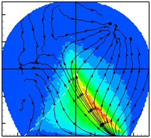
$q$– $r$ evolution strongly depends on the local streamline topology. The forcing action has a repeller at the bottom right corner of the plane, where local streamlines experience axisymmetric expansion. Forcing trajectories exhibit an attractor at the top right corner, that is, the rotation-dominated UFC topology, whereas some trajectories bend toward the left boundary of the plane (SFS topology). The effect of forcing is very weak in the rotation-dominated streamlines, whereas it is the strongest in the UN/S/S streamlines near the right zero-discriminant line. Comparing these trajectories with that of nonlinear, pressure and viscous action (figures 3, 4 and 5), it is clear that the repeller of forcing action nearly coincides with the attractors of nonlinear and viscous actions. This indicates that the key role of forcing is to counter the restricted Euler effect (Bikkani & Girimaji Reference Bikkani and Girimaji2007) in the region of Vieillefosse tail. Further, the forcing attractor in UFC region is close to the repeller of pressure action. Evidently, large-scale forcing strongly opposes nonlinear and viscous action in the strain-dominated streamline shapes, whereas it balances anisotropic pressure action in the rotation-dominated unstable focal streamline shapes.

Figure 8. The  $q$–
$q$– $r$ probability current due to forcing ( $\boldsymbol {W}_{F}$), with background contours representing the magnitude $|\boldsymbol {W}_F|$ for FIT ${Re_{\lambda }}=427$.
The relative magnitude of the forcing contribution with respect to the aggregate of nonlinear, pressure and viscous action is plotted as a percentage in figure 9. The contribution of forcing is comparable to that of nonlinear–pressure–viscous contribution in the nodal/hyperbolic streamlines, that is, below the discriminant line. The effect of forcing is weaker ( ${<}20\,\%$) in the focal/spiralling streamlines, that is, above the discriminant lines, except in the extremely high-density region. Overall, large-scale forcing plays a critical role toward sustaining the classical tear drop shape of the $q$–
$q$– $r$ joint p.d.f.

Figure 9. Relative contribution of forcing probability current with respect to the aggregate of nonlinear–pressure–viscous processes, that is,  $|\boldsymbol {W}_F|/(|\boldsymbol {W}_F| + |\boldsymbol {W}_{NPV}|) \times 100$, for FIT ${Re_{\lambda }}=427$. Contour levels are in an approximate log scale.
4.3. Helmholtz–Hodge decomposition of the probability currents
From (2.20), in a homogeneous statistically stationary turbulent flow, the stationarity of the  $q$–
$q$– $r$ p.d.f. requires that
 \begin{equation} \boldsymbol{\nabla}\boldsymbol{\cdot}\boldsymbol{W} = 0. \end{equation}
In order to maintain the statistical stationarity of the p.d.f., the principal role of forcing is to render the total probability flux vector  $\boldsymbol {W}$ dilatation free. Thus, more insight into the role of forcing and other processes on small-scale turbulence dynamics can be obtained by decomposing the probability current vectors in $q$–
$q$– $r$ phase space into dilatational and solenoidal parts:
 \begin{equation} \boldsymbol{W} = \boldsymbol{W}^{(dil)} + \boldsymbol{W}^{(sol)}. \end{equation}
The curl-free dilatational part and the divergence-free solenoidal part can be obtained by using the Helmholtz–Hodge decomposition of a two-dimensional vector field (Chorin & Marsden Reference Chorin and Marsden1979; Petronetto et al. Reference Petronetto, Paiva, Lage, Tavares, Lopes and Lewiner2009),
 \begin{equation} \boldsymbol{W}^{(dil)} = \boldsymbol{\nabla} \phi \quad \text{and} \quad \boldsymbol{W}^{(sol)} = J(\boldsymbol{\nabla} \psi), \end{equation}
where  $\phi$ and $\psi$ are scalar potential fields and $J(.)$ represents clockwise rotation of a vector by $90^{\circ }$. Here, the rotation operator applied to the gradient of scalar potential $\psi$ is analogous to the curl of a vector potential for a three-dimensional field. In general, there is also a harmonic term which has both zero divergence and zero curl, but that term is zero in this case due to boundary condition.
Segregating the effect of forcing from the other processes, equation (4.3) becomes
 \begin{equation} \boldsymbol{\nabla}\boldsymbol{\cdot} (\boldsymbol{W}_{NPV} + \boldsymbol{W}_F) = 0 \ \implies \ \boldsymbol{\nabla}\boldsymbol{\cdot} \boldsymbol{W}_{F} ={-} \boldsymbol{\nabla}\boldsymbol{\cdot} \boldsymbol{W}_{NPV}. \end{equation}
Helmholtz–Hodge decomposition of the forcing probability current as well as the nonlinear–pressure–viscous probability current results in
 \begin{gather} \boldsymbol{W}_F = \boldsymbol{W}^{(dil)}_F + \boldsymbol{W}^{(sol)}_F, \quad \text{where} \ \boldsymbol{W}_F^{(dil)} = \boldsymbol{\nabla} \phi_F \quad \text{and} \quad \boldsymbol{W}_F^{(sol)} = J(\boldsymbol{\nabla} \psi_F) ; \end{gather}
 \begin{gather} \boldsymbol{W}_{NPV} = \boldsymbol{W}^{(dil)}_{NPV} + \boldsymbol{W}^{(sol)}_{NPV} ,\quad \text{where} \boldsymbol{W}_{NPV}^{(dil)} = \boldsymbol{\nabla} \phi_{NPV} \quad \text{and} \quad \boldsymbol{W}_{NPV}^{(sol)} = J(\boldsymbol{\nabla} \psi_{NPV}). \end{gather}
The divergence of the solenoidal vector fields is zero by construction. Therefore, the condition (4.6) for a stationary process is
 \begin{equation} \boldsymbol{\nabla}\boldsymbol{\cdot} \boldsymbol{W}^{(dil)}_F ={-} \boldsymbol{\nabla} \boldsymbol{\cdot} \boldsymbol{W}^{(dil)}_{NPV} . \end{equation}
We now examine the DNS data to further analyse the role of dilatational and solenoidal components of the probability currents.
4.3.1. Dilatational and solenoidal current from DNS data
From (4.7a) the following can be obtained (Petronetto et al. Reference Petronetto, Paiva, Lage, Tavares, Lopes and Lewiner2009):
 \begin{equation} \boldsymbol{\nabla}\boldsymbol{\cdot} \boldsymbol{W}_F = \boldsymbol{\nabla}\boldsymbol{\cdot} \boldsymbol{W}_F^{(dil)} = \Delta \phi_F {,}\quad \boldsymbol{\nabla} \times \boldsymbol{W}_F = \boldsymbol{\nabla} \times \boldsymbol{W}_F^{(sol)} ={-} \Delta \psi_F , \end{equation}
where  $\Delta$ is the Laplacian operator ( $\Delta \equiv \nabla ^{2}$). The system of Poisson equations (4.9a,b) is numerically solved in the bounded $q$–
$q$– $r$ domain ( $\varOmega$) to determine the potential functions $\phi _F(q,r)$ and $\psi _F(q,r)$. The solenoidal vector field is taken to be tangential at the boundary of the domain ( $\partial \varOmega$). The boundary condition for the dilatational vector field is chosen such that it is compatible with that of the total vector field at the boundary. The resulting system of Poisson equations and boundary conditions is given by
 $$\begin{gather} \Delta \phi_F = \boldsymbol{\nabla}\boldsymbol{\cdot} \boldsymbol{W}_F \quad \text{and}\quad \Delta \psi_F ={-} \boldsymbol{\nabla} \times \boldsymbol{W}_F \quad \text{in} \ \varOmega , \end{gather}$$
 $$\begin{gather}\boldsymbol{\nabla} \phi_F\boldsymbol{\cdot} \hat{\boldsymbol{n}} = \boldsymbol{W}_F \boldsymbol{\cdot} \hat{\boldsymbol{n}} \quad \text{and}\quad J(\boldsymbol{\nabla} \psi_F) \boldsymbol{\cdot} \hat{\boldsymbol{n}} = 0 \quad \text{in} \ \partial \varOmega . \end{gather}$$
Here,  $\hat {\boldsymbol {n}}$ represents the outward normal vector at the boundary of the domain. The rectangular $q$–
$q$– $r$ domain is discretised into $100\times 100$ points and second-order accurate central difference scheme is used to solve the above system of equations. A convergence study is performed to ensure that the solution does not change with increasing $q$–
$q$– $r$ space resolution. While solving the discrete system of equations with pure Neumann boundary conditions, the issue of non-uniqueness of the solution is encountered. An augmented system of equations (Rosales et al. Reference Rosales, Seibold, Shirokoff and Zhou2020) is solved with an additional scalar variable (Lagrange multiplier) to impose a restriction on the sum of the scalar potential. This, in turn, satisfies the discrete compatibility condition and enforces uniqueness of the solution up to an additive constant (Barton & Barton Reference Barton and Barton1989; Rosales et al. Reference Rosales, Seibold, Shirokoff and Zhou2020). Once the scalar potentials, $\phi _F(q,r)$ and $\psi _F(q,r)$, are obtained for the entire $q$–
$q$– $r$ plane, the dilatational and solenoidal vector components of $\boldsymbol {W}_F$ are determined from their gradients (see (4.7a)). A similar procedure is followed to compute the dilatational and solenoidal components of $\boldsymbol {W}_{NPV}$, as given in (4.7b).
The dilatational parts of  $\boldsymbol {W}_F$ and $\boldsymbol {W}_{NPV}$ are plotted in figures 10(a) and 10(b), respectively. The background colour contours represent the local speed of the trajectories. The $\boldsymbol {W}^{(dil)}_F$ probability current has an attractor at the bottom right corner of the plane (axisymmetric expansion) and a repeller in the rotation-dominated unstable focal streamlines. In contrast, the dilatational part of the nonlinear–pressure–viscous contribution ( $\boldsymbol {W}^{(dil)}_{NPV}$), has a repeller in the rotation-dominated UFC topology and an attractor near the axisymmetric expansion. Thus, the repeller of one nearly coincides with the attractor of the other and vice versa. In addition, the magnitudes of the probability currents at different $q$–
$q$– $r$ locations are similar in both cases. The magnitudes reduce in value as $q$ becomes more positive, that is, rotation-dominated. The dilatational part of the forcing action is approximately negative of the dilatational part of the nonlinear–pressure–viscous action. Although there are minor differences between the two fields, the sum of the divergence of $\boldsymbol {W}^{(dil)}_F$ and $\boldsymbol {W}^{(dil)}_{NPV}$ is nearly zero throughout the domain, as required for statistical stationarity (4.8).

Figure 10. Dilatational parts of (a) forcing probability current  $\boldsymbol {W}^{(dil)}_{F}$ and (b) nonlinear–pressure–viscous probability current $\boldsymbol {W}^{(dil)}_{NPV}$, for FIT ${Re_{\lambda }}=427$. The background contours represent the magnitude of the vector.
In figure 11, the dilatational parts of the nonlinear–pressure–viscous currents are plotted for FIT and turbulent channel flow at different Reynolds numbers. It is evident that the dilatational  $\boldsymbol {W}_{NPV}$ currents are qualitatively similar in both types of flows. There are minor differences in the magnitude of the probability current, which can likely be attributed to the difference in ${Re_{\lambda }}$ and inhomogeneity of the channel flow case in the wall-normal direction as discussed in § 4.1.

Figure 11. Dilatational parts of nonlinear–pressure–viscous probability current  $\boldsymbol {W}^{(dil)}_{NPV}$ for (a) FIT ${Re_{\lambda }}=225$, (b) FIT ${Re_{\lambda }}=385$ and (c) channel flow ${Re_{\lambda }}=132$. The background contours represent the magnitude of the vector.
The solenoidal parts of  $\boldsymbol {W}_F$ and $\boldsymbol {W}_{NPV}$ are plotted in figures 12(a) and 12(b), respectively. It is first evident that the solenoidal component of forcing is smaller in magnitude than its dilatational counterpart (figure 10a), over most of the $q$–
$q$– $r$ plane. On the other hand, the magnitude of the solenoidal part of $\boldsymbol {W}_{NPV}$ is much larger than its dilatational part (figure 10b) in most of the $q$–
$q$– $r$ plane. Now, the solenoidal components are divergence free by construction and form closed-loop trajectories in the $q$–
$q$– $r$ plane. The solenoidal forcing, $\boldsymbol {W}_F^{(sol)}$, exhibits two centres in the domain about which the trajectories orbit. One centre lies on the left zero-discriminant line and the other is in the UFC topology slightly above the right zero-discriminant line. The solenoidal part of nonlinear–pressure–viscous effects, $\boldsymbol {W}^{(sol)}_{NPV}$, is significantly higher in magnitude than $\boldsymbol {W}_F^{(sol)}$. It consists of closed periodic orbits around a centre located near the origin. The closed-loop trajectories appear to slow down substantially in the nodal/hyperbolic topology region in the plane. There exists another centre near the right boundary of the $q$–
$q$– $r$ plane, in the extremely low-density region. It is important to note that the solenoidal $NPV$ probability current is very similar to the total probability current in figure 7, especially in the sufficiently populated regions of the plane.

Figure 12. Solenoidal parts of: (a) forcing probability current  $\boldsymbol {W}^{(sol)}_{F}$ and (b) nonlinear–pressure–viscous probability current $\boldsymbol {W}^{(sol)}_{NPV}$, for FIT ${Re_{\lambda }}=427$. The background contours represent the magnitude of the vector.
The key findings from this analysis can be summarised as follows.
(i) The most important role of large-scale forcing is to oppose and nullify the dilatational probability current due to inertial, pressure and viscous effects.
(ii) The solenoidal part of forcing current is considerably smaller in magnitude and, hence, plays a secondary role in VG dynamics.
(iii) The solenoidal part of nonlinear–pressure–viscous probability current dominates the overall dynamics of VG tensor invariants. For the most part,
$\boldsymbol {W}^{(sol)}_{NPV}$ dictates the universal features of the small-scale dynamics.

In summary, in order to maintain a statistically stationary p.d.f. (2.20), the dilatational part of nonlinear–pressure–viscous probability current must be neutralised by the dilatational part of forcing current. Thus, the magnitude of forcing must be large enough to affect this balance, as has been demonstrated in this section. The observable effect of forcing on VG dynamics comes only from the solenoidal part of forcing probability currents, which is shown to be significantly smaller than that of the other three. Thus, the solenoidal nonlinear–pressure–viscous probability current is responsible for most of the observable VG dynamics.
5. VG magnitude dynamics
The p.d.f. of the standardised variable
 \begin{equation} \theta^{*}= \frac{\theta - \langle \theta \rangle}{\sigma_\theta} \quad \text{where} \ \theta \equiv \ln{A} ,\quad \sigma_\theta = \sqrt{ \langle (\theta - \langle \theta \rangle)^{2} \rangle } \end{equation}
is displayed in figure 13(a) for FIT at  ${Re_{\lambda }}=225$, $385$ and $427$ and channel flow at ${Re_{\lambda }}=81$, $110$ and $132$. The p.d.f. of standard normal distribution, with zero mean and unit standard deviation, is also plotted in the figure for comparison. Clearly, the p.d.f.s of $\theta ^{*}$ for both FIT and channel flow at all ${Re_{\lambda }}$ nearly coincide with that of the normal distribution (Obukhov Reference Obukhov1962; Yeung & Pope Reference Yeung and Pope1989). It must be noted, however, that due to intermittency, the p.d.f. of pseudo-dissipation cannot be precisely log-normal (Orszag Reference Orszag1970; Mandelbrot Reference Mandelbrot1999). To illustrate this further, the p.d.f.s are plotted in the log–linear scale in figure 13(b), which shows some dependence on ${Re_{\lambda }}$ and the type of forcing in the flow. However, the overall probability distribution of VG magnitude is close to (but not precisely) log-normal in turbulent flows of different Reynolds numbers. We now investigate the role of different turbulence processes in the dynamics of the VG magnitude of statistically stationary turbulence.

Figure 13. P.d.f. of  $\theta ^{*}$ for FIT at ${Re_{\lambda }}=225$, $385$ and $427$ (dashed or dash-dotted lines), for channel flow at ${Re_{\lambda }}=81$, 110, 132 (solid lines with symbols) and for a standard normal distribution (solid line) in (a) linear–linear scale and (b) log–linear scale.
5.1. VG magnitude dynamics conditioned on $q$–$r$


The total rate of change of  $\theta$ is calculated by following the same procedure and guidelines used for $q$ and $r$ in § 4.2. The rate of change of $\theta$ due to the different processes (2.22a,b) is conditioned on $q$–
$q$– $r$ and plotted in figure 14. The nonlinear ( $N$) action is predominantly positive in the high-density regions of the $q$–
$q$– $r$ plane, particularly along the right discriminant line including the axisymmetric expansion. Thus, nonlinear contribution increases the VG magnitude in most of the turbulent flow field. Nonlinear action diminishes the VG magnitude along the left discriminant line, especially at axisymmetric compression. Pressure ( $P$) opposes the nonlinear effect in the strain-dominated topologies ( $q<0$) with the exception of the UFC region. It, however, augments the nonlinear action in the rotation-dominated topologies ( $q>0$). This behaviour is unlike the $q$–
$q$– $r$ probability current, where pressure opposes nonlinear action in both strain- and rotation-dominated topologies alike. The viscous ( $V$) action shows a relatively weaker dependence on the local streamline topology and is negative throughout the $q$–
$q$– $r$ plane. In other words, viscosity tries to diminish the VG magnitude at all streamline topologies. It is important to note that the viscous action opposes the nonlinear action in the densely populated regions of the plane.

Figure 14. Conditional mean rate-of-change of  $\theta$ ( ${\equiv }\ln A$) in $q$–
$q$– $r$ phase plane due to: (a) nonlinear, (b) pressure, (c) viscous, (d) nonlinear–pressure–viscous, (e) forcing and (f ) all processes for FIT ${Re_{\lambda }}=427$.
The aggregate of nonlinear, pressure and viscous ( $NPV$) processes in each of the four quadrants of the $q$–
$q$– $r$ plane can be summarised as follows: it increases VG magnitude in rotation-dominated stable and strain-dominated unstable topologies; it decreases VG magnitude in rotation-dominated unstable and strain-dominated stable topologies. It is the strongest in the rotation-dominated unstable (UFC) topology.
Expectedly, the forcing ( $F$) contributes toward increasing VG magnitude nearly uniformly at all $q$–
$q$– $r$ values. The conditional mean effect of forcing in the $q$–
$q$– $r$ plane is weaker than the other processes. Although the viscous and forcing effects are nearly independent of topology, the nonlinear and pressure effects on the evolution of VG magnitude are strongly dependent on $q$–
$q$– $r$. As a result, the net rate of change of VG magnitude due to the combination of all four processes (figure 14f) is a strong function of topology. On average, the VG magnitude increases in the SFS, UN/S/S and strain-dominated UFC topologies, and it decreases in the SN/S/S and rotation-dominated UFC topologies. It is further evident that this resulting total evolution of VG magnitude is primarily driven by the aggregate of nonlinear–pressure–viscous action with a small but distinct influence of large-scale forcing.
5.2. VG magnitude dynamics conditioned on $\theta ^{*}$

The conditional mean rate-of-change of  $\theta$ (2.24)–(2.25) is plotted as a function of the standardised variable $\theta ^{*}$ in figure 15(a). The total conditional mean rate of change ( $\tilde {u}$) is nearly equal to zero at all $\theta ^{*}$. This satisfies the statistical stationarity condition given in (2.26). The nonlinear ( $N$) term is positive at all magnitudes, whereas the viscous ( $V$) effect is always negative. The pressure ( $P$) and forcing ( $F$) action exhibit different behaviours in different ranges of $\theta$.

Figure 15. Conditional mean rate-of-change of  $\theta$ ( ${\equiv }\ln A$) conditioned on $\theta ^{*}$ due to the processes: (a) nonlinear, pressure, viscous, forcing and total for FIT ${Re_{\lambda }}=427$ case and (b) nonlinear (red), pressure (blue) and viscous (green) for FIT ${Re_{\lambda }}=86,225,427$ (dashed lines) and channel flow ${Re_{\lambda }}=81,110,132$ (solid lines).
The positive nonlinear effect on the rate of change of VG magnitude grows rapidly as the VG magnitude increases. On the other hand, the viscous action becomes increasingly negative with VG magnitude, balancing the nonlinear contribution. At extremely low VG magnitudes ( $\theta \leqslant \langle \theta \rangle - 2 \sigma _\theta$), the nonlinear effects are weak, whereas the positive pressure and forcing contributions are balanced by a negative viscous action. At moderately small VG magnitudes ( $\langle \theta \rangle -2\sigma _\theta \leqslant \theta \leqslant \langle \theta \rangle$), the nonlinear and viscous contributions begin to grow rapidly with $\theta ^{*}$. In this range, positive pressure and forcing contributions add to the increasingly positive nonlinear action, and their aggregate is balanced by a strongly negative viscous action. At intermediate VG magnitudes ( $\langle \theta \rangle \leqslant \theta \leqslant \langle \theta \rangle + 2\sigma _\theta$), the pressure action becomes negative, while forcing contribution remains positive. The behaviour of pressure and forcing switch as VG magnitude reaches a higher value ( $\theta \geqslant \langle \theta \rangle + 2 \sigma _\theta$). At high VG magnitudes, forcing action becomes increasingly negative to balance the equally positive pressure action. Thus, in regions of very high VG magnitudes, forcing makes a surprising negative contribution toward $\theta$ evolution.
The dynamical behaviour of VG magnitude is similar in isotropic turbulence and turbulent channel flow at different Taylor Reynolds numbers, as shown in figure 15(b), for the nonlinear, pressure and viscous processes. Some differences are observed at high  $\theta ^{*}$ ( $>2$), which is consistent with the variations in the p.d.f. tails of $\theta ^{*}$ (figure 13b) in this range.
The key findings are: (i) the total conditional mean rate of change of VG magnitude is nearly zero at all magnitudes; (ii) at high VG magnitudes, there is a clear balance between pressure and forcing on the one hand and viscous–inertial balance on the other; and (iii) at smaller VG magnitudes the viscous action balances all the other processes.
The insight and observations highlighted in this work provide important guidance for modelling VG dynamics. Numerous studies in literature have presented Langevin VG models to capture the Lagrangian evolution of VG tensor in turbulent flows (Girimaji & Pope Reference Girimaji and Pope1990; Jeong & Girimaji Reference Jeong and Girimaji2003; Chevillard & Meneveau Reference Chevillard and Meneveau2006; Johnson & Meneveau Reference Johnson and Meneveau2016). Most of these studies have focused on developing closure models to capture the non-local pressure and viscous effects on VG dynamics. We propose that inclusion of the ‘universal’ forcing effects, presented in this work, will lead toward improved VG modelling in turbulent flows.
6. Unnormalised VG invariants dynamics
The unnormalised VG invariants ( $Q,R$), commonly used for topological classification of local streamline shape in turbulent flows (Chong et al. Reference Chong, Perry and Cantwell1990), is a combination of the streamline shape ( $q,r$) and scale ( $A$). Although it defines topology, it does not uniquely determine the geometric shape of the streamlines and its dynamics is unable to capture some of the key effects of different turbulence processes on VGs (Das & Girimaji Reference Das and Girimaji2020). The CMTs in the $Q$–
$Q$– $R$ plane due to pressure, viscous and nonlinear effects have been studied extensively in the past (Martín et al. Reference Martín, Ooi, Chong and Soria1998; Ooi et al. Reference Ooi, Martin, Soria and Chong1999; Chevillard et al. Reference Chevillard, Meneveau, Biferale and Toschi2008; Johnson & Meneveau Reference Johnson and Meneveau2016). Thus, for the sake of completeness and further insight, in this section we illustrate the effect of forcing in the unnormalised $Q$–
$Q$– $R$ plane.
The probability current,  $\boldsymbol {\tilde {W}}$, of $Q^{*}$– $R^{*}$, where $Q^{*}=Q/\langle A_{ij} A_{ij} \rangle$ and $R^{*}=R/\langle A_{ij} A_{ij} \rangle ^{3/2}$, is given by
 \begin{equation} \boldsymbol{\tilde{W}} = \tilde{\mathcal{F}}(Q^{*},R^{*}) \times \left \langle\left. \begin{pmatrix} {\rm d}Q^{*}/{\rm d}t\\ {\rm d}R^{*}/{\rm d}t \end{pmatrix} \right | Q^{*},R^{*} \right \rangle, \end{equation}
where  $\tilde {\mathcal {F}}(Q^{*},R^{*})$ is the $Q^{*}$– $R^{*}$ joint p.d.f. The $Q^{*}$– $R^{*}$ probability currents due to nonlinear, pressure, viscous and forcing processes as well as the total probability currents, computed following the same procedure as outlined in §§ 4.1 and 4.2 for $q$–
$q$– $r$, are plotted in figure 16 for the FIT case of $Re_\lambda =427$. The probability currents due to the inertial, pressure and viscous effects resemble the CMTs illustrated in the previous studies (Martín et al. Reference Martín, Ooi, Chong and Soria1998; Chevillard et al. Reference Chevillard, Meneveau, Biferale and Toschi2008; Johnson & Meneveau Reference Johnson and Meneveau2016; Das & Girimaji Reference Das and Girimaji2020). The total probability current trajectories form nearly closed loops with small errors arising from the numerical computation of material derivatives of $Q^{*}$ and $R^{*}$. The nearly closed-loop trajectories indicate the stationarity of the $Q^{*}$– $R^{*}$ joint p.d.f. The probability currents due to the nonlinear (inertial and isotropic pressure) effects take trajectories from left to the right following the zero-discriminant line similar to the $q$–
$q$– $r$ trajectories in figure 3. The anisotropic pressure probability currents primarily oppose the nonlinear action taking trajectories from the right to the left as in the $q$–
$q$– $r$ plane (figure 4). The viscous probability currents are dominated by the damping effect of viscosity on VG magnitude and as a result all the trajectories simply collapse to the origin. As previously pointed out in Das & Girimaji (Reference Das and Girimaji2020), the finer details of viscous action on local streamline geometric shape as observed in the $q$–
$q$– $r$ plane (figure 5) are not visible in the $Q^{*}$– $R^{*}$ plane. The probability currents due to forcing in the $Q^{*}$– $R^{*}$ plane (figure 16e) clearly illustrate some of the key features observed in the $q$–
$q$– $r$ plane (figure 8). The repellers of this system (the right discriminant line and the origin) coincide with the attractors of the nonlinear and viscous effects (figures 16b and 16d) which indicates that forcing opposes inertial and viscous action, similar to the $q$–
$q$– $r$ plane. Trajectories are attracted toward the top right unstable focal topology region and toward the left bottom strain-dominated part of the plane, displaying further similarities with the $q$–
$q$– $r$ forcing currents. In the $q$–
$q$– $r$ plane, forcing opposes anisotropic pressure effects in the unstable rotation-dominated streamline shapes. This effect of forcing is obscured in the $Q^{*}$– $R^{*}$ plane due to the presence of the magnitude dynamics, in which forcing supports anisotropic pressure action (figure 15) at lower VG magnitudes.

Figure 16. The  $Q^{*}$– $R^{*}$ probability currents ( $\boldsymbol {\tilde {W}}$) due to (a) total, (b) nonlinear, (c) anisotropic pressure, (d) viscous and (e) forcing effects, for FIT at ${Re_{\lambda }}=427$. The VG invariants are normalised as $Q^{*}=Q/\langle A_{ij}A_{ij} \rangle$, $R^{*}=R/\langle A_{ij}A_{ij} \rangle ^{3/2}$. The background contours represent the magnitude of the probability current vector $\boldsymbol {\tilde {W}}(Q^{*},R^{*})$. The white dashed lines are the zero discriminant lines.
7. Conclusions
It is generally accepted that at high enough Reynolds numbers, the small scales of turbulence behave in a manner that is universal and insensitive to the large-scale features of turbulence. However, the large and small scales are coupled by the cascade process. Indeed, without large-scale forcing and the subsequent cascade, turbulence cannot be sustained at the small scale. The overall implication is that the effect of large-scale forcing on the small scales is similar across different flow types. In this work, we identify the precise role of large-scale forcing on the ‘universal’ small-scale VG dynamics using DNS data of simple canonical flows. To demarcate and isolate the effects of intermittency, the effect of forcing on the VG magnitude ( $A \equiv \sqrt {A_{ij}A_{ij}}$) and the normalised VG tensor ( $b_{ij} \equiv A_{ij}/A$) are examined independently.
First, the evolution equations of  $b_{ij}$-invariants ( $q,r$) and VG magnitude $A$ are derived, along with their p.d.f. equations. DNS data sets of FIT and turbulent channel flow are used to investigate the $q$–
$q$– $r$ joint p.d.f. and the underlying probability currents due to various turbulence processes. It is first shown that the characteristic tear-drop-shaped $q$–
$q$– $r$ joint p.d.f. asymptotes toward a self-similar form at high enough Reynolds numbers. The $q$–
$q$– $r$ joint p.d.f.s for isotropic turbulence and turbulent channel flow are shown to be nearly identical. The probability currents due to inertial, pressure and viscous effects are also very similar in both flows.
The combined probability currents of inertial, pressure and viscous effects is not closed loop and cannot sustain the stationary tear-drop p.d.f. shape. This clearly indicates that forcing plays a pivotal role in forming and sustaining the tear-drop  $q$–
$q$– $r$ joint p.d.f. shape. Next, the flow-independent effect of large-scale forcing on $q$–
$q$– $r$ evolution is examined using FIT data. The effect of forcing is shown to be strongly dependent on the local topology. Forcing effects on local streamline shape are much stronger in locally nodal/hyperbolic streamlines than in focal/spiralling streamlines. The forcing action strongly opposes the inertial and viscous action in these nodal streamlines, whereas it counters the anisotropic pressure action in the unstable focal streamlines. It is further shown that the dilatational part of the forcing probability current balances the dilatational part of the inertial–pressure–viscous contribution at all topologies. The solenoidal part of forcing current is relatively smaller than that of the inertial–pressure–viscous effects. To a leading order, the solenoidal part of inertial–pressure–viscous action dictates the overall evolution of trajectories in the $q$–
$q$– $r$ phase space.
The effect of large-scale forcing along with the inertial, pressure and viscous processes on the evolution of VG magnitude is examined by conditioning these processes on the invariants phase space and on the VG magnitude itself. At smaller magnitudes, forcing along with inertia and pressure opposes the strongly negative viscous action. At larger magnitudes, forcing balances the increasingly positive pressure action, whereas viscosity counteracts the inertial action. The forcing contribution to the mean rate of change of VG magnitude is nearly independent of topology ( $q,r$). The nonlinear–pressure–viscous action drives the overall conditional mean evolution of VG magnitude in the $q$–
$q$– $r$ plane, with a weaker but discernible influence of forcing. Altogether, the rotation-dominated unstable focal topology and the stable nodal topology exhibit overall diminishing VG magnitude, whereas all the other topologies demonstrate overall growing VG magnitude. In the unnormalised invariants ( $Q$–
$Q$– $R$) plane, the effect of forcing illustrates only some of the dynamics that are observed in the streamline shape ( $q$–
$q$– $r$ plane) and VG magnitude individually. Overall, these findings further our understanding of VG dynamics and suggest important simplifications that can be used for the development of improved VG models.
Declaration of interests
The authors report no conflict of interest.


 Open access