


1 Introduction
Most combustion systems are designed to operate in stable regimes but it is known that, ‘sometimes’, combustion systems exhibit unwanted oscillations. These combustion instabilities, also designated as thermoacoustic instabilities, are a manifestation of combustion dynamics. They can lead to high amplitude noise and vibration levels. In the worst cases, the resulting oscillations of the flow may give rise to flashback, a process in which the flame moves into the injector units and reaches the upstream manifold with serious consequences to the system integrity. In some cases, the large amplitude oscillations induce flame quenching or partial or total blow-off. The pressure oscillations can also become large enough to damage the combustor structure or lead to the destruction of the system.
Due to their detrimental consequences in engines, power and heat generation units, combustion instabilities (CIs) are an important field of combustion research, combining the various disciplines involved in reacting flows (fluid mechanics, thermodynamics, kinetics and transport) but also requiring the introduction of acoustics, hydrodynamic stability, system dynamics and control theory. The progress made since the initial developments in the 1950s in predicting, controlling and damping these undesirable self-sustained combustion oscillations can be gauged in the successive reviews from Crocco & Cheng (Reference Crocco and Cheng1956), Putnam (Reference Putnam1971), McManus, Poinsot & Candel (Reference McManus, Poinsot and Candel1993), Candel (Reference Candel2002), Dowling & Morgans (Reference Dowling and Morgans2005), Lieuwen & Yang (Reference Lieuwen and Yang2005), Culick (Reference Culick2006), Huang & Yang (Reference Huang and Yang2009), Gicquel, Staffelbach & Poinsot (Reference Gicquel, Staffelbach and Poinsot2012), O’Connor, Acharya & Lieuwen (Reference O’Connor, Acharya and Lieuwen2015), Poinsot (Reference Poinsot2017) and Juniper & Sujith (Reference Juniper and Sujith2018) and in the books from Poinsot & Veynante (Reference Poinsot and Veynante2012) and Lieuwen (Reference Lieuwen2012).
One of the striking features in these references is that combustion instabilities may arise in a wide variety of combustion systems. This includes, at one end, devices operating with unconfined flames powered by a gaseous fuel with less than one kilowatt thermal power output and, at the other end, rocket engines in which the combustion of liquid or solid propellants at high pressure delivers several gigawatts of thermal power. These instabilities can either be coupled by axial or transverse acoustic modes of the system, as in annular gas turbines, and their frequencies may span from a few Hertz, as observed in large industrial boilers featuring a bulk flow oscillation through the entire boiler, up to several kilo Hertz when coupled to a transverse mode as in the small thrust chamber of liquid rocket engines.
While the ultimate objective is to predict and control CIs in real large-scale turbulent combustors, understanding combustion instabilities in laminar systems is obviously a necessary first step. Many practical systems also operate in a premixed laminar mode and often suffer from CIs. Over the last 50 years, the analysis of the dynamics of laminar premixed systems has proved to be surprisingly difficult, leading to a large research effort, see for example Ducruix et al. (Reference Ducruix, Schuller, Durox and Candel2003) and De Goey et al. (Reference De Goey, van Oijen, Kornilov and ten Thije Boonkkamp2011). Many of the analytical developments made in Lieuwen (Reference Lieuwen2012) are for laminar systems. It is also worth noting that a new class of intrinsic thermoacoustic instabilities has been recently highlighted with the help of laminar combustion experiments (Hoeijmakers et al. Reference Hoeijmakers, Kornilov, Arteaga, de Goey and Nijmeijer2014; Emmert et al. Reference Emmert, Bomberg, Jaensch and Polifke2015).
Premixed laminar flames have an interesting specificity. Because of the simplicity of the base flow, they can be studied using experiments, pure theory or direct numerical simulation (DNS). They are probably the most complicated canonical flames for which all three approaches can be used simultaneously. The capacity of combining these three approaches and the clean flow conditions in which these flames can be studied, make laminar premixed flames ideal configurations for investigating flame dynamics. Results obtained on these flames may then serve as a guide for more complex cases.

Figure 1. (a) Feedback loop of thermoacoustic instabilities and (b) open loop flame transfer function  $\text{FTF}=G(\unicode[STIX]{x1D714}_{r})\exp (\text{i}\unicode[STIX]{x1D711}(\unicode[STIX]{x1D714}_{r}))$.
The objectives of this article are to provide an overview of the knowledge in combustion dynamics, starting from basic descriptions of acoustically coupled combustion instabilities in laminar premixed systems and closing with some recent research results. The paper is focused on premixed and laminar flames but many results apply to other types of flames as well. It is organized to provide a theoretical framework allowing analysis of CIs coupled by longitudinal as well as azimuthal acoustic modes.
The goal is to focus on analytical results obtained with the help of a series of simplifications to highlight the critical roles of the injector and flame responses to flow perturbations in the development of instabilities. Analytical expressions for the conditions leading to instabilities are derived for a set of generic configurations featuring the main components of real combustors. These results are used to discuss the respective influence of the injector dynamics and flame response. Finally, a theoretical framework is derived to model the flame response to flow-rate and mixture composition disturbances. It is illustrated in a simple case how the flame response can be tailored to reduce its susceptibility to flow perturbations.
Before examining the way acoustic waves interact with the flow and flame dynamics, it is worth describing the feedback loop leading to combustion instability. Thermoacoustic instabilities in combustion systems are due to synchronized oscillations between heat release rate disturbances produced by the flame and acoustic perturbations as illustrated in figure 1(a). In the absence of unsteady heat release, this coupling ceases. The main assumption which is used in this work, as in many others, is that the flame response to incoming flow perturbations produced by an external actuator in a stable configuration of the combustor can be used to assess the combustor dynamic stability, i.e. its capacity to induce self-sustained combustion oscillations without external actuator (Candel Reference Candel2002). In the diagram in figure 1, this means that the flame response characterized in terms of heat release rate oscillations can be studied outside the acoustic feedback loop shown in figure 1(a) by submitting the flame to acoustic disturbances to get the gain and phase information displayed in figure 1(b). This ‘open loop’ analysis leads to the definition of a flame transfer function (FTF) linking heat release rate disturbances to acoustic modulations produced by externally forcing the flow, as will be defined more precisely in § 2.
Another remarkable feature of combustion instabilities is that acoustic laws remain generally valid for the perturbed flow except at very high sound levels. Assuming acoustic disturbances and vanishingly small heat release rate perturbations, the FTF combined with an acoustic model of the combustor provides a framework for the linear stability analysis of the system dynamics. The gain  $G$ and phase lag $\unicode[STIX]{x1D711}$ of the FTF (see figure 1b) can be determined from experiments, simulations or theory. The frequencies $f=\unicode[STIX]{x1D714}_{r}/2\unicode[STIX]{x03C0}$ and the growth rates $\unicode[STIX]{x1D714}_{i}$ of the unstable modes are deduced by examining the stability of the closed-loop system in figure 1(a). Decoupling the acoustic analysis of the combustor from the analysis of the flame response to external flow disturbances has been so successful over the past two decades that it is now used by industry during the design process of real combustors (Lieuwen & Yang Reference Lieuwen and Yang2005). This framework underlies the theoretical analysis exploited in the present article.
When the oscillation level of the instability increases in the combustor, nonlinearity is first manifested in the flame response by saturation of the gain and eventually also by a shift of the phase lag compared to its response at a lower perturbation amplitude. This is due to the strong nonlinearity of the heat release rate. The other flow perturbations remain in this respect less altered by the oscillation level and can often be considered to remain in the linear acoustic regime. Recognizing this feature, Dowling (Reference Dowling1999) and Noiray et al. (Reference Noiray, Durox, Schuller and Candel2008) developed a weakly nonlinear framework in which the linear FTF filter is replaced by a nonlinear flame describing function (FDF) that accounts for effects of the perturbation level. The FDF corresponds to a set of FTFs, each determined for a range of forcing levels as illustrated in figure 2(a). Once the FTFs are determined, the methodology developed by Noiray et al. (Reference Noiray, Durox, Schuller and Candel2008) shows how to use the FDF to predict limit cycle oscillation levels and their corresponding frequencies.
The FDF framework is a natural extension of a linear stability analysis based on FTF, in which the mode frequencies and their growth rates are calculated repeatedly for increasing forcing levels for which the FDF is known. The stability diagram is finally deduced from an analysis of the growth rate trajectories as a function of the acoustic level in the combustor. An example is given in figure 2(b). This strategy has been shown to be quite successful in determining the oscillation level of combustion instabilities reaching a limit cycle in several combustors, including configurations with complex geometries and multiple burners.

Figure 2. (a) Typical evolution of the gain  $G$ and phase lag $\unicode[STIX]{x1D711}$ of a flame describing function (FDF) as the acoustic forcing level increases. (b) Growth rate $\unicode[STIX]{x1D714}_{i}$ of an unstable mode as a function of the acoustic forcing level leading to a limit cycle.
In this paper, the expressions derived for the frequencies and growth rates of instabilities are determined explicitly as a function of the gain  $G$ and phase lag $\unicode[STIX]{x1D711}$ of the FTF, meaning that the same expressions can be used to conduct a weakly nonlinear analysis provided that the FTF is replaced by the FDF in these expressions. An analysis of the growth rate trajectories such as the one in figure 2 can then be carried out without difficulty. This is why the rest of the paper focuses on linear acoustic perturbations and vanishingly small heat release rate disturbances, remembering that it is easy to extend the analysis by replacing the FTF by the FDF.
Basic principles of flame acoustic interactions are reviewed in § 2. Axial mode coupling is examined in § 3 for flames burning inside a combustion chamber and unconfined flames stabilized at the top of a burner. A system featuring a Helmholtz mode associated with a bulk flow oscillation is also examined. The existence and properties of intrinsic dynamical oscillations are discussed in § 4. Coupling involving azimuthal modes in annular combustion chambers is examined in § 5. The analysis takes into account a common plenum feeding a set of injectors and the impedance of these injectors. Results for the frequencies and growth rates of combustion instabilities derived in §§ 3 to 5 make use of the FTF, which is assumed to be known. The response of premixed flames to mixture and flow-rate perturbations is then revisited in § 6. This is used to show how the FTF may be obtained analytically, to highlight the role of the flame root dynamics and demonstrate how tailoring the FTF by passive or by active means can be used to lower heat release rate disturbances. References are provided in each of these sections as required by the developments. This is not intended to be an exhaustive review of the literature and many more references may be found in the cited articles.
2 Tutorial on thermoacoustics

Figure 3. Examples of tubes in which self-sustained pressure oscillations are driven by heat addition.
Thermoacoustic oscillations generally imply a driving process that is in most cases the heat released by combustion and a coupling mechanism that in most cases takes the form of resonant acoustic modes of the system. The most common thermoacoustic oscillations are driven by flames but there are examples where the oscillation is produced by another thermal process. A well-known configuration is that of the ‘Rijke’ tube that comprises a pipe and a heat source which may be a flame inserted in the tube, a metallic gauze that is initially preheated or an electrically heated resistive wire arrangement (Rijke Reference Rijke1859a,Reference Rijkeb; Mariappan & Sujith Reference Mariappan and Sujith2011). Raun et al. (Reference Raun, Beckstead, Finlinson and Brooks1993) list a series of devices made of tubes with heat addition leading to thermoacoustic instabilities, some of which are illustrated in figure 3. Sound is generated in these configurations at one of the resonant frequencies of the tube. This is perhaps the simplest device for demonstrations but may not be the best idealization of more practical situations.
The analysis of combustion instabilities requires a coupling of descriptions of the unsteady combustion process on one hand with the acoustics of the system on the other hand. There are many complexities in these two items, so that simplifications are usually needed to develop the analysis.
One-dimensional acoustics is often assumed because acoustic waves involved in many CIs are approximately planar, one-dimensional perturbations progressing in the axial direction. In this respect, the acoustics involved in CIs are simpler than that arising in aeroacoustic problems where propagation is essentially three-dimensional or takes the form of higher-order duct modes. It is worth noting, however, that combustion systems often feature a complex geometry and this may require multidimensional calculations based on a Helmholtz solver to determine the acoustic field in the system. Section 2.1 presents the basic elements governing acoustic wave propagation in one-dimensional systems. In cases where the wavelength is of the order of or smaller than a typical transverse dimension of the system, combustion may couple to transverse acoustic modes featuring a more complex two-dimensional distribution that is considered in § 5.
Acoustic impedance characteristics are of central importance in CI analysis. This quantity introduced in § 2.2 is used to describe the acoustic response of inlet(s) and outlet(s) of combustors. In many instances, these impedances essentially control the stability of the system because they determine how much acoustic energy is reflected into the chamber and define the phase of the reflected field with respect to the incident waves.
During CIs, flames are submitted to unsteady motion caused by the flow perturbations entering the flame zone. Over the years, one approach has proved to be sufficiently powerful to analyse CIs and simple enough to be implemented in most models in the form of a FTF. In this framework, the response of the flame stabilized over an injector in a flow at fixed equivalence ratio depends directly on one single quantity, the inlet velocity. This concept is presented in § 2.3. Section 6 shows how to model this function by taking into account flow rate, as well as mixture composition perturbations.
Stability analysis based on FTF is introduced in § 2.4. The method is important because it is not feasible to analyse combustion dynamics issues by only resorting to multidimensional simulations of the reacting Navier–Stokes equations. Such calculations will generally require large eddy simulations with important computational resources and cannot be used to explore the parameter space and determine conditions assuring stability. It is then important to derive simpler models reflecting the fundamental mechanisms controlling the dynamics of the system and allowing a physical interpretation. Section 2.4 explains the basis of the stability analysis and shows how it can be used in a simple academic case where a full solution is also accessible.
2.1 Acoustics in ducts
2.1.1 Planar one-dimensional waves
It is natural to first consider combustion instabilities coupled by longitudinal modes. This corresponds to a situation where the wavelength  $\unicode[STIX]{x1D706}$ is larger than the typical transverse dimension of the system. The frequencies are usually lower than 1 kHz and the wavelengths of the order of a metre. The combustion region dimension $\unicode[STIX]{x1D6FF}$ is in most cases much smaller than the wavelength $\unicode[STIX]{x1D6FF}/\unicode[STIX]{x1D706}\ll 1$ and one may consider that this region is ‘compact’. The previous conditions may then be described by considering that the system is a network formed by a combination of elements of constant transverse dimension in which planar acoustic waves propagate axially and are affected by flames occupying a thin region corresponding to a combustion zone (figure 4).
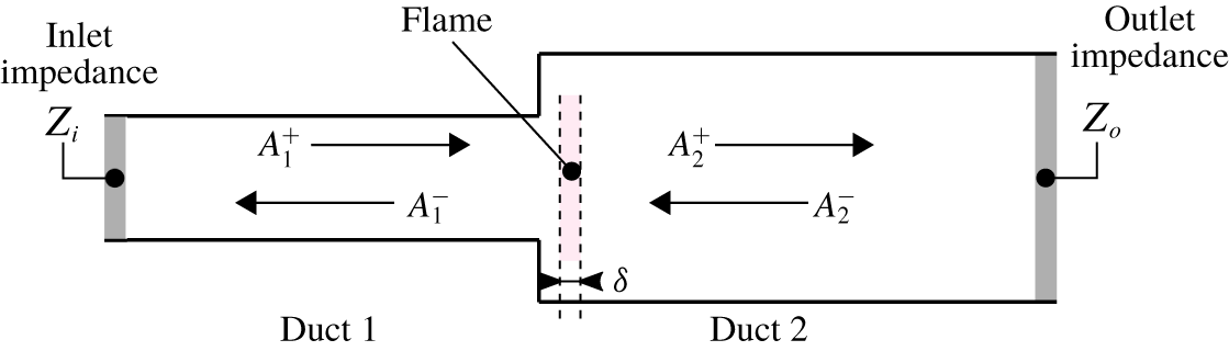
Figure 4. A schematic view of combustion instability network models: one-dimensional acoustic waves travel in a series of ducts. A compact flame is located in one section of the ducts. Inlet and outlet are characterized by their impedances.
A convenient notation to describe acoustic variables during CIs is the following. Any variable  $a$, pressure, velocity, density or temperature, is decomposed into a time average value $\bar{a}$ and a small perturbation $a^{\prime }$: $a=\overline{a}+a^{\prime }$. The analysis is usually performed by assuming harmonic variations, or a sum of harmonic variations, at an angular frequency $\unicode[STIX]{x1D714}$. The perturbation $a^{\prime }$ is written as $a^{\prime }=\text{Re}[\tilde{a}\exp (-\text{i}\unicode[STIX]{x1D714}t)]$ where $i^{2}=-1$ and $\text{Re}$ designates the real part of a complex number. All derivations are carried out using the complex equivalent of $a^{\prime }$ which is $\tilde{a}$ to simplify the algebra. Once $\tilde{a}$ is obtained, $a^{\prime }$ is deduced by taking the real part of $\tilde{a}\exp (-\text{i}\unicode[STIX]{x1D714}t)$. It is often necessary to calculate the average over a period $T=2\unicode[STIX]{x03C0}/\unicode[STIX]{x1D714}$ of a product of harmonic perturbations. Such averages appear for example in the determination of acoustic energies or fluxes:
 $$\begin{eqnarray}\displaystyle J=\frac{1}{T}\int _{0}^{T}a^{\prime }b^{\prime }\,\text{d}t. & & \displaystyle\end{eqnarray}$$
 Some straightforward calculations indicate that it is possible to express this quantity in terms of the complex amplitudes  $\tilde{a}$ and $\tilde{b}$,
 $$\begin{eqnarray}J={\textstyle \frac{1}{2}}\text{Re}(\tilde{a}\tilde{b}^{\ast })={\textstyle \frac{1}{2}}\text{Re}(\tilde{a}^{\ast }\tilde{b}),\end{eqnarray}$$
 where  $\tilde{a}^{\ast }$ is the complex conjugate of $\tilde{a}$. For example, the level of oscillation in a combustor is often measured through the root-mean-square value $p_{rms}^{\prime }$ of the pressure fluctuation. This is deduced by taking the square root of $p^{\prime 2}$ averaged over the oscillation period
 $$\begin{eqnarray}\displaystyle p_{rms}^{\prime 2}=\frac{1}{T}\int _{0}^{T}p^{\prime 2}\,\text{d}t=\frac{1}{2}\text{Re}(\,\tilde{p}\tilde{p}^{\ast }), & & \displaystyle\end{eqnarray}$$
where use has been made of Parseval’s identity.
2.1.2 Generic form for acoustic perturbations
The longitudinal acoustic field in a duct comprises two travelling waves that are planar and propagate in opposite axial directions. These waves are also isentropic since the only place where entropy changes is in the flame zone which is here considered to be compact. Therefore, in all duct elements composing a combustion system, acoustic perturbations can be decomposed in right (indexed  $^{+}$) and left (indexed $^{-}$) travelling waves obeying to the Helmholtz equation. Using the complex notation of the previous section, one has
 $$\begin{eqnarray}\displaystyle & \displaystyle p^{\prime }(x,t)=\text{Re}([A^{+}\text{e}^{\text{i}kx}+A^{-}\text{e}^{-\text{i}kx}]\text{e}^{-\text{i}\unicode[STIX]{x1D714}t}), & \displaystyle\end{eqnarray}$$
 $$\begin{eqnarray}\displaystyle & \displaystyle \bar{\unicode[STIX]{x1D70C}}cu^{\prime }(x,t)=\text{Re}([A^{+}\text{e}^{\text{i}kx}-A^{-}\text{e}^{-\text{i}kx}]\text{e}^{-\text{i}\unicode[STIX]{x1D714}t}). & \displaystyle\end{eqnarray}$$
 In (2.4), the wavenumber  $k$ may be deduced from the angular frequency and the speed of sound: $k=\unicode[STIX]{x1D714}/c$. The wave amplitudes $A^{+}$ and $A^{-}$ are determined using two types of information:
(i) The first are the boundary conditions at both ends of the system, which are usually specified by impedances as described in § 2.2. They are defined in the Fourier space and link the acoustic pressure to acoustic velocity at the boundaries.
(ii) The acoustic wavelength being large with respect to abrupt changes of the cross-section area and the flame length scales, one may link the acoustic variables by jump conditions in planes where the cross-section changes or where a flame is located as discussed in § 2.3.
One of the difficulties of combustion stability analysis is to specify impedances at the inflow and outflow boundaries and to express jump conditions at the flame reflecting the combustion response to incoming perturbations. These items are successively considered in what follows.
2.2 Impedances and admittances
The acoustic impedance is usually defined as the ratio of the pressure perturbation to the normal acoustic velocity  $Z=\tilde{p}/(\tilde{\boldsymbol{u}}\boldsymbol{\cdot }\boldsymbol{n})$ (Morse & Ingard Reference Morse and Ingard1986). In the general case, it is important to remember that the normal $\boldsymbol{n}$ is an outwards oriented unit vector. In the one-dimensional case, it is more convenient to use the velocity component in the axial direction and simply define the acoustic impedance as the ratio $Z=\tilde{p}/\tilde{u}$. The evaluation of $Z$ is simple only in a few cases. For example, on a rigid wall, the velocity perturbations are zero and the impedance $Z$ is infinite. For a duct exhausting gases into an open atmosphere, the pressure fluctuation is nearly zero at the duct open end $p^{\prime }\simeq 0$ and the impedance $Z$ is close to zero at that boundary. For all other cases, the evaluation of impedances is not as straightforward.

Figure 5. Inlet  $Z_{c}$ (compressor) and outlet $Z_{c}$ (turbine) impedances for a gas turbine engine.
It is especially complicated for engines where the combustion chamber is fed by a compressor and blows into a turbine as illustrated in figure 5. In such a situation, the determination of the compressor and turbine impedances is a problem in itself. And without knowing their values, assessing the dynamic stability of the combustion system is subject to uncertainty. For the idealized systems discussed in the present article, finding impedances is somewhat easier.
In many derivations, working with a specific impedance  $\unicode[STIX]{x1D701}$ is more convenient because it is a dimensionless complex number defined by $\unicode[STIX]{x1D701}=Z/(\unicode[STIX]{x1D70C}c)=\tilde{p}/(\unicode[STIX]{x1D70C}c\tilde{u} )$, where $\unicode[STIX]{x1D70C}c$ is the characteristic impedance of the gaseous mixture. One also defines a specific admittance as the inverse of the specific impedance $\unicode[STIX]{x1D6FD}=1/\unicode[STIX]{x1D701}=\unicode[STIX]{x1D70C}c\tilde{u} /\tilde{p}$. This definition may be used in combination with the linearized momentum equation to express the boundary condition in the form
 $$\begin{eqnarray}\frac{\text{d}\tilde{p}}{\text{d}x}=\text{i}k\unicode[STIX]{x1D6FD}\tilde{p}.\end{eqnarray}$$
2.3 Jump conditions, FTF and FDF
One may first consider the relation which governs the level of velocity perturbations on the two sides of the flame. The analysis is carried out by assuming that the combustion region is compact in a low Mach number flow. Linearized Rankine–Hugoniot relations through the flame yield (see for example the recent analysis by Chen, Bomberg & Polifke (Reference Chen, Bomberg and Polifke2016))
 $$\begin{eqnarray}\displaystyle & \displaystyle u_{2}^{\prime }-u_{1}^{\prime }=\frac{\unicode[STIX]{x1D6FE}-1}{\bar{\unicode[STIX]{x1D70C}}c^{2}}\frac{\dot{Q}^{\prime }}{S}, & \displaystyle\end{eqnarray}$$
 $$\begin{eqnarray}\displaystyle & \displaystyle p_{2}^{\prime }-p_{1}^{\prime }=0, & \displaystyle\end{eqnarray}$$
 where  $S$ is the flame surface area, $\bar{p}$ denotes the mean pressure, $\unicode[STIX]{x1D6FE}$ is the specific heat ratio and $\dot{Q}^{\prime }$ designates heat release rate fluctuations. Note that the pressure being nearly constant across the flame region, one may also safely consider that $\bar{\unicode[STIX]{x1D70C}}c^{2}=\unicode[STIX]{x1D6FE}\overline{p}$ which is nearly constant.
The main difficulty is to relate the heat release rate to the incident disturbances. Following the same reasoning as that used in early analysis of combustion instabilities in rocket engines (Crocco Reference Crocco1951, Reference Crocco1952), the heat release rate fluctuation may be linked to the incident velocity perturbations by a time-lag model. The unsteady heat release rate  $\dot{Q}^{\prime }$ produced by the flame only depends on the delayed value of the incoming inlet velocity $u_{1}^{\prime }$:
 $$\begin{eqnarray}\displaystyle \dot{Q}^{\prime }=f(u_{1}^{\prime })=nu_{1}^{\prime }(t-\unicode[STIX]{x1D70F}), & & \displaystyle\end{eqnarray}$$
 where  $n$ is an interaction index and $\unicode[STIX]{x1D70F}$ designates a time lag. In practice, it is preferable to use a dimensionless interaction index $N$ linking the relative heat release rate fluctuations to a delayed relative velocity perturbation
 $$\begin{eqnarray}\displaystyle \frac{\dot{Q}^{\prime }}{\overline{\dot{Q}}}=f\left(\frac{u_{1}^{\prime }}{\bar{u}_{1}}\right)=N\frac{u_{1}^{\prime }(t-\unicode[STIX]{x1D70F})}{\bar{u}_{1}}\,\!, & & \displaystyle\end{eqnarray}$$
 where  $\overline{\dot{Q}}$ and $\bar{u}_{1}$ are the mean total heat release rate and the mean inlet velocity, respectively. The scaled interaction index $N$ measures the strength of the flame response to incident perturbations. Large values of $N$ characterize flames that are prone to CI. The delay $\unicode[STIX]{x1D70F}$ measures the time needed by the flame to respond to incoming perturbations originating from the upstream side. It is known that systems with delays may become unstable. In combustion systems the time lag $\unicode[STIX]{x1D70F}$ often defines regions of instability by controlling the phase relationship between heat release rate disturbances and the acoustic field. Expression (2.10) implies that the interaction index $N$ of the flame is constant for all frequencies while the phase $\unicode[STIX]{x1D711}=\unicode[STIX]{x1D714}\unicode[STIX]{x1D70F}$ changes linearly with frequency.
This is only a crude approximation since flames are generally more sensitive to low-frequency disturbances and their response drops down as the frequency is increased, the flame acting like a low pass filter which rapidly damps high-frequency small wavelength disturbances. This essential feature may be taken into account by introducing a FTF in which the flame response is characterized in the Fourier space by a gain  $G$ and a phase lag $\unicode[STIX]{x1D711}$ that both depend on the angular frequency $\unicode[STIX]{x1D714}$:
 $$\begin{eqnarray}{\mathcal{F}}(\unicode[STIX]{x1D714})=\frac{\widetilde{\dot{Q}}/\overline{\dot{Q}}}{\tilde{u} _{1}/\overline{u_{1}}}=G(\unicode[STIX]{x1D714})\exp [\text{i}\unicode[STIX]{x1D711}(\unicode[STIX]{x1D714})].\end{eqnarray}$$
 The quantities  $\overline{\dot{Q}}$ and $\overline{u}_{1}$ denote the mean heat release rate and the bulk velocity at the injector outlet section.
The FTF can be extended to accommodate nonlinear features into a FDF framework. The describing function is widely used in control systems theory to represent nonlinear systems by making use of a family of transfer functions depending on the amplitude of the input. This concept was used in a theoretical analysis of the dynamics of a ducted flame (Dowling Reference Dowling1999). Using a measured FDF  ${\mathcal{F}}(\unicode[STIX]{x1D714},|\tilde{u} _{1}|)$ it was shown by Noiray et al. (Reference Noiray, Durox, Schuller and Candel2008) that many nonlinear features observed experimentally could be predicted theoretically. The FDF in combination with an acoustic analysis allowed predictions of limit cycle amplitudes, resonant frequency shifting, mode switching, instability triggering and hysteresis all in good agreement with experiments. The present analysis is here voluntarily restricted to the linear regime of vanishingly small perturbation levels $|\tilde{u} _{1}|$. Effects of finite levels of oscillation are documented for example in Noiray et al. (Reference Noiray, Durox, Schuller and Candel2008), Palies et al. (Reference Palies, Durox, Schuller and Candel2011), Krebs et al. (Reference Krebs, Krediet, Portillo, Hermeth, Poinsot, Schimek and Paschereit2013), Ghirardo, Juniper & Moeck (Reference Ghirardo, Juniper and Moeck2016) and Larea et al. (Reference Larea, Schuller, Prieur, Durox, Camporeale and Candel2017).
Two limits are useful to mention for the FTF or FDF gain  $G$. In the low-frequency limit, quasi-steady combustion takes place and the flame instantaneously converts the reactive mixture it receives ( $\dot{Q}\propto u$). As a consequence $G$ tends in this limit to unity (Polifke & Lawn Reference Polifke and Lawn2007)
 $$\begin{eqnarray}\displaystyle \text{lim}_{\unicode[STIX]{x1D714}\rightarrow 0}G=1. & & \displaystyle\end{eqnarray}$$
 This property is often used to verify the quality of FTF measurements or reconstruction from time series data. In the high-frequency limit,  $G$ drops to zero. Flames act as low-pass filters systems and high frequency modulations do not induce a finite response:
 $$\begin{eqnarray}\displaystyle \text{lim}_{\unicode[STIX]{x1D714}\rightarrow \infty }G=0. & & \displaystyle\end{eqnarray}$$
 Between these two limits, the FTF gain  $G$ can take finite values. Maximum values of the order of 2–5 are observed in some laminar flame experiments (Durox et al. Reference Durox, Schuller, Noiray and Candel2009). One may then rewrite (2.7) in Fourier space:
 $$\begin{eqnarray}\tilde{u} _{2}=\tilde{u} _{1}(1+\unicode[STIX]{x1D703}{\mathcal{F}}(\unicode[STIX]{x1D714})).\end{eqnarray}$$
 In the previous expression, use has been made of  $\widetilde{\dot{Q}}=(\overline{\dot{Q}}/\overline{u}_{1})\,{\mathcal{F}}(\unicode[STIX]{x1D714})\tilde{u} _{1}$. The parameter $\unicode[STIX]{x1D703}$ in (2.14) stands for
 $$\begin{eqnarray}\unicode[STIX]{x1D703}=\frac{\unicode[STIX]{x1D6FE}-1}{\unicode[STIX]{x1D6FE}}\frac{\overline{\dot{Q}}}{S\overline{p}\,\overline{u}_{1}}=\frac{Y_{f}(-\unicode[STIX]{x0394}h_{f}^{0})}{c_{p}T_{1}}=\frac{T_{2}}{T_{1}}-1\geqslant 0.\end{eqnarray}$$
 This dimensionless number depends on the ratio of the total heat release rate to the surface area  $\overline{\dot{Q}}/S$ indicating that the mean power flux essentially controls this relation. The mean pressure in the chamber also intervenes and $\overline{\dot{Q}}/(\overline{p}S)$ has dimensions of a velocity that needs to be compared to the bulk velocity $\bar{u}_{1}$ of the flow feeding the combustion region. This quantity may alternatively be expressed as the ratio of the energy released by combustion and the sensible enthalpy of the incoming flow, where $Y_{f}$ is the fuel mass fraction, $-\unicode[STIX]{x0394}h_{f}^{0}$ the fuel heating value, $c_{p}$ the specific heat and $T_{1}$ the temperature of the incoming flow. Finally, it may also be viewed as the relative heat produced by combustion $\unicode[STIX]{x1D703}=T_{2}/T_{1}-1$.
2.4 Approaches to study combustion instability and instability criteria
There are three main types of approaches used to analyse CI problems:
(i) Approach 1a consists in solving a set of linearized equations describing the system dynamics governing the perturbed combustion process and the coupled acoustic motion. Analytical solution is sometimes possible but in most cases the system is integrated in the time domain.
(ii) Approach 1b relies on the derivation of a dispersion relation in the frequency domain. Nonlinear terms may be treated by making use of describing function concepts and only retaining the first harmonic term. The complex roots of the dispersion relation are then sought to examine the stability of the system and see if a given acoustic mode will be amplified or damped.
(iii) Approach 2 is based on energy considerations that are used to derive stability criteria. This approach does not generally provide the full solution, but may be used to determine the growth rate of unstable modes as described later.
To illustrate these three approaches, it is instructive to begin by a simple mass/spring oscillator system where  $m$,
$m$,  $k$ and $x$ are respectively the mass, spring strength and position of the oscillating mass. A force $F$ is exerted on this system. In coupled systems this force depends on the position $x$ and velocity ${\dot{x}}$ and we assume for simplicity that this relation is linear
 $$\begin{eqnarray}m\frac{\text{d}^{2}x}{\text{d}t^{2}}+kx=F(x,{\dot{x}}).\end{eqnarray}$$
 In approach 1a, (2.16) is solved analytically or numerically by integrating from an initial state  $x(0)=x_{0}$, ${\dot{x}}(0)={\dot{x}}_{0}$. Under some conditions the system may be led to oscillate at an angular frequency $\unicode[STIX]{x1D714}$ that is close to the eigenfrequency $\unicode[STIX]{x1D714}_{0}=(k/m)^{1/2}$.
In approach 1b, the system is described in frequency space. The time derivative is replaced by  $-\text{i}\unicode[STIX]{x1D714}$. This yields a dispersion relation of the form $-m\unicode[STIX]{x1D714}^{2}+k=F(1,-\text{i}\unicode[STIX]{x1D714})$. The roots of this equation may then be determined numerically or by considering that $F$ is small and by making use of a perturbation expansion.
In approach 2, one makes no attempt to obtain a solution. The objective is instead to derive a stability criterion by examining the total energy in the system. This is obtained by multiplying (2.16) by  ${\dot{x}}$ and integrating the result. One obtains
 $$\begin{eqnarray}\displaystyle \frac{\text{d}E}{\text{d}t}=F{\dot{x}}, & & \displaystyle\end{eqnarray}$$
 where  $E$ is the total energy in the system
 $$\begin{eqnarray}E={\textstyle \frac{1}{2}}m{\dot{x}}^{2}+{\textstyle \frac{1}{2}}kx^{2}.\end{eqnarray}$$
 In the absence of external forcing  $F=0$, (2.17) indicates that the energy $E$ is constant. Oscillations will continue with the same energy. This result does not provide the position $x(t)$ but only expresses the conservation of energy. If there is a force $F$ applied to the system approaches 1a or 1b cannot be used if details controlling the force $F$ are not known. Approach 2, however, indicates that
 $$\begin{eqnarray}E(t)-E_{0}=\left[\frac{1}{2}m{\dot{x}}^{2}+\frac{1}{2}kx^{2}\right]_{0}^{t}=\int _{0}^{t}F{\dot{x}}\,\text{d}t,\end{eqnarray}$$
 which shows that the energy  $E$ of the system will grow in time if the term $\int F{\dot{x}}\,\text{d}t$ is positive or if the force $F$ is in phase with the velocity ${\dot{x}}$. This is an incomplete solution of the problem but it is useful because it provides a stability criterion. The details of the force $F$ are not needed to assess the stability of the system. This forced oscillator is stable if $\int F{\dot{x}}\,\text{d}t$ remains negative. For a swing for example, this means that pushing the swing ( $F>0$) when its velocity is positive ( ${\dot{x}}>0$) amplifies its oscillations and vice versa.
This simple example can be directly extrapolated to thermoacoustic problems. While the full solution following approach 1 of combustion oscillations is difficult to derive in many cases because the combustion response is not well known, it is still possible to construct a stability criterion similar to  $\int F{\dot{x}}\,\text{d}t<0$. This is often used to analyse the dynamic stability and determine possible control strategies.
Approach 1 is illustrated in § 2.5 in a simple case where a flame is stabilized in a duct. This is analysed by making use of a few simplifications. Section 2.6 shows how a stability criterion similar to that obtained previously can be derived for thermoacoustics and discusses two examples of application.
2.5 Approach 1: longitudinal thermoacoustics in a channel
The model problem illustrated in figure 6 is examined in what follows by making use of approach 1. A flame is stabilized in a duct at a sudden expansion of the cross-section separating the injection unit (length  $l_{1}$, section $S_{1}$) from the combustion chamber (length $l_{2}$, section $S_{2}$). The objective is to determine whether the flame can couple to longitudinal acoustic modes of the system. The analysis is limited to low-frequency acoustic waves for which the wavelength, typically of the order of a metre, is much greater than the flame length. The flame is ‘compact’ and can be treated as a discontinuity between fresh and burnt gases.

Figure 6. A model for combustion instabilities: a laminar flame is stabilized at the plane  $x=0$ separating an injection duct (length $l_{1}$) and a combustion chamber (length $l_{2}$). The field plotted in colour corresponds to the velocity modulus (Courtine, Selle & Poinsot Reference Courtine, Selle and Poinsot2015). Here $A_{i}^{+}$ and $A_{i}^{-}$ are the acoustic right- and left-going waves in duct $i$, respectively.
Under these assumptions, plane acoustic waves propagate in the injection tube and in the chamber, which are respectively numbered  $j=1$ and $2$. The compact flame is located at $x=0$. The fluctuating acoustic pressures $p_{j}^{\prime }$ and velocities $u_{j}^{\prime }$ in these two ducts are
 $$\begin{eqnarray}\displaystyle & \displaystyle \bar{\unicode[STIX]{x1D70C}}_{j}c_{j}u_{j}^{\prime }(x,t)=\text{Re}([A_{j}^{+}\text{e}^{\text{i}k_{j}x}-A_{j}^{-}\text{e}^{-\text{i}k_{j}x}]\text{e}^{-\text{i}\unicode[STIX]{x1D714}t}), & \displaystyle\end{eqnarray}$$
 $$\begin{eqnarray}\displaystyle & \displaystyle p_{j}^{\prime }(x,t)=\text{Re}([A_{j}^{+}\text{e}^{\text{i}k_{j}x}+A_{j}^{-}\text{e}^{-\text{i}k_{j}x}]\text{e}^{-\text{i}\unicode[STIX]{x1D714}t}), & \displaystyle\end{eqnarray}$$
 where  $k_{j}=\unicode[STIX]{x1D714}/c_{j}$ is the wavenumber in duct $j$,
$j$,  $\unicode[STIX]{x1D714}$ the angular frequency and $c_{j}$ the speed of sound in duct $j$. Since the problem involves four unknown quantities, the wave amplitudes $A_{1}^{+}$, $A_{2}^{+}$, $A_{1}^{-}$ and $A_{2}^{-}$, four conditions are needed:
(i) One boundary condition is given at the inlet at $x=-l_{1}$ and one at the outlet at $x=l_{2}$. Very often $u_{1}^{\prime }=0$ is applied at $x=-l_{1}$ because one assumes that velocity is imposed at the inlet corresponding to an infinite impedance $Z_{i}\rightarrow \infty$. The outlet is open to the ambient atmosphere and one may consider that $p^{\prime }=0$ at $x=l_{2}$. This corresponds to a vanishing impedance $Z_{o}=0$ at the open end of the duct.
(ii) Two conditions are expressed across the flame itself. At the plane
$x=0$ where the flame is stabilized, jump conditions from one side of the flame to the other relate pressure and velocity perturbations, assuming that the flame is compact compared to the acoustic wavelength. Such conditions were introduced previously. They express the continuity of pressure and the change of acoustic volume flow rate due the unsteady heat release in the flame $\dot{Q}^{\prime }$ (Crighton et al. Reference Crighton, Dowling, Ffowcs Williams, Heckl and Leppington1992; Poinsot & Veynante Reference Poinsot and Veynante2012): (2.22a,b)where$$\begin{eqnarray}p_{2}^{\prime }(x=0,t)=p_{1}^{\prime }(x=0,t)\quad \text{and}\quad S_{2}u_{2}^{\prime }(x=0,t)=S_{1}u_{1}^{\prime }(x=0,t)+\frac{\unicode[STIX]{x1D6FE}-1}{\unicode[STIX]{x1D70C}_{1}c_{1}^{2}}\dot{Q}^{\prime },\end{eqnarray}$$$\bar{\unicode[STIX]{x1D70C}}_{j}$ is the mean density in section $j$ and $\unicode[STIX]{x1D6FE}$ the ratio of specific heats. The construction of jump conditions at a compact flame front when the Mach number tends to zero, is actually an open topic which is beyond the objective of the present article. Readers are referred to recent papers by Bauerheim, Nicoud & Poinsot (Reference Bauerheim, Nicoud and Poinsot2015) and Chen et al. (Reference Chen, Bomberg and Polifke2016) on this subject.


The unsteady heat release rate  $\dot{Q}^{\prime }$ is then expressed using the time-lag model defined in (2.10) in which $N$ and $\unicode[STIX]{x1D70F}$ are assumed to be constant:
 $$\begin{eqnarray}\frac{\unicode[STIX]{x1D6FE}-1}{\bar{\unicode[STIX]{x1D70C}}_{1}c_{1}^{2}S_{1}}\dot{Q}^{\prime }=N(\unicode[STIX]{x1D703}-1)u_{1}^{\prime }(x=0,t-\unicode[STIX]{x1D70F}),\end{eqnarray}$$
 where  $\unicode[STIX]{x1D703}=T_{2}/T_{1}-1$ measures the relative change in sensible enthalpy released within the flow by combustion. Assuming harmonic variations for all perturbations $a^{\prime }=\tilde{a}\text{e}^{-\text{i}\unicode[STIX]{x1D714}t}$, the jump conditions become
 $$\begin{eqnarray}\tilde{p}_{2}(x=0,t)=\tilde{p}_{1}(x=0,t)\quad \text{and}\quad S_{2}\tilde{u} _{2}(x=0,t)=S_{1}\tilde{u} _{1}(x=0,t)(1+\unicode[STIX]{x1D703}N\text{e}^{\text{i}\unicode[STIX]{x1D714}\unicode[STIX]{x1D70F}}).\end{eqnarray}$$
 Equation (2.23) links heat release rate fluctuations to the acoustic velocity at the chamber inlet  $x=0$. The previous jump conditions together with the boundary conditions expressing that the velocity and pressure, respectively, vanish at the inlet and outlet
 $$\begin{eqnarray}\displaystyle & \displaystyle A_{1}^{+}\text{e}^{-\text{i}k_{1}l_{1}}-A_{1}^{-}\text{e}^{\text{i}k_{1}l_{1}}=0, & \displaystyle\end{eqnarray}$$
 $$\begin{eqnarray}\displaystyle & \displaystyle A_{2}^{+}\text{e}^{\text{i}k_{2}l_{2}}+A_{2}^{-}\text{e}^{-\text{i}k_{2}l_{2}}=0, & \displaystyle\end{eqnarray}$$
 lead to a homogeneous system of equations for the wave amplitudes  $A_{1}^{-}$, $A_{1}^{+}$, $A_{2}^{-}$ and $A_{2}^{+}$, which has a non-zero solution only if
 $$\begin{eqnarray}\cos \left(\unicode[STIX]{x1D714}\frac{l_{2}}{c_{2}}\right)\cos \left(\unicode[STIX]{x1D714}\frac{l_{1}}{c_{1}}\right)-\unicode[STIX]{x1D6EF}\sin \left(\unicode[STIX]{x1D714}\frac{l_{2}}{c_{2}}\right)\sin \left(\unicode[STIX]{x1D714}\frac{l_{1}}{c_{1}}\right)(1+\unicode[STIX]{x1D703}N\text{e}^{\text{i}\unicode[STIX]{x1D714}\unicode[STIX]{x1D70F}})=0,\end{eqnarray}$$
 where  $\unicode[STIX]{x1D6EF}=(\bar{\unicode[STIX]{x1D70C}}_{2}c_{2})/(\bar{\unicode[STIX]{x1D70C}}_{1}c_{1})(S_{1}/S_{2})$ is a coupling index between cavities upstream and downstream of the flame (Schuller et al. Reference Schuller, Durox, Palies and Candel2012). The dispersion relation (2.27) gives the complex angular frequency $\unicode[STIX]{x1D714}=\unicode[STIX]{x1D714}_{r}+\text{i}\unicode[STIX]{x1D714}_{i}$. The real part of $\unicode[STIX]{x1D714}$ fixes the angular frequency $\unicode[STIX]{x1D714}_{r}$ of the mode while its imaginary part provides the growth rate $\unicode[STIX]{x1D714}_{i}$. If this last quantity is positive, the mode will be linearly amplified, leading to CI.
The general solution of (2.27) is difficult to formulate without additional simplifications. For example, an analytical expression can be obtained in a case where the two channels have equal sections  $S_{2}=S_{1}$ and lengths $l_{2}=l_{1}=a$ and the flame induces a negligible heat release so that $\unicode[STIX]{x1D70C}_{2}\simeq \unicode[STIX]{x1D70C}_{1}$ and $c_{2}\simeq c_{1}\simeq c$. In this case, $\unicode[STIX]{x1D6EF}=1$ and $\unicode[STIX]{x1D703}$ is a small number. The dispersion relation becomes
 $$\begin{eqnarray}\cos ^{2}\left(\frac{\unicode[STIX]{x1D714}a}{c}\right)-\sin ^{2}\left(\frac{\unicode[STIX]{x1D714}a}{c}\right)(1+\unicode[STIX]{x1D703}N\text{e}^{\text{i}\unicode[STIX]{x1D714}\unicode[STIX]{x1D70F}})=0.\end{eqnarray}$$
 Without the flame,  $N=0$, the solution of the dispersion relation (2.28) corresponds to the acoustic eigenmodes of a duct of length $2a$. The first mode is such that $k_{0}a=\unicode[STIX]{x03C0}/4$ with $A_{1}^{+}=A_{2}^{+}$ and $A_{1}^{-}=A_{2}^{-}$. It has a zero growth rate $\text{Im}(k_{0})=0$ and a wavelength $\unicode[STIX]{x1D706}_{0}=2\unicode[STIX]{x03C0}/k_{0}=8a$ which is four times the total length of the duct $2a$. It is therefore designated as a ‘quarter-wave’ mode of the system. Its period is $T_{0}=2\unicode[STIX]{x03C0}/\unicode[STIX]{x1D714}_{0}=8a/c$. The associated fields of unsteady velocity and pressure are
 $$\begin{eqnarray}\displaystyle & \displaystyle \bar{\unicode[STIX]{x1D70C}}_{j}c_{j}u_{j}^{\prime }(x,t)=A_{1}^{+}\text{Re}[\text{e}^{\text{i}k_{0}x}+\text{i}\text{e}^{-\text{i}k_{0}x}]\text{e}^{-\text{i}\unicode[STIX]{x1D714}t}, & \displaystyle\end{eqnarray}$$
 $$\begin{eqnarray}\displaystyle & \displaystyle p_{j}^{\prime }(x,t)=A_{1}^{+}\text{Re}[\text{e}^{\text{i}k_{0}x}-\text{i}\text{e}^{-\text{i}k_{0}x}]\text{e}^{-\text{i}\unicode[STIX]{x1D714}t}, & \displaystyle\end{eqnarray}$$
 where  $A_{1}^{+}$ is the modal amplitude, which remains arbitrary as no information on amplitudes can be obtained in a linear framework. If the flame is present and the interaction index $N$ is non-zero but still small, the solution for $k$ can be obtained using a small perturbation expansion around $k_{0}$ so that $k=k_{0}+k^{\prime }$ with
 $$\begin{eqnarray}\text{Re}(k)=k_{0}+\text{Re}(k^{\prime })=\frac{\unicode[STIX]{x03C0}}{4a}-\frac{\unicode[STIX]{x1D703}N}{4a}\cos \!\left(\frac{2\unicode[STIX]{x03C0}\unicode[STIX]{x1D70F}}{T_{0}}\!\right)\quad \text{and}\quad \text{Im}(k)=\text{Im}(k^{\prime })=-\frac{\unicode[STIX]{x1D703}N}{4a}\sin \!\left(\frac{2\unicode[STIX]{x03C0}\unicode[STIX]{x1D70F}}{T_{0}}\!\right)\!.\end{eqnarray}$$
 For small interaction index  $N$ values, the mode wavenumber $\text{Re}(k)$ is only weakly altered by the presence of the flame and remains close to its value $f_{0}=\unicode[STIX]{x03C0}/(4a)$ for the quarter-wave mode frequency without the flame. The flame response defined by a non-zero interaction index $N\neq 0$, however, controls the growth rate of this mode. The combustor is unstable if $\text{Im}(k)>0$, which implies $\sin (2\unicode[STIX]{x03C0}\unicode[STIX]{x1D70F}/T_{0})<0$ that is obtained when
 $$\begin{eqnarray}s+1/2<\frac{\unicode[STIX]{x1D70F}}{T_{0}}<s+1,\end{eqnarray}$$
 where  $s$ is an integer. Any flame with a time delay $\unicode[STIX]{x1D70F}$ such that $(1/2+s)T_{0}<\unicode[STIX]{x1D70F}<(1+s)T_{0}$ will lead to CI in the absence of other damping mechanisms. Note also that this condition defines instability ‘bands’ for $\unicode[STIX]{x1D70F}$. Increasing $\unicode[STIX]{x1D70F}$ from zero corresponds to a stable quarter-wave mode for $\unicode[STIX]{x1D70F}<T_{0}/2$ followed by a band of instability when $T_{0}/2<\unicode[STIX]{x1D70F}<T_{0}$, followed by a new stability zone when $\unicode[STIX]{x1D70F}$ exceeds $T_{0}$ and so on… One may also note that this analysis needs to be repeated for higher-order modes. In the present case, the $3/4$, $5/4$, $7/4$ modes also have their own instability bands and the flame is stable only when $\unicode[STIX]{x1D70F}$ falls outside of all these instability bands. This may seem a difficult condition to ensure but in practice, high-order modes are also rapidly damped by various dissipation mechanisms and energy losses at the system boundaries. These mechanisms are neglected in the present analysis. It is rare to see CIs coupled to high-order modes, except for high-frequency instabilities that are often coupled by transverse modes at frequencies in excess of 1 kHz. In that case the combustion region is no longer compact but each of the flames formed by the various injectors remains compact with respect to the acoustic wavelength. In practice, there are indeed values of $\unicode[STIX]{x1D70F}$ which are stable for all modes.
Even if the assumptions made to derive the stability criterion (2.32) are crude, this analysis contains all the ingredients of many low-order models used in thermoacoustics:
(i) It requires that all convective and chemistry effects be modelled as a function of a purely acoustic quantity, which is here, the inlet flow velocity. Models linking the unsteady heat release rate
$\dot{Q}^{\prime }$ to the acoustic inlet velocity $u_{1}^{\prime }(x=0,t)$ are ubiquitous. More advanced models may be found in the literature (Paschereit et al. Reference Paschereit, Polifke, Schuermans and Mattson2002; Truffin & Poinsot Reference Truffin and Poinsot2005; Taraneh et al. Reference Taraneh, Schmid, Richecoeur and Durox2015) and two of them need to be mentioned. The first extends the FTF concept by considering that the flame response may be represented by a FDF where the gain $G$ and phase lag $\unicode[STIX]{x1D711}$, not only depend on frequency but also on the forcing amplitude $|u_{1}|$ (Noiray et al. Reference Noiray, Durox, Schuller and Candel2008; Durox et al. Reference Durox, Schuller, Noiray and Candel2009; Palies et al. Reference Palies, Durox, Schuller and Candel2011). A second extension of the flame transfer function concept was made to account for the fact that, in many systems, the fresh stream velocity may not be the only quantity inducing unsteady combustion. Fluctuations in equivalence ratio $\unicode[STIX]{x1D719}$ have been identified as another important perturbation that may affect the combustion process (Lieuwen & Zinn Reference Lieuwen and Zinn1998; Sattelmayer Reference Sattelmayer2003; Birbaud et al. Reference Birbaud, Ducruix, Durox and Candel2008). These fluctuations may be caused for example by a difference in the response of the air and fuel injection devices to incident pressure waves. It is then important to consider the flame response to equivalence ratio disturbances and this may be represented by an FDF that accounts for the two types of incident perturbations (2.33)where$$\begin{eqnarray}\frac{\widetilde{\dot{Q}}}{\overline{\dot{Q}}}=F_{1}(\unicode[STIX]{x1D714},|\tilde{u} _{1}|)\frac{\tilde{u} _{1}(x=0)}{\bar{u}_{1}(x=0)}+F_{2}(\unicode[STIX]{x1D714},|\tilde{\unicode[STIX]{x1D719}}_{1}|)\frac{\tilde{\unicode[STIX]{x1D719}}_{1}(x=0)}{\bar{\unicode[STIX]{x1D719}}_{0}(x=0)},\end{eqnarray}$$$\tilde{u} _{1}$ and $\tilde{\unicode[STIX]{x1D719}}_{1}$ are the velocity and equivalence ratio perturbations at the burnet outlet. This problem is investigated in § 6 for linear flow disturbances when the disturbance levels $|\tilde{u} _{1}|$ and $|\tilde{\unicode[STIX]{x1D719}}_{1}|$ may be considered to be small.(ii) The analysis leads to a stability criterion that depends on the time lag
$\unicode[STIX]{x1D70F}$ between heat release rate and flow rate disturbances at the burner inlet. When the wavenumber $k$ is determined, the modal structure, i.e. the shape of $p^{\prime }$ and $u^{\prime }$ as a function of the spatial coordinates, can be obtained too. As an example, figure 7 displays the structure of the first two modes, namely the $1/4$ and $3/4$ wave modes, in a duct with $u^{\prime }=0$ at the inlet and $p^{\prime }=0$ at the outlet.


Figure 7. The structure of the  $1/4$ and $3/4$ wave modes in the model of figure 6.
2.6 Approach 2: the Rayleigh criterion
The previous section was based on a full solution of the acoustic equations after a simplification of the problem in which the flame is considered to be compact and acoustic propagation is assumed to be longitudinal. This section now explores an approach of type 2 where the objective is to derive a stability criterion by writing an acoustic energy balance, analogue to the mechanical energy  $E$ defined in (2.17). This is done by starting from the Navier–Stokes equations expressed here in vector form, using material derivatives defined by
 $$\begin{eqnarray}\frac{\text{D}a}{\text{D}t}=\frac{\unicode[STIX]{x2202}a}{\unicode[STIX]{x2202}t}+\boldsymbol{u}\boldsymbol{\cdot }\unicode[STIX]{x1D735}a,\end{eqnarray}$$
 for a quantity  $a$ transported by the flow. Neglecting body forces, the momentum balance writes
 $$\begin{eqnarray}\displaystyle \unicode[STIX]{x1D70C}\frac{\text{D}\boldsymbol{u}}{\text{D}t}=-\unicode[STIX]{x1D735}p+\unicode[STIX]{x1D735}\boldsymbol{\cdot }\unicode[STIX]{x1D749}, & & \displaystyle\end{eqnarray}$$
 where  $\unicode[STIX]{x1D749}$ is the viscous stress tensor. Starting from the enthalpy (or energy) conservation equation and assuming equal specific heats for all species, negligible heat diffusion and low Mach number, a governing equation can be written for pressure (Poinsot & Veynante Reference Poinsot and Veynante2012)
 $$\begin{eqnarray}\displaystyle \frac{\unicode[STIX]{x2202}p}{\unicode[STIX]{x2202}t}=-\unicode[STIX]{x1D6FE}p\unicode[STIX]{x1D735}\boldsymbol{\cdot }\boldsymbol{u}+(\unicode[STIX]{x1D6FE}-1)\dot{q}, & & \displaystyle\end{eqnarray}$$
 where  $\dot{q}$ is the volumetric rate of heat release by the flame.
To derive an energy balance for the acoustic perturbations, (2.34) and (2.35) are linearized around a mean state in the chamber by writing
 $$\begin{eqnarray}\unicode[STIX]{x1D70C}=\bar{\unicode[STIX]{x1D70C}}+\unicode[STIX]{x1D70C}^{\prime },\quad \boldsymbol{u}=\bar{\boldsymbol{u}}+\boldsymbol{u}^{\prime }\quad \text{and}\quad p=\bar{p}+p^{\prime }.\end{eqnarray}$$
 The linearized equation for the acoustic velocity  $\boldsymbol{u}^{\prime }$ is simplified from (2.34) at low mean Mach number to yield
 $$\begin{eqnarray}\displaystyle \bar{\unicode[STIX]{x1D70C}}\frac{\unicode[STIX]{x2202}\boldsymbol{u}^{\prime }}{\unicode[STIX]{x2202}t}=-\unicode[STIX]{x1D735}p^{\prime }, & & \displaystyle\end{eqnarray}$$
 where  $\bar{\unicode[STIX]{x1D70C}}$ can be a function of space. The equation for pressure perturbations is obtained by linearizing (2.35) leading to (Crighton et al. Reference Crighton, Dowling, Ffowcs Williams, Heckl and Leppington1992; Candel, Huynh & Poinsot Reference Candel, Huynh and Poinsot1996)
 $$\begin{eqnarray}\displaystyle \frac{1}{\unicode[STIX]{x1D6FE}\bar{p}}\frac{\unicode[STIX]{x2202}p^{\prime }}{\unicode[STIX]{x2202}t}+\unicode[STIX]{x1D735}\boldsymbol{\cdot }\boldsymbol{u}^{\prime }=\frac{\unicode[STIX]{x1D6FE}-1}{\unicode[STIX]{x1D6FE}\bar{p}}\dot{q}^{\prime }, & & \displaystyle\end{eqnarray}$$
 where  $\dot{q}^{\prime }$ is a disturbance of the volumetric rate of heat release by combustion. The linearized equations (2.37) for $\boldsymbol{u}^{\prime }$ and (2.38) for $p^{\prime }$ can now be combined to form an equation for the acoustic energy in reacting flows
 $$\begin{eqnarray}\displaystyle e=\frac{1}{2}\bar{\unicode[STIX]{x1D70C}}u^{\prime 2}+\frac{1}{2}\frac{p^{\prime 2}}{\bar{\unicode[STIX]{x1D70C}}c_{0}^{2}}. & & \displaystyle\end{eqnarray}$$
 This is done by multiplying (2.38) by  $p^{\prime }$, taking the scalar product of the momentum equation (2.37) by $\boldsymbol{u}^{\prime }$ to get
 $$\begin{eqnarray}\displaystyle \frac{\unicode[STIX]{x2202}e}{\unicode[STIX]{x2202}t}+\unicode[STIX]{x1D735}\boldsymbol{\cdot }\boldsymbol{f}=r,\quad \text{with }r=\frac{(\unicode[STIX]{x1D6FE}-1)}{\unicode[STIX]{x1D6FE}\bar{p}}p^{\prime }\dot{q}^{\prime }\;\text{and}\;\,\boldsymbol{f}=p^{\prime }\boldsymbol{u}^{\prime }. & & \displaystyle\end{eqnarray}$$
 The source term  $r$ features the product of the local unsteady pressure $p^{\prime }$ with the unsteady rate of heat release $\dot{q}^{\prime }$ in the flame. This yields a stability criterion that is similar to that obtained for a simple mass spring oscillator. When $r$ is positive, i.e. if the pressure oscillations $p^{\prime }$ are in phase with the unsteady volumetric rate of heat release $\dot{q}^{\prime }$, $r$ increases the acoustic energy and the instability is locally amplified. On the other hand, if the volumetric rate of unsteady heat release is maximum when pressure is minimum, the instability decreases. This criterion for combustion instability was first proposed by Rayleigh (Reference Rayleigh1878). The index $r$ changes with time and location. Some regions excite the oscillation by burning in phase with pressure leading to positive $r$ values while others damp the instability by burning out of phase with pressure (Poinsot et al. Reference Poinsot, Trouvé, Veynante, Candel and Esposito1987; Samaniego et al. Reference Samaniego, Yip, Poinsot and Candel1993).
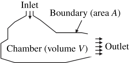
Figure 8. Control volume for energy balance in a typical combustion chamber.
The overall effect of flame/acoustics coupling can only be predicted by integrating (2.40) over space and time. Consider a typical combustion chamber as in figure 8. Integration of the local energy balance (2.40) over the whole combustor volume  $V$ surrounded by surface $A$ yields
 $$\begin{eqnarray}\displaystyle \frac{\text{d}}{\text{d}t}\int _{V}e\,\text{d}V+\int _{A}\boldsymbol{f}\boldsymbol{\cdot }\boldsymbol{n}\,\text{d}A=\int _{V}r\,\text{d}V, & & \displaystyle\end{eqnarray}$$
 where  $\boldsymbol{n}$ is the local normal vector to the surface $A$. In (2.41), all terms are time dependent. The acoustic flux term $\boldsymbol{f}\boldsymbol{\cdot }\boldsymbol{n}$ is usually zero at all walls but may differ from zero at the inlet and outlet sections. It indicates how much of the acoustic energy produced in the combustor is lost at the boundaries.
To provide meaningful information on the growth of the instability, expression (2.41) must also be averaged over time. For harmonic oscillations, this can be done over a period of oscillation  $T$ (see table 1 for notations):
 $$\begin{eqnarray}\displaystyle p^{\prime }=\text{Re}(\tilde{p}(t)\text{e}^{-\text{i}\unicode[STIX]{x1D714}t}),\quad \boldsymbol{u}^{\prime }=\text{Re}(\tilde{\boldsymbol{u}}(t)\text{e}^{-\text{i}\unicode[STIX]{x1D714}t})\quad \text{and}\quad \dot{q}^{\prime }=\text{Re}(\widetilde{\dot{q}}(t)\text{e}^{-\text{i}\unicode[STIX]{x1D714}t}), & & \displaystyle\end{eqnarray}$$
 where  $\tilde{p}(t)$, $\tilde{\boldsymbol{u}}(t)$ and $\widetilde{\dot{q}}(t)$ are slowly varying functions over a time scale $t$ much longer than the acoustic period $T$. Whether these functions grow with time for a given angular frequency $\unicode[STIX]{x1D714}$ determines the stability of the combustor. Integrating (2.41) over a period of oscillation $T=2\unicode[STIX]{x03C0}/\unicode[STIX]{x1D714}$ and dividing by $T$ yields
 $$\begin{eqnarray}\displaystyle \frac{\text{d}}{\text{d}t}{\mathcal{E}}+{\mathcal{D}}={\mathcal{R}}, & & \displaystyle\end{eqnarray}$$
 where  ${\mathcal{E}}$ is the period-averaged acoustic energy in the whole combustor
 $$\begin{eqnarray}\displaystyle {\mathcal{E}}=\int _{V}E\,\text{d}V\quad \text{and}\quad E=\frac{1}{T}\int _{0}^{T}e\,\text{d}t=\frac{1}{4\bar{\unicode[STIX]{x1D70C}}c^{2}}\tilde{p}\tilde{p}^{\ast }+\frac{1}{4}\bar{\unicode[STIX]{x1D70C}}\tilde{\boldsymbol{u}}\boldsymbol{\cdot }\tilde{\boldsymbol{u}}^{\ast }. & & \displaystyle\end{eqnarray}$$
The period-averaged acoustic flux leaving the combustor is
 $$\begin{eqnarray}\displaystyle {\mathcal{D}}=\int _{A}F\,\text{d}A\quad \text{and}\quad F=\frac{1}{T}\int _{0}^{T}\boldsymbol{f}\boldsymbol{\cdot }\boldsymbol{n}\,\text{d}t=\frac{1}{2}\text{Re}(\tilde{p}\tilde{\boldsymbol{u}}^{\ast })\boldsymbol{\cdot }\boldsymbol{n}=\frac{1}{2}\text{Re}(Z)\tilde{\boldsymbol{u}}\boldsymbol{\cdot }\tilde{\boldsymbol{u}}^{\ast }.\qquad & & \displaystyle\end{eqnarray}$$
 The latter expression exhibits the impedance  $Z=\tilde{p}/(\tilde{\boldsymbol{u}}\boldsymbol{\cdot }\boldsymbol{n})$ at the inlets and outlets, highlighting their effects on acoustic losses.
Finally, the average source term is
 $$\begin{eqnarray}\displaystyle {\mathcal{R}}=\int _{V}R\,\text{d}V\quad \text{and}\quad R=\frac{1}{T}\int _{0}^{T}r\,\text{d}t=\frac{(\unicode[STIX]{x1D6FE}-1)}{T\unicode[STIX]{x1D6FE}\bar{p}}\int _{0}^{T}p^{\prime }\dot{q}^{\prime }\,\text{d}t=\frac{(\unicode[STIX]{x1D6FE}-1)}{2\unicode[STIX]{x1D6FE}\bar{p}}\text{Re}(\tilde{p}\widetilde{\dot{q}}^{\ast }). & & \displaystyle \nonumber\\ \displaystyle & & \displaystyle\end{eqnarray}$$
 Flame/acoustic coupling now appears in the  ${\mathcal{R}}$ term. This space-averaged integral over the combustor volume $V$ of the period-averaged value of $\tilde{p}\widetilde{\dot{q}}^{\ast }$ must be positive to increase the acoustic energy of the oscillation.
Table 1. Definitions of acoustic energies, fluxes and source terms.
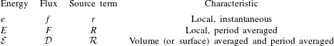
The growth rate  $\unicode[STIX]{x1D714}_{i}$ of the acoustic energy may now be deduced. It is expressed by assuming that the perturbation amplitudes change slowly with time in comparison to acoustic times so that $\tilde{p}$, $\tilde{\boldsymbol{u}}$ and $\widetilde{\dot{q}}$ functions may be written
 $$\begin{eqnarray}\displaystyle \tilde{p}(t)=\hat{p}\text{e}^{\unicode[STIX]{x1D714}_{i}t},\quad \tilde{\boldsymbol{u}}=\hat{\boldsymbol{u}}\text{e}^{\unicode[STIX]{x1D714}_{i}t},\quad \text{and}\quad \widetilde{\dot{q}}(t)=\hat{\dot{q}}\text{e}^{\unicode[STIX]{x1D714}_{i}t}, & & \displaystyle\end{eqnarray}$$
 where  $\unicode[STIX]{x1D714}_{i}T\ll 1$. The energy balance (2.43) becomes in this case
 $$\begin{eqnarray}\displaystyle \unicode[STIX]{x1D714}_{i}=({\mathcal{R}}-{\mathcal{D}})/(2{\mathcal{E}}). & & \displaystyle\end{eqnarray}$$
 The growth rate  $\unicode[STIX]{x1D714}_{i}$ is the difference between the combustion source term ${\mathcal{R}}$ and the acoustic losses ${\mathcal{D}}$ at the boundaries. Equation (2.48) can be interpreted as a generalized Rayleigh criterion. Combustion becomes unstable when $\unicode[STIX]{x1D714}_{i}>0$ meaning that from energetic consideration the instability criterion is
 $$\begin{eqnarray}\displaystyle {\mathcal{R}}>{\mathcal{D}}. & & \displaystyle\end{eqnarray}$$
 At this point it is interesting to connect this analysis to the example investigated in § 2.5 and sketched in figure 6. In this example, the flame is assumed to have a negligible feedback on the mean flow because the interaction index  $N$ is small, so that, for the quarter wave mode for example, the pressure fluctuations $p^{\prime }$ at the flame front and the unsteady rate of heat release $\dot{Q}^{\prime }$ are given by
 $$\begin{eqnarray}\displaystyle & \displaystyle \dot{Q}^{\prime }(t)\propto u_{1}^{\prime }(x=0,t-\unicode[STIX]{x1D70F})=A_{1}^{+}\frac{1}{\unicode[STIX]{x1D70C}_{1}c_{1}}\text{Re}[(\text{e}^{\text{i}k_{0}x}+\text{i}\text{e}^{-\text{i}k_{0}x})\text{e}^{-\text{i}\unicode[STIX]{x1D714}(t-\unicode[STIX]{x1D70F})}], & \displaystyle\end{eqnarray}$$
 $$\begin{eqnarray}\displaystyle & \displaystyle p^{\prime }(x=0,t)=A_{1}^{+}\text{Re}[(\text{e}^{\text{i}k_{0}x}-\text{i}\text{e}^{-\text{i}k_{0}x})\text{e}^{-\text{i}\unicode[STIX]{x1D714}t}]. & \displaystyle\end{eqnarray}$$
For this compact flame, the Rayleigh criterion can be formed by taking the product of these two quantities. Its averaged value over time is
 $$\begin{eqnarray}\displaystyle {\mathcal{R}}=\frac{(\unicode[STIX]{x1D6FE}-1)}{2\unicode[STIX]{x1D6FE}\bar{p}}\text{Re}(\tilde{p}\widetilde{\dot{Q}}^{\ast })\propto -\frac{(\unicode[STIX]{x1D6FE}-1)}{\unicode[STIX]{x1D6FE}\bar{p}}A_{1+}^{2}\sin (\unicode[STIX]{x1D714}\unicode[STIX]{x1D70F}). & & \displaystyle\end{eqnarray}$$
 CI only develop when  $\sin (\unicode[STIX]{x1D714}\unicode[STIX]{x1D70F})<0$ which is the criterion obtained by making use of approach 1 in the previous section. As announced, both methods provide similar stability criteria. Approach 1 provides the full solution, while approach 2 requires some knowledge on the acoustic $\boldsymbol{u}^{\prime }$ and $p^{\prime }$ fields and only provides a stability criterion.
A last example combining all notions presented in this tutorial is given. Consider a burner of any shape where an injection system feeds a combustion chamber in which a compact flame is stabilized as in figure 4. The compact flame response to incoming flow-rate disturbances is modelled by a time-lag model  $\dot{Q}^{\prime }\propto nu^{\prime }(t-\unicode[STIX]{x1D70F})$. If the impedance of the injection system (at the cross-section area expansion in figure 4) is characterized by $Z=|Z|\text{e}^{\text{i}\unicode[STIX]{x1D6E9}}$, the Rayleigh criterion provides a useful description of the physics of CIs in this system. The Rayleigh term ${\mathcal{R}}\propto 1/T\int _{0}^{T}p^{\prime }\dot{Q}^{\prime }\,\text{d}t$ is
 $$\begin{eqnarray}\displaystyle {\mathcal{R}}\propto \frac{1}{T}\int _{0}^{T}p^{\prime }nu^{\prime }(t-\unicode[STIX]{x1D70F})\,\text{d}t=\frac{1}{2}\text{Re}[|Z|\tilde{u} \tilde{u} ^{\ast }n\text{e}^{\text{i}(\unicode[STIX]{x1D719}-\unicode[STIX]{x1D714}\unicode[STIX]{x1D70F})}]=\frac{1}{2}|Z||\tilde{u} |^{2}n\cos (\unicode[STIX]{x1D6E9}-\unicode[STIX]{x1D714}\unicode[STIX]{x1D70F}),\quad & & \displaystyle\end{eqnarray}$$
 which shows that the stability of the chamber in figure 4 is controlled by the difference between the injector phase  $\unicode[STIX]{x1D6E9}$ and that corresponding to the time delay in the flame response $\unicode[STIX]{x1D714}\unicode[STIX]{x1D70F}$. This simple example illustrates a major result of CI studies. The stability of a combustor does not depend on the flame delay $\unicode[STIX]{x1D70F}$ only, but is also controlled by the injector impedance phase lag $\unicode[STIX]{x1D6E9}$. A combustion chamber can be stable when it is equipped with one injection system and unstable when another injection system is installed.
Approach 1 is generalized in the next section and applied to a series of canonical configurations.
3 Axial modes in laminar burners
The main objective of this section is to provide a theoretical framework allowing us to get analytical results that may serve as guidelines in a variety of practical configurations. The development essentially follows approach 1 lines of reasoning. The results obtained are particularly useful when measured or calculated FTFs are available (Schuller, Durox & Candel Reference Schuller, Durox and Candel2003a). It is shown that the model in conjunction with a flame transfer function yields insights on conditions leading to instability and their growth rates as can be tested in axial set-ups or in annular combustor experiments.
One again considers low-frequency one-dimensional acoustic waves propagating in ducts and interacting with a compact unsteady flame sheet as in the tutorial section. The objective is to generalize the expression (2.27) to other system geometries with more complex boundary conditions and with an improved description of the flame response to flow perturbations. It is then shown how to determine the oscillation frequency of CIs and their growth rates with a new method disregarding the feedback from acoustics on the flame dynamics. This methodology leads to drastic simplifications of the stability analysis and its validity domain is assessed.

Figure 9. Flame sheet interacting with upstream and downstream acoustic waves represented by their admittances.
The system dynamics may be symbolically represented as in figure 9. The acoustic field needs to comply with the jump conditions for the perturbed axial flow components (2.7) and (2.8) across the flame sheet and with the system acoustic boundary conditions. The flame response is here represented by its FTF
 $$\begin{eqnarray}{\mathcal{F}}(\unicode[STIX]{x1D714})=\frac{\widetilde{\dot{Q}}/\overline{\dot{Q}}}{\tilde{u} _{1}/\overline{u}}=G(\unicode[STIX]{x1D714})\exp (\text{i}\unicode[STIX]{x1D711}(\unicode[STIX]{x1D714})),\end{eqnarray}$$
 which features a gain  $G$ and phase lag $\unicode[STIX]{x1D711}$ that eventually both depend on the angular frequency $\unicode[STIX]{x1D714}$. It is useful to represent the injector acoustic response by its specific admittance $\unicode[STIX]{x1D6FD}_{1}=1/z_{1}$ in the fresh reactants, just upstream of the flame location as in figure 9. Similarly, the acoustic response of the combustion chamber is represented by its specific admittance $\unicode[STIX]{x1D6FD}_{2}=1/z_{2}$ at the flame location in the burnt gases. By definition, one has
 $$\begin{eqnarray}\unicode[STIX]{x1D6FD}_{1}=\frac{\overline{\unicode[STIX]{x1D70C}}_{1}c_{1}\tilde{u} _{1}}{\tilde{p}_{1}}\quad \text{and}\quad \unicode[STIX]{x1D6FD}_{2}=\frac{\overline{\unicode[STIX]{x1D70C}}_{2}c_{2}\tilde{u} _{2}}{\tilde{p}_{2}}.\end{eqnarray}$$
In such a representation, flame acoustic coupling obeys the following dispersion relation:
 $$\begin{eqnarray}\frac{\unicode[STIX]{x1D6FD}_{2}}{\unicode[STIX]{x1D6E4}}-\unicode[STIX]{x1D6FD}_{1}(1+\unicode[STIX]{x1D703}\,{\mathcal{F}})=0,\end{eqnarray}$$
 in which  $\unicode[STIX]{x1D6FD}_{1}$ and $\unicode[STIX]{x1D6FD}_{2}$ both generally depend on the angular frequency $\unicode[STIX]{x1D714}$, $\unicode[STIX]{x1D703}=T_{2}/T_{1}-1$ was already defined and $\unicode[STIX]{x1D6E4}=(\overline{\unicode[STIX]{x1D70C}}_{2}c_{2})/(\overline{\unicode[STIX]{x1D70C}}_{1}c_{1})$ corresponds to the ratio of characteristic specific impedances from burnt gases to fresh reactants. Table 3 in the Appendix lists expressions for the upstream $\unicode[STIX]{x1D6FD}_{1}$ and downstream $\unicode[STIX]{x1D6FD}_{2}$ admittances seen by a compact combustion region that can be assumed in many practical devices. The dispersion relation (3.3) and the expressions synthesized in the Appendix for the admittances are used in the following to complete the stability analysis in a set of systems operating under laminar conditions.
This procedure is illustrated with the example studied in § 2.5 with a flame stabilized at the interface between an injection tube with an infinite acoustic impedance at the inlet boundary and a zero impedance at the flame tube exhaust section (figure 6). In this case, one has  $\unicode[STIX]{x1D6FD}_{1}=\text{i}\tan (k_{1}l_{1})$ that corresponds to the upstream admittance seen by the flame (a closed-end tube) and $\unicode[STIX]{x1D6FD}_{2}=\text{i}(S_{2}/S_{1})\text{cotan}(k_{2}l_{2})$ that corresponds to the downstream admittance seen by the flame (a sudden cross-section area expansion plus a flame tube open to atmospheric conditions). Introducing these quantities in (3.3) leads to
 $$\begin{eqnarray}\frac{\cos (k_{2}l_{2})}{\unicode[STIX]{x1D6EF}\sin (k_{2}l_{2})}-\frac{\sin (k_{1}l_{1})}{\cos (k_{1}l_{1})}(1+\unicode[STIX]{x1D703}\,{\mathcal{F}})=0,\end{eqnarray}$$
 where  $\unicode[STIX]{x1D6EF}=\unicode[STIX]{x1D6E4}(S_{1}/S_{2})=(\overline{\unicode[STIX]{x1D70C}}_{2}c_{2}S_{1})/(\overline{\unicode[STIX]{x1D70C}}_{1}c_{1}S_{2})$.
The next step is to reduce (3.3) to a fractional relation  ${\mathcal{N}}(\unicode[STIX]{x1D714})/{\mathcal{D}}(\unicode[STIX]{x1D714})=0$. Provided ${\mathcal{D}}(\unicode[STIX]{x1D714})\neq 0$, the complex angular frequencies are the roots of ${\mathcal{N}}(\unicode[STIX]{x1D714})=0$. The problem is then reduced to the search of these roots. It is convenient to isolate the FTF ${\mathcal{F}}$ in the expression of ${\mathcal{N}}$. This can be written in the following form:
 $$\begin{eqnarray}{\mathcal{N}}(\unicode[STIX]{x1D714})={\mathcal{H}}(\unicode[STIX]{x1D714})+{\mathcal{F}}(\unicode[STIX]{x1D714}){\mathcal{L}}(\unicode[STIX]{x1D714})=0.\end{eqnarray}$$
 In the above selected example (3.4), this leads to the dispersion relation (2.27), where  ${\mathcal{H}}(\unicode[STIX]{x1D714})=\cos (k_{2}l_{2})\cos (k_{1}l_{1})-\unicode[STIX]{x1D6EF}\sin (k_{2}l_{2})\sin (k_{1}l_{1})$, ${\mathcal{L}}(\unicode[STIX]{x1D714})=-\unicode[STIX]{x1D6EF}\unicode[STIX]{x1D703}\sin (k_{2}l_{2})\sin (k_{1}l_{1})$ and ${\mathcal{F}}(\unicode[STIX]{x1D714})=N\exp (\text{i}\unicode[STIX]{x1D714}\unicode[STIX]{x1D70F})$. Instead of directly solving (2.27) for small $N$ values as in section 2.5, a new method based on the general expression (3.5) is now introduced.
The acoustic modes  $\unicode[STIX]{x1D714}_{0}$ are first determined by considering that the flame is absent and setting ${\mathcal{F}}=0$ in (3.5). The modes are then obtained by solving ${\mathcal{H}}(\unicode[STIX]{x1D714}_{0})=0$. To complete the stability analysis of these modes, the angular frequency is expanded as $\unicode[STIX]{x1D714}=\unicode[STIX]{x1D714}_{0}+\unicode[STIX]{x1D714}_{1}$, where $\unicode[STIX]{x1D714}_{1}$ is considered small compared to the resonant angular frequency $\unicode[STIX]{x1D714}_{0}$, $\unicode[STIX]{x1D714}_{1}\ll \unicode[STIX]{x1D714}_{0}$. Introducing this expansion in (3.5), a first-order perturbation analysis yields
 $$\begin{eqnarray}{\mathcal{H}}(\unicode[STIX]{x1D714}_{0})+\unicode[STIX]{x1D714}_{1}\left(\frac{\unicode[STIX]{x2202}{\mathcal{H}}}{\unicode[STIX]{x2202}\unicode[STIX]{x1D714}}\right)_{\unicode[STIX]{x1D714}_{0}}+{\mathcal{F}}(\unicode[STIX]{x1D714}_{0}){\mathcal{L}}(\unicode[STIX]{x1D714}_{0})\simeq 0,\end{eqnarray}$$
 where the FTF is taken at the resonant angular frequency  $\unicode[STIX]{x1D714}_{0}$. One strong simplification made in (3.6) is to consider that changes of ${\mathcal{F}}(\unicode[STIX]{x1D714}){\mathcal{L}}(\unicode[STIX]{x1D714})$ with respect to $\unicode[STIX]{x1D714}$ around $\unicode[STIX]{x1D714}_{0}$ can be neglected compared to those associated with changes of $H(\unicode[STIX]{x1D714})$. In doing so, it is hypothesized that the flame response mainly perturbs the system acoustics, but the feedback from acoustics on the flame dynamics may be disregarded as a first approximation. It will be shown that this is valid in many cases and in particular when the FTF gain $G(\unicode[STIX]{x1D714})$ is small.
This method has several advantages since one only needs to have a limited set of information on the flame response. The FTF  ${\mathcal{F}}(\unicode[STIX]{x1D714}_{0})$ needs only to be known at the resonant frequencies $\unicode[STIX]{x1D714}_{0}$. When determined from experiments or numerical simulations, the FTF can only be reconstructed for real forcing frequencies and remains undetermined at complex frequencies featuring a growth rate. The approximation made in (3.6) is thus also consistent with the knowledge that is available on the FTF and that is restricted to real forcing frequencies.
This approximation is, however, violated when the CI is controlled by the system feedback on the flame dynamics, in which case the thermoacoustic instability is essentially determined by changes of the FTF  ${\mathcal{F}}$ with the complex angular frequency $\unicode[STIX]{x1D714}$. This is for example the case for the so-called intrinsic thermoacoustic instabilities in which case the system is the flame itself. These ‘pathological’ cases are analysed in the next section. The following derivations focus on all other cases in which the system dynamics is mainly determined by its acoustic modal distribution that is only slightly perturbed by the unsteady heat release in the compact combustion region.
Solutions of (3.6) are sought close to resonance at  $\unicode[STIX]{x1D714}_{0}$ in the absence of unsteady combustion when ${\mathcal{F}}=0$ is set in (3.5). Since in this case ${\mathcal{H}}(\unicode[STIX]{x1D714}_{0})=0$, the deviation of the complex angular frequency is given by
 $$\begin{eqnarray}\unicode[STIX]{x1D714}_{1}=-\frac{{\mathcal{F}}(\unicode[STIX]{x1D714}_{0}){\mathcal{L}}(\unicode[STIX]{x1D714}_{0})}{\displaystyle \left(\frac{\unicode[STIX]{x2202}{\mathcal{H}}}{\unicode[STIX]{x2202}\unicode[STIX]{x1D714}}\right)_{\unicode[STIX]{x1D714}_{0}}}.\end{eqnarray}$$
 This expression generalizes the result derived in the tutorial for any geometry and is used in this work to explore the stability of a set of configurations sketched in figure 10. Cases (a) and (b) correspond to generic systems used at the EM2C laboratory to investigate the combustion dynamics of laminar conical flames and turbulent swirling flames. The framework developed above is well suited to analyse the stability of these combustors. The reader is referred to the PhD theses from Boudy (Reference Boudy2012) and Palies (Reference Palies2010) for detailed investigations of CI in these configurations and comparisons between theoretical predictions and measurements. Case (a) is also the one studied in the tutorial section and one may easily check that (3.7) and approach 1 presented in § 2.5 lead to the same results for the frequencies and growth rates of combustion oscillations. For  $\unicode[STIX]{x1D70C}_{1}=\unicode[STIX]{x1D70C}_{2}=\unicode[STIX]{x1D70C}$, $c_{1}=c_{2}=c$, $l_{1}=l_{2}=a$, $S_{2}=S_{1}$, $\unicode[STIX]{x1D6EF}=1$ and ${\mathcal{F}}(\unicode[STIX]{x1D714})=N\exp (\text{i}\unicode[STIX]{x1D714}\unicode[STIX]{x1D70F})$, acoustic modes are solution of ${\mathcal{H}}(\unicode[STIX]{x1D714}_{0})=0$, leading in this specific case to $\unicode[STIX]{x1D714}_{0}^{n}a/c=\unicode[STIX]{x03C0}/4+n\unicode[STIX]{x03C0}/2$, where $n=0,1,2,\ldots .$ The perturbation $\unicode[STIX]{x1D714}_{1}^{n}$ around each eigenmode $\unicode[STIX]{x1D714}_{0}^{n}=\unicode[STIX]{x03C0}$ is given by (3.7):
 $$\begin{eqnarray}\unicode[STIX]{x1D714}_{1}=-\frac{\unicode[STIX]{x1D703}}{4ca}(-1^{n})N\text{e}^{\text{i}\unicode[STIX]{x1D714}_{0}\unicode[STIX]{x1D70F}},\end{eqnarray}$$
 which coincides with (2.31) obtained with approach 1 for  $n=0$.
The two last configurations in figure 10 are further analysed below. One starts with case (c), the classical Rijke tube configuration and follows with case (d), which is a simplified model for laminar flames enclosed in a domestic boiler.

Figure 10. (a,b) Flame in laboratory-scale burners investigated at EM2C laboratory. (c) Flame in a Rijke tube. (d) Flame in a domestic boiler with admission and exhaust manifolds.
3.1 Rijke tube
The upstream and downstream admittances seen by the flame in the Rijke tube shown in figure 10(c) are given by table 3 in the Appendix
 $$\begin{eqnarray}\unicode[STIX]{x1D6FD}_{1}=-\text{i}\text{cotan}(k_{1}l_{1})\quad \text{and}\quad \unicode[STIX]{x1D6FD}_{2}=\text{i}\text{cotan}(k_{2}l_{2}).\end{eqnarray}$$
 To ease analytical developments, the simplifications used in the tutorial are repeated here. The density and speed of sound are assumed to be unaltered in the burnt gases leading to  $c_{2}=c_{1}=c$, $\unicode[STIX]{x1D6E4}=1$ and $k_{2}=k_{1}=k$. Following the same procedure as in previous examples, the numerator ${\mathcal{N}}(\unicode[STIX]{x1D714})$ of the dispersion relation (3.5) becomes
 $$\begin{eqnarray}\sin (kl)+\cos (kl_{1})\sin (kl_{2})\unicode[STIX]{x1D703}{\mathcal{F}}=0,\end{eqnarray}$$
 where  $l=l_{1}+l_{2}$ is the total length of the Rijke tube. Acoustic modes without combustion, ${\mathcal{F}}=0$, are given by
 $$\begin{eqnarray}{\mathcal{H}}(\unicode[STIX]{x1D714})=\sin (kl)=0\quad \text{i.e. }k_{0}^{n}=\frac{\unicode[STIX]{x1D714}_{0}^{n}}{c}=(n+1)\frac{\unicode[STIX]{x03C0}}{l},\text{ where }n=0,1,2,\ldots .\end{eqnarray}$$
 These modes have frequencies  $f_{0}^{n}=(n+1)c/(2l)$ and wavelengths $\unicode[STIX]{x1D706}_{0}^{n}=2l/(n+1)$. The first mode $\unicode[STIX]{x1D706}_{0}=2l$ called the half wave mode is usually the one around which oscillations are observed in Rijke tube experiments.
The Jacobian around each mode  $\unicode[STIX]{x1D714}_{0}^{n}$ is $\unicode[STIX]{x2202}H/\unicode[STIX]{x2202}\unicode[STIX]{x1D714}(\unicode[STIX]{x1D714}_{0}^{n})=(-1)^{n+1}(l/c)$. Assuming small perturbations due to unsteady combustion with complex angular frequency $\unicode[STIX]{x1D714}$ around the resonant frequencies $\unicode[STIX]{x1D714}_{0}^{n}$, (3.7) yields the deviation $\unicode[STIX]{x1D714}_{1}^{n}$ of the complex angular frequency with respect to mode $n$:
$n$:
 $$\begin{eqnarray}\unicode[STIX]{x1D714}_{1}^{n}=(-1)^{n}\frac{c}{l}\unicode[STIX]{x1D703}{\mathcal{F}}\cos \left((n+1)\unicode[STIX]{x03C0}\frac{l_{1}}{l}\right)\sin \left((n+1)\unicode[STIX]{x03C0}\frac{l_{2}}{l}\right).\end{eqnarray}$$
 In this expression use has been made of  ${\mathcal{L}}(w_{0}^{n})=\unicode[STIX]{x1D703}\cos (k_{0}^{n}l_{1})\sin (k_{0}^{n}l_{2})$. One may further simplify this expression and get
 $$\begin{eqnarray}\unicode[STIX]{x1D714}_{1}^{n}=(-1)^{n}\frac{c}{l}\unicode[STIX]{x1D703}{\mathcal{F}}\frac{1}{2}\sin \left((n+1)\unicode[STIX]{x03C0}\frac{l_{2}-l_{1}}{l}\right).\end{eqnarray}$$
The corresponding growth rate is the imaginary component of this complex expression
 $$\begin{eqnarray}\unicode[STIX]{x1D714}_{1i}^{n}=(-1)^{n}\frac{c}{l}\unicode[STIX]{x1D703}G(\unicode[STIX]{x1D714}_{0}^{n})\sin (\unicode[STIX]{x1D711})\frac{1}{2}\sin \left((n+1)\unicode[STIX]{x03C0}\frac{l_{2}-l_{1}}{l}\right).\end{eqnarray}$$
 In the absence of damping, the system becomes unstable when the growth rate takes positive values  $\unicode[STIX]{x1D714}_{1i}^{n}>0$ and one may readily note that this condition depends on the sign of the phase lag $\unicode[STIX]{x1D711}$ of the FTF at the modal angular frequency $\unicode[STIX]{x1D714}_{0}^{n}$ and the position of the flame inside the tube. Assuming the flame lies in the lower part of the tube $l_{1}/l\leqslant 1/2$ and restricting the analysis to the fundamental mode by setting $n=0$ in the previous relation yields a necessary condition for the appearance of a combustion oscillation coupled to the half-wave mode $\unicode[STIX]{x1D706}_{0}=2\unicode[STIX]{x03C0}c/\unicode[STIX]{x1D714}_{0}=2l$ in the Rijke tube
 $$\begin{eqnarray}2s\unicode[STIX]{x03C0}<\unicode[STIX]{x1D711}(\unicode[STIX]{x1D714}_{0})<(2s+1)\unicode[STIX]{x03C0}.\end{eqnarray}$$
 Here,  $s$ designates an integer $s=0,1,\ldots .$ Assuming $\unicode[STIX]{x1D711}=\unicode[STIX]{x1D714}_{0}\unicode[STIX]{x1D70F}$ one deduces that the time lag $\unicode[STIX]{x1D70F}$ between heat release rate and flow-rate disturbances at the burner outlet will lead to instability when
 $$\begin{eqnarray}s<\frac{\unicode[STIX]{x1D70F}}{T}<s+\frac{1}{2},\end{eqnarray}$$
 where  $T=2\unicode[STIX]{x03C0}/\unicode[STIX]{x1D714}_{0}=2l/c$ is the oscillation period. When $l_{1}=0$ or $l_{1}=l/2$ the first mode at frequency $f_{0}=c/(2l)$ is marginally stable ( $\unicode[STIX]{x1D714}_{1i}=0$). A flame in the upper part of the tube $l_{1}>l/2$ would lead to an instability coupled to the fundamental oscillation mode $n=0$ for $\unicode[STIX]{x03C0}<\unicode[STIX]{x1D711}(\unicode[STIX]{x1D714}_{0})<2\unicode[STIX]{x03C0}$ modulo $2\unicode[STIX]{x03C0}$. A flame located in the bottom part of the tube may only induces a CI coupled to the first mode provided that the FTF phase lag complies with $0<\unicode[STIX]{x1D711}(\unicode[STIX]{x1D714}_{0})<\unicode[STIX]{x03C0}$ modulo $2\unicode[STIX]{x03C0}$.
The CI has a maximum growth rate when the combustion region is set at  $l_{1}=l/4$ and the FTF phase lag is $\unicode[STIX]{x1D711}=\unicode[STIX]{x03C0}/2$. This corresponds to a time lag $\unicode[STIX]{x1D70F}=l/(2c)$. The angular frequency $\unicode[STIX]{x1D714}=\unicode[STIX]{x1D714}_{0}+\unicode[STIX]{x1D714}_{1r}$ and growth rate of the CI around the fundamental oscillation mode $n=0$ are in this case given by
 $$\begin{eqnarray}\unicode[STIX]{x1D714}=\unicode[STIX]{x03C0}\frac{c}{l}+\frac{c}{2l}\unicode[STIX]{x1D703}G(\unicode[STIX]{x1D714}_{0})\quad \text{and}\quad \unicode[STIX]{x1D714}_{i1}=\frac{c}{2l}\unicode[STIX]{x1D703}G(\unicode[STIX]{x1D714}_{0}).\end{eqnarray}$$
 One may see in this specific case that the deviation of the angular oscillation frequency  $\unicode[STIX]{x1D714}_{1r}$ with respect to $\unicode[STIX]{x1D714}_{0}=\unicode[STIX]{x03C0}c/l$ also corresponds to the growth rate $\unicode[STIX]{x1D714}_{1i}$ of the CI. More complete derivations can be found in the references cited in the review on Rijke burners from Raun et al. (Reference Raun, Beckstead, Finlinson and Brooks1993).
3.2 Bulk oscillations in domestic boilers
Case (d) in figure 10 is now examined. It comprises an air and fuel admission channel used to stabilize a fully premixed compact flame at  $x=l_{1}$. Burnt gases are released in a large cavity of volume $V_{2}=S_{2}l_{2}$ and are exhausted through a tube of section $S_{3}$ and length $l_{3}$ at atmospheric pressure. The inlet $\unicode[STIX]{x1D6FD}_{1}$ and exhaust $\unicode[STIX]{x1D6FD}_{2}$ admittances seen by the flame are according to tables 3 and 4 in the Appendix
 $$\begin{eqnarray}\unicode[STIX]{x1D6FD}_{1}=-\text{i}\text{cotan}(k_{1}l_{1})\quad \text{and}\quad \unicode[STIX]{x1D6FD}_{2}=\text{i}\frac{S_{2}}{S_{1}}\frac{(S_{3}/S_{2})\cos (k_{3}l_{3})\cos (k_{2}l_{2})-\sin (k_{3}l_{3})\sin (k_{2}l_{2})}{(S_{3}/S_{2})\cos (k_{3}l_{3})\sin (k_{2}l_{2})+\sin (k_{3}l_{3})\cos (k_{2}l_{2})}.\end{eqnarray}$$
The most problematic combustion instabilities in boilers are often observed at very low frequencies and are generally accompanied by large bulk flow oscillations. Their wavelengths are much larger than any characteristic dimensions of the system, but the present analysis can still be used to capture these self-sustained oscillations as will be shown in what follows.
As the wavelengths are large, one may assume that the Helmholtz numbers are small,  $k_{1}l_{1}\ll 1$, $k_{2}l_{2}\ll 1$ and $k_{3}l_{3}\ll 1$. One further assumes that the combustion chamber cavity and the exhaust tube are both filled with burnt gases at the same temperature and that $c_{3}=c_{2}$. The following geometrical conditions are also often verified by design for many practical systems $S_{2}/S_{3}\gg l_{2}/l_{3},l_{3}/l_{2}$, meaning that the combustion chamber transverse dimensions are large with respect to the exhaust tube dimensions. In this case, the combustion chamber volume acts as a spring in which the gases can be periodically compressed and expanded. As the wavelength is large compared to the admission and exhaust tube lengths, flow oscillations are in phase in these elements.
Mathematically, these features are retrieved by a Taylor series expansion of the admittances (3.18) in Helmholtz numbers. This leads to the following simplifications for the admittances  $\unicode[STIX]{x1D6FD}_{1}$ and $\unicode[STIX]{x1D6FD}_{2}$ seen by the flame, which are valid at low frequencies:
 $$\begin{eqnarray}\unicode[STIX]{x1D6FD}_{1}\simeq \frac{1}{k_{1}l_{1}}\quad \text{and}\quad \unicode[STIX]{x1D6FD}_{2}\simeq \text{i}\frac{S_{3}}{S_{1}}\frac{1-(k_{2}/k_{H})^{2}}{k_{2}l_{3}},\end{eqnarray}$$
 where  $\unicode[STIX]{x1D714}_{H}^{2}=c_{2}^{2}k_{H}^{2}=c_{2}^{2}S_{3}/(V_{2}L_{3})$ is the natural angular frequency of the Helmholtz resonator formed by the combustion chamber volume $V_{2}$ and exhaust tube of section $S_{3}$ and length $l_{3}$ filled with burnt gases. Including the expressions for $\unicode[STIX]{x1D6FD}_{1}$ and $\unicode[STIX]{x1D6FD}_{2}$ in (3.3) and cancelling the numerator ${\mathcal{N}}(\unicode[STIX]{x1D714})=0$ yields
 $$\begin{eqnarray}\frac{S_{3}}{S_{1}\unicode[STIX]{x1D6E4}}k_{1}l_{1}\left(1-\left(\frac{k_{2}}{k_{H}}\right)^{2}\right)-k_{2}l_{3}(1+\unicode[STIX]{x1D703}{\mathcal{F}})=0.\end{eqnarray}$$
 Setting  ${\mathcal{F}}=0$ in this expression yields the first acoustic mode of the system
 $$\begin{eqnarray}{\mathcal{H}}(\unicode[STIX]{x1D714})=\frac{S_{3}}{S_{1}\unicode[STIX]{x1D6E4}}\frac{\unicode[STIX]{x1D714}l_{1}}{c_{1}}\left(1-\left(\frac{\unicode[STIX]{x1D714}}{\unicode[STIX]{x1D714}_{H}}\right)^{2}\right)-\frac{\unicode[STIX]{x1D714}l_{3}}{c_{2}}=0.\end{eqnarray}$$
 This bulk oscillation features an angular frequency  $\unicode[STIX]{x1D714}_{0}$ defined by
 $$\begin{eqnarray}\frac{\unicode[STIX]{x1D714}_{0}}{\unicode[STIX]{x1D714}_{H}}=\left(1-\unicode[STIX]{x1D6E4}\frac{c_{1}}{c_{2}}\frac{l_{3}}{l_{1}}\frac{S_{1}}{S_{3}}\right)^{1/2}.\end{eqnarray}$$
 One may next assume that the bulk oscillation of the full system has a frequency close to the Helmholtz mode  $\unicode[STIX]{x1D714}_{0}\simeq \unicode[STIX]{x1D714}_{H}$. The growth rate of perturbations around the angular frequency $\unicode[STIX]{x1D714}_{0}$ is given by (3.7). One has in the present case
 $$\begin{eqnarray}\frac{\unicode[STIX]{x2202}{\mathcal{H}}}{\unicode[STIX]{x2202}\unicode[STIX]{x1D714}}(\unicode[STIX]{x1D714}_{0})\simeq -\frac{S_{3}}{S_{1}}\frac{2}{\unicode[STIX]{x1D6E4}}\frac{l_{1}}{c_{1}}\quad \text{and}\quad {\mathcal{L}}(\unicode[STIX]{x1D714}_{0})\simeq -\unicode[STIX]{x1D714}_{H}\unicode[STIX]{x1D703}\frac{l_{3}}{c_{2}}.\end{eqnarray}$$
 The deviation  $\unicode[STIX]{x1D714}_{1}=\unicode[STIX]{x1D714}-\unicode[STIX]{x1D714}_{0}$ of the complex angular frequency follows
 $$\begin{eqnarray}\frac{\unicode[STIX]{x1D714}_{1}}{\unicode[STIX]{x1D714}_{H}}\simeq -\frac{S_{1}}{S_{3}}\frac{\unicode[STIX]{x1D6E4}}{2}\frac{c_{1}}{c_{2}}\frac{l_{3}}{l_{1}}\unicode[STIX]{x1D703}{\mathcal{F}}(\unicode[STIX]{x1D714}_{H}).\end{eqnarray}$$
 The CIs develop when the FTF phase lag evaluated at the Helmholtz natural frequency of the system is between  $(2s+1)\unicode[STIX]{x03C0}<\unicode[STIX]{x1D711}(\unicode[STIX]{x1D714}_{H})<2(s+1)\unicode[STIX]{x03C0}$ with a growth rate given by
 $$\begin{eqnarray}\frac{\unicode[STIX]{x1D714}_{i1}}{\unicode[STIX]{x1D714}_{H}}\simeq -\frac{S_{1}}{S_{3}}\frac{\unicode[STIX]{x1D6E4}}{2}\frac{c_{1}}{c_{2}}\frac{l_{3}}{l_{1}}\unicode[STIX]{x1D703}G(\unicode[STIX]{x1D714}_{H})\sin (\unicode[STIX]{x1D711}(\unicode[STIX]{x1D714}_{H})).\end{eqnarray}$$
 Assuming  $\unicode[STIX]{x1D711}(\unicode[STIX]{x1D714}_{H})=\unicode[STIX]{x1D714}_{H}\unicode[STIX]{x1D70F}$, CIs develop when the time lag $\unicode[STIX]{x1D70F}$ lies in the range
 $$\begin{eqnarray}s+\frac{1}{2}<\frac{\unicode[STIX]{x1D70F}}{T}<s+1,\end{eqnarray}$$
 where  $T=2\unicode[STIX]{x03C0}/\unicode[STIX]{x1D714}_{H}$ is the period of the self-sustained bulk flow oscillation and $s=0,1,2,\ldots .$ The CIs can develop around the first mode which is characterized by a bulk oscillation of the flow variables in the boiler. The stability bands of this mode depend on the FTF phase lag $\unicode[STIX]{x1D711}=\unicode[STIX]{x1D714}\unicode[STIX]{x1D70F}$ and differ from the stability bands found for CIs coupled to the first longitudinal mode in a Rijke tube. This emphasizes that the phase relationship between flow-rate and heat release rate disturbances leading to CI depends on the modal distribution and position of the flame in the system. CIs at higher frequencies may also develop, but one then needs to consider the full expressions appearing in (3.18) for the admittances $\unicode[STIX]{x1D6FD}_{1}$ and $\unicode[STIX]{x1D6FD}_{2}$ to complete the stability analysis.
3.3 Unconfined flames stabilized at injector boundaries

Figure 11. (a,b) Laboratory-scale burners used to analyse unconfined flame dynamics. (c) Burner for material processing with air induction system. (d) Unconfined burner with a nearly anechoic injector.
In the previous examples, acoustic reflection takes place upstream and downstream the combustion region and both reflections contribute to generate CIs by perturbing the flow impinging on the flame. In many material processing burners, flames are anchored at one of the system boundaries and are unconfined as illustrated in figure 11. In these cases, acoustic reflection is limited to the upstream side of the flame and ideally there is no reflection from the downstream side of the flame towards the injector. The CI mechanism in these unconfined flames raises some interesting issues.
Although the flames are unconfined, these burners often develop strong self-sustained CIs accompanied by high noise emission levels. The acoustic intensity radiated in the plant is sometimes so high that the process needs to be discontinued. Feedback of the combustion noise produced by the flame outside the injector and radiating noise back towards the injection unit has been identified as the main mechanism leading to CI in these systems. Burners (a) and (b) in figure 11 were analysed in the work of Schuller (Reference Schuller2003) and Noiray (Reference Noiray2007). Configuration (c) in figure 11 with air induction in a plenum followed by a series of small flames stabilized over a grid is typical of many material heating devices. The last system (d) in figure 11 is a laboratory-scale burner with high acoustic losses (Hoeijmakers et al. Reference Hoeijmakers, Kornilov, Arteaga, de Goey and Nijmeijer2016) and this case is further examined in § 4.
The following developments are valid for configurations (a), (b) and (c), but analysis of CIs is only made here for system (a), which is retained for its geometrical simplicity. Burner (a) in figure 11 comprises a tube of length  $l$ with a rigid plate at the bottom corresponding to a fully reflecting boundary condition at $x=0$. Small compact conical flames are anchored at the top of the burner on a perforated plate, which is assumed to be transparent to acoustic waves in this analysis without loss of generality. Without combustion, acoustic modes correspond to an acoustically closed–open configuration, with $\tilde{u} (0)=0$ and $\tilde{p}(l)=0$ and are given by the characteristic equation
 $$\begin{eqnarray}\cos (kl)=0\quad \text{i.e. }k_{0}^{n}=(2n+1)\frac{\unicode[STIX]{x03C0}}{2},\quad \text{where }n=0,1,2,\ldots .\end{eqnarray}$$
 These modes at frequencies  $f_{0}^{n}=(2n+1)c/(4l)$ have all vanishing pressure fluctuations $\tilde{p}(l)=0$ at the boundary $x=l$ where combustion takes place. As a consequence flames cannot apparently feed acoustic energy back in the injection unit because the product $p^{\prime }\dot{q}^{\prime }=0$ vanishes at this location. This idealized model cannot reproduce the CIs observed in these systems because small pressure disturbances at the burner outlet still persist in reality.
This problem was considered in the works from Schuller (Reference Schuller2003) and Noiray (Reference Noiray2007) with the main results synthesized in Durox et al. (Reference Durox, Schuller, Noiray and Candel2009). The pressure fluctuation  $\tilde{p}_{1}$ at the burner outlet indeed remains small, but slightly differs from zero. It is generally characterized by a radiation impedance (Rienstra & Hirschberg Reference Rienstra and Hirschberg2018). Flames have a small finite extension and act as monopole point sources located at a distance $\unicode[STIX]{x1D6FF}/l\ll 1$ above the burner outlet. The sound pressure radiated by these flames back towards the burner outlet may be estimated from combustion noise theory (Strahle Reference Strahle1978). Combining this acoustic radiation feedback mechanism with a time-lag model for the flame response and a model for the acoustic response of the cavity yields the characteristic equation of the system dynamics from which conditions leading to CIs can be deduced (Durox, Schuller & Candel Reference Durox, Schuller and Candel2002; Schuller et al. Reference Schuller, Durox and Candel2003a; Noiray et al. Reference Noiray, Durox, Schuller and Candel2006). One difficulty to make accurate predictions with this approach is to estimate the empirical coefficients associated with acoustic energy feedback inside the injector.

Figure 12. (a) Closed–open tube with a flame at its extremity augmented by the end correction  $\unicode[STIX]{x1D6FF}_{2}$ filled with burnt gases. (b) Equivalent closed–open tube augmented by the end correction $\unicode[STIX]{x1D6FF}_{1}$ filled with fresh gases.
To circumvent this issue, a different method based on (3.3) is used to determine the burner stability. The geometry considered comprises a tube of length  $l_{1}$ filled with fresh gases and augmented by a small additional length $\unicode[STIX]{x1D6FF}_{2}$ called an end correction at the end of which pressure disturbances vanish. The end correction $\unicode[STIX]{x1D6FF}_{2}$ is associated with the inertia of the acoustic flow at the burner outlet and appears in the radiation impedance as $Z/(\overline{\unicode[STIX]{x1D70C}}_{2}c_{2})\simeq \text{i}k_{2}\unicode[STIX]{x1D6FF}_{2}$, where $k_{2}\unicode[STIX]{x1D6FF}_{2}\ll 1$. Its value depends on the shape of the nozzle (Peters et al. Reference Peters, Hirschberg, Reijnen and Wijnands1993). This small compact region downstream of the flame sheet is assumed to be filled with burnt gases. This configuration is represented in figure 12(a). The upstream and downstream admittances seen by the flames at $x=l_{1}$ are in this case (see table 3 in the Appendix) given by
 $$\begin{eqnarray}\unicode[STIX]{x1D6FD}_{1}=\text{i}\tan (k_{1}l_{1})\quad \text{and}\quad \unicode[STIX]{x1D6FD}_{2}=\text{i}\text{cotan}(k_{2}\unicode[STIX]{x1D6FF})\simeq \frac{\text{i}}{k_{2}\unicode[STIX]{x1D6FF}_{2}},\end{eqnarray}$$
 because  $k_{2}\unicode[STIX]{x1D6FF}_{2}\ll 1$. In the absence of unsteady combustion, ${\mathcal{F}}=0$, (3.3) yields
 $$\begin{eqnarray}\frac{\bar{\unicode[STIX]{x1D70C}}_{1}c_{1}}{\bar{\unicode[STIX]{x1D70C}}_{2}c_{2}}\frac{1}{k_{2}\unicode[STIX]{x1D6FF}_{2}}-\tan (k_{1}l_{1})\simeq 0.\end{eqnarray}$$
Modes of this system are solution of
 $$\begin{eqnarray}{\mathcal{H}}(\unicode[STIX]{x1D714})=\cos (k_{1}l_{1})-\sin (k_{1}l_{1})k_{1}\unicode[STIX]{x1D6FF}_{2}\frac{\bar{\unicode[STIX]{x1D70C}}_{2}}{\bar{\unicode[STIX]{x1D70C}}_{1}}\simeq \cos \left(k_{1}\left(l_{1}+\frac{\bar{\unicode[STIX]{x1D70C}}_{2}}{\bar{\unicode[STIX]{x1D70C}}_{1}}\unicode[STIX]{x1D6FF}_{2}\right)\right)=0.\end{eqnarray}$$
 The system behaves as if the original tube of length  $l_{1}$ was augmented by an additional length $\unicode[STIX]{x1D6FF}_{1}=\unicode[STIX]{x1D6FF}_{2}(\bar{\unicode[STIX]{x1D70C}}_{2}/\bar{\unicode[STIX]{x1D70C}}_{1})$ filled with fresh reactants as shown in figure 12(b). Introducing the effective length $l_{e}=l_{1}+\unicode[STIX]{x1D6FF}_{1}$, the angular frequencies $\unicode[STIX]{x1D714}_{0}^{n}$ of these modes are
 $$\begin{eqnarray}\frac{\unicode[STIX]{x1D714}_{0}^{n}}{c_{1}}=k_{0}^{n}=(2n+1)\frac{\unicode[STIX]{x03C0}}{2l_{e}}.\end{eqnarray}$$
 Taking into account effects of unsteady combustion  ${\mathcal{F}}\neq 0$ in (3.3) yields
 $$\begin{eqnarray}\cos (k_{1}l_{1})-\sin (k_{1}l_{1})k_{2}\unicode[STIX]{x1D6FF}_{2}\frac{\bar{\unicode[STIX]{x1D70C}}_{2}c_{2}}{\unicode[STIX]{x1D70C}_{1}c_{1}}(1+\unicode[STIX]{x1D703}{\mathcal{F}})=0.\end{eqnarray}$$
One then gets
 $$\begin{eqnarray}\frac{\unicode[STIX]{x2202}{\mathcal{H}}}{\unicode[STIX]{x2202}\unicode[STIX]{x1D714}}(\unicode[STIX]{x1D714}_{0}^{n})=(-1)^{n+1}\frac{l_{e}}{c_{1}}\quad \text{and}\quad {\mathcal{L}}(\unicode[STIX]{x1D714}_{0}^{n})\simeq -(-1)^{n}(2n+1)\frac{\unicode[STIX]{x03C0}}{2}\frac{\unicode[STIX]{x1D6FF}_{1}}{l_{e}}\unicode[STIX]{x1D703}.\end{eqnarray}$$
This yields the deviation of the complex angular frequency
 $$\begin{eqnarray}\unicode[STIX]{x1D714}_{1}^{n}=-(2n+1)\frac{\unicode[STIX]{x03C0}}{2}c_{1}\frac{\unicode[STIX]{x1D6FF}_{1}}{l_{e}^{2}}\unicode[STIX]{x1D703}{\mathcal{F}}(\unicode[STIX]{x1D714}_{0}^{n}),\end{eqnarray}$$
from which one deduces the growth rate
 $$\begin{eqnarray}\unicode[STIX]{x1D714}_{1i}^{n}=-(2n+1)\frac{\unicode[STIX]{x03C0}}{2}\frac{c_{1}}{l_{e}}\frac{\unicode[STIX]{x1D6FF}_{1}}{l_{e}}\unicode[STIX]{x1D703}G(\unicode[STIX]{x1D714}_{0}^{n})\sin (\unicode[STIX]{x1D711}(\unicode[STIX]{x1D714}_{0}^{n})).\end{eqnarray}$$
 In the absence of flow damping mechanisms, CIs develop around acoustic mode eigenfrequencies  $\unicode[STIX]{x1D714}_{0}^{n}$ when the phase lag of the FTF verifies
 $$\begin{eqnarray}(2s+1)\unicode[STIX]{x03C0}<\unicode[STIX]{x1D711}(\unicode[STIX]{x1D714}_{0}^{n})<2(s+1)\unicode[STIX]{x03C0}\quad \text{or}\quad s+\frac{1}{2}<\frac{\unicode[STIX]{x1D70F}}{T}<s+1,\end{eqnarray}$$
 where  $s=0,1,2,\ldots .$ The instability bands for the time lag $\unicode[STIX]{x1D70F}$ between heat release rate and flow-rate disturbances are the same as the ones found for the bulk mode in the boiler, but again differ from those leading to CIs in the Rijke tube. Note the same analysis applied to configurations (b) and (c) in figure 11 would lead to the instability band $\unicode[STIX]{x03C0}<\unicode[STIX]{x1D711}(\unicode[STIX]{x1D714}_{0})<2\unicode[STIX]{x03C0}$ for the bulk flow mode.
The end correction for an unflanged tube of radius  $R_{1}$ is a well known quantity and takes a constant value at low frequencies $\unicode[STIX]{x1D6FF}_{1}=8R_{1}/(3\unicode[STIX]{x03C0})$ (Peters et al. Reference Peters, Hirschberg, Reijnen and Wijnands1993). Including this expression in the growth rate $\unicode[STIX]{x1D714}_{1i}^{n}$ given by (3.35) fixes the growth rate of CIs of unconfined systems without any adjustable parameter. Equation (3.35) also shows that the growth rate of CIs is proportional to $\unicode[STIX]{x1D6FF}_{1}/l_{e}\sim R_{1}/l\ll 1$, which is a small number. These derivations indicate that the growth rate of CIs is lower in unconfined systems than in confined systems due to a much lower acoustic energy feedback from the downstream side of the flame. Such CIs are easier to hinder before a limit cycle with high oscillation amplitudes is reached than in confined systems.
As a summary, it has been shown that in systems with negligible acoustic losses, one may readily infer the frequency bandwidths which are susceptible to trigger CIs by only examining the phase lag  $\unicode[STIX]{x1D711}$ of the FTF at the modal frequency $\unicode[STIX]{x1D714}_{0}^{n}$. These instability bands depend on the structure of acoustic mode considered and the position of the flame in the system. The expressions derived in this section provide guidelines to determine the CI bands for each system and can be generalized to other configurations. They may also be used to determine to which parameters the growth rate of these instabilities are the more sensitive and help to devise control solutions.
One remaining question is what would happen if acoustic reflection was also minimized on the upstream side of the flame as in figure 11(d)? In this example, the injection unit is also equipped with an anechoic horn in the fresh reactant stream. This problem is considered in the next section.

Figure 13. Combustion instabilities due to chamber modes: a resonant mode between the flame and the acoustic eigenmodes of the chamber reflecting on its inlet and outlet.
4 Intrinsic thermoacoustic instabilities
A recent striking result of thermoacoustic research on laminar flames is the identification of so-called intrinsic thermoacoustic (ITA) modes. This has probably been possible because laminar flames are simple and allow a deeper analysis that would not have been possible in more complex systems. For a long time and in most of this article too, the picture used for combustion instability scenarios has linked heat release oscillations to acoustic modes of the combustion chamber. These acoustic modes are caused by acoustic reflections at the chamber inlet and outlet which are characterized by their respective reflection coefficients  $R_{1}$ and $R_{2}$ as in figure 13. The view of figure 13 has multiple consequences when it comes to controlling instabilities:
(i) When a combustor is unstable, the usual identification procedure has been to determine the acoustic modes of the system and check whether the frequency of the instability matches one of the acoustic eigenfrequencies.
(ii) To reduce the oscillation, one is led to increase acoustic losses at inlet and outlet. Diminishing
$R_{1}$ and $R_{2}$ lowers the growth rate of the modes by augmenting the acoustic energy fluxes lost at the system inlet and outlet.


However, recent investigations by TU Eindhoven and TU Munich groups (Hoeijmakers et al. Reference Hoeijmakers, Kornilov, Arteaga, de Goey and Nijmeijer2014; Emmert et al. Reference Emmert, Bomberg, Jaensch and Polifke2015) indicate that another path may be leading to CI that involves ‘intrinsic’ thermoacoustic (ITA) modes. The theory for ITA modes starts from the following question. What would happen for the flame if both extremities were perfectly anechoic?
4.1 Theoretical analysis
According to the standard CI theory, a system with anechoic terminations would feature no acoustic eigenmode and high acoustic losses. Ideally, it corresponds to a situation in which acoustic waves would only propagate away from the flame region and the combustion process should be stable. Therefore the two acoustic waves  $A_{1}^{+}$ and $A_{2}^{-}$ would be zero in figure 13. However, it turns out that that there is another theoretical solution. This can be seen by adopting the framework of the previous section and assuming that the upstream $\unicode[STIX]{x1D6FD}_{1}$ and downstream $\unicode[STIX]{x1D6FD}_{2}$ specific admittances seen by the flame are those corresponding to anechoic boundaries
 $$\begin{eqnarray}\unicode[STIX]{x1D6FD}_{1}=-1\quad \text{and}\quad \unicode[STIX]{x1D6FD}_{2}=\frac{S_{2}}{S_{1}}.\end{eqnarray}$$
 Note that  $\unicode[STIX]{x1D6FD}_{2}$ corresponds here to the combination of a sudden expansion of the cross-section area from $S_{1}$ and $S_{2}$ and an anechoic outlet to comply with the geometrical configuration studied in figure 13. This geometry is used to anchor a conical flame at the sudden expansion of the cross-section. If $S_{2}$ would be reduced to $S_{1}$, one would have $\unicode[STIX]{x1D6FD}_{2}=1$ in (4.1), but more difficulty in anchoring the flame. In this case, the dispersion relation (3.3) takes a simple form
 $$\begin{eqnarray}1+\unicode[STIX]{x1D6EF}(1+\unicode[STIX]{x1D703}{\mathcal{F}})=0,\end{eqnarray}$$
 where  $\unicode[STIX]{x1D6EF}=\unicode[STIX]{x1D6E4}(S_{1}/S_{2})$ was already defined. In the absence of unsteady combustion, ${\mathcal{F}}=0$, this system does not feature any acoustic modes and one cannot follow the linearized framework introduced in § 3 to analyse the system stability. With combustion, this characteristic equation, however, still features roots. Following Hoeijmakers et al. (Reference Hoeijmakers, Kornilov, Arteaga, de Goey and Nijmeijer2014) and Emmert et al. (Reference Emmert, Bomberg, Jaensch and Polifke2015), the FTF is written as ${\mathcal{F}}=G(\unicode[STIX]{x1D714}_{r})\exp (\text{i}\unicode[STIX]{x1D714}\unicode[STIX]{x1D70F})$, where $\unicode[STIX]{x1D714}=\unicode[STIX]{x1D714}_{r}+\text{i}\unicode[STIX]{x1D714}_{i}$, roots of the characteristic equations are the solutions of
 $$\begin{eqnarray}G(\unicode[STIX]{x1D714}_{r})\exp (-\unicode[STIX]{x1D714}_{i}\unicode[STIX]{x1D70F})(\cos (\unicode[STIX]{x1D714}_{r}\unicode[STIX]{x1D70F})+\text{i}\sin (\unicode[STIX]{x1D714}_{r}\unicode[STIX]{x1D70F}))=-\frac{\unicode[STIX]{x1D6EF}+1}{\unicode[STIX]{x1D6EF}\unicode[STIX]{x1D703}}.\end{eqnarray}$$
Since the right-hand side of this equality is a real number, one is left with
 $$\begin{eqnarray}\sin (\unicode[STIX]{x1D714}_{r}\unicode[STIX]{x1D70F})=0\quad \text{and}\quad G(\unicode[STIX]{x1D714}_{r})\exp (-\unicode[STIX]{x1D714}_{i}\unicode[STIX]{x1D70F})\cos (\unicode[STIX]{x1D714}_{r}\unicode[STIX]{x1D70F})=-\frac{\unicode[STIX]{x1D6EF}+1}{\unicode[STIX]{x1D6EF}\unicode[STIX]{x1D703}}.\end{eqnarray}$$
This leads to an infinite number of intrinsic modes with
 $$\begin{eqnarray}\unicode[STIX]{x1D714}_{r}^{n}=(2n+1)\frac{\unicode[STIX]{x03C0}}{\unicode[STIX]{x1D70F}}\quad \text{and}\quad \unicode[STIX]{x1D714}_{i}^{n}=\frac{1}{\unicode[STIX]{x1D70F}}\ln \left(\frac{\unicode[STIX]{x1D6EF}\unicode[STIX]{x1D703}G(\unicode[STIX]{x1D714}_{r}^{n})}{\unicode[STIX]{x1D6EF}+1}\right),\end{eqnarray}$$
 where  $n=0,1,2,\ldots .$ Acoustic disturbances at frequencies $f^{n}=\unicode[STIX]{x1D714}_{r}^{n}/(2\unicode[STIX]{x03C0})=(2n+1)/(2\unicode[STIX]{x1D70F})$ are amplified when their growth rate $\unicode[STIX]{x1D714}_{i}^{n}$ is positive, a condition which is met for FTF gain values exceeding the threshold level
 $$\begin{eqnarray}G(\unicode[STIX]{x1D714}_{r}^{n})>G_{c}=\frac{\unicode[STIX]{x1D6EF}+1}{\unicode[STIX]{x1D703}\unicode[STIX]{x1D6EF}}.\end{eqnarray}$$
These CIs are not supported by an acoustic resonance in the system and are therefore called intrinsic thermoacoustic modes because they are specific to acoustic waves produced by the combustion region and interacting directly with itself.
These intrinsic modes were not examined in § 3 that was essentially concerned with combustion systems featuring confined or unconfined flames and resonant cavities. In these former systems, the angular frequency  $\unicode[STIX]{x1D714}$ was considered to be a real quantity fixed to $\unicode[STIX]{x1D714}_{0}$ in the evaluation of the flame response ${\mathcal{F}}$ in the perturbed dispersion relation (3.6). It is, however, possible to release this approximation and obtain a more complete characteristic equation
 $$\begin{eqnarray}{\mathcal{H}}(\unicode[STIX]{x1D714}_{0})+\unicode[STIX]{x1D714}_{1}\left(\frac{\unicode[STIX]{x2202}{\mathcal{H}}}{\unicode[STIX]{x2202}\unicode[STIX]{x1D714}}\right)_{\unicode[STIX]{x1D714}_{0}}+{\mathcal{L}}(\unicode[STIX]{x1D714}_{0}){\mathcal{F}}(\unicode[STIX]{x1D714}_{0})+\unicode[STIX]{x1D714}_{1}\left(\frac{\unicode[STIX]{x2202}{\mathcal{L}}{\mathcal{F}}}{\unicode[STIX]{x2202}\unicode[STIX]{x1D714}}\right)_{\unicode[STIX]{x1D714}_{0}}=0.\end{eqnarray}$$
 In most practical systems, the rate of change  $\unicode[STIX]{x2202}{\mathcal{H}}/\unicode[STIX]{x2202}\unicode[STIX]{x1D714}$ is much greater than $\unicode[STIX]{x2202}({\mathcal{L}}{\mathcal{F}})/\unicode[STIX]{x2202}\unicode[STIX]{x1D714}$ and this latter contribution can generally be neglected. In doing so, however, one assumes that the flame response to acoustic disturbances is intrinsically stable. This is obviously not the case for ITA modes. In this latter case, change of ${\mathcal{F}}$ with $\unicode[STIX]{x1D714}$ is the triggering mechanism. Expression (4.6) also shows that the problem for ITA modes cannot be linearized as in (4.7). One may refer to the recent study from Orchini et al. (Reference Orchini, Silva, Mensah and Moeck2020) for a deeper analysis of this problem. Moreover, this raises another difficulty since FTF determined experimentally and numerically are only known for real forcing frequencies, but this problem is out of the scope of the present study. In the following, one describes the main features of ITA modes.
4.2 Characteristics of intrinsic thermoacoustic modes
Consider the configuration sketched in figure 13 in which  $R_{1}=R_{2}=0$. The first ITA mode ( $n=0$) has a real angular frequency $\unicode[STIX]{x1D714}_{r}=\unicode[STIX]{x03C0}/\unicode[STIX]{x1D70F}$ and a period $T=2\unicode[STIX]{x1D70F}$. It is amplified if $\unicode[STIX]{x1D714}_{i}$ is positive which is the case when $G(\unicode[STIX]{x1D714}_{r})>G_{c}$. This first ITA mode is very different from usual thermoacoustic modes:
(i) Its stability is not controlled by the flame delay
$\unicode[STIX]{x1D70F}$ as for the CIs studied in § 3 but rather by the FTF gain $G$, i.e. by the strength of the flame response to acoustic perturbation. FTF with small gains $G$ cannot lead to unstable modes. Only flames with large FTF gains $G$ can produce ITA modes which may explain why they have not been identified until recently.(ii) Its period
$T$ is not linked to any acoustic period of the combustor which is terminated by anechoic sections on both sides and does not support any acoustic mode. The oscillation period $T$ is solely related to the flame time lag $\unicode[STIX]{x1D70F}$.


ITA modes have other surprising properties. They respond to changes in boundary conditions differently from classical thermoacoustic modes. They may also coexist with standard thermoacoustic modes (Bomberg, Emmert & Polifke Reference Bomberg, Emmert and Polifke2015; Silva et al. Reference Silva, Merk, Komarek and Polifke2017). For example, adding acoustic dissipation at the inlet and outlet in a burner can make ITA modes more unstable, a property that is totally unexpected for classical acoustic modes. It is interesting to examine a map derived by Hoeijmakers et al. (Reference Hoeijmakers, Kornilov, Arteaga, de Goey and Nijmeijer2014) of the eigenfrequency locations in the ( $\unicode[STIX]{x1D714}_{i}$, $\unicode[STIX]{x1D714}_{r}$) plane for a combustor model similar to figure 6. Two configurations are investigated. In figure 14(a), for a case where the ITA mode is stable ( $G(\unicode[STIX]{x1D714}_{r})\leqslant G_{c}$), a classical unstable standing mode exists when $R_{1}=1$ and $R_{2}=-1$. When the reflection coefficients of the inlet and/or outlet decrease, this mode becomes more stable as expected. However, when anechoic conditions at the inlet and outlet are implemented by setting $R_{1}=R_{2}=0$, the system reaches the condition where the ITA mode may appear. Since the mode is stable, it does not grow and the system behaves as expected. Making the inlet and outlet anechoic drives the system to stability. On the other hand, if the ITA mode is unstable when $G(\unicode[STIX]{x1D714}_{r})\geqslant G_{c}$, as in figure 14(b), the standing mode that is unstable when $R_{1}=1$ and $R_{2}=-1$ is replaced by an unstable ITA mode when $R_{1}$ and $R_{2}$ vanish. In this situation, making the inlet and outlet anechoic does not stabilize the system. It transforms the initially unstable standing mode into an unstable ITA mode.

Figure 14. Trajectories of ITA modes for a toy model similar to figure 6 when the reflection coefficients of the inlet and outlet vary (Hoeijmakers et al. Reference Hoeijmakers, Kornilov, Arteaga, de Goey and Nijmeijer2014). (a) Stable ITA mode ( $G(\unicode[STIX]{x1D714}_{r})\leqslant G_{c}$). (b) Unstable ITA mode ( $G(\unicode[STIX]{x1D714}_{r})\geqslant G_{c}$). The colour scale corresponds to the value of $(R_{1}^{2}+R_{2}^{2})^{1/2}$ and measures the separation from a perfectly anechoic system.
The threshold level for the FTF gain  $G(\unicode[STIX]{x1D714}_{r})\geqslant G_{c}=(1+\unicode[STIX]{x1D6EF})/(\unicode[STIX]{x1D703}\unicode[STIX]{x1D6EF})$ can be determined for a perfect gas with constant molecular weight. Using the definition of $\unicode[STIX]{x1D6EF}=(\overline{\unicode[STIX]{x1D70C}}_{2}c_{2})/(\overline{\unicode[STIX]{x1D70C}}_{1}c_{1})=(T_{1}/T_{2})^{1/2}(S_{1}/S_{2})$, one obtains
 $$\begin{eqnarray}G(\unicode[STIX]{x1D714}_{r})\geqslant G_{c}=\frac{1}{T_{2}/T_{1}-1}\left(1+\frac{S_{2}}{S_{1}}\left(\frac{T_{1}}{T_{2}}\right)^{1/2}\right).\end{eqnarray}$$
 For most laminar premixed flames, the maximum values of the FTF gain  $G$ are of the order of unity. ITA modes can appear only when $G$ exceeds the critical threshold $G_{c}$. Equation (4.8) shows that the critical threshold $G_{c}$ decreases when the section ratio $S_{2}/S_{1}$ between the combustion chamber and the inlet duct is reduced or when the temperature ratio $T_{2}/T_{1}$ is increased. Intense flames in chambers with small sectional area or strong confinement are more prone to intrinsic instabilities. This may explain why ITA instabilities have not been observed very often up to now. They are induced when the power per unit volume goes up corresponding to high values of $T_{2}/T_{1}$ or when the chamber volume is diminished. Since future engines will use smaller, higher power density chambers, ITA might appear in such devices. Their control requires some different thinking as ITA modes respond in unexpected ways to increased acoustic losses that may actually make them even more unstable.
4.3 Origin of intrinsic thermoacoustic modes
The mechanisms driving the instability loop of ITA modes with no interactions with the acoustic chamber modes are not fully clear. Courtine et al. (Reference Courtine, Selle and Poinsot2015) used DNS of ITA modes in a laminar flame similar to figure 6. They modified the confinement  $S_{2}/S_{1}$ from $1.5$ to $6$ and confirmed that the smallest confinement ratios lead to unstable ITA modes. Figure 15 shows the modulus and phase of the pressure and velocity fluctuation signals obtained from theory (solid lines) and from DNS (symbols). The structure of the first ITA mode can be obtained by substituting the expression (4.5) for $\unicode[STIX]{x1D714}$ into (2.22) leading to
 $$\begin{eqnarray}\frac{|\tilde{p}_{2}|}{|\tilde{p}_{1}|}=1\quad \text{and}\quad \frac{|\tilde{u} _{2}|}{|\tilde{u} _{1}|}=\frac{S_{1}}{S_{2}}[\unicode[STIX]{x1D703}G(\unicode[STIX]{x1D714}_{r})\text{e}^{-\unicode[STIX]{x1D714}_{i}\unicode[STIX]{x1D70F}}-1],\end{eqnarray}$$
for modulus and
 $$\begin{eqnarray}\left.\begin{array}{@{}ll@{}}\arg [\tilde{p}_{1}]=-\displaystyle \frac{\unicode[STIX]{x03C0}}{c_{1}\unicode[STIX]{x1D70F}}x, & \arg [\tilde{p}_{2}]=\displaystyle \frac{\unicode[STIX]{x03C0}}{c_{2}\unicode[STIX]{x1D70F}}x,\\ \arg [\tilde{u} _{1}]=-\displaystyle \frac{\unicode[STIX]{x03C0}}{c_{1}\unicode[STIX]{x1D70F}}x, & \arg [\tilde{u} _{2}]=\displaystyle \frac{\unicode[STIX]{x03C0}}{c_{2}\unicode[STIX]{x1D70F}}x+\unicode[STIX]{x03C0},\end{array}\right\}\end{eqnarray}$$
for phases.
Theoretical results deduced from (4.9) and (4.10) and DNS agree as shown in figure 15 and this confirms the expected ITA nature of the mode. Only acoustic propagation is observed on both sides of the flame zone. The phase unwraps at the speed of sound on both sides of the flame and the unsteady pressure modulus is the same everywhere indicating that the flame is the acoustic source and waves propagate away from it in both directions without any reflection. No acoustic node is observed anywhere. The ratio of unsteady velocities between the burnt and the cold gases  $|\tilde{u} _{2}|/|\tilde{u} _{1}|$ is also well captured even if hydrodynamic mechanisms in the flame zone induce unsteady velocities that cannot be captured by theory.

Figure 15. First ITA mode structure for the configuration of figure 6 (Courtine et al. Reference Courtine, Selle, Nicoud, Polifke, Silva, Bauerheim and Poinsot2014). Solid line: theory (4.9) and (4.10). Symbols: DNS.
The mechanisms controlling the mode can be isolated using the DNS results. Figure 16 displays, on the left, snapshots of the flow during one unstable cycle and, on the right, the time evolution of chamber pressure, reference point velocity in the inlet duct and total heat release rate. All time signals are strongly nonlinear, even pressure, something unusual for thermoacoustic instabilities. The chamber pressure and the reference point velocity are perfectly out of phase as expected from Crocco’s relation (2.23) when the period of the mode is twice the flame delay  $\unicode[STIX]{x1D70F}$. Since the chamber pressure and the reference velocity are also out of phase in figure 15, the rate of heat release and the chamber pressure are in phase as expected from the Rayleigh criterion.

Figure 16. Unstable loop driving the first ITA mode in figure 6 (Courtine et al. Reference Courtine, Selle and Poinsot2015).
Figure 16 shows that the cycle begins when a vortical perturbation visualized by the  $Q$ criterion (Hussain & Jeong Reference Hussain and Jeong1995) is initiated at the corners of the dump plane at instant $t_{1}$. This vortical perturbation travels along the flame front and increases its surface (time $t_{2}$). At instant $t_{3}$, the flame reaches its maximum length and heat release is maximum too. At this time the velocity in the inlet duct is minimum and the flame has to retract very rapidly towards the dump plane by the usual flame restoration mechanism. This creates an acoustic wave propagating upstream and impinging on the injector corner. At this instant, time $t_{4}$, mode conversion takes place at the corner, transforming the acoustic wave into a new vortical wave and closing the cycle. Mode conversion (Birbaud et al. Reference Birbaud, Durox, Ducruix and Candel2007) is an important part of the unstable loop. It transforms acoustic waves into vorticity at the corners of the dump plane (Blanchard et al. Reference Blanchard, Sipp, Schuller and Schmid2015). All mechanisms take place between the dump plane and the extreme position of the flame.
The cycle can be synthesized as downstream convection of the vortical wave created by mode conversion at the dump plane followed by a fast acoustic propagation leading to a new mode conversion. No acoustic reflection from the chamber inlet or outlet is involved. This was also verified by Courtine et al. (Reference Courtine, Selle and Poinsot2015) who performed the same simulation in a chamber where the lengths of inlet and combustion chamber were multiplied by two, leading to exactly the same mode.
While theory as well as numerical investigations converge on the reality of ITA modes (Hoeijmakers et al. Reference Hoeijmakers, Kornilov, Arteaga, de Goey and Nijmeijer2014; Courtine et al. Reference Courtine, Selle and Poinsot2015; Silva et al. Reference Silva, Emmert, Jaensch and Polifke2015; Emmert et al. Reference Emmert, Bomberg, Jaensch and Polifke2017), experimental work has been limited up to now to that of Hoeijmakers et al. (Reference Hoeijmakers, Kornilov, Arteaga, de Goey and Nijmeijer2016). To construct a set-up exhibiting an ITA mode, the difficulty is that inlet and outlet must both be anechoic to ensure that  $R_{1}=R_{2}=0$. This can be obtained by installing horns on inlet and outlet. However, doing so perfectly is difficult, especially on the exhaust side where hot gases leave the chamber and a heat exchanger is required to protect the exhaust duct. Figure 17 shows the experiment at TU Eindhoven, including a large horn at the flow inlet and a set of laminar premixed flames in the chamber.
The previous evidence indicates that ITA modes need to be considered in addition to the more standard thermoacoustic modes. In the standard view the flame generates acoustic disturbances that are reflected back at the system boundaries. This ignores ITA modes which result from a resonant loop within the flame zone itself. Thermoacoustics in a combustion chamber is governed by two different loops, one associated with the flame injector interaction, governed by the FTF and the injector impedance and another one controlled by the geometry of the combustor, in particular its inlet/outlet reflection coefficients. ITA modes, observed for zero reflection coefficients are essentially driven by the flame dynamics and decoupled from the resonant cavity modes. There are, however, possible interactions between thermoacoustic modes and ITA modes making the latter potentially unstable. How these two types of modes interact in a real configuration with partially reflecting boundary conditions still raises open questions that merit further investigations (Emmert et al. Reference Emmert, Bomberg, Jaensch and Polifke2017; Silva et al. Reference Silva, Merk, Komarek and Polifke2017).

Figure 17. Experimental configuration designed at TU Eindhoven to study ITA modes for laminar flames (PhD of P.G.M. Hoeijmakers, Reference Hoeijmakers, Kornilov, Arteaga, de Goey and Nijmeijer2014).
Recently, Orchini et al. (Reference Orchini, Silva, Mensah and Moeck2020) made a further step in this direction and developed a theoretical framework to classify all modes of a given thermoacoustic system. Their analysis does not rely on any assumption regarding acoustic reflection at the system boundaries and the existence of ITA modes is proved to be only linked to the FTF gain. Their analysis also shows how ITA modes and classical thermoacoustic modes may interact leading eventually to the formation of exceptional points.
4.4 Coupling with intrinsic thermoacoustic modes
The previous analysis indicates that there is a growing number of studies examining the complex interplays between these modes, but despite numerous theoretical analysis suggesting the occurrence of ITA modes in real combustors (see for example Ghani et al. (Reference Ghani, Steinbacher, Albayrak and Polifke2019)), direct experimental evidence of ITA modes are rare and the results are so far limited to the set-up studied by Hoeijmakers et al. (Reference Hoeijmakers, Kornilov, Arteaga, de Goey and Nijmeijer2016) with high acoustic losses.

Figure 18. INTRIG set-up used at IMFT laboratory to study coupling between intrinsic and acoustic modes. The length of the combustion chamber can be fixed to 0.10, 0.20 or 0.35 m. The flame occupies a large fraction of the combustion chamber (Miguel-Brebion et al. Reference Miguel-Brebion, Mejia, Xavier, Duchaine, Bedat, Selle and Poinsot2016).
Dedicated experimental set-ups instrumented for FTF characterization and with controllable acoustic boundary conditions are missing. The atmospheric laminar INTRIG set-up used at IMFT laboratory and shown in figure 18 offers some interesting perspective in this respect. A relatively long two-dimensional methane/air wedge flame is stabilized on a rod as shown on the right picture in figure 18. The rod can eventually be cooled by an internal water recirculation circuit to study its impact on flame anchoring (Miguel-Brebion et al. Reference Miguel-Brebion, Mejia, Xavier, Duchaine, Bedat, Selle and Poinsot2016). Results presented herein were obtained for the uncooled set-up in which reactants are injected at an equivalence ratio  $\unicode[STIX]{x1D719}=0.75$ and the flow is uniform upstream the bluff body anchoring the flame with a bulk velocity $u=1.07~\text{m}~\text{s}^{-1}$.

Figure 19. Gain  $G$ (a) and phase lag $\unicode[STIX]{x1D711}$ (b) of the FTF in the INTRIG set-up equipped with an uncooled bluff body and a short combustion chamber $L=0.10~\text{m}$. Adapted from Miguel-Brebion (Reference Miguel-Brebion2017).
The FTF was measured when the set-up is equipped with a short combustion chamber  $L=0.10~\text{m}$ downstream the bluff body. In this case the system is free of CI and is designated as stable. Results plotted in figure 19 reveal that this long flame interacting with the sidewalls features a large frequency bandwidth with gain values largely exceeding unity. The FTF gain threshold $G_{c}=0.67$ is plotted as a dashed horizontal line in figure 19. It has been calculated with (4.8) for fresh reactants at $T_{u}=292~\text{K}$ and an average value of the burnt gases temperature measured in the set-up at $T_{b}=970~\text{K}$. The plot in figure 19(b) shows that the FTF phase lag $\unicode[STIX]{x1D711}$ regularly increases. It has been divided by $2\unicode[STIX]{x03C0}$ to ease reading. More information has been added on this figure. Regions that are susceptible to trigger a CI coupled to the $1/4$-wave mode of the set-up are indicated by grey horizontal bands. These regions correspond to positive values of the Rayleigh index that are conditioned by the values taken by the FTF phase lag $\unicode[STIX]{x1D711}$ (see § 2)
 $$\begin{eqnarray}\frac{2n+1}{2}\leqslant \frac{\unicode[STIX]{x1D711}}{2\unicode[STIX]{x03C0}}\leqslant n+1,\end{eqnarray}$$
 where  $n=0,1,2,\ldots .$ Finally, the red horizontal lines in the phase plot in figure 19(b) correspond to conditions that need to be satisfied by the FTF phase lag $\unicode[STIX]{x1D711}$ in order to trigger an ITA instability as determined by the expression (4.5), i.e. when
 $$\begin{eqnarray}\frac{\unicode[STIX]{x1D711}}{2\unicode[STIX]{x03C0}}=f_{r}^{n}\unicode[STIX]{x1D70F}=\frac{2n+1}{2}.\end{eqnarray}$$
 These conditions also match those associated with marginally stable  $1/4$-wave modes and correspond to the bottom boundaries of the grey bands in figure 19(b). To better emphasize conditions leading to ITA instability, circles have been added on the gain and phase lag plots in figure 19. Open circles correspond to situation where the FTF gain is higher than the threshold $G\geqslant G_{c}$ (4.8). Black filled disks comply with the condition (4.12) for the phase lag, but violate the condition (4.8) on the FTF gain.

Figure 20. Pressure spectrum recorded in the INTRIG set-up quipped with an uncooled bluff body and a short combustion chamber  $l=0.10~\text{m}$. Adapted from Miguel-Brebion (Reference Miguel-Brebion2017).
When the short combustion chamber is replaced by a longer one  $L=0.35~\text{m}$, the system transits to a self-sustained combustion oscillation for the same flow operating conditions. The power spectral density of the acoustic pressure recorded by a microphone in the chamber is plotted in figure 20. Raw data were averaged with a Welch periodogram method to obtain a statistical meaningful information on the spectral pressure distribution. This is why the peaks spread over a short frequency bandwidth around their maximum in figure 20, but one clearly identifies a series of well defined peaks over the background noise. The frequency $f_{a}=275~\text{Hz}$ associated with the $1/4$-wave acoustic mode of the system without unsteady heat release ( ${\mathcal{F}}=0$) calculated with the methodology described in § 3 corresponds to the square symbol superimposed on the dashed vertical line in this plot. Intersection of this line with the FTF phase lag $\unicode[STIX]{x1D711}$ is also superimposed on the phase lag plot in figure 19(b) and confirms that $f_{a}$ falls within a grey unstable band (square symbol) meaning that the $1/4$-wave mode associated with $f_{a}$ is unstable. One also sees that the largest pressure peak observed in figure 20 is close to $f_{a}$.
Another striking feature is that the frequencies of the series of pressure peaks below the frequency  $f_{a}$ in figure 20 well coincide with the frequencies of unstable ITA modes (circles) determined with the help of figure 19. This is at least the case for the lowest ITA frequencies. The frequency difference match ITA predictions within less than 4 % for the first seven peaks. When the frequency approaches $f_{a}$ more deviation can be seen between the symbols (circles and square) and the pressure peaks. Finally, for frequencies higher than $f_{a}$, the pressure peaks are less marked in figure 20 and are rapidly damped, but one may still discern some coherence with the frequencies of the stable ITA modes (black disks) as determined with the help of figure 19.
Similar observations were made for another operating condition when the bluff body is cooled by water circulation. A close match is again found between the frequencies of the pressure peaks recorded during a self-sustained CI with the ITA frequencies determined with the help of the FTF in a stable situation. These peak frequencies associated with ITA modes rapidly vanish in the pressure spectrum for frequencies higher than the first acoustic mode of the system. These observations corroborate to some extent the analysis from Orchini et al. (Reference Orchini, Silva, Mensah and Moeck2020). Conditions to trigger ITA modes seem to be independent from the acoustic boundary conditions of the system. The INTRIG set-up features some damping, but reflects acoustic waves at both the inlet and outlet. As the ITA frequencies get closer to the first acoustic mode frequency, complex dynamics seems to take place in figure 20 probably underlying the interplays between these modes. It is moreover here found that, once the ITA frequency is higher than the first acoustic mode of the system, frequencies associated with ITA modes rapidly disappear in the pressure spectrum. Note, however, that this condition is concomitant to a drop of the FTF gain below the critical threshold level  $G\leqslant G_{c}$ in figure 19. It is thus difficult with these data to fully interpret this feature.
These preliminary results need to be taken with caution and more experiments are indubitably needed to confirm the trends for example by varying the length of the combustor. These data are yet not available for the INTRIG set-up. However, these experiments probably show for the first time evidence of ITA modes coexisting with a classical thermoacoustic mode in a set-up with partially reflecting boundaries. The experimental methodology combining a highly responsive flame coupled to a system featuring a series of low-frequency ITA modes before the first acoustic mode of the system offers some interesting perspective to study the coupling between these modes.
5 Azimuthal modes in annular chambers

Figure 21. (a) Annular combustor system. The distance between the inner and outer cylinders forming the sidewalls is small compared to the mean radius  $d\ll (R_{i}+R_{e})/2$. (b) The annular combustor is unwrapped by cutting the geometry by an axial plane. (c) The equivalent rectangular combustor has a width ${\mathcal{P}}=\unicode[STIX]{x03C0}(R_{i}+R_{e})$, its length is equal to that of the initial annular system. The depth is equal to the distance between the inner and outer cylinders $d=R_{e}-R_{i}$.
We have examined up to now instabilities coupled by longitudinal acoustic modes. There are, however, instances where coupling involves transverse modes, i.e. modes that do not have a planar structure in the transverse direction. This section is more specifically concerned with the analysis of combustion instabilities coupled by azimuthal modes in configurations where the combustor is annular, a situation that is found in aircraft engines and in many gas turbines. Oscillations observed in these devices are most often coupled by azimuthal modes because the largest dimension of these systems is the perimeter. The corresponding eigenfrequencies have the lowest values and fall in the range where the flames have their highest gains and are most susceptible to incident perturbations. Azimuthal instabilities observed in these devices give rise to many issues and they are the subject of a large-scale effort aimed at developing an understanding of the basic mechanisms, performing comprehensive simulations and deriving low-order predictive tools.
A theoretical framework is here provided to tackle these problems in an idealized fashion. The geometry of the chamber and of the flame are represented by simplified network models. The flame response is included in the form of a FTF (or an FDF if one wishes to account for nonlinear characteristics) and the injectors are characterized by their impedance. It is assumed that the flames established over each injector in the combustor are compact with respect to the wavelength and that the spacing between injectors is also small with respect to this wavelength. The general objective is to provide simple guidelines for stability analysis of annular systems. This is then illustrated in combination with measurements of the FTF to analyse conditions leading to instability in the MICCA annular set-up from EM2C laboratory (Bourgouin et al. Reference Bourgouin, Durox, Moeck, Schuller and Candel2015).
The analytical framework is derived by considering annular systems in which the annulus is thin compared to its mean radius so that the system may be unwrapped as shown in figure 21. The annular combustor is replaced by an equivalent rectangular system by imposing periodicity conditions on the lateral walls. This unwrapping is convenient but not essential and many results obtained have a greater degree of generality. Analytical results are derived that can be used to interpret current experimental investigations of instabilities coupled by azimuthal modes.
A first objective is to derive analytical expressions for the frequencies and growth rates of CIs coupled by azimuthal modes relying on a compact flame dynamical model (CFDM), in which the flame is represented as a compact discontinuity separating upstream and downstream regions as shown in figure 22(a). In this first representation, no difference is made between injectors and the combustion region is supposed to spread out as a single flame sheet covering the entire cross-section of the combustion chamber. Simplified expressions are obtained with the CFDM by discarding effects of the acoustic field on flame dynamics.
A second objective is to develop an energy balance analysis (EBA) in § 5.2 to show that the growth rate of CIs can be deduced from the ratio of the integrated energy flux difference across the combustion region to the integrated energy density over the combustor volume. It is shown that expressions derived for growth rates with the EBA match those derived from wave field calculations in which the feedback of the acoustic field was discarded.

Figure 22. (a) Compact flame dynamical model (CFDM). The combustion region is thin compared to the wavelength and it is treated as a discontinuity separating an upstream region 1 from a downstream region 2. (b) Discrete flame source model (DFSM). Combustion takes place in a set of  $N$ discrete flames acting like point sources. The point sources are separated by a distance $\unicode[STIX]{x0394}y$ such that $N\unicode[STIX]{x0394}y={\mathcal{P}}$.
A third objective is to derive a general dispersion relation from a model, designated DFSM for discrete flame source model, in which combustion over each injector is represented by a set of  $N$ flames periodically distributed in the annular system and acting like point sources as shown in figure 22(b). A general dispersion relation is deduced from a wave equation describing this configuration in § 5.3. The roots of this dispersion relation can then be determined by making use of a perturbation analysis leading to a third alternative to determine the growth rates of CI coupled to azimuthal modes.
The agreement between expressions derived from CFDM, EBA and DFSM illustrated on mixed azimuthal–longitudinal modes as well as for CI coupled to purely azimuthal modes gives confidence in the application of these expressions to stability analysis.
It is then possible to use the previous results to interpret experimental data from instability studies. As an illustration, the theoretical growth rates are used in combination with an experimental determination of the FTF to derive necessary conditions for instability in an annular combustor equipped with matrix laminar injectors and predict the possible bands of instability of this system.
5.1 Compact flame dynamical model
One now considers the generic unwrapped annular system shown in figure 22(a), where regions 1 and 2 are filled with fresh reactants and burnt gases, respectively, and are separated by a flame sheet at a distance  $a$ from the combustor backplane. It is assumed that the acoustic pressure is a function of the axial $x$ and transverse $y$ directions only and is uniform in the $z$ direction, corresponding to the radial coordinate. The Fourier transforms of the pressure fields in regions 1 and 2 are solutions of the Helmholtz equation and take the generic form
 $$\begin{eqnarray}\tilde{p}_{j}=(A_{j}^{+}\text{e}^{\text{i}k_{jx}x}+A_{j}^{-}\text{e}^{-\text{i}k_{jx}x})\text{e}^{\text{i}k_{jy}y},\end{eqnarray}$$
 where  $(k_{jx})^{2}+(k_{jy})^{2}=k_{j}^{2}=(\unicode[STIX]{x1D714}/c_{j})^{2}$ and $j=1,2$ is an index associated with region 1 or 2. The quantities $A_{j}^{+}$ and $A_{j}^{-}$ are complex constants.

Figure 23. Boundaries in transverse and axial directions determining the structure of the acoustic field in annular systems.
This pressure field needs to comply with the acoustic boundary conditions of the system in the transverse and axial directions. Due to the periodicity of the pressure field in the transverse direction (figure 23), one has
 $$\begin{eqnarray}\exp (\text{i}k_{jy}{\mathcal{P}})=\exp (\text{i}k_{jy}0)=1,\quad \text{i.e. }k_{jy}^{m}{\mathcal{P}}=2\unicode[STIX]{x03C0}(m+1),\end{eqnarray}$$
 for  $m=0,1,2,\ldots .$ In these expressions, ${\mathcal{P}}=\unicode[STIX]{x03C0}(R_{i}+R_{e})=\unicode[STIX]{x03C0}D$ designates the mean perimeter of the annular system. One may also note that the transverse coordinate $y$ is linked to the azimuthal angle $\unicode[STIX]{x1D703}$ by $y=\unicode[STIX]{x1D703}D/2$ indicating that $k_{jy}^{m}y=(m+1)\unicode[STIX]{x1D703}$. All linear combinations of the real valued functions $\unicode[STIX]{x1D713}_{j}(\,y)=\cos (k_{jy}^{m}y)$ or $\sin (k_{jy}^{m}y)$ satisfy (5.2) so that the pressure field in the annular system may be rewritten as
 $$\begin{eqnarray}\displaystyle & \displaystyle \tilde{p}_{1}=(A\text{e}^{\text{i}k_{1x}x}+B\text{e}^{-\text{i}k_{1x}x})\unicode[STIX]{x1D713}_{1}(\,y), & \displaystyle\end{eqnarray}$$
 $$\begin{eqnarray}\displaystyle & \displaystyle \tilde{p}_{2}=(C\text{e}^{\text{i}k_{2x}x}+D\text{e}^{-\text{i}k_{2x}x})\unicode[STIX]{x1D713}_{2}(\,y). & \displaystyle\end{eqnarray}$$
 The components  $u^{\prime }$ and $v^{\prime }$ of the acoustic velocity vector $\boldsymbol{u}^{\prime }$ are deduced from the linearized momentum balance. For the axial components, one gets
 $$\begin{eqnarray}\displaystyle & \displaystyle \overline{\unicode[STIX]{x1D70C}}_{1}c_{1}\tilde{u} _{1}=\frac{k_{1x}}{k_{1}}(A\text{e}^{\text{i}k_{1x}x}-B\text{e}^{-\text{i}k_{1x}x})\unicode[STIX]{x1D713}_{1}(\,y), & \displaystyle\end{eqnarray}$$
 $$\begin{eqnarray}\displaystyle & \displaystyle \overline{\unicode[STIX]{x1D70C}}_{2}c_{2}\tilde{u} _{2}=\frac{k_{2x}}{k_{2}}(C\text{e}^{\text{i}k_{2x}x}-D\text{e}^{-\text{i}k_{2x}x})\unicode[STIX]{x1D713}_{2}(\,y). & \displaystyle\end{eqnarray}$$
For the transverse acoustic velocity components, one has
 $$\begin{eqnarray}\displaystyle & \displaystyle \overline{\unicode[STIX]{x1D70C}}_{1}c_{1}\tilde{v}_{1}=-\text{i}\frac{k_{1y}^{m}}{k_{1}}(A\text{e}^{\text{i}k_{1x}x}+B\text{e}^{-\text{i}k_{1x}x})\unicode[STIX]{x1D713}_{1}^{\prime }(\,y), & \displaystyle\end{eqnarray}$$
 $$\begin{eqnarray}\displaystyle & \displaystyle \overline{\unicode[STIX]{x1D70C}}_{2}c_{2}\tilde{v}_{2}=-\text{i}\frac{k_{2y}^{m}}{k_{2}}(C\text{e}^{\text{i}k_{2x}x}+D\text{e}^{-\text{i}k_{2x}x})\unicode[STIX]{x1D713}_{2}^{\prime }(\,y), & \displaystyle\end{eqnarray}$$
 where  $\unicode[STIX]{x1D713}_{j}^{\prime }(\,y)=-\text{sin}(k_{jy}^{m}y)$ if $\unicode[STIX]{x1D713}_{j}(\,y)=\cos (k_{jy}^{m}y)$ and $\unicode[STIX]{x1D713}_{j}^{\prime }(\,y)=\cos (k_{jy}^{m}y)$ if $\unicode[STIX]{x1D713}_{j}(\,y)=\sin (k_{jy}^{m}y)$.
The acoustic field also needs to comply with the jump conditions for the axial flow components (2.7) and (2.8) across the flame sheet. Assuming again that they can be represented by their specific admittances  $\unicode[STIX]{x1D6FD}_{1}=\overline{\unicode[STIX]{x1D70C}}_{1}c_{1}\tilde{u} _{1}/\tilde{p}_{1}$ and $\unicode[STIX]{x1D6FD}_{2}=\overline{\unicode[STIX]{x1D70C}}_{2}c_{2}\tilde{u} _{2}/\tilde{p}_{2}$ (see figure 23), one is left with the same dispersion relation (3.3) as for pure axial modes
 $$\begin{eqnarray}\frac{\unicode[STIX]{x1D6FD}_{2}}{\unicode[STIX]{x1D6E4}}-\unicode[STIX]{x1D6FD}_{1}(1+\unicode[STIX]{x1D703}\,{\mathcal{F}})=0.\end{eqnarray}$$
 This general expression links the wavenumbers  $k_{1x}$ and $k_{2x}$ for the axial acoustic components. Together with expressions
 $$\begin{eqnarray}\frac{\unicode[STIX]{x1D714}}{c_{j}}=\left[\left(\frac{2\unicode[STIX]{x03C0}(m+1)}{{\mathcal{P}}}\right)^{2}+(k_{jx})^{2}\right]^{1/2}\end{eqnarray}$$
 for regions  $j=1$ or 2, it may be used to determine the eigenfrequencies $\unicode[STIX]{x1D714}$ of the acoustic modes. When one of the axial wavenumber vanishes, for example $k_{2x}=0$, the mode in the corresponding region is purely azimuthal and may be designated as ‘ $(m+1)A$’. In general for $c_{1}\neq c_{2}$, the other axial wavenumber, here $k_{1x}$, does not vanish to assure that (5.10) remains compatible. When the acoustic field also features an axial component, the wavenumbers $k_{jx}$ take discrete values in (5.10) and modes are of mixed azimuthal–longitudinal type. To fully characterize the axial acoustic field, one needs to specify the upstream $\unicode[STIX]{x1D6FD}_{1}$ and downstream $\unicode[STIX]{x1D6FD}_{2}$ admittances seen by the flame sheet.
Table 2. Schematic of the two generic unwrapped annular combustors investigated. Left: annular combustor with a plenum ( $0\leqslant x<a$), flame ( $x=a$) and combustion chamber exhausting to the atmosphere. Right: annular combustion chamber with a burner admittance $\unicode[STIX]{x1D6FD}$ ( $x=0^{-}$), flame ( $x=0^{+}$) and a combustion chamber equipped with a compact sonic nozzle. The table gives the expressions for the upstream $\unicode[STIX]{x1D6FD}_{1}$ and downstream $\unicode[STIX]{x1D6FD}_{2}$ specific admittances seen by the flame sheet and the associated dispersion relation when $\overline{\unicode[STIX]{x1D70C}}_{1}=\overline{\unicode[STIX]{x1D70C}}_{2}=\unicode[STIX]{x1D70C}$ and $c_{1}=c_{2}=c$.
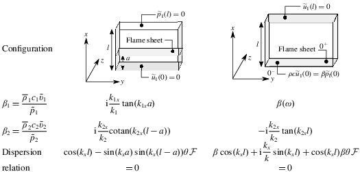
Two different generic configurations represented in table 2 are further investigated. The first one shown on the left is an annular combustor comprising a plenum of height  $a$, which has the same cross-section as the annular combustion chamber and a flame sheet covering the entire annular section. The burnt gases are exhausting in this case at atmospheric pressure. This configuration is a simplified model of the MICCA annular combustor studied at EM2C (Bourgouin et al. Reference Bourgouin, Durox, Moeck, Schuller and Candel2015; Prieur et al. Reference Prieur, Durox, Schuller and Candel2017, Reference Prieur, Durox, Schuller and Candel2018). A more advanced model of the MICCA combustor is presented in § 5.4. In this case the modes are of mixed type meaning that they feature both an axial and azimuthal acoustic components. The right column in table 2 shows an annular combustion chamber terminated by a compact choked nozzle, which is simulated by an acoustic velocity node $\tilde{u} _{1}(l)=0$. This model also takes into account the response of the burners by considering their admittance $\unicode[STIX]{x1D6FD}_{1}=\unicode[STIX]{x1D6FD}$ which remains uniform over the annular cross-section. This type of model often serves in theoretical analysis of the dynamics of purely azimuthal modes corresponding to $\unicode[STIX]{x1D6FD}=0$ (Noiray, Bothien & Schuermans Reference Noiray, Bothien and Schuermans2011; Ghirardo et al. Reference Ghirardo, Juniper and Moeck2016).
Replacing the expressions for  $\unicode[STIX]{x1D6FD}_{1}$ and $\unicode[STIX]{x1D6FD}_{2}$ in table 2 for the two configurations in (3.3) yields the dispersion relations reproduced in the last line in table 2, where it has been further assumed that $\overline{\unicode[STIX]{x1D70C}}_{1}=\overline{\unicode[STIX]{x1D70C}}_{2}=\unicode[STIX]{x1D70C}$ and $c_{1}=c_{2}=c$ to simplify the expressions. In this case, $k_{2x}=k_{1x}=k_{x}$, $k_{2y}=k_{1y}=k_{y}$ and $k_{2}=k_{1}=\unicode[STIX]{x1D714}/c$. Note that this is not a restriction of the method, it is used here to make the expressions more compact.
5.1.1 Instabilities coupled by a mixed azimuthal–longitudinal mode
The dispersion relation associated with the left configuration in table 2 is reproduced here for convenience
 $$\begin{eqnarray}\cos (k_{x}l)-\unicode[STIX]{x1D703}{\mathcal{F}}(\unicode[STIX]{x1D714})\sin (k_{x}a)\sin (k_{x}b)=0,\end{eqnarray}$$
 where  $a+b=l$. Roots of this equation determine the system dynamics and in particular its stability with respect to acoustic perturbations.
In the absence of unsteady flame response  ${\mathcal{F}}=0$, (5.11) reduces to
 $$\begin{eqnarray}{\mathcal{H}}(\unicode[STIX]{x1D714}_{n})=\cos (k_{x}^{n}l)=0\quad \text{i.e. }k_{x}^{n}l=(2n+1)\frac{\unicode[STIX]{x03C0}}{2},\quad n=0,1,2,\ldots .\end{eqnarray}$$
 Inserting these expressions for  $k_{x}^{n}$ in (5.10) fully determines the eigenfrequencies of this annular system
 $$\begin{eqnarray}f_{m}^{n}=c\left[\left(\frac{2n+1}{4l}\right)^{2}+\left(\frac{m+1}{{\mathcal{P}}}\right)^{2}\right]^{1/2},\quad \text{where }n=0,1,2,\ldots \text{ and }m=0,1,2,\ldots .\end{eqnarray}$$
 These expressions confirm that in the absence of flame, the only possible modes are of mixed azimuthal–longitudinal type and are designated as ‘ $(m+1)A-(2n+1)L$’ modes. Purely azimuthal modes are found in the limit of large chamber lengths $l\rightarrow \infty$.
In the following, one considers that the system operates close to the resonant frequencies  $f_{m}^{n}$, which is a combination of the $(2n+1)/4$ wave axial mode of frequency $(2n+1)c/(4l)$ and the $(m+1)$ pure azimuthal mode of frequency $(m+1)c/{\mathcal{P}}$. The frequency of the mixed $(m+1)A-(2n+1)L$ mode in (5.13) is always higher than the frequencies corresponding to the purely $(2n+1)$ axial and purely $(m+1)$ azimuthal modes.
A stability analysis of modes at frequencies  $f_{m}^{n}=\unicode[STIX]{x1D714}_{m}^{n}/(2\unicode[STIX]{x03C0})=k_{m}^{n}/(2\unicode[STIX]{x03C0}c)$ is now carried out by including effects of unsteady heat release. One makes here the same approximation as for the stability analysis of longitudinal modes for which perturbations of the complex angular frequencies were deduced by neglecting the feedback from acoustics on heat release rate disturbances
 $$\begin{eqnarray}\unicode[STIX]{x1D714}_{1}\simeq -\frac{{\mathcal{L}}(\unicode[STIX]{x1D714}_{m}^{n}){\mathcal{F}}(\unicode[STIX]{x1D714}_{m}^{n})}{(\unicode[STIX]{x2202}{\mathcal{H}}/\unicode[STIX]{x2202}\unicode[STIX]{x1D714})_{\unicode[STIX]{x1D714}_{m}^{n}}}.\end{eqnarray}$$
It will be later shown with the EBA approach that this approximation is also pertinent for CIs coupled to azimuthal modes. To do so, one first needs to determine
 $$\begin{eqnarray}\left(\frac{\unicode[STIX]{x2202}{\mathcal{H}}}{\unicode[STIX]{x2202}\unicode[STIX]{x1D714}}\right)_{\unicode[STIX]{x1D714}_{m}^{n}}=\left(\frac{\unicode[STIX]{x2202}{\mathcal{H}}}{\unicode[STIX]{x2202}k_{x}}\right)_{k_{x}^{n}}\left(\frac{\unicode[STIX]{x2202}k_{x}}{\unicode[STIX]{x2202}\unicode[STIX]{x1D714}}\right)_{\unicode[STIX]{x1D714}_{m}^{n}}=\frac{1}{c}\frac{k_{m}^{n}}{k_{x}^{n}}\left(\frac{\unicode[STIX]{x2202}{\mathcal{H}}}{\unicode[STIX]{x2202}k_{x}}\right)_{k_{x}^{n}}.\end{eqnarray}$$
 For  ${\mathcal{H}}(\unicode[STIX]{x1D714})=\cos (k_{x}^{n}l)$, one gets
 $$\begin{eqnarray}\left(\frac{\unicode[STIX]{x2202}{\mathcal{H}}}{\unicode[STIX]{x2202}\unicode[STIX]{x1D714}}\right)_{\unicode[STIX]{x1D714}_{m}^{n}}=-\frac{l}{c}\frac{k_{m}^{n}}{k_{x}^{n}}\sin (k_{m}^{n}l).\end{eqnarray}$$
 For  ${\mathcal{L}}(\unicode[STIX]{x1D714}_{m}^{n})=-\displaystyle \unicode[STIX]{x1D703}\sin (k_{x}^{n}a)\sin (k_{x}^{n}b)$, use of (3.7) leads to the following expression for the complex perturbation in angular frequency $\unicode[STIX]{x1D714}_{1}$ with respect to the modal eigenfrequency $\unicode[STIX]{x1D714}_{m}^{n}$
 $$\begin{eqnarray}\unicode[STIX]{x1D714}_{1}=-\frac{k_{x}^{n}}{k_{m}^{n}}\frac{\sin (k_{x}^{n}a)\sin (k_{x}^{n}b)}{\sin (k_{x}^{n}l)}\frac{c}{l}\unicode[STIX]{x1D703}{\mathcal{F}}(\unicode[STIX]{x1D714}_{m}^{n}).\end{eqnarray}$$
 At resonance  $k_{x}^{n}l=(2n+1)\unicode[STIX]{x03C0}/2$ and $\sin (k_{x}^{n}l)=(-1)^{n}$ and the FTF is represented as ${\mathcal{F}}(\unicode[STIX]{x1D714}_{m}^{n})=G(\unicode[STIX]{x1D714}_{m}^{n})\exp (\text{i}\unicode[STIX]{x1D711}(\unicode[STIX]{x1D714}_{m}^{n}))$. The latter expression reduces to
 $$\begin{eqnarray}\unicode[STIX]{x1D714}_{1}=-(-1)^{n}\frac{k_{x}^{n}}{k_{m}^{n}}\sin \left((2n+1)\frac{\unicode[STIX]{x03C0}a}{2l}\right)\sin \left((2n+1)\frac{\unicode[STIX]{x03C0}b}{2l}\right)\frac{c}{l}\unicode[STIX]{x1D703}G(\unicode[STIX]{x1D714}_{m}^{n})\exp (\text{i}\unicode[STIX]{x1D711}(\unicode[STIX]{x1D714}_{m}^{n})).\end{eqnarray}$$
 The angular frequency disturbance is a complex number  $\unicode[STIX]{x1D714}_{1}=\unicode[STIX]{x0394}\unicode[STIX]{x1D714}_{r}+\text{i}\unicode[STIX]{x1D714}_{i}$, from which one deduces the deviation of the angular frequency $\unicode[STIX]{x0394}\unicode[STIX]{x1D714}_{r}$ with respect to $\unicode[STIX]{x1D714}_{m}^{n}$ and the growth rate $\unicode[STIX]{x1D714}_{i}$ of this perturbation
 $$\begin{eqnarray}\unicode[STIX]{x1D714}_{i}=-(-1)^{n}\frac{k_{x}^{n}}{k_{m}^{n}}\sin \left((2n+1)\frac{\unicode[STIX]{x03C0}a}{2l}\right)\sin \left((2n+1)\frac{\unicode[STIX]{x03C0}b}{2l}\right)\frac{c}{l}\unicode[STIX]{x1D703}G(\unicode[STIX]{x1D714}_{m}^{n})\sin (\unicode[STIX]{x1D711}(\unicode[STIX]{x1D714}_{m}^{n})).\end{eqnarray}$$
 These relations yield the stability bands of all mixed  $(m+1)A-(n+1)L$ azimuthal–longitudinal modes, which are unstable for positive growth rates $\unicode[STIX]{x1D714}_{i}>0$. The first 1A-1L mode is obtained for $m=0$ and $n=0$ at frequency
 $$\begin{eqnarray}f_{0}^{0}=f_{0}=\frac{\unicode[STIX]{x1D714}_{0}}{2\unicode[STIX]{x03C0}}=c\left[\left(\frac{1}{4l}\right)^{2}+\left(\frac{1}{{\mathcal{P}}}\right)^{2}\right]^{1/2}.\end{eqnarray}$$
 The corresponding wavenumber is  $k_{0}^{0}=\unicode[STIX]{x1D714}_{0}/c$ and $k_{x}^{0}l=\unicode[STIX]{x03C0}/2$. This mode is unstable when $\sin (\unicode[STIX]{x1D711}(\unicode[STIX]{x1D714}_{0}))<0$, i.e.
 $$\begin{eqnarray}(2p+1)\unicode[STIX]{x03C0}<\unicode[STIX]{x1D711}(\unicode[STIX]{x1D714}_{0})<2(\,p+1)\unicode[STIX]{x03C0},\quad p=0,1,2,\ldots .\end{eqnarray}$$
 In the unstable bands, one also deduces that when  $(1+2p)\unicode[STIX]{x03C0}<\unicode[STIX]{x1D711}(\unicode[STIX]{x1D714}_{0})<(3/2+2p)\unicode[STIX]{x03C0}$, the instability frequency is slightly higher than the resonant frequency $f_{0}$. When $(3/2+2p)\unicode[STIX]{x03C0}<\unicode[STIX]{x1D711}(\unicode[STIX]{x1D714}_{0})<2(\,p+1)\unicode[STIX]{x03C0}$, the instability frequency is lower than the resonant frequency $f_{0}$.
It is also worth noting that if the flame is located at  $x=a=0$, the system would be unconditionally stable because the axial acoustic velocity normal to the flame front vanishes at this location due to the boundary condition $\tilde{u} _{1}(0)=0$. This problem is revisited in the next section by further considering the role of the response of the injectors in triggering instabilities.
5.1.2 Effects of the burner impedance on a pure 1A azimuthal mode
Close to the chamber backplane, the axial acoustic velocity vanishes and the acoustic field would be mainly oriented in the transverse direction. An unsteady flame sheet transverse to the axial direction would not produce any significant heat release fluctuations in response to this acoustic forcing. Direct effects of the transverse acoustic field were shown to lead to limited high-frequency heat release disturbances (Baillot & Lespinasse Reference Baillot and Lespinasse2013; O’Connor et al. Reference O’Connor, Acharya and Lieuwen2015) that cannot explain the low-frequency and large self-sustained combustion oscillations coupled by azimuthal modes observed in many annular chambers. While the direct effect of transverse fluctuations might alter some of the features of the flow and combustion dynamics in annular systems (Ghirardo & Juniper Reference Ghirardo and Juniper2013; Saurabh, Moeck & Paschereit Reference Saurabh, Moeck and Paschereit2017; Prieur et al. Reference Prieur, Durox, Schuller and Candel2018), a more powerful mechanism is at work.
To limit the pressure drop through the injectors, their response to the pressure oscillation in the annular chamber often induce large perturbations of the mass flow rate through the discharge nozzle (Krebs et al. Reference Krebs, Flohr, Prade and Hoffmann2002; Wolf et al. Reference Wolf, Staffelbach, Gicquel, Muller and Poinsot2012). This mechanism indirectly generates large acoustic velocities normal to the flame front and needs in turn to be considered in the stability analysis. It is shown in the following how to introduce this feature by taking into account the burner impedance.
The analysis is here carried out by considering a velocity node at the combustor exhaust  $\tilde{u} _{2}(l)=0$. This situation prevails when the outlet boundary of the combustor has a high impedance like in gas turbines equipped with choked nozzles. The response of the burners and the plenum to pressure fluctuations in the annular chamber is characterized by an inlet admittance $\unicode[STIX]{x1D6FD}(\unicode[STIX]{x1D714})=\unicode[STIX]{x1D70C}c\tilde{u} _{1}(0)/\tilde{p}_{1}(0)$ (Krebs et al. Reference Krebs, Flohr, Prade and Hoffmann2002). One also further assumes that the flame is located at the chamber backplane by setting $a=0$. This situation corresponds to that shown in the right column in table 2. Only the main steps of the stability analysis are briefly outlined.
The dispersion relation reduces in this case to
 $$\begin{eqnarray}\unicode[STIX]{x1D6FD}\cos (k_{x}l)+\text{i}\frac{k_{x}}{k}\sin (k_{x}l)+\cos (k_{x}l)\unicode[STIX]{x1D703}\unicode[STIX]{x1D6FD}{\mathcal{F}}(\unicode[STIX]{x1D714})=0.\end{eqnarray}$$
Without unsteady heat release, the eigenfrequencies are the solutions of
 $$\begin{eqnarray}{\mathcal{H}}(\unicode[STIX]{x1D714}_{n})=\unicode[STIX]{x1D6FD}\cos (k_{x}^{n}l)+\text{i}\frac{k_{x}^{n}}{k}\sin (k_{x}^{n}l)=0.\end{eqnarray}$$
 The modal structure now explicitly depends on the burner admittance  $\unicode[STIX]{x1D6FD}$. For small admittances $\unicode[STIX]{x1D6FD}\rightarrow 0$, modes correspond to the roots of $\sin (k_{x}^{n}l)=0$. For large admittances $\unicode[STIX]{x1D6FD}\rightarrow \infty$, modes are determined by $\cos (k_{x}^{n}l)=0$. In the general case, it is more difficult to determine explicit expressions of these modes.
It is now convenient to limit the analysis to the first resonant mode of the system  $\unicode[STIX]{x1D714}_{0}$ obtained for $k_{x}^{0}$ and $k_{0}$. At resonance, one has
 $$\begin{eqnarray}\unicode[STIX]{x1D6FD}(\unicode[STIX]{x1D714}_{0})=-\text{i}\frac{k_{x}^{0}}{k_{0}}\tan (k_{x}^{0}l).\end{eqnarray}$$
 By following the same methodology as in the previous section, roots of (5.22) are sought around resonance at  $\unicode[STIX]{x1D714}_{0}$ where ${\mathcal{H}}(\unicode[STIX]{x1D714}_{0})=0$ and the perturbed angular frequency is given by
 $$\begin{eqnarray}\unicode[STIX]{x1D714}_{1}=-\frac{{\mathcal{L}}(\unicode[STIX]{x1D714}_{0}){\mathcal{F}}(\unicode[STIX]{x1D714}_{0})}{\displaystyle \left(\frac{\unicode[STIX]{x2202}{\mathcal{H}}}{\unicode[STIX]{x2202}\unicode[STIX]{x1D714}}\right)_{\unicode[STIX]{x1D714}_{0}}},\end{eqnarray}$$
 with  ${\mathcal{L}}(\unicode[STIX]{x1D714}_{0})=\displaystyle \unicode[STIX]{x1D703}\unicode[STIX]{x1D6FD}(\unicode[STIX]{x1D714}_{0})\cos (k_{x}^{0}l)$ and
 $$\begin{eqnarray}\left(\frac{\unicode[STIX]{x2202}{\mathcal{H}}}{\unicode[STIX]{x2202}\unicode[STIX]{x1D714}}\right)_{\unicode[STIX]{x1D714}_{0}}=\text{i}\frac{l}{c}\cos (k_{x}^{0}l)+\frac{\text{i}}{c}\frac{(k_{y}^{0})^{2}}{k_{x}^{0}k_{0}^{2}}\sin (k_{x}^{0}l)+\text{i}\frac{l}{c}\tan (k_{x}^{0}l)\sin (k_{x}^{0}l),\end{eqnarray}$$
 where  $(k_{x}^{0})^{2}+(k_{y}^{0})^{2}=k_{0}^{2}$ and use has been made of (5.24). It is difficult to get analytical solutions without further simplifications.
In the limit of compact annular chambers  $k_{x}^{0}l\ll 1$, modes are of purely azimuthal type and axial gradients vanish, $k_{x}^{0}\rightarrow 0$ and $k_{y}^{0}=(k_{0}^{2}-(k_{x}^{0})^{1/2})^{1/2}\simeq k_{0}=2\unicode[STIX]{x03C0}/{\mathcal{P}}$. One finds in this limit
 $$\begin{eqnarray}\left(\frac{\unicode[STIX]{x2202}{\mathcal{H}}}{\unicode[STIX]{x2202}\unicode[STIX]{x1D714}}\right)_{\unicode[STIX]{x1D714}_{0}}\simeq \text{i}\frac{l}{c}\left(1+\left(\frac{k_{y}^{0}}{k_{0}}\right)^{2}\right)=\text{i}2\frac{l}{c}\quad \text{and}\quad {\mathcal{L}}(\unicode[STIX]{x1D714}_{0})\simeq \unicode[STIX]{x1D703}\unicode[STIX]{x1D6FD}(\unicode[STIX]{x1D714}_{0}).\end{eqnarray}$$
The perturbed angular frequency is finally given by
 $$\begin{eqnarray}\unicode[STIX]{x1D714}_{1}=\text{i}\frac{1}{2}\frac{c}{l}\unicode[STIX]{x1D703}\unicode[STIX]{x1D6FD}(\unicode[STIX]{x1D714}_{0}){\mathcal{F}}(\unicode[STIX]{x1D714}_{0}).\end{eqnarray}$$
 In this expression, the specific admittance  $\unicode[STIX]{x1D6FD}$ and flame transfer function ${\mathcal{F}}$ are evaluated at the angular frequency $\unicode[STIX]{x1D714}_{0}$. The imaginary component of $\unicode[STIX]{x1D714}_{1}$ yields the perturbation growth rate
 $$\begin{eqnarray}\unicode[STIX]{x1D714}_{i}=\frac{1}{2}\frac{c}{l}\unicode[STIX]{x1D703}\text{Re}[\unicode[STIX]{x1D6FD}(\unicode[STIX]{x1D714}_{0}){\mathcal{F}}(\unicode[STIX]{x1D714}_{0})].\end{eqnarray}$$
 The growth rate of CIs is found to be proportional to  $\unicode[STIX]{x1D703}=T_{2}/T_{1}-1$ and the product of the injector specific admittance $\unicode[STIX]{x1D6FD}$ and flame transfer function ${\mathcal{F}}$ which are both estimated at the resonance angular frequency $\unicode[STIX]{x1D714}_{0}$.
5.2 Energy balance analysis
The objective of the following analysis is to retrieve the growth rates  $\unicode[STIX]{x1D714}_{i}$ for mixed azimuthal-axial modes given by (5.19) and purely azimuthal modes in (5.29) with an alternative method relying on acoustic energy balance calculations. In this approach, there is no approximation regarding the effects of acoustic feedback on heat release disturbances. For this one first calculates the acoustic energy flux originating from the flame. One then obtains the acoustic energy density in the system. Calculations are carried out first for a mixed azimuthal–longitudinal mode and then for a purely azimuthal mode.
The analysis begins by considering the acoustic energy flux flowing through a surface  $S$ characterized by a normal unit vector $\boldsymbol{n}$. This flux integrated over a period of oscillation $T=2\unicode[STIX]{x03C0}/\unicode[STIX]{x1D714}$ is given by $F$ in (2.45). With perturbations expressed in Fourier space, the acoustic energy flux in the normal direction $F$ may also be written as
 $$\begin{eqnarray}F={\textstyle \frac{1}{2}}\text{Re}[\tilde{p}_{1}^{\ast }\tilde{u} _{1}]={\textstyle \frac{1}{2}}\text{Re}[\tilde{p}_{1}\tilde{u} _{1}^{\ast }].\end{eqnarray}$$
Across the flame sheet, the acoustic pressure being constant (2.8) and the velocity jump being given by (2.14), their products also write
 $$\begin{eqnarray}\tilde{p}_{2}^{\ast }\tilde{u} _{2}=\tilde{p}_{1}^{\ast }\tilde{u} _{1}(1+\unicode[STIX]{x1D703}\,{\mathcal{F}}(\unicode[STIX]{x1D714})).\end{eqnarray}$$
Taking the real component of this expression leads to
 $$\begin{eqnarray}F_{2}-F_{1}=\unicode[STIX]{x1D703}\,\text{Re}[Y_{1}{\mathcal{F}}(\unicode[STIX]{x1D714})]{\textstyle \frac{1}{2}}|\tilde{p}_{1}|^{2},\end{eqnarray}$$
 where  $Y_{1}=\tilde{u} _{1}/\tilde{p}_{1}=\bar{\unicode[STIX]{x1D70C}}_{1}c_{1}\unicode[STIX]{x1D6FD}_{1}$ denotes the injector admittance. It is worth noting that the acoustic flux $F_{1}$ through the injector may also be expressed as a function of the injector admittance $F_{1}=\text{Re}[Y_{1}](1/2)|\tilde{p}_{1}|^{2}$.
Integration of (5.32) over the cross-section area  $S$ of the flame yields an expression for the supplementary acoustic energy flux resulting from the flame response to acoustic perturbations that delivers unsteady perturbations in heat release rate
 $$\begin{eqnarray}{\mathcal{R}}=\int _{S}(F_{2}-F_{1})\,\text{d}S=\int _{S}\unicode[STIX]{x1D703}\,\text{Re}[Y_{1}{\mathcal{F}}(\unicode[STIX]{x1D714})]\frac{1}{2}|\tilde{p}_{1}|^{2}\,\text{d}S.\end{eqnarray}$$
 This expression yields an alternative form of the Rayleigh index  ${\mathcal{R}}$ appearing in the acoustic energy balance (2.43) and highlights the main parameters controlling the susceptibility of the system to combustion instabilities. The excess of acoustic power is proportional to $\unicode[STIX]{x1D703}=T_{2}/T_{1}-1$. It is also proportional to the real component of the product of the injector admittance $Y_{1}$ and FTF ${\mathcal{F}}$. This latter contribution is intrinsic to the flame/injector system describing its frequency response to acoustic perturbations.
The growth rate of oscillations can then be deduced by taking the ratio of the power flow into the system due to the flame to the total acoustic energy in the combustor volume  $V$ (Cantrell & Hart Reference Cantrell and Hart1964) as explained in the tutorial section
 $$\begin{eqnarray}2\unicode[STIX]{x1D714}_{i}=\frac{{\mathcal{R}}-{\mathcal{D}}}{{\mathcal{E}}}=\left.\int _{S}(F_{2}-F_{1})\,\text{d}S\right/\int _{V}E\,\text{d}V,\end{eqnarray}$$
 where  ${\mathcal{D}}=0$ because $\tilde{p}$ or $\tilde{u}$ are zero at the system boundaries in the selected examples and $\unicode[STIX]{x1D714}_{i}=\text{Im}(\unicode[STIX]{x1D714})$ is the imaginary component of the angular frequency.
A ‘stiff’ injector is defined by an infinite impedance or a vanishing admittance  $Y_{1}\simeq 0$ corresponding to a vanishing velocity perturbation $\tilde{u} _{1}\simeq 0$. Increasing the acoustic stiffness of the air injector is a way to reduce the system susceptibility to CIs, but this is generally accompanied by an increase of the pressure drop. In many practical systems, the pressure drop through the air injection units needs to be minimized leading to designs with a relatively low impedance featuring a ‘loose’ injector response to acoustic perturbations. For a pressure release air injector, $\tilde{p}_{1}\simeq 0$ and $Y_{1}\rightarrow \infty$, the excess of acoustic flux is in this case solely determined by the FTF ${\mathcal{F}}$. The role of the injector specific admittance $\unicode[STIX]{x1D6FD}$ for CIs coupled to azimuthal modes is further discussed in § 5.4.
5.2.1 Energy balance analysis for mixed azimuthal–longitudinal modes
Calculations are first carried out for the configuration shown on the left in table 2 featuring a rigid wall on the upstream side  $x=0$ and an open boundary at the outlet $x=l$ with a flame sheet at $x=0$. They make use of results from the previous section and in particular those obtained by considering that the oscillation is close to a resonant mode of the system. Due to the pressure release outlet, modes are of mixed azimuthal–longitudinal types.
The pressure and axial velocity just upstream of the flame are as follows
 $$\begin{eqnarray}\tilde{p}_{1}=A\cos (k_{x}x)\unicode[STIX]{x1D713}(\,y)\quad \text{and}\quad \bar{\unicode[STIX]{x1D70C}}c\tilde{u} _{1}=\text{i}A\frac{k_{x}}{k}\sin (k_{x}x)\unicode[STIX]{x1D713}(\,y),\end{eqnarray}$$
 where  $A$ is a constant and $\unicode[STIX]{x1D713}(\,y)=\cos (k_{y}^{m}y)$ or $\sin (k_{y}^{m}y)$ or a linear combination of these two functions. The specific admittance upstream of the flame is in this case
 $$\begin{eqnarray}\unicode[STIX]{x1D6FD}=\text{i}\frac{k_{x}}{k}\frac{\sin (k_{x}a)}{\cos (k_{x}a)},\end{eqnarray}$$
 where  $k=(k_{x}^{2}+k_{y}^{2})^{1/2}=\unicode[STIX]{x1D714}/c$. The admittance is purely imaginary and as a consequence the acoustic energy flux $F_{1}$ on the upstream side of the flame is zero $F_{1}=0$. Expression (5.32) yields the acoustic flux downstream the flame
 $$\begin{eqnarray}F_{2}=-\unicode[STIX]{x1D703}\frac{1}{2\bar{\unicode[STIX]{x1D70C}}c}|\tilde{p}_{1}|^{2}\frac{k_{x}}{k}\frac{\sin (k_{x}a)}{\cos (k_{x}a)}G(\unicode[STIX]{x1D714})\sin [\unicode[STIX]{x1D711}(\unicode[STIX]{x1D714})].\end{eqnarray}$$
This flux is positive if
 $$\begin{eqnarray}\frac{\sin (k_{x}a)}{\cos (k_{x}a)}\sin [\unicode[STIX]{x1D711}(\unicode[STIX]{x1D714})]<0.\end{eqnarray}$$
 Considering for example the 1A-1L mode for which  $k_{x}^{0}=\unicode[STIX]{x03C0}/(2l)$ so that both $\sin (k_{x}^{0}a)$ and $\cos (k_{x}^{0}a)$ are positive, the condition for instability is $\unicode[STIX]{x03C0}<\unicode[STIX]{x1D711}<2\unicode[STIX]{x03C0}$, modulo $2\unicode[STIX]{x03C0}$. When this condition is satisfied the power flow from the flame region is positive and it was seen previously that this condition on the phase lag $\unicode[STIX]{x1D711}$ of the FTF was also necessary to obtain an instability coupled by the 1A-1L mode of the chamber.
It is convenient to rewrite the energy flux  $F_{2}$ in (5.37) by making use of the pressure field expression calculated in the section $x=a$ and noting that
 $$\begin{eqnarray}|\tilde{p}_{1}(x=a)|^{2}=|A|^{2}\cos ^{2}(k_{x}a)|\unicode[STIX]{x1D713}(\,y)|^{2}.\end{eqnarray}$$
Inserting this expression in (5.37) leads to
 $$\begin{eqnarray}F_{2}=-\unicode[STIX]{x1D703}G(\unicode[STIX]{x1D714})\frac{1}{2\bar{\unicode[STIX]{x1D70C}}c}|A|^{2}\frac{k_{x}}{k}\sin (k_{x}a)\cos (k_{x}a)\sin [\unicode[STIX]{x1D711}(\unicode[STIX]{x1D714})]|\unicode[STIX]{x1D713}(\,y)|^{2}.\end{eqnarray}$$
 One may now assume that the pressure field corresponds to a resonance of the system such that  $\cos (k_{x}^{n}l)=0$. This yields discrete values of the axial wavenumber $k_{x}^{n}=(2n+1)\unicode[STIX]{x03C0}/(2l)$, where $n=0,1,2,\ldots .$ It is also easy to show that $\cos (k_{x}^{n}a)=(-1)^{n}\sin (k_{x}^{n}b)$ where $b=l-a$ and the acoustic energy flux becomes
 $$\begin{eqnarray}F_{2}=-(-1)^{n}\unicode[STIX]{x1D703}G(\unicode[STIX]{x1D714})\frac{1}{2\unicode[STIX]{x1D70C}_{0}c}|A|^{2}\frac{k_{x}^{n}}{k_{n}}\sin (k_{x}^{n}a)\sin (k_{x}^{n}b)\sin [\unicode[STIX]{x1D711}(\unicode[STIX]{x1D714})]|\unicode[STIX]{x1D713}(\,y)|^{2}.\end{eqnarray}$$
One may now calculate the energy density in the system integrated over an oscillation period of the mode
 $$\begin{eqnarray}E=\frac{1}{2}\left[\frac{1}{2}\frac{|\tilde{p}_{1}|^{2}}{\bar{\unicode[STIX]{x1D70C}}c^{2}}+\frac{1}{2}\bar{\unicode[STIX]{x1D70C}}|\tilde{u} _{1}|^{2}+\frac{1}{2}\bar{\unicode[STIX]{x1D70C}}|\tilde{v}_{1}|^{2}\right].\end{eqnarray}$$
 It is important to include in this expression the kinetic energy corresponding to the longitudinal and transverse velocity components. This quantity has to be integrated in the longitudinal and transverse directions and over the thickness  $d$ of the system corresponding to the distance between the inner and outer walls of the combustor. One finds after some algebra that the integrated value of the last two terms (corresponding to kinetic energy) is equal to the integrated value of the first term (corresponding to elastic energy)
 $$\begin{eqnarray}\int _{V}\left[\frac{1}{2}\bar{\unicode[STIX]{x1D70C}}|\tilde{u} _{1}|^{2}+\frac{1}{2}\bar{\unicode[STIX]{x1D70C}}|\tilde{v}_{1}|^{2}\right]\text{d}V=\int _{V}\frac{1}{2}\frac{|\tilde{p}_{1}|^{2}}{\bar{\unicode[STIX]{x1D70C}}c^{2}}\text{d}V,\end{eqnarray}$$
and one obtains
 $$\begin{eqnarray}\int _{V}\frac{1}{2}\frac{|\tilde{p}_{1}|^{2}}{\bar{\unicode[STIX]{x1D70C}}c^{2}}\text{d}V=\frac{1}{2}\frac{|A|^{2}}{\bar{\unicode[STIX]{x1D70C}}c^{2}}\frac{l{\mathcal{P}}d}{4},\end{eqnarray}$$
 where  ${\mathcal{P}}$ denotes the perimeter of the midline circle crossing the centre of each burner in the annular chamber. This finally leads to
 $$\begin{eqnarray}\int _{V}E\,\text{d}V=\frac{|A|^{2}}{\bar{\unicode[STIX]{x1D70C}}c^{2}}\frac{l{\mathcal{P}}d}{8}.\end{eqnarray}$$
 It is then necessary to integrate the acoustic fluxes  $F_{1}$ and $F_{2}$ over the surface $S$. It was already indicated that $F_{1}=0$ and one obtains
 $$\begin{eqnarray}\int _{S}F_{2}\,\text{d}S=-(-1)^{n}\unicode[STIX]{x1D703}G(\unicode[STIX]{x1D714})\frac{1}{2\bar{\unicode[STIX]{x1D70C}}c}|A|^{2}\frac{k_{x}^{n}}{k_{n}}\sin (k_{x}^{n}a)\sin (k_{x}^{n}b)\sin [\unicode[STIX]{x1D711}(\unicode[STIX]{x1D714})]\frac{{\mathcal{P}}d}{2}.\end{eqnarray}$$
The last two expressions inserted in (5.34) yield the growth rate of perturbations
 $$\begin{eqnarray}\unicode[STIX]{x1D714}_{i}=-(-1)^{n}\frac{k_{x}^{n}}{k_{n}}\sin (k_{x}^{n}a)\sin (k_{x}^{n}b)\frac{c}{l}\unicode[STIX]{x1D703}G(\unicode[STIX]{x1D714})\sin [\unicode[STIX]{x1D711}(\unicode[STIX]{x1D714})].\end{eqnarray}$$
This exactly coincides with the expression (5.19) obtained previously for the growth rate of instabilities coupled to a mixed azimuthal–longitudinal mode under the assumption that the presence of the flame and its transfer function only weakly perturb the wave field in the system. This energy balance approach validates the approximation adopted in determining the growth rates of CIs with (3.7).
5.2.2 Instabilities coupled by a purely azimuthal mode
It is next interesting to examine the stability of a purely azimuthal mode with the energy method exploited previously. The geometry considered is that in the right column in table 2 with a flame sheet lying at the bottom of the combustion chamber at  $x=a=0$. In this case, modes are uniform in the axial direction and have the form
 $$\begin{eqnarray}\unicode[STIX]{x1D713}(\,y)\exp (-\text{i}\unicode[STIX]{x1D714}t),\end{eqnarray}$$
 where  $\unicode[STIX]{x1D713}(\,y)$ is equal to $\cos (k_{y}y)$ or $\sin (k_{y}y)$ or consists of a linear combination of these two functions. The wavenumber $k$ reduces in this case to $k=k_{y}=\unicode[STIX]{x1D714}/c$. The periodicity condition (5.2) yields the modal angular frequencies $k_{y}^{m}=(m+1)2\unicode[STIX]{x03C0}/{\mathcal{P}}=\unicode[STIX]{x1D714}_{m}/c$, with $m=0,1,2,\ldots .$ And the structure of the corresponding pressure and velocity fields is then given by
 $$\begin{eqnarray}\displaystyle & \displaystyle \tilde{p}_{1}=A\unicode[STIX]{x1D713}(\,y), & \displaystyle\end{eqnarray}$$
 $$\begin{eqnarray}\displaystyle & \displaystyle \overline{\unicode[STIX]{x1D70C}}c\tilde{u} _{1}=0, & \displaystyle\end{eqnarray}$$
 $$\begin{eqnarray}\displaystyle & \displaystyle \overline{\unicode[STIX]{x1D70C}}c\tilde{v}_{1}=-\text{i}A\unicode[STIX]{x1D713}^{\prime }(\,y), & \displaystyle\end{eqnarray}$$
 where  $\unicode[STIX]{x1D713}^{\prime }(\,y)=-\text{sin}(k_{y}^{m}y)$ if $\unicode[STIX]{x1D713}(\,y)=\cos (k_{y}^{m}y)$ and $\unicode[STIX]{x1D713}^{\prime }(\,y)=\cos (k_{y}^{m}y)$ if $\unicode[STIX]{x1D713}(\,y)=\sin (k_{y}^{m}y)$. It is worth noting that in this case, there is so far no axial acoustic velocity acting on the flame sheet.
As a consequence, the acoustic flux in the normal direction on the upstream side of the flame corresponding to this purely azimuthal mode vanishes. However, if one assumes that on the upstream side of the flame, the pressure field acts on the injector outlet producing a normal velocity  $\tilde{u} _{1}$, this will produce an incoming acoustic flux. Assuming the injector may be represented by its specific admittance $\unicode[STIX]{x1D6FD}$, the incoming acoustic energy flux writes
 $$\begin{eqnarray}F_{1}=\frac{1}{2}\frac{\text{Re}[\unicode[STIX]{x1D6FD}]}{\bar{\unicode[STIX]{x1D70C}}c}|\tilde{p}_{1}|^{2}=\frac{1}{2}\frac{|A|^{2}}{\overline{\unicode[STIX]{x1D70C}}c}\text{Re}[\unicode[STIX]{x1D6FD}]|\unicode[STIX]{x1D713}(\,y)|^{2}.\end{eqnarray}$$
One may now use (5.32) in which the pressure field is replaced by (5.49) to get
 $$\begin{eqnarray}F_{2}-F_{1}=\unicode[STIX]{x1D703}\text{Re}[{\mathcal{F}}(\unicode[STIX]{x1D714}_{n})\unicode[STIX]{x1D6FD}]\frac{1}{2}\frac{|A|^{2}}{\overline{\unicode[STIX]{x1D70C}}c}|\unicode[STIX]{x1D713}(\,y)|^{2}.\end{eqnarray}$$
 It is now easy to calculate the integral of the fluxes over the surface  $S$
$S$
 $$\begin{eqnarray}\int _{S}(F_{2}-F_{1})\,\text{d}S=\unicode[STIX]{x1D703}\text{Re}[{\mathcal{F}}(\unicode[STIX]{x1D714}_{n})\unicode[STIX]{x1D6FD}]\frac{1}{2}\frac{|A|^{2}}{\overline{\unicode[STIX]{x1D70C}}c}\frac{{\mathcal{P}}d}{2}.\end{eqnarray}$$
The next step is to determine the acoustic energy density and integrate this density over the combustor volume. The energy density now only comprises two terms, the first corresponds to the elastic energy associated with the pressure while the second is the kinetic energy pertaining to the velocity in the transverse direction
 $$\begin{eqnarray}E=\frac{1}{2}\left[\frac{1}{2}\frac{|\tilde{p}_{1}|^{2}}{\bar{\unicode[STIX]{x1D70C}}c^{2}}+\frac{1}{2}\bar{\unicode[STIX]{x1D70C}}|\tilde{v}_{1}|^{2}\right].\end{eqnarray}$$
One may again show that when these two terms are integrated over the volume they yield equal contributions and that
 $$\begin{eqnarray}\int _{V}E\,\text{d}V=\frac{l{\mathcal{P}}d}{4}\frac{|A|^{2}}{\overline{\unicode[STIX]{x1D70C}}c^{2}}.\end{eqnarray}$$
One deduces the following expression for the growth rate by making use of (5.34)
 $$\begin{eqnarray}\unicode[STIX]{x1D714}_{i}=\frac{1}{2}\frac{c}{l}\unicode[STIX]{x1D703}\,\text{Re}[\unicode[STIX]{x1D6FD}(\unicode[STIX]{x1D714}_{n}){\mathcal{F}}(\unicode[STIX]{x1D714}_{n})].\end{eqnarray}$$
 Again this expression for the growth rate corresponds to (5.29) obtained with the CFDM for an instability coupled to a purely azimuthal mode. Note that it does not depend on the axial position of the flame but is a function of the injector response through its specific admittance  $\unicode[STIX]{x1D6FD}$. This expression also differs from that obtained from a mixed azimuthal–longitudinal mode by a factor of 2 which comes from the fact that the acoustic energy in this mode is twice that of the modes featuring an axial structure.
It is interesting to express the injector admittance as  $\unicode[STIX]{x1D6FD}=B(\unicode[STIX]{x1D714}_{n})\exp (\text{i}\unicode[STIX]{x03C0}+\text{i}\unicode[STIX]{x1D6FF})$ and to use ${\mathcal{F}}(\unicode[STIX]{x1D714}_{n})=G(\unicode[STIX]{x1D714}_{n})\exp (\text{i}\unicode[STIX]{x1D711})$ leading to
 $$\begin{eqnarray}\unicode[STIX]{x1D714}_{i}=-\frac{1}{2}\unicode[STIX]{x1D703}\,\frac{c}{l}\,G(\unicode[STIX]{x1D714}_{n})B(\unicode[STIX]{x1D714}_{n})\cos (\unicode[STIX]{x1D711}+\unicode[STIX]{x1D6FF}),\end{eqnarray}$$
 which shows that growth rate of CIs are positive if the phase  $\unicode[STIX]{x1D711}$ belongs to the interval $[\unicode[STIX]{x03C0}/2-\unicode[STIX]{x1D6FF},3\unicode[STIX]{x03C0}/2-\unicode[STIX]{x1D6FF}],\;\text{modulo}\;2\unicode[STIX]{x03C0}$.
5.3 Discrete flame source model
A third way to analyse azimuthal instabilities is now explored. In this model, designated as DFSM, one considers a set of discrete unsteady combustion sources periodically distributed in the annular system and one assumes that these combustion regions may be assimilated to point sources as in figure 22(b). The sound field is then obtained by making use of a modal expansion of the pressure (Culick Reference Culick2001). This is then used to derive a dispersion relation and perform a stability analysis.
One begins with a reactive flow wave equation that may be cast in the form (Crighton et al. Reference Crighton, Dowling, Ffowcs Williams, Heckl and Leppington1992)
 $$\begin{eqnarray}\frac{\unicode[STIX]{x2202}^{2}p^{\prime }}{\unicode[STIX]{x2202}t^{2}}+2\unicode[STIX]{x1D6FC}\frac{\unicode[STIX]{x2202}p^{\prime }}{\unicode[STIX]{x2202}t}-\overline{\unicode[STIX]{x1D70C}}c^{2}\unicode[STIX]{x1D735}\boldsymbol{\cdot }\left(\frac{1}{\overline{\unicode[STIX]{x1D70C}}}\unicode[STIX]{x1D735}p^{\prime }\right)=(\unicode[STIX]{x1D6FE}-1)\frac{\unicode[STIX]{x2202}\dot{q}^{\prime }}{\unicode[STIX]{x2202}t}.\end{eqnarray}$$
 This equation includes a damping term with a damping rate  $\unicode[STIX]{x1D6FC}$. On the right-hand side is the volumetric unsteady heat release rate term which constitutes a source of the wave field.
It is convenient to use the normal modes of a wave equation without the damping term ( $\unicode[STIX]{x1D6FC}=0$) and without the unsteady flame ( $\dot{q}^{\prime }=0$). These modes are solutions of
 $$\begin{eqnarray}\overline{\unicode[STIX]{x1D70C}}c^{2}\unicode[STIX]{x1D735}\boldsymbol{\cdot }\left(\frac{1}{\overline{\unicode[STIX]{x1D70C}}}\unicode[STIX]{x1D735}\unicode[STIX]{x1D713}_{n}\right)+\unicode[STIX]{x1D714}_{n}^{2}\unicode[STIX]{x1D713}_{n}=0.\end{eqnarray}$$
These normal modes are orthogonal if the boundary conditions imposed to the pressure field are of the Dirichlet, Von Neumann or mixed type. We assume that this is the case so that
 $$\begin{eqnarray}\int _{V}\unicode[STIX]{x1D713}_{n}\unicode[STIX]{x1D713}_{m}\,\text{d}V=\unicode[STIX]{x1D6EC}_{n}\unicode[STIX]{x1D6FF}_{mn}.\end{eqnarray}$$
 In this expression  $\unicode[STIX]{x1D6EC}_{n}$ represents the energy of the $n$th mode and $\unicode[STIX]{x1D6FF}_{mn}=0$ when $m\neq n$ and $\unicode[STIX]{x1D6FF}_{mn}=1$ when $m=n$. The pressure field is now expanded as
 $$\begin{eqnarray}p^{\prime }(\boldsymbol{x},t)=\mathop{\sum }_{n}\unicode[STIX]{x1D702}_{n}(t)\unicode[STIX]{x1D713}_{n}(\boldsymbol{x}),\end{eqnarray}$$
 where  $\unicode[STIX]{x1D702}_{n}(t)$ are the amplitudes of this modal expansion. Inserting this expression in the wave equation and projecting on one of the modes, one obtains a set of differential equations for the modal amplitudes
 $$\begin{eqnarray}\frac{\text{d}^{2}\unicode[STIX]{x1D702}_{n}}{\text{d}t^{2}}+2\unicode[STIX]{x1D6FC}\frac{\text{d}\unicode[STIX]{x1D702}_{n}}{\text{d}t}+\unicode[STIX]{x1D714}_{n}^{2}\unicode[STIX]{x1D702}_{n}=\frac{1}{\unicode[STIX]{x1D6EC}_{n}}(\unicode[STIX]{x1D6FE}-1)\int _{V}\frac{\unicode[STIX]{x2202}\dot{q}^{\prime }}{\unicode[STIX]{x2202}t}\unicode[STIX]{x1D713}_{n}\,\text{d}V.\end{eqnarray}$$
 To pursue this analysis one has to specify the unsteady heat release source terms. One considers that there are  $N$ injection points periodically distributed in the annular combustor. It is also assumed that each flame acts like a point source
 $$\begin{eqnarray}\dot{q}^{\prime }=\mathop{\sum }_{j=0}^{N-1}\dot{Q}_{j}^{\prime }\unicode[STIX]{x1D6FF}(\boldsymbol{x}-\boldsymbol{x}_{j}).\end{eqnarray}$$
The right-hand side of (5.63) becomes
 $$\begin{eqnarray}J=\frac{1}{\unicode[STIX]{x1D6EC}_{n}}(\unicode[STIX]{x1D6FE}-1)\int _{V}\frac{\unicode[STIX]{x2202}\dot{q}^{\prime }}{\unicode[STIX]{x2202}t}\unicode[STIX]{x1D713}_{n}\,\text{d}V=\frac{1}{\unicode[STIX]{x1D6EC}_{n}}(\unicode[STIX]{x1D6FE}-1)\mathop{\sum }_{j=0}^{N-1}\frac{\text{d}\dot{Q}_{j}^{\prime }}{\text{d}t}\unicode[STIX]{x1D713}_{n}(\boldsymbol{x}_{j}),\end{eqnarray}$$
and the amplitude equations become
 $$\begin{eqnarray}\frac{\text{d}^{2}\unicode[STIX]{x1D702}_{n}}{\text{d}t^{2}}+2\unicode[STIX]{x1D6FC}\frac{\text{d}\unicode[STIX]{x1D702}_{n}}{\text{d}t}+\unicode[STIX]{x1D714}_{n}^{2}\unicode[STIX]{x1D702}_{n}=\frac{1}{\unicode[STIX]{x1D6EC}_{n}}(\unicode[STIX]{x1D6FE}-1)\mathop{\sum }_{j=0}^{N-1}\frac{\text{d}\dot{Q}_{j}^{\prime }}{\text{d}t}\unicode[STIX]{x1D713}_{n}(\boldsymbol{x}_{j}).\end{eqnarray}$$
These equations may now be written in the frequency domain
 $$\begin{eqnarray}(-\unicode[STIX]{x1D714}^{2}-2\text{i}\unicode[STIX]{x1D6FC}\unicode[STIX]{x1D714}+\unicode[STIX]{x1D714}_{n}^{2})\widetilde{\unicode[STIX]{x1D702}}_{n}=(-\text{i}\unicode[STIX]{x1D714})\frac{1}{\unicode[STIX]{x1D6EC}_{n}}(\unicode[STIX]{x1D6FE}-1)\mathop{\sum }_{j=0}^{N-1}\widetilde{\dot{Q}}_{j}\unicode[STIX]{x1D713}_{n}(\boldsymbol{x}_{j}).\end{eqnarray}$$
The unsteady heat release rate is expressed by making use of the FTF
 $$\begin{eqnarray}\widetilde{\dot{Q}}_{j}=\overline{\dot{Q}}_{j}\,{\mathcal{F}}(\unicode[STIX]{x1D714})\frac{\tilde{u} _{j}}{\overline{u}}.\end{eqnarray}$$
 Next, it is reasonable to assume that the mean heat release rate is the same for all flames and write  $\overline{\dot{Q}}_{j}=\overline{\dot{Q}}_{0}$. The velocity perturbation at the $j$th injection point may be expressed in terms of the pressure at that point by making use of the injector impedance
 $$\begin{eqnarray}\tilde{u} _{j}=\frac{\tilde{p}_{j}}{Z(\unicode[STIX]{x1D714})}=\frac{1}{Z(\unicode[STIX]{x1D714})}\mathop{\sum }_{m}\tilde{\unicode[STIX]{x1D702}}_{m}\unicode[STIX]{x1D713}_{m}(\boldsymbol{x}_{j}).\end{eqnarray}$$
The amplitude equations in frequency space become
 $$\begin{eqnarray}(\unicode[STIX]{x1D714}^{2}+2\text{i}\unicode[STIX]{x1D6FC}\unicode[STIX]{x1D714}-\unicode[STIX]{x1D714}_{n}^{2})\widetilde{\unicode[STIX]{x1D702}}_{n}=(\text{i}\unicode[STIX]{x1D714})\frac{1}{\unicode[STIX]{x1D6EC}_{n}}(\unicode[STIX]{x1D6FE}-1)\frac{\overline{\dot{Q}}_{0}}{\overline{u}}\frac{{\mathcal{F}}(\unicode[STIX]{x1D714})}{Z(\unicode[STIX]{x1D714})}\mathop{\sum }_{j=0}^{N-1}\mathop{\sum }_{m}\tilde{\unicode[STIX]{x1D702}}_{m}\unicode[STIX]{x1D713}_{n}(\boldsymbol{x}_{j})\unicode[STIX]{x1D713}_{m}(\boldsymbol{x}_{j}).\end{eqnarray}$$
 At this point it is worth considering the modal eigenfunctions  $\unicode[STIX]{x1D713}_{n}(\boldsymbol{x}_{j})$. In some general configurations, it is possible to write these modal functions as a product of a function corresponding to the transverse structure and another function describing the axial distribution
 $$\begin{eqnarray}\unicode[STIX]{x1D713}_{n}(\boldsymbol{x}_{j})=\unicode[STIX]{x1D713}_{\bot n}(\boldsymbol{x}_{\bot j})\unicode[STIX]{x1D713}_{\Vert n}(x_{j}),\end{eqnarray}$$
 where  $\boldsymbol{x}_{\bot j}$ and $x_{j}$ respectively designate the transverse and axial positions. One may now assume that the sources corresponding to all flames are located at the same axial position $x_{j}=a$. This allows a considerable simplification of the double sum appearing in (5.70):
 $$\begin{eqnarray}\mathop{\sum }_{j=0}^{N-1}\mathop{\sum }_{m}\tilde{\unicode[STIX]{x1D702}}_{m}\unicode[STIX]{x1D713}_{n}(\boldsymbol{x}_{j})\unicode[STIX]{x1D713}_{m}(\boldsymbol{x}_{j})=\mathop{\sum }_{m}\tilde{\unicode[STIX]{x1D702}}_{m}\unicode[STIX]{x1D713}_{\Vert n}(a)\unicode[STIX]{x1D713}_{\Vert m}(a)\mathop{\sum }_{j=0}^{N-1}\unicode[STIX]{x1D713}_{\bot n}(\boldsymbol{x}_{\bot j})\unicode[STIX]{x1D713}_{\bot m}(\boldsymbol{x}_{\bot j}).\end{eqnarray}$$
 In the annular case situation one may consider that the transverse position corresponds to a single coordinate  $y_{j}$ so that $\unicode[STIX]{x1D713}_{\bot n}(\boldsymbol{x}_{\bot j})=\unicode[STIX]{x1D713}_{\bot n}(\,y_{j})$, and the last sum can be calculated approximately as an integral by multiplying this sum by $\unicode[STIX]{x0394}y={\mathcal{P}}/N$
 $$\begin{eqnarray}I=\mathop{\sum }_{j=0}^{N-1}\unicode[STIX]{x1D713}_{\bot n}(\boldsymbol{x}_{\bot j})\unicode[STIX]{x1D713}_{\bot m}(\boldsymbol{x}_{\bot j})=\frac{1}{\unicode[STIX]{x0394}y}\mathop{\sum }_{j=0}^{N-1}\unicode[STIX]{x1D713}_{\bot n}(\,y_{j})\unicode[STIX]{x1D713}_{\bot m}(\,y_{j})\unicode[STIX]{x0394}y,\end{eqnarray}$$
 which has the form of a Riemann sum. When  $\unicode[STIX]{x0394}y$ is sufficiently small this sum is approximately equal to an integral:
 $$\begin{eqnarray}I\simeq \frac{1}{\unicode[STIX]{x0394}y}\int _{0}^{{\mathcal{P}}}\unicode[STIX]{x1D713}_{\bot n}(\,y)\unicode[STIX]{x1D713}_{\bot m}(\,y)\,\text{d}y.\end{eqnarray}$$
 Considering a typical expression of the transverse modal structure  $\unicode[STIX]{x1D713}_{\bot n}(\,y)=\cos (k_{y}^{n}y)$ or $\sin (k_{y}^{n}y)$ one finds that
 $$\begin{eqnarray}\int _{0}^{{\mathcal{P}}}\unicode[STIX]{x1D713}_{\bot n}(\,y)\unicode[STIX]{x1D713}_{\bot m}(\,y)\,\text{d}y=\frac{{\mathcal{P}}}{2}\unicode[STIX]{x1D6FF}_{mn},\end{eqnarray}$$
leading to
 $$\begin{eqnarray}I=\frac{N}{2}\unicode[STIX]{x1D6FF}_{mn}.\end{eqnarray}$$
The right-hand side of equation (5.70) becomes
 $$\begin{eqnarray}(\text{i}\unicode[STIX]{x1D714})\frac{1}{\unicode[STIX]{x1D6EC}_{n}}(\unicode[STIX]{x1D6FE}-1)\frac{\overline{\dot{Q}}_{0}}{\overline{u}}\frac{{\mathcal{F}}(\unicode[STIX]{x1D714})}{Z(\unicode[STIX]{x1D714})}\frac{N}{2}[\unicode[STIX]{x1D713}_{\Vert n}(a)]^{2}\,\tilde{\unicode[STIX]{x1D702}}_{n}.\end{eqnarray}$$
 It is now convenient to use the specific admittance and write  $Z=\overline{\unicode[STIX]{x1D70C}}c/\unicode[STIX]{x1D6FD}$, noting that $\overline{\dot{Q}}=N\overline{\dot{Q}_{0}}$ and multiplying by $\unicode[STIX]{x1D6FE}\overline{p}=\overline{\unicode[STIX]{x1D70C}}c^{2}$. One also has to take into account that $\unicode[STIX]{x1D6EC}_{n}={\mathcal{P}}\,\text{d}l/4$ for mixed azimuthal–longitudinal modes and $\unicode[STIX]{x1D6EC}_{n}={\mathcal{P}}\,\text{d}l/2$ for purely azimuthal modes. One then obtains for the right-hand side of (5.70)
 $$\begin{eqnarray}2^{s}\,(\text{i}\unicode[STIX]{x1D714})\frac{\unicode[STIX]{x1D6FE}-1}{\unicode[STIX]{x1D6FE}}\frac{\overline{\dot{Q}}}{\overline{p}S\,\overline{u}}\,\frac{c}{l}\,{\mathcal{F}}(\unicode[STIX]{x1D714})\unicode[STIX]{x1D6FD}(\unicode[STIX]{x1D714})[\unicode[STIX]{x1D713}_{\Vert n}(a)]^{2s}\,\tilde{\unicode[STIX]{x1D702}}_{n},\end{eqnarray}$$
 where  $s=0$ for purely azimuthal modes and $s=1$ for mixed azimuthal–longitudinal modes. This expression features the factor $\unicode[STIX]{x1D703}=[(\unicode[STIX]{x1D6FE}-1)/\unicode[STIX]{x1D6FE}]\overline{\dot{Q}}/(\,\overline{p}S\,\overline{u})=T_{2}/T_{1}-1$ already exhibited in the preceding analysis. Inserting this latter expression in (5.70) one obtains the following dispersion relation:
 $$\begin{eqnarray}\unicode[STIX]{x1D714}^{2}+2\text{i}\unicode[STIX]{x1D6FC}\unicode[STIX]{x1D714}-\unicode[STIX]{x1D714}_{n}^{2}=2^{s}\,(\text{i}\unicode[STIX]{x1D714})\unicode[STIX]{x1D703}\,\frac{c}{l}\,{\mathcal{F}}(\unicode[STIX]{x1D714})\unicode[STIX]{x1D6FD}(\unicode[STIX]{x1D714})[\unicode[STIX]{x1D713}_{\Vert n}(a)]^{2s}.\end{eqnarray}$$
 This expression can be used to determine the roots  $\unicode[STIX]{x1D714}$ corresponding to each of the perturbed modes of the system. If the imaginary part of $\unicode[STIX]{x1D714}$ is positive the system is unstable. Expression (5.79) can be used to study the stability of fairly general systems. The roots of this equation can be determined numerically if the flame transfer function ${\mathcal{F}}$ and the specific injector admittance $\unicode[STIX]{x1D6FD}$ are known. It is, however, possible to obtain analytical expressions by performing a perturbation analysis as done below.
One assumes for this analysis that the right-hand side of the dispersion relation is small. One also assumes that  $\unicode[STIX]{x1D6FC}$ corresponds to a low dissipation level and can be considered to be small as well. The angular frequency is expanded as $\unicode[STIX]{x1D714}=\unicode[STIX]{x1D714}_{n}+\unicode[STIX]{x1D714}_{1}$ where $\unicode[STIX]{x1D714}_{1}$ is a small perturbation. Inserting this expansion in (5.79) and retaining first-order terms only, one finds the following expression for the angular frequency perturbation:
 $$\begin{eqnarray}\unicode[STIX]{x1D714}_{1}=-\text{i}\unicode[STIX]{x1D6FC}+\text{i}\,2^{s-1}\unicode[STIX]{x1D703}\frac{c}{l}{\mathcal{F}}(\unicode[STIX]{x1D714}_{n})\unicode[STIX]{x1D6FD}(\unicode[STIX]{x1D714}_{n})[\unicode[STIX]{x1D713}_{\Vert n}(a)]^{2s}.\end{eqnarray}$$
The imaginary part of the perturbed angular frequency is easy to deduce
 $$\begin{eqnarray}\unicode[STIX]{x1D714}_{i1}=\text{Im}(\unicode[STIX]{x1D714}_{1})=-\unicode[STIX]{x1D6FC}+2^{s-1}\unicode[STIX]{x1D703}\frac{c}{l}\text{Re}[{\mathcal{F}}(\unicode[STIX]{x1D714}_{n})\unicode[STIX]{x1D6FD}(\unicode[STIX]{x1D714}_{n})]\,[\unicode[STIX]{x1D713}_{\Vert n}(a)]^{2s}.\end{eqnarray}$$
It is now possible to compare this expression with those deduced previously. For this one may assume that the damping rate vanishes.
Examining first the case of purely azimuthal modes by setting  $s=0$, and assuming that $\unicode[STIX]{x1D6FC}=0$, one finds that
 $$\begin{eqnarray}\unicode[STIX]{x1D714}_{i1}=\frac{1}{2}\unicode[STIX]{x1D703}\frac{c}{l}\text{Re}[{\mathcal{F}}(\unicode[STIX]{x1D714}_{n})\unicode[STIX]{x1D6FD}(\unicode[STIX]{x1D714}_{n})],\end{eqnarray}$$
which coincides with the expression (5.57) derived previously from the CFDM and the EBA analysis.
It is natural to compare the growth rate to the angular frequency of the mode. For purely azimuthal modes one has  $\unicode[STIX]{x1D714}_{n}=n2\unicode[STIX]{x03C0}c/{\mathcal{P}}$ and one finds
 $$\begin{eqnarray}\frac{\unicode[STIX]{x1D714}_{i1}}{\unicode[STIX]{x1D714}_{n}}=\frac{1}{2}\unicode[STIX]{x1D703}\frac{1}{2\unicode[STIX]{x03C0}n}\frac{{\mathcal{P}}}{l}\text{Re}[\unicode[STIX]{x1D6FD}(\unicode[STIX]{x1D714}_{n}){\mathcal{F}}(\unicode[STIX]{x1D714}_{n})],\end{eqnarray}$$
 indicating that the ratio of the growth rate to the angular frequency is proportional to  $\unicode[STIX]{x1D703}=T_{2}/T_{1}-1$, to an aspect ratio ${\mathcal{P}}/l$ and to the real part of the product $\unicode[STIX]{x1D6FD}{\mathcal{F}}$, which characterizes the injector admittance and flame transfer function. The ratio $\unicode[STIX]{x1D714}_{i1}/\unicode[STIX]{x1D714}_{n}$ is also inversely proportional to the mode number $n$.
$n$.
In the case of mixed azimuthal–longitudinal modes one has for  $s=1$
$s=1$
 $$\begin{eqnarray}\unicode[STIX]{x1D714}_{i1}=\unicode[STIX]{x1D703}\frac{c}{l}\text{Re}[{\mathcal{F}}(\unicode[STIX]{x1D714}_{n})\unicode[STIX]{x1D6FD}(\unicode[STIX]{x1D714}_{n})][\unicode[STIX]{x1D713}_{\Vert n}(a)]^{2}.\end{eqnarray}$$
 Considering an axial modal structure of the form  $\unicode[STIX]{x1D713}_{\Vert n}(x)=\cos (k_{x}^{n}x)$, one finds that
 $$\begin{eqnarray}\unicode[STIX]{x1D6FD}=\text{i}\frac{k_{x}^{n}}{k}\frac{\sin (k_{x}^{n}a)}{\cos (k_{x}^{n}a)},\end{eqnarray}$$
and the growth rate becomes
 $$\begin{eqnarray}\unicode[STIX]{x1D714}_{i1}=-\unicode[STIX]{x1D703}\frac{c}{l}G(\unicode[STIX]{x1D714}_{n})\frac{k_{x}^{n}}{k^{n}}\sin (k_{x}^{n}a)\cos (k_{x}^{n}a)\sin [\unicode[STIX]{x1D711}(\unicode[STIX]{x1D714}_{n})],\end{eqnarray}$$
which again coincides with what was obtained previously in (5.47) with the CFDM and the EBA analysis.
5.4 Application to the MICCA annular combustor

Figure 24. (a) MICCA annular combustor equipped with matrix laminar injectors. (b) Top view of showing the 16 matrix injectors. (c) Cut A-A view with the main dimensions. Adapted from Bourgouin et al. (Reference Bourgouin, Durox, Moeck, Schuller and Candel2015).
To illustrate the methodology derived in this work, the previous expressions are used to deduce the regions of instabilities observed in experiments carried out in the MICCA annular combustor equipped with matrix injectors shown in figure 24(a) and analysed by Bourgouin et al. (Reference Bourgouin, Durox, Moeck, Schuller and Candel2015) and Prieur et al. (Reference Prieur, Durox, Schuller and Candel2017). The combustor is operated in a laminar premixed mode for which self-sustained combustion instabilities coupled to azimuthal modes were identified. The FDF of a single injector has also been determined experimentally and is shown in figure 25. The remaining task is to model the burner admittance  $\unicode[STIX]{x1D6FD}$ seen by the flames and analyse the system dynamic stability.
The analysis is carried out in the case where the injection system is formed by 16 small cylindrical channels terminated by a perforated plate constituting the matrix injector as sketched in figure 24(b). Each cylindrical channel is connected to the upstream annular plenum as shown in figure 24(c). One assumes that the waves travelling in the annular plenum have a transverse structure and that the wavenumber in the longitudinal direction is  $k_{x}$. It is then possible to examine an idealized system formed by a portion of the annular plenum corresponding to a single injector. The plenum sector and injector channel respectively feature cross-sections $S_{1}$ and $S_{2}$. The sizes of the plenum and injection channels are $L$ and $h$. The plenum is terminated by a rigid wall at the bottom and one assumes that the wave field in the axial direction has a plane wave structure.

Figure 25. Gain (a) and phase lag (b) of the FDF of the matrix injectors used in the MICCA annular system. Adapted from Bourgouin et al. (Reference Bourgouin, Durox, Moeck, Schuller and Candel2015). This FDF corresponds to a bulk velocity  $\overline{u}_{0}=1.4~\text{m}~\text{s}^{-1}$ for a propane/air mixture at equivalence ratio $\unicode[STIX]{x1D719}=1.00$. The horizontal lines define the possible unstable bands. One finds that one of the resonant modes of the system corresponding to a frequency $f=490~\text{Hz}$ falls exactly in the centre of this band.
Considering that the matrix plate has a large porosity and is essentially transparent to the waves propagating in the system. One may show after some straightforward calculations that the specific impedance at the channel exhaust is equal to
 $$\begin{eqnarray}\frac{\tilde{p}_{2}}{\bar{\unicode[STIX]{x1D70C}}c\tilde{u} _{2}}=-\text{i}\frac{k}{k_{x}}\frac{(S_{2}/S_{1}+1)\cos (k_{x}(L+h))-(1-S_{2}/S_{1})\cos (k_{x}(L-h))}{(S_{2}/S_{1}+1)\sin (k_{x}(L+h))-(1-S_{2}/S_{1})\sin (k_{x}(L-h))}.\end{eqnarray}$$
 It is worth checking this expression by looking at two limits. The corresponding specific impedance obtained by setting  $S_{1}=S_{2}$ has the form
 $$\begin{eqnarray}\frac{\tilde{p}_{2}}{\bar{\unicode[STIX]{x1D70C}}c\tilde{u} _{2}}=-\text{i}\frac{k}{k_{x}}\text{cotan}(k_{x}(L+h)),\end{eqnarray}$$
 which coincides with the expression for  $\unicode[STIX]{x1D6FD}_{1}$ in table 3 for a closed-open tube of length $L+h$. The second limiting case is obtained by considering that the first cavity has a vanishing surface area $S_{1}=0$. In that case one deduces from the general expression that
 $$\begin{eqnarray}\frac{\tilde{p}_{2}}{\bar{\unicode[STIX]{x1D70C}}c\tilde{u} _{2}}=-\text{i}\frac{k}{k_{x}}\frac{\cos (k_{x}h)}{\sin (k_{x}h)},\end{eqnarray}$$
 which again coincides with the specific impedance  $\unicode[STIX]{x1D6FD}_{1}$ given in table 3 for a constant area channel of length $h$ terminated by a rigid boundary at $x=0$ and open to atmosphere at $x=h$.
One may next derive an expression for the specific impedance that accounts for the presence of the matrix injector treated as a thin grid and traversed by a mean flow of velocity  $\overline{u}_{0}$. It is convenient to introduce the matrix porosity $\unicode[STIX]{x1D70E}=\unicode[STIX]{x03C0}a_{h}^{2}/d_{h}^{2}$ where $a_{h}$ and $d_{h}$ are the hole radius and spacing between adjacent holes centre points. It is known that the grid introduces an unsteady pressure difference between its upstream and downstream sides designated in what follows as sections $S_{2}$ and $S_{3}$ (figure 24c). One may write
 $$\begin{eqnarray}K_{R}(\,\tilde{p}_{3}-\tilde{p}_{2})=\text{i}\unicode[STIX]{x1D70C}\unicode[STIX]{x1D714}d_{h}^{2}\tilde{u} _{2},\end{eqnarray}$$
 where  $K_{R}$ designates the Rayleigh conductivity of the plate orifices (Howe Reference Howe1998). Noting that the acoustic velocities on the two sides of the grid are equal $\tilde{u} _{2}=\tilde{u} _{3}$ one obtains
 $$\begin{eqnarray}\frac{\tilde{p}_{3}}{\bar{\unicode[STIX]{x1D70C}}c\tilde{u} _{3}}=\frac{\tilde{p}_{2}}{\bar{\unicode[STIX]{x1D70C}}c\tilde{u} _{2}}+\text{i}\frac{\unicode[STIX]{x1D714}}{c}\frac{d_{h}^{2}}{K_{R}}.\end{eqnarray}$$
 To estimate the effect of the grid it is convenient to consider the case where the Strouhal number  $St=\unicode[STIX]{x1D714}a_{h}/\overline{u}_{0}$ is small compared to one. A first-order approximation of the Rayleigh conductivity is in that case $K_{R}\simeq -\text{i}a_{h}(\unicode[STIX]{x03C0}/2)St$ (Howe Reference Howe1998) and one finds
 $$\begin{eqnarray}\frac{\tilde{p}_{3}}{\bar{\unicode[STIX]{x1D70C}}c\tilde{u} _{3}}\simeq \frac{\tilde{p}_{2}}{\bar{\unicode[STIX]{x1D70C}}c\tilde{u} _{2}}-2\frac{\overline{u}_{0}}{c}\frac{1}{\unicode[STIX]{x1D70E}}.\end{eqnarray}$$
 The second term in the previous expression is often negligible with respect to the first. This is the case for example for the MICCA configuration equipped with matrix injectors. The porosity is in that case  $\unicode[STIX]{x1D70E}=0.35$ while the mean velocity in the grid holes is about $\overline{u}_{0}=1.4~\text{m}~\text{s}^{-1}$. In that case $2(\overline{u}_{0}/c)(1/\unicode[STIX]{x1D70E})\simeq 0.02$ while the first term is of order one. One may then consider that the specific admittance $\unicode[STIX]{x1D6FD}$ on the downstream side of the matrix injectors is well approximated by
 $$\begin{eqnarray}\unicode[STIX]{x1D6FD}=\frac{\bar{\unicode[STIX]{x1D70C}}c\tilde{u} _{3}}{\tilde{p}_{3}}\simeq \frac{\bar{\unicode[STIX]{x1D70C}}c\tilde{u} _{2}}{\tilde{p}_{2}},\end{eqnarray}$$
which is given by (5.87).
This can then be used in conjunction with expression (5.86) for the growth rates of mixed azimuthal–longitudinal modes to examine the stability bands of the system. One finds that the first unstable band corresponds to  $\unicode[STIX]{x03C0}<\unicode[STIX]{x1D711}<2\unicode[STIX]{x03C0}$. This band and the next one are drawn in the gain and phase plots of the matrix injector FDF in figure 25. One finds that a possible band of instability covers the frequency band ranging from 380 to 660 Hz. Experiments by Bourgouin et al. (Reference Bourgouin, Durox, Moeck, Schuller and Candel2015) indeed confirm that the system exhibits a CI coupled to an azimuthal mode at a frequency of 490 Hz. This mode is linearly unstable if the growth rate exceeds the damping rate in the system. The reader is referred to the studies from Bourgouin et al. (Reference Bourgouin, Durox, Moeck, Schuller and Candel2015), Larea et al. (Reference Larea, Schuller, Prieur, Durox, Camporeale and Candel2017) and Moeck et al. (Reference Moeck, Durox, Schuller and Candel2019) for a complete analysis of the linear and nonlinear dynamics of spinning and standing CI coupled to azimuthal modes in the MICCA annular combustor.
It has been shown in § 3 for CIs coupled to axial modes and in this section for CIs coupled to azimuthal modes that one of the key element to assess the stability of the combustor is to get an accurate knowledge of the flame transfer function FTF and possibly of the FDF that might allow nonlinear analysis of combustion instabilities. The FDF plotted in figure 25 has been determined from experiments. In the next section, theoretical elements are provided to derive expressions for the FTF of laminar premixed flames submitted to incoming flow disturbances.
6 Transfer functions of laminar premixed flames
Determination of the FTF/FDF of flames to different types of flow perturbations is an active field of research and mostly relies on experimental and numerical means. Studies carried out on a variety of geometrical configurations including conical and dihedral flames stabilized on a burner rim, inverted conical flames interacting with a modulated shear layer, ducted ‘V’ flames and swirling ‘V’ flames anchored on a central rod, ‘M’-shaped flames as well as flames impinging on plates or lateral walls have provided much information on the underlying mechanisms and on the flame response to incoming velocity perturbations (Ducruix, Durox & Candel Reference Ducruix, Durox and Candel2000; Durox, Schuller & Candel Reference Durox, Schuller and Candel2005; Chapparro, Landry & Cetegen Reference Chapparro, Landry and Cetegen2006; Kartheekeyan & Chakravarthy Reference Kartheekeyan and Chakravarthy2006; Kornilov, Schreel & de Goey Reference Kornilov, Schreel and de Goey2007; Cuquel, Durox & Schuller Reference Cuquel, Durox and Schuller2013b).
Theoretical models accompanied by numerical validations have been derived in parallel yielding analytical descriptions and useful dimensionless parameters controlling the flame dynamics (Fleifil et al. Reference Fleifil, Annaswamy, Ghoneim and Ghoniem1996; Dowling Reference Dowling1999; Schuller et al. Reference Schuller, Durox and Candel2003a; Preetham, Santosh & Lieuwen Reference Santosh and Lieuwen2008; Blumenthal et al. Reference Blumenthal, Subramanian, Sujith and Polifke2013; Steinbacher et al. Reference Steinbacher, Albayrak, Ghani and Polifke2019). This research motivated by practical instability problems encountered in gas turbines is also driven by the need for a fundamental understanding of combustion dynamics phenomena.
While the effect of velocity perturbations is essentially understood, that of composition non-uniformities is less well documented. Early discussions of the ‘equivalence ratio mechanism’ may be found in Baade (Reference Baade1978), Keller & Daily (Reference Keller and Daily1985) and Keller (Reference Keller1995). More recently, it has been convincingly argued (Lieuwen & Zinn Reference Lieuwen and Zinn1998; Richards & Janus Reference Richards and Janus1998; Lieuwen et al. Reference Lieuwen, Torres, Johnson and Zinn2001) that such perturbations may drive some of the most damaging instabilities occurring in gas turbines. The mechanism involves the differential response of the injection system to pressure perturbations in the chamber. If the mass flow rate of fuel and air oscillate in response to a pressure fluctuation, this will induce perturbations in equivalence ratio. When convected to the flame these perturbations give rise to a non-steady rate of heat release. Energy may then be fed into the acoustic mode sustaining the pressure oscillation which defines the perturbation in composition of the mixture. It is then not difficult to derive instability criteria based on characteristic acoustic and convective time scales of these phenomena. Models portraying the interactions between acoustics, equivalence ratio fluctuations and heat release are derived in Hubbard & Dowling (Reference Hubbard and Dowling2001), Sattelmayer (Reference Sattelmayer2003), Schuermans et al. (Reference Schuermans, Guethe, Pennel, Guyot and Paschereit2010) and Shreekrishna, Hemchandra & Lieuwen (Reference Hemchandra and Lieuwen2010). Responses of conical and ‘V’ flames to equivalence ratio perturbations were examined by Birbaud et al. (Reference Birbaud, Ducruix, Durox and Candel2008) and Hemchandra (Reference Hemchandra2012) using direct numerical simulations. Experimental findings and modelling are also reported in Peracchio & Proscia (Reference Peracchio and Proscia1999), Schildmacher, Koch & Bauer (Reference Schildmacher, Koch and Bauer2006) and Weigand et al. (Reference Weigand, Meier, Duan and Aigner2007).
One central piece of information is related to the interaction between the incoming perturbation in equivalence ratio and the flame response. This problem is less easy to study experimentally because it is difficult to generate perturbations in composition without simultaneously inducing pressure and velocity fluctuations. This explains why such experiments are rare. One may also refer to the work of Lee & Anderson (Reference Lee and Anderson1999), Venkataraman et al. (Reference Venkataraman, Preston, Simons, Lee, Lee and Santavicca1999), Johnson et al. (Reference Johnson, Neumeier, Lieuwen and Zinn2000) and Lee, Kim & Santavicca (Reference Lee, Kim and Santavicca2000) for experiments and analysis on large-scale configurations, and Ratner et al. (Reference Ratner, Pun, Palm and Culick2002) and Schwarz et al. (Reference Schwarz, Zimmer, Durox and Candel2010) for perturbed conical and jet flames stabilized on a laboratory-scale burner.
The problem is treated theoretically in some studies by making use of simplifying assumptions (Hubbard & Dowling Reference Hubbard and Dowling1998, Reference Hubbard and Dowling2001; Cho & Lieuwen Reference Cho and Lieuwen2005). The most complete analysis is probably contained in Cho & Lieuwen (Reference Cho and Lieuwen2005) and Shreekrishna et al. (Reference Hemchandra and Lieuwen2010) but the results make use of an heuristic expression for the volumetric rate of heat release which is not easy to interpret or use for deriving combustion control schemes. This problem is revisited in the present section to obtain simpler expressions featuring a unified form providing the flame response to combined velocity and equivalence ratio perturbations.
The theoretical analysis relies on a flame sheet assumption and a quasi-steady evolution of the laminar burning velocity. This yields a balance equation for a perturbed  $G$-field, which generalizes results first obtained by Hubbard & Dowling (Reference Hubbard and Dowling1998) and then improved by Cho & Lieuwen (Reference Cho and Lieuwen2005). The formalism developed in the following section is used to estimate the different contributions to the transfer function of a lean premixed dihedral flame stabilized on a two-dimensional slit of unit depth submitted to incoming velocity and equivalence ratio modulations convected from the burner outlet. Using an appropriate normalization, two wavenumbers controlling the flame dynamics are identified.
Expressions are established for the flame wrinkling process from which the gain and phase lag of the flame surface area perturbation with respect to the incoming flow perturbations are derived. While velocity perturbations only modify the flame surface area, mixture composition oscillations also change the local mass rate of burning. An expression is derived for the heat release rate response which clearly features the respective contributions of flame surface area perturbations and fluctuations of mass burning rate averaged over the mean flame surface area. The relative fluctuation of heat release rate is finally expressed as a linear combination of relative velocity and equivalence ratio perturbations.
It is shown that this relation can be used to develop passive and active control solutions aimed at minimizing the flame response to incoming perturbations. The proposed passive technique yields a drastically reduced flame response at low frequencies by the adjustment of the fuel injection position in the system. Design criteria are derived for two-dimensional conical flames, but the technique can be adapted to any flame geometry once the flame transfer functions to velocity and equivalence ratio perturbations are known. This passive technique can be further improved by an active control scheme based on fuel modulation. These two techniques could be used separately or in combination to reduce the flame sensitivity to incident perturbations thus diminishing the associated level of driving and the possible development of instability.
6.1 Response to velocity and mixture composition oscillations

Figure 26. (a) Flame sheet  $G=0$ separating fresh reactants form burnt gases. Steady (b) and perturbed (c) dihedral flame stabilized on a two-dimensional slit of half-width $R$. Here $\unicode[STIX]{x1D6FC}$, flame angle; $H$, flame height; $L$, flame length; $\bar{v}$, mean axial flow velocity; and $\overline{v}_{\Vert }=\bar{v}\cos \unicode[STIX]{x1D6FC}$, component of the mean axial flow velocity parallel to the flame front.
As in many of the previous studies, the flame is treated as a thin sheet modelled by an interface  $G(\boldsymbol{x},t)=0$ separating fresh reactants from burnt gases (Williams Reference Williams1985) as illustrated in figure 26(a). The flame sheet is a solution of the kinematic equation
 $$\begin{eqnarray}\frac{\unicode[STIX]{x2202}G}{\unicode[STIX]{x2202}t}+\boldsymbol{v}\boldsymbol{\cdot }\unicode[STIX]{x1D735}G=S_{d}(\unicode[STIX]{x1D719},\boldsymbol{x},t)|\unicode[STIX]{x1D735}G|,\end{eqnarray}$$
 where  $\boldsymbol{v}$ is the local velocity at the flame front and $S_{d}$ is the normal burning velocity with respect to the fresh gases. Using these notations the unit normal vector defined by $\boldsymbol{n}=-\unicode[STIX]{x1D735}G/|\unicode[STIX]{x1D735}G|$ is oriented from the burnt gases ( $G>0$) towards the fresh reactants ( $G<0$). In the present analysis stretch effects are ignored and it is assumed that the burning velocity $S_{d}$ is only a function of the local equivalence ratio and that this quantity responds in a quasi-steady manner to fluctuations of the equivalence ratio $\unicode[STIX]{x1D719}$ (Hubbard & Dowling Reference Hubbard and Dowling1998; Cho & Lieuwen Reference Cho and Lieuwen2005). The former assumption is not valid for large perturbations levels where nonlinear stretch effects reduce the front wrinkling (Preetham, Kumar & Lieuwen Reference Kumar and Lieuwen2006). The latter assumption is not suitable for high-frequency perturbations (Lauvergne & Egolfopoulos Reference Lauvergne and Egolfopoulos2000). When dealing with perturbations of small amplitude at relatively low frequencies, one can consider that the flame burning velocity is equal to the laminar burning velocity $S_{L}$ and that it is only a function of the local equivalence ratio $\unicode[STIX]{x1D719}$
 $$\begin{eqnarray}S_{d}(\unicode[STIX]{x1D719},\boldsymbol{x},t)=S_{L}(\unicode[STIX]{x1D719}).\end{eqnarray}$$
 The dynamics of the flame sheet is investigated for perturbations of the velocity field  $\boldsymbol{v}$ and fluctuations of the local equivalence ratio $\unicode[STIX]{x1D719}$:
 $$\begin{eqnarray}\boldsymbol{v}=\overline{\boldsymbol{v}}+\boldsymbol{v}^{\prime }\quad \text{and}\quad \unicode[STIX]{x1D719}=\bar{\unicode[STIX]{x1D719}}+\unicode[STIX]{x1D719}^{\prime }.\end{eqnarray}$$
 Perturbations  $\unicode[STIX]{x1D719}^{\prime }$ and $\boldsymbol{v}^{\prime }$ are assumed to be small compared to the mean values $\bar{\unicode[STIX]{x1D719}}$ and $\overline{\boldsymbol{v}}$. The laminar burning velocity may be linearized around the steady state operating point
 $$\begin{eqnarray}S_{L}=\overline{S}_{L}+S_{L}^{\prime }=\overline{S}_{L}\left(1+a\frac{\unicode[STIX]{x1D719}^{\prime }}{\overline{\unicode[STIX]{x1D719}}}\right),\quad \text{where }a=\frac{\overline{\unicode[STIX]{x1D719}}}{\overline{S}_{L}}\left(\frac{\unicode[STIX]{x2202}S_{L}}{\unicode[STIX]{x2202}\unicode[STIX]{x1D719}}\right)_{\unicode[STIX]{x1D719}=\overline{\unicode[STIX]{x1D719}}}.\end{eqnarray}$$
 In this expression  $\bar{S}_{L}=S_{L}(\bar{\unicode[STIX]{x1D719}})$ is the steady-state laminar burning velocity corresponding to $\bar{\unicode[STIX]{x1D719}}$. The coefficient $a$ stands for the ratio of the relative change of laminar burning velocity $S_{L}(\unicode[STIX]{x1D719})$ to the relative equivalence ratio perturbation around the operating point $\bar{\unicode[STIX]{x1D719}}$. Values for $a$ deduced from direct numerical simulations with the detailed UC San Diego chemistry mechanism (http://combustion.ucsd.edu) are plotted in figure 27 for lean propane–air, methane–air and hydrogen–air mixtures injected at 300 K, 1 bar and 10 bars. For a methane–air mixture at atmospheric pressure and $\unicode[STIX]{x1D719}_{0}=0.8$, one has $\bar{S}_{L}=0.26~\text{ms}^{-1}$ and $a=2.00$. Note also how the coefficient $a$ is modified by the pressure increase in figure 27. As already indicated the linearized approximation (6.4) is only valid at low frequencies and does not account for dynamical effects observed at higher frequencies.

Figure 27. Evolution of  $a=\unicode[STIX]{x2202}(S_{L}/\overline{S}_{L})/\unicode[STIX]{x2202}(\unicode[STIX]{x1D719}/\bar{\unicode[STIX]{x1D719}})$ as a function of the equivalence ratio $\unicode[STIX]{x1D719}$ for propane/air (dashed lines), methane/air (solid lines) and hydrogen/air (dashed dotted lines) mixtures injected at $T=300~\text{K}$ and $p=1~\text{bar}$ (a) and $p=10~\text{bar}$ (b).
Introducing (6.3) and (6.4) in the transport equation (6.1) and writing the  $G$-field as a sum of mean and perturbed components $G(\boldsymbol{x},t)=\overline{G}_{0}(\boldsymbol{x})+G^{\prime }(\boldsymbol{x},t)$, one obtains the following equations, for the mean and first-order perturbed fields $\overline{G}$ and $G^{\prime }$
 $$\begin{eqnarray}\displaystyle & \displaystyle \overline{\boldsymbol{v}}\boldsymbol{\cdot }\unicode[STIX]{x1D735}\overline{G}=\bar{S}_{L}|\unicode[STIX]{x1D735}\overline{G}|, & \displaystyle\end{eqnarray}$$
 $$\begin{eqnarray}\displaystyle & \displaystyle \frac{\unicode[STIX]{x2202}G^{\prime }}{\unicode[STIX]{x2202}t}+\left[\overline{\boldsymbol{v}}-\overline{S}_{L}\frac{\unicode[STIX]{x1D735}\overline{G}}{|\unicode[STIX]{x1D735}\overline{G}|}\right]\boldsymbol{\cdot }\unicode[STIX]{x1D735}G^{\prime }=-\boldsymbol{v}^{\prime }\boldsymbol{\cdot }\unicode[STIX]{x1D735}\overline{G}+a\overline{S}_{L}|\unicode[STIX]{x1D735}\overline{G}|\frac{\unicode[STIX]{x1D719}^{\prime }}{\overline{\unicode[STIX]{x1D719}}}. & \displaystyle\end{eqnarray}$$
 Using (6.5) and the definition of the unit normal vector  $\overline{\boldsymbol{n}}=-\unicode[STIX]{x1D735}\overline{G}/|\unicode[STIX]{x1D735}\overline{G}|$, the last expression takes the form
 $$\begin{eqnarray}\frac{\unicode[STIX]{x2202}G^{\prime }}{\unicode[STIX]{x2202}t}+[\overline{\boldsymbol{v}}-(\overline{\boldsymbol{v}}\boldsymbol{\cdot }\overline{\boldsymbol{n}})\overline{\boldsymbol{n}}]\boldsymbol{\cdot }\unicode[STIX]{x1D735}G^{\prime }=\left(\boldsymbol{v}^{\prime }-a\frac{\unicode[STIX]{x1D719}^{\prime }}{\bar{\unicode[STIX]{x1D719}}}\overline{\boldsymbol{v}}\right)\boldsymbol{\cdot }\overline{\boldsymbol{n}}|\unicode[STIX]{x1D735}\overline{G}|.\end{eqnarray}$$
 In this expression  $\overline{\boldsymbol{v}}-(\overline{\boldsymbol{v}}\boldsymbol{\cdot }\overline{\boldsymbol{n}})\overline{\boldsymbol{n}}=\overline{\boldsymbol{v}}_{\Vert }$ is the mean flow velocity parallel to the mean flame front (see figure 26b). This front is displaced in its normal direction by the effective normal velocity perturbation $v_{v-\unicode[STIX]{x1D719}\bot }^{\prime }$ resulting from an imbalance between normal velocity $\boldsymbol{v}^{\prime }\boldsymbol{\cdot }\boldsymbol{n}$ and laminar burning velocity $S_{L}^{\prime }$ disturbances
 $$\begin{eqnarray}v_{v-\unicode[STIX]{x1D719}\bot }^{\prime }=\boldsymbol{v}^{\prime }\boldsymbol{\cdot }\boldsymbol{n}-a\frac{\unicode[STIX]{x1D719}^{\prime }}{\bar{\unicode[STIX]{x1D719}}}\overline{\boldsymbol{v}}\boldsymbol{\cdot }\overline{\boldsymbol{n}}=\boldsymbol{v}^{\prime }\boldsymbol{\cdot }\boldsymbol{n}-S_{L}^{\prime }.\end{eqnarray}$$
Introducing these notations, one finally gets
 $$\begin{eqnarray}\frac{\unicode[STIX]{x2202}G^{\prime }}{\unicode[STIX]{x2202}t}+\overline{\boldsymbol{v}}_{\Vert }\boldsymbol{\cdot }\unicode[STIX]{x1D735}G^{\prime }=v_{v-\unicode[STIX]{x1D719}\bot }^{\prime }|\unicode[STIX]{x1D735}\overline{G}|.\end{eqnarray}$$
 This transport equation for the perturbed field  $G^{\prime }$ shows how mixture compositions $\unicode[STIX]{x1D719}^{\prime }$ and velocity $\boldsymbol{v}^{\prime }$ perturbations wrinkle the flame. Fluctuations in mixture composition and velocity perturbations induce disturbances of the flame position in the normal direction, which are then convected along the flame front by the component of the mean local flow velocity $\overline{\boldsymbol{v}}_{\Vert }$ parallel to the mean flame front. This generalizes a result of Boyer & Quinard (Reference Boyer and Quinard1990) derived for uniform velocity modulations to any flow non-uniformities affecting flame wrinkling.
At this point it is interesting to note that velocity and equivalence ratio perturbations wrinkle the flame in a similar fashion but with opposite signs. In the case of a lean premixed flame, a positive velocity perturbation leads to a positive flame displacement, while an increase in equivalence ratio leads to a further increase of laminar burning velocity and thus to a negative flame displacement. This property described by Cho & Lieuwen (Reference Cho and Lieuwen2005) in their analysis of the flame response to low-frequency mixture composition oscillations is here directly deduced from an examination of the perturbed  $G$-equation.
Three case studies are worth considering. The first is a flame submitted to velocity perturbations in a mixture with a fixed composition. This problem was analysed in many previous studies (Fleifil et al. Reference Fleifil, Annaswamy, Ghoneim and Ghoniem1996; Ducruix et al. Reference Ducruix, Durox and Candel2000; Schuller, Durox & Candel Reference Schuller, Durox and Candel2003b; Lieuwen Reference Lieuwen2005). The second is that of a flame submitted to mixture composition oscillations as considered by Hubbard & Dowling (Reference Hubbard and Dowling1998) and Cho & Lieuwen (Reference Cho and Lieuwen2005). The third case corresponds to a flame submitted to combined perturbations in velocity and mixture composition. It is probably the most realistic case because flame wrinkles produced by equivalence ratio perturbations convected by the flow were shown to alter the velocity field as a feedback (Birbaud et al. Reference Birbaud, Ducruix, Durox and Candel2008).
In this third case, one explores a control scheme which will lead to a minimal response in terms of heat release fluctuations. These case studies are investigated in detail below for a dihedral flame stabilized on a two-dimensional slit. Expressions for flame wrinkles and flame surface response are derived first, followed by expressions for heat release fluctuations.
6.1.1 Flame wrinkles
The geometry of the problem is that of a dihedral flame anchored on a two-dimensional burner submitted to harmonic disturbances as in figure 26(b). In the reference frame  $(X,Y)$ attached to the mean flame front $\overline{G}=Y=0$, $G^{\prime }=\unicode[STIX]{x1D709}(X,t)$ and (6.9) reduces to a one-dimensional problem for the transverse flame displacement $\unicode[STIX]{x1D709}(X,t)$ with respect to its mean position
 $$\begin{eqnarray}\frac{\unicode[STIX]{x2202}\unicode[STIX]{x1D709}}{\unicode[STIX]{x2202}t}+\overline{v}_{\Vert }\frac{\unicode[STIX]{x2202}\unicode[STIX]{x1D709}}{\unicode[STIX]{x2202}X}=v_{v-\unicode[STIX]{x1D719}\bot }^{\prime }(X,t).\end{eqnarray}$$
 Using the following change of variables  $X^{\prime }=X$ and $t^{\prime }=t-X/\overline{v}_{\Vert }$, one first seeks an expression of $\unicode[STIX]{x1D709}$ in terms of these variables. With these new variables, the problem becomes
 $$\begin{eqnarray}\overline{v}_{\Vert }\frac{\unicode[STIX]{x2202}\unicode[STIX]{x1D709}}{\unicode[STIX]{x2202}X^{\prime }}=v_{v-\unicode[STIX]{x1D719}\bot }^{\prime }\left(X^{\prime },t^{\prime }+\frac{X^{\prime }}{\overline{v}_{\Vert }}\right).\end{eqnarray}$$
Integration leads to
 $$\begin{eqnarray}\unicode[STIX]{x1D709}(X^{\prime },t^{\prime })=\frac{1}{\overline{v}_{\Vert }}\int _{0}^{X^{\prime }}v_{v-\unicode[STIX]{x1D719}\bot }^{\prime }\left(X^{\prime \prime },t^{\prime }+\frac{X^{\prime \prime }}{\overline{v}_{\Vert }}\right)\text{d}X^{\prime \prime }+\unicode[STIX]{x1D709}_{0}(t^{\prime }).\end{eqnarray}$$
 For the original set of variables  $X$ and $t$, one finally obtains
 $$\begin{eqnarray}\unicode[STIX]{x1D709}(X,t)=\frac{1}{\overline{v}_{\Vert }}\int _{0}^{X}v_{v-\unicode[STIX]{x1D719}\bot }^{\prime }\left(X^{\prime \prime },t-\frac{X-X^{\prime \prime }}{\overline{v}_{\Vert }}\right)\text{d}X^{\prime \prime }+\unicode[STIX]{x1D709}_{0}\left(t-\frac{X}{\overline{v}_{\Vert }}\right).\end{eqnarray}$$
 Regardless of the structure of the flow disturbances impinging the flame, the flame acts as a mode converter and the resulting wrinkles are convected along the flame sheet as a wave that travels at a velocity  $\overline{v}_{\Vert }$ (Baillot, Durox & Prud’Homme Reference Baillot, Durox and Prud’Homme1992). The first term in (6.13) corresponds to contributions of all velocity disturbances along the flame sheet inducing flame wrinkling and the second one is associated with wrinkles produced by the flame root displacement. The flame is here assumed to be attached to the burner rim and $\unicode[STIX]{x1D709}_{0}=0$. This excludes effects associated with the dynamics of the anchoring point (see, however, Kornilov et al. (Reference Kornilov, Schreel and de Goey2007) for a study of this case). This assumption has consequences, which are discussed later in this article.
Determining the structure of the perturbed mixture field and the perturbed velocity field in the fresh reactant stream is a complex problem which is out of the scope of the present study (Birbaud, Durox & Candel Reference Birbaud, Durox and Candel2006; Birbaud et al. Reference Birbaud, Ducruix, Durox and Candel2008). It is here assumed that harmonic oscillations of the velocity or the equivalence ratio at the burner outlet propagate towards the flame as convective modes and can be modelled by the following relations:
 $$\begin{eqnarray}v^{\prime }=\tilde{v}\exp (\text{i}ky-\text{i}\unicode[STIX]{x1D714}t),\quad \text{and}\quad \unicode[STIX]{x1D719}^{\prime }=\tilde{\unicode[STIX]{x1D719}}\exp (\text{i}ky-\text{i}\unicode[STIX]{x1D714}t).\end{eqnarray}$$
 In these expressions,  $\unicode[STIX]{x1D714}$ is the angular frequency, $y$ is the axial distance from the burner outlet and the wavenumber $k=\unicode[STIX]{x1D714}/\bar{v}$ is based on the mean flow velocity $\bar{v}$. To simplify the analysis, perturbations are assumed to be uniform in the transverse direction $x$. It is rather natural to assume that the composition perturbations propagate as a convective mode as well. The representation of velocity perturbations in a similar form is less straightforward. In fact many of the previous studies on flame transfer functions like those from Fleifil et al. (Reference Fleifil, Annaswamy, Ghoneim and Ghoniem1996) and Ducruix et al. (Reference Ducruix, Durox and Candel2000) consider a uniform perturbation in velocity. This yields a suitable gain but it is also deduced from these models that the phase saturates at a level which is not found in experiments. Detailed studies of the perturbed velocity field on the upstream side of the flame (Baillot et al. Reference Baillot, Durox and Prud’Homme1992; Birbaud et al. Reference Birbaud, Durox and Candel2006) indicate that a convective mode prevails in much of the frequency range of interest. The convective representation of the perturbed velocity field $v^{\prime }=\tilde{v}\exp (\text{i}ky-\text{i}\unicode[STIX]{x1D714}t)$ exploited in Schuller et al. (Reference Schuller, Durox and Candel2003b) yields a transfer function which more closely follows experimental data.
This perturbed velocity field leads to transverse velocity disturbances in the reference frame attached to the flame given by  $v_{\bot }^{\prime }(X,t)=\tilde{v}\sin \unicode[STIX]{x1D6FC}\exp (\text{i}kX\cos \unicode[STIX]{x1D6FC}-\text{i}\unicode[STIX]{x1D714}t)$. Substituting this expression in (6.13) leads to an expression for the normal front displacement $\tilde{\unicode[STIX]{x1D709}}(X)\exp (-\text{i}\unicode[STIX]{x1D714}t)$. With variables expressed in the laboratory $(x,y)$ frame of reference one finally deduces an expression for flame wrinkles $\tilde{\unicode[STIX]{x1D709}}(x)\exp (-\text{i}\unicode[STIX]{x1D714}t)$ where (Schuller et al. Reference Schuller, Durox and Candel2003b)
 $$\begin{eqnarray}\frac{\tilde{\unicode[STIX]{x1D709}}(x)\cos \unicode[STIX]{x1D6FC}}{R}=\frac{\tilde{v}}{\bar{v}}\frac{1}{\text{i}\unicode[STIX]{x1D714}_{\ast }}\frac{1}{1-\cos ^{2}\unicode[STIX]{x1D6FC}}\left[\exp \left(\text{i}\unicode[STIX]{x1D714}_{\ast }\frac{x}{R}\right)-\exp \left(\text{i}\unicode[STIX]{x1D714}_{\ast }\frac{x}{R}\cos ^{2}\unicode[STIX]{x1D6FC}\right)\right].\end{eqnarray}$$
 This expression features two control parameters. The first is a dimensionless reduced frequency  $\unicode[STIX]{x1D714}_{\ast }=(\unicode[STIX]{x1D714}R)/(S_{L}\cos \unicode[STIX]{x1D6FC})$, where $R$ is the burner half-width and $\unicode[STIX]{x1D6FC}$ the flame angle with respect to the mean flow direction. This quantity can also be interpreted as a dimensionless convective wavenumber $\unicode[STIX]{x1D714}_{\ast }=k_{\Vert }L$, where $k_{\Vert }=\unicode[STIX]{x1D714}/\overline{v}_{\Vert }$ is a wavenumber based on the component of the axial flow velocity $\overline{v}_{\Vert }=\bar{v}\cos \unicode[STIX]{x1D6FC}$ parallel to the mean flame front position, and $L=R/\sin \unicode[STIX]{x1D6FC}$ is the flame length $L$ measured along the flame front. The second control parameter is the flame angle $\unicode[STIX]{x1D6FC}$ with respect to the flow direction, which appears explicitly in (6.15).
6.1.2 Perturbations in flame surface area
For the two-dimensional configuration of unit depth considered hereby, (6.15) integrated over the flame yields a simple expression for the amplitude of the fluctuation of the flame surface area
 $$\begin{eqnarray}\tilde{A}=2\int _{0}^{L}\frac{\tilde{\unicode[STIX]{x1D709}}}{\tan \unicode[STIX]{x1D6FC}}\text{d}X=\frac{2}{\tan \unicode[STIX]{x1D6FC}}[\tilde{\unicode[STIX]{x1D709}}(R)-\tilde{\unicode[STIX]{x1D709}}(0)].\end{eqnarray}$$
 This relation shows that the flame dynamics is controlled by the motion of the flame tip (Baillot, Bourehla & Durox Reference Baillot, Bourehla and Durox1996) and by that of the anchoring point as discussed by Kornilov et al. (Reference Kornilov, Schreel and de Goey2007). In the present study, this last effect is neglected because the flame is considered to be attached to the flame burner rim by imposing  $\tilde{\unicode[STIX]{x1D709}}(0)=0$. The case of a prescribed motion of the anchoring point may be analysed along similar lines of reasoning but this is not pursued here. An illustration of the effect of flame anchoring dynamics due to unsteady heat losses is made in § 6.3.
Introducing equation (6.15) into (6.16), one obtains an expression for relative fluctuations of the flame surface area  $\tilde{A}/\bar{A}$ as a function of relative velocity perturbations at the burner outlet $\tilde{v}/\bar{v}$
 $$\begin{eqnarray}\frac{\tilde{A}}{\bar{A}}=\frac{\tilde{v}}{\bar{v}}F_{A}(\unicode[STIX]{x1D714}_{\ast },k_{\ast })\quad \text{for }\unicode[STIX]{x1D719}=\bar{\unicode[STIX]{x1D719}}.\end{eqnarray}$$
 The mean surface area is given by  $\bar{A}=2R/(\sin \unicode[STIX]{x1D6FC})$. The flame surface area transfer function $F_{A}(\unicode[STIX]{x1D714}_{\ast },k_{\ast })$ depends explicitly on two dimensionless numbers, the reduced frequency $\unicode[STIX]{x1D714}_{\ast }=k_{\Vert }L$ and the dimensionless wavenumber $k_{\ast }=kH$, where $k=\unicode[STIX]{x1D714}/\bar{v}$ is the wavenumber based on the mean flow velocity $\bar{v}$, and $H$ the flame height measured along the vertical $y$ axis
 $$\begin{eqnarray}F_{A}(\unicode[STIX]{x1D714}_{\ast },k_{\ast })=\frac{\exp (\text{i}\unicode[STIX]{x1D714}_{\ast })-\exp (\text{i}k_{\ast })}{\text{i}\unicode[STIX]{x1D714}_{\ast }-\text{i}k_{\ast }}.\end{eqnarray}$$
 In Schuller et al. (Reference Schuller, Durox and Candel2003b), the flame surface area transfer function was expressed as a function of  $\unicode[STIX]{x1D714}_{\ast }$ and $\unicode[STIX]{x1D6FC}$ in order to analyse the incidence of the flow direction on the flame response. It is here preferable to choose the product $k_{\ast }=kH$ instead of $\unicode[STIX]{x1D6FC}$. This representation is equivalent because $\cos ^{2}\unicode[STIX]{x1D6FC}=k_{\ast }/\unicode[STIX]{x1D714}_{\ast }$. The analysis carried out by Cho & Lieuwen (Reference Cho and Lieuwen2005) yields a flame surface transfer function in terms of two Strouhal numbers analogous to $\unicode[STIX]{x1D714}_{\ast }$ and $k_{\ast }$. It is apparent that $\unicode[STIX]{x1D714}_{\ast }=k_{\Vert }L$ and $k_{\ast }=kH$ are physically meaningful because these two parameters depict the two processes which give rise to flame wrinkling. The flame displacement is due to a wave propagating along the flame front (through $\unicode[STIX]{x1D714}_{\ast }$) and to another wave convected along the burner axis (through $k_{\ast }$).
The response in flame surface area for mixture composition oscillations  $\unicode[STIX]{x1D719}^{\prime }$ convected from the burner outlet in an unperturbed velocity field $\overline{\boldsymbol{v}}$ can be directly deduced from the results presented above using (6.19). This remark notably simplifies the analysis. It was shown that mixture composition oscillations $\unicode[STIX]{x1D719}^{\prime }$ in a constant flow field $\overline{\boldsymbol{v}}$ induce the same flame wrinkling as velocity modulations $\boldsymbol{v}^{\prime }$ in a mixture kept at constant equivalence ratio $\bar{\unicode[STIX]{x1D719}}$ provided that at the flame front location $Y=0$ the following relation is satisfied:
 $$\begin{eqnarray}\boldsymbol{v}^{\prime }=-a\frac{\unicode[STIX]{x1D719}^{\prime }}{\bar{\unicode[STIX]{x1D719}}}\overline{\boldsymbol{v}}.\end{eqnarray}$$
 In the case of a conical flame submitted to convective disturbances in a constant flow field  $\overline{\boldsymbol{v}}$, this local relation is satisfied for perturbations that verify at the burner outlet
 $$\begin{eqnarray}\frac{\tilde{v}}{\bar{v}}=-a\frac{\tilde{\unicode[STIX]{x1D719}}}{\bar{\unicode[STIX]{x1D719}}}.\end{eqnarray}$$
 Flame surface area perturbations due to mixture compositions oscillations at the burner outlet in a constant flow field  $\overline{\boldsymbol{v}}$ are then deduced by combining (6.17) and (6.20):
 $$\begin{eqnarray}\frac{\tilde{A}}{\bar{A}}=-aF_{A}(\unicode[STIX]{x1D714}_{\ast },k_{\ast })\quad \text{for }\boldsymbol{v}=\overline{\boldsymbol{v}}.\end{eqnarray}$$
 In this expression,  $F_{A}(\unicode[STIX]{x1D714}_{\ast },k_{\ast })$ is the flame surface area transfer function defined by (6.18).
In the general case of mixture composition and velocity oscillations the flame surface area transfer function is obtained by combining both effects:
 $$\begin{eqnarray}\frac{\tilde{A}}{\bar{A}}=\left(\frac{\tilde{v}}{\bar{v}}-a\frac{\tilde{\unicode[STIX]{x1D719}}}{\bar{\unicode[STIX]{x1D719}}}\right)F_{A}(\unicode[STIX]{x1D714}_{\ast },k_{\ast }).\end{eqnarray}$$
It is interesting to note that a special case exists where effects of velocity and mixture composition disturbances cancel at the flame front. This corresponds to mixture composition and velocity oscillations, which at the burner outlet are such that
 $$\begin{eqnarray}\frac{\tilde{v}}{\bar{v}}=a\frac{\tilde{\unicode[STIX]{x1D719}}}{\bar{\unicode[STIX]{x1D719}}}.\end{eqnarray}$$
In this situation, the right-hand side of (6.9) vanishes implying no flame wrinkling. This property can be used as a control strategy to cancel flame wrinkling due to velocity disturbances by imposed mixture composition oscillations or conversely to cancel flame wrinkling due to mixture composition disturbances by imposed velocity modulations. The possible cancelation or minimization of the flame response to incident perturbations will be discussed later on but it is first important to obtain an expression for the unsteady heat release rate.
6.1.3 Fluctuations in heat release rate
For a lean mixture, the global rate of heat release is obtained by integrating the local value over the flame
 $$\begin{eqnarray}\dot{Q}=\int _{A}\unicode[STIX]{x1D70C}Y_{f}(-\unicode[STIX]{x0394}h_{f}^{0})S_{L}\,\text{d}A,\end{eqnarray}$$
 where  $\unicode[STIX]{x1D70C}$ is the reactant stream density, $Y_{f}$ is the fuel mass fraction and $(-\unicode[STIX]{x0394}h_{f}^{0})$ is the energy released by combustion of a unit mass of fuel. For methane, $(-\unicode[STIX]{x0394}h_{f}^{0})=50~\text{MJ}~\text{kg}^{-1}$.
In the case of velocity perturbations in a mixture kept at a fixed composition  $\bar{\unicode[STIX]{x1D719}}$, the flame surface is wrinkled, but the density, fuel mass fraction and laminar burning velocity remain unchanged. The heat release rate transfer function is then governed by the flame surface area transfer function (Fleifil et al. Reference Fleifil, Annaswamy, Ghoneim and Ghoniem1996; Dowling Reference Dowling1999; Ducruix et al. Reference Ducruix, Durox and Candel2000; Schuller et al. Reference Schuller, Durox and Candel2003b; Lieuwen Reference Lieuwen2005)
 $$\begin{eqnarray}\frac{\widetilde{\dot{Q}}}{\overline{\dot{Q}}}=\frac{\tilde{A}}{\bar{A}}=\frac{V}{v_{0}}F_{A}(\unicode[STIX]{x1D714}_{\ast },k_{\ast }),\quad \text{for }\unicode[STIX]{x1D719}=\bar{\unicode[STIX]{x1D719}}.\end{eqnarray}$$
 Considering now the general case of small disturbances of the mixture composition  $\unicode[STIX]{x1D719}_{1}$ and disturbances of the velocity field $\boldsymbol{v}_{1}$, the mixture density, the fuel mass fraction, the laminar burning velocity are also perturbed due to changes in the composition. The flame surface area is wrinkled due both to mixture and velocity perturbations as shown in the previous section. To estimate the contribution of each component to the heat release rate variation, quantities appearing in (6.24) are decomposed into their mean and fluctuating components $\unicode[STIX]{x1D70C}(\unicode[STIX]{x1D719})=\bar{\unicode[STIX]{x1D70C}}+\unicode[STIX]{x1D70C}^{\prime }$, $Y_{f}(\unicode[STIX]{x1D719})=\overline{Y}_{f}+Y_{f}^{\prime }$, $S_{L}(\unicode[STIX]{x1D719})=\overline{S}_{L}+S_{L}^{\prime }$ and $\text{d}A(\unicode[STIX]{x1D719},\boldsymbol{v})=\text{d}\overline{A}+\text{d}A^{\prime }$.
Using the decomposition (6.24), relative heat release rate fluctuations can be expressed as a sum of all the relative contributions
 $$\begin{eqnarray}\frac{\widetilde{\dot{Q}}}{\overline{\dot{Q}}}=\frac{1}{\overline{\unicode[STIX]{x1D70C}}}\frac{\displaystyle \int \tilde{\unicode[STIX]{x1D70C}}\,\text{d}\bar{A}}{\displaystyle \int \text{d}\bar{A}}+\frac{1}{\overline{Y}_{f}}\frac{\displaystyle \int \widetilde{Y}_{f}\,\text{d}\bar{A}}{\displaystyle \int \text{d}\bar{A}}+\frac{1}{\overline{S}_{L}}\frac{\displaystyle \int \tilde{S}_{L}\text{d}\bar{A}}{\displaystyle \int \text{d}\bar{A}}+\frac{\displaystyle \int \text{d}\tilde{A}}{\displaystyle \int \text{d}\bar{A}}.\end{eqnarray}$$
 The first three terms reflect perturbations of density, fuel mass fraction and laminar burning velocity averaged over the mean flame surface area  $\bar{A}$. These quantities only depend on the mean flow properties ( $\bar{\unicode[STIX]{x1D719}}$ and $\overline{\boldsymbol{v}}$) and on perturbations of the mixture composition $\unicode[STIX]{x1D719}^{\prime }$. The last term representing relative flame surface area fluctuations depends also on the perturbed velocity field $\boldsymbol{v}^{\prime }$. Note that (6.26) is not restricted to the dihedral configuration explored herein but is also valid for other flame geometries in lean premixed systems.
Perturbations in density, fuel mass fraction and laminar burning velocity can all be expressed in terms of equivalence ratio perturbations  $\unicode[STIX]{x1D719}^{\prime }$ and (6.26) may be written as
 $$\begin{eqnarray}\frac{\widetilde{\dot{Q}}}{\overline{\dot{Q}}}=m(\bar{\unicode[STIX]{x1D719}})\frac{\displaystyle \int \widetilde{\unicode[STIX]{x1D719}}\,\text{d}\bar{A}}{\displaystyle \bar{\unicode[STIX]{x1D719}}\int \text{d}\bar{A}}+\frac{\displaystyle \int \text{d}\tilde{A}}{\displaystyle \int \text{d}\bar{A}}.\end{eqnarray}$$
 The function  $m(\bar{\unicode[STIX]{x1D719}})$ only depends on the mean mixture equivalence ratio $\bar{\unicode[STIX]{x1D719}}$:
 $$\begin{eqnarray}m(\bar{\unicode[STIX]{x1D719}})=\left[\frac{\unicode[STIX]{x2202}(\unicode[STIX]{x1D70C}/\bar{\unicode[STIX]{x1D70C}})}{\unicode[STIX]{x2202}(\unicode[STIX]{x1D719}/\bar{\unicode[STIX]{x1D719}})}+\frac{\unicode[STIX]{x2202}(Y_{f}/\bar{Y}_{f})}{\unicode[STIX]{x2202}(\unicode[STIX]{x1D719}/\bar{\unicode[STIX]{x1D719}})}+\frac{\unicode[STIX]{x2202}(S_{L}/\bar{S}_{L})}{\unicode[STIX]{x2202}(\unicode[STIX]{x1D719}/\bar{\unicode[STIX]{x1D719}})}\right]_{\unicode[STIX]{x1D719}=\bar{\unicode[STIX]{x1D719}}}.\end{eqnarray}$$
The first integral ratio in (6.27) is a function of mixture disturbances only, whereas the second integral ratio depends on both mixture composition and velocity perturbations.
Similar calculations were carried out by Hubbard & Dowling (Reference Hubbard and Dowling1998) and Cho & Lieuwen (Reference Cho and Lieuwen2005) in their analyses of flame response to mixture composition oscillations. Their derivation was based on an empirical relation for the volumetric heat release rate  $\unicode[STIX]{x0394}H(\unicode[STIX]{x1D719})=\unicode[STIX]{x1D70C}Y_{f}(-\unicode[STIX]{x0394}h_{f}^{0})$. The present study differs from those carried out previously in that it separates the various contributions to the local mass burning rate per unit flame surface area, i.e. fluctuations of $\unicode[STIX]{x1D70C}Y_{f}S_{L}$, from the contribution of the flame surface area fluctuations. The first term in (6.27) is the flame response due to fluctuations of the mass burning rate averaged over the mean flame surface area. The second one is the flame response to flame surface area fluctuations already considered in the previous section. For the sake of simplicity the frequency response of the mass burning rate averaged over the mean flame surface area will be called the averaged mass burning rate transfer function.
The following calculations provide analytical expressions for the three terms appearing in  $m(\bar{\unicode[STIX]{x1D719}})$ in (6.28). The fresh mixture obeys the perfect gas law $\unicode[STIX]{x1D70C}=pW/RT$, where $R$ is the perfect gas constant and $W$ is the molar mass of the fresh mixture given by
 $$\begin{eqnarray}\frac{1}{W}=\frac{Y_{f}}{W_{f}}+\frac{Y_{a}}{W_{a}}.\end{eqnarray}$$
 In this expression  $Y_{f}$ and $Y_{a}$ are the fuel and air mass fractions satisfying $Y_{f}+Y_{a}=1$, $W_{f}$ and $W_{a}$ are the corresponding molar masses. It is then easy to obtain the derivatives appearing in (6.28):
 $$\begin{eqnarray}\left[\frac{\unicode[STIX]{x2202}(Y_{f}/\bar{Y}_{f})}{\unicode[STIX]{x2202}(\unicode[STIX]{x1D719}/\bar{\unicode[STIX]{x1D719}})}\right]_{\unicode[STIX]{x1D719}=\bar{\unicode[STIX]{x1D719}}}=\frac{1}{1+\unicode[STIX]{x1D6FC}_{st}\bar{\unicode[STIX]{x1D719}}}.\end{eqnarray}$$
 The coefficient  $\unicode[STIX]{x1D6FC}_{st}=(Y_{f}/Y_{a})_{st}$ is the mixture ratio at stoichiometry. For a methane–air mixture $\unicode[STIX]{x1D6FC}_{st}=0.0581$. Relative variations of the fuel mass fraction versus relative variations of the equivalence ratio are of the order of unity because $\unicode[STIX]{x1D6FC}_{st}$ is a small quantity. The second term appearing in (6.28) is obtained after some straightforward calculations
 $$\begin{eqnarray}\left[\frac{\unicode[STIX]{x2202}(\unicode[STIX]{x1D70C}/\bar{\unicode[STIX]{x1D70C}})}{\unicode[STIX]{x2202}(\unicode[STIX]{x1D719}/\bar{\unicode[STIX]{x1D719}})}\right]_{\unicode[STIX]{x1D719}=\bar{\unicode[STIX]{x1D719}}}=\unicode[STIX]{x1D6FC}_{st}\left(\frac{W}{W_{a}}-\frac{W}{W_{f}}\right)\left[\frac{\unicode[STIX]{x2202}(Y_{f}/\bar{Y}_{f})}{\unicode[STIX]{x2202}(\unicode[STIX]{x1D719}/\bar{\unicode[STIX]{x1D719}})}\right]_{\unicode[STIX]{x1D719}=\bar{\unicode[STIX]{x1D719}}}^{2}.\end{eqnarray}$$
 As the stoichiometric mixture ratio  $\unicode[STIX]{x1D6FC}_{st}$ is small and the term in (6.30) is of the order of unity, relative changes in the mixture density with respect to relative perturbations in the equivalence ratio are negligible. The third term in equation (6.28) can be identified as the relative rate of change of the burning velocity
 $$\begin{eqnarray}\left[\frac{\unicode[STIX]{x2202}(S_{L}/\bar{S}_{L})}{\unicode[STIX]{x2202}(\unicode[STIX]{x1D719}/\bar{\unicode[STIX]{x1D719}})}\right]_{\unicode[STIX]{x1D719}=\bar{\unicode[STIX]{x1D719}}}=a.\end{eqnarray}$$
 This term is very sensitive to the steady state equivalence ratio  $\bar{\unicode[STIX]{x1D719}}$. For perturbations around stoichiometry where the curve $S_{L}=S_{L}(\unicode[STIX]{x1D719})$ takes a flat shape, this contribution is small. For lean mixtures, this contribution to the function $m(\bar{\unicode[STIX]{x1D719}})$ can be the main one. Considering the case of a methane–air mixture at $\unicode[STIX]{x1D719}_{0}=0.8$, the contribution is large because $a=2.00$.
These calculations indicate that the function  $m(\bar{\unicode[STIX]{x1D719}})$ may be approximated by $m(\bar{\unicode[STIX]{x1D719}})\simeq 1+a$ for lean mixtures. At this point one may already deduce the averaged mass burning rate transfer function
 $$\begin{eqnarray}\frac{\widetilde{\dot{Q}}}{\overline{\dot{Q}}}=m(\unicode[STIX]{x1D719}_{0})\frac{\displaystyle \int \widetilde{\unicode[STIX]{x1D719}}\,\text{d}\bar{A}}{\displaystyle \bar{\unicode[STIX]{x1D719}}\int \text{d}\bar{A}}\simeq (1+a)\frac{\displaystyle \int \widetilde{\unicode[STIX]{x1D719}}\,\text{d}\bar{A}}{\displaystyle \bar{\unicode[STIX]{x1D719}}\int \text{d}\bar{A}}.\end{eqnarray}$$
This expression represents the heat release rate transfer function component due to mixture composition oscillations released in a constant velocity field without taking into account flame wrinkling. It corresponds to fluctuations of the local mass burning rate averaged over the mean flame surface area. The local fluctuations of the mixture composition induce fluctuations of the local mass burning rate, which are filtered by averaging over the flame surface.
One still has to calculate the integrals appearing in (6.33) for the case of a conical flame stabilized on a two-dimensional slit. The average of equivalence ratio fluctuations is easily obtained in this configuration. For perturbations  $\unicode[STIX]{x1D719}^{\prime }=\tilde{\unicode[STIX]{x1D719}}\exp (\text{i}ky-\text{i}\unicode[STIX]{x1D714}t)$, one gets
 $$\begin{eqnarray}\frac{\displaystyle \int \widetilde{\unicode[STIX]{x1D719}}\,\text{d}\bar{A}}{\displaystyle \bar{\unicode[STIX]{x1D719}}\int \text{d}\bar{A}}=\frac{\tilde{\unicode[STIX]{x1D719}}}{\bar{\unicode[STIX]{x1D719}}}F_{m}(k_{\ast }),\end{eqnarray}$$
 where  $F_{m}(k_{\ast })$ is given by
 $$\begin{eqnarray}F_{m}(k_{\ast })=\frac{\exp (\text{i}k_{\ast })-1}{\text{i}k_{\ast }}.\end{eqnarray}$$
 This is a function of the dimensionless wavenumber  $k_{\ast }=kH$ only and is represented in figure 28.

Figure 28. Gain (a) and phase (b) of the filters  $F_{A}$ and $F_{m}$ as function of the dimensionless wavenumber $k_{\ast }$ for different flame angle values $\unicode[STIX]{x1D6FC}=\unicode[STIX]{x03C0}/16,\unicode[STIX]{x03C0}/8,\unicode[STIX]{x03C0}/4$ and $3\unicode[STIX]{x03C0}/8$. $k_{\ast }/\unicode[STIX]{x1D714}_{\ast }=(H/L)^{2}=\cos ^{2}\unicode[STIX]{x1D6FC}$.
The last term in (6.27) is the contribution of flame surface wrinkling to heat release fluctuations. It corresponds to the flame surface area transfer function defined by (6.22), which depends both on mixture composition oscillations and velocity perturbations
 $$\begin{eqnarray}\frac{\displaystyle \int \text{d}\tilde{A}}{\displaystyle \int \text{d}\bar{A}}=\frac{\tilde{A}}{\bar{A}}=\left(\frac{\tilde{v}}{\bar{v}}-a\frac{\tilde{\unicode[STIX]{x1D719}}}{\bar{\unicode[STIX]{x1D719}}}\right)F_{A}(\unicode[STIX]{x1D714}_{\ast },k_{\ast }).\end{eqnarray}$$
 Combining the averaged mass burning rate transfer function  $m(\bar{\unicode[STIX]{x1D719}})F_{m}(k_{\ast })$ and the flame surface area transfer function $F_{A}(\unicode[STIX]{x1D714}_{\ast },k_{\ast })$, one finds an expression for the heat release rate transfer function
 $$\begin{eqnarray}\frac{\widetilde{\dot{Q}}}{\overline{\dot{Q}}}=\frac{\tilde{\unicode[STIX]{x1D719}}}{\bar{\unicode[STIX]{x1D719}}}[m(\bar{\unicode[STIX]{x1D719}})F_{m}(k_{\ast })-aF_{A}(\unicode[STIX]{x1D714}_{\ast },k_{\ast })]+\frac{\tilde{v}}{\bar{v}}F_{A}(\unicode[STIX]{x1D714}_{\ast },k_{\ast }).\end{eqnarray}$$
Velocity and mixture composition contributions are now well separated and their respective effects are easily distinguished. Fluctuations of heat release rate in response to velocity perturbations are solely due to fluctuations in flame surface area. When submitted to mixture composition perturbations, the flame responds directly to fluctuations of the mass burning rate averaged over the mean flame surface area and indirectly to fluctuations of the flame surface area. These direct and indirect effects were already mentioned by Hubbard & Dowling (Reference Hubbard and Dowling1998) and Cho & Lieuwen (Reference Cho and Lieuwen2005), but the present derivation provides more compact and unified expressions, which are easier to discuss in terms of gain and phase and simpler to use for control purposes.
Note that by controlling velocity and mixture compositions oscillations at the burner outlet, the averaged mass burning rate transfer function can be determined for perturbations verifying (6.23). In this particular case, fluctuations of the heat release rate occur without flame wrinkling. This is analogous to a situation where a flat flame would be submitted to mixture composition oscillations (Lauvergne & Egolfopoulos Reference Lauvergne and Egolfopoulos2000), except that the heat release rate response is averaged over the mean flame surface area.
6.2 The FTF of a dihedral flame
Results are now examined in the case of a lean methane–air dihedral flame stabilized on a two-dimensional slit as shown in figure 26(b,c). It is first interesting to get insight into the expressions for the averaged mass burning rate transfer function  $F_{m}$ defined by (6.35) and the flame surface area fluctuation transfer function $F_{A}$ given by (6.18). These expressions are closely related. The FTF gain $|F|$ and phase lag $\unicode[STIX]{x1D711}$ of these two functions $F=|F|e^{\unicode[STIX]{x1D711}}$ take particularly simple forms for a dihedral flame
 $$\begin{eqnarray}\displaystyle |F_{m}(k_{\ast })|=\frac{|\text{sin}(k_{\ast }/2)|}{|k_{\ast }/2|}\quad \text{and}\quad |F_{A}(\unicode[STIX]{x1D714}_{\ast },k_{\ast })|=\frac{|\text{sin}((\unicode[STIX]{x1D714}_{\ast }-k_{\ast })/2)|}{|(\unicode[STIX]{x1D714}_{\ast }-k_{\ast })/2|}, & & \displaystyle\end{eqnarray}$$
 $$\begin{eqnarray}\displaystyle \unicode[STIX]{x1D711}_{F_{m}}=\frac{k_{\ast }}{2}\quad \text{and}\quad \unicode[STIX]{x1D711}_{F_{A}}=\frac{\unicode[STIX]{x1D714}_{\ast }+k_{\ast }}{2}. & & \displaystyle\end{eqnarray}$$
 The gains in (6.38) are typical of low-pass filters, each depending on a unique dimensionless number. One is associated with  $k_{\ast }$ for the mass burning rate response while the other features the difference $\unicode[STIX]{x1D714}_{\ast }-k_{\ast }$ for flame surface area fluctuations. The gain and phase of these filters are plotted in figure 28 for different values of the flame angle $\unicode[STIX]{x1D6FC}$, i.e. different ratios $k_{\ast }/\unicode[STIX]{x1D714}_{\ast }=(H/L)^{2}=\cos ^{2}\unicode[STIX]{x1D6FC}$.
Fluctuations of the mass burning rate  $F_{m}$ averaged over the mean flame surface area $\bar{A}$ due to incoming convective equivalence ratio perturbations are filtered out as $k_{\ast }$ increases. Complete cancellation is obtained for a set of discrete frequencies $f_{n}$ corresponding to situations where an integer number of convective wavelengths $\unicode[STIX]{x1D706}_{n}=\bar{v}/f_{n}$ based on the axial flow velocity $\bar{v}$ exactly match the flame height $H$, i.e. when $k_{n}=2(n+1)\unicode[STIX]{x03C0}/H$ with $n=0,1,2,\ldots .$ The phase $\unicode[STIX]{x1D711}_{m}=\unicode[STIX]{x1D714}\unicode[STIX]{x1D70F}_{m}$ of the mass burning rate transfer function $F_{m}$ is associated with a constant time delay $\unicode[STIX]{x1D70F}_{m}=(1/2)H/\bar{v}$. This corresponds to the mean time for a convective perturbation generated at the burner outlet and travelling parallel to the burner symmetry axis to reach the flame
 $$\begin{eqnarray}\unicode[STIX]{x1D70F}_{m}=\frac{1}{\overline{A}}\int _{\overline{A}}\frac{\text{d}y}{\overline{v}}=\frac{H}{2\bar{v}}.\end{eqnarray}$$
 One would find  $\unicode[STIX]{x1D70F}_{m}=(1/3)(H/\bar{v})$ for a conical flame submitted to a uniform harmonic velocity modulation (Ducruix et al. Reference Ducruix, Durox and Candel2000). These are typical responses for purely convective phenomena.
The response of the flame surface area transfer function  $F_{A}$ is more complicated. It results from interferences of two waves featuring different phase velocities, one travelling parallel to the axial direction and the other along the flame front. This mechanism identified by Baillot et al. (Reference Baillot, Bourehla and Durox1996) is described below. At one flame front location, wrinkling results (i) from the perturbation of the velocity field induced at this location by a convective wave travelling parallel to the burner symmetry axis with a phase velocity $\bar{v}$ and (ii) from the motion induced by a velocity perturbation produced in the past at the anchoring point location and which has travelled along the flame front at a lower phase velocity $\overline{v}_{\Vert }=\bar{v}\cos \unicode[STIX]{x1D6FC}$. Depending on the ratio of the flame height over flame length $H/L$ or equivalently on the flame angle $\unicode[STIX]{x1D6FC}$ ( $\cos \unicode[STIX]{x1D6FC}=H/L$), constructive or destructive interferences will not occur at the same frequency affecting the flame surface area response. As a consequence, the cutoff frequency of the flame transfer function will be modified.
Figure 28 shows how the gain  $|F_{A}|$ changes when the flame angle $\unicode[STIX]{x1D6FC}$ is varied. The smaller the flame angle, the longer the flame and the higher the frequency response bandwidth. Long flames are more sensitive to perturbations in flame surface area than short ones. For the particular flame angle $\unicode[STIX]{x1D6FC}=\unicode[STIX]{x03C0}/4$, when $H=R$, the transfer functions gains $|F_{A}|$ and $|F_{m}|$ match because $2k_{\ast }=\unicode[STIX]{x1D714}_{\ast }$, implying that flames are more sensitive to flame surface area fluctuations than to fluctuations of the mass burning rate in the high frequency range when $\unicode[STIX]{x1D6FC}<\unicode[STIX]{x03C0}/4$. For larger flame angles $\unicode[STIX]{x1D6FC}>\unicode[STIX]{x03C0}/4$, conclusions are reversed, but this situation is unlikely to occur since conical flames are usually unstable for flame angle $\unicode[STIX]{x1D6FC}>\unicode[STIX]{x03C0}/4$ and flashback into the burner. The phases $\unicode[STIX]{x1D711}_{A}=\unicode[STIX]{x1D714}\unicode[STIX]{x1D70F}_{A}$ in figure 28(b) exhibit a convective behaviour with a constant time lag $\unicode[STIX]{x1D70F}_{A}$ as for $F_{m}$, but with two contributions. The first one is identical to $\unicode[STIX]{x1D70F}_{m}$, the mean time required for a perturbation produced at the burner outlet and convected by the mean flow $\bar{v}$ to reach the flame front. But this time delay is also augmented by the mean time $L/\overline{v}$ required for a perturbation to travel along the flame front with a phase velocity $\overline{v}_{\Vert }=\bar{v}\cos \unicode[STIX]{x1D6FC}$:
 $$\begin{eqnarray}\unicode[STIX]{x1D70F}_{A}=\frac{H}{2\bar{v}}+\frac{L}{2\overline{v}_{\Vert }}.\end{eqnarray}$$
 The phase of the transfer function is quite sensitive to the second ratio appearing in this expression because it takes larger values than the first one:  $L>H$ and $\overline{v}_{\Vert }<\bar{v}$. The phase lag $\unicode[STIX]{x1D711}_{A}$ of $F_{A}$ is thus sensitive to whatever affects perturbations convected along the flame front, as for example the flame angle as shown in figure 28 or the dynamics of the anchoring point (Kornilov et al. Reference Kornilov, Schreel and de Goey2007). Releasing the hypothesis of zero flame movement at the flame anchoring point location $\unicode[STIX]{x1D709}(R)\neq 0$, only flame wrinkling due to perturbations convected along the mean flame front are affected, while perturbations convected by the mean flow remain unchanged. This influences the second ratio appearing in (6.41), and explains the central role of anchoring point dynamics in a complete description of the flame response to incoming perturbations.
After these discussions on the general behaviour of the flame surface area  $F_{A}$ and averaged mass burning rate $F_{m}$ transfer functions, the specific case of a methane–air dihedral flame with reactants injected at atmospheric pressure at room temperature through a slit of width $2R=11~\text{mm}$ with a mean velocity $\bar{v}=1.0~\text{m}~\text{s}^{-1}$ and a mean equivalence ratio $\unicode[STIX]{x1D719}_{0}=0.8$ is examined. The corresponding laminar burning velocity is $S_{L}=0.26~\text{m}~\text{s}^{-1}$ for which $a=2.00$ (see figure 27). This flame has an aspect ratio $H/L=0.97$, a situation where $F_{m}$ and $F_{a}$ cutoff frequencies are well separated as depicted by figure 29. This corresponds to an elongated flame with an angle $\unicode[STIX]{x1D6FC}=15^{\circ }$ (see figure 26b). Contributions to the function $m(\overline{\unicode[STIX]{x1D719}})$ (6.28) appearing in the averaged mass burning rate transfer function are as follows. Those associated with the fuel mass fraction $Y_{f}$ (6.30), mixture density $\unicode[STIX]{x1D70C}$ (6.31) and flame speed $S_{L}$ (6.32) are 0.96, $-$0.04 and 2.00, respectively, indicating that $1+a=3.00$ is a good first-order approximation of $m(\bar{\unicode[STIX]{x1D719}})=2.92\simeq 1+a$.

Figure 29. Gain (a) and phase (b) of the heat release rate response of a methane–air dihedral flame submitted to equivalence ratio oscillations in a homogeneous flow field;  $\bar{v}=1~\text{m}~\text{s}^{-1}$, $\overline{S}_{L}=0.26~\text{m}~\text{s}^{-1}$, $H/L=0.97$.
The gain and phase of the flame response submitted to mixture composition oscillations shown in figure 29 features a complex behaviour, which results from the superposition of contributions of the flame mass burning rate transfer function  $mF_{m}$ and of the flame surface area transfer function $-aF_{A}$. The gain of the flame surface area transfer function corresponding to a velocity modulation in a homogeneous mixture is also plotted in figure 29 as dashed lines. This lean flame is clearly more sensitive to equivalence ratio oscillations than to velocity fluctuations (Cho & Lieuwen Reference Cho and Lieuwen2005). Contributions from $mF_{m}$ and $-aF_{A}$ are in phase opposition at low frequencies as shown in the region close to the origin in figure 29(b). At higher frequencies the heat release rate transfer function is dominated by flame surface area fluctuations as expected for frequencies above the filter $F_{m}$ cutoff frequency (figure 29a). The same remark holds for the description of the phase evolution. The FTF phase lag follows at low frequencies the behaviour of $mF_{m}$, and the behaviour imposed by flame surface area fluctuations $-aF_{A}$ in the high-frequency range.
6.3 The effects of wall temperatures
So far the flame root was assumed to be fixed. It is known, however, from experiments that combustion instability characteristics change with time. A system which oscillates at cold start may become stable 10 minutes later or vice versa. Obviously, such an effect cannot be due to the flow itself but rather to its evolution with a changing wall temperature. These temperatures affect thermoacoustics in different ways:
(i) Walls cool down burnt gases, decreasing their temperature and the local speed of sound and thereby affecting the eigenmodes of the chamber. Adiabatic and non-adiabatic configurations exhibit different stability regions. This is easily observed in simulations where changing the wall heat transfer condition from adiabatic to isothermal is sufficient to induce or damp modes (Sengissen et al. Reference Sengissen, Kampen, Huls, Stoffels, Kok and Poinsot2007; Garby, Selle & Poinsot Reference Garby, Selle and Poinsot2013).
(ii) Heat losses in regions that are critical for flame stabilization play a more fundamental role. Since these regions (flame holders for example) control the flame root, they also affect its response to perturbations (Kedia, Altay & Ghoniem Reference Kedia, Altay and Ghoniem2011). This point is discussed here because it is often ignored in developing simulations even though recent studies indicate that it can be a critical issue.
It is well known that heat losses introduced by flame holders or by walls close to the stabilization zone of flames induce strong changes in the flame geometry even in the absence of any instability (De Goey et al. Reference De Goey, van Oijen, Kornilov and ten Thije Boonkkamp2011; Kedia & Ghoniem Reference Kedia and Ghoniem2015; Mercier et al. Reference Mercier, Guiberti, Chatelier, Durox, Gicquel, Darabiha, Schuller and Fiorina2016). For porous burners, the whole stabilization process and the flame response to perturbations is controlled by heat losses to the porous plate (Raun & Beckstead Reference Raun and Beckstead1993; Rook et al. Reference Rook, de Goey, Somers, Schreel and Parchen2002; Schreel, Rook & de Goey Reference Schreel, Rook and de Goey2002). Even for standard Bunsen burners, the temperature of the lateral walls (Duchaine et al. Reference Duchaine, Boudy, Durox and Poinsot2011; Kedia & Ghoniem Reference Kedia and Ghoniem2013) influences flame stabilization and the flame response to flow perturbations. It is therefore not surprising that instabilities are also affected by the temperature field of the solid on which the flame is anchored.
An example of wall temperature effects on combustion instabilities is given by Mejia et al. (Reference Mejia, Selle, Bazile and Poinsot2014) who show that the self-excited mode of a laminar premixed flame stabilized on a slot is directly controlled by the slot wall temperature. This metal temperature was controlled by liquid cooling and measured by a thermocouple. When the flame is ignited, walls are cold and the instability begins right away at a high level (110 dB in the vicinity of the flame). The wall temperature increases slowly and when it does, the pressure oscillations decrease. After 300 s, the walls are warm (close to  $120\,^{\circ }\text{C}$) and the instability has completely vanished. At $=490~\text{s}$, the liquid cooling system is activated. The wall temperature decreases again and the instability comes back and the oscillation reaches its initial level. This demonstrates that the temperature of the wall plays a strong role in the determination of the stability characteristics of this flame.
The impact of the flame-holder temperature on stability is not well documented. The flame holder is often assumed to be adiabatic so that the flame is anchored on this element. This allows a theoretical analysis of the flame response to forcing using  $G$-equation formulations (Fleifil et al. Reference Fleifil, Annaswamy, Ghoneim and Ghoniem1996; Ducruix et al. Reference Ducruix, Durox and Candel2000). In these approaches, the flame front is perfectly anchored and unable to move. Dowling (Reference Dowling1999) found that at high oscillation amplitudes, the flame root oscillates around its mean position and used this observation to model a saturation of the flame response. Lee & Lieuwen (Reference Lee and Lieuwen2003) proposed to separate the FTF of an anchored flame submitted to small flow perturbations into two contributions associated with the following:
(i) Flame front contribution that corresponds to the movements of the flame when it is perturbed all along its shape by the perturbed flow field.
(ii) Flame root contribution that corresponds to the movements the flame induced by of the movement of point where the flame anchors when it is perturbed.
While the first contribution has been studied by many authors, the second contribution associated with flame root motion remains the weak part of this approach because it requires a solution for the temperature field in both gas and solid near-wall regions where the flame touches the wall. Following the analysis of Rook et al. (Reference Rook, de Goey, Somers, Schreel and Parchen2002) carried out for planar flames facing a porous plate, Cuquel, Durox & Schuller (Reference Cuquel, Durox and Schuller2013a) derived a formulation linking the flame root and the flame front dynamics. Figure 31 illustrates these two mechanisms and shows how the stand-off distance between the flame holder and flame root can be estimated experimentally from a direct image of light emission in a slot stabilized premixed flame.

Figure 30. Effects of wall temperature on a laminar premixed dihedral flame Mejia et al. (Reference Mejia, Selle, Bazile and Poinsot2014). (a) Flame stabilized on a water-cooled slot. (b) Evolution of pressure oscillations and slot wall temperature versus time. The cooling system is started at  $t=490~\text{s}$.

Figure 31. (a) The two mechanisms contributing to the FTF of an inverted V-flame stabilized on a slot (Cuquel et al. Reference Cuquel, Durox and Schuller2013a; Mejia et al. Reference Mejia, Selle, Bazile and Poinsot2014). (b) Visualization of the stand-off distance between flame holder and flame root (Mejia et al. Reference Mejia, Selle, Bazile and Poinsot2014).
When the flame is submitted to acoustic fluctuations, perturbations propagate along the flame front (flame front contribution) but the flame root moves too (flame root contribution). The movement of the flame during an oscillation cycle is displayed in figure 32(a) while the movement of the flame root (marked by a cross) is displayed in figure 32(b).

Figure 32. (a) Visualization of the flame movements for an inverted V-flame submitted to a 60 Hz forcing with a flame-holder temperature of  $50\,^{\circ }\text{C}$. The $+$ symbol marks the flame root. (b) The trajectories of the flame root are displayed for three different temperatures of the flame holder (50, 90 and $150\,^{\circ }\text{C}$) (Mejia et al. Reference Mejia, Selle, Bazile and Poinsot2014).
Mejia et al. (Reference Mejia, Selle, Bazile and Poinsot2014) showed that accounting for the flame root dynamics allows us to explain the effects of the wall temperature on their combustor stability. It modifies the FTF sufficiently to transform a stable into an unstable flame (and vice versa) and explains the observations in figure 30(b). Controlling the temperature of the flame holder appears thus as a way to alter the FTF, but in many systems this temperature cannot generally be tuned with enough precision and one only requires that it does not exceed an upper limit to avoid damaging the system.
6.4 Controlling the FTF
As shown above, one possibility to control the FTF is to modify the flame root dynamics. Accurate modelling of the flame root and flow interplay dynamics close to solid boundaries and their contribution to the FTF remains, however, an immature field (Lee & Lieuwen Reference Lee and Lieuwen2003; Kedia & Ghoniem Reference Kedia and Ghoniem2013; Cuquel et al. Reference Cuquel, Durox and Schuller2013a). Modelling efforts need to be pursued by further dedicated experiments and simulations. Controlling by passive or active means the flame root dynamics appears, however, as a promising way to modify the FTF (see for example Lacoste et al. (Reference Lacoste, Moeck, Roberts, Chung and Cha2017)). An alternative way to alter the shape of the FTF is now envisaged.
It is possible to derive a control scheme based on the previous analysis conducted for the response of lean premixed flames to velocity and mixture composition disturbances. The principle is to compensate the effect of velocity perturbations by adjusting the level of equivalence ratio fluctuations. To examine this possibility it is necessary to consider a practical system comprising an air manifold, a fuel injector located at a finite distance  $d$ from the burner exhaust. An actuator is placed on the fuel injection line.
It is assumed in this example that the fuel injection impedance is very high so that under normal operation and in the absence of any actuation only the air mass flow rate  ${\dot{m}}_{a}$ is fluctuating. In this situation the equivalence ratio $\unicode[STIX]{x1D719}$ oscillates and its relative fluctuations are opposed to the relative fluctuations in air mass flow rate
 $$\begin{eqnarray}\frac{\tilde{\unicode[STIX]{x1D719}}}{\bar{\unicode[STIX]{x1D719}}}=-\frac{\widetilde{{\dot{m}}}_{a}}{\overline{{\dot{m}}}_{a}}.\end{eqnarray}$$
 As fuel is injected at a distance  $d$ from the burner exhaust, this introduces a delay $\unicode[STIX]{x1D70F}_{d}=d/\bar{v}$ and the equivalence ratio perturbations reaching the burner exhaust are such that
 $$\begin{eqnarray}\frac{\tilde{\unicode[STIX]{x1D719}}}{\bar{\unicode[STIX]{x1D719}}}=-\frac{\widetilde{{\dot{m}}}_{a}}{\overline{{\dot{m}}}_{a}}\exp (\text{i}\unicode[STIX]{x1D714}\unicode[STIX]{x1D70F}_{d}).\end{eqnarray}$$
Since for a hydrocarbon fuel and air lean mixture, the fuel flow rate is much smaller than the air flow rate, the relative fluctuations of air mass flow rate is approximately equal to the relative velocity fluctuation of the fuel/air mixture so that
 $$\begin{eqnarray}\frac{\tilde{\unicode[STIX]{x1D719}}}{\bar{\unicode[STIX]{x1D719}}}=-\frac{\tilde{v}}{\bar{v}}\exp (\text{i}\unicode[STIX]{x1D714}\unicode[STIX]{x1D70F}_{d}).\end{eqnarray}$$
If the actuator operates, the fuel flow rate is perturbed and the previous expression becomes
 $$\begin{eqnarray}\frac{\tilde{\unicode[STIX]{x1D719}}}{\bar{\unicode[STIX]{x1D719}}}=-\frac{\tilde{v}}{\bar{v}}\exp (\text{i}\unicode[STIX]{x1D714}\unicode[STIX]{x1D70F}_{d})+\frac{\widetilde{{\dot{m}}}_{f}}{\overline{{\dot{m}}}_{f}}\exp (\text{i}\unicode[STIX]{x1D714}\unicode[STIX]{x1D70F}_{d}).\end{eqnarray}$$
Using this relation in combination with expression (6.37), one finds that
 $$\begin{eqnarray}\frac{\widetilde{\dot{Q}}}{\overline{\dot{Q}}}=\frac{\tilde{v}}{\bar{v}}[F_{A}-\text{e}^{\text{i}\unicode[STIX]{x1D714}\unicode[STIX]{x1D70F}_{d}}(mF_{m}-aF_{A})]+\frac{\widetilde{{\dot{m}}}_{f}}{\overline{{\dot{m}}}_{f}}(mF_{m}-aF_{A})\text{e}^{\text{i}\unicode[STIX]{x1D714}\unicode[STIX]{x1D70F}_{d}}.\end{eqnarray}$$
It is then possible to reduce the combustion response by actuating the fuel flow rate in proportion to the velocity fluctuations such that
 $$\begin{eqnarray}\frac{\widetilde{{\dot{m}}}_{f}}{\overline{{\dot{m}}}_{f}}=H(\unicode[STIX]{x1D714})\frac{\tilde{v}}{\bar{v}},\quad \text{where }H(\unicode[STIX]{x1D714})=1-\text{e}^{-\text{i}\unicode[STIX]{x1D714}\unicode[STIX]{x1D70F}_{d}}\frac{F_{A}}{mF_{m}-aF_{A}}.\end{eqnarray}$$
 This expression indicates that it is in principle possible to develop a control scheme in which velocity fluctuations are detected on the injector feeding manifold and serve as input to a filter  $H(\unicode[STIX]{x1D714})$, which yields the level of fuel flow rate fluctuation that must be imposed by the actuator to suppress heat release fluctuations $\widetilde{\dot{Q}}$ in the flame. However, it might be difficult to use this expression to modulate the fuel flow rate in a fixed parameter feedback loop. In practice, it will be easier to use an adaptive filter with velocity fluctuations as input and fuel modulations as output. The coefficients of this filter could be continuously adjusted to minimize heat release fluctuations.
While cancelling all heat release fluctuations over the entire frequency range of the flame response may be very difficult due to the limited response of the actuation devices, an alternative passive and less demanding strategy is to attempt minimizing the heat release fluctuations by modifying the injector design and in particular the position where fuel is introduced in the system. In this passive scheme  $\widetilde{{\dot{m}}}_{f}=0$ and one is left with
 $$\begin{eqnarray}\frac{\widetilde{\dot{Q}}}{\overline{\dot{Q}}}=J\frac{\tilde{v}}{\bar{v}},\quad \text{where }J(\unicode[STIX]{x1D714}\unicode[STIX]{x1D70F}_{d},\unicode[STIX]{x1D714}_{\ast },k_{\ast })=F_{A}-\text{e}^{\text{i}\unicode[STIX]{x1D714}\unicode[STIX]{x1D70F}_{d}}(mF_{m}-aF_{A}).\end{eqnarray}$$
One may now try to minimize
 $$\begin{eqnarray}|J|^{2}=|F_{A}|^{2}+|F_{m}-aF_{A}|^{2}+2a|F_{A}|^{2}\cos (\unicode[STIX]{x1D714}\unicode[STIX]{x1D70F}_{d})-2\text{Re}[mF_{A}F_{m}^{\ast }\text{e}^{-\text{i}\unicode[STIX]{x1D714}\unicode[STIX]{x1D70F}_{d}}].\end{eqnarray}$$
 Introducing the expressions (6.38) and (6.39) for the FTF  $F_{A}(\unicode[STIX]{x1D714}_{\ast },k_{\ast })$ and $F_{m}(k_{\ast })$ for a dihedral flame in (6.49) and differentiating it with respect to the time lag $\unicode[STIX]{x1D70F}_{d}$ yields
 $$\begin{eqnarray}\frac{\unicode[STIX]{x2202}|J|^{2}}{\unicode[STIX]{x2202}\unicode[STIX]{x1D70F}_{d}}=-2a\unicode[STIX]{x1D714}\sin (\unicode[STIX]{x1D714}\unicode[STIX]{x1D70F}_{d})|F_{A}|^{2}-2m\unicode[STIX]{x1D714}|F_{A}||F_{m}|\sin \left(\frac{\unicode[STIX]{x1D714}_{\ast }}{2}-\unicode[STIX]{x1D714}\unicode[STIX]{x1D70F}_{d}\right).\end{eqnarray}$$
 The function  $|J|^{2}$ is minimum when
 $$\begin{eqnarray}\sin (\unicode[STIX]{x1D714}\unicode[STIX]{x1D70F}_{d})=-\frac{m}{a}\frac{|F_{m}|}{|F_{a}|}\sin \left(\frac{\unicode[STIX]{x1D714}_{\ast }}{2}-\unicode[STIX]{x1D714}\unicode[STIX]{x1D70F}_{d}\right).\end{eqnarray}$$
 Assuming  $\unicode[STIX]{x1D714}\unicode[STIX]{x1D70F}_{d}\ll 1$ and taking the low-frequency limit $\unicode[STIX]{x1D714}_{\ast }\rightarrow 0$ in which case $|F_{A}|\sim 1$ and $|F_{m}|\sim 1$, one ends up with a condition for the time lag $\unicode[STIX]{x1D70F}_{d}$ between mixture composition and velocity disturbances
 $$\begin{eqnarray}\unicode[STIX]{x1D714}\unicode[STIX]{x1D70F}_{d}\simeq \frac{m}{m-a}\frac{\unicode[STIX]{x1D714}_{\ast }}{2}.\end{eqnarray}$$
 This condition fixes the distance  $d=\bar{v}\unicode[STIX]{x1D70F}_{d}$ at which the fuel needs to be introduced with respect to the burner outlet in order to minimize heat release rate disturbances
 $$\begin{eqnarray}\frac{d}{R}=\frac{1+a}{2}\frac{1}{\sin \unicode[STIX]{x1D6FC}\cos \unicode[STIX]{x1D6FC}},\quad \text{where }\sin \unicode[STIX]{x1D6FC}=\frac{S_{L}}{\bar{v}}\text{ and }a=\frac{\bar{\unicode[STIX]{x1D719}}}{\bar{S}_{L}}\frac{\unicode[STIX]{x2202}S_{L}}{\unicode[STIX]{x2202}\unicode[STIX]{x1D719}}.\end{eqnarray}$$
 One sees that the normalized distance  $d/R$ depends on the operating point (through $a$) and flame shape (through $\unicode[STIX]{x1D6FC}$). The previous calculations indicate that control of flames may be accomplished by making use of methods that can tailor the flame response and reduce its sensitivity to incident perturbations. They also show that this may require some delicate trade-offs.
7 Conclusion
The basics of thermoacoustics are first reviewed by examining instabilities of combustion systems coupled by one dimensional low-frequency acoustic modes. Two methods are introduced to analyse the combustor stability. The first one considers small perturbations around the acoustic modes of the combustor, which are determined in the absence of combustion response. The second one relies on an energy balance for acoustic disturbances. Both methods require some knowledge of the relation between heat release rate perturbations and acoustic variables. This relation is conveniently represented by making use of a flame transfer function in the frequency domain linking heat release rate perturbations to incoming velocity disturbances. It is shown that the combustor stability is essentially governed by the product of the FTF and the injector admittance, a result that is validated for longitudinal modes, and also for azimuthal modes in annular chambers.
A method based on the FTF is then introduced to analyse the dynamics of low-frequency instabilities in combustion systems featuring a single injection element. This method, which relies on the approximation that the heat release rate disturbances only weakly alter the combustor acoustics, is used to derive expressions for oscillation frequencies and growth rates for a set of combustors operating in a laminar mode. It is applied to the analysis of a compact flame confined inside a combustor coupled by a bulk mode of oscillation or by one of the higher modes of the system. It is also shown that the FTF can be used to predict combustion instabilities when an unconfined flame is stabilized at one extremity of the system.
The expressions derived in a linear framework can also be used to conduct a weakly nonlinear stability analysis by replacing the FTF by the FDF in the expressions found for the growth rates of the modes and by following the trajectories of these growth rates as a function of the forcing level. This may be used to determine the limit cycle levels and the corresponding oscillation frequencies reached by the combustion instability.
This framework is, however, shown to fail in predicting combustion instabilities in configurations in which acoustic waves are highly attenuated in the upstream and downstream regions separating the flame sheet. The special instabilities that arise in such cases, called intrinsic thermoacoustic modes, are examined to determine the conditions leading to their appearance in combustors with anechoic boundaries. These instabilities are shown to result from an internal feedback loop and are fully determined if the FTF is known. The competition of these intrinsic modes with combustion instabilities coupled by acoustic modes is the subject of current research.
A theoretical framework is then proposed for combustion stability analysis of annular combustors, in which the acoustic field does not only depend on the axial direction, but also features a transverse or azimuthal component. This situation is examined by making use of a compact flame model. This model is used to derive a relation between incoming and outgoing acoustic energy fluxes. These flux expressions are then inserted in energy balance analysis to derive growth rates for mixed azimuthal–longitudinal and for purely azimuthal modes. It is shown that results obtained coincide with those derived from a wave field analysis of a compact flame dynamical model. Another model based on a discrete flame source representation is also considered and a dispersion relation is deduced which describes the dynamics of the system in frequency space. A perturbation analysis provides expressions for the growth rates which coincide with those deduced from the EBA and CFDM methods when the number of injectors regularly distributed in the azimuthal direction is large. These expressions highlight the role of the injector impedance and flame transfer function. They can be used to guide instability analysis and may serve to interpret experimental data pertaining to combustion instabilities coupled by azimuthal modes in annular combustors.
The last section introduces a framework that may be used to determine the transfer function of flames to incident velocity and mixture composition non-uniformities. It is shown that relative heat release fluctuations may be written as a linear combination of terms corresponding to these two types of perturbations. Explicit forms are provided for the flame area perturbation transfer function  $F_{A}$ and for the average mass rate of burning transfer function $F_{m}$. These two functions can be expressed as low pass filters only depending on two reduced wavenumbers, the first corresponding to perturbations convected in the axial direction at the mean flow velocity while the second describes perturbations travelling in the mean flame direction. The unsteady heat release rate thus features two components which operate in a distinct fashion. This result leads to methods which could be used to control the level of heat release rate perturbation. This level can be minimized by adjusting the equivalence ratio perturbation to the velocity perturbation by making use of a compensating transfer function. This theoretical principle is shown to be applicable to an intermediate range of frequencies where the transfer functions $F_{A}$ and $F_{m}$ take finite values.
Acknowledgements
The Agence Nationale de la Recherche (FASMIC ANR-16-CE22-0013), Safran, DGA and the European Union’s Horizon 2020 research and innovation programme (Grant 765998, Annulight) are gratefully acknowledged for their support provided to this research.
Declaration of interests
The authors report no conflict of interest.
Appendix. Inlet and outlet admittances of combustor components
Table 3. Upstream  $\unicode[STIX]{x1D6FD}_{1}=\bar{\unicode[STIX]{x1D70C}}_{1}c_{1}\tilde{u} _{1}/\tilde{p}_{1}$ and downstream $\unicode[STIX]{x1D6FD}_{2}=\bar{\unicode[STIX]{x1D70C}}_{2}c_{2}\tilde{u} _{2}/\tilde{p}_{2}$ specific admittances seen by a flame sheet at $x=0$ for common elements. Here, $\unicode[STIX]{x1D6FD}$ denotes the specific admittance at the system boundary; $\tilde{p}=0$ ( $\unicode[STIX]{x1D6FD}=0$) is a pressure release; $\tilde{v}=0$ ( $\unicode[STIX]{x1D6FD}\rightarrow \infty$) is a hard wall. The sound waves may eventually feature a transverse component in the $y$ direction.
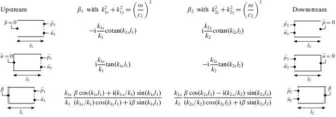
Table 4. Downstream admittance  $\unicode[STIX]{x1D6FD}_{2}=\bar{\unicode[STIX]{x1D70C}}_{2}c_{2}\tilde{u} _{2}/\tilde{p}_{2}$ seen by a flame sheet at $x=0$ for a chamber exhausting in a tube. Here, $c_{3}=c_{2}=c$, $k_{2}=k_{3}=k$. Helmholtz mode wavenumber: $k_{H}^{2}=S_{3}/(V_{2}l_{3})$.


