


1. Introduction
Liquid atomisation refers to the process where a bulk volume of liquid disintegrates into fragments featuring various sizes and shapes (Guildenbecher, López-Rivera & Sojka Reference Guildenbecher, López-Rivera and Sojka2009; Pairetti et al. Reference Pairetti, Popinet, Damián, Nigro and Zaleski2018). The fragments generated are described as sprays, which are involved in many natural and industrial processes, including ocean–atmosphere interactions (Veron Reference Veron2015; Erinin et al. Reference Erinin, Wang, Liu, Towle, Liu and Duncan2019), precipitation and rain-drop dynamics (Villermaux & Bossa Reference Villermaux and Bossa2009; Jalaal & Mehravaran Reference Jalaal and Mehravaran2012; Veron Reference Veron2015), combustion of liquid propellant in aerospace applications (Young Reference Young1995), pharmaceutical spray generation (Mehta et al. Reference Mehta, Haj-Ahmad, Rasekh, Arshad, Smith, van der Merwe, Li, Chang and Ahmad2017) and pathogen transmission (Bourouiba Reference Bourouiba2021; Kant et al. Reference Kant, Pairetti, Saade, Popinet, Zaleski and Lohse2022), etc. More specifically, it has recently been found that the atomisation of small-scale sea surface perturbations dominates ocean spume generation under extreme wind conditions, producing large droplets with typical sizes of  $10^2 \sim 10^3 \ \mathrm {\mu } {\rm m}$ (Troitskaya et al. Reference Troitskaya, Kandaurov, Ermakova, Kozlov, Sergeev and Zilitinkevich2017, Reference Troitskaya, Kandaurov, Ermakova, Kozlov, Sergeev and Zilitinkevich2018). In this size range the currently available sea-spray generation functions (SSGFs), crucial for calculations of air–sea momentum and heat exchange in Earth-system modelling, show a large range of scatter (Veron Reference Veron2015). However, since the physics governing the fragmentation of bag films have not yet been firmly established, their influences on SSGFs have been difficult to quantify. Improving this understanding is the primary motivation of the present work.
Two stages of liquid atomisation have been identified within literature, namely the primary and secondary atomisation. Sheets, ligaments and droplets are stripped from a bulk fluid during primary atomisation, which further decompose until stabilising capillary effects take over during secondary atomisation (Pairetti et al. Reference Pairetti, Popinet, Damián, Nigro and Zaleski2018). Secondary atomisation is typically modelled by the droplet aerobreakup problem characterised by the interaction between an initially spherical droplet with density  $\rho _l$, viscosity $\mu _l$ and diameter $d_0$, and an ambient gas flow with density $\rho _a$, viscosity $\mu _a$ and uniform velocity $U_0$ (Guildenbecher et al. Reference Guildenbecher, López-Rivera and Sojka2009). Based on these physical properties, together with surface tension $\sigma$ at the liquid–gas interface, four non-dimensional controlling parameters have been proposed using Buckingham's Pi theorem (see e.g. table 1 in Jalaal & Mehravaran Reference Jalaal and Mehravaran2014)
 \begin{equation} We \equiv \frac{\rho_a U_0^2 d_0}{\sigma}, \quad Oh \equiv \frac{\mu_l}{\sqrt{\rho_l d_0 \sigma}}, \quad \rho^* \equiv \frac{\rho_l}{\rho_a}, \quad \mu^* \equiv \frac{\mu_l}{\mu_a}. \end{equation}
Among these,  $We$ and $Oh$ are respectively the Weber and Ohnesorge number quantifying the ratio of inertial to capillary and viscous to capillary forces, and $\rho ^*$ and $\mu ^*$ are respectively the density and viscosity ratios of the liquid and gas phases.
Within the literature, various droplet aerobreakup regimes have been observed where the droplet shows different deformation patterns, and the transition thresholds between these regimes have traditionally been delineated using  $We$ and $Oh$ (Yang et al. Reference Yang, Jia, Che, Sun and Wang2017; Zotova et al. Reference Zotova, Troitskaya, Sergeev and Kandaurov2019; Marcotte & Zaleski Reference Marcotte and Zaleski2019), although some recent works have shown that the density ratio $\rho ^*$ may also play an important role (Yang et al. Reference Yang, Jia, Sun and Wang2016; Jain et al. Reference Jain, Tyagi, Prakash, Ravikrishna and Tomar2019; Marcotte & Zaleski Reference Marcotte and Zaleski2019). The value of $Oh$ has been reported to influence the transition thresholds only when exceeding a critical value of 0.1 (Hsiang & Faeth Reference Hsiang and Faeth1995); and as $We$ increases, the breakup becomes more violent and vibrational, bag, multi-mode (bag-stamen), sheet-thinning and catastrophic breakup regimes are observed in succession (Jalaal & Mehravaran Reference Jalaal and Mehravaran2014; Kékesi, Amberg & Wittberg Reference Kékesi, Amberg and Wittberg2014). Alternatively, based on the governing hydrodynamic instability involved in the process, the four breakup regimes mentioned above can be re-grouped into two major categories: Rayleigh–Taylor piercing and shear-induced entrainment (SIE) (Theofanous Reference Theofanous2011). However, despite the extensive amount of related work, the underlying physics governing the transient drop deformation in each regime are still largely unclear. Furthermore, the empirical transition criteria proposed so far are often contradictory (Theofanous Reference Theofanous2011; Yang et al. Reference Yang, Jia, Che, Sun and Wang2017), with the notable exception of a consensus that the critical Weber number beyond which bag breakup initiates is ${We}_c = 11 \pm 2$ when $Oh < 0.1$ (Guildenbecher et al. Reference Guildenbecher, López-Rivera and Sojka2009; Yang et al. Reference Yang, Jia, Che, Sun and Wang2017).
In the bag breakup regime, the initially spherical droplet first flattens and forms a disc, whose centre is then blown downstream and inflates into a hollow bag attached to a toroidal rim. The time it takes for the drop to reach breakup  $\Delta t_d$ typically falls within the range of $\tau \leqslant \Delta t_d \leqslant 2\tau$, where $\tau \equiv \sqrt {\rho _l / \rho _a} d_0 / U_0$ is the characteristic deformation time proposed by Nicholls & Ranger (Reference Nicholls and Ranger1969). The swollen bag first ruptures near its centre, triggering expansion of holes on the surface of the bag and eventually bursting into a large number of fragments, which is then followed by the breakup of the remnant toroidal rim into smaller numbers of fragments (Chou & Faeth Reference Chou and Faeth1998; Guildenbecher et al. Reference Guildenbecher, López-Rivera and Sojka2009; Opfer et al. Reference Opfer, Roisman, Venzmer, Klostermann and Tropea2014). Droplet bag breakup and its associated fragment size and velocity distribution functions are of specific interest as they bear a strong resemblance to the previously mentioned bag-mediated fragmentation of small-scale sea surface perturbations under extreme wind conditions (Troitskaya et al. Reference Troitskaya, Kandaurov, Ermakova, Kozlov, Sergeev and Zilitinkevich2017, Reference Troitskaya, Kandaurov, Ermakova, Kozlov, Sergeev and Zilitinkevich2018).
Droplet aerobreakup involves a complex interplay of aerodynamic, capillary and viscous effects that is still poorly understood (Jain et al. Reference Jain, Prakash, Tomar and Ravikrishna2015). The prevalent theoretical understanding is that hydrodynamic instabilities, particularly Kelvin–Helmholtz (KH) and Rayleigh–Taylor (RT) instability, play an important role in the aerobreakup process (Guildenbecher et al. Reference Guildenbecher, López-Rivera and Sojka2009; Theofanous Reference Theofanous2011; Theofanous et al. Reference Theofanous, Mitkin, Ng, Chang, Deng and Sushchikh2012; Jackiw & Ashgriz Reference Jackiw and Ashgriz2021). The KH instability occurs at the interface between two different streams of fluid with different velocities and densities (Kundu, Cohen & Dowling Reference Kundu, Cohen and Dowling2012). In the context of large- $We$ droplet aerobreakup, it governs the SIE breakup category (Theofanous Reference Theofanous2011), and is typically found near the drop periphery where the relative velocity between the liquid and gas phases is the largest (Gorokhovski & Herrmann Reference Gorokhovski and Herrmann2008; Jalaal & Mehravaran Reference Jalaal and Mehravaran2014). However, due to strong capillary effects, KH instability is unable to influence droplet deformation in the bag breakup regime (Theofanous et al. Reference Theofanous, Mitkin, Ng, Chang, Deng and Sushchikh2012; Jalaal & Mehravaran Reference Jalaal and Mehravaran2014). The RT instability occurs when a corrugated interface separating fluids with different densities undergoes constant acceleration (Zhou et al. Reference Zhou, Williams, Ramaprabhu, Groom, Thornber, Hillier, Mostert, Rollin, Balachandar and Powell2021), and is hypothesised to cause interfacial perturbation growth on the windward surface of the droplet. The wavenumber of such perturbations determines whether the droplet undergoes oscillatory deformation, bag breakup or multi-mode breakup (Yang et al. Reference Yang, Jia, Che, Sun and Wang2017). However, instability theories have difficulty in accounting for the viscous effects (Jalaal & Mehravaran Reference Jalaal and Mehravaran2014), flow dynamics prior to drop flattening and finite thickness and peripheral boundary of the flattened disc (Jackiw & Ashgriz Reference Jackiw and Ashgriz2021). Alternatively, some works highlight the influence of the internal flow within the droplets on the deformation process (Guildenbecher et al. Reference Guildenbecher, López-Rivera and Sojka2009; Villermaux & Bossa Reference Villermaux and Bossa2009; Jackiw & Ashgriz Reference Jackiw and Ashgriz2021; Obenauf & Sojka Reference Obenauf and Sojka2021; Ling & Mahmood Reference Ling and Mahmood2023). The internal flow model compensates for the drawback of the RT instability model in predicting early-time drop deformation; however, this approach is somewhat simplified and cannot account for the complex interaction between wake vortices and drop surface (Marcotte & Zaleski Reference Marcotte and Zaleski2019). The late-time breakup behaviour, on the other hand, is delineated into a bag film rupturing event, and the fragmentation of the remnant rim at a later time. The bag film rupture occurs more rapidly and produces much smaller fragments compared with the remnant rim breakup, and is thus more difficult to capture (Guildenbecher et al. Reference Guildenbecher, López-Rivera and Sojka2009). It has only recently been clarified experimentally (Jackiw & Ashgriz Reference Jackiw and Ashgriz2022) that the major pathways leading to bag fragmentation are the destabilisation and collision of hole rims as they recede over the curved bag and experience centripetal acceleration, which is also observed in the numerical simulations of Ling & Mahmood (Reference Ling and Mahmood2023), where they investigated in detail the morphological changes of the droplet in the moderate $We$ regime, and benchmarked them against existing theoretical and experimental results, based on which they improved the internal flow model of Jackiw & Ashgriz (Reference Jackiw and Ashgriz2021) for prediction of drop deformation. Nevertheless, ensemble-averaged size and velocity statistics of aerobreakup fragments are still scarce (Zhao et al. Reference Zhao, Liu, Xu and Li2011) and, given the large span in time and length scales, the understanding of what types of physical mechanisms are involved in the bag film breakup process and how each of them contributes to the statistics of fragments and dictates their subsequent behaviour remains unsatisfactory. Furthermore, the effects of the $Oh$ value on the bag breakup phenomena still remain largely unexplored (Jackiw & Ashgriz Reference Jackiw and Ashgriz2022).
The earliest research on droplet aerobreakup is mostly experimental, where the droplet breakup behaviour is recorded and analysed using shadowgraphs, high-speed cameras and particle image velocimetry (Hsiang & Faeth Reference Hsiang and Faeth1992; Guildenbecher et al. Reference Guildenbecher, López-Rivera and Sojka2009; Jalaal & Mehravaran Reference Jalaal and Mehravaran2012; Radhakrishna et al. Reference Radhakrishna, Shang, Yao, Chen and Sojka2021). Thanks to the recent development of computational power, numerical studies have provided a way to investigate atomisation phenomena and gain insight into fundamental mechanisms that are otherwise difficult to achieve experimentally (Gorokhovski & Herrmann Reference Gorokhovski and Herrmann2008; Ling, Zaleski & Scardovelli Reference Ling, Zaleski and Scardovelli2015). However, serious challenges are also present for computational studies on droplet aerobreakup, including reaching numerical convergence at large density ratio  $\rho ^*$ (Marcotte & Zaleski Reference Marcotte and Zaleski2019; Zotova et al. Reference Zotova, Troitskaya, Sergeev and Kandaurov2019) and the high computational cost of fully resolving small-scale fragmentation processes in two-phase turbulence simulations at high $We$ values (Gorokhovski & Herrmann Reference Gorokhovski and Herrmann2008; Jalaal & Mehravaran Reference Jalaal and Mehravaran2014; Shinjo Reference Shinjo2018), where the smallest droplet size may be much less than the Kolmogorov scale (Shinjo Reference Shinjo2018). There is also potential need of ensemble averaging when fragments produced from an individual realisation are not sufficient for obtaining statistically meaningful results (Mostert, Popinet & Deike Reference Mostert, Popinet and Deike2022). In particular, as the Navier–Stokes equations do not describe the physical mechanisms that control topological changes at phase boundaries, thin films are subject to uncontrolled numerical perforation when their thickness approaches the minimum grid size (Chirco et al. Reference Chirco, Maarek, Popinet and Zaleski2022). As a result, the fragment statistics are dependent on grid sizes (Jackiw & Ashgriz Reference Jackiw and Ashgriz2022), and numerical convergence with respect to bag fragment statistics has not previously been obtained to our knowledge. It is therefore of paramount importance to improve the grid resolution level and make the onset of breakup independent of the grid size, even though the exact physical mechanism initiating the breakup events remains elusive (Kant et al. Reference Kant, Pairetti, Saade, Popinet, Zaleski and Lohse2022). A few attempts have been made to improve the numerical resolution of fragmentation or coalescence phenomena. Among these, Coyajee & Boersma (Reference Coyajee and Boersma2009) first proposed a modified volume-of-fluid (VOF) scheme that utilises multiple marker functions for different fluid interfaces to minimise spurious coalescence on coarse meshes. Afterwards, Zhang, Chen & Ni (Reference Zhang, Chen and Ni2019) built a topology-based numerical scheme which automatically refines grid cells containing the liquid film bordered by two adjacent bubble interfaces. Finally, Chirco et al. (Reference Chirco, Maarek, Popinet and Zaleski2022) developed an algorithm that randomly perforates thin films once their thickness reduces to a prescribed critical value independent of the grid size. This algorithm is controllable via a set of tuning parameters and has been shown to improve grid convergence behaviour for various two-phase problems including droplet aerobreakup.
We present results of novel multiphase direct numerical simulation of droplet bag breakup using both axisymmetric and fully three-dimensional configurations. We conduct axisymmetric simulations to study pre-breakup deformation dynamics, and three-dimensional studies coupled with the manifold death (MD) algorithm of Chirco et al. (Reference Chirco, Maarek, Popinet and Zaleski2022) to shed light on the breakup dynamics of bag films and acquire statistics of bag film fragments for further analysis of their behaviour, while leaving the validation of the MD algorithm with appropriately tuned parameters for the aerobreakup problem to future work.
Our study is structured as follows. We present in § 2.1 the configuration of our problem and the parameter space we explore, and then introduce the numerical method in § 2.2. We analyse the axisymmetric simulation results in § 3 and compare them with previous theoretical predictions, focusing on the early-time deformation period where Jackiw & Ashgriz (Reference Jackiw and Ashgriz2021) predicted a constant spanwise growth rate (§3.1), and the film-thinning period immediately before bag breakup where an exponential decay model of film thickness is available (Villermaux & Bossa Reference Villermaux and Bossa2009) (§ 3.2). We then investigate the breakup of the bag film based on the three-dimensional simulation results, where we first show grid convergence of fragment statistics using the MD algorithm (Chirco et al. Reference Chirco, Maarek, Popinet and Zaleski2022) (§4.1). We then analyse the size and velocity distributions, and provide an overview of the breakup mechanisms leading to bag disintegration in § 4.2. Afterwards, we track and reconstruct the evolution of individual fragments, and study the dependence of their ejection velocity, lifetime and oscillation patterns in § 4.3. Finally, we investigate the influence of  $Oh$ values on the breakup of bag films (§ 4.4). We provide a summary for the numerical convergence of bag fragment statistics in § 5, and conclude the study in § 6 with some remarks on future work.
2. Formulation and methodology
2.1. Problem description
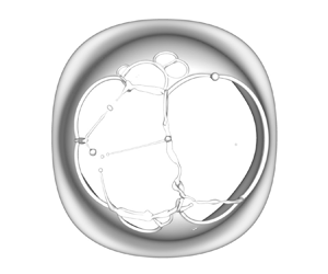
The flow configurations for axisymmetric and three-dimensional simulations are shown in figures 1(a) and 1(b), respectively. For both axisymmetric and three-dimensional simulations, a stationary liquid droplet with diameter  $d_0$, density $\rho _l$ and viscosity $\mu _l$ is placed close to the left boundary, surrounded by an initially quiescent gas phase with density $\rho _a$ and viscosity $\mu _a$. The domain width $D$ is set as $10d_0$ and $15d_0$ for axisymmetric and three-dimensional simulations, respectively, so as to eliminate the influence of finite domain size on the aerobreakup process. A zero-gradient velocity boundary condition is applied at the right boundary and a uniform incoming velocity $U_0$ is imposed on the left boundary, while no-penetration conditions are applied at the other domain boundaries. This velocity initialisation results in an impulsive acceleration of the droplet at the first time step, and induces a flow field satisfying both the incompressible constraint and the conservation of linear momentum (Jalaal & Mehravaran Reference Jalaal and Mehravaran2014; Marcotte & Zaleski Reference Marcotte and Zaleski2019).

Figure 1. Sketches showing the initial configurations of axisymmetric (a) and three-dimensional (b) droplet aerobreakup simulations. The axis of symmetry is located at the bottom in (a).
As discussed in § 1, the problem is defined by four non-dimensional parameters, namely the Weber number  $We$, the Ohnesorge number $Oh$, the density ratio $\rho ^*$ and the viscosity ratio $\mu ^*$. Since we are interested in air–water systems, $\rho ^*$ and $\mu ^*$ are set as 830 and 55, respectively, following the earlier work of Pairetti et al. (Reference Pairetti, Popinet, Damián, Nigro and Zaleski2018). We vary $We$ between 12 and 25 in our axisymmetric simulations, while in our current three-dimensional (3-D) simulations we fix it at 15. In the meantime, $Oh$ is varied between $10^{-4}$ and $0.075$, which allows for a comprehensive investigation of viscous effects on bag breakup.
2.2. Numerical method
We use the open-source Basilisk numerical library (Popinet Reference Popinet2019) to solve the Navier–Stokes equations for two-phase incompressible, immiscible and isothermal flows, which are written in the following variable-density form:
 \begin{gather} \boldsymbol{\nabla}\boldsymbol{\cdot} \boldsymbol{u} =0, \end{gather}
 \begin{gather}\rho \left( \frac{\partial \boldsymbol{u}}{\partial t} + \boldsymbol{u} \boldsymbol{\cdot}\boldsymbol{\nabla} \boldsymbol{u} \right) ={-}\boldsymbol{\nabla} p + \boldsymbol{\nabla}\boldsymbol{\cdot}\left[ \mu (\boldsymbol{\nabla} \boldsymbol{u} + \boldsymbol{\nabla} \boldsymbol{u}^T) \right] + \sigma \kappa \delta_s \boldsymbol{n}. \end{gather}
Equations (2.1) and (2.2) are respectively the continuity and momentum equation, where  $p$ is the fluid pressure. Surface-tension effects are incorporated in the volumetric form $\sigma \kappa \delta _s \boldsymbol {n}$ within (2.2), where $\sigma$ is the surface-tension coefficient, and $\kappa$ and $\boldsymbol {n}$ are respectively the local curvature and normal vector on the interface. The Dirac delta $\delta _s$ is non-zero only on the interface, indicating the local concentration of surface-tension effects (Popinet Reference Popinet2009, Reference Popinet2018).
The geometric VOF method is applied in Basilisk to reconstruct the interface and minimise the parasitic currents induced by surface tension (Popinet Reference Popinet2018), which solves the following advective equation:
 \begin{equation} \frac{\partial f}{\partial t} + \boldsymbol{u} \boldsymbol{\cdot}\boldsymbol{\nabla} f=0, \end{equation}
where  $f$ is the VOF function that distinguishes the liquid and gaseous phases, taking the value of 1 and 0 in the former and latter respectively. For modelling of surface-tension effects, $\delta _s \boldsymbol {n}$ in (2.2) is approximated as the gradient of the VOF function $\boldsymbol {\nabla } f$ using an adaptation of Brackbill's method (Brackbill, Kothe & Zemach Reference Brackbill, Kothe and Zemach1992; Popinet Reference Popinet2009), and the curvature $\kappa$ is calculated by taking the finite-difference discretisation of the derivatives of interface height functions (Popinet Reference Popinet2009). The quad/octree-based adaptive mesh refinement (AMR) scheme based on the estimation of local discretisation errors of the VOF function gradient $\boldsymbol {\nabla } f$ and flow velocity $\boldsymbol {u}$ is adopted so as to reduce the computational cost at high resolution levels $L$, which is defined using the minimum grid size
 \begin{equation} \varDelta = \frac{D}{2^L}. \end{equation}
As  $\varDelta$ is the smallest length scale at which necks of thinning filaments can be represented, $L$ sets the length scale at which liquid filament breakup occurs.
In the bag breakup regime, the onset of fragmentation is preceded by the inflation of bag structure whose thickness reduces considerably over time. While the mechanism responsible for the puncture of the bag film has been extensively discussed (Lhuissier & Villermaux Reference Lhuissier and Villermaux2012; Chirco et al. Reference Chirco, Maarek, Popinet and Zaleski2022; Kant et al. Reference Kant, Pairetti, Saade, Popinet, Zaleski and Lohse2022), in VOF simulations this is initiated when the local thickness of the bag decreases to the finest grid size (Ling et al. Reference Ling, Fuster, Zaleski and Tryggvason2017), causing the initiation time of breakup and the size of the finest fragments to be grid dependent. To circumvent this unphysical and numerically uncontrolled phenomenon, we adopt the MD algorithm recently developed by Chirco et al. (Reference Chirco, Maarek, Popinet and Zaleski2022), which artificially perforates thin films once their thickness decreases to a prescribed critical value independent of the grid size. This enables grid convergence to be reached in the fragment size distributions and related quantities (Chirco et al. Reference Chirco, Maarek, Popinet and Zaleski2022). This is realised in the Basilisk framework by first computing quadratic moments of the VOF colour function  $f$ on grid cells with a given signature level $L_{sig} \leqslant L$, which defines the critical thickness $h_c \equiv 3D/2^{L_{sig}}$, the smallest length scale at which liquid films can be presented as below it they will be artificially perforated by the MD algorithm. The signs of the computed quadratic moments indicate the local shape of the interface. If a film with thickness not larger than $h_c$ is detected, the algorithm randomly creates cubic cavities on the ligament by directly setting the value of $f$ to that of the other phase with a probability $p_{perf}$. While the total fluid mass is changed when holes are created on thin films, the MD algorithm is able to minimise this side effect by creating cavities with minimum sizes that allow for Taylor–Culick expansion, and limiting the maximum number of holes perforated at every iteration. Further discussion, and details of the parameters used for the MD algorithm in our study are supplied in § 4.1.
Before the formation of thin bag films and their subsequent breakup, the smallest length scale in the aerobreakup problem is the thickness of the viscous air boundary layer  $\delta$ around the droplet, through which momentum diffuses from the surrounding airflow into the droplet and drives its deformation. Batchelor's estimation with the defining length scale of the droplet $d_0$ yields $\delta \sim d_0 / \sqrt {Re}$, where $Re \equiv \rho _a U_0 d_0/\mu _a$ is the free-stream Reynolds number. For a typical droplet in the bag breakup regime, characterised by Weber and Ohnesorge numbers $We = 15$, $Oh = 10^{-3}$, this corresponds to $\delta \sim 1.2 \times 10^{-2} d_0$. The recommended criteria of $\delta /\varDelta \geqslant 2$ (Mostert & Deike Reference Mostert and Deike2020) then requires that the grid resolution level satisfies $L \geqslant 12$ for simulations with domain size $D = 15 d_0$. The highest grid resolution level we set in our present simulations is $L = 14$, at which the droplet contour in our axisymmetric simulations has reached grid independence. The numerical convergence of fragment statistics will be discussed in detail in § 4.1.
Finally, the droplet diameter  $d_0$, incoming flow velocity $U_0$, dynamic flow pressure $p_0 \equiv \rho _l U_0^2$ and the characteristic deformation time $\tau$ introduced in § 1 provide the natural reference scales for the length, mass and time quantities that appear in (2.1) and (2.2), and will be used to non-dimensionalise the numerical results in the remainder of this study unless otherwise specified.
3. Pre-breakup deformation dynamics
Before the onset of bag breakup, the shape of the deforming droplet remains largely axisymmetric, although the wake region may have become fully turbulent and three-dimensional. Many previous numerical aerobreakup studies therefore conducted axisymmetric simulations for a parametric study (Yang et al. Reference Yang, Jia, Che, Sun and Wang2017; Jain et al. Reference Jain, Tyagi, Prakash, Ravikrishna and Tomar2019; Marcotte & Zaleski Reference Marcotte and Zaleski2019). In this section, we present our axisymmetric results to provide an overview of the pre-breakup deformation characteristics of the droplet, while also verifying our simulation results by comparing with available analytic models and experimental results.
3.1. Early-time deformation
We first discuss the initiation period of aerobreakup, defined by Jackiw & Ashgriz (Reference Jackiw and Ashgriz2021) as  $0 \leqslant t \leqslant T_i$, where $T_i$ is the time when the droplet reaches its minimal streamwise thickness. To provide an overview of the early-time droplet deformation process characterised by spanwise flattening, we first present in figure 2 the droplet contours extracted from our axisymmetric simulations at various instants within $0 \leqslant t/\tau \leqslant 0.8$ for two different Ohnesorge numbers $Oh$ of $10^{-3}$ and $10^{-2}$, while the same Weber number $We = 15$ is set for both cases. The radial profile is shown with $y=0$ as the axis of symmetry. It is found that during the early deformation stage, the windward surface of the droplet continues moving downstream and pushing liquid to the drop periphery, leading to the gradual spanwise flattening of the droplet. In the meantime, a dimple develops on the windward surface that moves downwards and eventually evolves into a crater on the axis of symmetry for $Oh = 10^{-3}$, as shown in figure 2(a). The leeward side of the droplet remains relatively stationary after an initial movement to the left. In contrast, figure 2(b) shows that the increase of $Oh$ to $10^{-2}$ postpones the dimple formation on the windward surface significantly, which only begins to appear at $t/\tau = 0.8$. Previous works have attributed the spanwise flattening of the drop to the aerodynamic pressure difference between the frontal stagnation point and the equatorial periphery (Jackiw & Ashgriz Reference Jackiw and Ashgriz2021), which drives the internal flow within the droplet against the restoring effects of surface tension (Marcotte & Zaleski Reference Marcotte and Zaleski2019). The airflow quickly separates from the leeward surface, creating a re-circulation region with low pressure which induces little movement at the leeward interface (Jain et al. Reference Jain, Prakash, Tomar and Ravikrishna2015). Formation of similar dimple structures on the windward surface can also be observed in figure 1 of Marcotte & Zaleski (Reference Marcotte and Zaleski2019) within the Weber number range of $11.3 \leqslant We \leqslant 24$ corresponding to bag and bag-stamen breakup.

Figure 2. Early-time development of droplet contours for axisymmetric simulations with Ohnesorge number  $Oh = 10^{-3}$ (a) and $10^{-2}$ (b), while the Weber number $We=15$. The axis of symmetry is at $y=0$.
We briefly examine whether the dimple is a result of RT instability developing on the windward surface due to wind acceleration. Li, Zhang & Kang (Reference Li, Zhang and Kang2019) predicted a critical instantaneous Bond number  $Bo_c \equiv \rho _l \alpha d_0^2/4\sigma = 11.2$, beyond which the windward surface is destabilised. Here, $\alpha$ is the instantaneous acceleration of the liquid droplet. For a droplet with $We = 15$, $Oh = 10^{-3}$, our results show $Bo = 0.57$ at $t/\tau = 0.4$ when the dimple is first observed in figure 2(a), much smaller than the threshold value of 11.2 predicted by Li et al. (Reference Li, Zhang and Kang2019). Taking into account that the liquid is being primarily pushed from the frontal stagnation point to the windward side of the periphery around the time of dimple formation ( $t/\tau \sim 0.4$ in figure 2a), together with the $We$ range where it is observed in Marcotte & Zaleski (Reference Marcotte and Zaleski2019), it is more likely that the dimple formation is caused by the capillary pinching effects against fluid influx, and should therefore be viewed as a precursor of later rim formation.
For validation of our numerical results, we present in figure 3 the evolution of the maximum spanwise radius of the drop  $R_m$ and the streamwise length of the bag $L_{bag}$ measured from our axisymmetric and 3-D numerical simulations at $We = 15$, $Oh = 2.5 \times 10^{-3}$, and compare them with the available experimental results of Jackiw & Ashgriz (Reference Jackiw and Ashgriz2021) and Flock et al. (Reference Flock, Guildenbecher, Chen, Sojka and Bauer2012). It can first be seen that the axisymmetric and 3-D numerical results agree excellently until $t \approx 1.5\tau$, when the axisymmetric simulation shows a smaller bag length in figure 3(b). This late-time deviation most likely arises from the lack of 3-D flow instability development in axisymmetric simulations (Marcotte & Zaleski Reference Marcotte and Zaleski2019), which may break the symmetry of the bag and limits its streamwise growth. Both our axisymmetric and 3-D simulation results agree well with the experimental data of Jackiw & Ashgriz (Reference Jackiw and Ashgriz2021) up to $t/\tau = 1$, after which the experimental results show faster growth in both $R_m$ and $L_{bag}$. This may be due to the sensitivity of the flattened drop to difference in the ambient flow conditions, as in our numerical simulations the air-phase flow remains laminar, whereas the experimental configuration of Flock et al. (Reference Flock, Guildenbecher, Chen, Sojka and Bauer2012) and Jackiw & Ashgriz (Reference Jackiw and Ashgriz2021) in fact produces air-phase turbulence, which has been shown by Zhao et al. (Reference Zhao, Nguyen, Duke, Edgington-Mitchell, Soria, Liu and Honnery2019) to be capable of increasing the height and width of bags at late time (see e.g. their figure 6). More specifically, Jackiw & Ashgriz (Reference Jackiw and Ashgriz2021) used a 5 gauge air needle (whose diameter $D_n$ is only 2.48 times of the droplet diameter $d_0$) to generate air jets with centreline Reynolds number $Re_a$ of $5.2 \times 10^3 \sim 2.5 \times 10^4$, apart from needles for suspending the drop within such air jets. In the case of Flock et al. (Reference Flock, Guildenbecher, Chen, Sojka and Bauer2012), air jets are produced through a nozzle with diameter $D_n \approx 11d_0$, but the airflow is also turbulent with $Re_a = 1.8 \times 10^4$. The results of Jackiw & Ashgriz (Reference Jackiw and Ashgriz2022) are obtained from single experimental runs without being ensemble averaged, which may lead to larger variations in their results, as also noted in the comparison of numerical results by Ling & Mahmood (Reference Ling and Mahmood2023). Additionally, note that in figure 3(a), the experimental results of Jackiw & Ashgriz (Reference Jackiw and Ashgriz2021) and Flock et al. (Reference Flock, Guildenbecher, Chen, Sojka and Bauer2012) show some mutual disagreement in the spanwise radius values within the range of $t/\tau \leqslant 1.5$.

Figure 3. Comparison of our axisymmetric and 3-D simulation results for the evolution of bag length (a) and width (b) at  $We = 15$, $Oh = 2.5 \times 10^{-3}$ with the experimental data of Jackiw & Ashgriz (Reference Jackiw and Ashgriz2021) and Flock et al. (Reference Flock, Guildenbecher, Chen, Sojka and Bauer2012). The breakup lengths and widths for various $Oh$ values are included as scattered points, and the balance time $T_{bal} = 0.125\tau$ proposed by Jackiw & Ashgriz (Reference Jackiw and Ashgriz2021) is also plotted for reference.
The bag lengths and widths recorded at various  $Oh$ values at the point of breakup are also included as scattered points in figure 3, which we will return to in § 4.4. It can be seen that our bags approach breakup within the time range of $1.74 \leqslant t/\tau \leqslant 1.91$, earlier than the experimental results of Jackiw & Ashgriz (Reference Jackiw and Ashgriz2021) ( $t = 2.2\tau$ for $We = 15.3$). On the other hand, Flock et al. (Reference Flock, Guildenbecher, Chen, Sojka and Bauer2012) did not report the exact time at which bag breakup is initiated. This earlier breakup time is associated with the limit of grid resolution, and hence $L_{sig}$ on the critical thickness at which the bag film is perforated by the MD algorithm, as at $L_{sig} = 13$, the critical thickness is $3D/2^{L_{sig}} = 5.5 \times 10^{-3} d_0$, which is a few times larger than the experimental value of $h/d_0 = 1.2 \times 10^{-3}$ as found by Jackiw & Ashgriz (Reference Jackiw and Ashgriz2022), and $5 \times 10^{-5} \leqslant h/d_0 \leqslant 5 \times 10^{-4}$ by Opfer et al. (Reference Opfer, Roisman, Venzmer, Klostermann and Tropea2014). This is a limitation present in all numerical simulations of droplet aerobreakup, as is also noted in the recent work of Ling & Mahmood (Reference Ling and Mahmood2023).
Furthermore, Jackiw & Ashgriz (Reference Jackiw and Ashgriz2021) found experimentally that there exists an early period featuring constant growth rate of the maximum spanwise radius of the droplet  $R_m$, and proposed the following model for its prediction
 \begin{equation} \dot{R} = \frac{d_0 T_{bal}}{8 \tau^2} \left( a^2 - \frac{128}{We} \right), \end{equation}
where  $a$ is the axial stretching rate near the frontal stagnation point and approximated as $a \simeq 6$; $\tau$ is the characteristic deformation time introduced in § 1; and $T_{bal}$ is the time when a constant streamwise deformation rate is reached, taken as $0.125 \tau$ according to the experimental results (Jackiw & Ashgriz Reference Jackiw and Ashgriz2021). We note that this model is derived assuming ellipsoidal or cylindrical droplet shape and a balance between aerodynamic and capillary forces during deformation, which leads to a purely radial internal velocity profile that cancels out the viscous effects.
We now investigate (3.1) using our axisymmetric numerical results. Figures 4(a) and 4(b) show respectively the influence of  $We$ and $Oh$ on the measured instantaneous spanwise growth rate $\tilde {\dot {R}}$, where the tilde indicates normalisation by the theoretical value (3.1). We also include the growth rate evolution obtained by numerically differentiating the experimental data presented in figure 28 of Jackiw & Ashgriz (Reference Jackiw and Ashgriz2021) for comparison. For the small $Oh$ value of $10^{-3}$, figure 4(a) indicates that the spanwise growth rate $\tilde {\dot {R}}$ reaches a plateau with relatively small variations around $t = 0.3 \tau$, where the prediction of (3.1) matches qualitatively with the measured $\tilde {\dot {R}}$ values. We note that while Jackiw & Ashgriz (Reference Jackiw and Ashgriz2021) set $T_{bal} = 0.125\tau$ as an a posteriori estimation based on the evolution of $R_m$ rather than $\tilde {\dot {R}}_m$ when analysing their figure 17(b), our results agree well with the spanwise growth rate computed from their experimental data up to $t = 0.74\tau$, with their data also reaching a plateau around $t = 0.3 \tau$. The growth rate of Jackiw & Ashgriz (Reference Jackiw and Ashgriz2021) becomes much larger than ours for $t > 0.74\tau$, corresponding to the larger $R_m$ values observed in figure 3(a), which is possibly a result of air-phase turbulence as previously discussed. For cases at $Oh = 10^{-3}$, this period of constant $\tilde {\dot {R}}$ ends around $t = 0.55 \tau$, after which $\tilde {\dot {R}}$ reaches a peak around $t = 0.6\tau$ and then decreases, indicating a deviation from model (3.1) absent in the analyses of Jackiw & Ashgriz (Reference Jackiw and Ashgriz2021). On the other hand, figure 4(b) suggests that as $Oh$ increases beyond $2.5 \times 10^{-3}$, the late-time peaking of $\tilde {\dot {R}}$ gradually attenuates, while the match with (3.1) is improved and maintained for longer periods of time, which is particularly interesting as (3.1) is derived based on inviscid flow assumptions and cannot account for viscous influences. Note that Jackiw & Ashgriz (Reference Jackiw and Ashgriz2021) tested droplets for which $Oh = 2.7 \times 10^{-3}$; our numerical results are therefore consistent with their experiment.

Figure 4. Measured droplet spanwise growth rate compared with the experimental data of Jackiw & Ashgriz (Reference Jackiw and Ashgriz2021). Evolution of instantaneous spanwise growth rate  $\tilde {\dot {R}}$ at various $We$ and $Oh = 10^{-3}$ (a) and various $Oh$ with $We = 15$ (b) are plotted; and the results are normalised using (3.1).
Returning to figure 2(a) suggests that, during the period  $0.3\tau \leqslant t \leqslant 0.55\tau$ when the constant growth rate $\tilde {\dot {R}}$ is observed, the liquid is being pushed from the frontal surface to the windward side of the periphery, where the maximum spanwise radius is reached. However, at $t = 0.6\tau$, when the peaking behaviour is observed, a bulge appears downstream and causes a location shift where the maximum spanwise radius $R$ is reached. This bulging behaviour is also present in the growth rate evolution computed from the experimental data of Jackiw & Ashgriz (Reference Jackiw and Ashgriz2021) at $Oh = 2.7 \times 10^{-3}$, but virtually absent when $Oh = 10^{-2}$ in our numerical simulations, as shown in figure 2(b), where the periphery of the droplet contour only flattens over time.
To provide insights into physical mechanisms governing the peak in the spanwise growth rate observed for low  $Oh$ values in figure 4, we plot in figure 5 the pressure distribution and streamlines near the drop periphery, when the peaks in the spanwise growth rate $\tilde {\dot {R}}$ are reached in figure 4(b) for $We = 20$, $Oh = 10^{-3}$ and $We = 15$, $Oh = 10^{-2}$. It can be seen that the surrounding gas flow separates from the droplet surface at the windward side of the periphery, creating attached recirculating vortices in its wake with low pressure and slow fluid motion (Jain et al. Reference Jain, Tyagi, Prakash, Ravikrishna and Tomar2019; Marcotte & Zaleski Reference Marcotte and Zaleski2019), where the bulges are located. The pressure difference in the surrounding flow between the frontal stagnation point and the recirculating region drives the internal flow within the droplet from the windward surface to the periphery. Furthermore, the peaks in $\tilde {\dot {R}}$ observed when $Oh \leqslant 0.005$ are associated with the formation of a high-pressure region at the bulge on the droplet periphery, as can be seen in figure 5(a), which is caused by surface tension and decelerates the flow into the bulge. Further development of the bulge leads to an increase in the local capillary pressure, which causes the decrease in $\tilde {\dot {R}}$ after the peak. Notably, the droplet contour in figure 5(b) at $Oh = 10^{-2}$ lacks craters at the axis of symmetry and bulges at the periphery, and therefore more closely resembles the cylindrical shape of the deforming drop assumed in the derivations of (Jackiw & Ashgriz Reference Jackiw and Ashgriz2021), which may explain why the match with the inviscid model (3.1) is improved as $Oh$ is increased.

Figure 5. Flow fields near the tip of a droplet with  $We = 20$, $Oh = 10^{-3}$ (a) and $We = 15$, $Oh = 10^{-2}$ (b) when the peaks in $\dot {R}$ are reached. The non-dimensional times at which (a,b) are taken are respectively $t/\tau = 0.62$ and 0.66.
We further investigate the distribution patterns of flow pressure and velocity in the vicinity of the droplet, and their association with prediction (3.1) of Jackiw & Ashgriz (Reference Jackiw and Ashgriz2021). Figure 6(a) shows the air- and liquid-phase pressure on either side of the drop surface as functions of the arclength  $l$ traversing along the axisymmetric droplet contour in the clockwise direction. It can be seen that at very early time $(t/\tau = 5 \times 10^{-2})$, the air-phase pressure profile closely follows the sinusoidal potential-flow solution for $l/d_0 \leqslant 0.6$, which corresponds to the windward face of the drop; whereas the profile at $l/d_0 > 0.6$ deviates from the potential-flow solution due to flow separation, characterised by a second minimum around $l/d_0 = 1.2$. We also note that at $t/\tau = 5 \times 10^{-2}$ the shape of the liquid-phase pressure profile bears strong resemblance to its air-phase counterpart, with a nearly uniform upshift due to the constant capillary pressure difference $4\sigma /d_0$. As the droplet flattens over time, the air-phase pressure profile on the windward surface increases and the first minimum moves upstream, deviating from the potential-flow solution. In the meantime, the change in liquid-phase pressure for $l/d_0 \leqslant 0.37$ is relatively small, and the air- and liquid-phase pressure profiles cross over each other at $l/d_0 = 0.37$ and $t/\tau = 0.4$, signalling the dimple formation on the windward surface as the local radius of curvature reaches infinity. It is also noted that the minimum of the liquid-phase pressure profile around $l/d_0 = 0.85$ observed at $t/\tau = 0.4$ becomes a maximum at $t/\tau = 0.6$, which corresponds to the bulge formation observed in figure 5(a) that leads to the deviation from (3.1) (Jackiw & Ashgriz Reference Jackiw and Ashgriz2021).

Figure 6. (a) Evolution of air ( $p_a$, solid lines) and liquid pressures ( $p_w$, dotted lines) on either side of the droplet interface as functions of the interfacial arc length $l$; (b) axial airflow velocity $u_z$ on the axis of symmetry as a function of the distance to the windward stagnation point of the droplet $z$. The values of $We$ and $Oh$ are respectively 15 and $10^{-3}$.
Figure 6(b) shows the air-phase axial velocity  $u_x$ measured on the axis of symmetry as a function of the distance to the windward stagnation point of the drop $z/d_0$, where the slope of the curves corresponds to the axial stretching rate $a$ used in model (3.1). It is first observed that the axial velocity value at $z/d_0 = 0$ increases gradually over time, which is because the measuring point is located in the air-phase boundary layer attached to the accelerating droplet. The axial stretching rate $a$ is found to gradually decrease from 6 and approach $4/{\rm \pi}$, the extreme values corresponding to spherical and pancake drop shapes as noted in Jackiw & Ashgriz (Reference Jackiw and Ashgriz2021); crossing over the intermediate value of $2\sqrt {2}$ proposed by Kulkarni & Sojka (Reference Kulkarni and Sojka2014). The decrease of $a$ corresponds to the air-phase pressure increase on the windward surface as observed in figure 6(a) via the following equation:
 \begin{equation} p_g(r) - p_g(0) ={-}\rho_g \frac{a^2U_0^2}{8d_0^2}r^2. \end{equation}
 Consequently, we conclude that our numerical results reproduce the prediction (3.1) of Jackiw & Ashgriz (Reference Jackiw and Ashgriz2021) that there exists a period characterised by a constant spanwise radius growth rate  $\tilde {\dot {R}}$. Furthermore, we find that the later deviation from (3.1) is characterised by a peak in $\tilde {\dot {R}}$, which is caused by the capillary deceleration of liquid influx into the drop periphery that causes bulge formation at low $Oh$ values. The increase in $Oh$ eliminates the bulge and the frontal crater on the droplet surface, and the droplet acquires a nearly cylindrical shape which is one of the underlying assumptions by Jackiw & Ashgriz (Reference Jackiw and Ashgriz2021) when deriving (3.1), hence the better match with their model.
3.2. Film drainage and onset of bag breakup
When the droplet deforms into a disc at the end of the early-time deformation period, corrugations develop on their frontal surfaces which have generally been considered as RT perturbation waves (Yang et al. Reference Yang, Jia, Che, Sun and Wang2017). This appears in figure 7(a) at  $t/\tau =0.95$, $We=15$, in the form of waves on the windward surface of the droplet. Later on, thick rims are observed to form at the drop periphery due to capillary pinching effects, which extract liquid from the drop centre and contribute to the formation of bag films near the axis of symmetry. Subject to the aerodynamic pressure difference between their frontal and leeward surfaces, these films further bulge out from the rim (Jackiw & Ashgriz Reference Jackiw and Ashgriz2021) and cause exponential growth of streamwise bag length before breakup.

Figure 7. (a) Evolution of axisymmetric droplet contours with  $We = 15$ and $Oh=10^{-3}$, where the axis of symmetry is at $y=0$. (b) Droplet contours at $t/\tau = 1.73$ with various $Oh$ values and $We = 15$.
Figure 7(a) shows non-uniform profiles of the bag thickness  $h$, featuring a neck where a local minimum in $h$ is reached and the film breakup eventually occurs. The neck moves outwards radially at $We = 15$, leaving a thickening remnant stamen structure developing at the axis of symmetry (Marcotte & Zaleski Reference Marcotte and Zaleski2019). Figure 7(b), on the other hand, shows the deformed drop contours at $t/\tau = 1.73$ for various $Oh$ values; and it can be seen that as $Oh$ increases, the neck becomes less obvious as the distribution of bag film thickness becomes more uniform.
It has been argued that the breakup of bag films is due to an RT instability peculiar to thin films rather than a finite-time singularity of the Navier–Stokes equations (Villermaux & Bossa Reference Villermaux and Bossa2009). Assuming inviscid flow and uniform bag thickness, Villermaux & Bossa (Reference Villermaux and Bossa2009) derived the following exponential decay model for the film thickness  $h$:
$h$:
 \begin{equation} h(t) \sim d_0 {\rm e}^{-\lambda t}, \end{equation}
where the exponential decay rate  $\lambda$ is given as $4/\tau$. We compare our numerical results with the predictions of model (3.3) in figure 8. The film thickness $h$ is calculated by measuring the minimum distance between the windward and leeward surfaces of the deformed drop contour over a time period of $t_b - 0.87\tau \leqslant t \leqslant t_b$, where $t_b$ is the time when film breakup is detected. Logarithmic scale is used for the $y$ axis to facilitate comparison of the decay rate $\lambda$.

Figure 8. The evolution of film thickness  $h$ for $t_b - 0.87\tau \leqslant t \leqslant t_b$, measured from simulations with various $We$ with $Oh = 10^{-3}$ (a) and various $Oh$ with $We = 15$ (b). For a droplet with $We = 15$, $Oh = 0.001$, the breakup time is $t_b/\tau = 1.84$, and $t_b - 0.87\tau = 0.97\tau$. As figure 7(a) shows, over this period a bag is blown out from the centre of the flattened disc. Villermaux and Bossa's prediction (3.3) is also plotted for comparison.
It can be seen that, for the  $We$ and $Oh$ range presented in figure 8, the exponential decay rate $\lambda$ is initially close to the prediction of (3.3). This phase, which features a constant thickness decay rate, roughly corresponds to the period of rim development prior to the ‘bulging’ of bag films, which is shown in figure 7. However, the decay rate increases as the film continues thinning and approaches breakup, similar to the result of Kant et al. (Reference Kant, Pairetti, Saade, Popinet, Zaleski and Lohse2022), which becomes more significant as $We$ and $Oh$ decrease. Most notably, at $We = 12$ the thinning rate continuously increases close to the onset of breakup, which suggests that an exponential decay law in the form of (3.3) does not fully capture the underlying physics for film drainage with strong surface tension.
Developing new theoretical models in place of (3.3) whose predictions match better with the late-time neck drainage behaviour observed within the  $We$ and $Oh$ range of interest is out of the scope of the current work. We note briefly that the drainage behaviour of bag films under the influence of aerodynamic pressure difference observed here bears resemblance to the drainage of liquid films between a free air–water surface and a buoyancy-driven air bubble (Pigeonneau & Sellier Reference Pigeonneau and Sellier2011; Kočárková, Rouyer & Pigeonneau Reference Kočárková, Rouyer and Pigeonneau2013; Guémas, Sellier & Pigeonneau Reference Guémas, Sellier and Pigeonneau2015), where film drainage models are developed based on lubrication assumptions (see § 4.2 of Magnaudet & Mercier (Reference Magnaudet and Mercier2020) and references therein for more detailed discussions). More specifically, Pigeonneau & Sellier (Reference Pigeonneau and Sellier2011) also showed a deviation from exponential decay of bubble film thickness under asymptotically large surface tension, which is ascribed to a finite-time singularity and contrasts with the thin-film RT instability mechanism proposed by Villermaux & Bossa (Reference Villermaux and Bossa2009). However, the major difference between the bag and the bubble film drainage problem lies in the location of the neck. For the drainage of bag films, the neck can be formed some distance away from the axis of symmetry due to a competition of inertia between the outer rim and the inner stamen (Marcotte & Zaleski Reference Marcotte and Zaleski2019), which complicates theoretical modelling due to additional difficulties in predicting time-varying neck locations. In contrast, bubble film drainage always occurs on the axis of symmetry, as the thin bubble film is connected to an infinitely large and quiescent liquid domain.
4. Breakup of bag films
In this section, we analyse our 3-D simulation results during the period when the bag film undergoes disintegration to form small fragments, and the axisymmetric flow assumption completely breaks down. It is noted that the late stage of aerobreakup is not covered when the receding remnant bag collides with the surrounding main rim and triggers the fragmentation of the latter (Jackiw & Ashgriz Reference Jackiw and Ashgriz2022), which will be reserved for future work.
4.1. Grid convergence for fragment statistics
While the physical mechanisms responsible for the onset of liquid film breakup in general remain an active research topic, with various candidates proposed including chemical or thermal inhomogeneities (Kant et al. Reference Kant, Pairetti, Saade, Popinet, Zaleski and Lohse2022), Marangoni effects (Lhuissier & Villermaux Reference Lhuissier and Villermaux2012) or presence of surface contamination (Néel & Villermaux Reference Néel and Villermaux2018), it has been argued that for bag films under normal acceleration, thickness modulations arise across the film due to the RT instability, resulting in perforation when the perturbation amplitude becomes comparable to the film thickness  $h$ (Villermaux & Bossa Reference Villermaux and Bossa2009; Jackiw & Ashgriz Reference Jackiw and Ashgriz2021).
Numerically, the perforation and subsequent fragmentation of thin films in droplet breakup problems has historically been challenging to represent in a physically consistent manner. Given that perforation involves a topological change in the air–water interface, numerical studies have usually employed interface-capturing techniques such as the geometric VOF approach employed here (Jain et al. Reference Jain, Prakash, Tomar and Ravikrishna2015, Reference Jain, Tyagi, Prakash, Ravikrishna and Tomar2019; Tang et al. Reference Tang, Mostert, Fuster and Deike2021); such methods can represent interfacial topological change without a need for extensive special treatment. However, such techniques also tend to suffer from an unphysical and numerically uncontrolled perforation and fragmentation mode in thin films, which moreover compromises numerical convergence of the statistics of the resulting fragment populations (Chirco et al. Reference Chirco, Maarek, Popinet and Zaleski2022). In this phenomenon, when the film thickness approaches the local mesh size, it begins to destabilise, generating a large number of small fragments without a well-defined fragmentation mechanism; figure 9(a) shows a qualitative illustration of this phenomenon in our own simulations. This phenomenon also appears in images of droplet breakup in Jain et al. (Reference Jain, Prakash, Tomar and Ravikrishna2015); unfortunately, information on numerical convergence of fragment statistics is not supplied in that study.

Figure 9. Effect of the MD algorithm on the bag breakup behaviour at grid level  $L=12$ and 13 for $We = 15$, $Oh = 10^{-3}$. (a–c) Simulation snapshots showing fragmenting bag films at $t/\tau = 1.909$ without (a) and with artificial perforation (b,c). The grid resolution level is $L=12$ for (a,b) and 13 for (c), while the MD signature level for (b,c) is $L_{sig} = 12$.
The MD algorithm constructed and implemented by Chirco et al. (Reference Chirco, Maarek, Popinet and Zaleski2022) into Basilisk aims to bypass this spurious mode of fragmentation. This algorithm detects and artificially perforates thin films periodically by removing liquid mass once their thickness decreases to a prescribed critical value. The key point is that VOF breakup is circumvented because the film is perforated at a thickness greater than what is required for VOF breakup to occur. A limitation of the MD method is that it removes mass from the droplet in order to generate the hole, which disturbs the momentum and mass conservation properties of the VOF scheme as implemented in Basilisk. We find in practice that the parameters of the MD algorithm can be adjusted so that sufficiently few holes are formed in these simulations and this mass loss becomes insignificant (see below).
The holes created by the MD perforation mechanism resemble those appearing in experiments (such as Lhuissier & Villermaux Reference Lhuissier and Villermaux2013; Jackiw & Ashgriz Reference Jackiw and Ashgriz2022; Kant et al. Reference Kant, Pairetti, Saade, Popinet, Zaleski and Lohse2022) – see figure 9(b). The algorithm also affords considerable user control over the frequency and location, for example, of the perforations. In the present study, we control perforation frequency using a probabilistic approach which is scaled to be independent of parallelisation, resolution and the calling interval of the algorithm, in order to minimise the number of free parameters governing the perforation problem. The appropriate choice of probability to match the efficiency of hole generation in experimental studies, such as those seen in Lhuissier & Villermaux (Reference Lhuissier and Villermaux2012) and Vledouts et al. (Reference Vledouts, Quinard, Vandenberghe and Villermaux2016), is a complicated problem which is left for future work. Our aim in this study is instead to establish numerical convergence and verify various aspects of the resulting fragmentation process with experiment and theory, which in our knowledge has not been established in previous numerical studies.
All grid convergence test cases we conduct in this section are reloaded from a single 3-D simulation snapshot with an intact bag at  $We = 15$, $Oh = 10^{-3}$ and the perforation probability and calling interval for the MD algorithm are set as $p_{perf} = 5.7 \times 10^{-5}$ and $\Delta t_c = 0.5d_0/U_0$, with grid level $L = 12$, 13, 14 and signature level $L_{sig} = 11$, 12, 13 (see § 2 for their definition). The fragment statistics are collected and output at fixed time intervals until the bags have fully disintegrated, and then post-processed to obtain time- and/or ensemble-averaged data. It is noted that as the test cases run without using the MD algorithm are deterministic in the sense that VOF breakup appears repeatably in the same locations of the thin film, while producing a large number of very small fragments, only one realisation is completed at each $L$ value; whereas the MD algorithm introduces randomness in the perforation location and subsequent fragment formation, while also reducing the number of fragments, and therefore multiple realisations are completed for a given set of $L$ and $L_{sig}$ to generate sufficient total number of fragments for ensemble averaging. A full list for the configurations of the 3-D numerical simulations is available in table 1.
Table 1. List of ensemble realisations for 3-D numerical simulations carried out in this work, where the drop Weber and Ohnesorge numbers  $We$ and $Oh$, the grid and signature levels $L$ and $L_{sig}$, the number of individual realisations and the purpose for using the ensemble data (the grid convergence study for §§ 4.1 and 4.2, or the $Oh$ effect study in § 4.4) are indicated.

We first demonstrate the effects of the MD algorithm on the breakup behaviour of the bag film in figure 9. The film rupture behaviour is qualitatively different with and without application of the MD algorithm. Figure 9(a) is a snapshot for a simulation case run without using the MD algorithm, featuring numerous small-scale irregular corrugations and ligament breaking on the bag, which reflect the uncontrolled nature of VOF breakup. Figures 9(b) and 9(c) show that the MD algorithm is able to create holes on the bag film in a controlled manner, and reduce the influence of VOF breakup on the bag dynamics. These holes created by the MD algorithm feature well-defined bordering rims that recede over the bag and create surface capillary waves ahead of them, and these may collide with one another and form a few long stretching liquid bridges (Agbaglah Reference Agbaglah2021), which are distinct from the numerous short and irregular bridges observed with VOF breakup. Note that figure 9(b) still shows some VOF breakup behaviour which is absent in figure 9(c). This reflects the fact that, even though the film is perforated when the film thickness reaches the order of  $3\varDelta _{sig}$, the perforation probability and the rate of hole expansion are sufficiently low such that there are regions of the film that continue to thin down to the order of $\varDelta$, where VOF breakup begins. In figure 9(b), $\varDelta = \varDelta _{sig}$, so that VOF-induced fragmentation still appears, but this can be further minimised by choosing $L > L_{sig}$, such as in figure 9(c).
Figure 10 further compares the grid convergence behaviour for the size and velocity distribution of bag fragments without and with the MD algorithm applied. The fragment data are sampled at different times throughout the bag film breakup period, and then collected and binned based on the equivalent fragment diameter  $d$ to produce the size and velocity distribution functions. While the distribution functions presented in figures 10(a)–10(d) are for single realisations, those in figures 10(e)–10(f) are ensemble averaged for each bin over different realisations; and we have verified that the total number of bins does not significantly influence the shape of size and velocity distributions. Figure 10(a) shows the fragment size distribution functions obtained from individual simulations without application of the MD algorithm. It can be seen that, while the distributions have similar shapes at various grid levels $L$, i.e. featuring large number densities of small fragments near the minimum grid size, followed by a fall off at large fragment sizes, there is no clear indication of the distribution functions reaching grid convergence. In particular, it is observed that, as $L$ increases, the entire size distribution shifts to smaller sizes. In contrast, figure 10(c) presents the fragment size distribution functions obtained from individual realisations within the range of $13 \leqslant L \leqslant 14$ and $11 \leqslant L_{sig} \leqslant 13$ when the MD algorithm is used. While more scatters in the size distribution functions are seen when compared with figure 10(a) due to smaller amounts of fragments produced, we no longer observe the shift to small fragment sizes for the distribution tail with $d \geqslant 8\varDelta _{sig}$, which is the range for well-resolved fragments as observed by Chirco et al. (Reference Chirco, Maarek, Popinet and Zaleski2022); and size distributions at different grid and signature levels appear to overlap for $d \geqslant 8\varDelta _{sig}$ despite these scatters. Figure 10(e) further presents the ensemble-averaged size distribution functions obtained with the MD algorithm applied, which features much smaller range of scatter, as indicated by the confidence bounds represented by the grey shade at $L=14$, $L_{sig} = 13$, showing clearly that the distributions of fragment statistics overlap for $d \geqslant 8\varDelta _{sig}$ at different values of $L$ and $L_{sig}$. From this we conclude that the ensemble-averaged data are grid converged for $d \geqslant 8\varDelta _{sig}$ and $13 \leqslant L \leqslant 14, L > L_{sig}$. Moreover, together figures 10(a), 10(c) and 10(e) establish that the lack of grid convergence in the no-MD case (figure 10a) is attributable not to the scatter of individual realisations, but specifically to numerically uncontrolled VOF breakup.

Figure 10. Time- and ensemble-averaged size (a,c,e) and speed (b,d,f) probability distribution functions of aerobreakup fragments obtained from simulations without using the MD algorithm (a,b), from an individual realisation (c,d) and from ensemble-averaged data across various realisations with the MD algorithm applied (e,f) at various grid resolution and signature levels. Confidence bounds for each bin are computed across different ensemble realisations at  $L=14$, $L_{sig} = 13$ using the bootstrapping method, and plotted in (e,f) using shaded area. For all test cases, $We = 15$ and $Oh = 10^{-3}$.
We also include the experimental data of Guildenbecher et al. (Reference Guildenbecher, Gao, Chen and Sojka2017) obtained with  $We = 13.8$ and $Oh = 5.43\times 10^{-3}$ in figure 11, together with exponential and log-normal models fitted to their data. Guildenbecher et al. (Reference Guildenbecher, Gao, Chen and Sojka2017) noted the difference between the size distributions obtained using two experimental techniques with different resolution levels, and expressed most confidence in the upper tail of the distributions satisfying $d \geqslant 0.01 d_0$. Within this size range, the tails of our size distribution and those of Guildenbecher et al. (Reference Guildenbecher, Gao, Chen and Sojka2017) show excellent agreement, which further validates our numerical results within the size range of $d \geqslant 8\varDelta _{sig}$. While we leave for future work the detailed investigation of possible differences in fragmentation mechanisms between our present results and the experiments of Guildenbecher et al. (Reference Guildenbecher, Gao, Chen and Sojka2017) and Jackiw & Ashgriz (Reference Jackiw and Ashgriz2021, Reference Jackiw and Ashgriz2022), the present remarkable agreement with experimental data at larger fragment sizes suggests that the upper tails of the size distribution do not depend on whatever these differences may be. Both the exponential and the log-normal model are found to match well with the current size distribution functions for $d \geqslant 8\varDelta$, while both differ from the current results within the range of $d < 8\varDelta$, which may suggest that no single function can represent the complete spectrum of the current size distribution of bag fragments.

Figure 11. Fragment size distribution function measured from our  $L = 14$, $L_{sig} = 13$ simulations, compared with the experimental data of Guildenbecher et al. (Reference Guildenbecher, Gao, Chen and Sojka2017) measured at two different apparatus resolutions. A zoom-in view is provided as an inset to facilitate comparison of different size distribution functions within the size range of $0.01 \leqslant d/d_0 \leqslant 0.1$. Exponential and log-normal functions fitted to the experimental size distribution function are also included.
It is noted that, in figure 10(e), the fragment statistics are not fully converged for  $d \leqslant 8\varDelta _{sig}$, where compared with its counterparts at $L=13$, the size distribution at $L=14$ shows more fragments satisfying $\varDelta \leqslant d \leqslant \varDelta _{sig}$, and fewer fragments with $\varDelta _{sig} \leqslant d \leqslant 8\varDelta _{sig}$. This is probably because the fragments within this range are primarily formed due to the breakup of liquid ligaments, especially the smallest fragments near the grid size, which are most likely the satellite drops produced from the capillary breakup of corrugated slender ligaments (Pal et al. Reference Pal, Crialesi-Esposito, Fuster and Zaleski2021). These are controlled by the grid level $L$ rather than the signature level $L_{sig}$, as the geometry-specific MD algorithm only targets thin liquid films in 3-D simulations and does not act in the stretch-induced breakup of liquid ligaments. Our numerical results for $d \leqslant 8\varDelta _{sig}$ also deviate from the log-normal function fit of Guildenbecher et al. (Reference Guildenbecher, Gao, Chen and Sojka2017), which may be due to multiple factors including the difference in $We$, the presence of additional flow perturbations in experiments, and possibly resolution limits in experimental equipment, as exemplified by a comparison performed in figure 9 of Guildenbecher et al. (Reference Guildenbecher, Gao, Chen and Sojka2017). On the other hand, the size distribution function of very large fragments satisfying $d \geqslant 0.1 d_0$ show relatively larger range of scatter compared with their smaller counterparts around $8\varDelta _{sig}$, which likely arises from the smaller number of these fragments produced in each ensemble realisation and can be further reduced by increasing the ensemble size. Finally, we remark that the influence of MD on mass conservation is minimal as the loss of liquid mass incurred by the MD algorithm does not exceed 0.023 % for $t/\tau \leqslant 2.18$ at $L=13$ and 14.
Figures 10(b), 10(d) and 10(f) show the average speed  $\bar {v}$ of fragments as functions of the fragment diameter $d$ obtained from simulations without and with the MD algorithm applied. Similar to the size distribution functions, the shapes of the distribution of $\bar {v}$ clearly indicate grid convergence for the tail constituted by the well-resolved fragments with $d \geqslant 8\varDelta _{sig}$ in figure 10(f), which is not observed in figure 10(b) where large scatters across various grid levels are present. Interestingly, in figure 10(f), fragments with diameter $d \geqslant 8\varDelta _{sig}$ show little variation in the average speed, which appears to be a constant independent of the values of $L$ and $L_{sig}$; whereas a peak can be observed within the range of $\varDelta _{sig} \leqslant d \leqslant 8\varDelta _{sig}$ which is grid dependent, along with the large increase of the speed of tiny fragments close to $\varDelta _{sig}$ which approaches the free-stream velocity $U_0$. While it is clear therefore that the production mechanisms of droplets satisfying $d \leqslant 8\varDelta _{sig}$ may not be grid converged, the resulting dynamics of these small droplets turns out to be well resolved; more detailed analysis establishing this will follow in § 4.2.
In summary, our results in this section demonstrate that the application of the MD algorithm helps to establish grid convergence of fragment size and speed statistics for well-resolved fragments with diameter  $d \geqslant 8\varDelta _{sig}$, which is not achieved when VOF breakup is dominant. Based on these results, all following 3-D studies of bag film breakup are conducted at $L = 14$ and $L_{sig} = 13$.
4.2. Mechanisms leading to bag fragmentation
In this section, we further analyse the fragment statistics obtained from our grid convergence tests run at  $L = 14$ and $L_{sig} = 13$, to provide insight into the shapes of the size and distribution functions observed in § 4.1, and the physical mechanisms governing the formation of fragments and their subsequent evolution patterns. These choices of $L$ and $L_{sig}$, together with the MD parameters specified in § 4.1, allow the creation of only a few holes on the bag film, which is not only enough to avoid the onset of VOF breakup, but also preserves abundant film breakup phenomena including rim recession, collision and destabilisation behaviour that would otherwise be hard to recover with more holes created, where rim collision would dominate (Vledouts et al. Reference Vledouts, Quinard, Vandenberghe and Villermaux2016). As is noted in § 3.1, our film is thicker and breaks up earlier compared with experimental results due to the limit of grid resolution. This leads to smaller Taylor–Culick velocity values, which reduces the probability of destabilisation of receding liquid rims (Jackiw & Ashgriz Reference Jackiw and Ashgriz2022) and production of fine drops (Néel & Villermaux Reference Néel and Villermaux2018); but our results show that many interesting breakup mechanisms can already be captured with this choice of $L_{sig}$, which we will present further below.
We first show in figure 12 the time evolution of the instantaneous distributions of the size, axial and radial speed distributions of the fragments produced from bag breakup. Figure 12(a) indicates that, immediately after the onset of bag breakup ( $t/\tau = 1.96$), only small fragments close to the minimum grid size are produced, and well-resolved larger fragments satisfying $d \geqslant 8\varDelta _{sig}$ only come into existence as time elapses, and are always fewer compared with small fragments near the grid size. The shape of the size distribution function gradually stabilises, and reaches a steady state by $t/\tau = 2.11$ that is very close to the ensemble- and time-averaged size distribution function. These findings suggest that the smaller and larger fragments are produced through different physical mechanisms that arise at different stages of bag breakup, and eventually these fragmentation mechanisms die out as the bag approaches full disintegration and the fragment size distribution is well represented by time-averaged results. The remaining rim will then disintegrate at still later times, whose investigation we leave for future work.

Figure 12. Ensemble-averaged instantaneous size distribution functions (a), and probability distribution functions of axial (b) and radial (c) speed of aerobreakup fragments calculated at  $L = 14$ and $L_{sig} = 13$. Ensemble- and time-averaged fragment size distribution function is also plotted in (a) for reference.
Figures 12(b) and 12(c) show the instantaneous distribution of fragment axial and radial speeds  $u_x$ and $u_r \equiv \sqrt {u_y^2 + u_z^2}$ as functions of their sizes, with the ensemble-wide variations of velocity components in each averaging bin shown in error bars. It can be seen that the speed of well-resolved fragments satisfying $d \geqslant 8\varDelta _{sig}$ remains close to a constant value without significant variations. While the statistics of smaller fragments with $d \leqslant 8\varDelta _{sig}$ are not fully numerically converged, they do show considerably larger variation around the binned average value in qualitative agreement with the experimental results of Guildenbecher et al. (Reference Guildenbecher, Gao, Chen and Sojka2017). Interestingly, we observe peaks around $d/d_0 = 5 \times 10^{-3}$ in the distributions of both $u_x$ and $u_r$, whose location does not appear to vary with time. Moreover, despite the presence of velocity variations, figure 12(b) suggests that the average axial speed $u_x$ of smaller fragments with $d \leqslant 8\varDelta _{sig}$ increases over time, whereas the radial speed $u_r$ does not show similar increasing trend in figure 12(c). This is most likely because the smaller fragments are generated earlier and therefore are exposed to the airflow for much longer periods of time compared with larger fragments; together with their smaller mass, this means that they are much more easily accelerated by the axial velocity component of the airflow, hence the continuous increase in their $u_x$ values. On the other hand, $u_r$ does not increase significantly over time, likely because the airflow in the wake region does not have a large radial velocity component that can accelerate bag fragments as they migrate downstream.
We will hereafter discuss qualitatively several mechanisms through which the bag film undergoes fragmentation and form small droplets, which can be identified by inspecting typical simulation snapshots taken from our  $L = 14$, $L_{sig} = 13$ simulations. Firstly, figure 13 shows the breakup of a stretched long ligament neighbouring two enlarging holes into a series of small drops. As the ligament is itself connected to the main drop, there is a significant size difference between the parent and child drops produced from its breakup, which is an example of non-local breakup events (see (4.3) in § 4.3 for a definition of non-local breakup). It can be seen from figure 13(a) that significant cross-sectional diameter variations have developed on the ligament before the onset of its breakup, which can be viewed as the result of the nonlinear development of the RP instability (Pal et al. Reference Pal, Crialesi-Esposito, Fuster and Zaleski2021). Afterwards, the ligament shrinks to form sharp tips and then breaks up on multiple sites, as shown in figure 13(b), and forms a primary drop which continues to undergo periodic prolate–oblate shape oscillations resembling droplets produced by breaking Rayleigh jets (Hu et al. Reference Hu, She, Fang, Su and Fu2021), as highlighted in the red boxes in figures 13(b)–13(h). This is because the pinch-off of the stretching ligament induces an inner velocity field within the detaching droplet that drives it in the oblate direction (see e.g. figure 7(b) in Hu et al. Reference Hu, She, Fang, Su and Fu2021), matching the perturbation shape of the second Rayleigh mode, which then excites oscillation modulated by capillary effects. In the meantime, the other parts of the ligament do not pinch off to form a series of fragments at once, but first break up into several elongated debris, and then split into large primary and small satellite drops via the well-known end-pinching mechanism (Castrejón-Pita, Castrejón-Pita & Hutchings Reference Castrejón-Pita, Castrejón-Pita and Hutchings2012; Pal et al. Reference Pal, Crialesi-Esposito, Fuster and Zaleski2021), which is an example of local breakup events as the parent (the elongated debris) and child (satellite drops) do not differ significantly in their sizes. Under certain circumstances, the primary and satellite drops might coalesce and form a larger fragment as highlighted in the blue boxes, resembling the ‘immediate satellite merge’ mechanism discussed by Vassallo & Ashgriz (Reference Vassallo and Ashgriz1991).

Figure 13. Snapshots showing the non-local breakup of a long ligament into multiple fragments during bag film fragmentation with  $We = 15$ and $Oh = 10^{-3}$. The red boxes show formation of a single fragment through non-local end pinching and its subsequent oscillation, and the blue boxes show the formation of two fragments through a local breakup event and their subsequent coalescence.
Figure 14 first shows an example of short ligament breakup and its eventual contraction into a single droplet, as highlighted in the blue boxes. Compared with the breakup of long ligaments demonstrated in figure 13, this type of short ligament breakup bears stronger resemblance to the breakup phenomena of liquid bridges studied by Agbaglah (Reference Agbaglah2021), where fragments produced from the same liquid bridge do not feature significant size variations. This is most likely because the initial holes are placed very close to each other in Agbaglah (Reference Agbaglah2021), and the receding rim does not have enough time to grow in size and momentum before their impact.

Figure 14. Snapshots showing the detachment of a liquid node from ligament webs (highlighted in the red box) and the evolution of a short ligament into a single drop (highlighted in the blue box) during bag film fragmentation with  $We = 15$ and $Oh = 10^{-3}$.
Another type of fragmentation mechanism can also be identified in figure 14; as highlighted in the red boxes, three adjacent holes have merged with each other, and their three bordering rims converge on a common ‘node’ as they are stretched, which is also observed in the breakup of ligament webs formed on Savart sheets by Lhuissier & Villermaux (Reference Lhuissier and Villermaux2013). Compared with the ligament pinch-off mechanism discussed earlier, the surface evolution of this ‘node’ shows much more complicated corrugation patterns as the rims it was connected to are gradually detached, and therefore is not dominated by the second Rayleigh mode alone. The ‘node’ drop that eventually forms in this case also has a much larger size compared with its counterparts formed from ligament pinch-off events. However, different from an earlier study by Vledouts et al. (Reference Vledouts, Quinard, Vandenberghe and Villermaux2016), our choice of  $L = 14$ and $L_{sig} = 13$ does not produce holes on the bag film with as high a number density, and therefore we are not able to directly measure the wavelength of the RT instability responsible for the film fragmentation from the average distance between the centres of adjacent holes. The relatively smaller number density of holes formed also means that the larger ‘node’ drops formed due to the merging of three or more adjacent and similarly sized holes are relatively rare compared with generally smaller fragments formed from ligament breakup, which require the collision of only two adjacent liquid rims. Furthermore, no less than three holes should fully expand and arrive at the same region on the bag film where the node is located, and each of the connecting rims need to break off successively before the node can be treated as a separate fragment by the fragment counting algorithm. These factors help explain the tail of the size distribution function of aerobreakup fragments taking shape at much later time as we observed in figure 12(a); namely, that larger droplets are relatively few, and produced at generally later times during the fragmentation process.
We also note that, while we often observe the formation, oscillation and subsequent corrugation development of liquid ligaments after the impact of receding rims, as shown on the ligament to the left of the red box in figure 14, destabilisation of such structure due to the RT instability and its subsequent evolution into fully developed transverse ‘fingers’ and ‘fine drops’ are only occasionally observed in our current simulations. According to Néel, Lhuissier & Villermaux (Reference Néel, Lhuissier and Villermaux2020), these two regimes are separated by a critical local Weber number for rim collision  $We_c \equiv \rho _l (2v_{TC})^2 d_l / \sigma = 66$, where $d_l$ is the rim diameter. Neglecting the curved geometry of the bag film, liquid mass conservation further yields $We_c = 8 \sqrt {D_c/{\rm \pi} h}$, where $D_c$ and $h$ are respectively the distance between the centre of two neighbouring holes and the film thickness. Taking $h = 3D/2^{L_{sig}} = 3D/2^{13}$, we find that $We_c = 66$ corresponds to $D_c = 1.2 d_0$, which we expect might be reached for some pairs of sufficiently separated holes, as the bag diameter $d_f$ before the onset of fragmentation typically approaches $2d_0$, as shown in both our numerical results and the experimental data of Jackiw & Ashgriz (Reference Jackiw and Ashgriz2021) (see e.g. their figure 30). Figure 15 highlights two such examples in red boxes, where we observe the transverse growth of the lamella and the growth of finger-shaped corrugations on its edges; however, before the fingers fully develop and detach as ‘fine’ drops, holes are observed to form on the thinning lamella, which then expand and collide with the fingering lamella edges, turning them into isolated breaking ligaments. Similar phenomena of lamellae rupture and their edges forming corrugated ligaments can also be observed in figure 14 of Vledouts et al. (Reference Vledouts, Quinard, Vandenberghe and Villermaux2016), although in that case the lamellae appear to remain within the plane of the film surface, and do not experience transverse growth; and VOF breakup may play a role in the present examples. Nevertheless, the liquid ligaments found in the current simulations have already displayed a variety of well-documented physical phenomena that collectively contribute to the large span of fragment sizes found in our fragment distribution functions.

Figure 15. Snapshots showing the evolution of ‘fingering’ liquid lamellae during bag film fragmentation with  $We = 15$ and $Oh = 10^{-3}$.
Lastly, we observed a few examples showing the destabilisation of receding liquid rims, as demonstrated in figure 16. These destabilisation phenomena are absent in the recent work of Agbaglah (Reference Agbaglah2021) where holes expand over a flat liquid film, and are therefore most likely linked with the influence of centrifugal acceleration caused by the curved bag film (Lhuissier & Villermaux Reference Lhuissier and Villermaux2012; Jackiw & Ashgriz Reference Jackiw and Ashgriz2022). While we are not yet able to measure the wavelength or the linear growth rate of the instability, and therefore have not identified the type of hydrodynamic instability involved here; we observe in figure 16(d) regular-spaced holes highlighted in the red boxes forming at the foot of the rim bordering the hole on the left. These are not attributable to VOF breakup because they are not observed to appear elsewhere on the bag at the same time; while the rim bordering the larger hole on the right is seen to develop regular corrugation patterns, which might be an indication that the receding liquid rim is experiencing the RP instability. Any further development of the instability is interrupted by the eventual collision between adjacent rims (not shown in figure 16). The readers are referred to Jackiw & Ashgriz (Reference Jackiw and Ashgriz2022) for a more comprehensive discussion on rim destabilisation. There a few candidates are proposed, including the RT instability mechanism governing the ‘fingering’ behaviour on bursting surface bubbles (Lhuissier & Villermaux Reference Lhuissier and Villermaux2012); and it is concluded that the centrifugal acceleration does not govern the instability of the rim directly, but instead regulates the thickness of the rim via a local-Bond-number criterion (Wang et al. Reference Wang, Dandekar, Bustos, Poulain and Bourouiba2018), with the rim in turn susceptible to the RP instability. With the present methodology, these rim instabilities can be investigated in more detail with higher signature levels  $L_{sig}$, and concomitantly higher $L$. Given the large computational expense of such simulations, it is not feasible to include such an analysis in the present study.

Figure 16. Snapshots showing the receding liquid rim destabilisation during bag film fragmentation with  $We = 15$ and $Oh = 10^{-3}$. The sites where the rim is detached from its base is highlighted in red boxes.
4.3. Behaviour of bag fragments
In the following, we move away from considering the dynamics and numerical characteristics of the production mechanisms of fragments to examine instead those of the fragments themselves. To provide further insight into the evolution of individual fragments rather than their collective behaviour, we utilise the droplet tracking algorithm proposed by Chan et al. (Reference Chan, Dodd, Johnson and Moin2021a) in post-processing to reconstruct their breakup lineage. This toolbox assumes breakup and coalescing events to be binary (i.e. at most two parent droplets may collide and form one large child droplet, or two child droplets may be produced from the breakup of one parent droplet in a single breakup/coalescing event), and is capable of identifying all coalesce/breakup events and differentiate between the new drops produced from these events and those which do not undergo such changes. It requires only the instantaneous fragment size, location and velocity output from the simulation at given time intervals, instead of knowledge of the entire flow field at successive simulation time steps, and therefore incur only limited computational cost (Chan et al. Reference Chan, Dodd, Johnson and Moin2021a).
As the fragments produced from bag breakup are much smaller compared with the parent drop, and therefore have a much smaller Weber number, it is highly unlikely that they will undergo another bag breakup event. However, they may still experience secondary breakup to form smaller fragments as they evolve over time. It is therefore of interest to determine the lifetime of breaking parent fragments  $T_p$ using the toolbox of Chan et al. (Reference Chan, Dodd, Johnson and Moin2021a), defined as the interval between their birth and death in two successive breakup events (Rivière et al. Reference Rivière, Ruth, Mostert, Deike and Perrard2022). Figure 17(a) shows $T_p$ as a function of the diameter $d_p$ of parent fragments, with the bin-averaged values of $T_p$ shown in grey squares. The solid dots plotted in the background represent recorded individual breakup events, and are colour coded by the logarithm value of the minimum child/parent diameter ratio $d_c/d_p$, highlighting a broad distribution of parent fragment lifetime. For comparison, the characteristic capillary time of fragments $t_{cap}$ is also plotted in figure 17(a) as a function of $d_p$, which is defined as follows:
 \begin{equation} t_{cap}(d_p) = \sqrt{\frac{\rho_l d_p^3}{8\sigma}}. \end{equation}
It can first be seen from the scattered original data that most of the bag film fragments that undergo a secondary breakup fall within the range of  $d_p \geqslant 8\varDelta _{sig}$, which corresponds to the ‘well resolved’ fragments discussed in § 4.1. Furthermore, the lifetime of fragments $T_p$ satisfying $d_p \leqslant 0.05d_0$ shows a dependency on $r_p$ that roughly scales with the characteristic capillary time, but this trend breaks down for even larger fragments with $d_p \geqslant 0.05d_0$. It is noted that the capillary time defined in (4.1) is proportional to the oscillation period of droplet spherical harmonic modes (4.4). Therefore, the scaling of $T_p$ with $t_{cap}$ for $d_p \leqslant 0.05d_0$ may suggest that the fragmentation of these fragments is primarily due to large-amplitude nonlinear oscillations which can trigger a capillary breakup (Lalanne, Masbernat & Risso Reference Lalanne, Masbernat and Risso2019). This also explains the large scatters we observe in the lifetime of parent fragments within this size range, as when nonlinearity becomes dominant, the surface oscillations cannot be represented by a single mode, and different modes of perturbation with different oscillation periods might trigger breakup depending on specific fragments. As for even larger fragments with $d_p \geqslant 0.05d_0$, their lifetime $T_p$ appears to scatter around an average value of $10t_{cap}(h_c)$, where $t_{cap}(h_c)$ is the characteristic capillary time based on the critical film thickness $h_c = 3D/2^{L_{sig}}$. Here, $10t_{cap}(h_c)$ is an estimation of the inertial time scale leading to the capillary breakup of stretching liquid ligaments, which are formed due to hole collision (Agbaglah Reference Agbaglah2021). This suggests that this type of non-local breakup is only dependent on the topological evolution of the stretching liquid ligament, rather than that of the entire parent drop from which the child fragments are torn off; but this remains to be verified in future work.

Figure 17. (a) The lifetime of the parent fragments  $T_p$ as a function of their diameter $d_p$, where $We = 15$ and $Oh = 10^{-3}$. The bin-averaged results are shown in grey hollow squares, and the original data are shown as solid dots, whose colour represents the value of the child/parent diameter ratio. It is noted that this plot does not include the main drop as a parent which features $d_p/d_0 \approx 1$. (b) Velocity difference between parent and child fragments $\varDelta u$ as a function of the child/parent diameter ratio $d_c/d_p$ is shown in the main plot, whereas the inset plot shows $\Delta u$ as a function of the diameter of child fragments $d_c$.
We were also able to compute the magnitude of the velocity differences  $\Delta u$ between fragment parents and their children at two successive instants when the fragment statistics are collected, and plot them in figure 17(b) as a function of the ratio between the child and parent diameter $d_c/d_p$. It is found that, for breakup events where a small child/parent size ratio $(d_c/d_p \leqslant 0.22)$ are detected, the velocity difference $\varDelta u$ appears to show little dependence on $d_c/d_p$, despite significant scatter. Based on our findings in figure 17(a), these breakup events with $d_c/d_p \leqslant 0.22$ mostly feature small children with large parents. On the other hand, breakup events satisfying $d_c/d_p \geqslant 0.22$ are dominated by small parents and children, and their $\Delta u$ decreases with increasing values of $d_c/d_p$, roughly following a power-law scaling $\Delta u \propto (d_c/d_p)^{-1.2}$. We further note that the $\Delta u$ values of breakup events satisfying $d_c/d_p \leqslant 0.22$ roughly coincides with the inviscid Taylor–Culick velocity $v_{TC}$, with an estimation for the bag film thickness $h$ based on the signature level $L_{sig}$
 \begin{equation} v_{TC} \equiv \sqrt{\frac{2\sigma}{\rho_l h}} = \sqrt{\frac{2^{L_{sig}+1} \sigma}{3\rho_l D}} \approx 0.17U_0. \end{equation}
This agrees with the recent confirmation by Néel & Deike (Reference Néel and Deike2022) that the speed of film drops produced from bubble bursting can be estimated by  $v_{TC}$ to an order of magnitude. An explanation for this approximate agreement is as follows. Prior and up to collision between adjacent hole rims, each rim travels at the Taylor–Culick velocity. The colliding rims of these holes then form liquid ligaments, which exhibit an axial stretching rate comparable to the pre-collision rim speed (i.e. the Taylor–Culick velocity). This stretching rate in turn sets the relative speed of sufficiently small fragments ejected from the parent ligament. The parent ligaments may constitute part of the parent drop, or may themselves have separated from it. Therefore, for a given child droplet size produced by this mechanism, the ratio $d_c/d_p$ may see considerable variation. Consequently, we observe the large range of $d_c/d_p \leqslant 10^{-2}$ where the parent/child velocity difference remains close to $v_{TC}$. The inset of figure 17(b) further shows the velocity difference in breakup events as a function of the child diameter $d_c$ alone; and this time we find that it is the small fragments satisfying $d_c \leqslant 8 \varDelta _{sig}$ that appear to approach $v_{TC}$, agreeing with our analysis that it is the fragments produced from liquid ligament breakup that are represented within the range of $d_c/d_p \leqslant 0.22$. Note, however, that, in the inset of figure 17(b), $\varDelta u$ continues to increase beyond $v_{TC}$ with decreasing $d_c$, and does not scatter around $v_{TC}$ as in the main plot. This is most likely because the droplet tracking algorithm has a finite fragment detection frequency (Chan et al. Reference Chan, Dodd, Johnson and Moin2021a), and the smallest fragments may be generated and accelerated by the ambient airflow between two successive instants when this algorithm is called for their detection. The nominal velocity difference $\Delta u$ for the smallest fragments therefore includes contributions from both the initial ejection velocity (primarily in the radial direction) and the increment due to airflow acceleration (primarily in the axial direction), which causes $\Delta u$ to increase steadily beyond $u_{TC}$. As these smallest fragments are scattered in different averaging bins according to the child/parent diameter ratio of the breakup events, the contribution of airflow acceleration to $\Delta u$ becomes less obvious.
Based on our findings in figure 17(b), we introduce the following criteria for determining ‘non-local’ breakup and coalescing events, respectively:
 \begin{equation} \max \left( \frac{d_{c,i}}{d_p} \right) \leqslant 0.22, \quad \max \left( \frac{d_c}{d_{p,i}} \right) \leqslant 4.64, \quad i = 1,2. \end{equation}
Otherwise we term the breakup or coalescing events ‘local’. Here, the critical child/parent diameter ratio of 0.22 for fragment breakup (and analogously 4.64 for coalescence) separates the two breakup regimes found in figure 17(b), where the velocity difference  $\Delta u$ either scatters around $v_{TC}$ or scales with $d_c/d_p$. Note that the term ‘local’ here does not mean the parent and child fragments are close to each other in terms of their locations in the physical space, which all such events satisfy, but rather in the sense of the parent and its two children being close in their respective sizes (Chan, Johnson & Moin Reference Chan, Johnson and Moin2021b).
We further plot in figure 18 the ensemble-averaged number density of breakup and coalescing events detected during the bag fragmentation period. It is found that both breakup and coalescing events occur most frequently around  $t/\tau = 2.10$. This is most likely when the receding rims fully absorb the bag film and collide with each other, which then triggers a series of corrugated ligament breakup and fragment coalescing events. After this the breakup and coalescing behaviour become less frequent, as the corrugated ligaments gradually disintegrate without liquid mass input from the bag film. While there exist ‘multistep’ breakup events in our aerobreakup simulation outputs, our results in figure 18 suggest that the fragmentation process involved in the aerobreakup problem cannot be well described by a breakup cascade model (Garrett, Li & Farmer Reference Garrett, Li and Farmer2000; Chan et al. Reference Chan, Johnson and Moin2021b), as non-local breakup and coalescing events producing children with sizes drastically different from their parents are found to dominate this problem, which is different from the entrained air bubble breakup scenario in breaking wave studies (Garrett et al. Reference Garrett, Li and Farmer2000; Deane & Stokes Reference Deane and Stokes2002; Deike, Melville & Popinet Reference Deike, Melville and Popinet2016; Chan et al. Reference Chan, Johnson and Moin2021b; Mostert et al. Reference Mostert, Popinet and Deike2022) where the prevalence of local breakup events leads to a well-defined bubble-mass flux supporting breakup cascade models. It is also noted that breakup events occur much more frequently than coalescing events for bag films, which is expected as the latter requires two adjacent fragments to cross paths at the same time, which only happen for a small portion of neighbouring fragments with specific initial position and velocity configurations.

Figure 18. Ensemble-averaged evolution of number of breakup (a) and coalesce (b) events during the breakup of bag films produced from an initial droplet with  $We = 15$ and $Oh = 10^{-3}$. All ensemble realisations are run at $L = 14$, $L_{sig} = 13$.
Apart from identifying all breakup and coalescing events in the spray formed due to aerobreakup, the toolbox developed by Chan et al. (Reference Chan, Dodd, Johnson and Moin2021a) also enables us to track the evolution of properties of individual fragments during their lifetime. For example, figure 19(a) shows the evolution of surface energy  $E_s$ of individual small fragments recorded from simulations run at $L=14$ and $L_{sig} = 13$, with the records of only a few representative fragments highlighted for clarity. The steady-state values of surface energy is also computed based on the volume of corresponding fragments, and plotted in grey dashed lines for reference. It is seen that the oscillation frequency and amplitude vary for each fragment, but all of them clearly demonstrate decaying oscillation behaviour, with their oscillation frequency generally increasing with decreasing fragment radius $r$ (hence decreasing steady-state surface energy values). We further extract the frequency of the dominant oscillation mode of these small fragments at two different grid resolution configurations ( $L = 14$, $L_{sig} = 13$ and $L = 13$, $L_{sig} = 11$), and plot them against the fragment radius in figure 19(b), where an excellent agreement is found for small fragments within the diameter range of $0.01d_0 \leqslant d \leqslant 0.1d_0$ with the theoretical predictions of Prosperetti (Reference Prosperetti1980) for the second Rayleigh mode, which is given as follows for an inviscid droplet with density $\rho _l$ and radius $R^*$ at equilibrium:
 \begin{equation} \omega_{n,0} = \sqrt{(n-1)n(n+2) \frac{\sigma}{\rho_l R^*}}, \end{equation}
where  $n$ is the spherical harmonic mode number at which the interface of the droplet is perturbed. The second Rayleigh mode corresponds with $n=2$, and this mode number is associated with the oblate–prolate shape perturbations which we observed in figure 13. Both the viscous and inviscid theoretical model of Prosperetti (Reference Prosperetti1980) are plotted in figure 19, which almost completely overlap except for small fragments below $8\varDelta _{13}$, where the viscous model shows a slightly better match with the numerical results. This is because the $Oh$ value of $10^{-3}$ at which simulations discussed in this section are run is very low, and viscous effects become non-trivial only for very small fragments. Furthermore, for results at both resolution levels shown in figure 19(b), the agreement between numerical and theoretical results reaches into their corresponding range of small fragments with $d \leqslant 8\varDelta _{sig}$, although the fragment size and velocity distributions within this range have not reached grid convergence. Overall, these results demonstrate that fragments satisfying $d \leqslant 8\varDelta _{sig}$ are governed by well-documented physical mechanisms, e.g. rim retraction at the Taylor–Culick velocity and the Rayleigh oscillation theory (Prosperetti Reference Prosperetti1980), even though full grid independence in terms of fragment size and velocity statistics is still to be established. This suggests that it is the droplet production mechanism through ligament fragmentation which remains somewhat grid dependent, while the droplets resulting from these production events are themselves well resolved. Nevertheless, we highlight that the film fragmentation process is well resolved in our numerical simulations with the aid of the MD algorithm (Chirco et al. Reference Chirco, Maarek, Popinet and Zaleski2022).

Figure 19. Oscillatory behaviour of very small aerobreakup fragments produced from an initial droplet with  $We = 15$ and $Oh = 10^{-3}$, with the simulation run at $L=14$ and $L_{sig} = 13$. (a) Surface energy evolution of individual fragments (blue curves) with their steady-state surface energy values plotted (dashed lines) for reference, with the records of only a few representative fragments highlighted for clarity; (b) frequency of the dominant fragment oscillation mode as a function of the fragment radius.
4.4. Viscous effects on bag breakup
Having provided an overview of the physical mechanisms governing bag breakup and the subsequent evolution patterns of the fragments at a specific low  $Oh$ value of $10^{-3}$ in § 4.2, in this section we increase $Oh$ up to 0.05, and examine its influence on the bag breakup phenomena. This has not been examined in depth in currently available aerobreakup studies as most research efforts have been carried out in the limit of very low $Oh$ values (Guildenbecher et al. Reference Guildenbecher, Gao, Chen and Sojka2017; Jackiw & Ashgriz Reference Jackiw and Ashgriz2022; Kant et al. Reference Kant, Pairetti, Saade, Popinet, Zaleski and Lohse2022).
We first provide in figure 20 simulation snapshots showing the bag breakup process for  $Oh = 10^{-4}$, $10^{-3}$, $10^{-2}$ and $5 \times 10^{-2}$ for a qualitative analysis, with $We = 15$ for all cases. It is first seen that as $Oh$ increases from very low ( $Oh \leqslant 0.005$) to moderate ( $0.005 \leqslant Oh \leqslant 0.05$) values, the bag becomes more ‘flattened’ and its surface area becomes smaller, and correspondingly the surrounding rim around the bag becomes more prominent. This implies that the inviscid model proposed by Jackiw & Ashgriz (Reference Jackiw and Ashgriz2021) predicting the volume of the bag film and rim may need to be extended for a generalisation to the moderate- $Oh$ regime. Furthermore, it is observed that the ligament breakup behaviour changes significantly as the $Oh$ value increases. While at $Oh = 10^{-4}$ the receding liquid rims generate capillary waves propagating through the entire bag (Savva & Bush Reference Savva and Bush2009), and undergo destabilisation patterns similar to what we observed in figure 16, these are not found at higher $Oh$ values, which suggests that these phenomena are highly sensitive to viscous damping effects, and their contribution to fragment statistics becomes negligible with increasing $Oh$. At $Oh = 10^{-3}$, liquid ligaments typically show long periods of radial oscillation after their formation out of colliding hole rims, and then break up into ‘primary’ and ‘satellite’ drops that differ significantly in their sizes. When $Oh$ increases to the moderate value of $10^{-2}$, it is found that far fewer satellite drops are produced from ligament breakup, and the ‘end-pinching’ breakup mechanism comes to dominate as the ligaments now tend to break up on one end repeatedly and form small drops. This may be because the ligaments can be stretched longer and thinner with a higher $Oh$, and the smaller ligament radius impedes the formation of satellite drops. According to Vassallo & Ashgriz (Reference Vassallo and Ashgriz1991), smaller radius of ligaments induces a larger pressure difference that pushes their free ends back in the axial direction much quicker, hence preventing capillary pinch-off in the radial direction that produces the satellite drops. Further increasing $Oh$ to $5 \times 10^{-2}$ causes the ligaments to be stretched even thinner and produce smaller fragments once they break up, which is because increased viscosity smooths out the variation of the axial velocity along the ligament that drive the pinch-off events (Hu et al. Reference Hu, She, Fang, Su and Fu2021). Another side effect appearing at $Oh = 5 \times 10^{-2}$ is that fewer node fragments are observed, which is because the decreased bag area leaves smaller room for generation and mutual collision of more than three holes which produce node fragments. Savva & Bush (Reference Savva and Bush2009) suggest that at even higher $Oh$ values the liquid rims will disappear, and the thickness of the entire bag film will correspondingly increase as the holes enlarge, although we do not reach this limit in our current numerical simulations.

Figure 20. Simulation snapshots showing the bag breakup process at different  $Oh$ values ( $10^{-4}$, $10^{-3}$, $10^{-2}$ and $5 \times 10^{-2}$ from the top to the bottom row), where $We$ is fixed as 15. For all cases, $L = 14$ and $L_{sig} = 13$.
Figure 21 further shows the evolution of the number of fragments satisfying  $d \geqslant \varDelta _{sig}$, the dependence of bag length and width at the onset of bag breakup on the $Oh$ values, and the time- and ensemble-averaged size and speed distribution functions for the three specific $Oh$ values selected in figure 20. Figure 21(a) shows that as the $Oh$ value increases, the number of fragments $N_{frag}$ reached when the bag fully disintegrates decreases, which is because the total area of the bag film decreases, leaving less of the liquid that feeds the film breakup process. While $N_{frag}$ generally increases over time despite small-scale local oscillations, which most likely arise from relatively rare coalescing events, long periods of time where $N_{frag}$ remains nearly constant can be clearly seen for $Oh = 5 \times 10^{-2}$, as the highly viscous liquid ligaments can now be sustained for much longer under stretching, and it is their intermittent breakup events that contribute to the isolated sharp growth events in $N_{frag}$. The length $L_{bag}$ and width $d_{bag}$ of the bags just before their breakup for different $Oh$ values are measured and shown in figure 21(b) (which were also presented in figure 3 as scattered points for validation of our numerical results), where it can be seen that our bags are ‘flattened’ in shape (satisfying $d_{bag} > L_{bag}$), and that for $Oh \geqslant 5 \times 10^{-4}$, both $L_{bag}$ and $d_{bag}$ decrease with increasing $Oh$, suggesting that the bag area indeed becomes smaller as $Oh$ increases.

Figure 21. (a) Time evolution of the total number of film fragments after the onset of bag breakup for one ensemble realisation with different  $Oh$ values. (b) The bag length $L_{bag}$ and width $d_{bag}$ just before the breakup of bag films as functions of the $Oh$ values. (c,d) Time- and ensemble-averaged size (c) and speed (d) probability distribution functions of aerobreakup fragments with $We = 15$ and various $Oh$ values.
Figure 21(c) shows that the fragment size distribution functions for  $10^{-4} \leqslant Oh \leqslant 10^{-2}$ remain very close to each other. When $Oh$ is further increased to $5 \times 10^{-2}$, it is observed that the size distribution function for $d \geqslant \varDelta _{sig}$ becomes much more convex shaped, with more ‘intermediate’ fragments produced within the range of $\varDelta _{sig} \leqslant d \leqslant 8\varDelta _{sig}$, and fewer large fragments with $d \geqslant 8 \varDelta _{sig}$. This arises from the coupled effects of reduction of bag film area (hence smaller chance for formation of ‘node’ fragments, as observed in figure 20l) and breakup of long viscous ligaments into smaller fragments, and implies a reduction in the average fragment size which will be discussed in more details further below. Finally, figure 21(d) suggests that increasing the $Oh$ value causes the fragment speed to become more evenly distributed across different fragment sizes, which is probably due to the combined effects of viscous damping of the internal axial velocity distributions of pre-breakup ligaments (Hu et al. Reference Hu, She, Fang, Su and Fu2021), and the ambient airflow becoming much less turbulent as its viscosity also increases under a fixed viscosity ratio $\mu ^*$.
We now analyse the influence of  $Oh$ on the ensemble-averaged breakup time $< Bar > t < /Bar >_b$ (defined as the time when the first hole is generated on the film by the MD algorithm) and the ensemble-averaged instantaneous diameter of fragments $\bar {d}_{frag}$ in figure 22. It should be noted that, due to the significant runtime required on supercomputers, the results at a few $Oh$ values in figure 22 are obtained from only one realisation instead of being ensemble averaged, and these results are differentiated from the others by a cross mark. Nevertheless, from figure 22(a), it is seen that $\bar {t}_b$ first remains almost independent of $Oh$ as the latter increases from the low value of $10^{-4}$ to the moderate value of $10^{-2}$, which is likely because the wake flow remains separated from the drop surface, and the thinning process of the bag before the onset of its breakup is determined by capillary and inertial effects, as discussed in § 3.2. When $Oh$ exceeds the moderate value of $10^{-2}$, $\bar {t}_b$ is found to increase exponentially with $Oh$ as shown by the fitted model, which may be the consequence of both the transition of the wake region from a turbulent to a laminar status (hence smaller fore–aft pressure difference on the deforming drop that pushes out the bag), and the bag thinning process coming under the domination of a capillary–viscous balance. The hypothesis of the influence of wake region on the growth of $t_b$ is further supported by examining the free-stream Reynolds number $Re$
$Re$
 \begin{equation} Re \equiv \frac{\rho_a U_0 d_0}{\mu_a} = \frac{\mu^* \sqrt{We}}{\sqrt{\rho^*} Oh} = \frac{7.381}{Oh}, \end{equation}
where the critical  $Oh$ value of $10^{-2}$ corresponds to $Re = 7.38 \times 10^2$, which agrees with the order of magnitude of previously reported $Re$ values at which the wake regions behind a sphere transits to turbulence and vortex shedding is initiated (Rodriguez et al. Reference Rodriguez, Borell, Lehmkuhl, Segarra and Oliva2011). Overall, this sharp increase of the breakup time $\bar {t}_b$ with increasing $Oh$ beyond $10^{-2}$ agrees with the early findings that the $Oh$ values do not have significant influence over breakup regimes when they are below 0.1 (Hsiang & Faeth Reference Hsiang and Faeth1992).

Figure 22. The breakup onset time  $t_b$ (a) and the instantaneous average diameter $\bar {d}$ of fragments satisfying $d \geqslant 8\varDelta _{sig}$ (b) as functions of the $Oh$ values, with an exponential model fit for (a). The non-dimensionalised experimental data of Kant et al. (Reference Kant, Pairetti, Saade, Popinet, Zaleski and Lohse2022) are included in (b) for comparison. Squares mean the results have been ensemble-averaged over three individual realisations, and crosses mean data from only one realisation are available. For all cases $We = 15$.
Finally, we compute the instantaneous average diameter  $\bar {d}_{frag}$ at the end of film breakup. The averaging is completed for fragments satisfying $d \geqslant 8\varDelta _{sig}$ over different individual realisations with the same $Oh$ value, which enables us to acquire sufficient amounts of numerically converged statistics to produce meaningful results. In figure 22(b), $\bar {d}_{frag}$ shows a non-monotonic dependence on the film Ohnesorge number, defined as $Oh_{film} \equiv \mu _l / \sqrt {\rho _l \sigma h_f}$. While the bag films continues thinning as they undergo fragmentation, we select a constant characteristic film thickness value $h_f = D/2^{L_{sig}}$ so that our computed average fragment diameters, non-dimensionalised by $h_f$, match the order of magnitude of the thin-film fragment statistics studied by Kant et al. (Reference Kant, Pairetti, Saade, Popinet, Zaleski and Lohse2022), which are also included in figure 22(b) for comparison. Namely, as $Oh_{film}$ increases from $1.65 \times 10^{-3}$ to 0.826, $\bar {d}_{frag}$ first remains close to $25h_f$, followed by an abrupt decrease as it approaches $Oh_{film} = 0.4$, which corresponds to the drop $Oh$ value exceeding the moderate value of 0.01. This non-monotonic dependency on $Oh$ is also observed in the results of Kant et al. (Reference Kant, Pairetti, Saade, Popinet, Zaleski and Lohse2022), where an initial increase of $\bar {d}_{frag}$ to $29.2h_f$ is followed by an abrupt decrease to $14.2h_f$ when $Oh_{film}$ increases beyond unity. Based on our analysis of figures 20 and 21, we ascribe the abrupt decrease of $\bar {d}_{frag}$ with increasing $Oh$ values to the formation of much fewer large ‘node’ fragments due to the decrease of bag area, and the breakup of ligaments that are stretched much thinner under high viscosity.
5. Summary of numerical convergence considerations
Here, we provide a brief summary for the influence of the MD algorithm (Chirco et al. Reference Chirco, Maarek, Popinet and Zaleski2022) on the numerical convergence behaviour of bag film fragment statistics, which is of reference value for future works on two-phase flows involving topological changes. It is noted that in the aerobreakup simulations, fragments are produced following a sequence of film perforation, hole expansion, rim collision and ligament breakup, regardless of whether the MD algorithm is applied. However, the MD algorithm controls hole formation through a signature level  $L_{sig}$, thereby perforating thin films at a controlled thickness independent of the mesh resolution. Typically, holes are initially isolated and grow for some time before their bordering rims collide with each other. When they do, ligaments form and break up to produce droplets, including primary and satellite drops directly formed out of breaking ligaments (figure 13) and liquid nodes when their neighbouring ligaments break down completely (figure 14). The independence of the critical film thickness from mesh resolution opens up the possible formation of fragments whose sizes are also grid independent. In the absence of the MD algorithm, the films undergo ‘VOF breakup’, where they are perforated spontaneously upon reaching the mesh resolution, leading to many adjacent holes which immediately collide, forming small ligaments which in turn rapidly break up into tiny fragments. With only the mesh size as the governing length scale, none of the resulting droplets are grid converged.
It is observed that when the MD algorithm is applied, droplets greater than  $8\varDelta _{sig}$ show grid-converged size statistics; while those smaller than $8\varDelta _{sig}$ do not. Apart from the present results and Chirco et al. (Reference Chirco, Maarek, Popinet and Zaleski2022), empirical lower bounds for grid convergence in the form of $8\varDelta$ have also been proposed in other works involving two-phase breakup phenomena (see e.g. Rivière et al. Reference Rivière, Mostert, Perrard and Deike2021). However, to the knowledge of the authors, there has been no underlying physical mechanism proposed for this lower bound. We suggest a possible explanation as follows. As can be seen in figures 13 and 14, bag fragments originate from the breakup of liquid ligaments formed from colliding hole rims. When the MD algorithm (Chirco et al. Reference Chirco, Maarek, Popinet and Zaleski2022) is applied, regions on the bag film with thickness around the critical value of $3\varDelta _{sig}$ are perforated, and the diameters of the hole rims gradually increase as they recede over the bag film (Agbaglah Reference Agbaglah2021). Consequently, the diameters of colliding rims should satisfy $d_{rim} \geqslant 3\varDelta _{sig}$. Conservation of liquid volume then yields $d_{lig} = \sqrt {2} d_{rim}$, where $d_{lig}$ is the diameter of the fused ligament produced from colliding liquid rims. Further assuming that the fused ligament does not generate transverse liquid lamellae which pinch off into ‘fine’ drops (as seen in Néel et al. Reference Néel, Lhuissier and Villermaux2020), but instead break up under the Rayleigh–Plateau (RP) instability, the size of the primary fragments should then satisfy (Pal et al. Reference Pal, Crialesi-Esposito, Fuster and Zaleski2021)
 \begin{equation} d_{RP} = 1.9 d_{lig} \geqslant 8.0 \varDelta_{sig}, \end{equation}
which leads to the lower bound of  $8\varDelta _{sig}$ observed in figures 10(c) and 10(e).
On the other hand, the statistics of the smallest droplets are still grid dependent when the MD algorithm is applied, which is also noted by Chirco et al. (Reference Chirco, Maarek, Popinet and Zaleski2022). These small droplets are most likely satellite drops produced from ligament breakup and not directly controlled by the MD algorithm, whose typical size and number have a strong dependence on the initial perturbations present on the ligament (Pal et al. Reference Pal, Crialesi-Esposito, Fuster and Zaleski2021) which are under mesh-regularised effects. However, even though their production mechanism is not well resolved, these droplets themselves are sufficiently large to have a well-resolved dynamics captured by the numerical mesh (as discussed in § 4.3, see especially figure 19).
6. Conclusions
We have presented in this study the results of both axisymmetric and 3-D numerical simulations of droplet aerobreakup. For the axisymmetric simulations, our results were validated by a good agreement with the experimental results of Jackiw & Ashgriz (Reference Jackiw and Ashgriz2021), and we were able to explain deviation from their theoretical model (3.1) based on the interaction between the drop surface and the wake vortices. We were also able to look into the thinning of bag films before the onset of bag breakup, and found that at small  $Oh$ values capillary effects will cause the thinning rate to exceed that predicted by Villermaux & Bossa (Reference Villermaux and Bossa2009).
For the 3-D aerobreakup simulations, we utilised the MD algorithm (Chirco et al. Reference Chirco, Maarek, Popinet and Zaleski2022) for artificial perforation of thin films, which enabled us to minimise pollution of fragment statistics by spurious numerical breakup, and establish grid convergence of fragment statistics for aerobreakup studies for the first time. Afterwards, we analysed the output fragment statistics, and were able to reconstruct the breakup lineage and evolution of individual fragment properties using the postprocessing toolbox proposed by Chan et al. (Reference Chan, Dodd, Johnson and Moin2021a). It is found that smaller fragments with their diameters satisfying  $d \leqslant 8\varDelta _{sig}$ are most likely satellite drops produced from ligament breakup and tend to undergo decaying surface oscillations dominated by the second Rayleigh mode, with their ejection velocity set by the colliding liquid rims receding at the Taylor–Culick velocity, while larger fragments satisfying $8\varDelta _{sig} \leqslant d \leqslant 0.05d_0$ are most likely primary drops produced from ligament breakup or detached liquid ‘nodes’ bordering three or more holes, and tend to experience secondary local breakup events due to large-amplitude nonlinear oscillations. Destabilisation of receding rims is also found in some individual realisations, although they do not contribute significantly to fragment production under current simulation configurations.
We find in particular that the bag breakup problems feature subtle numerical convergence properties:
i Without the MD algorithm, numerical convergence cannot be achieved for thin-film fragmentation owing to the VOF-breakup phenomenon.
ii With the MD algorithm, the production of fragments through thin-film fragmentation shows grid convergence for droplet children with diameter $d > 8\varDelta _{sig}$.
iii With or without the MD algorithm, the production of small droplets close to the resolution limit resulting from ligament fragmentation occurs independent of VOF- or MD-induced breakup, and numerical convergence for these production mechanisms is yet to be established in the present study.
iv However, once they are produced, the subsequent evolution of small fragments is well resolved in the present simulations, even for small fragments approaching the grid resolution.

Finally, we investigated the influence of drop  $Oh$ on bag film breakup, and it is found that increasing $Oh$ within the moderate range of $0.005 \leqslant Oh \leqslant 0.05$ causes the bag area to decrease and the liquid ligaments to be stretched much thinner, which generally lead to production of fewer fragments with smaller average diameters.
Overall, these results show the utility of the MD algorithm in improving the grid convergence behaviour of fragment statistics and helping to recover previously unresolved fluid physics in two-phase numerical simulations involving breakup of thin films (Kant et al. Reference Kant, Pairetti, Saade, Popinet, Zaleski and Lohse2022), and also shed light on the effect of moderate viscosity on bag breakup which has not been discussed in detail in previous aerobreakup studies (Jackiw & Ashgriz Reference Jackiw and Ashgriz2022). They also pave the way for future studies investigating the later development of the remnant rim and the effects of air-phase turbulence and initial perturbations on the deformation and breakup of droplets, while also serving as a stepping stone towards a full-scale numerical study of spume drop generation on the air–sea interface under high wind conditions.
Acknowledgements
The authors would like to thank EPSRC for the computational time made available on the UK supercomputing facility ARCHER2 via the UK Turbulence Consortium (EP/R029326/1). Use of the University of Oxford Advanced Research Computing (ARC) facility is also acknowledged.
Funding
K. Tang is supported by a research studentship at the University of Oxford.
Declaration of interests
The authors report no conflict of interest.


 Open access