No CrossRef data available.
Article contents
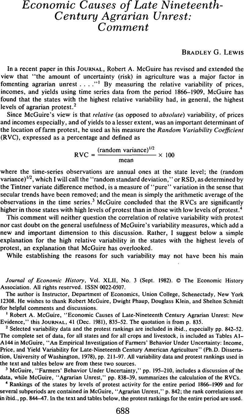
Economic Causes of Late Nineteenth-Century Agrarian Unrest: Comment
Published online by Cambridge University Press: 03 March 2009
Abstract

- Type
- Notes and Discussion
- Information
- Copyright
- Copyright © The Economic History Association 1982
References
1 McGuire, Robert A., “Economic Causes of Late-Nineteenth Century Agrarian Unrest: New Evidence,” this JOURNAL, 41 (12 1981), 835–52. The quotation is from p. 835.Google Scholar
2 Selected variability data and the protest rankings are included in ibid., especially pp. 842–52. The complete set of data, for all states and for all crops and livestock, is included as Tables Al–A144 in McGuire, , “An Empirical Investigation of Farmers' Behavior Under Uncertainty: Income, Price, and Yield Variability for Late-Nineteenth Century American Agriculture” (Ph.D. Dissertation, University of Washington, 1978), pp. 211–97. All variability data and protest rankings used in the text and tables below are from these two sources.Google Scholar
3 McGuire, “Farmers' Behavior Under Uncertainty,” pp. 195–210, includes a discussion of the data, while McGuire, “Agrarian Unrest,” pp. 838–39, summarizes the calculation of the RVCs.Google Scholar
4 Rankings of the states by levels of protest activity for the entire period 1866–1909 and for several subperiods are contained in McGuire, “Agrarian Unrest,” p. 842;Google Scholar the rank correlations are in ibid., pp. 844–47. In the text and tables below, the protest rankings for the entire period are used.
5 Ibid., p. 837.
6 Ibid., p. 838.
7 The term “enforced” in this context does not imply that the railroads acted as a cartel, but simply that the extensive network limited the size and direction of any price.differentials between any two locations.Google Scholar
8 See Table 1 below.Google Scholar
9 Prices of nontraded products that are good substitutes for traded ones could also show the same pattern.Google Scholar
10 An examination of mean yields for all seven crops included in the analysis below shows no such consistent pattern, although for some crops the highest yields are in the Group 2 states (Illinois, Iowa, Missouri, and Wisconsin).Google Scholar
11 McGuire, “Agrarian Unrest,” p. 838.Google Scholar
12 McGuire uses corn, wheat, oats, and in some cases, hay; see ibid., pp. 844–47. These are surely the most important crops, but potatoes, barley, and rye were grown in all 14 states and were important locally in some cases.
13 Ibid., p. 850.
14 Ibid., p. 848.
15 While shipments were made to other cities for export, New York City was the country's largest port and, with the possible exception of Chicago, its most important railroad terminus. Accordingly, distance from New York City is used as an estimate of the distance to eastern markets.Google Scholar
16 The distances were determined by averaging the distances on the major rail routes from state capitals to New York City. Route information was obtained from a 1926 railroad guide (National Railway Publication Company, Official Guide of the Railways and Steamship Lines of the United States, Porto Rico, Canada, Mexico, and Cuba, February 1926.)Google Scholar While this guide is for a later year than the period studied, it is unlikely that the use of averages obtained from it poses any difficulty: the major routes in the Northeast and Midwest were established during the late 1800s or earlier, and most construction after that time either duplicated existing routes or added branch lines. Moreover, to the extent that additional routes were added during the period, an arbitrary choice of the system at some intermediate date would be no more accurate for the entire period, either. In most cases the average was based on from two to five separate routes to New York City. The distances on competing routes did not differ by more than 10 percent except in Indiana (12 percent) and Ohio (20 percent).
17 The Spearman rank-order correlation coefficient for rankings by rail distance to New York and by protest levels is 0.961, significant at the 99.95 percent level.Google Scholar
18 For example, the RVC for corn for Kansas, the highest state, is 49.08 percent, while that for New York, the lowest, is 9.24 percent. See McGuire, “Agrarian Unrest,” p. 850.Google Scholar
19 For the weighted averages, production figures were obtained from U.S., Department of Commerce, Bureau of the Census, Fourteenth Census of the United States: 1920, vol. 5, Agriculture, pp. 739, 745, 752, 756, 760, 809, 813. In calculating both the weighted and unweighted averages, the author used a table of all the RSDs, available on request.Google Scholar
20 The Spearman rank-order correlation coefficients for such a small number of observations (n = 4) will only be significant above the 90 percent level if the coefficient is 1.000, i.e., if the ranks of the RSDs are exactly the same as the ranks by protest levels.Google Scholar
21 For example, North Dakota has the lowest RSDs for oats and potatoes, and Minnesota the lowest for corn.Google Scholar
22 In analyzing these measures of variability, the author prepared detailed tables for all crops, which include the rail distance, RVCs for incomes and prices, RSDs for prices and yields, and mean prices, incomes, and yields. These tables are available on request.Google Scholar
23 The Spearman coefficients were calculated using a standard correction procedure for ties to prevent biasing the significance levels upward. See, for example, Siegel, Sidney, Nonparametric Statistics for the Behavioral Sciences (New York, 1956), pp. 206–10.Google Scholar
24 For the regression analysis the state of New Jersey, the only Middle Atlantic or Midwest state excluded from the analysis of protest, was included; it seems clearly to have been a part of the same open economy.Google Scholar
25 If hay and corn are good substitutes, for instance, and if both could readily be raised on the same land, it would not be surprising to see similar price patterns across space. Also, despite its bulkiness, some hay was shipped to distant points. See Bogue, Allan G., From Prairie to Corn Belt (Chicago, 1963), pp. 143, 239.Google Scholar
26 Prices were test checked to those reported in U.S. Department of Agriculture, Bureau of Agricultural Economics, Prices of Farm Products Received by Producers. 2. The North Central States, Statistical Bulletin No. 15 (Washington, D.C., 1927), which is the original source of the data.Google Scholar
27 See U.S. Senate, Committee on Finance, 52nd Congress, Wholesale Prices, Wages, and Transportation. Report by Mr. Aldrich, Report 1394 (Washington, D.C., 1893); for transportation rates see vol. 1, pp. 516–22, 554, 648; for New York City prices see vol. 2, pp. 2, 7–8, 32–3, 35–36, 62–64.Google Scholar
28 This would not apply to yield variability, which of course could be a separate and important source of uncertainty.Google Scholar
29 If rates paid by shippers in some states were substantially higher than in others because of price discrimination, we would expect to see different slope coefficients or lower R2s, or both, in the regressions. Note that the price series measures farmgate prices.Google Scholar
30 It is a commonplace in financial theory that the holders of assets must typically be compensated for the systematic, but not the unsystematic, risk that they bear. See for example Weston, J. Fred and Brigham, Eugene F., Managerial Finance, 7th ed. (Hinsdale, Illinois, 1981), chaps. 5, 14.Google Scholar


