


1. Introduction
The purpose of this paper is to examine whether the expectation of having to provide care for aging parents may be a major factor contributing to the current low fertility rate in Japan. In so doing, this paper provides a link between the combination of a low fertility rate and an aging population that have become major concerns for many developed countries. Most of the countries in the Organization for Economic Cooperation and Development (OECD) have shown significant drops in their fertility rates since 1970 [OECD (2014)], and at the same time, life expectancy has risen due to improvements in medicine. Subsequently, their populations have been aging rapidly. An aging population challenges the maintenance of a pay-as-you-go pension system and also raises concerns that there may be a shortage of labor supply. These concerns raise policy interest in how we can increase the fertility rate.
The Japanese total fertility rate hit a minimum of 1.26 in 2005, and although recent statistics indicate a slight recovery in the fertility rate to 1.43 in 2017, the absolute number of births continues to decrease [Ministry of Health, Labour and Social Welfare (MHLSW) (2018b)]. Over the past three decades, the proportion of childless couples in Japan has more than doubled, and the proportion of couples with more than two children has shrunk (see Table 1).
Table 1. Number of children born to couples with a marriage duration of 15–19 years
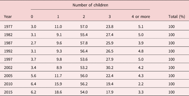
Note: For each year, the figures shown are the percentage of first-marriage couples who have been married for 15–19 years (excluding couples who did not state the number of their children) in each group.
Source: National Institute of Population and Social Security Research (IPSS) (2017).
Recently, the Japanese government has attempted to increase the availability of childcare to boost fertility [see, e.g., Nagase (Reference Nagase2018)]. Numerous empirical studies for different countries have examined the effects of fiscal instruments which aim to boost female employment and fertility. Some examine the impact of cash benefits on fertility [Kearney (Reference Kearney2004), Milligan (Reference Milligan2005), Björklund (Reference Björklund2006), Haan and Wrohlichc (Reference Haan and Wrohlichc2011), Cohen et al. (Reference Cohen, Dehejia and Romanov2013), Palermo et al. (Reference Palermo, Handa, Peterman, Prencipe and Seidenfeld2016)], whereas others examine the effects of the cost and availability of childcare on fertility [Blau and Robins (Reference Blau and Robins1989), Del Boca (Reference Del Boca2002), Mörk et al. (Reference Mörk, Sjögren and Svaleryd2013), Nagase (Reference Nagase2018)]. However, the empirical evidence on the effects of such policy measures is mixed [see Gauthier and Bartova (Reference Gauthier, Bartova, Shockly, Shen and Johnson2018) for a recent survey related to the impact of leave provisions]. Although providing cash benefits, reducing the cost of childcare, and/or increasing the availability of childcare and childcare leave may be important factors to increase fertility, this paper will examine this issue from a different perspective, that is, it examines whether the expectation of having to look after parents in the future has any effects on a couple's fertility.
One phenomenon that has attracted attention recently is the “sandwich family” which refers to couples who are trying simultaneously to raise young children, to take care of aging parents and to work full time [see Fox (Reference Fox and Roloff2012)]. This paper considers the possibility that couples who expect that they will have to care for their aged parents in the future may reduce the number of children they plan to have. We argue that these couples do so because they try to avoid or reduce the possibility of a sandwich generation where the couples have to look after both their parent(s) and their dependent children at the same time. Japan's Employment Status Survey provides a picture of the actual impact of caring for family members on household activities [Ministry of Health, Labour and Social Welfare (2012)]. During the 5-year period from October 2007 to September 2012, about 487,000 Japanese workers quit their jobs to provide care to an aged or sick family member, that is, nearly 100,000 workers per year. About 80% of these workers are female. Notwithstanding these results, Oshio and Usui (Reference Oshio and Usui2017) find that providing informal parental care has little impact on the female employment of women aged 50–59, that is, whether these women work or not. In contrast, Shimizutani et al. (Reference Shimizutani, Suzuki and Noguchi2008) find that the introduction of the Long-term Care Insurance Scheme in 2000 had significant positive effects on employment and hours worked due to the reduction in caring responsibilities.
At the time it was founded in 2000, Japan's Long-term Care Insurance Scheme was a public universal long-term care insurance system initially financed by a levy on all individuals aged 40 and over. The benefits provided by the scheme depend on the needs of the individual, and the care recipient had to pay for a part of the cost of the services being provided [see Campbell et al. (Reference Campbell, Ikegami and Gibson2010) for further details]. It is important to note that this paper examines data prior to the introduction of the Long-term Care Insurance Scheme in 2000, so that the responsibility for looking after aged parents was primarily on the shoulders of family members rather than private institutions. Table 2 reports who takes care of a family member when that member is in need of care after the Long-term Care Insurance Scheme was introduced. More than 95% of such frail family members are aged 65 years or older [MHLSW (2017)]. According to Table 2, in 2016, a little less than 60% of family care providers live with the family member when that family member is in need of care. In 2016, even with the Long-term Care Insurance Scheme in place just over 70% of the care providers are cohabiting and non-cohabiting family members, and only 13% of them are private care providers!

The cost of private care is very expensive. It is estimated that in 2018 before social security payments, an individual who receives private care spends on average around 170,000 Japanese yen [US$1,550 ($1 = 110 yen)] per month for these services [MHLSW (2018a)]. In 2015, the Nihon Keizai Shinbun reported that the average duration of aged parental care was 4 years and 11 months, and the average monthly out of pocket cost for aged parental care was 69,000 Japanese yenFootnote 1 which was about 16% of the average monthly household income of 430,000 yen at the time. Thus, on average, the total cost of care is 4 million yen for 4 years and 11 months. If a couple decides to put a parent in a nursing home, then the monthly nursing home fees range from 150,000 to 300,000 yen excluding one-off entry fees.
The long-term decline in the fertility rate in Japan means that over time aged parents have to be looked after by fewer children, and possibly for longer periods of time due to the rise in life expectancy. For the children who are potential care providers, this means that the cost of future care of their aged parents has increased substantially over time. Departures from the workforce or reductions in their market labor supply due to the provision of family care lead to a reduction in an individual's lifetime income, and this in turn potentially reduces their demand for children.
There is of course a literature that links the available social security package to a couple and the number of children they have [e.g., Boldrin and Jones (Reference Boldrin and Jones2002) and Boldrin et al. (Reference Boldrin, De Nardi and Jones2015)], however, our search of the literature suggests that the only other paper that discusses a direct link between caring for the aged and child rearing is Sakata and McKenzie (Reference Sakata and McKenzie2014). Their focus is on the connection between the expected burden associated with caring for parents and the quality of children, rather than the quantity of children that is analyzed here. Sakata and McKenzie's (Reference Sakata and McKenzie2014) proxy variable for the expected future burden of caring for parents is based solely on the number of parents and parents in law who are alive at the time of the couple's marriage divided by the total number of siblings of the husband and wife including themselves. In contrast, in this paper, an estimate of the probability that a couple will look after their parents or parents-in-law is obtained from a model estimated using past data and the characteristics of the couple at the time of their marriage. There is evidence that the probability of having to look after parents reduces the probability of having any children.
Forward looking behavior by agents is strongly emphasized in economics. However, considering young adults' family planning decisions, there is an issue about how far into the future agents look. In our data set, the average ages that men and women married were 27.7 and 24.9 years old, respectively.Footnote 2 For their parents who were living at the time of their marriage but who had died by the time of the survey, the average time from the marriage to their death was 15.2 years and 20.5 years for the husband's father and mother, and 16.7 years and 21.9 years for the wife's father and mother, respectively. Assuming that caring occurs immediately before the death of the parent, this means that if they engage in caring, husbands and wives are on average likely to be in their 40s. It could be suggested that events expected to happen 15–20 years in the future have little impact on current behavior, but there is evidence to suggest these events can have an impact. According to the Public Opinion Poll on Old Age Care (Koureisha kaigo ni kan suru yoron chosa)Footnote 3 conducted by the Japanese Cabinet Office in 2003, 67% and 69% of males and females in their 20s report that they have some anxieties about family members requiring long-term care in the future. According to the Survey on the Financial Asset Choice of Households (Kakei ni okeru kinyu shisan sentaku ni kan suru chosa) 2001Footnote 4 conducted by Japanese Ministry of Internal Affairs and Communications (2017), 8.6% and 23.1% of households headed by someone in their 20s and 30s, respectively, reported that some of their saving was motivated by preparing for their own life in old age. For young Americans aged 22–35, Knoll et al. (Reference Knoll, Tamborini and Whitman2012) show that a significant minority have individual retirement accounts. Murata (Reference Murata2003) suggests that uncertainty about public pension system payments has an impact on the current wealth holdings of young Japanese households (those with a husband aged between 23 and 45). Thus, there is some evidence to suggest that young adults do look quite far ahead into the future to make their intertemporal decisions related to saving.
In this paper, we estimate how the expectation of having to provide care for aging parents affects a couple's current fertility using a two-stage model. The first stage of a couple's family planning decision is a logit model which examines the decision of whether or not a couple have any children, and then in the second stage a Poisson model is applied to explain the number of children a couple has conditional on the couple having at least one child. Our findings show that there are strong generational effects, and that for the post-war cohort, an increase in the probability of having to look after a parent increases the probability of a couple being childless.
The rest of this paper consists of four sections. Section 2 discusses the burden hypothesis and section 2 introduces the empirical model, section 3 introduces the empirical model, whereas section 4 describes the data. Section 5 reports the estimation results and discusses their implications. Section 6 contains a brief conclusion.
2. Theoretical model
The neoclassical economic theory of fertility contends that the decision to have a child is a function of the costs and benefits of children subject to an income constraint and an individual's preference for children. Under such a utility maximization process, the neoclassical economic theory of fertility predicts that any reduction in the cost of having children or any increase in income induces an increase in the demand for children [Becker (Reference Becker1993)]. If an individual has to leave the labor force or reduce his/her labor supply so as to care for frail and aging parents, the individual's lifetime income will be reduced dramatically. In addition, if the cost of (an)other good(s) namely, the cost of future care for aged parents, increases, individuals may have to compromise their consumption on children. We argue that any increase in the cost of future care for aged parents will reduce the demand for children. Thus, an increase in the future burden of caring for frail and aging parents reduces the demand for children.
Here, we use a simple model to develop some of the points argued by Becker (Reference Becker1993). Suppose we have a consumer who lives for two periods. In the first period, the consumer (generation 2) has children (generation 3) and provides assistance to his/her parents (generation 1).Footnote 5 In the second period, the generation 2 consumer receives assistance from his/her children. Suppose that the generation 2 consumer's consumption in period j is denoted by C j, the number of children is given by N, and that the generation 2 consumer's utility function is given by

where α > 0 and β > 0, and the consumer's budget constraint is assumed to be

where r is the interest rate, γ > 0 is the cost of having each child, the financial assistance provided by the generation 2 consumer to the consumer's parents in the first period is denoted by A 21, the financial assistance provided by the consumer's children to the consumer in the second period is denoted by A 32, and the net present value of the total income earned by the generation 2 consumer in the first and second periods is given by Y. It is easy to show that if the generation 2 consumer's choice variables are C 1, C 2, and N, then the solution for N to maximize the utility function in (1) subject to the budget constraint in (2) is given by

so that

The result in (4) is not surprising given the form of the utility function in (1), as it is easy to show that consumption in both periods and children are “normal” goods, so that demand for these goods will increase if the total income of the generation 2 consumer increases. In this case, the available resources for the generation 2 consumer are Y + A 32/(1 + r) − A 21, so an increase in expenditure on the parents in generation 1 naturally leads to a fall in the available resources for the generation 2 consumer, lower consumption in both periods 1 and 2, and a lower number of children in generation 3.Footnote 6
The expected cost to a couple today of looking after a parent in the future has several important dimensions including: the level of care that the parent requires; the duration of time that the parent requires care; the actual cost (economic and psychological) of looking after the parent; how many years into the future it will be that the parent is expected to begin to require care; and the couple's expectation of the probability that they will be caring for the parent. The actual cost of looking after the parent may depend on factors such as the parent's customary standard of living which might depend on socio-economic background; location; and the income of the child (since cost is relative to income).Footnote 7, Footnote 8 Using JSTAR data from 2007, 2008, and 2009, Ibuka and Ohtsu (Reference Ibuka and Ohtsu2020) provide some evidence for Japan on how the socioeconomic status (SES) of the children affects the probability that they look after their parents or parents in law. Although finding that for those households in higher SES categories there is a higher probability of providing care, Ibuka and Ohtsu (Reference Ibuka and Ohtsu2020) do not find any systematic connection between particular SES measures and the care probabilities. Of all the dimensions of the expected cost to a couple today of looking after a parent in the future, given the data available in the surveys we are using we focus on the probability that the child will care for a parent in the future.
3. Empirical model
We first discuss how we model the impact of the probability of having to look after a parent on a woman's fertility (section 3.1), and then we consider the question of how to estimate the probability that a person has to look after a parent or a parent in law (section 3.2).
3.1 Estimating the effects of the probability to look after a parent on fertility
This section discusses modeling a couple's decision relating to their family size. It is assumed that couples decide on their family size at the time of their marriage.Footnote 9 To be specific, the dependent variable to be explained is the number of children born to a woman who is aged 45 years or older as we assume that women of this age have completed their childbearing activities. The focus of the analysis is whether the estimated probability of the couple being the primary care provider for at least one parent or parent in law, P i, has any effects on the wife's fertility.
As the existing literature [e.g., Melkersson and Rooth (Reference Melkersson and Rooth2000) and Santos Silva and Covas (Reference Santos Silva and Covas2000)] has argued, there may be a significant difference between childless couples and couples with at least one child. Both Melkersson and Rooth (Reference Melkersson and Rooth2000) and Santos Silva and Covas (Reference Santos Silva and Covas2000) argue that the outcome of zero children may result from two distinct sources: a couple choosing to have no children or a couple being physically unable to have children at all, whereas the outcome of one or more children is just a result of a couple's choice. Given this difference between childless couples and couples with children, one way of modeling this is to use a Poisson logit hurdle model. The first-stage model is a logit model that examines the decision of whether to have a child or not, and in the second stage for couples who decide to have children a standard Poisson regression model is used to explain the number of children they have. Another reason for preferring the Poisson hurdle model is that the Poisson model which assumes that the mean and the variance of the number of children are the same cannot explain the observed under-dispersion in the number of children.
If the number of children that couple i has is denoted by yi, then assuming a Poisson hurdle model means the probability of having 0, 1, …, N children is given by [see Winkelmann (Reference Winkelmann2003) and Cameron and Trivedi (Reference Cameron and Trivedi2013)]:


where wi is given by a logistic function, namely,$\;w_i = 1/( {1 + \exp ( {x_i^{\prime} \gamma } ) } )$ and $\lambda _i = \exp ( {x_i^{\prime} \beta } )$
 .Footnote 10 In this model, $E( {y_i{\rm \vert }y_i > 0} ) = 1 + {\rm exp}( {x_i^{\prime} \beta } )$
 and E(y i > 0) = 1 − w i, so that for variables that are continuous $\partial E( {y_i{\rm \vert }y_i > 0} ) /\delta x_i = \exp ( {x_i^{\prime} \beta } ) \beta$
 , ∂E(y i > 0)/δx i = w i(1 − w i)γ, and $\partial E( {y_i} ) /\partial x_i = \exp ( {x_i^{\prime} \beta } ) \beta \;( {1-w_i} ) \lambda _i^j$
 . It should be noted that the standard Poisson model and this Poisson hurdle model are non-nested models, so that one way to choose between them is to use an information criterion like the Akaike information criterion (AIC) or the Bayesian information criterion (BIC).
If we think of the bivariate choice problem of having no children or some children, the model in equations (5a) and (5b) will imply this choice is determined by a logit model with Prob(y i = 0|x i) = w i and obviously Prob(y i > 0|x i) = 1 − w i. In fact, as McDowell (Reference McDowell2003) indicates an equivalent way to estimating the model in equations (5a) and (5b) by maximum likelihood is to first estimate a logit model with Prob(y i = 0|x i) = w i and Prob(y i > 0|x i) = 1 − w i, and then for y i > 0 to estimate a Poisson model.
The vector of control variables, xi, includes the probability of the couple looking after their parents and/or parents-in-law, P i, that is discussed in detail in section 3.2, and other control variables such as the husband's age at the time of his marriage, the wife's age at the time of her marriage, the husband's education level, the wife's education level, an urban dummy, and seven regional dummies. In addition, we include a 0–1 dummy variable which takes the value 1 if husband is an only child and 0 otherwise to control for some of the effects of being the eldest son.Footnote 11 The a priori expectation is that a higher probability of the couple looking after their parents and/or parents-in-law will tend to reduce the number of children the couple has.
3.2 Estimating the probability of having to look after a parent
As indicated in Table 2, in Japan the primary care providers for frail aging parents are typically other family members rather than private care providers. If a parent or parent-in-law has died before the survey, the 1998 National Family Research of Japan (NFRJ98) survey contains information on whether the respondent reports that he/she was the primary care provider for that person before they died. For each deceased father, mother, father-in-law, or mother-in-law, the NFRJ98 survey asks respondents whether the relevant parent or parent-in-law required care for a period before they died, and if the answer is yes, respondents are then asked “(t)o what extent were you involved in caregiving and nursing?” The respondent picks an answer from one of the following five choices: (1) I was the primary person involved in care providing and nursing; (2) I was involved, though not as the primary care provider; (3) I was somewhat involved; (4) I was not much involved; and (5) I had very little opportunity to be involved because of the person's sudden death. Based on cases where the relevant parent or parent-in-law had already died by the time of the survey, Table 3 provides information on whether the parent or parent-in-law required care, and when care was required who provided what level of care to whom.
Table 3. Who provides how much care to whom?
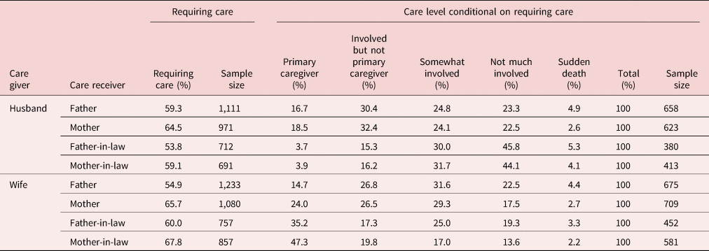
Notes: (1) The columns labeled “Requiring care” report the percentage of care givers who reported that the relevant care receiver required care before his/her death and the sample size on which this calculation is based. The columns labeled “Care level conditional on requiring care” report the percentage of respondents who said they provided a particular level of care for a specified parent or parent-in-law conditional on having reported that the specified parent or parent-in-law required care for a period of time before his/her death. In both cases, the information is only available if the relevant parent or parent-in-law has died by the time of the survey, and in the case of the “Care level,” the care giver reported that the relevant parent or parent-in-law required care for a period before his or her death. This is one of the important reasons for differences in the sample sizes for identical care givers.
(2) This table contains estimates of whether care was required for the two types of caregivers and four types of care receivers based on respondents' answers to questions 32, 33, 34, and 35 for his/her father, mother, father-in-law, and mother-in-law, respectively, on the 1998 NFRJ survey. This table contains estimates of the care level provided by the two types of caregivers and four types of care receivers based on respondents' answers to supplementary questions 1 for questions 32, 33, 34, and 35 for his/her father, mother, father-in-law, and mother-in-law, respectively, on the 1998 NFRJ survey. It should be noted that these questions are only asked on the 1998 NFRJ survey.
Source: Computed from the 1998 NFRJ survey.
Perhaps the most surprising finding in Table 3 compared to the conventional wisdom is that for their own parents both the husband and wife report that they are just as likely to be the primary care provider. For example, 16.7% of husbands report they were the primary carers for their fathers. On the contrary, 14.7% of wives were the primary carers for their fathers. Wives are more likely to be the primary carers for their own mothers than their husbands (24%), but still 18.5% of husbands were the primary carers for their own mothers. In the Japanese context, it is not surprising to find that husbands do not look after their in-laws as the primary care provider (less than 4% for in-laws), but their wives do and they are more likely to do so than for the case of the wife looking after her own parents! In total, 35.2% of wives were the primary carers for their father-in-law and 47.3% of them were the primary carers for their mother-in-law. The proportions of wives who became the prime carers for their parent-in-laws are much higher than that of their own parents. In the case of wives, there is a strong cultural expectation that they will be strongly involved in caring for their husbands' parents.
In order to measure the future burden of caring for aged parents, we construct a probability of having to look after a parent or parent-in-law in the future. For the ith couple, let p ijk be the probability of individual j in couple i looking after parent k where j denotes either the husband (h) or wife (w) and k refers to the husband's (h) or wife's (w) parent(s). For example, for the husband of the ith couple, the probability of looking after his own parent(s) (husband's parents) is denoted by p ihh and the probability of looking after his parent(s)-in-law (wife's parent) is denoted by p ihw.
In order to estimate the probability of looking after a parent in the future, the information in NFRJ98 is more appropriate than the information on whether the respondent is currently involved in caregiving and nursing a parent as many of the respondents do not yet have aging frail parents. Another advantage of this information is that when computing the probability of looking after a parent we can take account of those cases where a parent's death was sudden and the respondent did not have to provide any care to that parent.
Denoting the husband and wife by h and w, respectively, we construct four 0–1 dummy variables care ijk (j = h, w, k = h, w) which take the value one if the ith respondent was the husband (j = h) or wife (j = w) and “the primary person involved in care providing and nursing” for k's parents where k denotes the husband (h) or the wife (w), and 0 otherwise, and denote the associated probability of care ijk = 1 by p ijk, then the following probit model is used to model p ijk and explain the two outcomes for care ijk, for each value of j and k, namely,Footnote 12, Footnote 13

where η ijk is a normally, identically and independently distributed random variable with expected value zero and variance 1, and Njk is the available sample size for the relevant combination of j and k.
For CARE ijk, the following four models are assumed:


where $siblings\_ j_i$ is the number of js siblings [husband (j = h) or wife (j = w)],Footnote 14 $one\_parent\_ j_i$
 is a 0–1 dummy variable which takes the value one if one of js parents is already deceased at the time of his/her marriage, and 0 otherwise [husband (j = h) or wife (j = w)], $birth\_year\_ j_i$
 is the year of the birth of individual j [husband (j = h) or wife (j = w)], and $educ\_ j_i$
 is the years of education for individual j [husband (j = h) or wife (j = w)]. As Table 2 indicates, in around 25% of all cases a cohabiting spouse is the care provider, so the variable $one\_parent\_ j_i$
 highlights the fact that if one of the parents is already deceased at the time of a couple's marriage, the probability of having to look after a parent should increase. $birth\_year\_ j_i$
 is included to control for cohort effects, and $educ\_ j_i$
 is used as a proxy for income. Although parental income at the time of marriage may be an important predictor of the probability of their children having to provide future care, such information is not available in our data set.Footnote 15 When estimating equations (7)–(10), the values of the variables at the time of the couple's marriage are used. Similarly, when the probability of looking after a parent is calculated the explanatory variables used in equations (7)–(10) are measured at the time of the couple's marriage.
In equations (7)–(10), one key issue is the sign of β i1, i = 1, 2, 3, 4, that is, the impact of the number of siblings. There are a number of possibilities depending on what assumptions are made. If we assume that the couple in question is completely selfish, then they will not care about the provision of care for their parents or for their parents-in-law by themselves or by their siblings, and so the number of siblings that a couple has should be irrelevant, that is, β i1 = 0, i = 1, 2, 3, 4 [the other coefficients in equations (7)–(10) would also be expected to be zero]. If care provision is driven by a “warm glow” motivation, then the couple may provide care to their parents (or parents-in-law) depending on the strength of the warm glow motivation. In this case, the provision or lack of provision of care by siblings is again irrelevant. One simple story for why β i1 > 0 is that if there is only one primary care provider, then on a probabilistic basis with more siblings, the likelihood of being the primary care provider can be expected to be smaller. A more sophisticated story would assume that the couple and the couple's siblings are all altruistic with respect to their parents (and parents-in-law), so that the provision of care for their parents (parents-in-law) by them and their siblings can be viewed as being a version of a public goods game. Assuming that both parents and children only care about the total contribution made by the children, increases in the number of siblings will reduce the individual contributions made to the first-generation parents by each second-generation sibling.Footnote 16
Once estimates of the parameters of equations (7)–(10) have been obtained, using these estimated coefficients and a different sample of all the available married men and women, respectively, including those who yet to experience the death of their parents or parents-in-law in the 1998 and 2008 NFRJ surveys estimates of p ihh and p ihw, and p iww and p iwh can be obtained by inserting the values of explanatory variables and estimated parameters into equations (6)–(10).
Caregiving and nursing of a frail parent should be seen as the joint product of couple. For example, a husband may not be the primary care provider if he is the breadwinner of the household, but his wife can be the primary care provider. Thus, the probability of the couple having to look after at least one of their parents or parents-in-law as a couple, Pi, can be written asFootnote 17:

Here, (1 − p ihh) is the husband's probability of not becoming the primary care provider for his parents. Therefore, (1 − p ihh) × (1 − p ihw) × (1 − p iww) × (1 − p iwh) is the probability that neither the husband nor the wife are the primary care provider for any of their parents or parents-in-law.
4. Data
The data used in this paper are drawn from two repeated cross-section surveys, the 1998 and 2008 National Family Research of Japan (NFRJ, Kazoku nitsuiteno Zenkoku Chousa) surveys.Footnote 18 These surveys are conducted by the Japan Society for Family Sociology, and the data are archived in the Social Science and the Social Science Japan Data Archive, Information Center for Social Science Research on Japan, Institute of Social Science, The University of Tokyo. The surveys were conducted by the drop-off-pick-up method. In the 1998 survey, 10,500 individuals who were aged between 28 and 77 as of December 1998 were surveyed with a response rate of 66.52% (6,985 responses). In the 2008 survey, 9,400 individuals who were aged between 28 and 72 as of December 2008 were surveyed, and the response rate was 55.35% (5,203 responses). The properties of the 1998 and 2008 NFRJ data sets, including their representativeness, are discussed in Japan Society of Family Sociology (2000, 2010), respectively.Footnote 19
In our fertility analysis, the two surveys are pooled and a survey year dummy is added [see Roberts and Binder (Reference Roberts and Binder2009)]. One of the advantages of using the NFRJ data sets is that they contain rich information on parents and siblings. Here, information on whether the married respondent's parents and parents-in-law are alive at the time of the respondent's marriage is used. Furthermore, information on the number of siblings the respondent has and the number of siblings for his/her spouse has is also used.
4.1 Sample selection
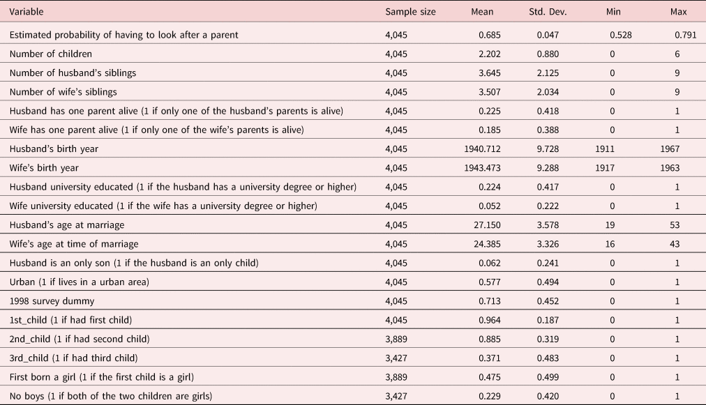
We estimate our models explaining the number of children for households that satisfy the following eight criteria. First, couples where the wife's age is 45 years or older in order to focus on those women who have completed child bearing. Second, we focus on married respondents where the husband's age at the time of the marriage is 18 years old or older and the wife's age at the time of the marriage is 16 years old or older. This is because the Japanese legal age for marriage is 18 for men and 16 for women. Third, we only use respondents who are currently married and who have never been divorced or widowed. Divorcees or widows may have children from their previous marriage, but the NFRJ surveys do not contain information on their previous marriages. Fourth, we also exclude an observation if the wife's age at her marriage was 45 or older as she is unlikely to have any child. Fifth, we drop observations which report a deceased child as this can have an impact on later fertility decisions. Sixth, in order to control for outliers, observations where there are 10 or more siblings (99% quantile) are excluded. Seventh, we exclude all marriages from 1997 onward to eliminate the actual or anticipated effects of the Long-term Care Insurance Act (Kaigo Hoken Ho) which passed into law in December 1997 and came into effect on April 1, 2000. Eighth, we exclude all observations which do not contain all the information on all the variables required for estimating the relevant model. After imposing these selection criteria, 4,045 observations remain. Descriptive statistics for this sample are summarized in Table 4. Using the mean (2.2) and the standard deviation of the number of children (0.88) reported in Table 4, we can see that the variance of this variable (0.77) is just one-third of the size of the mean, a strong indicator of under-dispersion.
Table 4. Descriptive statistics for the samples used to estimate the logit, Poisson, and Poisson-logit hurdle models
5. Results and discussion
All results reported are obtained using STATA Version 16 [StataCorp. (2019)]. Table 5 reports the results of estimating equation (6) with each of (7), (8), (9) and (10) for two cases, one where the number of siblings is the only explanatory variable, and the other which also includes the birth year of the carer, a dummy for the carer having a university education, and a dummy for one of the relevant parents being dead. The sibling variables all have negative estimated coefficients and the variables are statistically significant in the cases of a husband looking after his parents in law [(5.3) and (5.4)] and a wife looking after her own parents [(5.5) and (5.6)] and her parents in law [(5.7) and (5.8)], that is, as the number of siblings increases the probability of being the primary care provider falls. In the equations analyzing the factors affecting a husband being the primary care giver for his parents [equations (5.1) and (5.2)] nothing is statistically significant. This suggests that it is rather hard to systematically forecast whether or not a husband will look after his own parents. For the other equations, none of the variables apart from the number of siblings are individually or jointly significant.
Table 5. Probability to look after a parent or parent-in-law
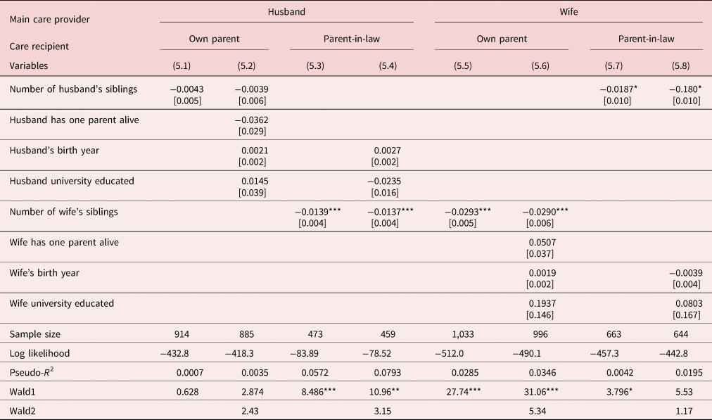
Notes: (1) Each equation is estimated as a probit model where the dependent variable takes the value of 1 if husband (or wife) was the main care provider for the particular care receiver, and 0 otherwise. This variable is not conditioned on whether the care recipient having received care before his/her death.
(2) For each variable, marginal effects are reported, and the figures in brackets are robust standard errors.
(3) The statistical significance of variables or Wald tests at the 1%, 5%, and 10% significance levels are denoted by ***, **, and *, respectively.
(4) All equations include a constant term whose estimated coefficient is not reported.
(5) Wald1 reports the value of a Wald test for the null hypothesis that all the coefficients (excluding the constant) are jointly zero.
(6) Wald2 reports the value of a Wald test for the null hypothesis that all the coefficients except for the constant and the coefficient for the number of siblings are jointly zero.
(7) The two parent-in-law equations, equations (5.4) and (5.8), do not contain the one parent dummy because it was a perfect predictor.
Given the results in Table 5, we use the parameter estimates from the models that only contain the number of siblings [(5.1), (5.3), (5.5), and (5.7)], to compute the probability of a married couple having to look after at least one parent, P i. Since P i is a generated regressor, the standard errors in any model that uses this generated regressor will, in general, not be computed appropriately [see Newey and McFadden (Reference Newey, McFadden, Engle and McFadden1994)], so bootstrapped standard errors based on 1,000 replications are reported.Footnote 20
It can be argued that there may be substantial generational differentials in fertility among the respondents.Footnote 21 Japanese society has undergone a huge transition during the World War II and the post-war period. Urbanization and the rise of the nuclear family can be expected to have huge impacts on family planning and the support families provide for frail aging parents. To account for possible cohort effects, the sample was divided into three groups according to the “generation” the husband belonged to: those husbands born before 1938; those husbands born between 1937 and 1947; and those husbands born after 1946.Footnote 22 We used this division to compare the post-war generation and previous generations, and at the same time, to maintain a sufficient sample size in each cohort.
5.1 Preliminary logit analysis
Before estimating the Poisson-logit hurdle model specified in equations (5a) and (5b), some preliminary logit analyses to show the difference between childless couples and couples with one or more children are conducted. Three logit models for the first birth, the second birth, and the third birth, respectively, are estimated. For the first birth case, the dependent variable is a 0–1 binary variable which takes the value 1 if the couple has at least one child and 0 otherwise. For the second (third) birth case, the dependent variable is a binary variable which takes the unity if the couple has at least two (three) children, and takes the value 0 if the couple has only one child (two children). Of course, the logit analysis for the first birth is part of the analysis involved in the Poisson-logit hurdle model. Moreover, as Wakabayashi and Kureishi (Reference Wakabayashi and Kureishi2011) indicate, there is evidence to suggest that a son preference exists among the older generation in Japan, so we include an additional variable to account for son preference in the models for second and third births. “First born a girl” is a dummy variable that takes the value 1 if the first child is a girl, and 0 if it is a boy. “No boys” is a dummy variable which takes the value unity if the first child and second child are both girls, and 0 otherwise. Son preference would be consistent with positive coefficients on the First born a girl and No boys in the models for second and third births, respectively.
The estimated results for the logit analyses for the first, second, and third births are summarized in Table 6. In addition to results for the full sample, this sample is divided into three sub-samples to try and account for cohort effects. For first births, the probability of having to look after at least one parent is significant and has a negative impact overall and for the post-war cohort born after 1946. This suggests that for the post-war cohort a couple with a high probability of looking after a parent in the future is more likely to be childless. On the contrary, for both second and births, the estimated coefficient on P i is not significant in any case. Thus, there appears to be some strong cohort effects. The post-war generation, born after 1946, is more likely to reduce the family size when they face a high probability of having to look after a parent. The results for the post-war cohort are consistent with the macro-data reported in Table 1. According to Table 1, there has been a significant increase in the proportion of couples that are childless, but the proportion of couples with two children has remained rather steady.
Table 6. Results of estimating logit models for each birth occurrence

Notes: (1) For each variable, marginal effects are reported, and the figures in brackets are bootstrapped standard errors based on 1,000 replications. The statistical significance of variables at the 1%, 5%, and 10% significance levels are denoted by ***, **, and *, respectively. All equations include a constant term whose estimated coefficient is not reported.
(2) Wald Test is a Wald test of the null hypothesis that all coefficients in the model (except for the constant) are jointly zero.
It is important to note that the empirical evidence suggests there is a son preference in Japan as the “First born a girl” dummy has a positive and significant coefficient for second births [equation (6.5)] and the “No boys” dummy has a positive and significant coefficient for third births [equations (6.9) and (6.10)]. However, the younger generation cohort (husband born after 1946) does not have a son preference as the coefficients on these variables tend to be insignificant for the younger cohorts. These results are consistent with Wakabayashi and Kureishi (Reference Wakabayashi and Kureishi2011).
5.2 Poisson-logit hurdle analysis
Before estimating a Poisson hurdle model, it is worth estimating a standard Poisson model. The results of estimating a Poisson model are reported in Table 7. Using all the observations, the probability of having to look after at least one parent has a positive, but insignificant estimated coefficient. When the sample is divided into the three cohort groups, the estimated coefficient on the probability of having to look after at least one parent is only significant in the case of the cohort born after 1946, and in this case it has a negative sign, that is, an increase in the probability of having to look after at least one parent reduces the number of children. This is consistent with the findings from Table 6. Later marriage ages for both husbands and wives tend to be associated with fewer children. However, it is worth noting that the deviance goodness-of-fit and the Pearson goodness-of-fit tests all indicate that the Poisson distribution is not a good choice to explain these data. In addition, the diagnostic tests for under-dispersion indicate the presence of a considerable amount of under-dispersion.
Table 7. Estimates of a Poisson model
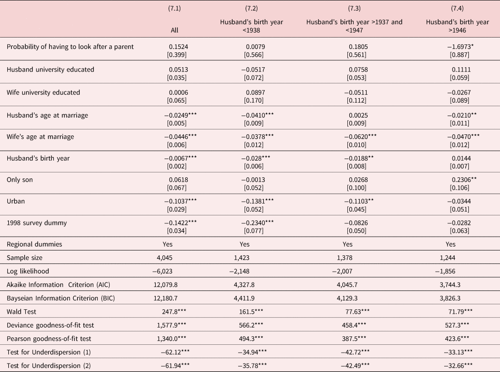
Notes: (1) The statistical significance of variables at the 1%, 5%, and 10% significance levels are denoted by ***, **, and *, respectively.
(2) The estimates of the constant terms are not reported.
(3) The figures in brackets are bootstrapped standard errors based on 1,000 replications.
(4) Wald Test is a Wald test of the null hypothesis that all coefficients in the model (except for the constant) are jointly zero.
(5) The deviance and Pearson goodness-of-fit tests are tests of goodness of fit. Significant values suggest the Poisson model is inappropriate.
(6) Test for Underdispersion (1) and (2) are t-tests based on Cameron and Trivedi's (Reference Cameron and Trivedi1990) equation (4.5) where the predicted expected value of the dependent variable and a constant are used as the explanatory variable, respectively. Negative values are indicative of underdispersion.
As discussed earlier, the difference between childless couples and couples with children may be significant, and one way of modeling this is to use a Poisson logit hurdle model. As McDowell (Reference McDowell2003) points out maximum likelihood estimates of the Poisson-logit hurdle model can be obtained by estimating a logit model for the no children or some children outcomes, and then estimating a Poisson model for the number of children conditional on there being one child. Since the results of the relevant logit models are reported in Table 6, Table 8 only reports the marginal effects obtained for estimating a Poisson model for the number of children conditional on there being one child. The AIC or the BIC reported in Table 8 are for the Poisson-logit hurdle model, and when compared with the models in Table 7 lead to a clear choice in all cases in favor of the Poisson hurdle models reported in Table 8. However, in none of these models does the probability of having to look after a parent or parent-in-law have a positive statistically significant. This is consistent with results reported for second and third births in Table 6. Later marrying by wives and in some cases for husbands lead to fewer children.
Table 8. Estimates of the Poisson portion of the Poisson-logit hurdle model
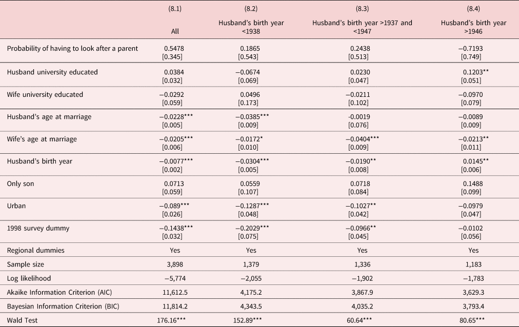
Notes: (1) This table reports the Poisson portion of the Poisson-logit hurdle model. The logit portions of these models are reported in Table 6. The log likelihoods, AICs and BICs reported in this table are for the Poisson-logit hurdle models as a whole not just for the Poisson portion of the model.
(2)The statistical significance of variables at the 1%, 5%, and 10% significance levels are denoted by ***, **, and *, respectively.
(3) The estimates of the constant term in the Poisson models are not reported.
(4) The figures in brackets are bootstrapped standard errors based on 1,000 replications.
(5) Wald test is a Wald test of the null hypothesis that all coefficients (except for the constant) in the Poisson model are jointly zero.
6. Concluding remarks
This paper examines whether the expectation of having to look after parents in the future affects current fertility. The main focus of research in this area has been on the effects of factors such as female labor force participation, childcare availability, and childcare benefits on fertility. In contrast, this paper proposes that the expectation of future care for aging parents may be another major factor contributing to the low fertility rate in Japan. As far as we know, no study has examined the effects of the future burden of aging parents on fertility. In this paper, a Poisson-logit hurdle model is used to examine this issue. The first-stage model is a logit model which examines the decision of whether to have a child or not, and in the second stage the number of children is explained using a Poisson model. The empirical evidence based on estimates of the logit Poisson hurdle model suggests that there are strong generational effects. In particular, for the post-war cohort, an increase in the probability of having to look after a parent increases the probability of couples being childless.
Under the Japanese Long-term Care Insurance Law (Kaigo hoken ho) of 1997, a Nursing Care Insurance system which aims to reduce the burden of aged care on families by introducing a compulsory national nursing care insurance levy, and using the revenue from that levy to fund nursing care for those requiring it began operation on April 1, 2000. Kan and Kajitani (Reference Kan and Kajitani2014) find that the introduction of the Public Nursing Care Insurance significantly reduced the time that wives devoted to nursing care. If the expectation of having to look after parents in the future affects current fertility, then as Kan and Kajitani (Reference Kan and Kajitani2014) find the introduction of long-term care benefits in 2000 should reduce some of the burden on families to care for their parents and possibly work to increase the fertility rate over the short- and long-term. The Japanese fertility rate has slightly increased since 2005 and casual empiricism might suggest that this results from this policy change. Our next research goal is to examine the impacts of the introduction of compulsory long-term care benefits scheme in 2000 on fertility.
The analysis in this paper has assumed that the age at which the husband and wife get married are not affected by the probability that they will have to look after their parents or parents-in-law. Given that women bear a disproportionate weight of the burden associated with caring for parents and parents-in-law, it is possible that women delay the age at which they marry or do not marry at all. Since the age at which the wife marries has (a) a statistically significant and negative effect on whether to have children or not, and (b) in the case where the couple decides to have children, this age also has in most cases a statistically significant negative effect on the expected number of children, considering this indirect channel for their impact of the probability of care could lead to an even stronger effect than is found in this paper.
One potential motive for parents to have children is that if the parents think about their own aged care in the future. In this case, there would seem to be an incentive to have more children, but for your own care it is not obvious whether it is better to have a small number of high quality children or a large number of lower quality children, or to choose to save for old age rather than having children.
Supplementary material
The supplementary material for this article can be found at https://doi.org/10.1017/dem.2020.35.
Acknowledgements
Both authors wish to thank Murat Iyigun (Associate Editor), an anonymous referee, Shinya Kajitani, Philip McKenzie, Ai Takeuchi, Emiko Usui, and the participants at the Tenth Annual Conference of the Asian-Pacific Economic Association, the 79th International Atlantic Economic Conference, an Autumn Meeting of Japanese Economic Association, a seminar held by the German Institute for Japanese Studies, and a Family Economics Workshop at Keio University for their helpful comments and suggestions on earlier versions of this paper. The second author gratefully acknowledges the research assistance provided by ESADE. Both authors also gratefully acknowledge the kind permission of the National Family Committee of the Japanese Society of Family Sociology and the Social Science and the Social Science Japan Data Archive, Information Center for Social Science Research on Japan, Institute of Social Science, The University of Tokyo in making available the data in the “National Family Research of Japan (NFRJ)” (Kazoku ni tsuite no Zenkoku Chousa) used in the analysis in this paper. Both authors also wish to acknowledge the financial assistance provided by the Japan Society for the Promotion of Science Grants in Aid for Scientific Research No. 23330094 for a project on “Life Events and Economic Behavior: From the Viewpoint of the Functions of Family Mutual Assistance” (Project Leader: Midori Wakabayashi), No. 15H03363 for a project on “The Impact of Child Birth and Child Care on the Employment of Women From the Perspective of Gender Preference, Nursing Care and Family Relationships” (Project Leader: Colin McKenzie), and No. 20H01513 for a project on “Intergenerational Interrelationships: An Analysis of Bequests, Long-term Care & Labour Supply and Consumption and Saving” (Project Leader: Colin McKenzie). The findings and views reported in this paper, however, are those of the authors and should not be attributed to the Australian Institute of Family Studies.
Conflict of interest
The authors declare that they have no conflict of interest.


 Open access