


I. INTRODUCTION
Synchronization and time keeping have a crucial role in the modern world with ever-increasing number of applications, which require frequency stabilities that are beyond the limits of currently employed quartz oscillators: telecommunication applications, smart grid power networks, global positioning systems, high-frequency trading to name a few. Traditionally, frequency standards based on vapor cells and double resonance are recognized as excellent solutions when high-frequency stability needs to be combined with compactness [Reference Vanier and Mandache1]. Their performance is roughly between the large-scale laboratory clocks [Reference Wynands and Weyers2] or commercial Cs clocks [Reference Cutler3] and the quartz oscillators widely employed in end-user products [Reference Vig4]. This type of clocks have been steadily improved in the last decades resulting in commercial products that today reach fractional frequency instability of few 10−15 (in terms of Allan deviation), over time scales (integration time) τ ≥ 104 s [Reference Micalizio, Calosso, Godone and Levi5]. Recently, a new generation of vapor-cell clocks based on pulsed optical pumping (POP) achieved state-of-the-art long-term stability [Reference Micalizio, Calosso, Godone and Levi5] in laboratory conditions. Generally, the microwave cavity has an important role in the operation of vapor-cell clocks and has been in the focus of serious study. For the case of the pulsed clock, the magnetic field homogeneity plays a central role in limiting the performance [Reference Micalizio, Godone, Levi and Calosso6], and hence the cavity needs to be engineered accordingly. In the following study, we address this challenge and investigate a possible solution based on a combination of a loop-gap structure and modified boundary conditions (BCs). Such a cavity design is found to be capable of improving the magnetic field homogeneity while still being very compact.
The organization of the paper is the following: In Section II, we include a brief description of the main principle behind the operation of the clock in the context of POP. In Section III, we discuss how the cavity design is linked to the performance of the clock. Next we introduce figures of merit related to the efficiency and the homogeneity and discuss general design guidelines assuming the canonical case of a cylindrical cavity. The loop-gap geometry is introduced in Section IV. In Section V, the modified BCs are discussed in relation to cavity applications. In Section VI, we take into account the whole complexity of the problem and propose a suitable design. Final discussion and conclusions are included in Section VII.
II. VAPOR-CELL FREQUENCY STANDARDS
An ideally stable frequency source could be realized only if the physical process used as oscillator is fully independent from the external world. A high-performance commercial, temperature-stabilized, quartz oscillator is characterized by a frequency stability, measured in terms of Allan deviation, of about 1 × 10⁻¹² for integration times of 1–100 s (short-term stability). However, temperature susceptibility and high sensitivity to mechanical vibrations limit its performance and make it unsuitable for highly demanding applications (e.g. the on-board requirement of frequency stability for the synchronization of GPS is a limiting factor for the resolution of coordinate determination). In order to overcome the limitations of the quartz, the system can be locked to a more stable oscillator based on atomic resonance. The vapor-cell atomic clock based on double resonance and rubidium (Rb) atoms is a very compact and relatively low-cost device, which makes it suitable for such applications [Reference Camparo7]. The general idea is to create an atomic oscillator based on an appropriate (not sensitive to external perturbation) magnetic resonance transition from the hyperfine energy levels of alkali atoms (typically Rb). To increase the signal, a large number of atoms is used typically in the form of thermal vapor. Coherently driving and detecting such collection of atoms, using external electromagnetic (EM) fields, is a delicate process for which the cavity plays an important role.
A) Pulsed clock operation
The atomic levels that are employed in the operation of the clock can be seen as a highly simplified three-level system (Fig. 1).
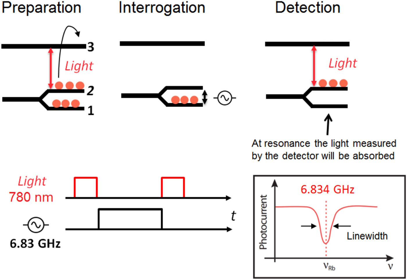
Fig. 1. Atomic resonance in the 87Rb atom applied in the pulsed regime. The atoms are represented by a three-level system. The oscillator is created by cycles of absorption and emission between levels 1 and 2 and is driven by magnetic field tuned to the frequency of the transition at approximately 6.834 GHz. The oscillation signal can be distinguished only when there is a population imbalance (population inversion) between the levels 1 and 2. Laser light tuned to the transition 2–3 is both used to create the required population inversion and to detect the resonance.
The operation of the pulsed clock consists of three stages, separated in time: preparation, interrogation, and detection. Without any external EM field applied, the Rb atoms will have electrons populating levels 1 and 2 (see Fig. 1). Because the energy difference between the levels is small (which can be related to the transition frequency as: f 1,2 = (E 2 − E 1)/h = ΔE 1,2/h, where E 1 is the energy associated to the ground state, E 2 is the energy associated to the excited state, h is the Planck's constant, and f 1,2 is in the GHz range), the energy distribution in a thermal vapor results in equally populated levels. This can be overcome in the preparation stage by applying a light pulse that is resonant to the energy difference between levels 2 and 3 (optical transition). After a given time, most of the atoms are excited and level 2 is depopulated; hence, a two-state oscillator is formed that can be used as a clock. After the laser is switched off, a resonant microwave magnetic field is applied to the atoms by the cavity in order to drive the atomic resonance (Fig. 1 – interrogation). For the atomic species considered in our case (87Rb), the frequency corresponding to the selected clock transition is f clock = f 1,2 ≈ 6.834 GHz. The atomic states 1 and 2 of the atoms can be classically seen as magnetic dipoles that according to the populated level (1 or 2) are characterized by opposite directions of the total magnetic dipole moment. Although this classical interpretation is not fully valid (in contrast to the classical view, the orientation of the atomic magnetic dipoles is quantized), it is sufficient to get qualitative understanding. Only when the microwave frequency is resonant to the energy difference ΔE 1,2, the electrons will populate the “empty” level 2 (associated with a 180° flip of the magnetic dipoles). Finally, a laser pulse of light can be applied again, and large amount of light photons will be absorbed by the electrons that now populate level 2 (Fig. 1 – detection). Therefore, by cycles of sweeping the microwave magnetic field and detecting the light absorption (the absorption line obtained from the photo-detector – Fig. 1), we can constantly lock the frequency of the input signal to the magnetic resonance transition, and hence stabilize the clock's output frequency. Because the energy levels are in reality degenerate, the exploited magnetic resonance transition needs to be well defined, and hence additional static magnetic field (C-field) is applied to the atoms – Zeeman splitting.
The above-explained EM field–atom interaction is physically realized in the physics package of the clock for which a schematic can be seen in Fig. 2. We note that the microwave cavity is the component with the largest volume, and hence it can predetermine the footprint of the final device (here we omitted the presence of a protective magnetic shield that surrounds the cavity, which is nevertheless determined by the size of the cavity).
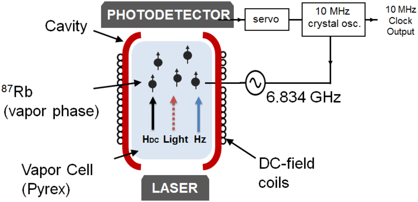
Fig. 2. The rubidium atoms in vapor phase are enclosed in a dielectric cell (Pyrex) situated inside the microwave cavity. Two apertures allow the laser light to penetrate, interact with the atoms, and get detected by the photo-detector. The C-field required for the Zeeman splitting is created by the coils surrounding the cavity oriented in the z-direction.
III. MICROWAVE CAVITIES
For a Rb atomic clock, the most important requirement on the microwave cavity is to provide all atoms with a microwave field that is well defined. Due to atomic selection rules, only the magnetic field component aligned with the direction of the C-field can drive the clock transition (at 6.834 GHz), and hence will contribute to the beneficial signal. Usually, it is most practical for both the vapor cell and the cavity to have similar shapes. One often preferred type of microwave cavity is the one of a simple hollow cylindrical shape [Reference Godone, Micalizio, Levi and Calosso8], fabricated from a metal and thus approximating the perfect electric conductor (PEC) BCs for the microwave field. In this cylindrical geometry, the vapor cell can be easily accommodated, and the coils required for the static magnetic field can be precisely machined directly to the walls. In principle, for the case of translational symmetry and PEC BCs, one can always design a cylindrical cavity that resonates at the frequency of interest f clock starting from arbitrary radius a and obtaining the corresponding cavity height d(a). Here, the only requirement is a ≥ a cutoff , where the latter is the minimum radius needed for the propagation of a guided wave at f clock for the mode of interest. Therefore, we have a possible range of cavities with different aspect ratio (AR; defined as: AR = 2a/d, where a is the radius and d is the length of the cavity) that can be used.
In this section, we will now discuss the relatively simple example of a cavity with cylindrical geometry loaded with cylindrical vapor cell (Fig. 3), and use it to introduce several design considerations and figures of merit of relevance for cavities for atomic clocks. Such cylindrical cavities are a good example often applied in double-resonance atomic clocks, and the TE011-type mode is the preferred choice since large amount of the H z magnetic field can be easily aligned to both the C-field and the laser light (as seen from Fig. 2). In the context of vapor-cell clocks, the performance of this structure is well investigated [Reference Godone, Micalizio, Levi and Calosso8] and can be assumed as a reference. From an engineering point of view, this cavity is very well known for which analytical solution is available in any good textbook [Reference Pozar9]. It is worth noting that since the dielectric walls of the vapor cell are relatively thin, the mode can be considered unperturbed for the goal of the current study [Reference Godone, Micalizio, Levi and Calosso8]. Nevertheless, a more extensive treatment is possible where the loading effect of the vapor cell can be additionally modeled [Reference Cameron, Mansour and Kudsia10].
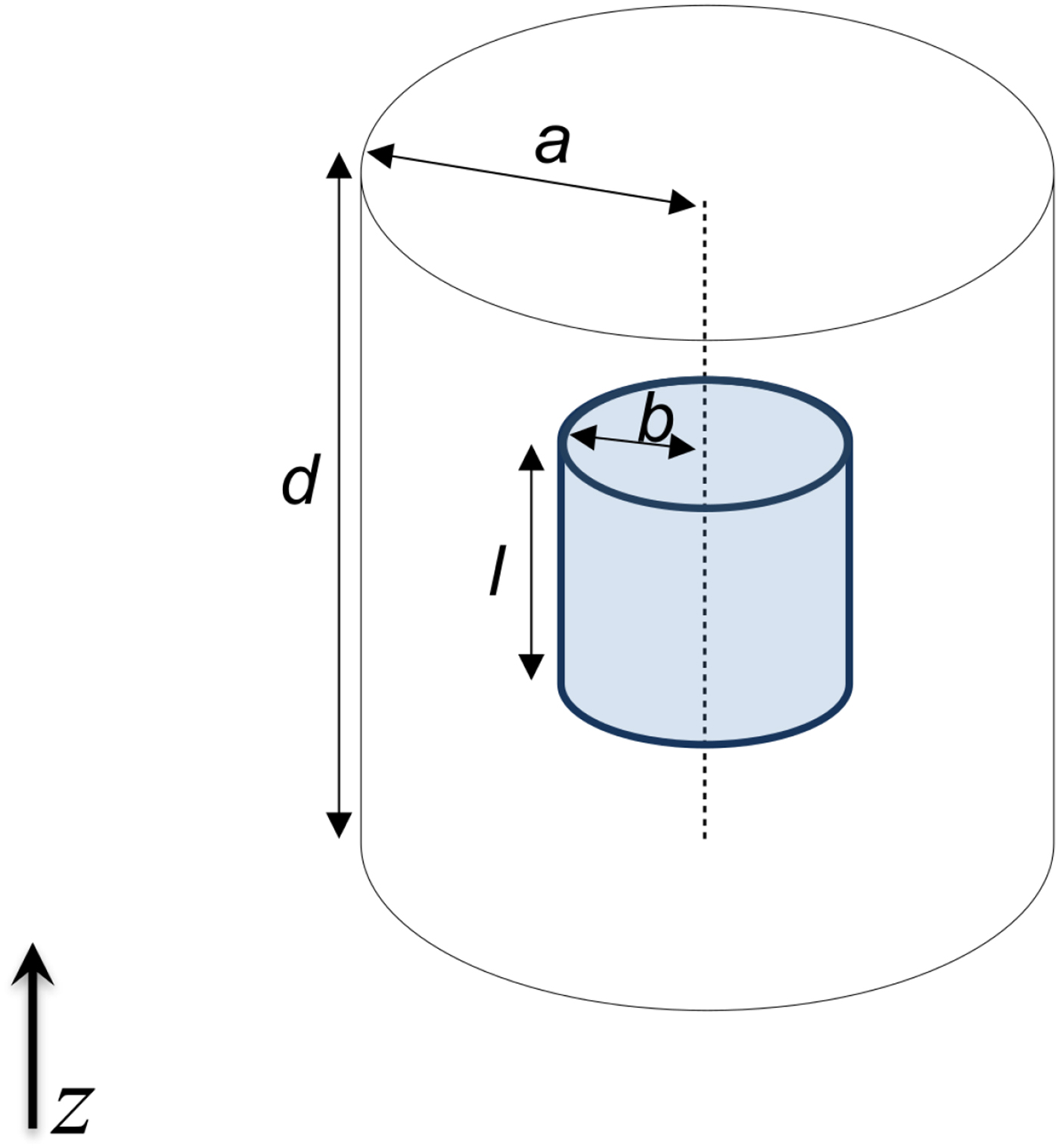
Fig. 3. Scheme of cylindrical cavity loaded with vapor cell (shown in blue). The position of the cell is chosen such that large fraction of the atoms inside the cell can interact with the B z component – TE011 mode is assumed.
A) Design guidlines and figures of merit
For the case of the Rb clock, the frequency stability can be related to the atomic Q-factor and the signal-to-noise ratio [Reference Vanier and Bernier11]:
 $$\sigma = \displaystyle{{0.2} \over {Q_a(S/N)}}\tau ^{ - (1/2)},$$
where σ is the standard Allan deviation defined for integration time τ, and Q a ≈ 107 is the Q-factor related to the atomic resonance (different from the cavity Q-factor). It can be readily seen that the design of the cavity should allow high signal-to-noise ratio and at the same time should allow for a high Q a associated to the atomic resonance. In the following, we will discuss two main properties of the microwave cavity, which both impact on the clock signal amplitude and thus on the clock stability: the uniformity (orientation) of the microwave field supported inside the cavity, and the homogeneity (in amplitude) of the same field.
1) FIELD UNIFORMITY
For the double-resonance regime in our case, the atomic response is characterized by three resonance transitions: σ −, π, and σ + that are driven by the field quantities B −, B π , and B +. The latter are referred as “driving fields” and are defined as function of the standing magnetic field provided at a given point r inside the volume of the vapor cell [Reference Affolderbach, Du, Bandi, Horsley, Treutlein and Mileti12]:
 $$\matrix{ {B_ - ({\bi r})} \hfill & { = \displaystyle{1 \over 2}(B_x({\bi r}) + jB_y({\bi r})),} \hfill \cr {B_\pi ({\bi r})} \hfill & { = B_z({\bi r}),} \hfill \cr {B_ + ({\bi r})} \hfill & { = \displaystyle{1 \over 2}(B_x({\bi r}) - jB_y({\bi r})).} \hfill \cr} $$
The direction of the static magnetic field B c (the quantization axis) is considered to coincide with the z-axis, hence B π ≡ B z . Therefore, the chosen transition used for clock operation, in our case the “π” component, is driven only by the longitudinal magnetic field H z [Transverse Electric (TE) mode is considered]. In the case of the simple cylindrical geometry, it is straight-forward to calculate the field distribution and to directly obtain the corresponding driving fields (Fig. 4).
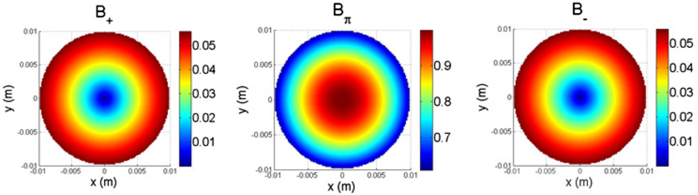
Fig. 4. Simulated 2D field profiles corresponding to the driving fields that interact with the atoms inside the vapor cell. The field amplitudes are averaged along the direction of the laser light – z and are shown normalized to the maximum found in the center for in case of the TE011 mode. Each component is color-coded separately.
One way to improve the signal-to-noise ratio is to increase the fraction of Rb atoms that interact with the proper driving field. Therefore, a good design is able to provide only the required B π component over the biggest possible volume of the vapor cell and both B − and B + are negligible. From Fig. 4, it can be qualitatively seen that while the biggest part of the magnetic field in the cavity is attributed to the clock transition, part of the field drives the unwanted σ − and σ + transitions. In Fig. 5, we show the contribution of the unwanted transitions to the total optical signal, here detected in continuous-wave double-resonance mode.

Fig. 5. Zeeman-split spectrum of the atomic microwave transition, recorded in continuous-wave double-resonance mode. The central line around zero frequency detuning corresponds to the required clock transition for which the cavity needs to be designed to maximize.
In order to be able to quantify this effect, we can introduce a figure of merit known as Filling Factor (FF), traditionally used to describe the amount of cavity–atom coupling in active masers [Reference Vanier and Audoin13]:
 $${\rm FF} = \displaystyle{{V_{Rb}{\langle \vert H_z \vert \rangle} ^2_{Rb}} \over {V_{cavity}{\langle \vert {\bi H} \vert ^2\rangle} _{cavity}}} = \displaystyle{{{\left( {\int_{V_{Rb}} \vert H_z \vert dv} \right)}^2} \over {V_{Rb}\int_{V_{cavity}} \vert {\bi H} \vert ^2dv}}.$$
Physically, it describes how much of the total microwave field energy supported by the cavity can couple to the clock transition, where the 〈 〉 Rb and 〈 〉 cavity correspond to averaging over the related volume with all volume elements considered having equal weight and static magnetic field defined along the z-axis such that |H z | ≡ |H π |. For the conditions in a maser, the atoms are in random motion over the entire volume of the cell and hence see the spatially averaged strength of the standing wave field. In equation (3), this effect is considered in the numerator, where 〈|H z |〉2 is the square of the average over the cell volume. It is known that in vapor-cell clocks, due to the buffer gas added to the cell, the atoms can be considered spatially localized for timescales relevant for the double-resonance signal [Reference Stefanucci14]. Therefore, hereafter, it is appropriate to consider figures of merit that explicitly take into account such localized-atom approximation. For completeness, the standard definition of FF can be modified for the case of localized atoms [Reference Vanier and Audoin13, Reference Major15]:
 $${\rm F}{\rm F}_s = \displaystyle{{V_{Rb}{\langle \vert H_z \vert ^2\rangle} _{Rb}} \over {V_{cavity}{\langle \vert {\bi H} \vert ^2\rangle} _{cavity}}} = \displaystyle{{\int_{V_{Rb}} \vert H_z \vert ^2}dv \over {\int_{V_{cavity}} \vert {\bf H} \vert ^2}dv}.$$
In order to obtain a measure of the field orientation across the vapor cell, more appropriate for double-resonance atomic clocks, a field orientation factor (FOF) can be defined as in [Reference Stefanucci14]:
 $${\rm FOF} = \displaystyle{{\int_{V_{Rb}} \vert H_z \vert ^2}dv \over {\int_{V_{Rb}} \vert {\bi H} \vert ^2}dv}.$$
One advantage of this figure of merit is that it can be experimentally verified – the experimental FOF can be obtained from the equation [Reference Stefanucci14]:
 $${\rm FO}{\rm F}_{exp} = \displaystyle{{\int \!S_\pi df} \over {\int \!S_\pi df + \int \!S_{\sigma _ -} df + \int \!S_{\sigma _ +} df}},$$
where $\int S_\pi df$
and
$\int S_\pi df$
and $\int S_{\sigma _{ +,} \sigma _ -} df$
can be determined from the detected optical signal and correspond to the signal transmission strength that can be obtained by integration of the curves along the frequency detuning (Fig. 5). While the FF shows how much of the cavity field is used, the FOF is related to the quality of H-field orientation inside the active volume of the cavity, and hence it is directly related to the clock signal. In Fig. 6, we relate the above-mentioned figures of merit to the case of the TE011 cavity. In our microwave design considerations, cavities with lower AR are generally more efficient because a large relative part of their energy is attributed to the H
z
component. In Fig. 6, the selected range corresponds to somewhat practically realizable geometries with ARs: 0.7 ≤ AR ≤ 2 for which the volume of the cavity is minimized, while the degradation in cavity Q-factor related to losses due to finite conductivity of the walls is the lowest. It is evident that the amount and the quality of the driving field provided to the atoms is also related to the vapor cell – in Fig. 7, we show the dependence of the figures of merit on the cell dimensions.
$\int S_{\sigma _{ +,} \sigma _ -} df$
can be determined from the detected optical signal and correspond to the signal transmission strength that can be obtained by integration of the curves along the frequency detuning (Fig. 5). While the FF shows how much of the cavity field is used, the FOF is related to the quality of H-field orientation inside the active volume of the cavity, and hence it is directly related to the clock signal. In Fig. 6, we relate the above-mentioned figures of merit to the case of the TE011 cavity. In our microwave design considerations, cavities with lower AR are generally more efficient because a large relative part of their energy is attributed to the H
z
component. In Fig. 6, the selected range corresponds to somewhat practically realizable geometries with ARs: 0.7 ≤ AR ≤ 2 for which the volume of the cavity is minimized, while the degradation in cavity Q-factor related to losses due to finite conductivity of the walls is the lowest. It is evident that the amount and the quality of the driving field provided to the atoms is also related to the vapor cell – in Fig. 7, we show the dependence of the figures of merit on the cell dimensions.

Fig. 6. Figures of merit for the TE011 cylindrical cavity as function of the cavity dimensions (radius – a, height – d). Two cylindrical vapor cells are considered: “small”, b = 10 mm, l = 20 mm; large, b = 11 mm, l = 23 mm (Fig. 3).
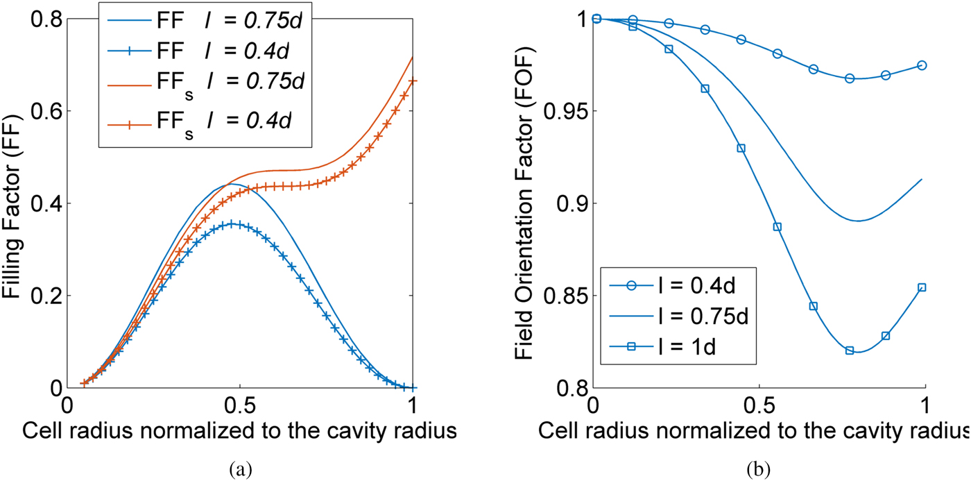
Fig. 7. Figures of merit for the TE011 cylindrical cavity as function of the cell dimensions. The results are shown for a cavity with fixed dimensions (AR = 1), l is the height of the vapor cell, normalized to the height of the cavity d. For the mode of interest, the distribution of the favorable H z field is such that a phase change occurs at radius ≈ 0.62a, independent on the chosen AR. Therefore, the size of the vapor cell to be considered is according to 0 ≤ b ≤ 0.62a.
It can be seen that the design close to optimal corresponds to cavities with AR in the range 1–1.5. Because the unwanted driving fields are mostly present away from the center, in the vicinity of the top and bottom caps, the FOF can be very high for vapor cells with low volume when cavities with lower AR are assumed. We consider a cavity with AR of 1 and a cell with AR of 0.5 and dimensions radius =10 mm and length =20 mm as a reference structure.
2) HOMOGENEITY OF THE FIELD AMPLITUDE
The homogeneity of the microwave field amplitude H z across the vapor cell is of high importance for the signal-to-noise ratio and thus for the achievable clock stability. In fact, any variations in H z result in a part of the localized atoms experiencing incomplete transitions during the interrogation phase in pulsed clock operation mode (Fig. 1), resulting in a reduction of clock signal amplitude. The spatial distribution of the field is subject to BCs, and hence it is impossible for the ensemble of atoms to interact with equal field amplitude. Furthermore, position-dependent microwave power shift of the clock transition can lead to inhomogeneous broadening of the clock signal, which may reduce Q a and degrade the clock stability (see equation (1)). The field homogeneity is therefore an important characteristic that needs to be specifically targeted in the cavity design.
A direct way to estimate the homogeneity associated to a given structure is to numerically obtain a two-dimensional (2D) field map and to plot the isoclines (contour plot). This approach is intuitive but has limited application since we often want to compare very different geometries. Instead, a field histogram approach known also in the magnetic resonance community [Reference Li, Yang and Smith16] is suitable to apply in order to assess the field homogeneity. In this case, the H z field is uniformly sampled over the active volume of the cavity with resolution allowing accurate representation of the spatial variation. The obtained distribution of field amplitudes is normalized to the maximum found in the center of the cavity. The relative number of sampled points with field amplitudes in a chosen variation range corresponds to the amount of volume inside the cell that sees field with the corresponding variation. Therefore, since the atoms are considered static and uniformly distributed, this volume corresponds to the relative amount of atoms.
For a cavity based on a translational symmetry, it is evident that the field distribution can be separated into transverse – along the diameter, and longitudinal – along the height. The intrinsic field variation associated to the transverse direction is predetermined by the shape of the cross-sectional BC, and for the case of the TE011, cylindrical cavity can be seen represented by the dashed curve in Fig. 8(a). As can be expected, the sinusoidal field dependence along the z-axis degrades the homogeneity – the solid curve in Fig. 8(a). It is evident that the homogeneity of the field available to the vapor is increased if the volume of the vapor cell is reduced.

Fig. 8. Variation plot of the H z field amplitude calculated based on the field histogram approach. The amount of active volume that can be attributed to the normalized variation of the field amplitude: (1 − |H z |/(|H z |) max ) is shown. For example, 0.4 on the x-axis of plot (a) corresponds to the range (|H z |) max ≤ x <0.4(|H z |) max , and hence from the plot, it can be interpreted that about 70% of the atoms in the volume will interact with |H z | field that varies by not more than 40% from the maximum. The results are calculated for a cylindrical vapor cell, situated in the center of the cavity and with standard dimensions: radius – 10 mm, length – 20 mm.
In this section, we showed from an engineering point of view which physical mechanisms relate the cavity to the stability of the clock. Corresponding figures of merit were introduced and related to the basic cylindrical geometry in order to gain general understanding about the optimal design of the cavity as well as the size of the cell. The requirement for high signal-to-noise ratio and hence large active volume V Rb means that the larger the vapor cell, the more signal is available to the clock transition (higher FF); however, the unwanted transitions are coupled more (lower FOF) and the homogeneity is also degraded. Therefore, a trade-off exists between the size of the vapor cell and the amount of useful field provided by the chosen cavity geometry. Finally, we note that the results obtained correspond to the simplified case where the cell is assumed with zero thickness, field leakage from the apertures is not considered, PEC BCs and single mode are assumed, and the optical density attributed to the Rb vapor is not taken into account.
IV. LOOP-GAP GEOMETRY
In Section III, it was explained that the cylindrical cavity allows satisfactory performance and is the common choice for vapor-cell clocks. However, the volume of the cell is typically <5% of the cavity volume. This inherent limitation of the simple cylindrical geometry can be overcome if the cavity is additionally loaded. A very efficient way to reduce the dimensions is to consider a loop-gap structure [Reference Froncisz and Hyde17], also known in the literature as slotted-tube [Reference Sphicopoulos and Gardiol18] or magnetron-type resonator [Reference Stefanucci14, Reference Chen, Li, Liu and Gao19]. It consists of a cylindrical volume filled with metal electrodes, which can be seen as a combination of capacitance and inductance (Fig. 9). Such a design is very flexible since a number of parameters can be tuned in order to obtain the resonance condition. Physically, the volume can be reduced for the mode of interest mainly because the balance of electric and magnetic energy associated to resonance is achieved through the electrode structure and is less restricted by the overall volume. Typically, such geometries have a reduction of the volume between three and four times compared with the standard cylindrical geometry, while the useful volume of the cavity is about 25%. In Fig. 8(b), we show the calculated field variation attributed to the general design shown in Fig. 9. It can be seen that the 2D distribution (in the transverse plane) associated to the cross-section is slightly better (curve higher) than the standard cavity, i.e. a desired small (e.g. <40%) variation of field amplitude can be achieved over a bigger fraction of the cavity volume. The presence of the top and bottom boundaries degrade the homogeneity as in the case of the simple cylindrical geometry. Still, the field homogeneity for the loop-gap cavity (Fig. 8(b)) is at least comparable to the one obtained for the cylindrical cavity (Fig. 8(a)), but with a considerably smaller overall cavity volume. We note that these plots are numerically obtained and correspond to the somewhat idealized case of a geometry without apertures and further complications and assuming the transverse variation is completely determined by the transverse BC. Nevertheless, they are convenient, since the limitations in terms of field homogeneity can be related to the chosen geometry.
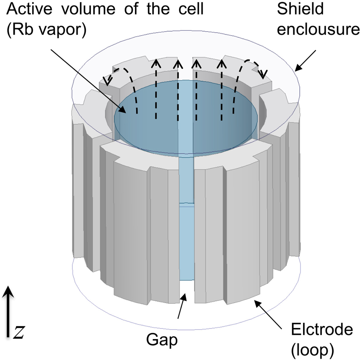
Fig. 9. Scheme of the basic structure of atomic clock cavity. The loop-gap structure is based on six electrodes. Two empty cylindrical extensions are situated on both sides of the loop-gap region. The magnetic field lines are represented by the dashed arrows. The components required for the clock operation are omitted (e.g. vapor cell, apertures required for the pumping light, optical lenses, feeding, tunning mechanism).
A loop-gap cavity was previously designed by our group [Reference Stefanucci14] for the case of high-performance double-resonance clock based on continuous type of operation (Fig. 10).

Fig. 10. Scheme of an atomic clock cavity based on a loop-gap structure [Reference Stefanucci14]. Realizations that additionally include optical lens are also possible. A variety of dielectric materials can be used for the vapor cell. A high level of customization is required due to the different structures of the condensation stems that can be used in practice.
A combination of six loops and gaps was optimized to meet the magnetic resonance condition for a low overall volume. The cavity was engineered in order to accommodate a significantly enlarged vapor cell (up to 25 mm in diameter), which is possible because of the high FOF ≈85% as experimentally confirmed in [Reference Stefanucci14]. The short-term stability of a clock based on this cavity was reported to be 1.4 × 10⁻¹³ τ −1/2 in continuous interrogation mode [Reference Bandi, Affolderbach, Stefanucci, Merli, Skrivervik and Mileti20].
In the discussion above, it was shown that it is possible to meet the stringent field requirements for a reduced volume of the cavity when an appropriate loop-gap structure is considered. Furthermore, the reduced external diameter of the loop-gap cross-section will not degrade the homogeneity of the magnetic field interacting with the atoms in the vapor cell. On the other hand, it is seen that the variation of the field along the z-direction contributes to a significant degradation of the field homogeneity, which is a characteristic of all cylindrical geometries. It is possible to address the latter by engineering BCs that can, in principle, eliminate the field variation along the height of the cavity (active volume). Therefore, a realistic realization of such a structure will be characterized by a field distribution with a variation curve corresponding to the shaded region in Fig. 8.
V. MODIFIED BOUNDARY CONDITIONS
In principle, a spatially constant field (λ g → ∞) can be obtained along the height of a generalized cylindrical cavity if the mode of interest can exist with a longitudinal mode number zero. Such a cavity resonates at the cutoff frequency related to the chosen cross-section since there is no dependence on z. For the canonical (circular) geometry, this is fulfilled, e.g. for the TM010 mode. In this case, the tangential magnetic field is unaffected by the top and bottom PEC plates, the longitudinal electric field E z is constant along z, while the transverse components E ϕ and E ρ are zero. Such TM010 cavities are often utilized in the design of band-pass filters [Reference Kobayashi and Yoshida21].
In our application, we are interested in exploiting the dual TE010 case for which the H z component is constant along z. It is easy to see that this requirement cannot be fulfilled by the PEC plates since the H z component is normal to the boundary, and therefore goes to zero at each of the two end planes. However, the homogeneous TE010 mode can exist if the complementary perfect magnetic conductor (PMC) BC is applied, where in this case, it is the transverse magnetic field that is zero. The latter is an additional advantage for our application since the unwanted atomic σ − and σ + transitions are not driven in such a cavity (see equations (2) and (5)).
The engineering of artificial BCs, also known as artificial magnetic conductor (AMC), high-impedance surface, or magnetic mirrors (in optics), has been an active topic of research for various applications mostly related to miniaturization in antennas [Reference Feresidis, Goussetis, Wang and Vardaxoglou22] and microwave devices [Reference Dancila, Rottenberg, Focant, Tilmans, De Raedt and Huynen23]; improvement of the field homogeneity in the case of electron paramagnetic resonance [Reference Mett, Froncisz and Hyde24–Reference Mett, Sidabras and Hyde27], as well as for the use in quantum experiments [Reference Gurman28] and optical applications [Reference Pisano, Ade and Tucker29]. We briefly discuss the general idea of a cavity with AMC BCs by first assuming the simple cylindrical geometry discussed in Section III.
A) Simple cylindrical geometry with AMC boundaries
One way to obtain AMC boundaries is to include symmetric dielectric segments at the top and at the bottom of the cavity interior as shown in Fig. 11 (PEC condition is considered for the outer surface of the cavity). The height of the dielectric segments depends on the chosen material, and for the cylindrical cavity, it is possible to be obtained analytically [Reference Mett, Froncisz and Hyde24]:
 $$e_a = \left( {\displaystyle{{\mu _0{\epsilon} _0} \over {{\epsilon} _r - 1}}} \right)^{1/2}\displaystyle{1 \over {4f_{cut}}},$$
where f cut is the cutoff frequency and ε r is the relative dielectric constant attributed to the dielectric material. Physically, e a corresponds to the 1/4 of the guided wavelength considered in the dielectric. While a PEC plane reflects the reversed in phase electric field and is hence characterized by reflection coefficient –1, in the case of PMC the latter is unity. The dielectric segment can be therefore seen as a resonance structure for which multiple reflections add up such that reflection coefficient unity is seen by the standing wave in the central region of the cavity. In principle, if the condition given in equation (7) is fulfilled, the TE010 mode in such a cavity is independent on the distance d (shown in Fig. 11) and hence for the resonance frequency we have: f res = f cut . In Fig. 12, we show the amplitude of the numerally obtained B π driving field as function of the dielectric filling.
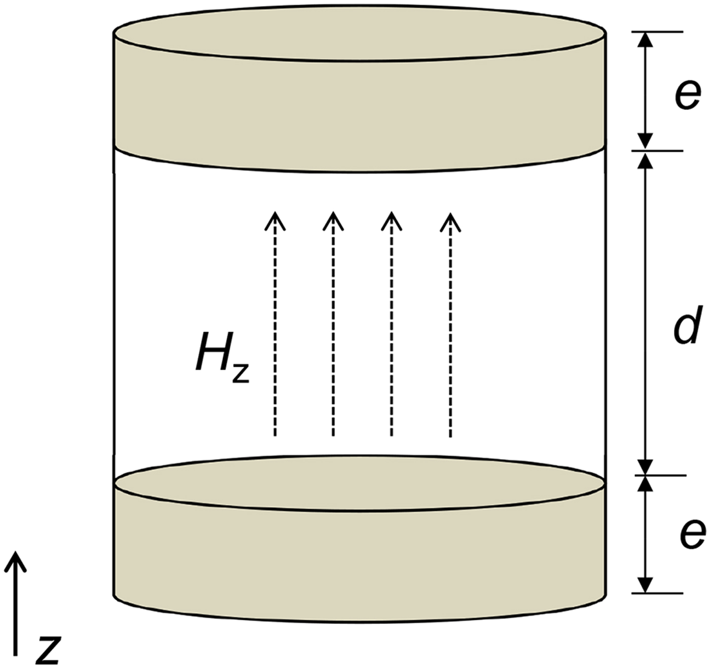
Fig. 11. Scheme of a fully enclosed cavity loaded with dielectric segements with height e. The AMC boundary conditions, for which the mode in the central region (considered empty) is TE010, have length e = e a given in equation (7).
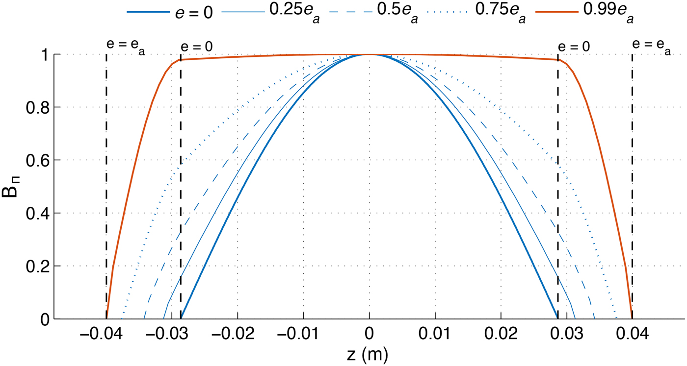
Fig. 12. Field distribution of the B π component along the central axis of a cavity loaded with dielectric segments with different height e. The vertical dashed lines define the dimensions of the standard empty cavity (e = 0) as well as the TE010 case: e = e a . All field components are normalized to the maximum for the B π amplitude found in the center. The dielectric material considered is with ε r = 2, for which the length e a that fulfills the TE010 condition is obtained from equation (7) and is e a ≈ 11.9 mm. The field in the central region is nearly constant (shown in red) for e = 0.99e a .
It can be readily seen that such a modification of the BCs is beneficial in the context of our application: the field homogeneity can be significantly improved, the FOF is close to unity, the volume of the cavity can be reduced without affecting the resonance frequency, a cavity with lower AR can be used. In order to provide access for the laser required for optical pumping, a dielectric material can be chosen that is transparent for the light (e.g. Pyrex). Furthermore, apertures are needed at the top and bottom of the metal enclosure. In the above analysis, they are neglected, assuming that for the mode of interest, they can be made close to non-radiating by adding additional under-cutoff pipes. Although the loaded Q-factor is reduced with respect to the standard geometry (extensive analysis can be found in [Reference Mett, Froncisz and Hyde24]), we note that in our application, the cavity Q-factor is not a critical parameter. Values of Q loaded <200 are in principle enough to meet the requirements of clocks based on double resonance [Reference Stefanucci14].
In order to be able to properly apply such AMC BCs to the case of more complicated geometries like the loop gap, we have chosen to use a combination of transmission line (TL) model and full-wave simulations based on finite element method (FEM).
B) Transmission line model
It is known that when the mode inside the cavity is well defined, the resonance condition can be obtained by a TL model (the same approach is often used to find transverse resonances and is also known as transverse resonance method). In this case, each cavity segment can be described via its corresponding length, characteristic impedance, and propagation constant attributed to the propagating mode (Fig. 13(a)). It can be shown that at resonance, for the left-oriented $\overleftarrow Z _{in}$
and right-oriented
$\overleftarrow Z _{in}$
and right-oriented $\overrightarrow Z _{in}$
input impedance, we have the equality
$\overrightarrow Z _{in}$
input impedance, we have the equality $\overleftarrow Z _{in} = - \overrightarrow Z _{in}$
, which can be defined for a chosen coordinate z along the TL. It is then straight-forward to express the above-described condition in terms of TL parameters:
$\overleftarrow Z _{in} = - \overrightarrow Z _{in}$
, which can be defined for a chosen coordinate z along the TL. It is then straight-forward to express the above-described condition in terms of TL parameters:
 $$\tan ({\beta} ^{\prime}d) = \displaystyle{{{{Z}^{\prime}}_c(Z_{c,1}\tan (\beta _1e_1) + Z_{c,2}\tan (\beta _2e_2))} \over {Z_{c,1}Z_{c,2}\tan (\beta _1e_1)\tan (\beta _2e_2) + {({{Z}^{\prime}}_c)}^2}},$$
where the characteristic impedances and the propagation constants in the two dielectric segments and the central region are given by: Z
c,1, Z
c,1, ${Z}^{\prime}_c$
and β
1, β
2, β′ correspondingly (Fig. 13(a)). In the above equation, for the length of the middle region, we have used: d
1 = 0, d
2 = d, which is possible since we are free to choose the z-coordinate. If two identical dielectric segments are considered we have: Z
c,1 = Z
c,2 = Z
c
; β
1 = β
2 = β; e
1 = e
2 = e, and hence equation (8) reduces to:
${Z}^{\prime}_c$
and β
1, β
2, β′ correspondingly (Fig. 13(a)). In the above equation, for the length of the middle region, we have used: d
1 = 0, d
2 = d, which is possible since we are free to choose the z-coordinate. If two identical dielectric segments are considered we have: Z
c,1 = Z
c,2 = Z
c
; β
1 = β
2 = β; e
1 = e
2 = e, and hence equation (8) reduces to:
 $$\tan ({\beta} ^{\prime}d) = \displaystyle{{2{{Z}^{\prime}}_cZ_c\tan (\beta e)} \over {Z_c^2 \mathop {\tan} \nolimits^2 (\beta e) + {({{Z}^{\prime}}_c)}^2}}.$$
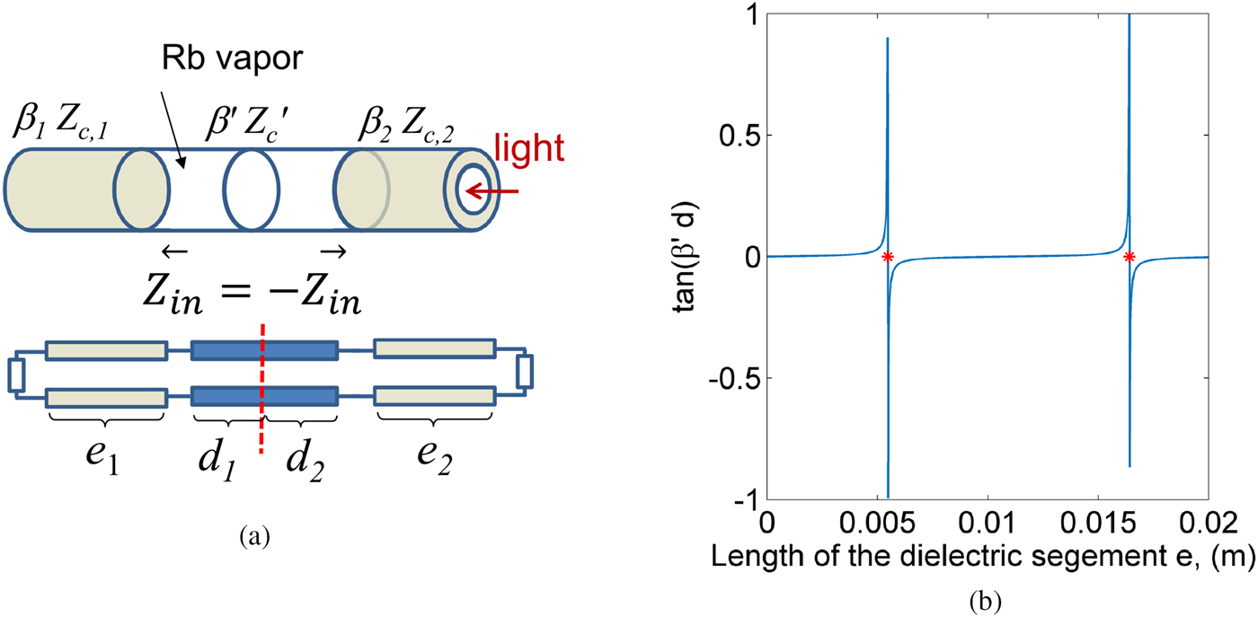
Fig. 13. Transmission line model and numerically obtained solution for the transcendental equation (9). The roots are indicated with red markers and correspond to the first two solutions found for the length e for which the dielectric segments appear as AMC boundary condition. The calculated result corresponds to the previously discussed cavity geometry – Fig. 12 and confirms the result obtained via equation (7).
For the homogeneous mode, we are interested in the limit case: f res = f cut ⇒ λ guided → ∞, and for the propagation constant in the middle region, we have β′ → 0. It is therefore possible to use equation (9) in order to find the unknown distance e, for which the homogeneous mode is defined (Fig. 13(b)).
The main assumptions that need to be taken into account are: single-mode propagation is considered, higher order modes are neglected, and hence discontinuities need to be treated with caution. Losses are not considered, and hence the load impedance in Fig. 13(a) is imaginary. The latter requirement is natural since the TL model is related to the eigensolution, and hence sources or losses are not defined. The apertures can be taken into account by assuming long enough under-cutoff extensions for which the load impedance is purely imaginary. In the case of the loop-gap structure, the propagation constant can be obtained via equivalent models based on lumped elements [Reference Mett, Sidabras and Hyde27, Reference Hyde, Froncisz and Oles30] or alternatively by a FEM simulations (ANSYS HFSS is preferred for the results shown in this study).
C) Implementation of tuning in the case of AMC
Since the homogeneous mode is in principle independent on the height, a standard solution based on the electrical length is not optimal. In this case, frequency tuning can be obtained by directly changing the cutoff in the central region or by perturbing the AMC boundaries. In order to be physically understood, we apply perturbation theory that was initially developed to study the sensitivity in the canonical case [Reference Mett, Froncisz and Hyde24]. Assume that the height of the dielectric segments e is chosen to vary slightly from the optimal: e = e a ± e′, where e a is the condition to obtain AMC given by equation (7), and e′ is a small dimension variation. In this case, a deviation from the expected homogeneous field is observed (Fig. 14).

Fig. 14. The plots show the effect of the dielectric length on the H z distribution in the homogeneous region of the cavity. The result is calculated for the central axis of a TE010 cavity with radius of 26.7 mm and length of 36.6 mm. Dielectric with ε r = 5 is considered. The field profiles are normalized with respect to the center of the cavity, and the constant field distribution corresponding to the ideal AMC case is shown in red.
In the first case (Fig. 14(a)), the field shows slight sinusoidal variation similar to the case of PEC boundaries, and therefore the resonance frequency is increased. In the second case (Fig. 14(b)), the field in the central region is slightly evanescent – the peak of the field is pulled toward the dielectric for which propagation starts lower in frequency. Therefore, in this case, the TE010 mode is characterized by a resonance frequency slightly lower than the cutoff frequency. Since the AMC can be modeled as a parallel LC circuit, calculated for the volume of the dielectric segment, we have W e = W h , where W e and W h stand for the electric and magnetic energy. Equivalently for the dielectric volume of the perturbed AMC can be calculated that in the first case we have Wh > We while in the second case we have We < Wh . It is now evident that the process of tuning can be associated with energy imbalance in the AMC.
VI. LOOP-GAP CAVITY WITH AMC BOUNDARIES
As explained in Section II, besides the loop-gap electrodes, various other components are needed for the clock operation. This, combined with the compact volume of the cavity results in a somewhat highly packed structure (Fig. 10) for which realization of AMCs is a very challenging task. Typically, the process used to produce the dielectric cell is prone to considerable tolerances. This is a significant problem because the TE010-type mode is operating at the limit case and is hence characterized by high geometrical sensitivity. Large light apertures and additional openings are required for the condensation stem of the cell (one or two depending on the cell structure), which make it difficult to meet the ideal performance from Fig. 12. Furthermore, the position of the feeding mechanism (usually a small loop at the bottom – Fig. 10) is often limited by the presence of the external magnetic shielding. The latter is a major complication for the suppression of unwanted modes. Finally, the design should be universal enough to allow cells with structural differences.
A) Planar AMC
Alongside the AMC implementation based on dielectric filling, we have previously considered an alternative planar solution [Reference Ivanov, Skrivervik, Affolderbach and Mileti31] that can be used to improve the flexibility. Here we discuss in further detail a general design criterion required for its realization.
A common trait among the implementations of AMC is the utilization of some resonant behavior. In this sense, it is advantageous that the generic structure of the loop-gap cavity is characterized by a longitudinal impedance discontinuity (see Fig. 9). For the mode of interest, the standing wave exists in the central region but is under cutoff in the cylindrical extensions situated on both sides. However, since part of the field (mostly magnetic) leaks in the extensions, it is natural to assume that they can be engineered, so that a unity reflection coefficient can be locally found. In our case, this cannot be obtained by changing the external radius or shape of the cross-section (due to the complicated structure of the physics package: dc coils, heating required for the vapor, magnetic shielding). It is instead possible to utilize a loop-gap structure similar to the one already used in the central region of the cavity. Furthermore, for practical reasons, it is favorable to use a planar design where the metal loops (electrodes) can be directly etched on a dielectric substrate that in this case is only used for support (Fig. 16). In principle, the loop-gap structure can be described via its circuit equivalents [Reference Froncisz and Hyde17]:
 $$C = \displaystyle{{{\epsilon} wz} \over {tn}},\quad L = \displaystyle{{\mu _0\pi r^2} \over z},$$
where C and L are the approximated capacitance and inductance, r is the internal radius of the loop-gap region, n is the number of gaps, t is the length of the gap, w is the thickness of the loop elements, and z is the height (Fig. 16(b)). Since C and L scale opposite with z, the intrinsic frequency associated to the loop gap is described by only the transverse dimensions and is given by:
 $$\eqalign{& f_{int} = \displaystyle{1 \over {2\pi}} \sqrt {\displaystyle{{nt} \over {\pi r^2{\epsilon} \mu w}}} \sqrt {1 + \displaystyle{{r^2} \over {R^2 - {(r + w)}^2}}} \cr & \;\;\;\;\;\;\sqrt {\displaystyle{1 \over {1 + 2.5t/w}}},} $$
where the first term is the resonance frequency of the LC circuit and the two other terms improve the approximation by accounting for the effect of the metal shield and the fringing fields accordingly [Reference Froncisz and Hyde17]. Although approximate, these expressions are found to describe relatively well the loop gap for the mode of interest (Fig. 15).
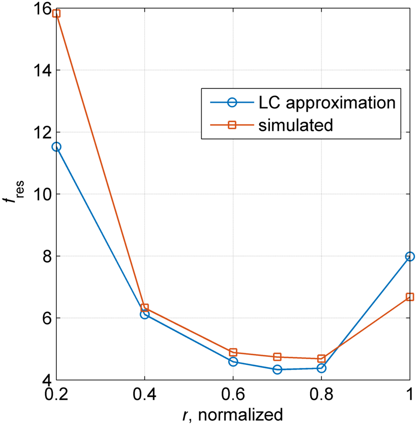
Fig. 15. Intrinsic resonance frequency associated to the loop-gap structure as function of the internal radius r. All dimensions are as the reported in Table 1, the normalization is according r = 16.8 mm. The outcome of equation (11) is compared to a result from full-wave eigen simulation performed via ANSYS HFSS. By applying PMC boundaries at both planes of the loop-gap cross-section, the numerically found frequency has the same physical meaning as the modeled in equation (11).
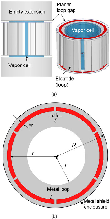
Fig. 16. Loop-gap cavity with AMC boundaries based on planar structures.
Table 1. Dimensions of the planar loop gap.

We can use the above-described way to design the planar loop gap to resonate close to the requirement: f int ≈ f clock . It is appropriate to consider the interval of normalized radius r >0.6 (Fig. 15) because of the requirement for the light apertures. Placing it in the vicinity of the electrodes (as seen in Fig. 16(a)) couples it to the central loop-gap region since both structures support the mode of interest. While in principle, the coupling problem is complicated to model, it is clear that the magnetic field leaking out of the central region contributes the most. Therefore, it is mainly the distance between the planar structure and the main loop-gap region that controls the amount of coupling. In our case, due to structural reasons, it is preferred to fix the planar loop gap close to the top and bottom walls of the vapor cell. From a TL point of view, the AMC boundary corresponds to an impedance Z → ∞, and hence the extensions (loaded with the planar loop gap) can be modeled as a parallel LC circuit. Since we consider the planar AMC to apply at both ends of the central region, the magnetic/electric energy integrated over the whole volume of the loaded extensions is W e = W h . However, because of the evanescent magnetic field, we have W e < W h and hence the cavity resonates above the cutoff of the central region. This can be counteracted by decreasing the intrinsic frequency of the planar loop gap since the parallel LC is capacitive for f > f int . From Fig. 15, it is clear that in this case we need to reduce the internal radius r of the planar loop gap. The balance between W e , W h is easily obtained from simulations and can be used as a design rule (Fig. 17(a)). From Fig. 17(a), it is clear that the AMC condition is obtained for r ≈ 0.72. For lower r, the field is slightly evanescent toward the extensions, and hence the cavity resonates lower than the cutoff. It is interesting to see that for the smallest radius considered, the magnetic energy starts increasing again as well as the resonance frequency of the cavity. This is because, as seen in Fig. 15, in this case, the intrinsic frequency of the planar loop gap starts increasing again.
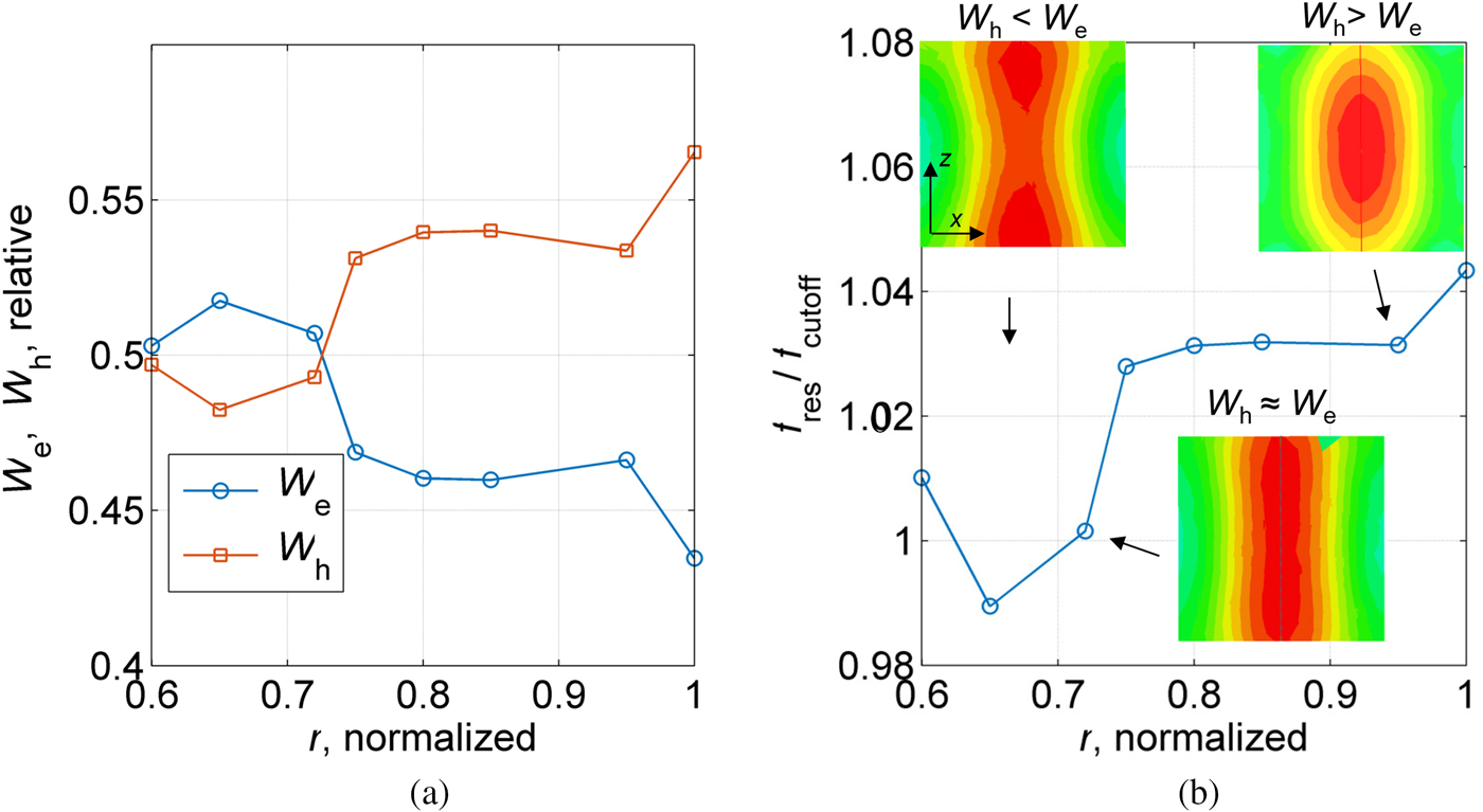
Fig. 17. The plots show what is the effect of scaling the internal radius r of the planar loop gap. For normalized radius of ≈ 0.72, the mode in the central region is TE010 and the cavity resonates at the cutoff (of the central region). All dimensions are as reported in Table 1. The height of the extensions is 14 mm, and the distance between the planar loop gap and the central region is 1 mm.
In terms of fabrication, the above-described solution is suitable since for the frequency of interest, the planar technology has generally well-controlled tolerances and negligible losses. Furthermore, it is characterized by a small footprint, and is hence less stringent to accommodate inside the cavity. A variety of such structures can be easily developed allowing to retrofit the cavity without complicated machining. On the negative side is the fact that generally the planar AMC works well when the top extensions are long enough. In Fig. 18, we report the obtained field homogeneity for two different extension lengths. It is seen that when the extensions are kept long (as reported for the case shown in Fig. 17), the field along the central axis is close to constant, while the field considered at half the cell radius is within 5% variation. When extensions with half the length are considered, the distribution for the off-centered profile is degraded significantly ( $ \approx 20\% $
variation). It is possible however to try mitigate this effect by employing a second planar structure situated above the planar loop gap and further tune the AMC condition. For a highly compacted design, a solution based on dielectric filling is found to perform better. In this case, even if short extensions are considered, we have
$ \approx 20\% $
variation). It is possible however to try mitigate this effect by employing a second planar structure situated above the planar loop gap and further tune the AMC condition. For a highly compacted design, a solution based on dielectric filling is found to perform better. In this case, even if short extensions are considered, we have $ \approx 5\% $
variation for the central and
$ \approx 5\% $
variation for the central and $ \approx 10\% $
for the off-centered profile as can be seen from Fig. 18.
$ \approx 10\% $
for the off-centered profile as can be seen from Fig. 18.

Fig. 18. Longitudinal field distribution of the B π component for a cavity based on different AMC conditions. The filed profiles correspond to the central axis as well as at half the radius of the vapor cell. The dimensions of the vapor cell are indicated by vertical lines. The height of the extensions is: 14 mm (long), 7 mm (short), 5.8 mm (dielectric AMC). The field is normalized to the maximum amplitude found separately, where in the case of dielectric AMC does not go to zero since the light apertures are very close.
Finally, it is worth noting that the cutoff frequency of the central region (the main loop gap) needs to be the targeted frequency f res . In principle, both the frequency requirement and the AMC condition need to be fulfilled at the same time – a very stringent limitation. Instead it is preferable to use a variable tuning mechanism. In this way, it is possible to obtain f res (somewhat the highest priority in the design) on the expense of slightly degraded field homogeneity.
B) Tuning mechanism
The most difficult design aspect is to insure that the resonance condition for the homogeneous mode can be met at the appropriate clock frequency. For example, due to a tolerance problem, it is possible for the homogeneous mode to be fulfilled at a significantly different resonance frequency with respect to the target one. Since we can only measure the frequency response, the cavity needs to provide a well-controlled, close to homogeneous field in a reasonable frequency range. In order to cope with this issue, we propose a mechanism that can directly tune the cutoff condition corresponding to the central region of the cavity. The idea is to include an azimuthally symmetric structure (referred as “tuning electrodes” in Fig. 19) that can be rotated with respect to the main loop-gap structure of the cavity. Therefore, by rotating the tuning electrodes, the return flux (the magnetic field in the volume between the main loop-gap electrodes and the outer cylindrical cavity shield) of the cavity can be perturbed in a symmetrical way. Because the active volume relevant for clock operation is located within the electrodes around the cavity's central axis (see Fig. 9) and due to the electrodes’ sixfold rotational symmetry, the homogeneity of the relevant field in the active volume is stable with respect to this frequency tuning method. It can be shown that in this way we are not too sensitive to a possible mismatch between the characteristics of the two AMC conditions. Furthermore, we note that since the radius of the central loop gap is relatively large, a localized transverse perturbation (e.g. a small tunning pin) cannot be utilized without a significant degradation of the required mode.

Fig. 19. Scheme of a realistic atomic clock cavity based on a loop-gap geometry and tuning electrodes. The upper part of the cylinder can be rotated (indicated by the two arrows) with respect to the fixed bottom. The main loop-gap structure of the cavity is fixed to the bottom, while the tuning electrodes (colored in blue) are attached to the inner walls of the upper cylinder and hence can be rotated. The cavity is considered for the realistic case – the cell is included with the apertures as well as appropriate feeding (not shown for reasons of clarity).
Important characteristic of the tuning mechanism is its resolution. The advantage in our case is that the thickness and the size of the tuning electrodes can be used to address the range and the resolution of the tuning. Simulation results from a preliminary study can be seen in Fig. 20. It is seen that for a range of 7 deg, the dependence is monotonous and hence can be used for frequency tuning. The tuning range in this case is close to 90 MHz, with about 13 MHz/deg, or for the dimensions used about 42 MHz/mm. It can be seen that if the size of the monotonous region is increased, the range can be further extended.

Fig. 20. Change of the resonance frequency corresponding to different rotation angles of the tuning electrodes (shown in blue) with respect to the loop gap (shown in red).
VII. FINAL DISCUSSION
In this work, we studied the possibility to use AMC-type BCs in order to significantly improve the magnetic uniformity in the microwave cavity, and hence the performance of a novel type atomic clocks based on POP. To the best of our knowledge, this is the first attempt to relate the concept of AMC to atomic clock applications.
We discussed how to relate the operation of such clock to the characteristics of the cavity. Using appropriate figures of merit, it was determined what is the optimal design in terms of clock requirements. Furthermore, we showed that a cavity based on a loop-gap structure fulfills these requirements while at the same time being significantly more compact. The general concept of AMC was introduced in the canonical case as well as a simple model that can be used to model the loop-gap case. The study covered a planar AMC solution for which we showed design criteria as well as evaluation of the performance. Finally, we consider a novel robust way of tuning that takes further advantage of the specific symmetry of the structure.
Due to its compactness and high performance, the loop-gap structure is a preferred choice for applications in vapor-cell clocks. We showed that by controlling the BCs, it is possible to further improve the performance and meet the stringent requirements for next-generation applications.
ACKNOWLEDGEMENTS
The authors acknowledge financial support from the Swiss National Science Foundation, grant number 162346.
 Anton Ivanov received his Master's degree in Engineering Physics from Sofia University, Sofia, Bulgaria in 2011, where he worked on the design and modeling of a miniature plasma source. In 2012, he joined Laboratoire d’électromagnétisme et Acoustique (LEMA) at École Polytechnique Fédérale de Lausanne (EPFL), Lausanne, Switzerland. He is currently completing his Ph.D. degree related to cavities for high-performance atomic clocks based on double resonance.
 Christoph Affolderbach received the Diploma and Ph.D. degrees in Physics from Bonn University, Bonn, Germany, in 1999 and 2002, respectively. He was a Research Scientist with the Observatoire Cantonal de Neuchâtel, Neuchâtel, Switzerland, from 2001 to 2006. In 2007, he joined the Laboratoire Temps-Fréquence, University of Neuchâtel, Neuchâtel, Switzerland, as a Scientific Collaborator. His current research interests include the development of stabilized diode laser systems, atomic spectroscopy, and vapor-cell atomic frequency standards, in particular, laser-pumped high-performance atomic clocks and miniaturized frequency standards.
 Gaetano Mileti received the Engineering degree in Physics from the École Polytechnique Fédérale de Lausanne (EPFL), Lausanne, Switzerland, in 1990, and the Ph.D. degree in Physics from the University of Neuchâtel, Neuchâtel, Switzerland, in 1995. He was a Research Scientist with the Observatoire Cantonal de Neuchâtel, University of Neuchâtel, from 1991 to 1995 and 1997 to 2006. From 1995 to 1997, he was with NIST, Boulder, Colorado, USA. In 2007, he co-founded the Laboratoire Temps-Fréquence, University of Neuchâtel, Neuchâtel, where he is currently the Deputy Director and an Associate Professor. His current research interests include atomic spectroscopy, stabilized lasers, and frequency standards.
 Anja K. Skrivervik received the Electrical Engineering degree and the Ph.D. degree from the École Polytechnique Fédérale de Lausanne (EPFL), Lausanne, Switzerland, in 1986 and 1992, respectively. After a period at the University of Rennes, Rennes, France, and in industry, she returned to EPFL as an Assistant Professor in 1996, where she is currently a Professeur Titulaire. Her teaching activities include courses on microwaves and on antennas. Her research activities include electrically small antennas, multifrequency and ultra-wideband antennas, and numerical techniques for electromagnetic and microwave and millimeter-wave microelectromechanical systems (MEMS). She is the author or coauthor of more than 100 scientific publications. She is very active in European collaboration and European projects. Dr. Skrivervik is currently the Chairperson of the Swiss International Scientific Radio Union, the Swiss representative for European Cooperation in Science and Technology action 297, and a member of the Board of the Center for High Speed Wireless Communications of the Swedish Foundation for Strategic Research.


