


1 Introduction
The mathematical framework for motivic homotopy theory has been established over the last 25 years [Reference Bachmann47]. An interesting aspect witnessed by the complex and real numbers,
 $\mathbb C$
,
$\mathbb C$
,
 $\mathbb R$
, is that Betti realisation functors provide mutual beneficial connections between the motivic theory and the corresponding classical and
$\mathbb R$
, is that Betti realisation functors provide mutual beneficial connections between the motivic theory and the corresponding classical and
 $C_{2}$
-equivariant stable homotopy theories [Reference Gabber46], [Reference Bachmann, Calmés, Déglise, Fasel and Østvær29], [Reference Østvær33], [Reference Dwyer and Friedlander14], [Reference Spitzweck26], [Reference Schmidt and Strunk39], [Reference Hornbostel and Yagunov40]. We amplify this philosophy by extending it to deeper base schemes of arithmetic interest. This allows us to understand the fabric of the cellular part of the stable motivic homotopy category of
$C_{2}$
-equivariant stable homotopy theories [Reference Gabber46], [Reference Bachmann, Calmés, Déglise, Fasel and Østvær29], [Reference Østvær33], [Reference Dwyer and Friedlander14], [Reference Spitzweck26], [Reference Schmidt and Strunk39], [Reference Hornbostel and Yagunov40]. We amplify this philosophy by extending it to deeper base schemes of arithmetic interest. This allows us to understand the fabric of the cellular part of the stable motivic homotopy category of
 $\mathbb {Z}[1/2]$
in terms of
$\mathbb {Z}[1/2]$
in terms of
 $\mathbb C$
,
$\mathbb C$
,
 $\mathbb R$
and
$\mathbb R$
and
 $\mathbb {F}_3$
– the field with three elements. If
$\mathbb {F}_3$
– the field with three elements. If
 $\ell $
is a regular prime, a number theoretic notion introduced by Kummer in 1850 to prove certain cases of Fermat’s last theorem [Reference Morel73], we show an analogous result for the ring
$\ell $
is a regular prime, a number theoretic notion introduced by Kummer in 1850 to prove certain cases of Fermat’s last theorem [Reference Morel73], we show an analogous result for the ring
 $\mathbb {Z}[1/\ell ]$
.
$\mathbb {Z}[1/\ell ]$
.
For context, recall that a scheme X – for example, an affine scheme
 $\mathrm {Spec}(A)$
– has an associated pro-space
$\mathrm {Spec}(A)$
– has an associated pro-space
 $X_{\acute {e}t}$
, denoted by
$X_{\acute {e}t}$
, denoted by
 $A_{\acute {e}t}$
in the affine case, called the étale homotopy type of X representing the étale cohomology of X with coefficients in local systems; see [Reference Gheorghe, Wang and Xu3] and [Reference Bachmann and Hopkins27] for original accounts and [Reference Mathew, Naumann and Noel38, §5] for a modern definition. For specific schemes,
$A_{\acute {e}t}$
in the affine case, called the étale homotopy type of X representing the étale cohomology of X with coefficients in local systems; see [Reference Gheorghe, Wang and Xu3] and [Reference Bachmann and Hopkins27] for original accounts and [Reference Mathew, Naumann and Noel38, §5] for a modern definition. For specific schemes,
 $X_{\acute {e}t}$
admits an explicit description after some further localisation; see the work of Dwyer–Friedlander in [Reference Dugger and Isaksen23, Reference Röndigs, Spitzweck and Østvær24]. For example, they established the pushout square
$X_{\acute {e}t}$
admits an explicit description after some further localisation; see the work of Dwyer–Friedlander in [Reference Dugger and Isaksen23, Reference Röndigs, Spitzweck and Østvær24]. For example, they established the pushout square

Here the completion
 $(\mathord -)^\wedge $
takes into account the cohomology of the local coefficient systems
$(\mathord -)^\wedge $
takes into account the cohomology of the local coefficient systems
 $\mathbb {Z}/2^n(m)$
.
$\mathbb {Z}/2^n(m)$
.
Remark 1.1. If k is a field, then
 $k_{\acute {e}t}$
is a pro-space of type
$k_{\acute {e}t}$
is a pro-space of type
 $K(\pi ,1)$
, where
$K(\pi ,1)$
, where
 $\pi $
is the Galois group over k of the separable closure of k. If S is a henselian local ring with residue class field k, then
$\pi $
is the Galois group over k of the separable closure of k. If S is a henselian local ring with residue class field k, then
 $k_{\acute {e}t}\rightarrow S_{\acute {e}t}$
is an equivalence (by Galois descent, this reduces to the case S strictly henselian local, which is clear). For instance,
$k_{\acute {e}t}\rightarrow S_{\acute {e}t}$
is an equivalence (by Galois descent, this reduces to the case S strictly henselian local, which is clear). For instance,
 $\mathbb C_{\acute {e}t}\simeq *$
is contractible,
$\mathbb C_{\acute {e}t}\simeq *$
is contractible,
 $\mathbb R_{\acute {e}t} \simeq \mathbb R\mathbb P^\infty $
is equivalent to the classifying space of the group
$\mathbb R_{\acute {e}t} \simeq \mathbb R\mathbb P^\infty $
is equivalent to the classifying space of the group
 $C_2$
of order 2 and
$C_2$
of order 2 and
 $(\mathbb {F}_p)_{\acute {e}t} \simeq (\mathbb {Z}_p)_{\acute {e}t}$
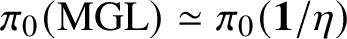
is equivalent to the profinite completion of a circle. That is, up to completion, (1.1) can be expressed more suggestively as
$(\mathbb {F}_p)_{\acute {e}t} \simeq (\mathbb {Z}_p)_{\acute {e}t}$
is equivalent to the profinite completion of a circle. That is, up to completion, (1.1) can be expressed more suggestively as
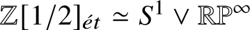 $\mathbb {Z}[1/2]_{\acute {e}t} \simeq S^1 \vee \mathbb R\mathbb P^\infty $
. For our generalisation to stable motivic homotopy invariants, it will be essential to keep track of the fields and not just their étale homotopy types.
$\mathbb {Z}[1/2]_{\acute {e}t} \simeq S^1 \vee \mathbb R\mathbb P^\infty $
. For our generalisation to stable motivic homotopy invariants, it will be essential to keep track of the fields and not just their étale homotopy types.
The presentation of
 $\mathbb {Z}[1/2]_{\acute {e}t}^\wedge $
has powerful consequences; for example, taking the
$\mathbb {Z}[1/2]_{\acute {e}t}^\wedge $
has powerful consequences; for example, taking the
 $2$
-adic étale K-theory of (1.1) yields a pullback square. Combined with the Quillen–Lichtenbaum conjecture for the 2-primary algebraic K-theory of
$2$
-adic étale K-theory of (1.1) yields a pullback square. Combined with the Quillen–Lichtenbaum conjecture for the 2-primary algebraic K-theory of
 $\mathbb {Z}[1/2]$
(see [Reference Østvær17], [Reference Dugger and Isaksen74], [Reference Gras58], [Reference Bousfield34]), one obtains the pullback square
$\mathbb {Z}[1/2]$
(see [Reference Østvær17], [Reference Dugger and Isaksen74], [Reference Gras58], [Reference Bousfield34]), one obtains the pullback square

We show that replacing algebraic K-theory in (1.2) by an arbitrary cellular motivic spectrum over
 $\mathbb {Z}[1/2]$
still yields a pullback square. Let
$\mathbb {Z}[1/2]$
still yields a pullback square. Let
 $\mathcal {SH}(X)$
denote the motivic stable homotopy category of X; see [Reference Bachmann42], [Reference Bachmann and Hoyois22], [Reference Pstrągowski54, §5], [Reference Friedlander11, §4.1]. We write
$\mathcal {SH}(X)$
denote the motivic stable homotopy category of X; see [Reference Bachmann42], [Reference Bachmann and Hoyois22], [Reference Pstrągowski54, §5], [Reference Friedlander11, §4.1]. We write
 $\mathcal {SH}(X)^{\text {cell}} \subset \mathcal {SH}(X)$
for the full subcategory of cellular motivic spectra [Reference Dundas, Röndigs and Østvær20]; that is, the localising subcategory generated by the bigraded spheres
$\mathcal {SH}(X)^{\text {cell}} \subset \mathcal {SH}(X)$
for the full subcategory of cellular motivic spectra [Reference Dundas, Röndigs and Østvær20]; that is, the localising subcategory generated by the bigraded spheres
 $S^{p,q}$
for all integers
$S^{p,q}$
for all integers
 $p,q\in \mathbb {Z}$
. For simplicity we state a special case of Theorem 4.7; see Example 4.10.
$p,q\in \mathbb {Z}$
. For simplicity we state a special case of Theorem 4.7; see Example 4.10.
Theorem 1.2. For every
 $\mathcal {E} \in \mathcal {SH}(\mathbb {Z}[1/2])^{\text {cell}}$
there is a pullback square
$\mathcal {E} \in \mathcal {SH}(\mathbb {Z}[1/2])^{\text {cell}}$
there is a pullback square

Here, for
 $X \in \mathrm {S}\mathrm {ch}{}_{\mathbb {Z}[1/2]}$
, we denote by
$X \in \mathrm {S}\mathrm {ch}{}_{\mathbb {Z}[1/2]}$
, we denote by
 $\mathcal {E}(X)$
the (ordinary) spectrum of maps from
$\mathcal {E}(X)$
the (ordinary) spectrum of maps from
 $\mathbf {1}_X$
to
$\mathbf {1}_X$
to
 $p^*\mathcal {E}$
in
$p^*\mathcal {E}$
in
 $\mathcal {SH}(X)$
, where
$\mathcal {SH}(X)$
, where
 $\mathbf {1}_X \in \mathcal {SH}(X)$
denotes the unit object and
$\mathbf {1}_X \in \mathcal {SH}(X)$
denotes the unit object and
 $p: X \to \mathbb {Z}[1/2]$
is the structure map.
$p: X \to \mathbb {Z}[1/2]$
is the structure map.
Example 1.3. The motivic spectra representing algebraic K-theory,
 $\mathrm {KGL}$
, hermitian K-theory,
$\mathrm {KGL}$
, hermitian K-theory,
 $\mathrm {KO}$
, Witt-theory,
$\mathrm {KO}$
, Witt-theory,
 $\mathrm {KW}$
, motivic cohomology or higher Chow groups,
$\mathrm {KW}$
, motivic cohomology or higher Chow groups,
 $\mathrm {H}\mathbb {Z}$
, and algebraic cobordism,
$\mathrm {H}\mathbb {Z}$
, and algebraic cobordism,
 $\mathrm {MGL}$
, are cellular (at least after localisation at
$\mathrm {MGL}$
, are cellular (at least after localisation at
 $2$
) by respectively [Reference Dundas, Röndigs and Østvær20, Theorem 6.2], [Reference Siegel62, Theorem 1], [Reference Lurie36, Proposition 8.1] and [Reference Röndigs, Spitzweck and Østvær69, Corollary 10.4], [Reference Dundas, Röndigs and Østvær20, Theorem 6.4]. We refer to [Reference Artin and Mazur10, Proposition 8.12] for cellularity of the corresponding (very effective or connective) covers
$2$
) by respectively [Reference Dundas, Röndigs and Østvær20, Theorem 6.2], [Reference Siegel62, Theorem 1], [Reference Lurie36, Proposition 8.1] and [Reference Röndigs, Spitzweck and Østvær69, Corollary 10.4], [Reference Dundas, Röndigs and Østvær20, Theorem 6.4]. We refer to [Reference Artin and Mazur10, Proposition 8.12] for cellularity of the corresponding (very effective or connective) covers
 $\mathrm {kgl}$
,
$\mathrm {kgl}$
,
 $\mathrm {ko}$
,
$\mathrm {ko}$
,
 $\mathrm {kw}$
, in the sense of [Reference Lam70] and Milnor-Witt motivic cohomology
$\mathrm {kw}$
, in the sense of [Reference Lam70] and Milnor-Witt motivic cohomology
 $\mathrm {H}\widetilde {\mathbb {Z}}$
, in the sense of [Reference Isaksen and Østvær8], [Reference Elmanto and Shah6].
$\mathrm {H}\widetilde {\mathbb {Z}}$
, in the sense of [Reference Isaksen and Østvær8], [Reference Elmanto and Shah6].
In the case of
 $\mathcal {E}=\mathrm {KGL}$
, Theorem 1.2 recovers the stable version of [Reference Bousfield34, Theorem 1.1], and for
$\mathcal {E}=\mathrm {KGL}$
, Theorem 1.2 recovers the stable version of [Reference Bousfield34, Theorem 1.1], and for
 $\mathcal {E}=\mathrm {KO}$
it recovers [Reference Bökstedt15, Theorem 1.1] (in fact, we extend these results to arbitrary
$\mathcal {E}=\mathrm {KO}$
it recovers [Reference Bökstedt15, Theorem 1.1] (in fact, we extend these results to arbitrary
 $2$
-regular number fields, not necessarily totally real). The squares for
$2$
-regular number fields, not necessarily totally real). The squares for
 $\mathrm {KW}$
,
$\mathrm {KW}$
,
 $\mathrm {H}\mathbb {Z}$
,
$\mathrm {H}\mathbb {Z}$
,
 $\mathrm {H}\widetilde {\mathbb {Z}}$
,
$\mathrm {H}\widetilde {\mathbb {Z}}$
,
 $\mathrm {MGL}$
,
$\mathrm {MGL}$
,
 $\mathrm {kgl}$
,
$\mathrm {kgl}$
,
 $\mathrm {ko}$
,
$\mathrm {ko}$
,
 $\mathrm {kw}$
appear to be new.
$\mathrm {kw}$
appear to be new.
A striking application of Theorem 1.2 is that it relates the universal motivic invariants over
 $\mathbb {Z}[1/2]$
to the same invariants over
$\mathbb {Z}[1/2]$
to the same invariants over
 $\mathbb C$
,
$\mathbb C$
,
 $\mathbb R$
and
$\mathbb R$
and
 $\mathbb {F}_{3}$
. That is, applying (1.3) to the motivic sphere
$\mathbb {F}_{3}$
. That is, applying (1.3) to the motivic sphere
 $\mathcal {E}=\mathbf {1}_{\mathbb {Z}[1/2]}$
enables computations of the stable motivic homotopy groups of
$\mathcal {E}=\mathbf {1}_{\mathbb {Z}[1/2]}$
enables computations of the stable motivic homotopy groups of
 $\mathbb {Z}[1/2]$
. We identify, up to odd-primary torsion, the endomorphism ring of
$\mathbb {Z}[1/2]$
. We identify, up to odd-primary torsion, the endomorphism ring of
 $\mathbf {1}_{\mathbb {Z}[1/2]}$
with the Grothendieck–Witt ring of quadratic forms of the Dedekind domain
$\mathbf {1}_{\mathbb {Z}[1/2]}$
with the Grothendieck–Witt ring of quadratic forms of the Dedekind domain
 $\mathbb {Z}[1/2]$
defined in [Reference Bachmann, Elmanto and Østvær53, Chapter IV, §3]. This extends Morel’s fundamental computation of
$\mathbb {Z}[1/2]$
defined in [Reference Bachmann, Elmanto and Østvær53, Chapter IV, §3]. This extends Morel’s fundamental computation of
 $\pi _{0,0}(\mathbf {1})$
over fields [Reference Pstrągowski54, §6] to an arithmetic situation.
$\pi _{0,0}(\mathbf {1})$
over fields [Reference Pstrągowski54, §6] to an arithmetic situation.
Theorem 1.4. The unit map
 $\mathbf {1}_{\mathbb {Z}[1/2]} \to \mathrm {KO}_{\mathbb {Z}[1/2]}$
induces an isomorphism
$\mathbf {1}_{\mathbb {Z}[1/2]} \to \mathrm {KO}_{\mathbb {Z}[1/2]}$
induces an isomorphism
 $$ \begin{align*} \pi_{0,0}(\mathbf{1}_{\mathbb{Z}[1/2]}) \otimes \mathbb{Z}_{(2)} \cong \mathrm{GW}(\mathbb{Z}[1/2]) \otimes \mathbb{Z}_{(2)}. \end{align*} $$
Remark 1.5. The étale homotopy types of various other rings and applications to algebraic K-theory and group homology of general linear groups were worked out in [Reference Dugger and Isaksen23], [Reference Röndigs, Spitzweck and Østvær24], [Reference Neukirch57], [Reference Bousfield34]. We show similar generalisations of (1.3) with
 $\mathbb {Z}[1/2]$
replaced by
$\mathbb {Z}[1/2]$
replaced by
 $\mathcal O_F[1/2]$
, for F any
$\mathcal O_F[1/2]$
, for F any
 $2$
-regular number field, or by
$2$
-regular number field, or by
 $\mathbb {Z}[1/\ell ]$
,
$\mathbb {Z}[1/\ell ]$
,
 $\mathbb {Z}[1/\ell ,\zeta _\ell ]$
, where
$\mathbb {Z}[1/\ell ,\zeta _\ell ]$
, where
 $\ell $
is an odd regular prime and
$\ell $
is an odd regular prime and
 $\zeta _\ell $
is a primitive
$\zeta _\ell $
is a primitive
 $\ell $
th root of unity; to achieve this, we slightly alter the other terms in (1.3). See Theorems 4.7, 4.11, 4.14, 5.2 for precise statements.
$\ell $
th root of unity; to achieve this, we slightly alter the other terms in (1.3). See Theorems 4.7, 4.11, 4.14, 5.2 for precise statements.
Another application, which will be explored elsewhere, is the spherical Quillen–Lichtenbaum property saying the canonical map from stable motivic homotopy groups to stable étale motivic homotopy groups is an isomorphism in certain degrees. Slice completeness is an essential input for showing the spherical property; we deduce this for base schemes such as
 $\mathbb {Z}[1/2]$
in Proposition 11.
$\mathbb {Z}[1/2]$
in Proposition 11.
As a final comment, we expect that most of the applications we establish hold over more general base schemes, where convenient reductions to small fields are not possible. The proofs will require significantly different ideas.
Organisation
In Section 2 we give proofs for some more or less standard facts about nilpotent completions in stable
 $\infty $
-categories with t-structures. While these results are relatively straightforward generalisations of Bousfield’s pioneering work [Reference Hodgkin and Østvær18], we could not locate a reference in the required generality. These nilpotent completions will be our primary tool throughout the rest of the article. In Section 3 we prove a variant of Gabber rigidity. We show that, for example, if
$\infty $
-categories with t-structures. While these results are relatively straightforward generalisations of Bousfield’s pioneering work [Reference Hodgkin and Østvær18], we could not locate a reference in the required generality. These nilpotent completions will be our primary tool throughout the rest of the article. In Section 3 we prove a variant of Gabber rigidity. We show that, for example, if
 $E \in \mathcal {SH}(X)^{\text {cell}}$
where X is essentially smooth over a Dedekind scheme, then
$E \in \mathcal {SH}(X)^{\text {cell}}$
where X is essentially smooth over a Dedekind scheme, then
 $E(X_x^h)_\ell ^\wedge \simeq E(x)_\ell ^\wedge $
for any point
$E(X_x^h)_\ell ^\wedge \simeq E(x)_\ell ^\wedge $
for any point
 $x \in X$
such that
$x \in X$
such that
 $\ell $
is invertible in
$\ell $
is invertible in
 $k(x)$
. Here
$k(x)$
. Here
 $X_x^h$
denotes the henselisation of X along x. Our principal results are shown in Section 4. We establish a general method for exhibiting squares as above and provide a criterion for cartesianess in terms of étale and real étale cohomology; see Proposition 7. Next we verify this criterion for regular number rings, reducing essentially to global class field theory – which is also how Dwyer–Friedlander established (1.1). In Section 5 we discuss some applications, including a proof of Theorem 1.4.
$X_x^h$
denotes the henselisation of X along x. Our principal results are shown in Section 4. We establish a general method for exhibiting squares as above and provide a criterion for cartesianess in terms of étale and real étale cohomology; see Proposition 7. Next we verify this criterion for regular number rings, reducing essentially to global class field theory – which is also how Dwyer–Friedlander established (1.1). In Section 5 we discuss some applications, including a proof of Theorem 1.4.
Notation and conventions
We freely use the language of (stable) infinity categories, as set out in [Reference Scheiderer48, Reference Andradas, Bröcker and Ruiz49]. Given a (stable)
 $\infty $
-category
$\infty $
-category
 $\mathcal C$
and objects
$\mathcal C$
and objects
 $c, d \in \mathcal C$
, we denote by
$c, d \in \mathcal C$
, we denote by
 $\mathrm {Map}(c,d) = \mathrm {Map}_{\mathcal C}(c,d)$
(respectively
$\mathrm {Map}(c,d) = \mathrm {Map}_{\mathcal C}(c,d)$
(respectively
 $\mathrm {map}(c,d) = \mathrm {map}_{\mathcal {C}}(c,d)$
) the mapping space (respectively mapping spectrum). Given a symmetric monoidal category
$\mathrm {map}(c,d) = \mathrm {map}_{\mathcal {C}}(c,d)$
) the mapping space (respectively mapping spectrum). Given a symmetric monoidal category
 $\mathcal C$
, we denote the unit object by
$\mathcal C$
, we denote the unit object by
 $\mathbf {1} = \mathbf {1}_{\mathcal {C}}$
. We assume familiarity with the motivic stable category
$\mathbf {1} = \mathbf {1}_{\mathcal {C}}$
. We assume familiarity with the motivic stable category
 $\mathcal {SH}(S)$
; see, for example, [Reference Friedlander11, §4.1]. We write
$\mathcal {SH}(S)$
; see, for example, [Reference Friedlander11, §4.1]. We write
 $\Sigma ^{p,q} = \Sigma ^{p-q} \wedge {\mathbb {G}_m^{\wedge q}}$
for the bigraded suspension functor and
$\Sigma ^{p,q} = \Sigma ^{p-q} \wedge {\mathbb {G}_m^{\wedge q}}$
for the bigraded suspension functor and
 $S^{p,q} = \Sigma ^{p,q} \mathbf {1}$
for the bigraded spheres.
$S^{p,q} = \Sigma ^{p,q} \mathbf {1}$
for the bigraded spheres.
2 Nilpotent completions
We axiomatise some well-known facts about nilpotent completions in presentably symmetric monoidal stable
 $\infty $
-categories with a t-structure. Our arguments are straightforward generalisations of [Reference Hodgkin and Østvær18] and [Reference Druzhinin50]. Theorems 2.1 and 2.2 are the main results in this section.
$\infty $
-categories with a t-structure. Our arguments are straightforward generalisations of [Reference Hodgkin and Østvær18] and [Reference Druzhinin50]. Theorems 2.1 and 2.2 are the main results in this section.
2.1 Overview
Throughout we let
 $\mathcal C$
be a presentably symmetric monoidal
$\mathcal C$
be a presentably symmetric monoidal
 $\infty $
-category (i.e., the tensor product preserves colimits in each variable separately) provided with a t-structure which is compatible with the symmetric monoidal structure (i.e.,
$\infty $
-category (i.e., the tensor product preserves colimits in each variable separately) provided with a t-structure which is compatible with the symmetric monoidal structure (i.e.,
 $\mathcal C_{\ge 0} \otimes \mathcal C_{\ge 0} \subset \mathcal C_{\ge 0}$
) and weakly left complete, by which we mean that for
$\mathcal C_{\ge 0} \otimes \mathcal C_{\ge 0} \subset \mathcal C_{\ge 0}$
) and weakly left complete, by which we mean that for
 $X \in \mathcal C$
we have
$X \in \mathcal C$
we have
 $X \simeq \operatorname *{\mathrm {lim}}_n X_{\le n}$
. Given
$X \simeq \operatorname *{\mathrm {lim}}_n X_{\le n}$
. Given
 $E \in \mathrm {CAlg}(\mathcal C)$
and
$E \in \mathrm {CAlg}(\mathcal C)$
and
 $X \in \mathcal C$
, recall [51, Construction 2.7] the standard cosimplicial resolution (or cobar construction)
$X \in \mathcal C$
, recall [51, Construction 2.7] the standard cosimplicial resolution (or cobar construction)
 $$ \begin{align*} \Delta_+ \to \mathcal C, [n] \mapsto X \otimes E^{\otimes n+1} \end{align*} $$
whose limit is (for us by definition) the E-nilpotent completion
 $X_E^\wedge $
.
$X_E^\wedge $
.
We call
 $X \in \mathcal C$
bounded below if
$X \in \mathcal C$
bounded below if
 $X \in \cup _n \mathcal C_{\ge n}$
. Recall that
$X \in \cup _n \mathcal C_{\ge n}$
. Recall that
 $R \in \mathrm {CAlg}(\mathcal C^\heartsuit )$
is called idempotent if the multiplication map
$R \in \mathrm {CAlg}(\mathcal C^\heartsuit )$
is called idempotent if the multiplication map
 $R \otimes ^\heartsuit R \to R \in \mathcal C^\heartsuit $
is an equivalence.
$R \otimes ^\heartsuit R \to R \in \mathcal C^\heartsuit $
is an equivalence.
Theorem 2.1. Let
 $\mathcal C$
be weakly left complete,
$\mathcal C$
be weakly left complete,
 $E \in \mathrm {CAlg}(\mathcal C_{\ge 0})$
and
$E \in \mathrm {CAlg}(\mathcal C_{\ge 0})$
and
 $X \in \mathcal C$
. Suppose that
$X \in \mathcal C$
. Suppose that
 $\pi _0 E \in \mathrm {CAlg}(\mathcal C^\heartsuit )$
is idempotent and X is bounded below. Then the canonical map
$\pi _0 E \in \mathrm {CAlg}(\mathcal C^\heartsuit )$
is idempotent and X is bounded below. Then the canonical map
 $$ \begin{align*} X_E^\wedge \to X_{\pi_0 E}^\wedge \end{align*} $$
is an equivalence.
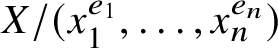
One way of producing idempotent algebras is by taking quotients of the unit. Given
 $L_1, \dots , L_n \in \mathcal C_{\ge 0}$
and maps
$L_1, \dots , L_n \in \mathcal C_{\ge 0}$
and maps
 $x_i: L_i \to \mathbf {1}$
, we set
$x_i: L_i \to \mathbf {1}$
, we set
 $$ \begin{align*} X/(x_1^{m_1}, x_2^{m_2}, \dots, x_n^{m_n}) = X \otimes \mathrm{cof}(x_n^{\otimes m_n}: L_n^{\otimes m_n} \to 1) \otimes \dots \otimes \mathrm{cof}(x_1^{\otimes m_1}: L_1^{\otimes m_1} \to 1). \end{align*} $$
The object
 $\pi _0(\mathbf {1}/(x_1, \dots , x_n)) \in \mathrm {CAlg}(\mathcal C^\heartsuit )$
is idempotent. For varying m, the
$\pi _0(\mathbf {1}/(x_1, \dots , x_n)) \in \mathrm {CAlg}(\mathcal C^\heartsuit )$
is idempotent. For varying m, the
 $\mathbf {1}/x_i^m$
s form an inverse system indexed on
$\mathbf {1}/x_i^m$
s form an inverse system indexed on
 $\mathbb {N}$
in an evident way; by taking tensor products, the objects
$\mathbb {N}$
in an evident way; by taking tensor products, the objects
 $X/(x_1^{m_1}, \dots , x_n^{m_n})$
form an
$X/(x_1^{m_1}, \dots , x_n^{m_n})$
form an
 $\mathbb {N}^n$
-indexed inverse system. We define the x-completion of X as the limit
$\mathbb {N}^n$
-indexed inverse system. We define the x-completion of X as the limit
 $$ \begin{align*} X_{x_1, \dots, x_n}^\wedge := \operatorname*{\mathrm{lim}}_{m_1, \dots, m_n} X/(x_1^{m_1}, \dots, x_n^{m_n}). \end{align*} $$
Theorem 2.2. Suppose each
 $L_i\in \mathcal C_{\ge 0}$
is strongly dualisable with dual
$L_i\in \mathcal C_{\ge 0}$
is strongly dualisable with dual
 $DL_i \in \mathcal C_{\ge 0}$
. If
$DL_i \in \mathcal C_{\ge 0}$
. If
 $X \in \mathcal C$
is bounded below and
$X \in \mathcal C$
is bounded below and
 $\mathcal C$
is weakly left complete, then there is a canonical equivalence
$\mathcal C$
is weakly left complete, then there is a canonical equivalence
 $$ \begin{align*} X_{\pi_0(\mathbf{1}/(x_1, \dots, x_n))}^\wedge \simeq X_{x_1, \dots, x_n}^\wedge. \end{align*} $$
To apply Theorem 2.2 in motivic stable homotopy theory we consider, for a scheme S, the homotopy t-structure on
 $\mathcal {SH}(S)$
; see, for example, [Reference Friedlander11, §B], [Reference Röndigs and Østvær66, §1].
$\mathcal {SH}(S)$
; see, for example, [Reference Friedlander11, §B], [Reference Röndigs and Østvær66, §1].
Theorem 2.3. Let S be a noetherian scheme of finite Krull dimension and suppose
 $X \in \mathcal {SH}(S)$
is bounded below.
$X \in \mathcal {SH}(S)$
is bounded below.
-
1. There is an equivalence
 $X_{\mathrm {MGL}}^\wedge \simeq X_\eta ^\wedge $
.
$X_{\mathrm {MGL}}^\wedge \simeq X_\eta ^\wedge $
. -
2. If
$1/\ell \in S$
, then there is an equivalence
$X_{H\mathbb {F}_\ell }^\wedge \simeq X_{\eta ,\ell }^\wedge $
.
Proof. The homotopy t-structure is weakly left complete by [Reference Röndigs and Østvær66, Corollary 3.8].
(1) Owing to [Reference Lurie36, Theorem 3.8, Corollary 3.9] we have
 $\mathrm {MGL} \in \mathcal {SH}(S)_{\ge 0}$
and
$\mathrm {MGL} \in \mathcal {SH}(S)_{\ge 0}$
and
 $\pi _0(\mathrm {MGL}) \simeq \pi _0(\mathbf {1}/\eta )$
.
$\pi _0(\mathrm {MGL}) \simeq \pi _0(\mathbf {1}/\eta )$
.
(2) We need to prove that
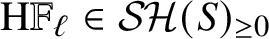 $\mathrm {H}\mathbb {F}_\ell \in \mathcal {SH}(S)_{\ge 0}$
and
$\mathrm {H}\mathbb {F}_\ell \in \mathcal {SH}(S)_{\ge 0}$
and
 $\pi _0(\mathrm {H}\mathbb {F}_\ell ) \simeq \pi _0(\mathbf {1}/(\eta ,\ell ))$
. Since
$\pi _0(\mathrm {H}\mathbb {F}_\ell ) \simeq \pi _0(\mathbf {1}/(\eta ,\ell ))$
. Since
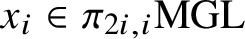 $x_i\in \pi _{2i,i}\mathrm {MGL}$
and
$x_i\in \pi _{2i,i}\mathrm {MGL}$
and
 $\Sigma ^{2i,i}\mathrm {MGL}=\Sigma ^i{\mathbb {G}_m^{\wedge i}}\wedge \mathrm {MGL}\in \mathcal {SH}(S)_{\ge i}\subset \mathcal {SH}(S)_{>0}$
, both of these claims follow from the Hopkins–Morel isomorphism
$\Sigma ^{2i,i}\mathrm {MGL}=\Sigma ^i{\mathbb {G}_m^{\wedge i}}\wedge \mathrm {MGL}\in \mathcal {SH}(S)_{\ge i}\subset \mathcal {SH}(S)_{>0}$
, both of these claims follow from the Hopkins–Morel isomorphism
 $$ \begin{align*} \mathrm{H}\mathbb{F}_\ell \simeq \mathrm{MGL}/(\ell, x_1, x_2, \dots) \end{align*} $$
shown in [Reference Röndigs, Spitzweck and Østvær69, Theorem 10.3].Footnote 1
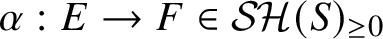
Remark 2.4. Theorem 2.3 implies that a map
 $\alpha : E \to F \in \mathcal {SH}(S)_{\ge 0}$
is an
$\alpha : E \to F \in \mathcal {SH}(S)_{\ge 0}$
is an
 $(\eta ,\ell )$
-adic equivalence if and only if
$(\eta ,\ell )$
-adic equivalence if and only if
 $\alpha \wedge \mathrm {H}\mathbb {F}_\ell $
is an equivalence, which is also easily seen by considering homotopy objects. This weaker statement, however, cannot be used as a replacement for Theorem 2.3 in this work.
$\alpha \wedge \mathrm {H}\mathbb {F}_\ell $
is an equivalence, which is also easily seen by considering homotopy objects. This weaker statement, however, cannot be used as a replacement for Theorem 2.3 in this work.
2.2 Proofs
Recall that
 $\mathcal C$
is a presentably symmetric monoidal
$\mathcal C$
is a presentably symmetric monoidal
 $\infty $
-category equipped with a compatible t-structure.
$\infty $
-category equipped with a compatible t-structure.
Definition 1.
-
1. Let
$E \in \mathrm {CAlg}(\mathcal C)$
. Then
$X \in \mathcal C$
is E-nilpotent if it lies in the thick subcategory generated by objects of the form
$E \otimes Y$
for
$Y \in \mathcal C$
. -
2. Let
$R \in \mathrm {CAlg}(\mathcal C^\heartsuit )$
be idempotent. Then
$F \in \mathcal C^\heartsuit $
is strongly R-nilpotent if F admits a finite filtration whose subquotients are R-modules.Footnote
2
Moreover,
$X \in \mathcal C$
is strongly R-nilpotent if it is bounded in the t-structure and all homotopy objects are strongly R-nilpotent.


Example 2.5. If
 $X \in \mathcal C$
is an E-module in the homotopy category, then it is a summand of
$X \in \mathcal C$
is an E-module in the homotopy category, then it is a summand of
 $X \otimes E$
and thus X is E-nilpotent.
$X \otimes E$
and thus X is E-nilpotent.
Lemma 2.6. Suppose
 $R \in \mathrm {CAlg}(\mathcal C^\heartsuit )$
is idempotent.
$R \in \mathrm {CAlg}(\mathcal C^\heartsuit )$
is idempotent.
-
1. Let
be an exact sequence. If
$$ \begin{align*} A \to B \to C \to D \to E \in \mathcal C^\heartsuit \end{align*} $$
$A,B,D,E$
are strongly R-nilpotent, then so is
$\mathcal C$
.
-
2. An object
$X \in \mathcal C$
is strongly R-nilpotent if and only if it is R-nilpotent and bounded in the t-structure.


Proof. (1) The proofs of [Reference Druzhinin50, Lemmas 7.2.7–7.2.9] apply unchanged. (2) Example 2.5 implies that strongly R-nilpotent objects are R-nilpotent, being finite extensions of homotopy R-modules. It thus suffices to show that if X is R-nilpotent, then its homotopy objects
 $\pi _i^{\mathcal C}(X) \in \mathcal C^\heartsuit $
are strongly R-nilpotent. This is clear for free R-modules, and the property is preserved by taking summands and shifts and cofibres by (1). The result follows.
$\pi _i^{\mathcal C}(X) \in \mathcal C^\heartsuit $
are strongly R-nilpotent. This is clear for free R-modules, and the property is preserved by taking summands and shifts and cofibres by (1). The result follows.
Definition 2.
-
1. If
$E \in \mathrm {CAlg}(\mathcal C)$
,
$X \in \mathcal C$
, a tower of the form is called an E-nilpotent resolution if each
$$ \begin{align*} X \to \dots \to X_2 \to X_1 \to X_0 \end{align*} $$
$X_i$
is E-nilpotent and for every E-nilpotent
$Y \in \mathcal C$
, we have
$$ \begin{align*} \operatorname*{\mathrm{colim}}_n [X_n, Y] \xrightarrow{\simeq} [X, Y]. \end{align*} $$
-
2. If
$R \in \mathrm {CAlg}(\mathcal C^\heartsuit )$
is idempotent and
$X \in \mathcal C$
, a tower of the form is called a strongly R-nilpotent resolution if each
$$ \begin{align*} X \to \dots \to X_2 \to X_1 \to X_0 \end{align*} $$
$X_i$
is strongly R-nilpotent and for every strongly R-nilpotent
$Y \in \mathcal C$
, we have
$$ \begin{align*} \operatorname*{\mathrm{colim}}_n [X_n, Y] \xrightarrow{\simeq} [X, Y]. \end{align*} $$


Proposition 3. For
 $X, Y \in \mathcal C$
and
$X, Y \in \mathcal C$
and
 $X_\bullet , Y_\bullet E$
-nilpotent (respectively strongly R-nilpotent) resolutions, we have
$X_\bullet , Y_\bullet E$
-nilpotent (respectively strongly R-nilpotent) resolutions, we have
 $$ \begin{align*} \mathrm{Map}_{\mathrm{Pro}(\mathcal C)}(X_\bullet, Y_\bullet) \simeq \operatorname*{\mathrm{lim}}_n \mathrm{Map}(X, Y_\bullet). \end{align*} $$
Thus, any map
 $X \to Y$
induces a canonical morphism of towers
$X \to Y$
induces a canonical morphism of towers
 $X_\bullet \to Y_\bullet $
. In particular, if
$X_\bullet \to Y_\bullet $
. In particular, if
 $X \simeq Y$
, then
$X \simeq Y$
, then
 $X_\bullet \simeq Y_\bullet \in \mathrm {Pro}(\mathcal C)$
and
$X_\bullet \simeq Y_\bullet \in \mathrm {Pro}(\mathcal C)$
and
 $\operatorname *{\mathrm {lim}}_n X_n \simeq \operatorname *{\mathrm {lim}}_n Y_n$
.
$\operatorname *{\mathrm {lim}}_n X_n \simeq \operatorname *{\mathrm {lim}}_n Y_n$
.
Proof. Essentially, by definition we have
 $$ \begin{align*} \mathrm{Map}(X_\bullet, Y_\bullet) \simeq \operatorname*{\mathrm{lim}}_n\ \operatorname*{\mathrm{colim}}_m\ \mathrm{Map}(X_m, Y_n). \end{align*} $$
The colimit is equivalent to
 $\mathrm {Map}(X, Y_n)$
by the definition of a resolution.
$\mathrm {Map}(X, Y_n)$
by the definition of a resolution.
Lemma 2.7. Let
 $E \in \mathrm {CAlg}(\mathcal C)$
and
$E \in \mathrm {CAlg}(\mathcal C)$
and
 $X \in \mathcal C$
.
$X \in \mathcal C$
.
-
1. The tower of partial totalisations of the standard cosimplicial objects
$X \otimes E^{\otimes \bullet }$
is an E-nilpotent resolution of X. -
2. Suppose that
$E \in \mathcal C_{\ge 0}$
and
$\pi _0 E$
is idempotent. Then if
$X \to X_\bullet $
is any E-nilpotent resolution by bounded below objects (e.g., if X is bounded below, the one arising from (1)), then
$X \to \tau _{\le \bullet } X_\bullet $
is a strongly
$\pi _0(E)$
-nilpotent resolution.


Proof. (1) Since partial totalisations are finite limits, they commute with
 $\otimes X$
, by stability, and are thus given by
$\otimes X$
, by stability, and are thus given by
 $X_i = X \otimes \mathrm {cof}(I^{\otimes i} \to \mathbf {1})$
, where
$X_i = X \otimes \mathrm {cof}(I^{\otimes i} \to \mathbf {1})$
, where
 $I = \mathrm {fib}(\mathbf {1} \to E)$
, see [51, Proposition 2.14]. In the notation of loc. cit. we get
$I = \mathrm {fib}(\mathbf {1} \to E)$
, see [51, Proposition 2.14]. In the notation of loc. cit. we get
 $\mathrm {cof}(X_i \to X_{i-1}) \simeq \Sigma \mathrm {cof}(T_i(E, X) \to T_{i-1}(E, X))$
and
$\mathrm {cof}(X_i \to X_{i-1}) \simeq \Sigma \mathrm {cof}(T_i(E, X) \to T_{i-1}(E, X))$
and
 $X_0 = 0$
. This implies
$X_0 = 0$
. This implies
 $X_i$
is E-nilpotent by [51, Proposition 2.5(1)]. To conclude, it suffices to prove that if Y is E-nilpotent, then
$X_i$
is E-nilpotent by [51, Proposition 2.5(1)]. To conclude, it suffices to prove that if Y is E-nilpotent, then
 $\operatorname *{\mathrm {colim}}_i\, \mathrm {map}(X_i, Y) \simeq \mathrm {map}(X, Y)$
. The class of objects Y satisfying the latter equivalence is thick, so we may assume that Y is an E-module. We are reduced to proving that
$\operatorname *{\mathrm {colim}}_i\, \mathrm {map}(X_i, Y) \simeq \mathrm {map}(X, Y)$
. The class of objects Y satisfying the latter equivalence is thick, so we may assume that Y is an E-module. We are reduced to proving that
 $\operatorname *{\mathrm {colim}}_i\, \mathrm {map}(I^{\otimes i} \otimes X, Y) = 0$
. But this is a summand of
$\operatorname *{\mathrm {colim}}_i\, \mathrm {map}(I^{\otimes i} \otimes X, Y) = 0$
. But this is a summand of
 $\operatorname *{\mathrm {colim}}_i\, \mathrm {map}(I^{\otimes i} \otimes X \otimes E, Y)$
, Y being an E-module, and the transition maps
$\operatorname *{\mathrm {colim}}_i\, \mathrm {map}(I^{\otimes i} \otimes X \otimes E, Y)$
, Y being an E-module, and the transition maps
 $I^{\otimes i+1} \otimes E \to I^{\otimes i} \otimes E$
are null by [51, Proposition 2.5(2)], so the colimit vanishes as desired.
$I^{\otimes i+1} \otimes E \to I^{\otimes i} \otimes E$
are null by [51, Proposition 2.5(2)], so the colimit vanishes as desired.
(2) We first show that each
 $\tau _{\le n} X_n$
is strongly R-nilpotent and, more generally, that if Y is E-nilpotent, then each
$\tau _{\le n} X_n$
is strongly R-nilpotent and, more generally, that if Y is E-nilpotent, then each
 $\pi _i(Y)$
is strongly R-nilpotent. By Lemma 2.6(1) we may assume Y is a (free) E-module; in this case, each
$\pi _i(Y)$
is strongly R-nilpotent. By Lemma 2.6(1) we may assume Y is a (free) E-module; in this case, each
 $\pi _i(Y)$
is a
$\pi _i(Y)$
is a
 $\pi _0(E)$
-module. Suppose
$\pi _0(E)$
-module. Suppose
 $Y \in \mathcal C$
is strongly
$Y \in \mathcal C$
is strongly
 $\pi _0(E)$
-nilpotent. Then Y is E-nilpotent since any
$\pi _0(E)$
-nilpotent. Then Y is E-nilpotent since any
 $\pi _0(E)$
-module is an E-module. Finally, we have
$\pi _0(E)$
-module is an E-module. Finally, we have
 $$ \begin{align*} \operatorname*{\mathrm{colim}}_n [\tau_{\le n} X_n, Y] \simeq \operatorname*{\mathrm{colim}}_n [X_n, Y] \simeq [X, Y]. \end{align*} $$
Here the first equivalence holds since Y is bounded above and the second because Y is E-nilpotent.
Next we prove that the E-nilpotent completion only depends on
 $\pi _0(E)$
.
$\pi _0(E)$
.
Proof of Theorem 2.1. For
 $E \in \mathrm {CAlg}(\mathcal C_{\ge 0})$
and
$E \in \mathrm {CAlg}(\mathcal C_{\ge 0})$
and
 $X \in \mathcal C$
, denote by
$X \in \mathcal C$
, denote by
 $R_n(E, X)$
the nth partial totalisation of
$R_n(E, X)$
the nth partial totalisation of
 $X \otimes E^{\otimes \bullet }$
, so that
$X \otimes E^{\otimes \bullet }$
, so that
 $X \to R_\bullet (E, X)$
is a tower with limit
$X \to R_\bullet (E, X)$
is a tower with limit
 $X \to X_E^\wedge $
. By left completeness and cofinality we have
$X \to X_E^\wedge $
. By left completeness and cofinality we have
 $$ \begin{align*} X_E^\wedge \simeq \operatorname*{\mathrm{lim}}_{m,n} \tau_{\le m} R_n(X, E) \simeq \operatorname*{\mathrm{lim}}_n \tau_{\le n} R_n(X, E). \end{align*} $$
By Lemma 2.7, the right-hand side is the limit of a strongly
 $\pi _0(E)$
-nilpotent resolution, which by Proposition 3 only depends on X and
$\pi _0(E)$
-nilpotent resolution, which by Proposition 3 only depends on X and
 $\pi _0(E)$
.
$\pi _0(E)$
.
Remark 2.8. The proof also verifies that any strongly
 $\pi _0(E)$
-nilpotent resolution of X has limit
$\pi _0(E)$
-nilpotent resolution of X has limit
 $X_{\pi _0 E}^\wedge $
.
$X_{\pi _0 E}^\wedge $
.
We now turn to the study of x-completions.
Lemma 2.9. Let
 $L_1, \dots , L_n \in \mathcal C$
be strongly dualisable and
$L_1, \dots , L_n \in \mathcal C$
be strongly dualisable and
 $x_i: L_i \to \mathbf {1}$
. Let
$x_i: L_i \to \mathbf {1}$
. Let
 $Y \in \mathcal C$
and suppose that, for every i, the map
$Y \in \mathcal C$
and suppose that, for every i, the map
 $$ \begin{align*} Y \otimes L_i \xrightarrow{x_i} Y \end{align*} $$
is null. Then there is an equivalence
 $$ \begin{align*} \operatorname*{\mathrm{colim}}_{m_1, \dots, m_n} \mathrm{map}(X/(x_1^{m_1}, \dots, x_n^{m_n}), Y) \simeq \mathrm{map}(X, Y). \end{align*} $$
Proof. As a first observation, note that the maps
 $Y \otimes L_i \xrightarrow {x_i} Y$
and
$Y \otimes L_i \xrightarrow {x_i} Y$
and
 $Y \xrightarrow {Dx_i} Y \otimes DL_i$
correspond under the equivalence
$Y \xrightarrow {Dx_i} Y \otimes DL_i$
correspond under the equivalence
 $\mathrm {Map}(Y \otimes L_i, Y) \simeq \mathrm {Map}(Y, Y \otimes D(L_i))$
. It follows that
$\mathrm {Map}(Y \otimes L_i, Y) \simeq \mathrm {Map}(Y, Y \otimes D(L_i))$
. It follows that
 $Dx_i$
is null.
$Dx_i$
is null.
First consider the case
 $n=1$
. By definition we have
$n=1$
. By definition we have
 $\mathrm {fib}(X \to X/x^m) \simeq X \otimes L^{\otimes m}$
. Hence, it suffices to prove
$\mathrm {fib}(X \to X/x^m) \simeq X \otimes L^{\otimes m}$
. Hence, it suffices to prove
 $\operatorname *{\mathrm {colim}}_m\, \mathrm {map}(X \otimes L^{\otimes m}, Y) = 0$
. This term can be identified with
$\operatorname *{\mathrm {colim}}_m\, \mathrm {map}(X \otimes L^{\otimes m}, Y) = 0$
. This term can be identified with
 $\operatorname *{\mathrm {colim}}_m\, \mathrm {map}(X, (DL)^{\otimes m} \otimes Y)$
, and the transition maps in this system are null by our first observation. In the general case, we note the equivalence
$\operatorname *{\mathrm {colim}}_m\, \mathrm {map}(X, (DL)^{\otimes m} \otimes Y)$
, and the transition maps in this system are null by our first observation. In the general case, we note the equivalence
 $$ \begin{align*} X/(x_1^{m_1}, \dots, x_n^{m_n}) \simeq (X/x_1^{m_1})/(x_2^{m_2}, \dots, x_n^{m_n}). \end{align*} $$
Hence, we get
 $$ \begin{align*} \operatorname*{\mathrm{colim}}_{m_1, \dots, m_n} \mathrm{map}(X/(x_1^{m_1}, \dots, x_n^{m_n}), Y) &\simeq \operatorname*{\mathrm{colim}}_{m_1} \operatorname*{\mathrm{colim}}_{m_2, \dots, m_n} \mathrm{map}((X/x_1^{m_1})/(x_2^{m_2}, \dots, x_n^{m_n}), Y) \\ &\simeq \operatorname*{\mathrm{colim}}_{m_1} \mathrm{map}(X/x_1^{m_1}, Y) \\ &\simeq \mathrm{map}(X, Y). \end{align*} $$
The first equivalence holds since colimits commute and the other two hold by induction.
Lemma 2.10. Suppose
 $L \in \mathcal C_{\ge 0}$
is strongly dualisable with strong dual
$L \in \mathcal C_{\ge 0}$
is strongly dualisable with strong dual
 $DL \in \mathcal C_{\ge 0}$
. Then, for all
$DL \in \mathcal C_{\ge 0}$
. Then, for all
 $X \in \mathcal C$
, there are equivalences
$X \in \mathcal C$
, there are equivalences
 $$ \begin{align*} \pi_i(X\otimes L) \simeq \pi_i(X)\otimes L \simeq \pi_i(X)\otimes^\heartsuit \pi_0(L). \end{align*} $$
Proof. By assumption we have
 $\mathcal C_{\ge 0} \otimes L \subset \mathcal C_{\ge 0}$
. The same holds for
$\mathcal C_{\ge 0} \otimes L \subset \mathcal C_{\ge 0}$
. The same holds for
 $DL$
, which implies
$DL$
, which implies
 $\mathcal C_{\le 0} \otimes L \subset \mathcal C_{\le 0}$
. In other words,
$\mathcal C_{\le 0} \otimes L \subset \mathcal C_{\le 0}$
. In other words,
 $\otimes L: \mathcal C \to \mathcal C$
is t-exact and hence
$\otimes L: \mathcal C \to \mathcal C$
is t-exact and hence
 $\pi _i(X \otimes L) \simeq \pi _i(X) \otimes L$
. Being in the heart
$\pi _i(X \otimes L) \simeq \pi _i(X) \otimes L$
. Being in the heart
 $\mathcal C^\heartsuit $
, the latter tensor product is equivalent to
$\mathcal C^\heartsuit $
, the latter tensor product is equivalent to
 $\pi _i(X) \otimes ^\heartsuit \pi _0(L)$
.
$\pi _i(X) \otimes ^\heartsuit \pi _0(L)$
.
Let us quickly verify that
 $\pi _0(\mathbf {1}/(x_1, \dots , x_n))$
is indeed an idempotent algebra in
$\pi _0(\mathbf {1}/(x_1, \dots , x_n))$
is indeed an idempotent algebra in
 $\mathcal C^\heartsuit $
.
$\mathcal C^\heartsuit $
.
Lemma 2.11. Let
 $L_1, \dots , L_n \in \mathcal C_{\ge 0}$
and
$L_1, \dots , L_n \in \mathcal C_{\ge 0}$
and
 $x_i: L_i \to \mathbf {1}$
. Then
$x_i: L_i \to \mathbf {1}$
. Then
 $R = \pi _0(\mathbf {1}/(x_1, \dots , x_n))$
defines an idempotent object of
$R = \pi _0(\mathbf {1}/(x_1, \dots , x_n))$
defines an idempotent object of
 $\mathrm {CAlg}(\mathcal C^\heartsuit )$
and the multiplication maps
$\mathrm {CAlg}(\mathcal C^\heartsuit )$
and the multiplication maps
 $\pi _0(L_i) \otimes ^\heartsuit R \xrightarrow {x_i} R$
are null.
$\pi _0(L_i) \otimes ^\heartsuit R \xrightarrow {x_i} R$
are null.
Proof. Recall that idempotent commutative algebras in
 $\mathcal C^\heartsuit $
are the same as maps
$\mathcal C^\heartsuit $
are the same as maps
 $\pi _0(\mathbf {1}) \to A \in \mathcal C^\heartsuit $
such that the induced map
$\pi _0(\mathbf {1}) \to A \in \mathcal C^\heartsuit $
such that the induced map
 $A \to A \otimes ^\heartsuit A$
is an isomorphism [Reference Andradas, Bröcker and Ruiz49, Proposition 4.8.2.9]. Note that
$A \to A \otimes ^\heartsuit A$
is an isomorphism [Reference Andradas, Bröcker and Ruiz49, Proposition 4.8.2.9]. Note that
 $$ \begin{align*} \pi_0(\mathbf{1}/(x_1, \dots, x_n)) \simeq \pi_0(\pi_0(\mathbf{1}/(x_1, \dots, x_{n-1}))/x_n). \end{align*} $$
More generally, let us prove that if
 $\pi _0(\mathbf {1}) \to A \in \mathcal C^\heartsuit $
is an idempotent algebra and
$\pi _0(\mathbf {1}) \to A \in \mathcal C^\heartsuit $
is an idempotent algebra and
 $L \in \mathcal C_{\ge 0}$
,
$L \in \mathcal C_{\ge 0}$
,
 $x: L \to \mathbf {1}$
, then
$x: L \to \mathbf {1}$
, then
 $\pi _0(A/x)$
is also an idempotent algebra on which multiplication by x is null. Consider the commutative diagram of cofibre sequences
$\pi _0(A/x)$
is also an idempotent algebra on which multiplication by x is null. Consider the commutative diagram of cofibre sequences

Here c and e ‘multiply L into the left factor A’ and all of the other maps are the canonical projections. Since A is idempotent,
 $\pi _0(A \otimes A) \simeq A$
and
$\pi _0(A \otimes A) \simeq A$
and
 $\pi _0(A \otimes A/x) \simeq \pi _0(A/x) \simeq \pi _0(A/x \otimes A)$
. Under these identifications we have
$\pi _0(A \otimes A/x) \simeq \pi _0(A/x) \simeq \pi _0(A/x \otimes A)$
. Under these identifications we have
 $\pi _0(a) = \pi _0(b)$
and so
$\pi _0(a) = \pi _0(b)$
and so
 $\pi _0(ed) = \pi _0(bc) = \pi _0(ac) = 0$
. Since
$\pi _0(ed) = \pi _0(bc) = \pi _0(ac) = 0$
. Since
 $\pi _0(d)$
is an epi we deduce
$\pi _0(d)$
is an epi we deduce
 $\pi _0(e) = 0$
, and hence
$\pi _0(e) = 0$
, and hence
 $\pi _0(u)$
is an isomorphism. This concludes the proof since, under our identifications,
$\pi _0(u)$
is an isomorphism. This concludes the proof since, under our identifications,
 $\pi _0(e)$
is multiplication by x on
$\pi _0(e)$
is multiplication by x on
 $\pi _0(A/x)$
and
$\pi _0(A/x)$
and
 $\pi _0(u)$
is
$\pi _0(u)$
is
 $\pi _0(A/x)\to \pi _0(A/x)\otimes ^\heartsuit \pi _0(A/x)$
.
$\pi _0(A/x)\to \pi _0(A/x)\otimes ^\heartsuit \pi _0(A/x)$
.
We can now identify x-completions as E-nilpotent completions for an appropriate E.
Proof of Theorem 2.2. Lemma 2.11 shows
 $R_n = \pi _0(\mathbf {1}/(x_1, \dots , x_n))$
is idempotent.
$R_n = \pi _0(\mathbf {1}/(x_1, \dots , x_n))$
is idempotent.
Step 1: The map
 $R_n \otimes L_i \xrightarrow {x_i} R_n$
is null. Indeed, by Lemma 2.10, we have
$R_n \otimes L_i \xrightarrow {x_i} R_n$
is null. Indeed, by Lemma 2.10, we have
 $R_n \otimes L_i \simeq R_n \otimes ^\heartsuit \pi _0(L_i)$
, and so this follows from Lemma 2.11.
$R_n \otimes L_i \simeq R_n \otimes ^\heartsuit \pi _0(L_i)$
, and so this follows from Lemma 2.11.
Step 2: We show the homotopy objects of
 $X/(x_1^{e_1}, \dots , x_n^{e_n})$
are strongly
$X/(x_1^{e_1}, \dots , x_n^{e_n})$
are strongly
 $R_n$
-nilpotent for all
$R_n$
-nilpotent for all
 $e_i \ge 1$
. By an induction argument, using the octahedral axiom,
$e_i \ge 1$
. By an induction argument, using the octahedral axiom,
 $X/x^m$
is a finite extension of copies of
$X/x^m$
is a finite extension of copies of
 $X/x$
. Hence, each
$X/x$
. Hence, each
 $X/(x_1^{e_1}, \dots , x_n^{e_n})$
is a finite extension of copies of
$X/(x_1^{e_1}, \dots , x_n^{e_n})$
is a finite extension of copies of
 $X/(x_1, \dots , x_n)$
; thus, we may assume
$X/(x_1, \dots , x_n)$
; thus, we may assume
 $e_i=1$
. By induction on n and Lemma 2.10, together with Lemma 2.6(1), it suffices to show that if
$e_i=1$
. By induction on n and Lemma 2.10, together with Lemma 2.6(1), it suffices to show that if
 $M \in \mathcal C^\heartsuit $
is
$M \in \mathcal C^\heartsuit $
is
 $R_i$
-nilpotent, then both the kernel and cokernel of
$R_i$
-nilpotent, then both the kernel and cokernel of
 $$ \begin{align*} M \otimes^\heartsuit \pi_0(L_{i+1}) \xrightarrow{x_{i+1}} M \end{align*} $$
are
 $R_{i+1}$
-nilpotent. The proof given in [Reference Druzhinin50, Lemma 7.2.10] goes through unchanged in our setting.
$R_{i+1}$
-nilpotent. The proof given in [Reference Druzhinin50, Lemma 7.2.10] goes through unchanged in our setting.
Step 3: We show that
 $$ \begin{align*} \{\tau_{\le m} X/(x_1^{e_1}, \dots, x_n^{e_n}) \}_{e_1, \dots, e_n;m} \end{align*} $$
is a strongly
 $R_n$
-nilpotent resolution of X. Since we assume X is connected, step 2 shows
$R_n$
-nilpotent resolution of X. Since we assume X is connected, step 2 shows
 $$ \begin{align*} \tau_{\le m} X/(x_1^{e_1}, \dots, x_n^{e_n}) \end{align*} $$
is bounded with strongly
 $R_n$
-nilpotent homotopy objects. Owing to Lemma 2.6(2), it is in fact strongly
$R_n$
-nilpotent homotopy objects. Owing to Lemma 2.6(2), it is in fact strongly
 $R_n$
-nilpotent. We thus need to show that if Y is strongly
$R_n$
-nilpotent. We thus need to show that if Y is strongly
 $R_n$
-nilpotent, then
$R_n$
-nilpotent, then
 $$ \begin{align*} \operatorname*{\mathrm{colim}} \mathrm{map}(\tau_{\le m} X/(x_1^{e_1}, \dots, x_n^{e_n}), Y) \simeq \mathrm{map}(X, Y). \end{align*} $$
Since Y is bounded above, we may remove
 $\tau _{\le m}$
in the above expression without changing the colimit. We may assume that Y is an
$\tau _{\le m}$
in the above expression without changing the colimit. We may assume that Y is an
 $R_n$
-module in
$R_n$
-module in
 $\mathcal C^\heartsuit $
. By step 1 the map
$\mathcal C^\heartsuit $
. By step 1 the map
 $L_i \otimes Y \to Y$
is null, and so the claim follows from Lemma 2.9.
$L_i \otimes Y \to Y$
is null, and so the claim follows from Lemma 2.9.
Conclusion of proof: By left completeness we have
 $$ \begin{align*} X_{x_1, \dots, x_n}^\wedge \simeq \operatorname*{\mathrm{lim}}_{e_1, \dots, e_n; m} \tau_{\le m} X/(x_1^{e_1}, \dots, x_n^{e_n}). \end{align*} $$
According to step 3, this is the limit of a strongly
 $R_n$
-nilpotent resolution of X, which coincides with
$R_n$
-nilpotent resolution of X, which coincides with
 $X_{R_n}^\wedge $
by Remark 2.8.
$X_{R_n}^\wedge $
by Remark 2.8.
3 Rigidity for stable motivic homotopy of henselian local schemes
In this section we prove results to the effect that if X is a suitable henselian local scheme with closed point x and E is an appropriate motivic spectrum, then
 $E(X) \simeq E(x)$
. Such results are known as ‘rigidity’. Many instances have been proved before, mainly if X is essentially smooth over a field; see, for example, [Reference Lurie35, Reference Levine1]. Our main novelty is that we replace the base by a Dedekind domain, at the cost of imposing much stronger assumptions on E.
$E(X) \simeq E(x)$
. Such results are known as ‘rigidity’. Many instances have been proved before, mainly if X is essentially smooth over a field; see, for example, [Reference Lurie35, Reference Levine1]. Our main novelty is that we replace the base by a Dedekind domain, at the cost of imposing much stronger assumptions on E.
Given a presentably symmetric monoidal stable
 $\infty $
-category
$\infty $
-category
 $\mathcal C$
and a morphism
$\mathcal C$
and a morphism
 $a: L \to \mathbf {1}$
with L strongly dualisable, we denote by
$a: L \to \mathbf {1}$
with L strongly dualisable, we denote by
 $\mathcal C_a^\wedge $
the a-completion; that is, the localisation at maps which become an equivalence after
$\mathcal C_a^\wedge $
the a-completion; that is, the localisation at maps which become an equivalence after
 $\otimes \mathrm {cof}(a)$
. We refer to [Reference Isaksen7, §2.1], [Reference Artin and Mazur10, §2.5] for more details; in particular, the a-completion of X is given by the object
$\otimes \mathrm {cof}(a)$
. We refer to [Reference Isaksen7, §2.1], [Reference Artin and Mazur10, §2.5] for more details; in particular, the a-completion of X is given by the object
 $X_a^\wedge $
from the previous section.
$X_a^\wedge $
from the previous section.
Given a family of objects
 $\mathcal G \subset \mathcal C$
(which for us will always be bigraded spheres
$\mathcal G \subset \mathcal C$
(which for us will always be bigraded spheres
 $\Sigma ^{**} \mathbf {1}$
), we write
$\Sigma ^{**} \mathbf {1}$
), we write
 $\mathcal C^{\text {cell}}$
for the localising subcategory generated by
$\mathcal C^{\text {cell}}$
for the localising subcategory generated by
 $\mathcal G$
. Noting that
$\mathcal G$
. Noting that
 $\mathcal C_a^\wedge $
is equivalent to the localising tensor ideal generated by
$\mathcal C_a^\wedge $
is equivalent to the localising tensor ideal generated by
 $\mathrm {cof}(a)$
, by, for example, [Reference Isaksen7, Example 2.3], we see that if
$\mathrm {cof}(a)$
, by, for example, [Reference Isaksen7, Example 2.3], we see that if
 $L \in \mathcal G$
, then these two operations commute, and so we shall write
$L \in \mathcal G$
, then these two operations commute, and so we shall write
 $$ \begin{align*} \mathcal C_a^{\wedge\text{cell}} := (\mathcal C_a^\wedge)^{\text{cell}} \simeq (\mathcal C^{\text{cell}})_a^\wedge. \end{align*} $$
Recall the element
 $h := 1 + \langle -1 \rangle \in \pi _{0,0}(\mathbf {1})$
, where
$h := 1 + \langle -1 \rangle \in \pi _{0,0}(\mathbf {1})$
, where
 $-\langle -1 \rangle $
is the switch map on
$-\langle -1 \rangle $
is the switch map on
 ${\mathbb {G}_m} \wedge {\mathbb {G}_m}$
, and the element
${\mathbb {G}_m} \wedge {\mathbb {G}_m}$
, and the element
 $\rho := [-1] \in \pi _{-1,-1}(\mathbf {1})$
corresponding to
$\rho := [-1] \in \pi _{-1,-1}(\mathbf {1})$
corresponding to
 $-1 \in \mathcal O^\times $
.
$-1 \in \mathcal O^\times $
.
Proposition 4. Suppose X is a henselian local scheme and essentially smooth over a Dedekind scheme. Write
 $i:x \to X$
for the inclusion of the closed point and let
$i:x \to X$
for the inclusion of the closed point and let
 $n \in \mathbb {Z}$
.
$n \in \mathbb {Z}$
.
-
1. If
$1/n \in X$
, then
$i^*: \mathcal {SH}(X)_{n}^{\wedge \text {cell}} \to \mathcal {SH}(x)_{n}^{\wedge \text {cell}}$
is an equivalence. -
2. If
$1/2n \in X$
, then
$i^*: \mathcal {SH}(X)_{nh}^{\wedge \text {cell}} \to \mathcal {SH}(x)_{nh}^{\wedge \text {cell}}$
is an equivalence. -
3.
$i^*: \mathcal {SH}(X)[\rho ^{-1}]^{\text {cell}} \to \mathcal {SH}(x)[\rho ^{-1}]^{\text {cell}}$
is an equivalence.


Many proofs in the sequel will follow the pattern of this one. We spell out many details here, which are suppressed in the following proofs.
Proof. If S is a quasi-compact quasi-separated scheme – for example, affine – the category
 $\mathcal {SH}(S)$
is compactly generated by suspension spectra of finitely presented smooth S-schemes [Reference Mantovani37, Proposition C.12]. Thus,
$\mathcal {SH}(S)$
is compactly generated by suspension spectra of finitely presented smooth S-schemes [Reference Mantovani37, Proposition C.12]. Thus,
 $\mathcal {SH}(S)^{\text {cell}}$
is compactly generated by the spheres, and for every
$\mathcal {SH}(S)^{\text {cell}}$
is compactly generated by the spheres, and for every
 $a \in \pi _{**}(\mathbf {1}_S)$
, the category
$a \in \pi _{**}(\mathbf {1}_S)$
, the category
 $\mathcal {SH}(S)_a^{\wedge \text {cell}}$
is compactly generated by
$\mathcal {SH}(S)_a^{\wedge \text {cell}}$
is compactly generated by
 $\Sigma ^{**}\mathbf {1}/a$
. Now let
$\Sigma ^{**}\mathbf {1}/a$
. Now let
 $f: S' \to S$
be a morphism, where
$f: S' \to S$
be a morphism, where
 $S'$
is also quasi-compact quasi-separated. We use
$S'$
is also quasi-compact quasi-separated. We use
 $f^*$
to transport elements of
$f^*$
to transport elements of
 $\pi _{**}(\mathbf {1}_S)$
to
$\pi _{**}(\mathbf {1}_S)$
to
 $\pi _{**}(\mathbf {1}_{S'})$
, and when no confusion can arise, we denote them by the same letter. Thus, for example, we set
$\pi _{**}(\mathbf {1}_{S'})$
, and when no confusion can arise, we denote them by the same letter. Thus, for example, we set
 $$ \begin{align*} \mathcal{SH}(S')_a^\wedge := \mathcal{SH}(S')_{f^*a}^\wedge. \end{align*} $$
The functor
 $f^*: \mathcal {SH}(S)_a^{\wedge \text {cell}} \to \mathcal {SH}(S')_a^{\wedge \text {cell}}$
preserves colimits and the compact generator. Therefore, it admits a right adjoint
$f^*: \mathcal {SH}(S)_a^{\wedge \text {cell}} \to \mathcal {SH}(S')_a^{\wedge \text {cell}}$
preserves colimits and the compact generator. Therefore, it admits a right adjoint
 $f_*$
preserving colimits. This implies that
$f_*$
preserving colimits. This implies that
 $f^*$
is fully faithful if and only if the map
$f^*$
is fully faithful if and only if the map
 $\mathbf {1} \to f_*f^*\mathbf {1} \in \mathcal {SH}(S)_a^{\wedge \text {cell}}$
is an equivalence; see, for example, [Reference Heller and Ormsby4, Lemma 22]; in this case, the functor is an equivalence since its essential image will be a localising subcategory containing the generator.
$\mathbf {1} \to f_*f^*\mathbf {1} \in \mathcal {SH}(S)_a^{\wedge \text {cell}}$
is an equivalence; see, for example, [Reference Heller and Ormsby4, Lemma 22]; in this case, the functor is an equivalence since its essential image will be a localising subcategory containing the generator.
We can simplify this condition further. By a-completeness and Lemma 3.1, it follows that
 $\mathbf {1} \to f_*f^*\mathbf {1}$
is an equivalence if and only if
$\mathbf {1} \to f_*f^*\mathbf {1}$
is an equivalence if and only if
 $\mathbf {1}/a \to f_*f^*(\mathbf {1}/a)$
is an equivalence; that is, if and only if
$\mathbf {1}/a \to f_*f^*(\mathbf {1}/a)$
is an equivalence; that is, if and only if
 $$ \begin{align*} \pi_{**}(\mathbf{1}_S/a) \simeq \pi_{**}(\mathbf{1}_{S'}/a). \end{align*} $$
If
 $b \in \pi _{**}(\mathbf {1})$
, then in our compactly generated situations the b-periodisation
$b \in \pi _{**}(\mathbf {1})$
, then in our compactly generated situations the b-periodisation
 $\mathcal {E}[b^{-1}]$
is given by the colimit
$\mathcal {E}[b^{-1}]$
is given by the colimit
 $$ \begin{align*} \mathcal{E}[b^{-1}] = \operatorname*{\mathrm{colim}} \left(\mathcal{E} \xrightarrow{b} \Sigma^{**} \mathcal{E} \xrightarrow{b} \dots \right). \end{align*} $$
Since
 $f_*$
preserves colimits, it commutes with b-periodisation by Lemma 3.1. We shall make use of the fact that a map is an equivalence if and only if it is an equivalence after b-periodisation and b-completion; see, for example, [Reference Artin and Mazur10, Lemma 2.16]. Thus, to prove fully faithfulness it would also be sufficient, as well as necessary, to prove
$f_*$
preserves colimits, it commutes with b-periodisation by Lemma 3.1. We shall make use of the fact that a map is an equivalence if and only if it is an equivalence after b-periodisation and b-completion; see, for example, [Reference Artin and Mazur10, Lemma 2.16]. Thus, to prove fully faithfulness it would also be sufficient, as well as necessary, to prove
 $$ \begin{align*} \pi_{**}(\mathbf{1}_S/(a,b)) \simeq \pi_{**}(\mathbf{1}_{S'}/(a,b)) \quad\text{and}\quad \pi_{**}(\mathbf{1}_S[b^{-1}]/a) \simeq \pi_{**}(\mathbf{1}_{S'}[b^{-1}]/a). \end{align*} $$
We will use many different variants of these observations in the sequel.
(0) We claim the functor
 $$ \begin{align*} \mathcal{SH}(X)[\eta^{-1}] \to \mathcal{SH}(x)[\eta^{-1}] \end{align*} $$
is an equivalence provided
 $1/2 \in X$
and that
$1/2 \in X$
and that
 $$ \begin{align*} \mathcal{SH}(X)[\eta^{-1},1/2] \to \mathcal{SH}(x)[\eta^{-1},1/2] \end{align*} $$
is an equivalence without any assumptions on X. For the first claim, by the above remarks it suffices to prove that
 $\pi _{**}(\mathbf {1}[\eta ^{-1}])$
satisfies the required rigidity, which via [Reference Elmanto and Shah6, Proposition 5.2] reduces to the same statement for the Witt ring
$\pi _{**}(\mathbf {1}[\eta ^{-1}])$
satisfies the required rigidity, which via [Reference Elmanto and Shah6, Proposition 5.2] reduces to the same statement for the Witt ring
 $W(\mathord -)$
. This is true by [Reference Ananyevskiy and Druzhinin41, Lemma 4.1]. Since
$W(\mathord -)$
. This is true by [Reference Ananyevskiy and Druzhinin41, Lemma 4.1]. Since
 $\mathcal {SH}(S)[\eta ^{-1}, 1/2] \simeq \mathcal {SH}(S)[\rho ^{-1}, 1/2]$
(see Lemma 3.2), the second claim reduces to (3).
$\mathcal {SH}(S)[\eta ^{-1}, 1/2] \simeq \mathcal {SH}(S)[\rho ^{-1}, 1/2]$
(see Lemma 3.2), the second claim reduces to (3).
(1) It suffices to establish an isomorphism on
 $\eta $
-periodisation and
$\eta $
-periodisation and
 $\eta $
-completion. We first treat the
$\eta $
-completion. We first treat the
 $\eta $
-complete case; that is, we need to show that
$\eta $
-complete case; that is, we need to show that
 $\mathbf {1} \to i_*i^* \mathbf {1} \in \mathcal {SH}_{n,\eta }^{\wedge \text {cell}}$
is an equivalence. By Theorem 2.3(2) with
$\mathbf {1} \to i_*i^* \mathbf {1} \in \mathcal {SH}_{n,\eta }^{\wedge \text {cell}}$
is an equivalence. By Theorem 2.3(2) with
 $\ell =n$
, we have
$\ell =n$
, we have
 $$ \begin{align*} E_{n,\eta}^\wedge \simeq \operatorname*{\mathrm{lim}}_\Delta E \wedge H\mathbb{Z}/n^{\wedge \bullet+1} \end{align*} $$
for any bounded below E in
 $\mathcal {SH}(S)$
. The cellularisation functor
$\mathcal {SH}(S)$
. The cellularisation functor
 $\mathcal {SH}(S) \to \mathcal {SH}(S)^{\text {cell}}$
preserves limits and hence
$\mathcal {SH}(S) \to \mathcal {SH}(S)^{\text {cell}}$
preserves limits and hence
 $(n,\eta )$
-completions. Moreover,
$(n,\eta )$
-completions. Moreover,
 $\mathrm {H}\mathbb {Z}/n \in \mathcal {SH}(S)^{\text {cell}}$
if
$\mathrm {H}\mathbb {Z}/n \in \mathcal {SH}(S)^{\text {cell}}$
if
 $1/n \in S$
by [Reference Röndigs, Spitzweck and Østvær69, Corollary 10.4]. Hence, the above formula for
$1/n \in S$
by [Reference Röndigs, Spitzweck and Østvær69, Corollary 10.4]. Hence, the above formula for
 $E_{n,\eta }^\wedge $
also makes sense, and is true, in
$E_{n,\eta }^\wedge $
also makes sense, and is true, in
 $\mathcal {SH}(S)^{\text {cell}}$
. Thus, we need to show the map
$\mathcal {SH}(S)^{\text {cell}}$
. Thus, we need to show the map
 $\mathrm {H}\mathbb {Z}/2^{\wedge t} \to i_*(\mathrm {H}\mathbb {Z}/2^{\wedge t}) \in \mathcal {SH}(X)^{\text {cell}}$
is an equivalence, for
$\mathrm {H}\mathbb {Z}/2^{\wedge t} \to i_*(\mathrm {H}\mathbb {Z}/2^{\wedge t}) \in \mathcal {SH}(X)^{\text {cell}}$
is an equivalence, for
 $t \ge 1$
. Lemma 3.1 implies that
$t \ge 1$
. Lemma 3.1 implies that
 $i_*(E \wedge i^*F) \simeq i_*(E) \wedge F$
, for any
$i_*(E \wedge i^*F) \simeq i_*(E) \wedge F$
, for any
 $E \in \mathcal {SH}(x)$
,
$E \in \mathcal {SH}(x)$
,
 $F \in \mathcal {SH}(X)^{\text {cell}}$
. In this way, we reduce to
$F \in \mathcal {SH}(X)^{\text {cell}}$
. In this way, we reduce to
 $t=1$
; that is, it suffices to show
$t=1$
; that is, it suffices to show
 $$ \begin{align*} \pi_{**}(\mathrm{H}\mathbb{Z}/n_X) \simeq \pi_{**}(\mathrm{H}\mathbb{Z}/n_x). \end{align*} $$
Owing to [Reference Röndigs, Spitzweck and Østvær69, Theorem 3.9],
 $\pi _{**}(\mathrm {H}\mathbb {Z}/n_S)$
is given by the Zariski cohomology of S with coefficients in a truncation of the étale cohomology of
$\pi _{**}(\mathrm {H}\mathbb {Z}/n_S)$
is given by the Zariski cohomology of S with coefficients in a truncation of the étale cohomology of
 $\mu _n^{\otimes \mathord -}$
. When
$\mu _n^{\otimes \mathord -}$
. When
 $S=X$
or
$S=X$
or
 $S=x$
, the scheme S is Zariski local, so
$S=x$
, the scheme S is Zariski local, so
 $\pi _{**}(\mathrm {H}\mathbb {Z}/n_S)$
is simply given by certain étale cohomology groups of S with coefficients in
$\pi _{**}(\mathrm {H}\mathbb {Z}/n_S)$
is simply given by certain étale cohomology groups of S with coefficients in
 $\mu _n^{\otimes \mathord -}$
. The rigidity result follows now from [Reference Spitzweck and Østvær28, Theorem 1].
$\mu _n^{\otimes \mathord -}$
. The rigidity result follows now from [Reference Spitzweck and Østvær28, Theorem 1].
Next we treat the
 $\eta $
-periodic case. If n is even, then
$\eta $
-periodic case. If n is even, then
 $1/2 \in X$
and so the result follows from (0). If n is odd, then n-complete objects are
$1/2 \in X$
and so the result follows from (0). If n is odd, then n-complete objects are
 $2$
-periodic and the result also follows from (0).
$2$
-periodic and the result also follows from (0).
(2) Again it suffices to prove that we have an isomorphism after
 $\eta $
-completion and
$\eta $
-completion and
 $\eta $
-periodisation; (0) handles the
$\eta $
-periodisation; (0) handles the
 $\eta $
-periodic case. For the
$\eta $
-periodic case. For the
 $\eta $
-complete case, we use that
$\eta $
-complete case, we use that
 $\pi _0(\mathbf {1}/(nh,\eta )) \simeq \pi _0(1/(2n,\eta ))$
(see Lemma 3.2), whence
$\pi _0(\mathbf {1}/(nh,\eta )) \simeq \pi _0(1/(2n,\eta ))$
(see Lemma 3.2), whence
 $\mathbf {1}_{nh,\eta }^\wedge \simeq \mathbf {1}_{2n,\eta }^\wedge $
by Theorem 2.2; this reduces to (1).
$\mathbf {1}_{nh,\eta }^\wedge \simeq \mathbf {1}_{2n,\eta }^\wedge $
by Theorem 2.2; this reduces to (1).
(3) By [Reference Behrens and Shah5, Theorem 35] we have
 $\mathcal {SH}(S)[\rho ^{-1}] \simeq \mathcal {SH}(S_{r\acute {e}t})$
, where the right-hand side denotes hypersheaves on the small real étale site of S. In this situation we have a natural t-structure; see, for example, [Reference Isaksen7, §2.2], such that the map
$\mathcal {SH}(S)[\rho ^{-1}] \simeq \mathcal {SH}(S_{r\acute {e}t})$
, where the right-hand side denotes hypersheaves on the small real étale site of S. In this situation we have a natural t-structure; see, for example, [Reference Isaksen7, §2.2], such that the map
 $\mathbf {1}_{r\acute {e}t} \to \mathrm {H}_{r\acute {e}t}\mathbb {Z}$
is a morphism of connective ring spectra inducing an isomorphism on
$\mathbf {1}_{r\acute {e}t} \to \mathrm {H}_{r\acute {e}t}\mathbb {Z}$
is a morphism of connective ring spectra inducing an isomorphism on
 $\pi _0$
, where by
$\pi _0$
, where by
 $\mathrm {H}_{r\acute {e}t}\mathbb {Z}$
we mean the constant sheaf of spectra. Hence, applying Theorem 2.1 in this situation, and repeating the above discussion using that
$\mathrm {H}_{r\acute {e}t}\mathbb {Z}$
we mean the constant sheaf of spectra. Hence, applying Theorem 2.1 in this situation, and repeating the above discussion using that
 $\mathrm {H}_{r\acute {e}t}\mathbb {Z}$
is cellular and stable under base change, essentially by definition, we find that in order to prove
$\mathrm {H}_{r\acute {e}t}\mathbb {Z}$
is cellular and stable under base change, essentially by definition, we find that in order to prove
 $\mathbf {1} \to i_*i^* \mathbf {1} \in \mathcal {SH}(S)[\rho ^{-1}]^{\text {cell}}$
is an equivalence, it suffices to prove
$\mathbf {1} \to i_*i^* \mathbf {1} \in \mathcal {SH}(S)[\rho ^{-1}]^{\text {cell}}$
is an equivalence, it suffices to prove
 $\mathrm {H}_{r\acute {e}t} \mathbb {Z} \to i_* \mathrm {H}_{r\acute {e}t} \mathbb {Z}$
is an equivalence. In other words, we need to show
$\mathrm {H}_{r\acute {e}t} \mathbb {Z} \to i_* \mathrm {H}_{r\acute {e}t} \mathbb {Z}$
is an equivalence. In other words, we need to show
 $$ \begin{align*} H^*_{r\acute{e}t}(X, \mathbb{Z}) \simeq H^*_{r\acute{e}t}(x, \mathbb{Z}). \end{align*} $$
Since the real étale and Zariski cohomological dimension coincide [Reference Levine65, Theorem 7.6], we are reduced to
 $H^0_{r\acute {e}t}$
, which follows from [Reference Levine2, Propositions II.2.2, II.2.4].
$H^0_{r\acute {e}t}$
, which follows from [Reference Levine2, Propositions II.2.2, II.2.4].
Lemma 3.1. Let
 $F: \mathcal C \to \mathcal D$
be a symmetric monoidal functor between symmetric monoidal categories admitting a right adjoint G, and let
$F: \mathcal C \to \mathcal D$
be a symmetric monoidal functor between symmetric monoidal categories admitting a right adjoint G, and let
 $x: A \to \mathbf {1}$
be a morphism in
$x: A \to \mathbf {1}$
be a morphism in
 $\mathcal C$
with A strongly dualisable. Then for
$\mathcal C$
with A strongly dualisable. Then for
 $X \in \mathcal D$
, there is a natural equivalence
$X \in \mathcal D$
, there is a natural equivalence
 $G(X \otimes FA) \simeq G(X) \otimes A$
, and under this equivalence the map
$G(X \otimes FA) \simeq G(X) \otimes A$
, and under this equivalence the map
 $$ \begin{align*} G(X \otimes FA) \xrightarrow{G(\operatorname{id} \otimes Fx)} G(X) \end{align*} $$
corresponds to
 $$ \begin{align*} GX \otimes A \xrightarrow{x} GX. \end{align*} $$
Suppose that
 $\mathcal C, \mathcal D$
are presentably symmetric monoidal stable
$\mathcal C, \mathcal D$
are presentably symmetric monoidal stable
 $\infty $
-categories and G preserves colimits. Write
$\infty $
-categories and G preserves colimits. Write
 $\mathcal C'$
for the localising subcategory of
$\mathcal C'$
for the localising subcategory of
 $\mathcal C$
generated by strongly dualisable objects. Then the above result also holds for any
$\mathcal C$
generated by strongly dualisable objects. Then the above result also holds for any
 $A \in \mathcal C'$
.
$A \in \mathcal C'$
.
Proof. Since F is symmetric monoidal, G is lax symmetric monoidal, and there is a canonical map
 $GX \otimes GFA \to G(X \otimes FA)$
. Composing with the unit
$GX \otimes GFA \to G(X \otimes FA)$
. Composing with the unit
 $A \to GFA$
, we obtain a natural map
$A \to GFA$
, we obtain a natural map
 $GX \otimes A \to G(X \otimes FA)$
, which is an equivalence by the Yoneda lemma. Since this equivalence is natural in A as well, the claim about x also follows.
$GX \otimes A \to G(X \otimes FA)$
, which is an equivalence by the Yoneda lemma. Since this equivalence is natural in A as well, the claim about x also follows.
For the second statement, the subcategory comprising
 $A \in \mathcal C$
for which the natural transformation
$A \in \mathcal C$
for which the natural transformation
 $GX \otimes A \to G(X \otimes FA)$
is an equivalence for all
$GX \otimes A \to G(X \otimes FA)$
is an equivalence for all
 $X \in \mathcal D$
is localising since G preserves colimits and it contains all strongly dualisable objects by the first part and hence all of
$X \in \mathcal D$
is localising since G preserves colimits and it contains all strongly dualisable objects by the first part and hence all of
 $\mathcal C'$
.
$\mathcal C'$
.
Lemma 3.2. In
 $\pi _{*,*}(\mathbf {1})$
we have the relations
$\pi _{*,*}(\mathbf {1})$
we have the relations
 $$ \begin{align*} \eta h = 0, h = 2 + \eta \rho, h \rho^2 = 0. \end{align*} $$
It follows that
 $$ \begin{align*}\mathcal{SH}(S)[1/2,1/\eta] \simeq \mathcal{SH}(S)[1/2,1/\rho]. \end{align*} $$
Proof. By [Reference Jardine19, Theorem 1.2], all of the Milnor–Witt relations hold in
 $\pi _{*,*}(\mathbf {1})$
, including
$\pi _{*,*}(\mathbf {1})$
, including
 $\eta h = 0$
. Our definition of h agrees with Druzhinin’s by [Reference Jardine19, Lemma 3.10]. We now compute
$\eta h = 0$
. Our definition of h agrees with Druzhinin’s by [Reference Jardine19, Lemma 3.10]. We now compute
 $$ \begin{align*} h\rho^2 = (2 + \eta[-1])[-1][-1] = 2[-1][-1] + ([1] - [-1] - [-1])[-1] = 0 \end{align*} $$
using the logarithm relation
 $[ab] = [a] + [b] + \eta [a][b]$
as well as
$[ab] = [a] + [b] + \eta [a][b]$
as well as
 $[1]=0$
, which holds by definition.
$[1]=0$
, which holds by definition.
For the last part, note that inverting either
 $\eta $
or
$\eta $
or
 $\rho $
kills h (by the first or third relation) and hence makes
$\rho $
kills h (by the first or third relation) and hence makes
 $\eta $
and
$\eta $
and
 $\rho $
inverses of each other up to a factor of
$\rho $
inverses of each other up to a factor of
 $-1/2$
(by the second relation).
$-1/2$
(by the second relation).
Example 3.3. Suppose that
 $1/2 \in X$
, where X is henselian local and essentially smooth over a Dedekind scheme. Applying Proposition 4(2) with
$1/2 \in X$
, where X is henselian local and essentially smooth over a Dedekind scheme. Applying Proposition 4(2) with
 $n=1$
, we learn that
$n=1$
, we learn that
 $\mathcal {SH}(X)_h^{\wedge \text {cell}} \to \mathcal {SH}(x)_h^{\wedge \text {cell}}$
is an equivalence. By Lemma 3.2, both the
$\mathcal {SH}(X)_h^{\wedge \text {cell}} \to \mathcal {SH}(x)_h^{\wedge \text {cell}}$
is an equivalence. By Lemma 3.2, both the
 $\eta $
-periodic and
$\eta $
-periodic and
 $\rho $
-periodic objects are h-torsion. We conclude
$\rho $
-periodic objects are h-torsion. We conclude
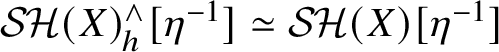 $\mathcal {SH}(X)_h^\wedge [\eta ^{-1}] \simeq \mathcal {SH}(X)[\eta ^{-1}]$
and similarly for
$\mathcal {SH}(X)_h^\wedge [\eta ^{-1}] \simeq \mathcal {SH}(X)[\eta ^{-1}]$
and similarly for
 $\rho $
. Thus, there is an equivalence
$\rho $
. Thus, there is an equivalence
 $$ \begin{align*} \mathcal{SH}(X)[\eta^{-1}]^{\text{cell}} \simeq \mathcal{SH}(x)[\eta^{-1}]^{\text{cell}}. \end{align*} $$
A similar equivalence holds for
 $\rho $
. With reference to Proposition 4, this shows (2) implies (3).
$\rho $
. With reference to Proposition 4, this shows (2) implies (3).
Example 3.4. We have
 $(E_{ab}^\wedge )_a^\wedge \simeq E_a^\wedge $
since
$(E_{ab}^\wedge )_a^\wedge \simeq E_a^\wedge $
since
 $ab$
-periodic objects are a-periodic. Hence, in Proposition 4, (2) implies (1).
$ab$
-periodic objects are a-periodic. Hence, in Proposition 4, (2) implies (1).
4 Topological models for stable motivic homotopy of regular number rings
We shall exhibit pullback squares describing
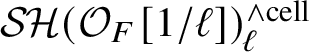 $\mathcal {SH}(\mathcal {O}_{F}[1/\ell ])_\ell ^{\wedge \text {cell}}$
for suitable number fields F and prime numbers
$\mathcal {SH}(\mathcal {O}_{F}[1/\ell ])_\ell ^{\wedge \text {cell}}$
for suitable number fields F and prime numbers
 $\ell $
in terms of
$\ell $
in terms of
 $\mathcal {SH}(k)_\ell ^{\wedge \text {cell}}$
for fields of the form
$\mathcal {SH}(k)_\ell ^{\wedge \text {cell}}$
for fields of the form
 $k=\mathbb C,\mathbb R,\mathbb {F}_{q}$
. To facilitate comparison with the work of Dwyer–Friedlander [Reference Röndigs, Spitzweck and Østvær24], we formally dualise our terminology and exhibit pushout squares in the opposite category.
$k=\mathbb C,\mathbb R,\mathbb {F}_{q}$
. To facilitate comparison with the work of Dwyer–Friedlander [Reference Röndigs, Spitzweck and Østvær24], we formally dualise our terminology and exhibit pushout squares in the opposite category.
4.1 Setup
Let
 $\ell $
be a prime (or, more generally, any integer, but we do not need or use this extra generality). We shall use the notation
$\ell $
be a prime (or, more generally, any integer, but we do not need or use this extra generality). We shall use the notation
 $\ell ' = \ell $
if
$\ell ' = \ell $
if
 $\ell $
is odd and
$\ell $
is odd and
 $\ell ' = \ell h$
if
$\ell ' = \ell h$
if
 $\ell =2$
.
$\ell =2$
.
Definition 5.
-
1. We write
for the full subcategory comprising functors
$$ \begin{align*} \mathcal{C\!M}_S \subset (\mathrm{CAlg}(\mathcal{P}\mathrm{r}^{\mathrm{L}})^{\mathrm{op}})_{/\mathcal{SH}(S)^{\text{cell}}} \end{align*} $$
$F\colon \mathcal {SH}(S)^{\text {cell}} \to \mathcal C$
, where
$\mathcal C$
is generated under colimits by
$F(\mathcal {SH}(S)^{\text {cell}})$
(or, equivalently, by
$F(S^{p,q})$
for
$p,q \in \mathbb {Z}$
).
-
2. We denote by
$M_{\ell '}$
the functor
$$ \begin{align*} \mathrm{S}\mathrm{ch}{}_{\mathbb{Z}[1/\ell]} \to \mathcal{C\!M}_{\mathbb{Z}[1/\ell]}, \quad X \mapsto \mathcal{SH}(X)_{\ell'}^{\wedge\text{cell}}, \quad (f: X \to Y) \mapsto (f^*: \mathcal{SH}(Y)_{\ell'}^{\wedge\text{cell}} \to \mathcal{SH}(X)_{\ell'}^{\wedge\text{cell}})^{\mathrm{op}}. \end{align*} $$


We also put
 $\mathcal {C\!M} = \mathcal {C\!M}_{\mathbb {Z}}$
and, by abuse of notation,
$\mathcal {C\!M} = \mathcal {C\!M}_{\mathbb {Z}}$
and, by abuse of notation,
 $M(X) := M_0(X) = \mathcal {SH}(X)^{\text {cell}} \in \mathcal {C\!M}$
. Note that
$M(X) := M_0(X) = \mathcal {SH}(X)^{\text {cell}} \in \mathcal {C\!M}$
. Note that
 $\mathcal {C\!M}_S = \mathcal {C\!M}_{/M_0(S)}$
and
$\mathcal {C\!M}_S = \mathcal {C\!M}_{/M_0(S)}$
and
 $M_{\ell '}(X) = M(X)_{\ell '}^\wedge $
. Next, we clarify the meaning of colimits in
$M_{\ell '}(X) = M(X)_{\ell '}^\wedge $
. Next, we clarify the meaning of colimits in
 $\mathcal {C\!M}_S$
.
$\mathcal {C\!M}_S$
.
Lemma 4.1. Let
 $F: I \to \mathcal {C\!M}_S$
be a diagram and write
$F: I \to \mathcal {C\!M}_S$
be a diagram and write
 $F': I^{\mathrm {op}} \to \mathcal {C}\mathrm {at}{}_\infty $
for the underlying diagram of categories. Then
$F': I^{\mathrm {op}} \to \mathcal {C}\mathrm {at}{}_\infty $
for the underlying diagram of categories. Then
 $\operatorname *{\mathrm {lim}}_{I^{\mathrm {op}}} F' \in \mathcal {C}\mathrm {at}{}_\infty $
is presentably symmetric monoidal and admits a natural functor from
$\operatorname *{\mathrm {lim}}_{I^{\mathrm {op}}} F' \in \mathcal {C}\mathrm {at}{}_\infty $
is presentably symmetric monoidal and admits a natural functor from
 $\mathcal {SH}(S)^{\text {cell}}$
. Let
$\mathcal {SH}(S)^{\text {cell}}$
. Let
 $\mathcal C$
denote its subcategory generated under colimits by the image of
$\mathcal C$
denote its subcategory generated under colimits by the image of
 $\mathcal {SH}(S)^{\text {cell}}$
. Then there is an equivalence
$\mathcal {SH}(S)^{\text {cell}}$
. Then there is an equivalence
 $\operatorname *{\mathrm {colim}}_I F \simeq \mathcal C$
.
$\operatorname *{\mathrm {colim}}_I F \simeq \mathcal C$
.
Proof. The forgetful functor
 $$ \begin{align*} \mathrm{CAlg}(\mathcal{P}\mathrm{r}^{\mathrm{L}})_{\mathcal{SH}(S)^{\text{cell}}/} \to \mathcal{C}\mathrm{at}{}_\infty \end{align*} $$
preserves limits [Reference Scheiderer48, Propositions 5.5.3.13, 1.2.13.8], [Reference Andradas, Bröcker and Ruiz49, Corollary 3.2.2.5], and hence the limit admits a canonical functor from
 $\mathcal {SH}(S)^{\text {cell}}$
. For
$\mathcal {SH}(S)^{\text {cell}}$
. For
 $\mathcal D \in \mathcal {C\!M}$
we have
$\mathcal D \in \mathcal {C\!M}$
we have
 $$ \begin{gather*} \mathrm{Map}_{\mathcal{C\!M}}(\mathcal C, \mathcal D) \simeq \mathrm{Map}_{\mathrm{CAlg}(\mathcal{P}\mathrm{r}^{\mathrm{L}})_{\mathcal{SH}(S)^{\text{cell}}/}}(\mathcal D, \mathcal C) \subset \mathrm{Map}_{\mathrm{CAlg}(\mathcal{P}\mathrm{r}^{\mathrm{L}})_{\mathcal{SH}(S)^{\text{cell}}/}}(\mathcal D, \operatorname*{\mathrm{lim}}_{I^{\mathrm{op}}} F') \\ \simeq \operatorname*{\mathrm{lim}}_{I^{\mathrm{op}}} \mathrm{Map}_{\mathrm{CAlg}(\mathcal{P}\mathrm{r}^{\mathrm{L}})_{\mathcal{SH}(S)^{\text{cell}}/}}(F(\mathord-), \mathcal D) \simeq \operatorname*{\mathrm{lim}}_{I^{\mathrm{op}}} \mathrm{Map}_{\mathcal{C\!M}}(F(\mathord-), \mathcal D). \end{gather*} $$
It remains to show the inclusion is an equivalence; that is, every map
 $\mathcal D \to \operatorname *{\mathrm {lim}}_{I^{\mathrm {op}}} F'$
in
$\mathcal D \to \operatorname *{\mathrm {lim}}_{I^{\mathrm {op}}} F'$
in
 $\mathrm {CAlg}(\mathcal {P}\mathrm {r}^{\mathrm {L}})_{\mathcal {SH}(S)^{\text {cell}}/}$
factors through
$\mathrm {CAlg}(\mathcal {P}\mathrm {r}^{\mathrm {L}})_{\mathcal {SH}(S)^{\text {cell}}/}$
factors through
 $\mathcal C$
. This holds for the generators, by assumption, so we are done.
$\mathcal C$
. This holds for the generators, by assumption, so we are done.
Next we reformulate and slightly extend our rigidity results from Section 3.
Lemma 4.2. Let
 $\bar {x}$
be the spectrum of a separably closed field,
$\bar {x}$
be the spectrum of a separably closed field,
 $X \in \mathrm {S}\mathrm {ch}{}_{\mathbb {Z}[1/\ell ]}$
an essentially smooth over a Dedekind domain,
$X \in \mathrm {S}\mathrm {ch}{}_{\mathbb {Z}[1/\ell ]}$
an essentially smooth over a Dedekind domain,
 $\bar x \to X$
a map and
$\bar x \to X$
a map and
 $y \in X$
a specialisation of the image of x. In
$y \in X$
a specialisation of the image of x. In
 $\mathcal {C\!M}_{\mathbb {Z}[1/\ell ]}$
there is a commutative diagram
$\mathcal {C\!M}_{\mathbb {Z}[1/\ell ]}$
there is a commutative diagram

Here the unlabelled maps are the canonical ones. In fact, there is a family of such commutative diagrams, parametrised by the (nonempty) set
 $X_y^h \times _X \bar x$
.
$X_y^h \times _X \bar x$
.
Proof. Let
 $X'$
be the henselisation of X along y. By [Reference Bachmann and Wickelgren71, Tags 03HV, 07QM(1)], the map
$X'$
be the henselisation of X along y. By [Reference Bachmann and Wickelgren71, Tags 03HV, 07QM(1)], the map
 $X' \to X$
hits the image of
$X' \to X$
hits the image of
 $\bar x$
, and hence there exists a lift
$\bar x$
, and hence there exists a lift
 $s'$
in the commutative diagram
$s'$
in the commutative diagram

Applying M and using that
 $M(y) \to M(X')$
is an equivalence by Proposition 4, the result follows.
$M(y) \to M(X')$
is an equivalence by Proposition 4, the result follows.
Corollary 6. The following hold under the assumptions in Lemma 4.2.
-
1. If
$y\in X$
is separably closed, then s is an equivalence. -
2. If
$\bar x, \bar y \in \mathrm {S}\mathrm {ch}{}_{\mathbb {Z}[1/\ell ]}$
are separably closed fields there is a (nonunique) equivalence
$M(\bar x) \simeq M(\bar y)$
.

Proof. (1) We have constructed a symmetric monoidal cocontinuous functor
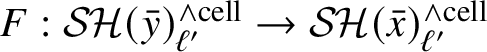 $F: \mathcal {SH}(\bar y)_{\ell '}^{\wedge \text {cell}} \to \mathcal {SH}(\bar x)_{\ell '}^{\wedge \text {cell}}$
under
$F: \mathcal {SH}(\bar y)_{\ell '}^{\wedge \text {cell}} \to \mathcal {SH}(\bar x)_{\ell '}^{\wedge \text {cell}}$
under
 $\mathcal {SH}(\mathbb {Z}[1/\ell ])^{\text {cell}}$
. Denote its right adjoint by G. Arguing as in the proof of Proposition 4, it suffices to show
$\mathcal {SH}(\mathbb {Z}[1/\ell ])^{\text {cell}}$
. Denote its right adjoint by G. Arguing as in the proof of Proposition 4, it suffices to show
 $\mathcal {E} \to GF \mathcal {E}$
is an equivalence. That is,
$\mathcal {E} \to GF \mathcal {E}$
is an equivalence. That is,
 $\mathcal {E} \to GF \mathcal {E}$
induces an isomorphism on
$\mathcal {E} \to GF \mathcal {E}$
induces an isomorphism on
 $\pi _{**}$
for
$\pi _{**}$
for
 $\mathcal {E} = \mathrm {H}\mathbb {F}_\ell $
,
$\mathcal {E} = \mathrm {H}\mathbb {F}_\ell $
,
 $\mathcal {E} = \mathrm {H}_{r\acute {e}t} \mathbb {Z}$
and, if
$\mathcal {E} = \mathrm {H}_{r\acute {e}t} \mathbb {Z}$
and, if
 $\ell $
is even,
$\ell $
is even,
 $\mathcal {E} = \mathbf {1}[\eta ^{-1}]$
. For any separably closed field of characteristic
$\mathcal {E} = \mathbf {1}[\eta ^{-1}]$
. For any separably closed field of characteristic
 $\ne \ell $
we have
$\ne \ell $
we have
 $\pi _{**}(\mathrm {H}\mathbb {F}_\ell ) \simeq \mathbb {F}_\ell [\tau ]$
(see, for example, [Reference Hoyois12, Corollary C.2(2)], [Reference Hornbostel and Yagunov40, Theorem 18.2.7]),
$\pi _{**}(\mathrm {H}\mathbb {F}_\ell ) \simeq \mathbb {F}_\ell [\tau ]$
(see, for example, [Reference Hoyois12, Corollary C.2(2)], [Reference Hornbostel and Yagunov40, Theorem 18.2.7]),
 $W = \mathbb {Z}/2$
and
$W = \mathbb {Z}/2$
and
 $\mathrm {H}_{r\acute {e}t} \mathbb {Z} = 0$
(the real spectrum being empty). Moreover, all of the maps are algebra maps over the corresponding algebra for
$\mathrm {H}_{r\acute {e}t} \mathbb {Z} = 0$
(the real spectrum being empty). Moreover, all of the maps are algebra maps over the corresponding algebra for
 $\mathbb {Z}[1/\ell ]$
. Thus, the map for
$\mathbb {Z}[1/\ell ]$
. Thus, the map for
 $\pi _{**} \mathrm {H}_{r\acute {e}t} \mathbb {Z}$
is trivially an isomorphism, and the one for
$\pi _{**} \mathrm {H}_{r\acute {e}t} \mathbb {Z}$
is trivially an isomorphism, and the one for
 $\pi _{**} \mathbf {1}[\eta ^{-1}]$
is an isomorphism because as an algebra it is determined by W according to [Reference Elmanto and Shah6, Proposition 5.2]. The isomorphism for
$\pi _{**} \mathbf {1}[\eta ^{-1}]$
is an isomorphism because as an algebra it is determined by W according to [Reference Elmanto and Shah6, Proposition 5.2]. The isomorphism for
 $\mathrm {H}\mathbb {F}_\ell $
will hold if and only if
$\mathrm {H}\mathbb {F}_\ell $
will hold if and only if
 $F(\tau ) = \tau $
, which holds provided
$F(\tau ) = \tau $
, which holds provided
 $F(\tau ^n) = \tau ^n$
for some
$F(\tau ^n) = \tau ^n$
for some
 $n \ge 1$
. But, for
$n \ge 1$
. But, for
 $n\gg 0$
,
$n\gg 0$
,
 $\tau ^n$
exists over
$\tau ^n$
exists over
 $\mathbb {Z}[1/\ell ]$
(if
$\mathbb {Z}[1/\ell ]$
(if
 $\ell =2$
, this holds with
$\ell =2$
, this holds with
 $n=1$
and for
$n=1$
and for
 $\ell $
odd; see, e.g., [Reference Washington9, §4.5(2)]).
$\ell $
odd; see, e.g., [Reference Washington9, §4.5(2)]).
(2) Let
 $x, y \in \mathrm {Spec}(\mathbb {Z}[1/\ell ])$
be the images of
$x, y \in \mathrm {Spec}(\mathbb {Z}[1/\ell ])$
be the images of
 $\bar x, \bar y$
. We may assume y is a specialisation of x. Let X be the strict henselisation of
$\bar x, \bar y$
. We may assume y is a specialisation of x. Let X be the strict henselisation of
 $\mathrm {Spec}(\mathbb {Z}[1/\ell ])$
along y, with closed point
$\mathrm {Spec}(\mathbb {Z}[1/\ell ])$
along y, with closed point
 $y'$
. By (1) applied with
$y'$
. By (1) applied with
 $X=X'$
we have
$X=X'$
we have
 $M(y') \simeq M(\bar x)$
, and by applying it with
$M(y') \simeq M(\bar x)$
, and by applying it with
 $(X, \bar x, y) = (\{y'\}, \bar y, y')$
we get
$(X, \bar x, y) = (\{y'\}, \bar y, y')$
we get
 $M(y') \simeq M(\bar y)$
.
$M(y') \simeq M(\bar y)$
.
Remark 4.3. This common category
 $M(\bar x) \simeq M(\bar y)$
is known as
$M(\bar x) \simeq M(\bar y)$
is known as
 $\ell $
-complete
$\ell $
-complete
 $\mathrm {MU}$
-based (even) synthetic spectra [Reference Gras59].
$\mathrm {MU}$
-based (even) synthetic spectra [Reference Gras59].
4.2 Criterion
Recall that for
 $X \in \mathrm {S}\mathrm {ch}{}_{\mathbb {Z}[1/\ell ]}$
the objects
$X \in \mathrm {S}\mathrm {ch}{}_{\mathbb {Z}[1/\ell ]}$
the objects
 $\mathrm {H}\mathbb {F}_\ell , \mathrm {H}_{r\acute {e}t} \mathbb {Z} \in \mathcal {SH}(X)$
are cellular and stable under base change. For
$\mathrm {H}\mathbb {F}_\ell , \mathrm {H}_{r\acute {e}t} \mathbb {Z} \in \mathcal {SH}(X)$
are cellular and stable under base change. For
 $\mathrm {H}\mathbb {F}_\ell $
this is [Reference Röndigs, Spitzweck and Østvær69, Corollary 10.4, Theorem 8.22]. For
$\mathrm {H}\mathbb {F}_\ell $
this is [Reference Röndigs, Spitzweck and Østvær69, Corollary 10.4, Theorem 8.22]. For
 $\mathrm {H}_{r\acute {e}t} \mathbb {Z}$
this follows from the expression
$\mathrm {H}_{r\acute {e}t} \mathbb {Z}$
this follows from the expression
 $\mathrm {H}_{r\acute {e}t} \mathbb {Z} \simeq o(\mathrm {H}\mathbb {Z})[1/\rho ]$
[Reference Behrens and Shah5], where
$\mathrm {H}_{r\acute {e}t} \mathbb {Z} \simeq o(\mathrm {H}\mathbb {Z})[1/\rho ]$
[Reference Behrens and Shah5], where
 $o: \mathcal {SH} \to \mathcal {SH}(X)$
is the unique cocontinuous symmetric monoidal functor. In particular, any morphism between
$o: \mathcal {SH} \to \mathcal {SH}(X)$
is the unique cocontinuous symmetric monoidal functor. In particular, any morphism between
 $M(X)$
and
$M(X)$
and
 $M(Y)$
in
$M(Y)$
in
 $\mathcal {C\!M}_{\mathbb {Z}[1/\ell ]}$
preserves these objects.
$\mathcal {C\!M}_{\mathbb {Z}[1/\ell ]}$
preserves these objects.
Proposition 7. Let
 $X_0, X_1, X_2, X_3 \in \mathrm {S}\mathrm {ch}{}_{\mathbb {Z}[1/\ell ]}$
be essentially smooth over Dedekind schemes and consider a commutative square
$X_0, X_1, X_2, X_3 \in \mathrm {S}\mathrm {ch}{}_{\mathbb {Z}[1/\ell ]}$
be essentially smooth over Dedekind schemes and consider a commutative square

in
 $\mathcal {C\!M}_{\mathbb {Z}[1/\ell ]}$
. In order for (4.1) to be co-Cartesian, it suffices that the following conditions hold:
$\mathcal {C\!M}_{\mathbb {Z}[1/\ell ]}$
. In order for (4.1) to be co-Cartesian, it suffices that the following conditions hold:
-
1. For each m, the square
is Cartesian. -
2. The square
is Cartesian. Here
$\mathbb {F}_\ell '$
equals
$\mathbb {F}_\ell $
if
$\ell =\ell '$
and
$\mathbb {Z}$
if
$\ell ' = \ell h$
(i.e., when
$\ell $
even).
-
3. If
$2 \mid \ell $
, then
$\mathrm {vcd}_2(K(X_i)) < \infty $
.


If
 $X_0$
contains a primitive
$X_0$
contains a primitive
 $\ell $
th root of unity, then condition (1) can be replaced by
$\ell $
th root of unity, then condition (1) can be replaced by
-
(1’) For each m, the square
is Cartesian.

Proof. To conclude that the square is co-Cartesian, it suffices, by Lemma 4.1, to prove the functor
 $$ \begin{align*} \mathcal{SH}(X_0)_{\ell'}^{\wedge\text{cell}} \to \mathcal{SH}(X_1)_{\ell'}^{\wedge\text{cell}} \times_{\mathcal{SH}(X_3)_{\ell'}^{\wedge\text{cell}}} \mathcal{SH}(X_2)_{\ell'}^{\wedge\text{cell}} \end{align*} $$
is fully faithful. Let us denote by
 $p_{1*}: \mathcal {SH}(X_1)_{\ell '}^{\wedge \text {cell}} \to \mathcal {SH}(X_0)_{\ell '}^{\wedge \text {cell}}$
the right adjoint of the functor corresponding to
$p_{1*}: \mathcal {SH}(X_1)_{\ell '}^{\wedge \text {cell}} \to \mathcal {SH}(X_0)_{\ell '}^{\wedge \text {cell}}$
the right adjoint of the functor corresponding to
 $M(X_1) \to M(X_0)$
, and similarly for
$M(X_1) \to M(X_0)$
, and similarly for
 $p_{2*}, p_{3*}$
. We need to prove that
$p_{2*}, p_{3*}$
. We need to prove that
 $$ \begin{align*} \pi_{**}(\mathbf{1}_{\ell'}^\wedge) \simeq \pi_{**}(p_{1*}(\mathbf{1}_{\ell'}^\wedge) \times_{p_{3*}\mathbf{1}_{\ell'}^\wedge}p_{2*}(\mathbf{1}_{\ell'}^\wedge)). \end{align*} $$
Note that each of the left adjoints preserves the compact generators, which is true for any morphism in
 $\mathcal {C\!M}$
, and hence
$\mathcal {C\!M}$
, and hence
 $p_{i*}$
preserves colimits and therefore it commutes with periodisation. Moreover,
$p_{i*}$
preserves colimits and therefore it commutes with periodisation. Moreover,
 $p_{i*}$
commutes with
$p_{i*}$
commutes with
 $\wedge \mathcal {E}$
for every
$\wedge \mathcal {E}$
for every
 $\mathcal {E} \in \mathcal {SH}(X_0)^{\wedge \text {cell}}_{\ell '}$
, and with completion at homotopy elements, by Lemma 3.1. We may check the desired equivalence after completing at
$\mathcal {E} \in \mathcal {SH}(X_0)^{\wedge \text {cell}}_{\ell '}$
, and with completion at homotopy elements, by Lemma 3.1. We may check the desired equivalence after completing at
 $\eta $
and after inverting
$\eta $
and after inverting
 $\eta $
, and similarly for other homotopy elements. For the
$\eta $
, and similarly for other homotopy elements. For the
 $\eta $
-periodic statement, we further invert
$\eta $
-periodic statement, we further invert
 $2$
respectively complete at
$2$
respectively complete at
 $2$
. In the
$2$
. In the
 $2$
-complete (still
$2$
-complete (still
 $\eta $
-periodic) case, either we have
$\eta $
-periodic) case, either we have
 $2 \nmid \ell $
and the statement is vacuous or
$2 \nmid \ell $
and the statement is vacuous or
 $1/2 \in X_i$
and using the fundamental fibre sequence [Reference Elmanto and Shah6, Corollary 1.2, Proposition 5.7], it suffices to establish the analogous equivalence for
$1/2 \in X_i$
and using the fundamental fibre sequence [Reference Elmanto and Shah6, Corollary 1.2, Proposition 5.7], it suffices to establish the analogous equivalence for
 $\mathrm {kw}_{2,\ell '}^\wedge $
. Recall that
$\mathrm {kw}_{2,\ell '}^\wedge $
. Recall that
 $\mathrm {kw}_{2,\ell '}^\wedge $
is in fact cellular [Reference Elmanto and Shah6, Proposition 5.7]. In the
$\mathrm {kw}_{2,\ell '}^\wedge $
is in fact cellular [Reference Elmanto and Shah6, Proposition 5.7]. In the
 $2$
-periodic (still
$2$
-periodic (still
 $\eta $
-periodic) case, arguing as in the proof of Proposition 4, it suffices to establish the analogous equivalence for
$\eta $
-periodic) case, arguing as in the proof of Proposition 4, it suffices to establish the analogous equivalence for
 $\mathrm {H}_{r\acute {e}t} \mathbb {F}_\ell '$
. For the
$\mathrm {H}_{r\acute {e}t} \mathbb {F}_\ell '$
. For the
 $\eta $
-complete statement, arguing as in the proof of Proposition 4, we have
$\eta $
-complete statement, arguing as in the proof of Proposition 4, we have
 $\mathbf {1}_{\eta ,\ell '}^\wedge \simeq \mathbf {1}_{\mathrm {H}\mathbb {F}_\ell }^\wedge $
and we see that it suffices to establish the analogous equivalence for
$\mathbf {1}_{\eta ,\ell '}^\wedge \simeq \mathbf {1}_{\mathrm {H}\mathbb {F}_\ell }^\wedge $
and we see that it suffices to establish the analogous equivalence for
 $\mathrm {H}\mathbb {F}_\ell $
. In summary, we need to prove the commutative square of ordinary spectra
$\mathrm {H}\mathbb {F}_\ell $
. In summary, we need to prove the commutative square of ordinary spectra

is Cartesian for all
 $* \in \mathbb {Z}$
and
$* \in \mathbb {Z}$
and
 $\mathcal {E}$
one of
$\mathcal {E}$
one of
 $\mathrm {kw}_{2,\ell '}^\wedge , \mathrm {H}\mathbb {F}_\ell , \mathrm {H}_{r\acute {e}t}\mathbb {F}_\ell '$
.
$\mathrm {kw}_{2,\ell '}^\wedge , \mathrm {H}\mathbb {F}_\ell , \mathrm {H}_{r\acute {e}t}\mathbb {F}_\ell '$
.
Before we start proving this, we need to make another preliminary remark. Suppose that

is a commutative diagram of filtered spectra such that
 ${\mathcal {E}}^{(i)}_n = 0$
for n sufficiently small and the induced diagrams of associated graded objects
${\mathcal {E}}^{(i)}_n = 0$
for n sufficiently small and the induced diagrams of associated graded objects

are pullbacks for each i. Then the square

is a pullback; indeed, an induction argument implies

is a pullback for every i.
Next we show how the conditions (1)–(3) imply that the squares are Cartesian. The pullback square for
 $\mathrm {H}_{r\acute {e}t} \mathbb {F}_\ell '$
is precisely condition (2), and the one for
$\mathrm {H}_{r\acute {e}t} \mathbb {F}_\ell '$
is precisely condition (2), and the one for
 $\mathrm {H}\mathbb {F}_\ell $
is precisely condition (1). The condition involving
$\mathrm {H}\mathbb {F}_\ell $
is precisely condition (1). The condition involving
 $\mathrm {kw}_{2,\ell '}^\wedge $
is only nonvacuous if
$\mathrm {kw}_{2,\ell '}^\wedge $
is only nonvacuous if
 $2 \mid \ell $
, whence
$2 \mid \ell $
, whence
 $1/2 \in X_i$
and
$1/2 \in X_i$
and
 $\mathrm {kw}_2^\wedge \simeq \mathrm {kw}_{2,\ell '}^\wedge $
. Consider the filtration of
$\mathrm {kw}_2^\wedge \simeq \mathrm {kw}_{2,\ell '}^\wedge $
. Consider the filtration of
 $\mathrm {kw}$
by powers of
$\mathrm {kw}$
by powers of
 $\beta $
, pulled back to
$\beta $
, pulled back to
 $X_i$
. The Postnikov filtration gives rise to the said filtration, and so it is complete, and
$X_i$
. The Postnikov filtration gives rise to the said filtration, and so it is complete, and
 $\mathrm {H}W$
gives all subquotients [Reference Elmanto and Shah6, Theorem 4.4, Lemma 4.3]. Since
$\mathrm {H}W$
gives all subquotients [Reference Elmanto and Shah6, Theorem 4.4, Lemma 4.3]. Since
 $\mathrm {kw}$
is connective, the preliminary remark allows us to replace
$\mathrm {kw}$
is connective, the preliminary remark allows us to replace
 $\mathrm {kw}_2^\wedge $
by
$\mathrm {kw}_2^\wedge $
by
 $\mathrm {H}W_2^\wedge $
, which on mapping spectra yields
$\mathrm {H}W_2^\wedge $
, which on mapping spectra yields
 $\Gamma (\mathord -, \underline {W}_2^\wedge )$
, where
$\Gamma (\mathord -, \underline {W}_2^\wedge )$
, where
 $\Gamma $
denotes global sections of a Nisnevich sheaf of spectra. On mapping spectra the cellular motivic spectrum
$\Gamma $
denotes global sections of a Nisnevich sheaf of spectra. On mapping spectra the cellular motivic spectrum
 $\underline {K}^W$
[Reference Elmanto and Shah6, Proposition 5.7, Theorem 4.4] yields compatible filtrations of
$\underline {K}^W$
[Reference Elmanto and Shah6, Proposition 5.7, Theorem 4.4] yields compatible filtrations of
 $\Gamma (\mathord -, \underline {W})$
by
$\Gamma (\mathord -, \underline {W})$
by
 $\Gamma (\mathord -, \underline {I}^n)$
(see [Reference Elmanto and Shah6, Definition 2.6]), where I is the fundamental ideal of even dimensional quadratic forms. Condition (3) together with [Reference Elmanto and Shah6, Proposition 2.3] implies
$\Gamma (\mathord -, \underline {I}^n)$
(see [Reference Elmanto and Shah6, Definition 2.6]), where I is the fundamental ideal of even dimensional quadratic forms. Condition (3) together with [Reference Elmanto and Shah6, Proposition 2.3] implies
 $\operatorname *{\mathrm {lim}}_n \Gamma (\mathord -, \underline {I}^n/2) \simeq 0$
. Thus, the filtration
$\operatorname *{\mathrm {lim}}_n \Gamma (\mathord -, \underline {I}^n/2) \simeq 0$
. Thus, the filtration
 $\Gamma (\mathord -, (\underline {W}/\underline {I}^n)_2^\wedge )$
of
$\Gamma (\mathord -, (\underline {W}/\underline {I}^n)_2^\wedge )$
of
 $\Gamma (\mathord -, \underline {W}_2^\wedge )$
is exhaustive. Using the preliminary remark, we may replace
$\Gamma (\mathord -, \underline {W}_2^\wedge )$
is exhaustive. Using the preliminary remark, we may replace
 $\Gamma (\mathord -, \underline {W}_2^\wedge )$
by
$\Gamma (\mathord -, \underline {W}_2^\wedge )$
by
 $\Gamma (\mathord -, \underline {I}^*/\underline {I}^{*+1})$
, which coincides with
$\Gamma (\mathord -, \underline {I}^*/\underline {I}^{*+1})$
, which coincides with
 $\mathrm {map}({\mathbb {G}_m^{\wedge *}}, (\mathrm {H}\mathbb {Z}/2)/\tau )$
according to [Reference Elmanto and Shah6, Theorem 2.1, Lemma 2.7]. For this, we may establish the pullback square for
$\mathrm {map}({\mathbb {G}_m^{\wedge *}}, (\mathrm {H}\mathbb {Z}/2)/\tau )$
according to [Reference Elmanto and Shah6, Theorem 2.1, Lemma 2.7]. For this, we may establish the pullback square for
 $\mathrm {H}\mathbb {F}_\ell $
, which implies the pullback square for
$\mathrm {H}\mathbb {F}_\ell $
, which implies the pullback square for
 $\mathrm {H}\mathbb {Z}_\ell ^\wedge $
and hence for
$\mathrm {H}\mathbb {Z}_\ell ^\wedge $
and hence for
 $\mathrm {H}\mathbb {Z}_\ell ^\wedge /2 \simeq \mathrm {H}\mathbb {Z}/2$
since
$\mathrm {H}\mathbb {Z}_\ell ^\wedge /2 \simeq \mathrm {H}\mathbb {Z}/2$
since
 $2 \mid \ell $
.
$2 \mid \ell $
.
Finally, suppose that
 $\zeta _\ell \in X_0$
. This yields
$\zeta _\ell \in X_0$
. This yields
 $\tau \in \pi _{0,-1}(\mathrm {H}\mathbb {F}_\ell )(X_0)$
given by the Bockstein on
$\tau \in \pi _{0,-1}(\mathrm {H}\mathbb {F}_\ell )(X_0)$
given by the Bockstein on
 $[\zeta _\ell ]$
. The cofibres of
$[\zeta _\ell ]$
. The cofibres of
 $\tau $
-powers yield a filtration of
$\tau $
-powers yield a filtration of
 $\mathrm {H}\mathbb {F}_\ell $
which pulls back to compatible filtrations on the
$\mathrm {H}\mathbb {F}_\ell $
which pulls back to compatible filtrations on the
 $X_i$
s. The explicit construction of the motivic complexes [Reference Röndigs, Spitzweck and Østvær69, Theorem 3.9] shows that these filtrations are bounded, separated and exhaustive and have subquotients
$X_i$
s. The explicit construction of the motivic complexes [Reference Röndigs, Spitzweck and Østvær69, Theorem 3.9] shows that these filtrations are bounded, separated and exhaustive and have subquotients
 $\Gamma _{\mathrm {Zar}}(X_i, R^m\epsilon _* \mathbb {F}_\ell )$
. Via the preliminary remark, the desired Cartesian square thus reduces to condition (1’).
$\Gamma _{\mathrm {Zar}}(X_i, R^m\epsilon _* \mathbb {F}_\ell )$
. Via the preliminary remark, the desired Cartesian square thus reduces to condition (1’).
Remark 4.4.
-
○ In all of our examples, the chain complexes in conditions (1’) and (2) will be concentrated in a single degree.
-
○ If
$\bar x$
is the spectrum of a separably closed field, then
$\Gamma _{\mathrm {Zar}}(\bar x, R^m\epsilon _* \mathbb {F}_\ell ) = 0$
for
$m> 0$
, and similarly
$\Gamma _{r\acute {e}t}(\bar x, \mathbb {Z}) = 0$
. -
○ If the square (4.1) in Proposition 7 is co-Cartesian, then conditions (1) and (2) hold and (1’) holds whenever
$\zeta _\ell \in X_0$
. Condition (3) is not necessary in general for the square to be co-Cartesian (consider, for example, any square comprising identity maps).


4.3 Models for stable motivic homotopy types
4.3.1 Arithmetic preliminaries
Lemma 4.5. Suppose K is a global field with ring of integers
 $\mathcal O_K$
and put
$\mathcal O_K$
and put
 $U = \mathrm {Spec}(\mathcal O_K[1/\ell ])$
. If
$U = \mathrm {Spec}(\mathcal O_K[1/\ell ])$
. If
 $\epsilon : U_{\acute {e}t} \to U_{\mathrm {Zar}}$
is the change of topology functor, then
$\epsilon : U_{\acute {e}t} \to U_{\mathrm {Zar}}$
is the change of topology functor, then
 $$ \begin{align*} R^i \epsilon_* \mu_\ell \simeq \begin{cases} \mu_\ell & i=0 \\ a_{\mathrm{Zar}} \mathcal O^\times/\ell & i=1 \\ a_{r\acute{e}t} \mathbb{Z}/(2,\ell) \oplus R & i=2 \\ a_{r\acute{e}t} \mathbb{Z}/(2,\ell) & i> 2 \end{cases}. \end{align*} $$
The sheaf R is determined by the exact sequence
 $$ \begin{align*} 0 \to R \to \bigoplus_{x \in \mathrm{Spec}(\mathcal O_K)^{(1)}} \mathbb{F}_\ell \to \mathbb{F}_\ell \oplus \bigoplus_{x \in U^{(1)}} i_{x*} \mathbb{F}_\ell \to 0. \end{align*} $$
Here the middle term is a constant sheaf, whereas the right-hand term is a sum of a constant sheaf and skyscraper sheaves, and the map is given by addition in the first component and restriction in the others.
Proof. From [Reference Bachmann, Kong, Wang and Xu52, Remark II.2.2] we can read off the isomorphisms
 $$ \begin{align*} R^0 \epsilon_* {\mathbb{G}_m} \simeq {\mathbb{G}_m}, \quad R^i \epsilon_* {\mathbb{G}_m} \simeq 0 \text{ for }i\text{ odd}, \quad R^i \epsilon_* {\mathbb{G}_m} \simeq a_{r\acute{e}t} \mathbb R^\times \text{ for }i \ge 4\text{ even} \end{align*} $$
and the short exact sequence
 $$ \begin{align*} 0 \to R^2 \epsilon_* {\mathbb{G}_m} \to a_{r\acute{e}t} \mathbb{Z}/2 \oplus \bigoplus_{x \in \mathrm{Spec}(\mathcal O_K)^{(1)}} \mathbb{Q}/\mathbb{Z} \to \mathbb{Q}/\mathbb{Z} \oplus \bigoplus_{x \in U^{(1)}} i_{x*} \mathbb{Q}/\mathbb{Z} \to 0. \end{align*} $$
For the exact sequence, recall
 $Br(K_v) = \mathbb {Z}/2$
if v is a real place,
$Br(K_v) = \mathbb {Z}/2$
if v is a real place,
 $=0$
if v is a complex place and
$=0$
if v is a complex place and
 $=\mathbb {Q}/\mathbb {Z}$
if v is a non-Archimedean place [Reference Röndigs, Spitzweck and Østvær67, p. 163, 193]. Moreover, the kernel of the restriction map is precisely the sum over the non-Archimedean places missing in U. The Kummer short exact sequence
$=\mathbb {Q}/\mathbb {Z}$
if v is a non-Archimedean place [Reference Röndigs, Spitzweck and Østvær67, p. 163, 193]. Moreover, the kernel of the restriction map is precisely the sum over the non-Archimedean places missing in U. The Kummer short exact sequence
 $$ \begin{align*} 0 \to \mu_\ell \to {\mathbb{G}_m} \xrightarrow{\ell} {\mathbb{G}_m} \to 0 \end{align*} $$
on
 $U_{\acute {e}t}$
yields a long exact sequence for
$U_{\acute {e}t}$
yields a long exact sequence for
 $R^i\epsilon _*$
. Since
$R^i\epsilon _*$
. Since
 $R^i\epsilon _* {\mathbb {G}_m}$
vanishes in odd degrees,
$R^i\epsilon _* {\mathbb {G}_m}$
vanishes in odd degrees,
 $R^i\epsilon _* \mu _\ell $
is given by the kernel or cokernel of multiplication by
$R^i\epsilon _* \mu _\ell $
is given by the kernel or cokernel of multiplication by
 $\ell $
. This immediately yields the desired results for
$\ell $
. This immediately yields the desired results for
 $i \ne 2,3$
, and the snake lemma produces an exact sequence
$i \ne 2,3$
, and the snake lemma produces an exact sequence
 $$ \begin{align*} 0 \to R^2 \epsilon_* \mu_\ell \to a_{r\acute{e}t} \mathbb{Z}/(2,\ell) \oplus \bigoplus_{x \in \mathrm{Spec}(\mathcal O_K)^{(1)}} \mathbb{F}_\ell \xrightarrow{b} \mathbb{F}_\ell \oplus \bigoplus_{x \in U^{(1)}} i_{x*} \mathbb{F}_\ell \to R^3 \epsilon_* \mu_\ell \to a_{r\acute{e}t} \mathbb{Z}/(2,\ell) \to 0. \end{align*} $$
Since b is a surjection of Zariski sheaves, the result follows.
Corollary 8. Suppose
 $Pic(U)$
is uniquely
$Pic(U)$
is uniquely
 $\ell $
-divisible and
$\ell $
-divisible and
 $k(U)$
has a unique place of characteristic
$k(U)$
has a unique place of characteristic
 $\ell $
. Then
$\ell $
. Then
 $H^j(U, R^i \epsilon _* \mu _\ell ) = 0$
for
$H^j(U, R^i \epsilon _* \mu _\ell ) = 0$
for
 $j>0$
and
$j>0$
and
 $$ \begin{align*} H^0(U, R^i\epsilon_* \mu_\ell) \simeq \begin{cases} \mu_\ell(U) & i=0 \\ \mathcal O^\times(U)/\ell & i=1 \\ (\mathbb{Z}/(2,\ell))^{\mathrm{Sper}(K)} & i>1. \end{cases} \end{align*} $$
Proof. Since
 $\mu _\ell |_{U_{\mathrm {Zar}}}$
is constant and constant sheaves are flasque, the claims for
$\mu _\ell |_{U_{\mathrm {Zar}}}$
is constant and constant sheaves are flasque, the claims for
 $i=0$
are clear. The claims about
$i=0$
are clear. The claims about
 $a_{r\acute {e}t} \mathbb {Z}/(2,\ell )$
follow because
$a_{r\acute {e}t} \mathbb {Z}/(2,\ell )$
follow because
 $R(U) \simeq \mathrm {Sper}(k)$
is discrete. Since the Zariski cohomological dimension of U is
$R(U) \simeq \mathrm {Sper}(k)$
is discrete. Since the Zariski cohomological dimension of U is
 $1$
, it remains to show that
$1$
, it remains to show that
 $H^0_{\mathrm {Zar}}(U, {\mathbb {G}_m}/\ell ) \simeq \mathcal O^\times (U)/\ell $
,
$H^0_{\mathrm {Zar}}(U, {\mathbb {G}_m}/\ell ) \simeq \mathcal O^\times (U)/\ell $
,
 $H^1_{\mathrm {Zar}}(U, {\mathbb {G}_m}/\ell ) = 0$
, and
$H^1_{\mathrm {Zar}}(U, {\mathbb {G}_m}/\ell ) = 0$
, and
 $H^*_{\mathrm {Zar}}(U, R) = 0$
for
$H^*_{\mathrm {Zar}}(U, R) = 0$
for
 $*=0, 1$
. Using the short exact sequences
$*=0, 1$
. Using the short exact sequences
 $0 \to \mu _\ell \to {\mathbb {G}_m} \to \ell {\mathbb {G}_m} \to 0$
and
$0 \to \mu _\ell \to {\mathbb {G}_m} \to \ell {\mathbb {G}_m} \to 0$
and
 $0 \to \ell {\mathbb {G}_m} \to {\mathbb {G}_m} \to {\mathbb {G}_m}/\ell \to 0$
, the first two claims are equivalent to unique
$0 \to \ell {\mathbb {G}_m} \to {\mathbb {G}_m} \to {\mathbb {G}_m}/\ell \to 0$
, the first two claims are equivalent to unique
 $\ell $
-divisibility of
$\ell $
-divisibility of
 $Pic(U)$
. The exact sequence defining R is, in fact, a flasque resolution, so its
$Pic(U)$
. The exact sequence defining R is, in fact, a flasque resolution, so its
 $H^0$
and
$H^0$
and
 $H^1$
are given by the kernel and cokernel of the induced map on global sections. This induced map is an isomorphism as needed if and only if
$H^1$
are given by the kernel and cokernel of the induced map on global sections. This induced map is an isomorphism as needed if and only if
 $\mathrm {Spec}(\mathcal O_K) \setminus U$
consists of precisely one point, which holds by assumption.
$\mathrm {Spec}(\mathcal O_K) \setminus U$
consists of precisely one point, which holds by assumption.
Lemma 4.6. Let
 $\ell $
be prime, K a global field and
$\ell $
be prime, K a global field and
 $U \subset Spec(\mathcal O_K)$
open. Let
$U \subset Spec(\mathcal O_K)$
open. Let
 $H \subset \mathcal O^\times (U)/\ell $
be an arbitrary subgroup. There exist
$H \subset \mathcal O^\times (U)/\ell $
be an arbitrary subgroup. There exist
 $x_1, \dots , x_n \in U^{(1)}$
such that the restriction
$x_1, \dots , x_n \in U^{(1)}$
such that the restriction
 $$ \begin{align*} H \subset \mathcal O^\times(U)/\ell \to \prod_i k(x)^\times/\ell \end{align*} $$
is an isomorphism. If H is nontrivial, there exist infinitely many such choices.
Proof. First recall the following fact (see, e.g., [Reference Serre56, Exercise VI.1.2]): If
 $a \in \mathcal O(U)$
is an
$a \in \mathcal O(U)$
is an
 $\ell $
th power in
$\ell $
th power in
 $k(x)$
for all but finitely many
$k(x)$
for all but finitely many
 $x \in U^{(1)}$
, then a is an
$x \in U^{(1)}$
, then a is an
 $\ell $
th power.
$\ell $
th power.
If H is nontrivial, pick
 $1 \ne a \in H$
. Since H is a
$1 \ne a \in H$
. Since H is a
 $\mathbb {Z}/\ell $
-vector space, we may write
$\mathbb {Z}/\ell $
-vector space, we may write
 $H = \langle a \rangle \times H'$
, where
$H = \langle a \rangle \times H'$
, where
 $\langle a \rangle \simeq \mathbb {Z}/\ell $
is the subgroup generated by a. By the above fact, there exists
$\langle a \rangle \simeq \mathbb {Z}/\ell $
is the subgroup generated by a. By the above fact, there exists
 $x \in U^{(1)}$
such that the image of a in
$x \in U^{(1)}$
such that the image of a in
 $k(x)^\times /\ell $
is nonzero and in fact infinitely many choices of x. Since
$k(x)^\times /\ell $
is nonzero and in fact infinitely many choices of x. Since
 $k(x)$
is finite,
$k(x)$
is finite,
 $k(x)^\times /\ell \simeq \mathbb {Z}/\ell \simeq \langle a \rangle $
. We are thus reduced to proving the result for
$k(x)^\times /\ell \simeq \mathbb {Z}/\ell \simeq \langle a \rangle $
. We are thus reduced to proving the result for
 $H'$
and conclude by induction since
$H'$
and conclude by induction since
 $\mathcal O^\times (U)/\ell $
is finite according to Dirichlet’s unit theorem [Reference Serre56, Corollary 11.7].
$\mathcal O^\times (U)/\ell $
is finite according to Dirichlet’s unit theorem [Reference Serre56, Corollary 11.7].
In [Reference Bachmann30], Gras introduced the narrow tame kernel
 $K_{2}^{+}(\mathcal O_{F})$
as the subgroup of
$K_{2}^{+}(\mathcal O_{F})$
as the subgroup of
 $K_{2}(\mathcal O_{F})$
where the regular symbols on all of the real embeddings of F vanish; that is, there is an exact sequence
$K_{2}(\mathcal O_{F})$
where the regular symbols on all of the real embeddings of F vanish; that is, there is an exact sequence
 $$ \begin{align*} 0\to K_{2}^{+}(\mathcal O_{F}) \to K_{2}(\mathcal O_{F}) \to \bigoplus^{r}\mathbb{Z}/2 \to 0. \end{align*} $$
We refer to [Reference Berrick, Karoubi and Østvær31, Definition 7.8.1] for the arithmetic notion of
 $\ell $
-regular number fields.
$\ell $
-regular number fields.
Definition 9. Let
 $\ell $
be a prime number. A number field F is called
$\ell $
be a prime number. A number field F is called
 $\ell $
-regular if the
$\ell $
-regular if the
 $\ell $
-Sylow subgroup of the narrow tame kernel
$\ell $
-Sylow subgroup of the narrow tame kernel
 $K_{2}^{+}(\mathcal O_{F})$
is trivial.
$K_{2}^{+}(\mathcal O_{F})$
is trivial.
See [Reference Bachmann30], [Reference Milnor and Husemoller32], [Reference Gras and Jaulent60], [Reference Bökstedt15] for complementary results about these families of number fields. For example, the field of rational numbers
 $\mathbb {Q}$
is
$\mathbb {Q}$
is
 $\ell $
-regular for every prime
$\ell $
-regular for every prime
 $\ell $
, and
$\ell $
, and
 $\mathbb {Q}(\zeta _\ell )$
is
$\mathbb {Q}(\zeta _\ell )$
is
 $\ell $
-regular if
$\ell $
-regular if
 $\ell $
is a regular prime number in the sense of Kummer [Reference Morel73]. In [Reference Kylling, Röndigs and Østvær68], Siegel conjectured there are infinitely many regular prime numbers.
$\ell $
is a regular prime number in the sense of Kummer [Reference Morel73]. In [Reference Kylling, Röndigs and Østvær68], Siegel conjectured there are infinitely many regular prime numbers.
We have the following explicit characterisation of
 $\ell $
-regular number fields.
$\ell $
-regular number fields.
Proposition 10. Let F be a number field. We write
 ${\mathcal O}_{F}^{\prime }$
for the ring of
${\mathcal O}_{F}^{\prime }$
for the ring of
 $\ell $
-integers
$\ell $
-integers
 $\mathcal O_F[1/\ell ]$
.
$\mathcal O_F[1/\ell ]$
.
-
1. F is
$2$
-regular if and only if the prime ideal
$(2)$
does not split in
$F/\mathbb {Q}$
and the narrow Picard group
$Pic_{+}({\mathcal O}_{F}^{\prime })$
has odd order. -
2. Let
$\ell $
be an odd prime number and assume
$\mu _{\ell }\subset F$
. Then F is
$\ell $
-regular if and only if the prime ideal
$(\ell )$
does not split in
$F/\mathbb {Q}$
and the
$\ell $
-Sylow subgroup of the Picard group
$Pic({\mathcal O}_{F}^{\prime })$
is trivial. -
3. Let
$\ell $
be an odd prime number. Assume
$\mu _{\ell }\not \subset F$
and F contains the maximal real subfield of
$\mathbb {Q}(\zeta _{\ell })$
. Then F is
$\ell $
-regular if and only if the prime ideals above
$(\ell )$
in F do not split in the quadratic extension
$F(\zeta _{\ell })/F$
and the
$\ell $
-Sylow subgroups of the Picard groups
$Pic({\mathcal O}_{F})$
and
$Pic({\mathcal O}_{F(\zeta _{\ell })})$
are isomorphic.


Proof. This is a reformulation of [Reference Bachmann30, Corollary on pp. 328-329]. See also [Reference Gras and Jaulent60, Proposition 2.2] when
 $\ell =2$
.
$\ell =2$
.
For further reference, we recall that a commutative square of abelian groups

is called bi-Cartesian if it is a pullback when viewed as a commutative square of spectra.
4.3.2 Stable motivic homotopy types of 2-regular number fields
Theorem 4.7. Suppose F is a
 $2$
-regular number field with r real and c pairs of complex embeddings. Let
$2$
-regular number field with r real and c pairs of complex embeddings. Let
 $x, y_1, \dots , y_{c} \in \mathrm {Spec}({\mathcal O}_{F}^{\prime })$
be closed points.
$x, y_1, \dots , y_{c} \in \mathrm {Spec}({\mathcal O}_{F}^{\prime })$
be closed points.
-
1. There is a canonical commutative square in
$\mathcal {C\!M}$
-
2. The square in (1) is a pushout if and only if there is a naturally induced isomorphism
$$ \begin{align*} ({\mathcal O}_{F}^{\prime})^\times/2 \simeq (\mathbb R^\times/2)^{r} \times k(x)^\times/2 \times \prod_i k(y_i)^\times/2 \quad (\simeq (\mathbb{Z}/2)^{1+r+c}). \end{align*} $$
-
3. There exist infinitely many choices of
$x, y_1, \dots , y_{c}$
such that the map in (2) is an isomorphism.


Proof. To simplify notation, throughout this proof we put
 $M := M_{2h}$
.
$M := M_{2h}$
.
(1) For
 $z \in \mathrm {Spec}({\mathcal O}_{F}^{\prime })$
and
$z \in \mathrm {Spec}({\mathcal O}_{F}^{\prime })$
and
 $\alpha : K \hookrightarrow \mathbb C$
, Lemma 4.2 furnishes a map
$\alpha : K \hookrightarrow \mathbb C$
, Lemma 4.2 furnishes a map
 $f_{z,\alpha }: M(\mathbb C) \to M(z)$
and a homotopy between
$f_{z,\alpha }: M(\mathbb C) \to M(z)$
and a homotopy between
 $M(\mathbb C) \to M(z) \to M({\mathcal O}_{F}^{\prime })$
, and the map
$M(\mathbb C) \to M(z) \to M({\mathcal O}_{F}^{\prime })$
, and the map
 $M(\mathbb C) \to M({\mathcal O}_{F}^{\prime })$
induced by
$M(\mathbb C) \to M({\mathcal O}_{F}^{\prime })$
induced by
 $\alpha $
. In (1), the bottom and right-hand maps are the canonical ones. Write
$\alpha $
. In (1), the bottom and right-hand maps are the canonical ones. Write
 $\alpha _1, \bar \alpha _1, \dots , \alpha _c, \bar \alpha _c, \beta _1, \dots , \beta _r$
for the complex and real embeddings. Let
$\alpha _1, \bar \alpha _1, \dots , \alpha _c, \bar \alpha _c, \beta _1, \dots , \beta _r$
for the complex and real embeddings. Let
 $\alpha _{c+i} = \iota \circ \beta _i$
, where
$\alpha _{c+i} = \iota \circ \beta _i$
, where
 $\iota : \mathbb R \to \mathbb C$
is the canonical embedding. The left-hand map is
$\iota : \mathbb R \to \mathbb C$
is the canonical embedding. The left-hand map is
 $f_{x,\alpha _i}$
on component i. The top map is
$f_{x,\alpha _i}$
on component i. The top map is
 $f_{y_i, \alpha _i}$
on the ith component if
$f_{y_i, \alpha _i}$
on the ith component if
 $i \le c$
and induced by
$i \le c$
and induced by
 $\iota $
on the remaining components. In all cases, the induced composite map
$\iota $
on the remaining components. In all cases, the induced composite map
 $M(\mathbb C) \to M({\mathcal O}_{F}^{\prime })$
is either equal or homotopic to the map induced by
$M(\mathbb C) \to M({\mathcal O}_{F}^{\prime })$
is either equal or homotopic to the map induced by
 $\alpha _i$
. Thus, the square commutes.
$\alpha _i$
. Thus, the square commutes.
(2) We use the criterion from Proposition 7. Condition (3) holds since the fields are finitely generated. For condition (2), the square

is clearly bi-Cartesian because the map
 ${\mathcal O}_{F}^{\prime } \to \mathbb R^r$
induces an isomorphism on real spectra.
${\mathcal O}_{F}^{\prime } \to \mathbb R^r$
induces an isomorphism on real spectra.
Next we check condition (1’). Owing to [Reference Bökstedt15, Proposition 2.1(5)] the
 $2$
-regularity assumption implies
$2$
-regularity assumption implies
 $Pic({\mathcal O}_{F}^{\prime })$
has odd order, so it is uniquely
$Pic({\mathcal O}_{F}^{\prime })$
has odd order, so it is uniquely
 $2$
-divisible, and F has only one place of characteristic
$2$
-divisible, and F has only one place of characteristic
 $2$
. Thus, Corollary 8 applies and it remains to check the bicartesianess of three squares. The first one is
$2$
. Thus, Corollary 8 applies and it remains to check the bicartesianess of three squares. The first one is

Observe that if
 $X, Y$
are connected schemes and
$X, Y$
are connected schemes and
 $f: M(X) \to M(Y)$
is any map in
$f: M(X) \to M(Y)$
is any map in
 $\mathcal {C\!M}_{\mathbb {Z}[1/2]}$
, then
$\mathcal {C\!M}_{\mathbb {Z}[1/2]}$
, then
 $f^*: H^0(Y, \mathbb {Z}/2) \to H^0(X, \mathbb {Z}/2)$
is an isomorphism. Indeed, this reduces to the case of the structure map
$f^*: H^0(Y, \mathbb {Z}/2) \to H^0(X, \mathbb {Z}/2)$
is an isomorphism. Indeed, this reduces to the case of the structure map
 $M(X) \to M(\mathbb {Z}[1/2])$
, where it is obvious. Thus, the square for
$M(X) \to M(\mathbb {Z}[1/2])$
, where it is obvious. Thus, the square for
 $m=0$
is bi-Cartesian because the vertical maps are isomorphisms. When
$m=0$
is bi-Cartesian because the vertical maps are isomorphisms. When
 $m=2$
, the square is the same as in condition (2) above and hence it is bi-Cartesian. The remaining square for
$m=2$
, the square is the same as in condition (2) above and hence it is bi-Cartesian. The remaining square for
 $m=1$
takes the form
$m=1$
takes the form

Since the inclusion of abelian groups into spectra preserves finite products, this square is bi-Cartesian if and only if the stated condition holds.
(3) Dirichlet’s unit theorem [Reference Serre56, Corollary 11.7] implies
 $({\mathcal O}_{F}^{\prime })^\times \simeq \mu ({\mathcal O}_{F}^{\prime }) \times \mathbb {Z}^{r+c}$
; here
$({\mathcal O}_{F}^{\prime })^\times \simeq \mu ({\mathcal O}_{F}^{\prime }) \times \mathbb {Z}^{r+c}$
; here
 $\mu ({\mathcal O}_{F}^{\prime })$
is the finite abelian group of roots of unity in
$\mu ({\mathcal O}_{F}^{\prime })$
is the finite abelian group of roots of unity in
 ${\mathcal O}_{F}^{\prime }$
. It is cyclic, being a finite multiplicative subgroup of a field, and since
${\mathcal O}_{F}^{\prime }$
. It is cyclic, being a finite multiplicative subgroup of a field, and since
 $\{\pm 1\} \in \mu ({\mathcal O}_{F}^{\prime })$
, the group has even order. It follows that
$\{\pm 1\} \in \mu ({\mathcal O}_{F}^{\prime })$
, the group has even order. It follows that
 $({\mathcal O}_{F}^{\prime })^\times /2 \simeq \mathbb {Z}/2 \times (\mathbb {Z}/2)^{r+c}$
. Moreover,
$({\mathcal O}_{F}^{\prime })^\times /2 \simeq \mathbb {Z}/2 \times (\mathbb {Z}/2)^{r+c}$
. Moreover,
 $2$
-regularity implies the naturally induced map
$2$
-regularity implies the naturally induced map
 $({\mathcal O}_{F}^{\prime })^\times /2 \to (\mathbb R^\times /2)^{r} \simeq (\mathbb {Z}/2)^{r}$
is surjective [Reference Bökstedt15, Proposition 2.1(5)]; we write
$({\mathcal O}_{F}^{\prime })^\times /2 \to (\mathbb R^\times /2)^{r} \simeq (\mathbb {Z}/2)^{r}$
is surjective [Reference Bökstedt15, Proposition 2.1(5)]; we write
 $U_+ \simeq (\mathbb {Z}/2)^{1+c}$
for its kernel. The condition in part (2) holds if and only if the induced map
$U_+ \simeq (\mathbb {Z}/2)^{1+c}$
for its kernel. The condition in part (2) holds if and only if the induced map
 $U_+ \to k(x)^\times /2 \times \prod _i k(y_i)^\times /2$
is an isomorphism. Lemma 4.6 implies the latter is true for infinitely many choices of
$U_+ \to k(x)^\times /2 \times \prod _i k(y_i)^\times /2$
is an isomorphism. Lemma 4.6 implies the latter is true for infinitely many choices of
 $x, y_i$
.
$x, y_i$
.
Remark 4.8. As in Examples 3.3 and 3.4, Theorem 4.7(1) implies similar pushout squares with respect to completions at
 $2$
, h and with respect to periodisations at
$2$
, h and with respect to periodisations at
 $\rho $
,
$\rho $
,
 $\eta $
. For example, we have a pushout square in
$\eta $
. For example, we have a pushout square in
 $\mathcal {C\!M}$

Remark 4.9. The various embeddings
 $\alpha _i: K \to \mathbb C$
differ by automorphisms of
$\alpha _i: K \to \mathbb C$
differ by automorphisms of
 $\mathbb C$
. It follows that one may choose the maps
$\mathbb C$
. It follows that one may choose the maps
 $f_{x,\alpha _i}$
to be of the form
$f_{x,\alpha _i}$
to be of the form
 $\sigma _i \circ f_{x,\alpha _1}$
. Thus, applying an automorphism of
$\sigma _i \circ f_{x,\alpha _1}$
. Thus, applying an automorphism of
 $M_{2h}(\mathbb C^{r+s})$
in the square of Theorem 4.7, we may assume that all of the left-hand vertical maps
$M_{2h}(\mathbb C^{r+s})$
in the square of Theorem 4.7, we may assume that all of the left-hand vertical maps
 $M_{2h}(\mathbb C) \to M_{2h}(x)$
are the same. The square being a pushout now is equivalent to saying that there are lifts of
$M_{2h}(\mathbb C) \to M_{2h}(x)$
are the same. The square being a pushout now is equivalent to saying that there are lifts of
 $M_{2h}(x), M_{2h}(y_i)$
to
$M_{2h}(x), M_{2h}(y_i)$
to
 $\mathcal {C\!M}_{M_{2h}(\mathbb C)/}$
and an equivalence
$\mathcal {C\!M}_{M_{2h}(\mathbb C)/}$
and an equivalence
 $$ \begin{align*} M_{2h}({\mathcal O}_{F}^{\prime}) \simeq \bigvee^r M_{2h}(\mathbb R) \vee M_{2h}(x) \vee \bigvee^c M_{2h}(y_i). \end{align*} $$
Here
 $\vee $
denotes the coproduct in
$\vee $
denotes the coproduct in
 $\mathcal {C\!M}_{M(\mathbb C)/}$
.
$\mathcal {C\!M}_{M(\mathbb C)/}$
.
Example 4.10. When
 $F=\mathbb {Q}$
, we consider
$F=\mathbb {Q}$
, we consider
 $\mathbb {Z}[1/2]^\times \simeq \{\pm 1\} \times \{(1/2)^n\}$
and
$\mathbb {Z}[1/2]^\times \simeq \{\pm 1\} \times \{(1/2)^n\}$
and
 $\mathbb {Z}[1/2]^\times /2 \simeq \mathbb {Z}/2\{-1, 2\}$
. Here
$\mathbb {Z}[1/2]^\times /2 \simeq \mathbb {Z}/2\{-1, 2\}$
. Here
 $\mathbb {Z}/2\{2\}$
is the kernel of the surjection
$\mathbb {Z}/2\{2\}$
is the kernel of the surjection
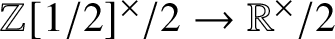 $\mathbb {Z}[1/2]^\times /2\to \mathbb R^\times /2$
. We need to find a closed point
$\mathbb {Z}[1/2]^\times /2\to \mathbb R^\times /2$
. We need to find a closed point
 $x \in \mathrm {Spec}(\mathbb {Z}[1/2])$
such that
$x \in \mathrm {Spec}(\mathbb {Z}[1/2])$
such that
 $2$
is not a square in
$2$
is not a square in
 $k(x)$
. This holds when
$k(x)$
. This holds when
 $k(x) = \mathrm {Spec}(\mathbb {F}_q)$
, where
$k(x) = \mathrm {Spec}(\mathbb {F}_q)$
, where
 $q\equiv \pm 3\bmod 8$
. In particular, the canonical map
$q\equiv \pm 3\bmod 8$
. In particular, the canonical map
 $$ \begin{align*} \mathcal{SH}(\mathbb{Z}[1/2])_2^{\wedge\text{cell}} \to \mathcal{SH}(\mathbb R)_2^{\wedge\text{cell}} \times_{\mathcal{SH}(\mathbb C)_2^{\wedge\text{cell}}} \mathcal{SH}(\mathbb{F}_3)_2^{\wedge\text{cell}} \end{align*} $$
is fully faithful. To deduce Theorem 1.2 from the introduction, let
 $\mathcal E \in \mathcal {SH}(\mathbb {Z}[1/2])_2^{\wedge \text {cell}}$
and compute
$\mathcal E \in \mathcal {SH}(\mathbb {Z}[1/2])_2^{\wedge \text {cell}}$
and compute
 $\mathrm {map}(\mathbf {1}, \mathcal E)$
using the above square.
$\mathrm {map}(\mathbf {1}, \mathcal E)$
using the above square.
4.3.3 Stable motivic homotopy types of
$\ell $
-regular number fields

Theorem 4.11. Let F be a number field with c pairs of complex embeddings and
 $\ell $
be an odd prime number. Suppose F is
$\ell $
be an odd prime number. Suppose F is
 $\ell $
-regular and
$\ell $
-regular and
 $\mu _{\ell }\subset F$
. Let
$\mu _{\ell }\subset F$
. Let
 $x, y_1, \dots , y_c \in \mathrm {Spec}({\mathcal O}_{F}^{\prime })$
be closed points.
$x, y_1, \dots , y_c \in \mathrm {Spec}({\mathcal O}_{F}^{\prime })$
be closed points.
-
1. There is a canonical commutative square in
$\mathcal {C\!M}$
-
2. The square is a pushout if and only if there is a naturally induced isomorphism
$$ \begin{align*} ({\mathcal O}_{F}^{\prime})^\times/\ell \simeq k(x)^\times/\ell \times \prod_{i} k(y_i)^\times/\ell \quad (\simeq (\mathbb{F}_\ell)^{1+c}). \end{align*} $$
-
3. There exist infinitely many choices of
$x,y_1, \dots , y_c$
satisfying (2).


Proof. The proof is essentially the same as that of Theorem 4.7. The maps
 $x, y_i\to \mathrm {Spec}({\mathcal O}_{F}^{\prime })$
together with choices of embeddings of K into
$x, y_i\to \mathrm {Spec}({\mathcal O}_{F}^{\prime })$
together with choices of embeddings of K into
 $\mathbb C$
induce, via Lemma 4.2, the maps
$\mathbb C$
induce, via Lemma 4.2, the maps
 $M_\ell (\mathbb C) \to M_\ell (x),M_\ell (y_i)$
in the commutative square. One verifies, using Corollary 8 and
$M_\ell (\mathbb C) \to M_\ell (x),M_\ell (y_i)$
in the commutative square. One verifies, using Corollary 8 and
 $\mathbb {Z}/(2, \ell ) = 0$
, that condition (1’) of Proposition 7 reduces to the condition stated in (2). The other conditions hold trivially; since K contains a primitive
$\mathbb {Z}/(2, \ell ) = 0$
, that condition (1’) of Proposition 7 reduces to the condition stated in (2). The other conditions hold trivially; since K contains a primitive
 $\ell $
th root of unity, the real spectrum
$\ell $
th root of unity, the real spectrum
 $\mathrm {Sper}({\mathcal O}_{F}^{\prime }) = \emptyset $
. The existence of infinitely many choices in (3) follows from Lemma 4.6.
$\mathrm {Sper}({\mathcal O}_{F}^{\prime }) = \emptyset $
. The existence of infinitely many choices in (3) follows from Lemma 4.6.
Remark 4.12. Arguing as in Remark 4.9, we find that there are lifts of
 $M_{\ell }(x), M_{\ell }(y_i)$
to
$M_{\ell }(x), M_{\ell }(y_i)$
to
 $\mathcal {C\!M}_{M_{\ell }(\mathbb C)/}$
and an equivalence
$\mathcal {C\!M}_{M_{\ell }(\mathbb C)/}$
and an equivalence
 $$ \begin{align*} M_{\ell}({\mathcal O}_{F}^{\prime}) \simeq \bigvee^c M_{\ell}(y_i) \vee M_{\ell}(x). \end{align*} $$
Example 4.13. Theorem 4.11 applies to
 $F=\mathbb {Q}(\zeta _\ell )$
if
$F=\mathbb {Q}(\zeta _\ell )$
if
 $\ell $
is regular – we note that
$\ell $
is regular – we note that
 $(\ell )$
is totally ramified in F and
$(\ell )$
is totally ramified in F and
 $K_{2}(\mathbb {Z}[\zeta _\ell ])/\ell \equiv \mu _{\ell }\otimes Pic(\mathbb {Z}[\zeta _\ell ])$
. In this case,
$K_{2}(\mathbb {Z}[\zeta _\ell ])/\ell \equiv \mu _{\ell }\otimes Pic(\mathbb {Z}[\zeta _\ell ])$
. In this case,
 ${\mathcal O}_{F}^{\prime }=\mathbb {Z}[1/\ell ,\zeta _\ell ]$
and
${\mathcal O}_{F}^{\prime }=\mathbb {Z}[1/\ell ,\zeta _\ell ]$
and
 $k(x)=\mathbb {F}_{p}$
, where p is a prime number which is congruent to
$k(x)=\mathbb {F}_{p}$
, where p is a prime number which is congruent to
 $1 \bmod \ell $
but is not congruent to
$1 \bmod \ell $
but is not congruent to
 $1 \bmod \ell ^{2}$
by [Reference Röndigs, Spitzweck and Østvær24, Example 1.9].
$1 \bmod \ell ^{2}$
by [Reference Röndigs, Spitzweck and Østvær24, Example 1.9].
Theorem 4.14. Let
 $\ell $
be an odd regular prime and
$\ell $
be an odd regular prime and
 $p\ne \ell $
a prime number. There is a commutative square in
$p\ne \ell $
a prime number. There is a commutative square in
 $\mathcal {C\!M}_{\mathbb {Z}[1/\ell ]}$

The square is a pushout if p generates the multiplicative group of units
 $(\mathbb {Z}/{\ell ^2})^\times $
.
$(\mathbb {Z}/{\ell ^2})^\times $
.
Proof. We get the square from Lemma 4.2 and proceed by verifying the conditions in Proposition 7. Since
 $\mathbb {Z}[1/\ell ]$
has a unique real embedding, condition (2) holds. Condition (3) is vacuous. Next we verify condition (1). Let us write
$\mathbb {Z}[1/\ell ]$
has a unique real embedding, condition (2) holds. Condition (3) is vacuous. Next we verify condition (1). Let us write
 $\Gamma (X, \mathbb {F}_\ell (i))$
for the motivic complex and
$\Gamma (X, \mathbb {F}_\ell (i))$
for the motivic complex and
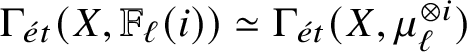 $\Gamma _{\acute {e}t}(X, \mathbb {F}_\ell (i)) \simeq \Gamma _{\acute {e}t}(X, \mu _\ell ^{\otimes i})$
for its étale version. If
$\Gamma _{\acute {e}t}(X, \mathbb {F}_\ell (i)) \simeq \Gamma _{\acute {e}t}(X, \mu _\ell ^{\otimes i})$
for its étale version. If
 $A = \mathbb {Z}[1/\ell , \zeta _\ell ]$
, then
$A = \mathbb {Z}[1/\ell , \zeta _\ell ]$
, then
 $H^0_{\acute {e}t}(A, \mathbb {F}_\ell ) = \mathbb {F}_\ell $
,
$H^0_{\acute {e}t}(A, \mathbb {F}_\ell ) = \mathbb {F}_\ell $
,
 $H^1_{\acute {e}t}(A, \mathbb {F}_\ell ) = A^\times /\ell $
and
$H^1_{\acute {e}t}(A, \mathbb {F}_\ell ) = A^\times /\ell $
and
 $H^*_{\acute {e}t}(A, \mathbb {F}_\ell ) = 0$
else; see [Reference Bachmann, Kong, Wang and Xu52, Remark II.2.2]. Corollary 8 implies that
$H^*_{\acute {e}t}(A, \mathbb {F}_\ell ) = 0$
else; see [Reference Bachmann, Kong, Wang and Xu52, Remark II.2.2]. Corollary 8 implies that
 $\Gamma (A, \mathbb {F}_\ell (i)) \simeq \Gamma _{\acute {e}t}(A, \mathbb {F}_\ell (i))_{\ge -i}$
. A transfer argument shows
$\Gamma (A, \mathbb {F}_\ell (i)) \simeq \Gamma _{\acute {e}t}(A, \mathbb {F}_\ell (i))_{\ge -i}$
. A transfer argument shows
 $\Gamma (\mathbb {Z}[1/\ell ], \mathbb {F}_\ell (i))$
is a summand of
$\Gamma (\mathbb {Z}[1/\ell ], \mathbb {F}_\ell (i))$
is a summand of
 $\Gamma (A, \mathbb {F}_\ell (i))$
, and similarly for
$\Gamma (A, \mathbb {F}_\ell (i))$
, and similarly for
 $\Gamma _{\acute {e}t}$
. We deduce the equivalence
$\Gamma _{\acute {e}t}$
. We deduce the equivalence
 $$ \begin{align*} \Gamma(\mathbb{Z}[1/\ell], \mathbb{F}_\ell(i)) \simeq \Gamma_{\acute{e}t}(\mathbb{Z}[1/\ell], \mathbb{F}_\ell(i))_{\ge -i}. \end{align*} $$
The same is true for
 $\mathbb C,\mathbb R,\mathbb {F}_p$
since they are Nisnevich local. Consequently, condition (1) will hold if the square
$\mathbb C,\mathbb R,\mathbb {F}_p$
since they are Nisnevich local. Consequently, condition (1) will hold if the square

is Cartesian and the maps
 $$ \begin{align*} H^i_{\acute{e}t}(\mathbb R, \mathbb{F}_\ell(i)) \oplus H^i_{\acute{e}t}(\mathbb{F}_p, \mathbb{F}_\ell(i)) \to H^i_{\acute{e}t}(\mathbb C, \mathbb{F}_\ell(i)) \end{align*} $$
are surjective for every i. The first condition holds by [Reference Röndigs, Spitzweck and Østvær24, Theorem 2.1]. The second condition is vacuous when
 $i>0$
and easily verified for
$i>0$
and easily verified for
 $i=0$
.
$i=0$
.
Remark 4.15. By adjoining an
 $\ell $
th root of unity, one obtains the commutative square
$\ell $
th root of unity, one obtains the commutative square

This induces a Cartesian square in étale cohomology but not in motivic cohomology (since, e.g., the group
 $H^{1,0}(\mathbb {Z}[1/\ell ,\zeta _\ell ],\mathbb {F}_\ell )=0$
but the corresponding map on
$H^{1,0}(\mathbb {Z}[1/\ell ,\zeta _\ell ],\mathbb {F}_\ell )=0$
but the corresponding map on
 $H^{0,0}$
is not surjective).
$H^{0,0}$
is not surjective).
4.3.4 Relation to étale homotopy types
Corresponding to the squares in Theorems 4.7, 4.11 and 4.14, there are analogous squares of étale homotopy types; in fact, Lemma 4.2, the only nonformal input in the construction of the said squares, also holds for étale homotopy types. Due to the equivalence
 $$ \begin{align*} \mathrm{H}_{\acute{e}t}\mathbb{Z}/{\ell^n} \simeq \mathrm{H}\mathbb{Z}/{\ell^n}[(\tau)^{-1}] \in \mathcal{SH}(S)_\ell^{\wedge\text{cell}} \end{align*} $$
from, for example, [Reference Washington9, Theorem 7.4], our co-Cartesian squares in
 $\mathcal {C\!M}_{\mathbb {Z}[1/\ell ]}$
induce Cartesian squares in étale cohomology with
$\mathcal {C\!M}_{\mathbb {Z}[1/\ell ]}$
induce Cartesian squares in étale cohomology with
 $\mathbb {Z}/{\ell ^n}(i)$
-coefficients. By Dwyer–Friedlander [Reference Röndigs, Spitzweck and Østvær24, Theorem 2.1] [Reference Dugger and Isaksen23, pp. 144–145], the resulting squares of étale homotopy types become pushouts after appropriate homological localisation.
$\mathbb {Z}/{\ell ^n}(i)$
-coefficients. By Dwyer–Friedlander [Reference Röndigs, Spitzweck and Østvær24, Theorem 2.1] [Reference Dugger and Isaksen23, pp. 144–145], the resulting squares of étale homotopy types become pushouts after appropriate homological localisation.
By analysing the proof of Theorem 4.14, one sees that condition (1) in Proposition 7 is satisfied if the following hold:
-
○
$\dim X_0 \le 1$
,
$\dim X_n = 0$
else. -
○ The induced square of étale cohomology with
$\mathbb {F}_\ell (i)$
-coefficients is Cartesian. -
○ The induced square of Zariski cohomology with
$\mathbb {F}_\ell $
-coefficients is Cartesian. -
○ The group
$H^1_{\mathrm {Zar}}(X_0, R^i \epsilon _* \mathbb {F}_\ell (i)) = 0$
for
$i \ge 0$
.


5 Applications to slice completeness and universal motivic invariants
We apply the results in Section 4 to show slice completeness and compute the endomorphism ring of the motivic sphere over regular number rings. Our completeness result for Voevodsky’s slice filtration [Reference Blumberg, Gepner and Tabuada72] is motivated by applications such as motivic generalisations of Thomason’s étale descent theorem for algebraic K-theory in [Reference Hoyois25] and [Reference Washington9], convergence of the slice filtration [Reference Jacobson45], the solution of Milnor’s conjecture on quadratic forms in [Reference Rognes and Østvær61], computations of universal motivic invariants in [Reference Elmanto, Levine, Spitzweck and Østvær64] and of hermitian K-groups in [Reference Hoyois43].
For the standard nomenclature associated with the slice filtration, such as the effective covers
 $f_{q}$
and the effective cocovers
$f_{q}$
and the effective cocovers
 $f^{q}$
, and the slice completion
$f^{q}$
, and the slice completion
 $\mathrm {sc}$
we refer to [Reference Voevodsky63, §3, (3.1), (3.3), (3.10)]. Let
$\mathrm {sc}$
we refer to [Reference Voevodsky63, §3, (3.1), (3.3), (3.10)]. Let
 $\mathcal {SH}(S)_{\ge 0}$
denote the connective motivic spectra with respect to the homotopy t-structure on
$\mathcal {SH}(S)_{\ge 0}$
denote the connective motivic spectra with respect to the homotopy t-structure on
 $\mathcal {SH}(S)$
[Reference Lurie36, §2.1]. The notion of a cell presentation of finite type is defined in [Reference Elmanto, Levine, Spitzweck and Østvær64, §3.3]. We shall say that a completeness property requiring a map
$\mathcal {SH}(S)$
[Reference Lurie36, §2.1]. The notion of a cell presentation of finite type is defined in [Reference Elmanto, Levine, Spitzweck and Østvær64, §3.3]. We shall say that a completeness property requiring a map
 $E \to F$
to be an equivalence holds ‘on homotopy’ if
$E \to F$
to be an equivalence holds ‘on homotopy’ if
 $\pi _{**} E \to \pi _{**} F$
is an isomorphism.
$\pi _{**} E \to \pi _{**} F$
is an isomorphism.
Proposition 11. Suppose F is a
 $2$
-regular number field and set
$2$
-regular number field and set
 ${\mathcal O}_{F}^{\prime }:= \mathcal O_F[1/2]$
.
${\mathcal O}_{F}^{\prime }:= \mathcal O_F[1/2]$
.
-
1. Let
$\mathcal {E}_\bullet \in \mathcal {SH}({\mathcal O}_{F}^{\prime })_2^{\wedge \text {cell}}$
be a tower such that
$\operatorname *{\mathrm {lim}}_n p_i^*(\mathcal {E}_n) \simeq 0$
, where
$p_i^*$
denotes the pullback to any of the fields in Theorem 4.7(1). Then
$\operatorname *{\mathrm {lim}}_n \mathcal {E}_n \simeq 0$
is contractible. -
2. If
$\mathcal {E} \in \mathcal {SH}({\mathcal O}_{F}^{\prime })^{\text {veff}} \cap \mathcal {SH}({\mathcal O}_{F}^{\prime })^{\text {cell}}$
is cellular and very effective, then
$\mathcal {E}/2$
is
$\eta $
-complete on homotopy. -
3. Let
$\mathcal {E} \in \mathcal {SH}({\mathcal O}_{F}^{\prime })_{\ge 0} \cap \mathcal {SH}({\mathcal O}_{F}^{\prime })^{\text {cell}}$
and assume the slices of
$\mathcal {E}$
are cellular and stable under base change. Then there is an isomorphism
$$ \begin{align*} \pi_{\ast,\ast}(\operatorname*{\mathrm{lim}}_n f^n(\mathcal{E})/(2,\rho)) \simeq \pi_{\ast,\ast}(\mathcal{E}/(2,\rho)). \end{align*} $$
-
4. Let
$\mathcal {E} \in \mathcal {SH}({\mathcal O}_{F}^{\prime })^{\mathrm{eff}}\cap \mathcal {SH}({\mathcal O}_{F}^{\prime })^{\mathrm{cell}}$
be cellular and effective. Assume
$\mathcal {E}/2$
has a
$\mathbb {Z}_{(2)}$
-cell presentation of finite type and its slices are cellular and stable under base change. Then
$\mathcal {E}/(2,\eta )$
is slice complete on homotopy and
$$ \begin{align*} \pi_{\ast,\ast}(\mathrm{sc}(\mathcal{E})_2^\wedge) \simeq \pi_{\ast,\ast}( \mathcal{E}_{2,\eta}^\wedge). \end{align*} $$


In particular, there is an isomorphism
 $$ \begin{align*} \pi_{\ast,\ast}(\mathrm{sc}(\mathbf{1})_2^\wedge)\simeq \pi_{\ast,\ast}(\mathbf{1}_2^\wedge). \end{align*} $$
Proof. (1) Let
 $I = \{* \to * \leftarrow *\}$
be the category so that
$I = \{* \to * \leftarrow *\}$
be the category so that
 $\operatorname *{\mathrm {lim}}_I$
means pullback. For all
$\operatorname *{\mathrm {lim}}_I$
means pullback. For all
 $X \in \mathcal {SH}({\mathcal O}_{F}^{\prime })_2^{\wedge \text {cell}}$
we compute
$X \in \mathcal {SH}({\mathcal O}_{F}^{\prime })_2^{\wedge \text {cell}}$
we compute
 $$ \begin{gather*} \mathrm{Map}(X, \operatorname*{\mathrm{lim}}_n \mathcal{E}_n) \simeq \operatorname*{\mathrm{lim}}_n \mathrm{Map}(X, \mathcal{E}_n) \simeq \operatorname*{\mathrm{lim}}_n \operatorname*{\mathrm{lim}}_{i \in I} \mathrm{Map}(p_i^*(X), p_i^*(\mathcal{E}_n)) \\ \simeq \operatorname*{\mathrm{lim}}_i \operatorname*{\mathrm{lim}}_n \mathrm{Map}(p_i^*(X), p_i^*(\mathcal{E}_n)) \simeq \operatorname*{\mathrm{lim}}_i \mathrm{Map}(p_i(X), \operatorname*{\mathrm{lim}}_n p_i^*(\mathcal{E}_n)) \simeq 0. \end{gather*} $$
The result follows.
(2) Recall that
 $\mathcal {E}$
is
$\mathcal {E}$
is
 $\eta $
-complete if and only if
$\eta $
-complete if and only if
 $$ \begin{align*} \operatorname*{\mathrm{lim}} \left[ \cdots \xrightarrow{\eta} \Sigma^{2,2} \mathcal{E} \xrightarrow{\eta} \Sigma^{1,1} \mathcal{E} \xrightarrow{\eta} \mathcal{E} \right] \simeq 0. \end{align*} $$
Thus, by (1) it suffices to check
 $p_i^*(\mathcal {E}/2)$
is
$p_i^*(\mathcal {E}/2)$
is
 $\eta $
-complete for each i, which holds by [Reference Artin and Mazur10, Theorem 5.1].
$\eta $
-complete for each i, which holds by [Reference Artin and Mazur10, Theorem 5.1].
(3) The claim holds if and only if
 $\operatorname *{\mathrm {lim}}_n f_n(\mathcal {E})/(2,\rho ) \simeq 0$
on homotopy groups or, equivalently, when computed in
$\operatorname *{\mathrm {lim}}_n f_n(\mathcal {E})/(2,\rho ) \simeq 0$
on homotopy groups or, equivalently, when computed in
 $\mathcal {SH}({\mathcal O}_{F}^{\prime })^{\text {cell}}$
. The assumptions imply
$\mathcal {SH}({\mathcal O}_{F}^{\prime })^{\text {cell}}$
. The assumptions imply
 $f_n(\mathcal {E}) \in \mathcal {SH}({\mathcal O}_{F}^{\prime })^{\text {cell}}$
and
$f_n(\mathcal {E}) \in \mathcal {SH}({\mathcal O}_{F}^{\prime })^{\text {cell}}$
and
 $p_i^* f_n \mathcal {E} \simeq f_n p_i^* \mathcal {E}$
. Hence, by (1) it suffices to note that
$p_i^* f_n \mathcal {E} \simeq f_n p_i^* \mathcal {E}$
. Hence, by (1) it suffices to note that
 $\operatorname *{\mathrm {lim}}_n f^n(p_i^* \mathcal {E})/(2,\rho ) \simeq p_i^*(\mathcal {E})/(2,\rho )$
owing to [Reference Artin and Mazur10, Proposition 5.2].
$\operatorname *{\mathrm {lim}}_n f^n(p_i^* \mathcal {E})/(2,\rho ) \simeq p_i^*(\mathcal {E})/(2,\rho )$
owing to [Reference Artin and Mazur10, Proposition 5.2].
(4) For the first statement we need to prove
 $\operatorname *{\mathrm {lim}}_n f_n(\mathcal {E}/(2,\eta )) \simeq 0$
on homotopy groups. As in (3), this reduces to the same statement over fields, which holds by [Reference Elmanto, Levine, Spitzweck and Østvær64, Proposition 3.49]. For the second statement we need to show
$\operatorname *{\mathrm {lim}}_n f_n(\mathcal {E}/(2,\eta )) \simeq 0$
on homotopy groups. As in (3), this reduces to the same statement over fields, which holds by [Reference Elmanto, Levine, Spitzweck and Østvær64, Proposition 3.49]. For the second statement we need to show
 $\mathrm {sc}(\mathcal {E}/2) \simeq \mathcal {E}_\eta ^\wedge /2$
, which holds by the proof of [Reference Elmanto, Levine, Spitzweck and Østvær64, Lemma 3.13]:
$\mathrm {sc}(\mathcal {E}/2) \simeq \mathcal {E}_\eta ^\wedge /2$
, which holds by the proof of [Reference Elmanto, Levine, Spitzweck and Østvær64, Lemma 3.13]:
 $\mathrm {sc}(\mathcal {E}/2)$
is
$\mathrm {sc}(\mathcal {E}/2)$
is
 $\eta $
-complete since
$\eta $
-complete since
 $\mathcal {E}/2$
is effective, and
$\mathcal {E}/2$
is effective, and
 $\mathrm {sc}(\mathcal {E}/2)/\eta \simeq \mathrm {sc}(\mathcal {E}/(2,\eta )) \simeq \mathcal {E}/(2,\eta )$
– the first equivalence holds by inspection of the slices. The final statement follows since the slices of
$\mathrm {sc}(\mathcal {E}/2)/\eta \simeq \mathrm {sc}(\mathcal {E}/(2,\eta )) \simeq \mathcal {E}/(2,\eta )$
– the first equivalence holds by inspection of the slices. The final statement follows since the slices of
 $\mathbf {1}_{(2)}$
over
$\mathbf {1}_{(2)}$
over
 ${\mathcal O}_{F}^{\prime }$
are known and have the desired properties by [Reference Elmanto, Levine, Spitzweck and Østvær64, Remark 2.2, Theorem 2.12].
${\mathcal O}_{F}^{\prime }$
are known and have the desired properties by [Reference Elmanto, Levine, Spitzweck and Østvær64, Remark 2.2, Theorem 2.12].
Remark 5.1. We expect that analogs of Proposition 11 hold over more general base schemes. Moreover, we expect that these results hold without the qualification ‘on homotopy’. Both shortcomings are a result of our specific technique for accessing global sections of cellular spectra over arithmetic base schemes.
Recall that any unit
 $a \in \mathcal O(S)^\times $
gives rise to a map
$a \in \mathcal O(S)^\times $
gives rise to a map
 $[a]: \mathbf {1} \to S^{1,1} \in \mathcal {SH}(S)$
and hence an element
$[a]: \mathbf {1} \to S^{1,1} \in \mathcal {SH}(S)$
and hence an element
 $$ \begin{align*} \langle a \rangle := 1 + \eta[a] \in \pi_{0,0}(\mathbf{1}_S). \end{align*} $$
This turns
 $\pi _{0,0}(\mathbf {1})$
into an
$\pi _{0,0}(\mathbf {1})$
into an
 $\mathbb {Z}[\mathcal O(S)^\times ]$
-algebra. We made use of the algebra structure in the formulation of Theorem 1.4 for
$\mathbb {Z}[\mathcal O(S)^\times ]$
-algebra. We made use of the algebra structure in the formulation of Theorem 1.4 for
 $\mathbb {Z}[1/2]$
. The generalisation to
$\mathbb {Z}[1/2]$
. The generalisation to
 $2$
-regular number rings takes the following form.
$2$
-regular number rings takes the following form.
Theorem 5.2. Suppose F is a
 $2$
-regular number field with r real embeddings and c pairs of complex embeddings. For the endomorphism ring of the motivic sphere over the base scheme
$2$
-regular number field with r real embeddings and c pairs of complex embeddings. For the endomorphism ring of the motivic sphere over the base scheme
 ${\mathcal O}_{F}^{\prime }:= \mathcal O_F[1/2]$
there is an isomorphism of
${\mathcal O}_{F}^{\prime }:= \mathcal O_F[1/2]$
there is an isomorphism of
 $\mathbb {Z}[({\mathcal O}_{F}^{\prime })^\times ]$
-algebras
$\mathbb {Z}[({\mathcal O}_{F}^{\prime })^\times ]$
-algebras
 $$ \begin{align*} \pi_{0,0}(\mathbf{1}_{{\mathcal O}_{F}^{\prime}}) \otimes \mathbb{Z}_{(2)} \simeq \mathrm{GW}({\mathcal O}_{F}^{\prime}) \otimes \mathbb{Z}_{(2)} \end{align*} $$
induced by the unit map
 $\mathbf {1} \to \mathrm {KO}$
. Moreover, we have the vanishing result
$\mathbf {1} \to \mathrm {KO}$
. Moreover, we have the vanishing result
 $$ \begin{align*} \pi_{*,0}(\mathbf{1}_{\mathcal O_F'}) \otimes \mathbb{Z}_{(2)} = 0. \quad\text{for}\quad *<0 \end{align*} $$
Proof. The presentation of Grothendieck–Witt rings of fields of characteristic
 $\neq 2$
by generators and relations given in [Reference Bachmann44, Theorem 4.1] implies there are
$\neq 2$
by generators and relations given in [Reference Bachmann44, Theorem 4.1] implies there are
 $\mathbb {Z}[({\mathcal O}_{F}^{\prime })^\times ]$
-algebra isomorphisms
$\mathbb {Z}[({\mathcal O}_{F}^{\prime })^\times ]$
-algebra isomorphisms
 $$ \begin{align*} \mathrm{GW}(\mathbb R) \simeq \mathbb{Z} \oplus \mathbb{Z}\{\langle -1 \rangle\}, \mathrm{GW}(\mathbb C) \simeq \mathbb{Z}, \mathrm{GW}(\mathbb{F}_q) \simeq \mathbb{Z} \oplus \mathbb{Z}/2. \end{align*} $$
In the isomorphism for
 $\mathrm {GW}(\mathbb {F}_q)$
, the right-hand side has trivial multiplication on the square class group
$\mathrm {GW}(\mathbb {F}_q)$
, the right-hand side has trivial multiplication on the square class group
 $\mathbb {F}_q^{\times }/(\mathbb {F}_q^{\times })^{2}\simeq \mathbb {Z}/2$
. As such, every n-dimensional form in
$\mathbb {F}_q^{\times }/(\mathbb {F}_q^{\times })^{2}\simeq \mathbb {Z}/2$
. As such, every n-dimensional form in
 $\mathrm {GW}(\mathbb {F}_q)$
can be written as either
$\mathrm {GW}(\mathbb {F}_q)$
can be written as either
 $n\langle 1\rangle $
or
$n\langle 1\rangle $
or
 $(n-1)\langle 1\rangle \oplus \langle a\rangle $
, where a is a nonsquare element in
$(n-1)\langle 1\rangle \oplus \langle a\rangle $
, where a is a nonsquare element in
 $\mathbb {F}_q^{\times }$
(we may choose
$\mathbb {F}_q^{\times }$
(we may choose
 $a=-1$
if and only if
$a=-1$
if and only if
 $q\equiv 3\bmod 4$
). Moreover, by [Reference Bökstedt15, Proposition 2.1(7)] and the proof of [Reference Dwyer and Friedlander13, Theorem 5.8], one deduces the
$q\equiv 3\bmod 4$
). Moreover, by [Reference Bökstedt15, Proposition 2.1(7)] and the proof of [Reference Dwyer and Friedlander13, Theorem 5.8], one deduces the
 $\mathbb {Z}[({\mathcal O}_{F}^{\prime })^\times ]$
-algebra isomorphism
$\mathbb {Z}[({\mathcal O}_{F}^{\prime })^\times ]$
-algebra isomorphism
 $$ \begin{align*} \mathrm{GW}({\mathcal O}_{F}^{\prime}) \simeq \mathbb{Z}^{1+r} \oplus (\mathbb{Z}/2)^{1+c}. \end{align*} $$
Thus, for the closed points
 $x, y_1, \dots , y_{c} \in \mathrm {Spec}({\mathcal O}_{F}^{\prime })$
in the notation of Theorem 4.7, there is a pullback square of
$x, y_1, \dots , y_{c} \in \mathrm {Spec}({\mathcal O}_{F}^{\prime })$
in the notation of Theorem 4.7, there is a pullback square of
 $\mathbb {Z}[({\mathcal O}_{F}^{\prime })^\times ]$
-algebras
$\mathbb {Z}[({\mathcal O}_{F}^{\prime })^\times ]$
-algebras

The Grothendieck–Witt rings appearing in (5.1) are quotients of
 $\mathbb {Z}[({\mathcal O}_{F}^{\prime })^\times ]$
. Thus, the maps in (5.1) are unique as
$\mathbb {Z}[({\mathcal O}_{F}^{\prime })^\times ]$
. Thus, the maps in (5.1) are unique as
 $\mathbb {Z}[({\mathcal O}_{F}^{\prime })^\times ]$
-algebra maps. Since
$\mathbb {Z}[({\mathcal O}_{F}^{\prime })^\times ]$
-algebra maps. Since
 $2$
-adic completion is exact on finitely generated abelian groups, this square remains Cartesian after
$2$
-adic completion is exact on finitely generated abelian groups, this square remains Cartesian after
 $2$
-adic completion.
$2$
-adic completion.
Consider the long exact sequence of homotopy groups associated with the pullback square

We have
 $\pi _{\ast ,0}(\mathbf {1}_2^\wedge )(\mathbb C) \simeq (\pi _*^s)_2^\wedge $
by [Reference Gabber46, Corollary 2]. It follows that the right vertical map in (5.2) is surjective on homotopy groups. Indeed, recall that
$\pi _{\ast ,0}(\mathbf {1}_2^\wedge )(\mathbb C) \simeq (\pi _*^s)_2^\wedge $
by [Reference Gabber46, Corollary 2]. It follows that the right vertical map in (5.2) is surjective on homotopy groups. Indeed, recall that
 $\mathcal {SH}^{fin}$
is the initial stable symmetric monoidal
$\mathcal {SH}^{fin}$
is the initial stable symmetric monoidal
 $\infty $
-category according to [Reference Weibel16, Theorem 3.1]. Thus, for any symmetric monoidal stable
$\infty $
-category according to [Reference Weibel16, Theorem 3.1]. Thus, for any symmetric monoidal stable
 $\infty $
-category
$\infty $
-category
 $\mathcal C$
and symmetric monoidal functor
$\mathcal C$
and symmetric monoidal functor
 $F: \mathcal C \to \mathcal {SH}(\mathbb C)_2^\wedge $
, there exists a factorisation
$F: \mathcal C \to \mathcal {SH}(\mathbb C)_2^\wedge $
, there exists a factorisation
 $$ \begin{align*} (\pi_{*}^s)_{2}^\wedge \to \pi_{*}(c_{2}^\wedge) \xrightarrow{F} \pi_{*,0}((\mathbf{1}_{\mathbb C})_{2}^\wedge) \end{align*} $$
and the composite is surjective by Levine’s result. Thus, using [Reference Milne55, Corollary 6.43], we deduce the pullback square of rings

Note that (5.3) comes from a diagram in
 $\mathcal {C\!M}_{{\mathcal O}_{F}^{\prime }}$
. Hence, the maps in (5.3) are
$\mathcal {C\!M}_{{\mathcal O}_{F}^{\prime }}$
. Hence, the maps in (5.3) are
 $\pi _{0,0}(\mathbf {1}_2^\wedge )({\mathcal O}_{F}^{\prime })$
-algebra maps, so a fortiori
$\pi _{0,0}(\mathbf {1}_2^\wedge )({\mathcal O}_{F}^{\prime })$
-algebra maps, so a fortiori
 $\mathbb {Z}[({\mathcal O}_{F}^{\prime })^\times ]$
-algebra maps. The Grothendieck–Witt rings in (5.3) are quotients of
$\mathbb {Z}[({\mathcal O}_{F}^{\prime })^\times ]$
-algebra maps. The Grothendieck–Witt rings in (5.3) are quotients of
 $\mathbb {Z}[({\mathcal O}_{F}^{\prime })^\times ]_2^\wedge $
; thus, the lower horizontal and right-hand vertical maps in (5.3) are unique
$\mathbb {Z}[({\mathcal O}_{F}^{\prime })^\times ]_2^\wedge $
; thus, the lower horizontal and right-hand vertical maps in (5.3) are unique
 $\mathbb {Z}[({\mathcal O}_{F}^{\prime })^\times ]$
-algebra maps. Thus, (5.3) is the
$\mathbb {Z}[({\mathcal O}_{F}^{\prime })^\times ]$
-algebra maps. Thus, (5.3) is the
 $2$
-adic completion of (5.2) and there is an isomorphism of
$2$
-adic completion of (5.2) and there is an isomorphism of
 $\mathbb {Z}[({\mathcal O}_{F}^{\prime })^\times ]$
-algebras
$\mathbb {Z}[({\mathcal O}_{F}^{\prime })^\times ]$
-algebras
 $$ \begin{align*} \pi_{0,0}(\mathbf{1}_2^\wedge)({\mathcal O}_{F}^{\prime}) \simeq \mathrm{GW}({\mathcal O}_{F}^{\prime})_2^\wedge. \end{align*} $$
There is a similar pullback square for
 $\pi _{1,0}(\mathord -) \otimes \mathbb {Q}$
. Since the vanishing
$\pi _{1,0}(\mathord -) \otimes \mathbb {Q}$
. Since the vanishing
 $\pi _{1,0}(\mathbf {1}_2^\wedge )(k) \otimes \mathbb {Q} = 0$
holds for
$\pi _{1,0}(\mathbf {1}_2^\wedge )(k) \otimes \mathbb {Q} = 0$
holds for
 $k = \mathbb R$
[Reference Morel21, Figure 4],
$k = \mathbb R$
[Reference Morel21, Figure 4],
 $k=\mathbb C$
[Reference Gabber46, Corollary 2] and
$k=\mathbb C$
[Reference Gabber46, Corollary 2] and
 $k=\mathbb {F}_q$
[Reference Wilson and Østvær75, Theorem 1.3], we deduce the vanishing
$k=\mathbb {F}_q$
[Reference Wilson and Østvær75, Theorem 1.3], we deduce the vanishing
 $$ \begin{align*} \pi_{1,0}(\mathbf{1}_2^\wedge)({\mathcal O}_{F}^{\prime}) \otimes \mathbb{Q} = 0. \end{align*} $$
Inserted into the fracture square long exact sequence we get a pullback square of
 $\mathbb {Z}[({\mathcal O}_{F}^{\prime })^\times ]$
-algebras
$\mathbb {Z}[({\mathcal O}_{F}^{\prime })^\times ]$
-algebras

By inspection there are isomorphisms of
 $\mathbb {Z}[({\mathcal O}_{F}^{\prime })^\times ]$
-algebras
$\mathbb {Z}[({\mathcal O}_{F}^{\prime })^\times ]$
-algebras
 $$ \begin{align*} \pi_{0,0}(\mathbf{1})({\mathcal O}_{F}^{\prime}) \otimes \mathbb{Q} & \simeq H^0_{r\acute{e}t}({\mathcal O}_{F}^{\prime},\mathbb{Q}) \times H^0({\mathcal O}_{F}^{\prime},\mathbb{Q}) \\ &\simeq \mathbb{Q}^{r} \times \mathbb{Q} \\ &\simeq \mathrm{GW}({\mathcal O}_{F}^{\prime}) \otimes \mathbb{Q}. \end{align*} $$
We refer to [Reference Isaksen7, Theorem 7.2] for a proof of the first isomorphism. Since
 $\pi _{0,0}(\mathbf {1})({\mathcal O}_{F}^{\prime }) \otimes \mathbb {Q}$
is a quotient of
$\pi _{0,0}(\mathbf {1})({\mathcal O}_{F}^{\prime }) \otimes \mathbb {Q}$
is a quotient of
 $\mathbb {Z}[({\mathcal O}_{F}^{\prime })^\times ] \otimes \mathbb {Q}$
, in (5.4), the right-hand vertical map
$\mathbb {Z}[({\mathcal O}_{F}^{\prime })^\times ] \otimes \mathbb {Q}$
, in (5.4), the right-hand vertical map
 $$ \begin{align*} \pi_{0,0}(\mathbf{1})({\mathcal O}_{F}^{\prime}) \otimes \mathbb{Q} \simeq \mathrm{GW}({\mathcal O}_{F}^{\prime}) \otimes \mathbb{Q} \to \pi_{0,0}(\mathbf{1}_2^\wedge)({\mathcal O}_{F}^{\prime}) \otimes \mathbb{Q} \simeq \mathrm{GW}({\mathcal O}_{F}^{\prime})_2^\wedge \otimes \mathbb{Q} \end{align*} $$
is the unique
 $\mathbb {Z}[({\mathcal O}_{F}^{\prime })^\times ]$
-algebra map. This shows we can identify the square of
$\mathbb {Z}[({\mathcal O}_{F}^{\prime })^\times ]$
-algebra map. This shows we can identify the square of
 $\mathbb {Z}[({\mathcal O}_{F}^{\prime })^\times ]$
-algebras (5.4) with the corresponding fracture square for
$\mathbb {Z}[({\mathcal O}_{F}^{\prime })^\times ]$
-algebras (5.4) with the corresponding fracture square for
 $\mathrm {GW}({\mathcal O}_{F}^{\prime })\otimes \mathbb {Z}_{(2)}$
. It also follows that the unit map to
$\mathrm {GW}({\mathcal O}_{F}^{\prime })\otimes \mathbb {Z}_{(2)}$
. It also follows that the unit map to
 $\mathrm {KO}$
induces an isomorphism, since
$\mathrm {KO}$
induces an isomorphism, since
 $\pi _{0,0}(\mathrm {KO}_{\mathcal O_F}) = \mathrm {GW}(\mathcal O_F')$
is a quotient of
$\pi _{0,0}(\mathrm {KO}_{\mathcal O_F}) = \mathrm {GW}(\mathcal O_F')$
is a quotient of
 $\mathbb {Z}[\mathcal O_F^{\prime \times }]$
.
$\mathbb {Z}[\mathcal O_F^{\prime \times }]$
.
Next we show the vanishing
 $\pi _{*,0}(\mathbf {1}_{\mathcal O_F'}) \otimes \mathbb {Z}_{(2)} = 0$
for
$\pi _{*,0}(\mathbf {1}_{\mathcal O_F'}) \otimes \mathbb {Z}_{(2)} = 0$
for
 $*<0$
. From (5.2), since a is surjective on
$*<0$
. From (5.2), since a is surjective on
 $\pi _*$
and all terms except possibly the top left vanish on
$\pi _*$
and all terms except possibly the top left vanish on
 $\pi _*$
for
$\pi _*$
for
 $*<0$
, we deduce that
$*<0$
, we deduce that
 $\pi _{*,0}((\mathbf {1}_{\mathcal O_F'})_2^\wedge ) = 0$
for
$\pi _{*,0}((\mathbf {1}_{\mathcal O_F'})_2^\wedge ) = 0$
for
 $*<0$
. Since
$*<0$
. Since
 $\mathrm {GW}(\mathcal O_F')$
is finitely generated, the map
$\mathrm {GW}(\mathcal O_F')$
is finitely generated, the map
 $$ \begin{align*} \mathrm{GW}(\mathcal O_F') \otimes \mathbb{Q} \times \mathrm{GW}(\mathcal O_F')_2^\wedge \to \mathrm{GW}(\mathcal O_F')_2^\wedge \otimes \mathbb{Q} \end{align*} $$
is surjective. Considering the fracture square for
 $\pi _{*,0}(\mathbf {1}_{\mathcal O_F'}) \otimes \mathbb {Z}_{(2)}$
, it thus remains to prove
$\pi _{*,0}(\mathbf {1}_{\mathcal O_F'}) \otimes \mathbb {Z}_{(2)}$
, it thus remains to prove
 $\pi _{*,0}(\mathbf {1}_{\mathcal O_F'}) \otimes \mathbb {Q} = 0$
for
$\pi _{*,0}(\mathbf {1}_{\mathcal O_F'}) \otimes \mathbb {Q} = 0$
for
 $*<0$
. This follows from the identification of these groups with subquotients of the rational gamma filtration and rational real étale cohomology, both of which vanish in these degrees, as above.
$*<0$
. This follows from the identification of these groups with subquotients of the rational gamma filtration and rational real étale cohomology, both of which vanish in these degrees, as above.
Applying the same proof method establishes the following odd-primary analog of Theorem 5.2.
Theorem 5.3. Let
 $\ell $
be an odd prime number. Suppose F is
$\ell $
be an odd prime number. Suppose F is
 $\ell $
-regular and
$\ell $
-regular and
 $\mu _{\ell }\subset F$
. For the endomorphism ring of
$\mu _{\ell }\subset F$
. For the endomorphism ring of
 $\mathbf {1}_{{\mathcal O}_{F}^{\prime }}$
over the base scheme
$\mathbf {1}_{{\mathcal O}_{F}^{\prime }}$
over the base scheme
 ${\mathcal O}_{F}^{\prime }:= \mathcal O_F[1/\ell ]$
there is an isomorphism of
${\mathcal O}_{F}^{\prime }:= \mathcal O_F[1/\ell ]$
there is an isomorphism of
 $\mathbb {Z}[({\mathcal O}_{F}^{\prime })^\times ]$
-algebras
$\mathbb {Z}[({\mathcal O}_{F}^{\prime })^\times ]$
-algebras
 $$ \begin{align*} \pi_{0,0}(\mathbf{1}_{{\mathcal O}_{F}^{\prime}}) \otimes \mathbb{Z}_{(\ell)} \simeq \mathrm{GW}({\mathcal O}_{F}^{\prime}) \otimes \mathbb{Z}_{(\ell)}. \end{align*} $$
Moreover, we have the vanishing result
 $$ \begin{align*} \pi_{*,0}(\mathbf{1}_{\mathcal O_F'}) \otimes \mathbb{Z}_{(\ell)} = 0 \quad\text{for}\quad *<0. \end{align*} $$
The same results hold for the motivic sphere over the base scheme
 $\mathbb {Z}[1/\ell ]$
when
$\mathbb {Z}[1/\ell ]$
when
 $\ell $
is a regular prime.
$\ell $
is a regular prime.
Acknowledgments
We acknowledge the support of the Centre for Advanced Study at the Norwegian Academy of Science and Letters in Oslo, Norway, which funded and hosted our research project ‘Motivic Geometry’ during the 2020/21 academic year. We thank the anonymous referees for their valuable comments. This research was supported by grants from the RCN Frontier Research Group Project no. 250399 ‘Motivic Hopf Equations’ and no. 312472 ‘Equations in Motivic Homotopy’.
Conflict of Interest
None.


 Open access