


1. Introduction
Gromov–Witten theory is a crucial part of one side of mirror symmetry. It can be encoded as a statement about a generating function of Gromov–Witten invariants. As we may guess, a function generated by genus  $0$ (‘ $g=0$’ for short) invariants only is relatively easier to study than one with all invariants. Interestingly, it recovers higher-genus invariants in some cases [Reference Givental11], and may be of independent interest.
The J-function is the first-order derivative of the  $g=0$ generating function. We will see its precise definition and various other descriptions in the following section and Section 2.1. The I-function is known to be a counterpart of the J-function in mirror symmetry. From mirror symmetry it follows that the I-function appears as a solution of differential equations which has a beautiful presentation as a hypergeometric series. This description can be used in several applications of the study of $g=0$ Gromov–Witten theory. However, in spite of the importance of the I-function, it is difficult to compute the differential equations whose solution it is, and further it does not have a concrete definition.
In [Reference Givental10], Givental described the I-function for a toric complete intersection as a generating function of invariants defined by integrations on certain moduli spaces. Inspired by Givental’s idea, Ciocan-Fontanine, Kim and Maulik constructed quasimap moduli spaces for a GIT quotient [Reference Ciocan-Fontanine, Kim and Maulik7], which suggested a concrete definition of the I-function in greater generality [Reference Ciocan-Fontanine and Kim6]. One advantage of this approach is that one can study the I-function without knowledge of the mirror. The purpose of this article is to construct moduli spaces generalising the results to a fibre bundle with GIT quotient fibres.
Meanwhile, the relationship between I- and J-functions is highly nontrivial, even if we know what the I-function should be. That relationship is called the mirror conjecture/theorem. Various mirror theorems have been proved since the seminal breakthrough by Givental [Reference Givental10]. In [Reference Brown4], Brown proved the mirror theorem for a fibre bundle whose fibre is a toric variety, thus proving a conjecture of Elezi’s [Reference Elezi9] (see our Conjecture 1 and Theorem 4). Note that Elezi’s conjecture was about projective bundles. Brown’s result is in fact stronger than the original conjecture. His proof does not use moduli spaces to establish the conjecture. The main purpose of this article is to prove the mirror theorem for fibre bundles whose fibre is a flag variety using moduli spaces.
1.1. Gromov–Witten invariants
Before explaining further, we would like to review Gromov–Witten invariants for a smooth projective variety X over  $\mathbb {C}$. Roughly, Gromov–Witten invariants count morphisms from curves to X passing through given subvarieties of X. To be precise, we consider a collection of such morphisms
 $$ \begin{align} \mathcal{M}_{g,k}(X, \beta) := \{ (C,f) \}\ / \sim_{isom}, \end{align} $$
where
• C is a smooth curve of genus g with k marked and
• $f: C \rightarrow X$ is of degree $\beta \in H_2(X,\mathbb {Z})$,
together with the evaluation maps
 $$ \begin{align*}\mathrm{ev}_a:{\mathcal{M}}_{g,k}(X , \beta) \rightarrow X, \qquad (C, p_1, \ldots, p_k, f: C \rightarrow X) \mapsto f(p_a) \end{align*} $$
at the marked points. Denoting by  $X_a \in H^*(X, \mathbb {Q}[\![q]\!])$ the Poincaré dual of the ath given subvariety, the invariant can be thought of as an intersection number
 $$ \begin{align*}\deg\left( \left[{\mathcal{M}}_{g,k}(X, \beta)\right] \cap \prod_{a=1}^k \mathrm{ev}_a^*(X_a) \right) = \int_{\left[{\mathcal{M}}_{g,k}\left(X, \beta\right)\right]} \prod_{a=1}^k \mathrm{ev}_a^*(X_a). \end{align*} $$
 A problem is that the space (1.1.1) may not be compact, and thus the intersection number may not be defined. Using stable maps, we can compactify the space (1.1.1). The result is a Deligne–Mumford (DM) stack, usually denoted by  $\overline {\mathcal {M}}_{g,k}(X, \beta )$. Another problem is that it may not be smooth, and thus its fundamental class may not have the expected dimension. However, $\overline {\mathcal {M}}_{g,k}(X, \beta )$ is equipped with a natural perfect obstruction theory, so that its virtual fundamental class $\left [\overline {\mathcal {M}}_{g,k}(X, \beta )\right ]^{vir}$ is defined. Gromov–Witten invariant is then defined by
 $$ \begin{align*}\int_{\left[\overline{\mathcal{M}}_{g,k}\left(X, \beta\right)\right]^{vir}} \prod_{a=1}^k \mathrm{ev}_a^*(X_a). \end{align*} $$
1.2. $g=0$ Gromov–Witten theory

The second homology classes  $\beta $ defining nonempty $\overline {\mathcal {M}}_{g,k}(X, \beta )$ form a monoid in $H_2(X,\mathbb {Z})$. We denote it by $\mathrm {Eff}(X)$, or $\mathrm {Eff}$ for short. One can define the group ring
 $$ \begin{align*}{\mathbb Q}[\![q]\!] := \mathbb{Q}[\![\mathrm{Eff}]\!] = \left\langle q^{\beta} \ \middle | \ \beta \in \mathrm{Eff}\right \rangle, \end{align*} $$
called the Novikov ring. The psi class  $\psi _a$ is defined as the first Chern class of the line bundle on $\overline {\mathcal {M}}_{g,k}(X , \beta )$ formed by cotangent lines of C at $p_a$. Then the $g=0$ descendant potential of X is defined by
 $$ \begin{align*}\mathcal{F}_0 := \sum_{k=0}^{\infty} \sum_{\beta \in \mathrm{Eff}} \frac{q^{\beta}}{k!} \int_{\left[\overline{\mathcal{M}}_{0,k}\left(X, \beta\right)\right]^{vir}} \prod_{a=1}^k \sum_{n=0}^{\infty} \mathrm{ev}_a^*(t_n)\psi_a^n, \end{align*} $$
where  $t_0, t_1, \ldots \in H^*(X, \mathbb {Q}[\![q]\!])$ are formal variables. The function ${\mathcal {F}}_0$ is one key ingredient of mirror symmetry. For instance, mirror symmetry predicts that the quantum cohomology ring of X is isomorphic to the Jacobian ring of its mirror. Setting $t_0 := \sum _i t^i\gamma ^i$ for a basis $\left \{\gamma ^i\right \}$ of $H^*(X)$ with the dual basis $\{\gamma _i\}$, the quantum cohomology is defined by $\left (H^*\left (X, \mathbb {Q}[\![q]\!]\right ), \star _{t_0}\right )$ with the product
 $$ \begin{align*}\gamma^i \star_{t_0} \gamma^j = \partial_{t^i}\partial_{t^j}\partial_{t^k} \mathcal{F}_0\rvert_{t_1=t_2=\cdots=0} \cdot \gamma_k. \end{align*} $$
Note that the restriction to  $q=t_0=0$ of the quantum cohomology is the usual cohomology.
The Lagrangian cone  ${\mathcal {L}} ag_X$ of $g=0$ Gromov–Witten theory of X is roughly defined as the graph of the differential (in an infinite dimensional vector space)
 $$ \begin{align*}{\mathcal{L}} ag_X := \Gamma\left(d{\mathcal{F}}_0 \right) \subset T^{\vee}_{H^*\left(X, \mathbb{Q}\right)[z] \otimes_{\mathbb Q} {\mathbb Q}[\![q]\!]}, \end{align*} $$
(see [Reference Coates and Givental8, Reference Givental12] for the precise definition). It is an origin-shifted cone in the vector space. Using the (nontrivial) identification of symplectic spaces
 $$ \begin{align*}T^{\vee}_{H^*\left(X, \mathbb{Q}\right)[z] \otimes_{\mathbb Q} {\mathbb Q}[\![q]\!]} \cong \left( H^*(X, \mathbb{Q})[z] \oplus \frac{1}{z}H^*(X, \mathbb{Q})\left[\!\left[z^{-1}\right]\!\right] \right) \otimes_{\mathbb Q} {\mathbb Q}[\![q]\!] =: {\mathcal{H}}, \end{align*} $$
its shifting  $-z^{-1} {\mathcal {L}} ag_X$ is spanned by the derivatives of (the $z^{-1}$-expansion of) the J-function $J_X(-z, {\textbf t})$ [Reference Coates and Givental8, Proposition 1], where $J_{X}(z, {\textbf t})$ is
 $$ \begin{align} 1 + \frac{{\textbf t}}{z} + \sum_{ \left(k,\beta\right) \neq \left(0,0\right),\left(1,0\right)} \frac{q^{\beta}}{k!} (\mathrm{ev}_{k+1})_*\left(\frac{\prod_{a=1 }^{k}\mathrm{ev}_a^*({\textbf t})\left[\overline{\mathcal{M}}_{0,k+1}(X, \beta)\right]^{vir}}{z(z - \psi_{k+1})} \right). \end{align} $$
 Computing  $J_X$ is very difficult in general, but mirror symmetry predicts that it is related to a different, often more computable function known as the I-function. A modern form of the mirror conjecture/theorem (introduced by Givental) is to prove that an I-function lies on the Lagrangian cone. This then allows one to recover the J-function via a complicated procedure of Birkhoff factorisation and change of variables.
1.3. Mirror theorem
When X is a GIT quotient  $X = V /\!\!/ {\textbf G}$, there is a nice description of the I-function $I_X$ [Reference Ciocan-Fontanine, Kim and Maulik7, Reference Ciocan-Fontanine and Kim6]. Ciocan-Fontanine, Kim and Maulik constructed another compactification $Q_{g,k}(X,\beta )$ of the space (1.1.1) by allowing morphisms $C \rightarrow [V/{\textbf G}]$ taking the generic point to X. These are called quasimaps. Then the I-function is defined by
 $$ \begin{align*}I_{X}(z, \textbf{t}) := \sum_{ \left(k,\beta\right) } \frac{q^{\beta}}{k!} (\mathrm{ev}_{k+1})_*\left(\frac{\prod_{a=1 }^{k}\mathrm{ev}_a^*(\textbf{t})\left[Q_{0,k+1}(X, \beta)\right]^{vir}}{e_{{\mathbb C}^*}\left(N_{k,\beta}^{vir}\right)} \right), \end{align*} $$
where  $N_{k,\beta }^{vir}$ denotes the virtual normal bundle of $Q_{0,k+1}(X, \beta )$ to a ‘graph quasimap space’ (see equation (2.1.5) and Proposition 6 for graph spaces and virtual normal bundles). The input variable z is the equivariant parameter of ${\mathbb C}^*$.
When a torus acts on X, Ciocan-Fontanine and Kim proved the mirror theorem which is a generalisation of the result by Givental [Reference Givental10] for a complete intersection X in a toric variety.
In [Reference Brown4], Brown defined the I-function for a fibre bundle whose fibre is a toric variety and proved the mirror theorem (see Theorem 4).
1.4. The main result
The main goal of this article is to define the I-function and prove the mirror theorem for  $X ={\mathcal {F}}^{(n)}$, a fibre bundle over a smooth projective variety Y whose fibre is a partial flag variety.
We start with F the total space of a sum of line bundles  $\oplus _{j=1}^r L_j $ on Y and the n-tuple of positive integers
 $$ \begin{align*}(r_1, \ldots, r_n) \in {\mathbb Z}^n, \quad 0< r_1 < \cdots <r_n<r_{n+1}:=r. \end{align*} $$
Then we let  $\pi : \mathcal {F}^{(n)} \rightarrow Y$ be a fibre bundle over Y whose fibre at $y \in Y$ is the space of all collections of subspaces
 $$ \begin{align*} F_1 \subset F_2 \subset \cdots \subset F_n \subset F\rvert_y, \qquad \mathrm{rank} F_i=r_i. \end{align*} $$
Our plan is to write the I-function in terms of J-function of Y and the I-function of the fibre. So let
 $$ \begin{align*}{\mathbb Q}[\![Q]\!] := {\mathbb Q}[\![\mathrm{Eff}(Y)]\!] \end{align*} $$
be the Novikov ring of Y and  $J_{D}$ be the $Q^{D}$-coefficient of $J_Y$. With a formal variable $u \in H^*(Y, \mathbb {Q})$, we can write
 $$ \begin{align*}J_Y (z, u) = \sum_{D} Q^{D} J_{D}(z ,u).\end{align*} $$
Let  $\mathcal {F}_1 \subset \cdots \subset \mathcal {F}_n \subset \mathcal {F}_{n+1}:= \pi ^*F$ be the tautological bundles on $\mathcal {F}^{(n)}$. For an effective class $D \in \mathrm {Eff}(Y)$, let ${\mathbb Z}^n_D$ be the collection of all $\beta \in \mathrm {Eff}\left ({\mathcal {F}}^{(n)}\right )$ satisfying $\pi _*\beta =D$. Then ${\mathbb Z}^n_D$ is a subset of ${\mathbb Z}^n$ via $\beta \mapsto \left (\beta \left (\det {\mathcal {F}}^{\vee }_i\right )\right )_i \in {\mathbb Z}^n$. Furthermore, $\cup _{D \in \mathrm {Eff}(Y)} \left ( \{D\} \times {\mathbb Z}^n_D \right )$ forms a monoid in $\mathrm {Eff}(Y) \times {\mathbb Z}^n$, since so does $\mathrm {Eff}\left ({\mathcal {F}}^{(n)}\right )$. Let ${\mathbb Q}[\![q,Q]\!]$ be the group ring defined by the monoid. It is the Novikov ring of ${\mathcal {F}}^{(n)}$, and ${\mathbb Q}[\![q,Q]\!] \rightarrow {\mathbb Q}[\![Q]\!]$ is induced by the projection of the monoid to $\mathrm {Eff}(Y)$. Let $H_{i,l}$ be Chern roots of $\mathcal {F}_i^{\vee }$, $i=1, \ldots , n$, $l=1, \ldots , r_i$ and $H_{n+1,j}:= -\pi ^*\left (c_1\left (L_j\right )\right )$. Then for formal variables $\textbf {t} = \sum _{i=1}^n t_i c_1\left ({\mathcal {F}}_i ^{\vee }\right ) \in H^{ 2}\left (\mathcal {F}^{(n)}, \mathbb {Q} \right )$ and $u \in H^*(Y, \mathbb {Q})$, we define the I-function for ${\mathcal {F}}^{(n)}$:
 $$ \begin{align} I_{{\mathcal{F}}^{(n)}} (z, {\textbf{t}}, u) & := e^{\frac{\textbf{t}}{z}} \sum_{D \in \mathrm{Eff}(Y), d= \left(d_i\right) \in {\mathbb Z}^n_D} q^d Q^D e^{\sum_i t_i d_i} \pi^*(J_{D}(z, u)) \\ & \quad \times \sum_{\sum_l d_i^l =d_i} \prod_{i=1}^n \left( \prod_{1 \leq l \neq l' \leq r_i}\frac{\prod_{s=-\infty}^{d_i^l -d_i^{l'}}\left(H_{i,l}-H_{i,l'}+sz\right) }{\prod_{s=-\infty}^{0}\left(H_{i,l}-H_{i,l'}+sz\right)} \right. \nonumber \\ & \quad \times \left. \prod_{1 \leq l \leq r_i, 1 \leq l' \leq r_{i+1}}\frac{\prod_{s=-\infty}^{0}\left(H_{i,l}-H_{i+1,l'}+sz\right)}{\prod_{s=-\infty}^{d_i^l -d_{i+1}^{l'}}\left(H_{i,l}-H_{i+1,l'}+sz\right)} \right), \nonumber \end{align} $$
which is an element in  ${\mathcal {H}}$, where $d^j_{n+1}:= - c_1\left (L_j\right ) \cap D = - D\left (L_j\right )$. The summation over $\sum _i d^l_i = d_i$ is taken as follows. Note that in Section 4.2 we will express ${\mathcal {F}}^{(n)}$ as a quotient $E /\!\!/ {\textbf G}$ of a vector bundle E on Y by a linearly reductive group $\textbf G$. The term $\left (d^l_i\right )$ in formula (1.4.3) is an effective class of its abelianisation $E /\!\!/ {\textbf G}_T$, where ${\textbf G}_T$ is a maximal torus of ${\textbf G}$, whose image under the push-forward of the stack morphism $[E/{\textbf G}_T] \to [E/ {\textbf G}]$ is $d_i$. Hence the summation is finite.
Here is our main result:
Theorem 1. The I-function  $I_{{\mathcal {F}}^{(n)}}(-z, {\textbf {t}}, u)$ lies on $-z^{-1}\mathcal {L}ag_{\mathcal {F}^{(n)}}$.
1.5. Equivariant theory
We prove Theorem 1 using a natural fibrewise action of a torus  $\textbf {S} := ({\mathbb C}^*)^r$ on ${\mathcal {F}}^{(n)}$. Let $\lambda $ be the equivariant parameters of $\textbf S$. The action defines the $\textbf {S}$-equivariant I-function for ${\mathcal {F}}^{(n)}$, denoted by $I^{\textbf {S}}_{{\mathcal {F}}^{(n)}} (z, {\textbf {t}},u, \lambda )$. Theorem 1 follows from its equivariant version by taking $\lambda \rightarrow 0$.
Theorem 2. The I-function  $I^{\textbf {S}}_{{\mathcal {F}}^{(n)}}( -z, {\textbf {t}}, u, \lambda )$ lies on $-z^{-1}{\mathcal {L}} ag^{\textbf {S}}_{{\mathcal {F}}^{(n)}}$.
We prove Theorem 2 through a characterisation of  ${\mathcal {L}} ag ^{\textbf {S}} _{{\mathcal {F}}^{(n)}}$ (Theorem 3). The characterisation determines whether or not a function
 $$ \begin{align*}G \in {\mathcal{H}} [\![{\textbf t}, u]\!] \subset H^*_{\textbf S} \left({\mathcal{F}}^{(n)}, {\mathbb Q}\right)(z) \otimes_{\mathbb Q} {\mathbb Q}[\![q, Q, {\textbf t}, u]\!] \end{align*} $$
lies on  $-z^{-1}{\mathcal {L}} ag ^{\textbf {S}} _{{\mathcal {F}}^{(n)}}[\![{\textbf t}, u]\!]$. Here, for a rational function in z we consider its $z^{-1}$-expansion when we need to view it as a series.
Theorem 3. Suppose that G has the following properties:
1. the initial condition in Section 2.2.1,
2. the recursion relation in Section 2.2.2 and
3. the polynomiality condition in Section 2.2.3.
Then  $G(-z, {\textbf t}, u, \lambda )$ lies on $-z^{-1}{\mathcal {L}} ag^{\textbf {S}} _{{\mathcal {F}}^{(n)}}$ at each ${\textbf t}$ and u.
1.6. Plan of the paper
We explain properties in Section 2.2 and prove Theorem 3 in Section 2.4. A brief strategy is as follows. We first produce a function, say F, associated with G which lies on the Lagrangian cone. Then we show  $G=F$ using the characterisation properties for G. In Section 2.3 we discuss a converse of Theorem 3.
We will show that  $I^{\textbf S}_{{\mathcal {F}}^{(n)}}$ satisfies the characterisation properties in Sections 3 and 5. In Section 3 we will compute the residues at some simple poles to check that equation (2.2.7) holds for the I-function. The quasimap spaces are introduced and studied in Section 4, which is quite independent from other sections. Then we write $I^{\textbf {S}}_{{\mathcal {F}}^{(n)}}$ in terms of the quasimap spaces and check the properties for it using the geometric interpretation in Section 5.
As an application of our main result, in Section 6 we show how the  $g = 0$ Gromov–Witten invariants of the base and total space are related to each other when ${\mathcal {F}}^{(n)}$ is assumed to be Fano or Calabi–Yau.
1.7. Relationship to previous works: What is new and what is not
When  $Y = \mathrm {Spec} \mathbb {C}$, Theorem 1 specialises a result by Bertram, Ciocan-Fontanine and Kim [Reference Bertram, Ciocan-Fontanine and Kim2, Reference Bertram, Ciocan-Fontanine and Kim3]. When $n=r_1=1$, Theorem 1 proves Elezi’s conjecture [Reference Elezi9] as a special case.
Conjecture 1 Elezi [Reference Elezi9]
Let  $L_1 := {\mathcal {O}}_Y$ and $L_j$, $j \neq 1$, be nef line bundles on Y such that $-K_Y -\sum _j c_1\left (L_j\right )$ is ample. Then we have
 $$ \begin{align*}I_{{\mathbb P}\left(\oplus_{j=1}^r L_j\right)} = J_{{\mathbb P}\left(\oplus_{j=1}^r L_j\right)}. \end{align*} $$
 In [Reference Brown4], Brown proves Elezi’s conjecture. He considers a toric fibration  $\pi : \mathcal {T}:=\oplus _{j=1}^r L_j /\!\!/ (\mathbb {C}^*)^n \rightarrow Y$, $n \leq r$. It has r many toric divisors
 $$ \begin{align*}D_j := \oplus_{i \neq j} L_i /\!\!/ (\mathbb{C}^*)^n \subset \mathcal{T} \end{align*} $$
and n many line bundles  $P_i$ corresponding to the ith factor of the torus $({\mathbb C}^*)^n$. For ${\textbf t}=\sum _{i=1}^n t_i c_1(P_i)$, he defined the I-function
 $$ \begin{align*} \begin{array}{c} I_{{\mathcal{T}}} (z, {\textbf t}, u) := e^{\frac{\textbf t}{z}} \displaystyle\sum_{\beta \in \mathrm{Eff}} q^{\beta} e^{\int_{\beta} {\textbf t}} \pi^*\left(J_{\pi_*(\beta)}(z, u)\right) \prod_{j=1}^r \frac{\prod_{s=-\infty}^{0}\left(D_j +sz\right)}{\prod_{s=-\infty}^{D_j.\beta}\left(D_j +sz\right)}. \\ \end{array} \end{align*} $$
Theorem 4 Brown [Reference Brown4]
The I-function  $I_{{\mathcal {T}}}(-z, {\textbf t}, u)$ lies on $-z^{-1}\mathcal {L}ag_{\mathcal {T}}$.
For Theorem 4, Brown also used a characterisation [Reference Brown4, Theorem 2]. His characterisation has a fairly different aspect from ours because he used an asymptotic analysis to check whether the I-function satisfies the characterisation properties, whereas we will check it using the geometric interpretation of the I-function.
Our characterisation is motivated by [Reference Givental10, Proposition 4.5] and [Reference Ciocan-Fontanine and Kim6, Lemma 7.7.1]. Essentially, both assert that a function satisfying the recursion relation in Section 2.2.2 and the polynomiality condition in Section 2.2.3 lies on the Lagrangian cone.
In [Reference Givental10, Reference Ciocan-Fontanine and Kim6], the I-functions were interpreted in terms of suitable moduli spaces. The recursion and the polynomiality were checked by virtual localisation [Reference Graber and Pandharipande13].
1.7.1. Characterisation properties
Since our target space is a fibre bundle over  $Y \neq {\mathrm {Spec}} {\mathbb C}$, the recursion and polynomiality used in [Reference Givental10, Reference Ciocan-Fontanine and Kim6] for $Y = {\mathrm {Spec}} {\mathbb C}$ are not enough. So they need to be modified. Since the recursion relation is a recursive argument with respect to the fibre direction, we need an initial condition of that recursive argument in terms of the base space Y. This is the reason why the initial condition in Section 2.2.1 is imposed on the characterisation theorem. The polynomiality condition should be extended to any directional derivative along a vector at the origin on the cohomology of Y; see formula (2.2.8) for the precise statement. These modifications are newly designed.
1.7.2. Quasimap moduli spaces
For a construction of moduli spaces, we have to keep two things in mind. First, the invariants of such moduli spaces produce  $I^{\textbf S}_{{\mathcal {F}}^{(n)}}$ as a generating function. Second, the construction must be natural enough to check the characterisation properties for $I^{\textbf S}_{{\mathcal {F}}^{(n)}}$ easily.
An immediate approach to the construction might be a direct generalisation of [Reference Givental10, Reference Ciocan-Fontanine and Kim6] – constructing a space of maps which project prestable maps to the base Y and quasimaps [Reference Ciocan-Fontanine, Kim and Maulik7] to the fibre. However, this approach is not good enough to meet the first purpose. So we will introduce a new idea which considers a space of maps which project prestable maps to Y and quasimaps from contracted domain curves to the fibre. In Section 4, we formalise this construction.
Remark 1. In Section 3, we will compute residues in the recursion relation without using moduli spaces. But this computation can be done by virtual localisation as well.
2. Characterisation theorem
In this section, we would like to explain characterisation properties and prove Theorem 3. Since it characterises elements in the Lagrangian cone which is generated by the J-function, we start with a study of that function.
Indeed, though the characterisation can be generalised to any fibre bundle with a nice fibrewise torus action, we prefer to focus on  ${\mathcal {F}}^{(n)}$.
2.1. J-function
We have seen the definition of the J-function in formula (1.2.2). Its equivariant version  $J^{\textbf {S}}_{{\mathcal {F}}^{(n)}}$ is described in the same way. Meanwhile, there is an alternative expression of $J^{\textbf {S}}_{{\mathcal {F}}^{(n)}}$ providing a geometric meaning for the variable z. Consider the so-called graph space
 $$ \begin{align} \overline{{\mathcal{M}}}G_{0,k}\left({\mathcal{F}}^{(n)}, \beta\right) := \overline{\mathcal{M}}_{0,k}\left({\mathcal{F}}^{(n)} \times \mathbb{P}^1, (\beta,1)\right). \end{align} $$
Then the  $\mathbb {C}^*$-action on $\mathbb {P}^1$,
 $$ \begin{align*}{\mathbb C}^* \times {\mathbb P}^1 \rightarrow {\mathbb P}^1, \qquad (t,[x;y]) \mapsto [tx;y], \end{align*} $$
defines an action on  $\overline {\mathcal {M}}G_{0,k}\left ({\mathcal {F}}^{(n)} , \beta \right )$. If we set the convention $0=[0;1]$, $\infty =[1;0]$, then we obtain
 $$ \begin{align*}e_{{\mathbb C}^*}\left(T_0 {\mathbb P}^1\right)=z ,\qquad e_{{\mathbb C}^*}\left(T_{\infty} {\mathbb P}^1\right)=-z, \end{align*} $$
where  $z=e_{{\mathbb C}^*}({\mathbb C}_1)$ is the Euler class of the $1$-dimensional ${\mathbb C}^*$-representation with weight $1$. On the domain curve for an element in $\overline {{\mathcal {M}}}G_{0,k}\left ({\mathcal {F}}^{(n)}, \beta \right )$, there is the unique rational component ${\mathbb P}^1$ which identically maps to the ${\mathbb P}^1$-factor on the target space. We call this component on the domain curve the distinguished ${\mathbb P}^1$. By abuse of notation, we will denote this component simply by ${\mathbb P}^1$ when there is no danger of confusion. Let $F_{k,\beta } \subset \overline {\mathcal {M}}G_{0,k}\left ({\mathcal {F}}^{(n)} , \beta \right )^{\mathbb {C}^*}$ be a component of the ${\mathbb C}^*$-fixed locus, where $\infty \in {\mathbb P}^1$ is neither a marked point nor a node. There is an isomorphism $F_{k,\beta } \cong \overline {{\mathcal {M}}}_{0,k+1}\left ({\mathcal {F}}^{(n)}, \beta \right )$, unless $(k,\beta ) = (0,0), (1,0)$, defined by contracting ${\mathbb P}^1$ to the extra marked point. We call it the distinguished marked point. Since ${\mathbb P}^1$ maps constantly to ${\mathcal {F}}^{(n)}$, we can define an evaluation map $\mathrm {ev}_{\bullet }: F_{k,\beta } \rightarrow {\mathcal {F}}^{(n)}$ by the constant image of ${\mathbb P}^1$. It is $\mathrm {ev}_{\bullet } = \mathrm {ev}_{k+1}$ through the isomorphism $F_{k,\beta } \cong \overline {{\mathcal {M}}}_{0,k+1}\left ({\mathcal {F}}^{(n)}, \beta \right )$ if $(k,\beta ) \neq (0,0), (1,0)$. Hence $J^{\textbf {S}}_{{\mathcal {F}}^{(n)}}$ (formula (1.2.2)) can be rewritten as
 $$ \begin{align} J^{\textbf{S}}_{{\mathcal{F}}^{(n)}}(\textbf{t}) = \displaystyle\sum_{ k,\beta} \frac{q^{\beta}}{k!} (\mathrm{ev}_{\bullet})_*\left(\frac{\prod_{a=1}^{k}\mathrm{ev}_a^*(\textbf{t})\left[F_{k,\beta}\right]^{vir}}{e_{{\mathbb C}^* \times {\textbf{S}}}\left(N^{vir}_{F_{k,\beta}/ \overline{\mathcal{M}}G_{0,k}\left({\mathcal{F}}^{(n)}, \beta\right)}\right)} \right), \end{align} $$
where  $N^{vir}$ denotes the virtual normal bundle with respect to the ${\mathbb C}^*$-action. The term $q^{\beta } \in {\mathbb Q}\left [\!\left [\mathrm {Eff}\left ({\mathcal {F}}^{(n)}\right )\right ]\!\right ]$ can be thought of as $q^{\left (\beta \left (\det {\mathcal {F}}^{\vee }_i\right )\right )_i}Q^{\pi _*\beta } \in {\mathbb Q}[\![q,Q]\!]$ under the isomorphism ${\mathbb Q}\left [\!\left [\mathrm {Eff}\left ({\mathcal {F}}^{(n)}\right )\right ]\!\right ] \cong {\mathbb Q}[\![q,Q]\!]$. Note that for $(k,\beta ) \neq (0,0), (1,0)$, we have
 $$ \begin{align*}e_{{\mathbb C}^* \times {\textbf{S}}}\left(N^{vir}_{F_{k,\beta}/ \overline{\mathcal{M}}G_{0,k}\left({\mathcal{F}}^{(n)}, \beta\right)}\right) = z(z-\psi_{\bullet})\end{align*} $$
from the contributions of moving and smoothing the nodal point  $\bullet =0 \in {\mathbb P}^1$.
There is one more useful description of the J-function. We define an operator
 $$ \begin{align*} & S^*_{\textbf t}(z): H^*_{\textbf{S}}\left({{\mathcal{F}}^{(n)}}, {\mathbb Q}\right)[z] \otimes_{\mathbb Q} {\mathbb Q}[\![ q]\!] \rightarrow H^*_{\textbf{S}}\left({{\mathcal{F}}^{(n)}}, {\mathbb Q}\right)(z) \otimes_{\mathbb Q} {\mathbb Q}[\![ q]\!], \\ & \gamma \mapsto \gamma + \sum_{\left(m,\beta\right) \neq \left(0,0\right)} \frac{q^{\beta}}{m!} (\mathrm{ev}_1)_* \left( \frac{\mathrm{ev}_2^*(\gamma)\prod_{i=1}^m \mathrm{ev}_{i+2}^*({\textbf{t}})\left[\overline{{\mathcal{M}}}_{0,2+m}\left({{\mathcal{F}}^{(n)}}, \beta\right)\right]^{vir}}{z-\psi_1}\right). \end{align*} $$
Letting  $\{\gamma _i\}$ be a basis for $H^*_{\textbf {S}}\left ({{\mathcal {F}}^{(n)}}, {\mathbb Q} \right )$ and $t_i$ be a formal variable corresponding to $\gamma _i$, one can check that $S^*_{\textbf {t}}(z)(\gamma _i) = z\partial _{t_i} J^{\textbf {S}}_{{\mathcal {F}}^{(n)}}$ using formula (1.2.2). On the other hand, by [Reference Coates and Givental8, Proposition 1(i)], we have
 $$ \begin{align*}T_f {\mathcal{L}} \cap {\mathcal{L}} ag_{{\mathcal{F}}^{(n)}} = zT_f {\mathcal{L}}\end{align*} $$
at any point  $f \in {\mathcal {L}} ag_{{\mathcal {F}}^{(n)}}$, where $T_f {\mathcal {L}}$ denotes the tangent space to ${\mathcal {L}} ag_{{\mathcal {F}}^{(n)}}$ at f. Hence any directional derivative $z\partial f$ lies on $zT_f {\mathcal {L}} \subset \mathcal {L}ag_{{\mathcal {F}}^{(n)}}$. Applying it to $f=-zJ^{\textbf S}_{{\mathcal {F}}^{(n)}}(-z)$, one can check that $S^*_{\textbf {t}}(-z)(\gamma )$ lies on $-z^{-1}{\mathcal {L}} ag^{\textbf S}_{{\mathcal {F}}^{(n)}}$ for any $\gamma $. For the special case $\gamma =1$, we have
 $$ \begin{align} S^*_{\textbf{t}}(z)(1) = J^{\textbf{S}}_{{\mathcal{F}}^{(n)}} \end{align} $$
by the string equation of Gromov–Witten theory [Reference Givental12, (SE)]. Conversely,  $\left \{S^*_{\textbf {t}}(-z)(\gamma _i)\right \}_i$ spans $T_{-zJ^{\textbf S}_{{\mathcal {F}}^{(n)}}(-z)}{\mathcal {L}}$ as a free ${\mathbb Q}[\![q]\!][z]$-module [Reference Coates and Givental8, Proposition 1]. This property is called the reconstruction of the Lagrangian cone.
2.2. Characterisation properties
Now we explain characterisation properties for a function
 $$ \begin{align*}G \in {\mathcal{H}} [\![{\textbf t}, u]\!] \subset H^*_{\textbf S} \left({\mathcal{F}}^{(n)}, {\mathbb Q}\right)(z) \otimes_{\mathbb Q} {\mathbb Q}[\![q, Q, {\textbf t}, u]\!]. \end{align*} $$
Note that the J-function (formulas (1.2.2), (2.1.5) and (2.1.6)) is defined on the whole cohomology  ${\textbf t} \in H^*\left ({\mathcal {F}}^{(n)}, {\mathbb Q}\right )$, whereas G is the function on the restriction $H^2\left ({\mathcal {F}}^{(n)}, {\mathbb Q}\right ) \oplus H^*(Y, {\mathbb Q}) \subset H^*\left ({\mathcal {F}}^{(n)}, {\mathbb Q}\right )$. By abuse of notation, we use $\textbf t$ for the variable on $H^2\left ({\mathcal {F}}^{(n)}, {\mathbb Q}\right )$; u denotes the variable on $H^*(Y, {\mathbb Q})$.
2.2.1. Initial condition
Let  $\mu : Y \hookrightarrow {\mathcal {F}}^{(n)}$ be the inclusion of an $\textbf {S}$-fixed locus. We denote its image by $Y^{\mu }:= \mu (Y)$. In [Reference Coates and Givental8], the $N_{Y^{\mu } / {\mathcal {F}}^{(n)}}$-twisted Gromov–Witten theory on $Y \cong Y^{\mu }$ is defined using the pairing
 $$ \begin{align*}\int_Y e^{-1}_{\textbf S} \left(N_{Y^{\mu} / {\mathcal{F}}^{(n)}} \right) a \cup b , \quad a, b \in H^*_{\textbf S}(Y) \cong H^*(Y)[\lambda]. \end{align*} $$
This gives rise to the twisted Lagrangian cone  ${\mathcal {L}}^{\mu }_Y$ [Reference Coates and Givental8, Section 7–10].
Denoting by  $G^{\mu } := \sum _{\left (d,D\right )} q^dQ^D \ G^{\mu }_{\left (d,D\right )}$ the pullback $\mu ^*G$, we define
 $$ \begin{align*}G^{\mu}_Y := \sum_{D} Q^D G^{\mu}_{\left(d_{D,\mu},D\right)}, \quad d_{D, \mu} := \left(D\left(\det \mu^*{\mathcal{F}}_i^{\vee}\right)\right)_i \in {\mathbb Z}^n. \end{align*} $$
The initial condition for G asserts that
•
$G\rvert _{q=Q=0}=e^{\left ({\textbf t} + \pi ^*u\right )/z}$ and•
$G^{\mu }_Y(-z, {\textbf t}, u)$ lies on $-z^{-1}{\mathcal {L}}^{\mu }_Y$.


2.2.2. Recursion relation
Let  $\mu , \nu : Y \hookrightarrow {\mathcal {F}}^{(n)}$ be $\textbf {S}$-fixed loci in ${\mathcal {F}}^{(n)}$ such that there exists a $1$-dimensional orbit connecting $Y^{\mu }$ and $Y^{\nu }$. Then for each point in $Y^{\mu }$, there is a unique $1$-dimensional orbit connecting this point to a point in $Y^{\nu }$. The tangent space to a $1$-dimensional orbit at each point in $Y^{\mu }$ forms an $\textbf S$-equivariant line bundle on $Y \cong Y^{\mu }$. Let
 $$ \begin{align*} \chi_{\mu,\nu} \in H^2_{\textbf S}(Y , {\mathbb Q}), \qquad d_{\mu,\nu} \in \mathrm{Eff}\left({\mathcal{F}}^{(n)}\right), \end{align*} $$
be, respectively, its first Chern class and the class of a representative of the  $1$-dimensional orbit.
For each integer  $k>0$, since $Y^{\mu } \cong Y$, we have an embedding $Y \hookrightarrow \overline {{\mathcal {M}}}_{0,2}\left ({\mathcal {F}}^{(n)}, kd_{\mu ,\nu }\right )^{\textbf {S}}$ defined by the k-coverings of orbits. Note that the two marked points correspond to $0, \infty \in {\mathbb P}^1$, the poles of orbits. Let
 $$ \begin{align*} N^{vir}_{\mu,\nu,k} := N^{vir}_{Y/ \overline{{\mathcal{M}}}_{0,2}\left({\mathcal{F}}^{(n)}, kd_{\mu,\nu}\right)} \end{align*} $$
be the virtual normal bundle to Y in  $\overline {{\mathcal {M}}}_{0,2}\left ({\mathcal {F}}^{(n)}, kd_{\mu ,\nu }\right )$.
We say that G satisfies the recursion relation if each coefficient of  $G^{\mu }$, as a series in q, Q, $\textbf {t}$ and u, has
• finite-order poles at
$z=0$ and $z=\infty $ and• simple poles at
$z=-\chi _{\mu ,\nu }/k$ for $k \in {\mathbb N}$, with residues given by (2.2.7)$$ \begin{align} {\mathrm{Res}}_{z=-\frac{\chi_{\mu,\nu}}{k}} G^{\mu}(z)dkz = \frac{q^{kd_{\mu,\nu}}}{e_{\textbf{S}}\left(N^{vir}_{\mu,\nu,k}\right)} e_{\textbf{S}}\left(N_{Y^{\mu} / {\mathcal{F}}^{(n)}}\right) G^{\nu} \left(-\frac{\chi_{\mu, \nu}}{k}\right). \end{align} $$


2.2.3. Polynomiality condition
Let  $\left \{\delta _j\right \}$ be a basis for $H^*(Y, {\mathbb Q})$ and $u_j$ be the corresponding variable in $u= \sum _j u_j \delta _j \in H^*(Y, {\mathbb Q})$. Also let $E_{i,\mu } := \det {\mathcal {F}}^{\vee }_{i} \otimes \pi ^*\mu ^* \det {\mathcal {F}}_{i} $ be the bundle on ${\mathcal {F}}^{(n)}$. Then the polynomiality condition for G says that
• for each
$\mu $ and j, the rational function (2.2.8)has no poles in$$ \begin{align} \left(z\partial_{u_j} G^{\mu}(z,q) , G^{\mu}\left(-z, qe^{-z\sum_i y_iE_{i,\mu}} \right) \right)_Y \end{align} $$$z =0$, where $y_i$s are formal variables.


2.3. Converse of Theorem 3
The J-function  $J^{\textbf S}_{{\mathcal {F}}^{(n)}}$ satisfies the initial condition $\big ($by [Reference Brown4, Theorem 2] and the reconstruction of ${\mathcal {L}}^{\mu }_Y\big )$ and the recursion relation [Reference Brown4, Reference Ciocan-Fontanine and Kim6, Reference Givental10]).
Proposition 1.  $J^{\textbf S}_{{\mathcal {F}}^{(n)}}$ satisfies the polynomiality condition as well.
Proof. Recall from equation (2.1.5) that  $J^{\textbf S}_{{\mathcal {F}}^{(n)}}$ is a summation of the integrations over $F_{k,\beta }$s. The term $F_{k,\beta }$ is a component in $\overline {{\mathcal {M}}}G_{0,k+1}\left ({\mathcal {F}}^{(n)}, \beta \right )^{{\mathbb C}^*}$. We consider other components
 $$ \begin{align*}F_{k_1,\beta_1}^{k_2,\beta_2} \subset \overline{{\mathcal{M}}}G_{0,k+1}\left({{\mathcal{F}}^{(n)}}, \beta\right)^{{\mathbb C}^*}, \quad k_1 +k_2=k, \quad \beta_1 + \beta_2 = \beta, \end{align*} $$
where  $k_1$-marked points, of degree $\beta _1$, are concentrated on $0=[1;0] \in \mathbb {P}^1$ and $k_2$-marked points, of degree $\beta _2$, are concentrated on $\infty \in \mathbb {P}^1$. Note that
 $$ \begin{align} F_{k_1,\beta_1}^{k_2,\beta_2} \cong F_{k_1,\beta_1} \times_{{\mathcal{F}}^{(n)}} F_{k_2, \beta_2}. \end{align} $$
Let  $\overline {{\mathcal {M}}}G_{0,k+1}\left ({{\mathcal {F}}^{(n)}}, \beta \right )_{\mu }$ be the $\textbf {S}$-fixed locus in $\overline {{\mathcal {M}}}G_{0,k+1}\left ({{\mathcal {F}}^{(n)}}, \beta \right )$ consisting of objects for which the image of $\mathbb {P}^1$ lies on $Y^{\mu } \subset \left ({{\mathcal {F}}^{(n)}}\right )^{\textbf {S}}$. Let $\left (F_{k_1,\beta _1}^{k_2,\beta _2}\right )_{\mu }$ be the substack of $F_{k_1,\beta _1}^{k_2,\beta _2}$ taking the marked point to $Y^{\mu }$.
With these spaces, a short strategy of the proof is as follows. Following the idea in [Reference Ciocan-Fontanine and Kim6, Section §7.6], we express the function (2.2.8) for  $G=J^{\textbf S}_{{\mathcal {F}}^{(n)}}$ as a sum of the integrations over $\overline {{\mathcal {M}}}G_{0,k+1}\left ({{\mathcal {F}}^{(n)}}, \beta \right )_{\mu }$s (see equation (2.3.15)). This seems reasonable because the latter (the right-hand side of equation (2.3.15)) is a sum of the integrations over $\left (F_{k_1,\beta _1}^{k_2,\beta _2}\right )_{\mu }$s by virtual localisation. On the other hand, it is equal to the former (the left-hand side of equation (2.3.15)) due to the isomorphism (2.3.9) and equation (2.1.5) for $J^{\textbf S}_{{\mathcal {F}}^{(n)}}$. Then, since $\overline {{\mathcal {M}}}G_{0,k+1}\left ({{\mathcal {F}}^{(n)}}, \beta \right )_{\mu }$ is an $\textbf S$-fixed locus, not a ${\mathbb C}^*$-fixed locus, the latter is a polynomial in the ${\mathbb C}^*$-equivariant parameter. In other words, it does not have a pole in $z=0$.
For each class  $\beta $ and $i=1, \ldots , n$, we would like to construct a $\mathbb {C}^* \times \textbf {S}$-equivariant line bundle $E_{i,\beta }$ on $\overline {{\mathcal {M}}}G_{0,k+1}\left ({\mathcal {F}}^{(n)}, \beta \right )$ such that
 $$ \begin{align} E_{i,\beta}\rvert_{F_{k_1 ,\beta_1}^{k_2, \beta_2}} = \mathrm{ev}^*_{\bullet} \left(\det {\mathcal{F}}_i^{\vee} \otimes \pi^*{\mathcal{O}}_{Y}(1)\right)\otimes \mathbb{C}_{\beta_2 \left(\det {\mathcal{F}}_i^{\vee} \otimes \pi^* {\mathcal{O}}_{Y}(1)\right)}, \end{align} $$
where  $\mathbb {C}_{\star }$ denotes the ${\mathbb C}^*$-representation of weight $\star $. Using the $\textbf S$-bundle $\det {\mathcal {F}}_i^{\vee } \otimes \pi ^* {\mathcal {O}}_{Y}(1)$, we obtain an $\textbf S$-morphism $\iota _i: {\mathcal {F}}^{(n)} \rightarrow {\mathbb P}^{N_i}$ for some $N_i$ (which may not be an embedding). It induces an $\textbf S$-morphism
 $$ \begin{align} \overline{{\mathcal{M}}}G_{0,k+1}\left({\mathcal{F}}^{(n)}, \beta\right) \longrightarrow \overline{{\mathcal{M}}}G_{0,k+1}\left({\mathbb P}^{N_i}, \iota_{i*}\beta\right). \end{align} $$
It automatically becomes a  ${\mathbb C}^*$-morphism as well by the definition of the graph spaces (2.1.4). By forgetting marked points, contracting all components except for the distinguished ${\mathbb P}^1$ on the domain curve and replacing contracted points on ${\mathbb P}^1$ with base points with the same degrees as the contracted components [Reference Ciocan-Fontanine and Kim6, eq(3.2.3)], we obtain a morphism
 $$ \begin{align} \overline{{\mathcal{M}}}G_{0,k+1}\left({\mathbb P}^{N_i}, \iota_{i*}\beta\right) \longrightarrow {\mathbb P}\left(\left({\mathrm{Sym}}^{\iota_{i*}\beta}H^0\left({\mathbb P}^1, {\mathcal{O}}_{{\mathbb P}^1}(1)\right)\right)^{\oplus {N_i+1}}\right). \end{align} $$
In [Reference Ciocan-Fontanine and Kim6, eq(3.2.3)], this morphism is written as
 $$ \begin{align*}G_{0,k+1,\iota_{i*}\beta}\left({\mathbb P}^{N_i}\right) \longrightarrow QG_{0,k+1,\iota_{i*}\beta}\left({\mathbb P}^{N_i}\right). \end{align*} $$
It is just a notational difference; they are exactly the same [Reference Ciocan-Fontanine and Kim6, Section §3.3,  ${2}^{\mathrm{nd}}$eq]. The quasimap moduli space (in the sense of [Reference Ciocan-Fontanine, Kim and Maulik7])
 $$ \begin{align*}QG_{0,k+1,\iota_{i*}\beta}\left({\mathbb P}^{N_i}\right) = {\mathbb P}\left(\left({\mathrm{Sym}}^{\iota_{i*}\beta}H^0\left({\mathbb P}^1, {\mathcal{O}}_{{\mathbb P}^1}(1)\right)\right)^{\oplus {N_i+1}}\right) \end{align*} $$
is a compactification of a space of morphisms of degree  $\iota _{i*}\beta \in {\mathbb Z}$ from ${\mathbb P}^1$ to ${\mathbb P}^{N_i}$ by allowing base points. The line bundle $E_{i,\beta }$ is defined as the pullback of the dual tautological bundle of the projective space by the map (2.3.12) $\circ $ (2.3.11). See [Reference Ciocan-Fontanine and Kim6, Section §3.3] for a more detailed construction; equation (2.3.10) is explained in [Reference Ciocan-Fontanine and Kim6, eq(5.2.1)].
Using  $\pi ^* \left ( \left (\det {\mathcal {F}}_i^{\vee }\right )\middle \rvert _{Y^{\mu }} \otimes \mathcal {O}_{Y}(1) \right )$, we can construct a $\mathbb {C}^* \times \textbf {S}$-line bundle $E_{i,\beta ,\mu }$ on $\overline {{\mathcal {M}}}G_{0,k+1}\left ({\mathcal {F}}^{(n)}, \beta \right )$ in the same way. Indeed, the construction comes through the forgetful (and stabilisation) morphism
 $$ \begin{align*}\overline{{\mathcal{M}}}G_{0,k+1}\left({\mathcal{F}}^{(n)}, \beta\right) \rightarrow \overline{{\mathcal{M}}}G_{0,k+1}(Y, \pi_*\beta). \end{align*} $$
Then the restriction of  $E_{i,\beta ,\mu }$ is
 $$ \begin{align} E_{i,\beta,\mu}\rvert_{F_{k_1 ,\beta_1}^{k_2, \beta_2}} = \mathrm{ev}^*_{\bullet} \pi^*\left(\mu^* \det {\mathcal{F}}_i^{\vee} \otimes \mathcal{O}_{Y}(1)\right)\otimes \mathbb{C}_{\pi_*\beta_2 \left(\mu^* \det {\mathcal{F}}_i^{\vee} \otimes \mathcal{O}_{Y}(1)\right)}. \end{align} $$
 Then setting  ${\mathcal {E}}_{i,\beta , \mu } := E_{i, \beta } \otimes E^{\vee }_{i,\beta ,\mu }$, we obtain by equations (2.3.10) and (2.3.13) that
 $$ \begin{align} {\mathcal{E}}_{i,\beta,\mu}\rvert_{F_{k_1 ,\beta_1}^{k_2, \beta_2} \cap \overline{{\mathcal{M}}}G_{0,k+1}\left({{\mathcal{F}}^{(n)}}, \beta\right)_{\mu}} = \mathbb{C}_{\beta_2 \left(\det {\mathcal{F}}_i^{\vee}\right) +\pi_*\beta_2\left( \mu^*\det {\mathcal{F}}_i \right)} = {\mathbb C}_{\beta_2\left(E_{i,\mu}\right)}. \end{align} $$
Let
 $$ \begin{align*}N^{vir}_{\mu} := N^{vir}_{\overline{{\mathcal{M}}}G_{0,k+1}\left({{\mathcal{F}}^{(n)}}, \beta\right)_{\mu}/\overline{{\mathcal{M}}}G_{0,k+1}\left({{\mathcal{F}}^{(n)}}, \beta\right)} \end{align*} $$
be the virtual normal bundle with respect to the  $\textbf S$-action. By abuse of notation, we set $q^{\beta } := q^dQ^D$ for $\beta =(d,D)$ and ${\textbf t} := {\textbf t} + \pi ^*u$, and consider
 $$ \begin{align*} Z_{\mu} := \sum_{k,\beta \geq 0} \frac{q^{\beta}}{k!} \frac{\left[\overline{{\mathcal{M}}}G_{0,k+1}\left({{\mathcal{F}}^{(n)}}, \beta\right)_{\mu}\right]^{vir}}{e_{{\mathbb C}^* \times \textbf{S}}\left(N^{vir}_{\mu}\right)} \cap e^{\sum_i c_1\left({\mathcal{E}}_{i,\beta, \mu} \right)y_i} \prod_{a=1}^k \mathrm{ev}_{a}^* (\textbf{t}) \mathrm{ev}_{k+1}^*\left(p_0\pi^* \delta_j\right), \end{align*} $$
where  $p_0 := e_{{\mathbb C}^*}({\mathcal {O}}(1) \otimes {\mathbb C}_1) \in H^*_{{\mathbb C}^*}\left ({\mathbb P}^1\right )$, so $p_0\rvert _0 = z$ and $p_0\rvert _{\infty } = 0.$ Recall from Section 2.2.3 that $\{\delta _i\}$ is a basis for $H^*(Y, {\mathbb Q})$ corresponding to the variables $\{u_i\}$. We observe that $Z_{\mu }$ has no poles in $z=0$, because each factor of the denominator has a nontrivial $\lambda $-term.
For the morphism  $\mathrm {pt}: \overline {{\mathcal {M}}}G_{0,k}\left ({{\mathcal {F}}^{(n)}}, \beta \right )_{\mu } \rightarrow {\mathrm {Spec}} {\mathbb C}$ to the point, we prove that
 $$ \begin{align} \left(z\partial_j J^{{\textbf{S}},\mu}_{{\mathcal{F}}^{(n)}}(z,q), J^{{\textbf{S}},\mu}_{{\mathcal{F}}^{(n)}}\left(-z,qe^{-z \sum_i y_iE_i }\right) \right)_Y = (\mathrm{pt})_*Z_{\mu}, \end{align} $$
using virtual  ${\mathbb C}^*$-localisation [Reference Graber and Pandharipande13]. The fixed loci are a disjoint union of $\left (F_{k_1, \beta _1}^{k_2,\beta _2}\right )_{\mu }$s. By abuse of notation, we denote by $N^{vir}$ the virtual normal bundle to $\left (F_{k_1, \beta _1}^{k_2,\beta _2}\right )_{\mu }$ in $\overline {{\mathcal {M}}}G_{0,k+1}\left ({{\mathcal {F}}^{(n)}}, \beta \right )$. Then we obtain
 $$ \begin{align*} Z_{\mu} = \sum_{k,\beta \geq 0} \sum_{\substack{k_1 +k_2 =k \\ \beta_1 +\beta_2=\beta}} \frac{q^{\beta}}{k!} \frac{\left[\left(F_{k_1 ,\beta_1}^{k_2, \beta_2}\right)_{\mu}\right]^{vir}}{e_{{\mathbb C}^* \times \textbf{S}}\left(N^{vir}\right)} \cap e^{\sum_i c_1\left({\mathcal{E}}_{i,\beta,\mu} \right)y_i} \prod_{a=1}^k \mathrm{ev}_{a}^* (\textbf{t}) \mathrm{ev}_{k+1}^*\left(p_0\pi^* \delta_j\right). \end{align*} $$
By equation (2.3.14) and the projection formula, we obtain  $\mathrm {pt}_*$ for each term
 $$ \begin{align*} &(\mathrm{pt})_* \frac{q^{\beta}}{k!} \frac{\left[\left(F_{k_1 ,\beta_1}^{k_2, \beta_2}\right)_{\mu}\right]^{vir}}{e_{{\mathbb C}^* \times \textbf{S} }\left(N^{vir}\right)} \cap e^{\sum_i c_1\left({\mathcal{E}}_{i,\beta, \mu} \right)y_i} \prod_{a=1}^k \mathrm{ev}_{a}^* (\textbf{t}) \mathrm{ev}_{k+1}^*\left(p_0\pi^* \delta_j\right) \\ &\qquad= \frac{q^{\beta}}{k!} e^{ z\sum_i y_i \beta_2\left(E_{i,\mu}\right) } \int_{\left[F_{k_1 ,\beta_1}^{k_2, \beta_2}\right]^{vir}} \frac{(\mathrm{ev}_{\bullet})^*\left( PD\left(Y_{\mu}\right)\right)}{e_{\mathbb{C}^* \times {\textbf S}}\left(N^{k_2 ,\beta_2}_{k_1, \beta_1}\right)} \prod_{a=1}^k \mathrm{ev}_{a}^* (\textbf{t}) \mathrm{ev}_{k+1}^*\left(p_0\pi^* \delta_j\right), \end{align*} $$
where  $N^{k_2,\beta _2}_{k_1,\beta _1} := N^{vir}_{F^{k_2,\beta _2}_{k_1,\beta _1}/\overline {{\mathcal {M}}}G_{0,k+1}\left ({{\mathcal {F}}^{(n)}}, \beta \right )}$ and $PD$ stands for ‘Poincaré dual’. Setting $N^{vir}_{k,\beta } := N^{vir}_{F_{k,\beta }/\overline {{\mathcal {M}}}G_{0,k}\left ({{\mathcal {F}}^{(n)}}, \beta \right )}$ and letting $N_{k,\beta }^{'vir}$ be the bundle $N^{vir}_{k,\beta }$ with the inverse ${\mathbb C}^*$-action, the integration on the right-hand side is
 $$ \begin{align*} &\int_{\left[F_{k_1 ,\beta_1}^{k_2, \beta_2}\right]^{vir}} \frac{(\mathrm{ev}_{\bullet})^*\left( PD\left(Y_{\mu}\right)\right) }{e_{\mathbb{C}^* \times {\textbf S}}\left(N_{k_1, \beta_1}^{k_2 ,\beta_2}\right)} \prod_{a=1}^{k} \mathrm{ev}^*_{a} (\textbf{t}) \mathrm{ev}_{k+1}^*\left(p_0\pi^* \delta_j\right) \\ &\qquad\qquad\qquad={} {k \choose k_1} \int_{\left[F_{k_1 ,\beta_1}\right]^{vir}} \frac{z (\mathrm{ev}_{\bullet})^*\left(\pi^*(\delta^s ) PD\left(Y_{\mu}\right)\right) \prod_{a=1}^{k_1} \mathrm{ev}^*_{a} (\textbf{t}) \mathrm{ev}_{k+1}^*\left(\pi^* \delta_j\right) }{e_{\mathbb{C}^* \times {\textbf S}}\left(N_{ k_1, \beta_1}^{vir}\right)} \notag \\ &\qquad\qquad\qquad\quad \times \int_{\left[F_{k_2 ,\beta_2}\right]^{vir}}\frac{(\mathrm{ev}_{\bullet})^*\left(\pi^*(\delta_s )PD\left(Y_{\mu}\right)\right) \prod_{a=1}^{k_2} \mathrm{ev}^*_{a} (\textbf{t})}{e_{\mathbb{C}^* \times {\textbf S}}\left(N_{ k_2, \beta_2}^{'vir}\right)}. \notag \end{align*} $$
This proves that the identity (2.3.15) holds true. Hence the left-hand side of equation (2.3.15) has no poles in  $z=0$.
Since we have seen that  $S^*_{\textbf t}(z)(\gamma )$ lies on the Lagrangian cone which is spanned by the J-function, it seems reasonable that $S^*_{\textbf t}(z)(\gamma )$ satisfies the characterisation properties as well.
Proposition 2. The function  $S^*_{{\textbf {t}}}(z)(\gamma )$ satisfies the recursion relation and the polynomiality condition. The initial condition holds if $\gamma \rvert _{q=Q=0}=1$.
Proof. The function satisfies the recursion relation by [Reference Brown4, Theorem 2]. For the polynomiality condition, we can do the same computation as in the proof of Proposition 1. For the initial condition, we use equation (2.1.6) and the reconstruction of  ${\mathcal {L}}^{\mu }_Y$, together with [Reference Brown4, Theorem 2].
2.4. Proof of Theorem 3
Using the same ideas as in [Reference Ciocan-Fontanine and Kim6, Lemma 6.4.1], we obtain the following lemma:
Lemma 1. Let  $G \in {\mathcal {H}} [\![{\textbf t}, u]\!] \subset H^*_{\textbf S} \left ({\mathcal {F}}^{(n)}, {\mathbb Q}\right )(z) \otimes _{\mathbb Q} {\mathbb Q}[\![q, Q, {\textbf t}, u]\!]$ be a function satisfying $G\rvert _{q=Q=0} =e^{\left ({\textbf t}+\pi ^*u\right )/z}$. Then there exist
•
$\tau ({\textbf t},u) \in H^*_{\textbf S}\left ({\mathcal {F}}^{(n)}, {\mathbb Q}\right )[\![q,Q, {\textbf t}, u]\!]$ and•
$P({\textbf t},u, z) \in H^*_{\textbf S}\left ({\mathcal {F}}^{(n)}, {\mathbb Q}\right )[z] \otimes _{\mathbb Q} {\mathbb Q}[\![q,Q, {\textbf t}, u]\!]$
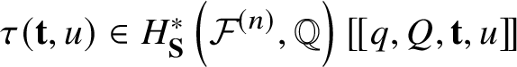

such that the following are true:
1.
$\tau ({\textbf t},u) = {\textbf t} + \pi ^*u +O(q,Q)$.2.
$P({\textbf t},u, z) = 1 +O(q,Q)$.3.
$ G ({\textbf t})- S^*_{\tau \left ({\textbf t},u\right )} (z) (P(\tau ({\textbf t},u),z)) \in z^{-2}H^*_{\textbf S}\left ({\mathcal {F}}^{(n)}, {\mathbb Q}\right )\left [\!\left [z^{-1},q, Q, {\textbf t}, u\right ]\!\right ] $ using the $z^{-1}$-expansion at simple poles.


Proof. We first write
 $$ \begin{align*}P : = \sum_{\left(d,D\right)} q^dQ^D P_{\left(d, D\right)} \quad \mathrm{and} \quad \tau : = \sum_{\left(d,D\right)} q^dQ^D \tau_{\left(d, D\right)} \end{align*} $$
and find  $P_{\left (d, D\right )}$ and $\tau _{\left (d, D\right )}$ inductively. We will use an induction on the partial order
 $$ \begin{align*}(d',D') < (d,D) \iff D'<D \quad \mathrm{or} \quad D'=D, \ d'<d. \end{align*} $$
For  $(d,D)=0$, we set $P_0: =1$ and $\tau _0({\textbf t}, u) :={\textbf t} + \pi ^*u$ so that they satisfy 1 and 2. For the coefficient of $q^0Q^0$, 3 follows from the asymptotic property
 $$ \begin{align} S^*_{{\textbf{t}}+\pi^*u}(z)(\gamma) = e^{\left({\textbf{t}} +\pi^*u\right)/z} \gamma\rvert_{q=0} + O(q) \end{align} $$
and the initial condition for G.
Now we fix  $(d,D)$. Suppose that $P_{\left (d',D'\right )}$ and $\tau _{\left (d',D'\right )}$ are determined for all $(d',D')<(d,D)$ such that after $z^{-1}$-expansion, the equality
 $$ \begin{align} G = S^*_{\tau} (P(\tau)) \mod z^{-2} \end{align} $$
holds in all coefficients of  $q^{d'}Q^{D'}$ with $(d',D') < (d,D)$. By comparing the coefficients of $q^dQ^D$ in both sides of this equation, we can uniquely determine $P_{\left (d,D\right )}$ and $\tau _{\left (d,D\right )}$ as follows. Using the asymptotic property (2.4.16), we write the right-hand side of equation (2.4.17) as
 $$ \begin{align*}S^*_{\tau}(P(\tau))\ =\ e^{\frac{\tau\left( {\textbf t }, u\right)}{z}}P(\tau) +O(q,Q). \end{align*} $$
The coefficient of  $q^dQ^D$ in $O(q,Q) \mod z^{-2}$ is already determined by the induction assumption. The coefficient of $q^dQ^D$ in $e^{\frac {\tau \left ({\textbf t}, u\right )}{z}}P(\tau )$ is
 $$ \begin{align*}e^{\frac{\textbf{t} + \pi^*u }{z}} \left( P_{\left(d,D\right)}+ \frac{1}{z}\tau_{\left(d,D\right)} \right) + \left(\left(\text{mod } z^{-2}\right)-\text{known terms by the induction}\right). \end{align*} $$
So  $P_{\left (d,D\right )}+ \frac {1}{z}\tau _{\left (d,D\right )}$ is uniquely determined up to mod $z^{-2}$. It determines $P_{\left (d,D\right )}$ and $\tau _{\left (d,D\right )}$.
By Proposition 2,  $S^*_{\tau } (P(\tau ))$ satisfies the characterisation properties. Now we would like to prove Theorem 3. We assume G satisfies the properties as well. Set $F^{\mu } := \mu ^* S^*_{\tau } (P(\tau ))$. Lemma 1 implies that $G^{\mu } = F^{\mu } \mod z^{-2}$, after $z^{-1}$-expansion, for all $\mu $. The next lemma tells us that they are actually equal as rational functions. It follows from the idea in [Reference Ciocan-Fontanine and Kim6, Lemma 7.7.1].
Lemma 2. We obtain  $G^{\mu } = F^{\mu }$ as rational functions for all $\mu $.
Proof. We first write
 $$ \begin{align*}G^{\mu} := \sum_{\left({\textbf l}=\left(l_i\right),{\textbf m}=\left(m_j\right),d,D\right)} q^d Q^D \prod_i t_i^{l_i} \prod_j u_j^{m_j} \cdot G^{\mu}_{\left({\textbf l}=\left(l_i\right),{\textbf m}=\left(m_j\right),d,D\right)}.\end{align*} $$
Let  $F^{\mu }_{\left ({\textbf l},{\textbf m},d,D\right )}$ be a function similarly defined using $F^{\mu }$. For the proof, we will use an induction on $({\textbf l},{\textbf m},d,D)$ for the colexicographic order,
 $$ \begin{gather*} ({\textbf l}',{\textbf m}',d',D') < ({\textbf l},{\textbf m},d,D) \\ \iff D' < D, \text{ or } D'=D, \ d' < d, \text{ or } D'=D, \ d'=d, \ {\textbf m}' < {\textbf m}, \\ \text{or } D'=D, \ d'=d, \ {\textbf m}' = {\textbf m}, \ {\textbf l}'<{\textbf l}. \end{gather*} $$
We would like to recall  ${\textbf l} \in {\mathbb Z}_{\geq 0}^{n}$, ${\textbf m} \in {\mathbb Z}_{\geq 0}^{\left \lvert {\mathrm {rank}} H^*(Y)\right \rvert }$, $d \in {\mathbb Z}^n$ and $D \in \mathrm {Eff}(Y)$. As the first step of the induction, we have $G^{\mu }_{\left ({\textbf l},{\textbf m},0,0\right )} = F^{\mu }_{\left ({\textbf l},{\textbf m},0,0\right )}$ for all ${\textbf l}$ and ${\textbf m}$, since both $G^{\mu }$ and $F^{\mu }$ follow the initial condition.
Now we fix  $({\textbf l},{\textbf m},d,D)$ with $(d,D) \neq (0,0)$. Suppose that
 $$ \begin{align*}G^{\mu}_{\left({\textbf l}',{\textbf m}',d',D'\right)} = F^{\mu}_{\left({\textbf l}',{\textbf m}',d',D'\right)}\end{align*} $$
for all  $({\textbf l}',{\textbf m}',d',D') < ({\textbf l},{\textbf m},d,D)$ and for all $\mu $. We will show that
 $$ \begin{align} G_{\left({\textbf l},{\textbf m},d,D\right)}^{\mu} = F_{\left({\textbf l},{\textbf m},d,D\right)}^{\mu} \end{align} $$
in several steps.
Step 1. For any  ${\textbf l}'$ and ${\textbf m}'$, we have
 $$ \begin{align} G_{\left({\textbf l}',{\textbf m}',d,D\right)}^{\mu}-F_{\left({\textbf l}',{\textbf m}',d,D\right)}^{\mu} \in H^*_{\textbf S} (Y, {\mathbb Q})\left[z, z^{-1}\right] \end{align} $$
for all  $\mu $ as rational functions in z. Here is a proof. Since
 $$ \begin{align*}\left({\textbf l}',{\textbf m}',d-kd_{\mu,\nu},D\right) < ({\textbf l},{\textbf m},d,D) \end{align*} $$
for any  $k>0$ and $\nu $, we have
 $$ \begin{align} \mathrm{Res}_{z=-\frac{\chi_{\mu,\nu}}{k}} G^{\mu}_{\left({\textbf l}',{\textbf m}',d,D\right)}(z) dkz & = \frac{q^{kd_{\mu,\nu}}}{e_{\textbf{S}}\left(N^{vir}_{\mu,\nu,k}\right)} \mu^* \mu_* G^{\nu}_{\left({\textbf l}',{\textbf m}',d-kd_{\mu,\nu},D\right)} \left(-\frac{\chi_{\mu, \nu}}{k}\right) \nonumber \\ & =\frac{q^{kd_{\mu,\nu}}}{e_{\textbf{S}}\left(N^{vir}_{\mu,\nu,k}\right)} \mu^* \mu_* F^{\nu}_{\left({\textbf l}',{\textbf m}',d-kd_{\mu,\nu},D\right)} \left(-\frac{\chi_{\mu, \nu}}{k}\right) \nonumber \\ & = \mathrm{Res}_{z=-\frac{\chi_{\mu,\nu}}{k}} F^{\mu}_{\left({\textbf l}',{\textbf m}',d,D\right)}(z) dkz, \end{align} $$
where the first and third equalities follow from the recursion relation for  $G^{\mu }$ and $F^{\mu }$, respectively, and the second equality comes from the induction assumption. Then formula (2.4.19) is obtained by the pole conditions in the recursion relation and equation (2.4.20).
Step 2. By formula (2.4.19) and Lemma 1, we obtain
 $$ \begin{align} G_{\left({\textbf l}',{\textbf m}',d,D\right)}^{\mu}-F_{\left({\textbf l}',{\textbf m}',d,D\right)}^{\mu} \in z^{-2}H^*_{\textbf S} (Y, {\mathbb Q})\left[z^{-1}\right] \end{align} $$
for any  ${\textbf l}'$, ${\textbf m}'$ and $\mu $.
Step 3. Recall that  $\left \{ \delta _j \right \}$ is a basis for $H^*(Y, {\mathbb Q})$. Let $\left \{\delta ^j\right \}$ be its dual basis. We write $G^{\mu }_{\left ({\textbf l}, {\textbf m}, d, D\right )}$ as
 $$ \begin{align*} G^{\mu}_{\left({\textbf l}, {\textbf m}, d, D\right)} = \sum_{ j} G^{\mu,j}_{\left({\textbf l},{\textbf m},d,D\right)} \delta^j \end{align*} $$
and consider the similar expression for  $F^{\mu }_{\left ({\textbf l}, {\textbf m}, d, D\right )}$. Let $\Delta ^{\mu , j}$ be the difference
 $$ \begin{align*} \left(z\partial_{u_j} G^{\mu}(z,q) , G^{\mu}\left(-z, qe^{-z\sum_i y_i E_{i,\mu} } \right)\right)_Y - \left(z\partial_{u_j} F^{\mu}(z,q) , F^{\mu}\left(-z, qe^{-z\sum_i y_i E_{i,\mu} } \right)\right)_Y, \end{align*} $$
let  $\Delta ^{\mu , j}_{\left ({\textbf l},{\textbf m},d,D\right )}$ be the coefficient of degree the $({\textbf l},{\textbf m},d,D)$-term in $\Delta ^{\mu , j}$ and let ${\textbf e}_j:=(0,\ldots ,0,1,0,\ldots , 0) \in {\mathbb Z}_{\geq 0}^{\left \lvert {\mathrm {rank}} H^*(Y)\right \rvert }$ be the jth standard basis. Then by the induction assumption, we can check that
 $$ \begin{align} \Delta^{\mu,j}_{\left({\textbf l},{\textbf m},d,D\right)} ={} & z\left(m_j +1\right) \left(G_{\left({\textbf l},{\textbf m}+ {\textbf e}_j,d,D\right)}^{\mu,0}-F_{\left({\textbf l},{\textbf m}+{\textbf e}_j,d,D\right)}^{\mu,0}\right) \\ & -\left(m_j +1\right)\sum_{j' \neq j} \left(G_{\left({\textbf l},{\textbf m}+ {\textbf e}_j-{\textbf e}_{j'},d,D\right)}^{\mu,j'}-F_{\left({\textbf l},{\textbf m}+{\textbf e}_j- {\textbf e}_{j'},d,D\right)}^{\mu, j'}\right) \nonumber \\ & -m_j \left(G_{\left({\textbf l},{\textbf m},d,D\right)}^{\mu, j}-F_{\left({\textbf l},{\textbf m},d,D\right)}^{\mu, j}\right) \nonumber \\ & +e^{-z\sum_i y_i \left(d_i - \left(d_{D,\mu}\right)_i \right)} \left(G_{\left({\textbf l},{\textbf m},d,D\right)}^{\mu, j}(-z)-F_{\left({\textbf l},{\textbf m},d,D\right)}^{\mu, j}(-z)\right).\nonumber \end{align} $$
By formula (2.4.21), we may write
 $$ \begin{align} G_{\left({\textbf l},{\textbf m},d,D\right)}^{\mu, j}-F_{\left({\textbf l},{\textbf m},d,D\right)}^{\mu, j} = z^{-2}\left(A^{j,{\textbf l},{\textbf m}}_0 +\frac{A^{j,{\textbf l},{\textbf m}}_1}{z} + \cdots \right), \end{align} $$
where  $A^{j,{\textbf l},{\textbf m}}_0,A^{j,{\textbf l},{\textbf m}}_1, \ldots \in {\mathbb Q}(\lambda )$ are uniquely determined $\lambda $-functions. Putting equation (2.4.23) into equation (2.4.22), we observe that the coefficient of $z^{-1}$ is
 $$ \begin{align} \sum_{s>0} \frac{1}{s!} A^{j,{\textbf l},{\textbf m}}_{s-1} \left(\sum_i y_i \left( d_i - \left(d_{D,\mu}\right)_i \right) \right)^{s} + A^{0,{\textbf l}, {\textbf m}+{\textbf e}_j}_0. \end{align} $$
The polynomiality condition for  $G^{\mu }$ and $F^{\mu }$ says that this coefficient must be zero for every j. Hence we have $A^{j,{\textbf l},{\textbf m}}_s=0$ for all s when $d \neq d_{D, \mu }$.
Step 4. When  $d = d_{D, \mu }$, equation (2.4.18) follows from the initial condition for both G and F. Since both $G^{\mu }_Y(-z)$ and $F^{\mu }_Y(-z)$ lie on $-z^{-1}{\mathcal {L}}^{\mu }_Y$, and they are equal to each other up to $z^{-2}H^*_{\textbf S} (Y, {\mathbb Q})\left [z^{-1}\right ] \otimes _{\mathbb Q} {\mathbb Q}[\![Q, {\textbf t}, u]\!]$, we have $G^{\mu }_Y(-z)=F^{\mu }_Y(-z)$ by the reconstruction of ${\mathcal {L}}^{\mu }_Y$ [Reference Coates and Givental8, Proposition 1, or Section 8].

3. Recursion relation for I-function
In this section, we would like to prove the following proposition:
Proposition 3. For each fixed locus  $\mu $, $I^{{\textbf {S}},\mu }_{{\mathcal {F}}^{(n)}}:=\mu ^*I^{\textbf S}_{{\mathcal {F}}^{(n)}} $ has simple poles at $z=-\chi _{\mu , \nu }/k$ for $k \in {\mathbb N}$, with residues
 $$ \begin{align} \mathrm{Res}_{z=-\frac{\chi_{\mu,\nu}}{k}} I^{{\textbf{S}},\mu}_{{\mathcal{F}}^{(n)}}(z) dkz = \frac{q^{kd_{\mu,\nu}}}{e_{\textbf{S}}\left(N^{vir}_{\mu,\nu,k}\right)} e_{\textbf{S}}\left(N_{Y^{\mu} / {\mathcal{F}}^{(n)}}\right) I^{{\textbf{S}},\nu}_{{\mathcal{F}}^{(n)}} \left(-\frac{\chi_{\mu, \nu}}{k}\right). \end{align} $$
Note that this proposition does not guarantee that these are all simple poles.
Before providing a proof, we introduce some terminology in combinatorics. Each fixed locus  $\mu : Y \rightarrow {{\mathcal {F}}^{(n)}}$ is assigned to $I^{\mu } = \left (I^{\mu }_0, I^{\mu }_1, \ldots , I^{\mu }_{n}, I^{\mu }_{n+1}\right )$, an ascending chain of subsets of $[r] := \{1,2,\ldots ,r\}$:
 $$ \begin{align*}\emptyset =: I^{\mu}_0 \subset I_1^{\mu} \subset I^{\mu} _2 \subset \cdots \subset I^{\mu}_n \subset I^{\mu}_{n+1} := [r], \qquad \left\lvert I^{\mu} _i\right\rvert = r_i.\end{align*} $$
Two different fixed loci  $\mu $ and $\nu $ are connected by a $1$-dimensional orbit if there are integers $\alpha _{\mu ,\nu }, \beta _{\mu ,\nu } \in [r]$ such that $I^{\mu }$ is replaced with $I^{\nu }$ by exchanging $\alpha _{\mu ,\nu }$ and $\beta _{\mu , \nu }$. Let $n^0_{\mu ,\nu } and n^1_{\mu ,\nu }$, $0 \leq n^0_{\mu ,\nu } \leq n^1_{\mu ,\nu } \leq n$, be indices determined by
 $$ \begin{align*} n^0_{\mu,\nu} & := \max \left\{i : \left\lvert I^{\mu}_i \cap \left\{\alpha_{\mu,\nu} , \beta_{\mu,\nu}\right\} \right\rvert = 0 \right\}, \\ n^1_{\mu,\nu} & := \max \left\{i : \left\lvert I^{\mu}_i \cap \left\{\alpha_{\mu,\nu} , \beta_{\mu,\nu}\right\} \right\rvert = 1 \right\}. \end{align*} $$
Since  $\mu \neq \nu $, we have $n^0_{\mu ,\nu } < n^1_{\mu ,\nu }$. We distinguish $\alpha _{\mu ,\nu }$ and $\beta _{\mu ,\nu }$ by the property
 $$ \begin{align} \alpha_{\mu,\nu} \in I^{\mu}_{n^1_{\mu,\nu}},\qquad \beta_{\mu,\nu} \notin I^{\mu}_{n^1_{\mu,\nu}} \end{align} $$
(hence  $\alpha _{\mu ,\nu }= \beta _{\nu ,\mu }$).
The family of  $1$-dimensional orbits connecting $Y^{\mu }$ to $Y^{\nu }$ is isomorphic to ${\mathbb P}\left (L_{\alpha _{\mu ,\nu }} \oplus L_{\beta _{\mu ,\nu }}\right ) \subset {\mathcal {F}}^{(n)}$. Note that the convention (3.0.26) is equivalent to
 $$ \begin{align*}Y^{\mu} \cong {\mathbb P}\left(L_{\alpha_{\mu,\nu}} \oplus 0 \right), \qquad Y^{\nu} \cong {\mathbb P}\left( 0 \oplus L_{\beta_{\mu,\nu}} \right).\end{align*} $$
On the corresponding component  $Y \hookrightarrow \overline {{\mathcal {M}}}_{0,2}\left ({\mathcal {F}}^{(n)}, kd_{\mu ,\nu }\right )^{\textbf {S}}$, the universal curve is also isomorphic to ${\mathbb P}\left (L_{\alpha _{\mu ,\nu }} \oplus L_{\beta _{\mu ,\nu }}\right )$, and the universal morphism from the universal curve ${\mathbb P}\left (L_{\alpha _{\mu ,\nu }} \oplus L_{\beta _{\mu ,\nu }}\right )$ to ${\mathbb P}\left (L_{\alpha _{\mu ,\nu }} \oplus L_{\beta _{\mu ,\nu }}\right ) \subset {\mathcal {F}}^{(n)}$ is the k-covering morphism. We denote it by $f_k$.
Proof of Proposition 3. We divide the proof into several steps.
Step 1. In the first step, we check that  $I^{{\textbf S},\mu }_{{\mathcal {F}}^{(n)}}$ has simple poles at $z=-\chi _{\mu ,\nu }/k$, $k=1,2,3,\ldots $.
The Atiyah–Bott localisation theorem tells us that for an equivariant class  $K \in H^2\left ({\mathbb P}\left (L_{\alpha _{\mu ,\nu }} \oplus L_{\beta _{\mu ,\nu }}\right ), {\mathbb Q}\right )$, we obtain
 $$ \begin{align} d_{\mu,\nu}(K) \cdot 1 = p_*(K) = \frac{\mu^*K - \nu^*K}{\chi_{\mu,\nu}} \in H^0(Y, {\mathbb Z}) \cong {\mathbb Z}, \end{align} $$
where  $p: {\mathbb P}\left (L_{\alpha _{\mu ,\nu }} \oplus L_{\beta _{\mu ,\nu }}\right ) \rightarrow Y$ is the projection morphism.
Recall that  $H_{n+1,j} = -c_1\left (\pi ^*L_j\right )$. For simplicity, we denote $H_j:= -c_1\left (\pi ^*L_j\right )$ during the proof. We obtain
 $$ \begin{align} 0 & = \mu^*H_{\alpha_{\mu,\nu}} - \nu^*H_{\alpha_{\mu,\nu}} = \mu^*H_{\beta_{\mu,\nu}} - \nu^*H_{\beta_{\mu,\nu}}, \\ \nonumber \chi_{\mu,\nu} & = \mu^*H_{\alpha_{\mu,\nu}} - \nu^*H_{\beta_{\mu,\nu}} = \nu^*H_{\alpha_{\mu,\nu}} - \mu^*H_{\beta_{\mu,\nu}}, \end{align} $$
by applying  $K=H_j$ and $\mathcal {S}^{\vee }$ the dual of the tautological bundle over ${\mathbb P}\left (L_{\alpha _{\mu ,\nu }} \oplus L_{\beta _{\mu ,\nu }}\right )$. Then by putting the equations (3.0.28) to $\mu ^*(\text {formula}$ (1.4.3)), we observe that $I^{{\textbf S},\mu }_{{\mathcal {F}}^{(n)}}$ has simple poles at $z=-\chi _{\mu ,\nu }/k$, $k=1,2,3,\ldots $.
Step 2. In the second step, we compute  $ \frac { e_{\textbf {S}}\left (N^{vir}_{\mu ,\nu ,k}\right ) }{e_{\textbf {S}}\left (N_{Y^{\mu } /{{\mathcal {F}}^{(n)}}}\right )}$ explicitly. From the definition of the virtual normal bundle $N^{vir}_{\mu ,\nu ,k}$ [Reference Graber and Pandharipande13], we have
 $$ \begin{align} e_{\textbf{S}}\left(N^{vir}_{\mu,\nu,k}\right) = \frac{e_{\textbf{S}}\left(R^0p_*\left(f^*_kT_{{{\mathcal{F}}^{(n)}}}\middle\rvert_{{\mathbb P}\left(L_{\alpha_{\mu,\nu}} \oplus L_{\beta_{\mu,\nu}}\right)}\right) ^{\mathrm{mov}} \right) }{e_{\textbf{S}}\left(R^1p_*\left(f^*_kT_{{{\mathcal{F}}^{(n)}}}\middle\rvert_{{\mathbb P}\left(L_{\alpha_{\mu,\nu}} \oplus L_{\beta_{\mu,\nu}}\right)}\right) ^{\mathrm{mov}} \right) } \cdot \frac{-\left(\mu^*H_{\beta_{\mu,\nu}} -\mu^*H_{\alpha_{\mu,\nu}}\right)^2}{e_{\textbf{S}}\left(R^0p_*\left( T_{p}\right)\right)}. \end{align} $$
The first fractional term on the right-hand side is obtained by deformation-obstruction spaces of the universal morphism, and the second fractional term on the right-hand side is obtained by automorphism spaces of the universal curve with two branch points. Here,  $T_p \cong \ker \left (T_{{\mathbb P}\left (L_{\alpha _{\mu ,\nu }} \oplus L_{\beta _{\mu ,\nu }}\right )} \rightarrow p^* T_Y\right )$ is the relative tangent bundle of p.
We can compute  $ \frac { e_{\textbf {S}}\left (N^{vir}_{\mu ,\nu ,k}\right ) }{e_{\textbf {S}}\left (N_{Y^{\mu } /{{\mathcal {F}}^{(n)}}}\right )}$ using equation (3.0.29). The restriction of the tangent bundle $T_{{\mathcal {F}}^{(n)}}$ to ${\mathbb P}\left (L_{\alpha _{\mu ,\nu }} \oplus L_{\beta _{\mu ,\nu }}\right )$ becomes
 $$ \begin{align}&T_Y \oplus \oplus_{i \leq n^0_{\mu,\nu}} {\mathrm{Hom}}\left( \oplus_{j \in I^{\mu}_{i-1}} L_j , \oplus_{j \in I^{\mu}_i \backslash I^{\mu}_{i-1}} L_j \right) \nonumber \\ &\oplus {\mathrm{Hom}}\left(\oplus _{j \in I^{\mu}_{r_{n^0_{\mu,\nu}}}} L_j , \oplus _{j \in I^{\mu}_{r_{n^0_{\mu,\nu}+1}} \backslash I^{\mu}_{r_{n^0_{\mu,\nu}} } , j \neq \alpha_{\mu,\nu}} L_j \oplus \mathcal{S} \right) \nonumber \\ &\oplus \oplus_{n^0_{\mu,\nu} +1 < i \leq n^1_{\mu,\nu}} {\mathrm{Hom}}\left(\oplus _{j \in I^{\mu}_{i } , j \neq \alpha_{\mu,\nu}} L_j \oplus \mathcal{S}, \oplus _{j \in I^{\mu}_{i+1} \backslash I^{\mu}_{i } } L_j \right) \nonumber \\ &\oplus {\mathrm{Hom}}\left(\oplus _{j \in I^{\mu}_{r_{n^1_{\mu,\nu}}}, j \neq \alpha_{\mu,\nu}} L_j \oplus \mathcal{S} , \oplus _{j \in I^{\mu}_{r_{n^1_{\mu,\nu}+1}} \backslash I^{\mu}_{r_{n^1_{\mu,\nu}} } , j \neq \beta_{\mu,\nu}} L_j \oplus \mathcal{S}^{\vee} \right) \nonumber \\ &\oplus \oplus_{i> n^1_{\mu,\nu}+1} {\mathrm{Hom}}\left( \oplus_{j \in I^{\mu}_{i-1}} L_j , \oplus_{j \in I^{\mu}_i \backslash I^{\mu}_{i-1}} L_j \right ). \end{align} $$
 In (3.0.30), all bundles over Y are considered to be pullbacks to  ${\mathbb P}\left (L_{\alpha _{\mu ,\nu }} \oplus L_{\beta _{\mu ,\nu }}\right )$ along the projection morphism p. Since the moving part occurs where $\mathcal {S}$ or $\mathcal {S}^{\vee }$ exists, we obtain
 $$ \begin{align} &\frac{e_{\textbf{S}}\left(R^0p_*\left(f^*_kT_{{{\mathcal{F}}^{(n)}}}\middle\rvert_{{\mathbb P}\left(L_{\alpha_{\mu,\nu}} \oplus L_{\beta_{\mu,\nu}}\right)}\right) ^{\mathrm{mov}} \right) }{e_{\textbf{S}}\left(R^1p_*\left(f^*_kT_{{{\mathcal{F}}^{(n)}}}\middle\rvert_{{\mathbb P}\left(L_{\alpha_{\mu,\nu}} \oplus L_{\beta_{\mu,\nu}}\right)}\right) ^{\mathrm{mov} }\right) } \nonumber\\ &\qquad\qquad\qquad\qquad = \prod_{ l \in I^{\mu}_{ n^0_{\mu,\nu}} } \left( \prod_{s=1}^{k -1}\left(\mu^* H_{l}-\mu^* H_{\alpha_{\mu,\nu}} + s\frac{\chi_{\mu, \nu}}{k}\right) \right)^{-1} \nonumber\\ &\quad\qquad\qquad\qquad\qquad \times \prod_{ l' \in \left( I^{\mu}_{ n^1_{\mu,\nu}+1} \backslash I^{\mu}_{n^0_{\mu,\nu} +1} \right) , l' \neq \beta_{\mu,\nu} } \left( \prod_{s=0}^{k }\left(\mu^* H_{\alpha_{\mu,\nu}}-\mu^* H_{l'}-s\frac{\chi_{\mu, \nu}}{k}\right) \right) \nonumber\\ &\quad\qquad\qquad\qquad\qquad\times \prod_{ l \in I^{\mu}_{ n^1_{\mu,\nu}} , l \neq \alpha_{\mu,\nu} } \left( \prod_{s=0}^{k }\left(\mu^* H_{l}-\mu^* H_{\beta_{\mu,\nu}}-s\frac{\chi_{\mu, \nu}}{k}\right) \right) \nonumber\\ &\quad\qquad\qquad\qquad\qquad \times \prod_{s=0}^{2k}\left(\mu^*H_{\alpha_{\mu,\nu}} -\mu^*H_{\beta_{\mu,\nu}} -s\frac{\chi_{\mu,\nu}}{k} \right). \end{align} $$
We also obtain
 $$ \begin{align} \frac{-\left(\mu^*H_{\beta_{\mu,\nu}} -\mu^*H_{\alpha_{\mu,\nu}}\right)^2}{e_{\textbf{S}}\left(R^0p_*\left( T_{p}\right)\right)} = \left(\mu^*H_{\alpha_{\mu,\nu}} -\mu^*H_{\beta_{\mu,\nu}} -\chi_{\mu,\nu} \right)^{-1} \end{align} $$
by a direct computation. Combining equations (3.0.28), (3.0.29), (3.0.31) and (3.0.32), we have
 $$ \begin{align} \frac{ e_{\textbf{S}}\left(N^{vir}_{\mu,\nu,k}\right) }{e_{\textbf{S}}\left(N_{Y^{\mu} /{{\mathcal{F}}^{(n)}}}\right)} & = \prod_{ l \in I^{\mu}_{ n^0_{\mu,\nu}} } \left( \prod_{s=0}^{k -1}\left(\mu^* H_{l} - \mu^* H_{\alpha_{\mu,\nu}} + s\frac{\chi_{\mu, \nu}}{k}\right) \right)^{-1} \\ & \quad \times \prod_{ l' \in \left( I^{\mu}_{ n^1_{\mu,\nu}+1} \backslash I^{\mu}_{n^0_{\mu,\nu} +1} \right) , l' \neq \beta_{\mu,\nu} } \left( \prod_{s=1}^{k }\left(\mu^* H_{\alpha_{\mu,\nu}}- \mu^* H_{l'}\ -\ s\frac{\chi_{\mu, \nu}}{k}\right) \right) \nonumber \\ & \quad \times \prod_{ l \in I^{\mu}_{ n^1_{\mu,\nu}} , l \neq \alpha_{\mu,\nu} } \left( \prod_{s=1}^{k }\left(\mu^* H_{l}\ -\ \mu^* H_{\beta_{\mu,\nu}}- s\frac{\chi_{\mu, \nu}}{k}\right) \right) \nonumber \\ & \quad \times \prod_{s=1}^{k-1}\left(\mu^*H_{\alpha_{\mu,\nu}} - \mu^*H_{\beta_{\mu,\nu}} - s\frac{\chi_{\mu,\nu}}{k} \right) \nonumber \\ & \quad \times \prod_{s=0}^{k-1}\left(\mu^*H_{\beta_{\mu,\nu}} -\ \mu^*H_{\alpha_{\mu,\nu}} + s\frac{\chi_{\mu,\nu}}{k} \right). \nonumber \end{align} $$
Using equation (3.0.28), one can see that this is equivalent to
 $$ \begin{align} \frac{ e_{\textbf{S}}\left(N^{vir}_{\mu,\nu,k}\right) }{e_{\textbf{S}}\left(N_{Y^{\mu} /{{\mathcal{F}}^{(n)}}}\right)} & = \prod_{ \ l \in I^{\nu}_{ n^0_{\mu,\nu}} } \left( \prod_{s=1}^{k }\left(\nu^* H_{l}-\nu^* H_{\beta_{\mu,\nu}} - s\frac{\chi_{\mu, \nu}}{k}\right) \right)^{-1} \\ \nonumber & \quad \times \prod_{ \ l' \in \left( I^{\nu}_{ n^1_{\mu,\nu}+1} \backslash I^{\nu}_{n^0_{\mu,\nu} +1} \right) , l' \neq \alpha_{\mu,\nu} } \left( \prod_{s=0}^{k -1}\left(\nu^* H_{\beta_{\mu,\nu}}-\nu^* H_{l'}+s\frac{\chi_{\mu, \nu}}{k}\right) \right) \\ & \quad \times \prod_{ \ l \in I^{\nu}_{ n^1_{\mu,\nu}} , l \neq \beta_{\mu,\nu} } \left( \prod_{s=0}^{k -1}\left(\nu^* H_{l}-\nu^* H_{\alpha_{\mu,\nu}} + s\frac{\chi_{\mu, \nu}}{k}\right) \right) \nonumber \\& \quad \times \prod_{\substack{s=0 \\s \neq k}}^{2k-1 }\left(\nu^*H_{\beta_{\mu,\nu}} -\nu^*H_{\alpha_{\mu,\nu}} +s\frac{\chi_{\mu,\nu}}{k} \right). \nonumber \end{align} $$
 Step 3. In the third step, we show that equation (3.0.25) holds true. From formula (1.4.3), we observe that each coefficient of  $I^{{\textbf S}, \mu }_{{\mathcal {F}}^{(n)}}(z)$ is
 $$ \begin{align} & \sum_{\sum_l d_i^l =d_i} \prod_{i=1}^n \left( \prod_{1 \leq l \neq l' \leq r_i}\frac{\prod_{s=-\infty}^{d_i^l -d_i^{l'}}\left(\mu^* H_{i,l}- \mu^* H_{i,l'}+sz\right) }{\prod_{s=-\infty}^{0}\left(\mu^*H_{i,l}-\mu^* H_{i,l'}+sz\right)} \right. \\ & \quad \times \left. \displaystyle \prod_{1 \leq l \leq r_i, 1 \leq l' \leq r_{i+1}}\frac{\prod_{s=-\infty}^{0}\left( \mu^* H_{i,l}-\mu^* H_{i+1,l'}+sz\right)}{\prod_{s=-\infty}^{d_i^l -d_{i+1}^{l'}}\left(\mu^* H_{i,l}-\mu^* H_{i+1,l'}+sz\right)} \right) \nonumber \\ & = \sum_{\sum_l d_i^l =d_i} \prod_{i=1}^n \left( \prod_{1 \leq l \neq l' \leq r_i}\frac{\prod_{s=-\infty}^{d_i^l -d_i^{l'}}\left(\mu^* H_{\sigma_{\mu}(l)}- \mu^* H_{\sigma_{\mu}(l')}+sz\right) }{\prod_{s=-\infty}^{0}\left(\mu^*H_{\sigma_{\mu}(l)}-\mu^* H_{\sigma_{\mu}(l')}+sz\right)} \right. \nonumber \\ & \quad \times \left. \displaystyle \prod_{1 \leq l \leq r_i, 1 \leq l' \leq r_{i+1}}\frac{\prod_{s=-\infty}^{0}\left( \mu^* H_{\sigma_{\mu}(l)}- \mu^* H_{\sigma_{\mu}(l')}+sz\right)}{\prod_{s=-\infty}^{d_i^l -d_{i+1}^{l'}}\left(\mu^* H_{\sigma_{\mu}(l)}- \mu^* H_{\sigma_{\mu}(l')}+sz\right)} \right),\nonumber \end{align} $$
where  $\sigma _{\mu }: [r] \rightarrow [r] \in \mathfrak {S}_r$ is a permutation of r such that $[r_{i+1}] \backslash [r_i]$ maps to $I^{\mu }_{i+1} \backslash I^{\mu }_i$, $i=1, \ldots , n$. Note that $\sigma _{\mu }$ can be taken as any such permutation, because of the symmetry of $d_i^l$ for each i. We compute a residue of equation (3.0.35) at $z=-\chi _{\mu ,\nu }/k$. It is enough to consider the case when the denominator of the right-hand side of equation (3.0.35) contains a factor $\left (\mu ^* H_{\alpha _{\mu ,\nu }} - \mu ^* H_{\beta _{\mu ,\nu }} + kz\right )$. Then the residue is
 $$ \begin{align} \left(\text{equation}\ (3.0.35) \cdot \left(\mu^* H_{\alpha_{\mu,\nu}} - \mu^* H_{\beta_{\mu,\nu}} + kz\right) \right) \big\rvert_{z=-\chi_{\mu,\nu} /k}. \end{align} $$
To verify equation (3.0.25), it is enough to show that formula (3.0.36) is equal to
 $$ \begin{align} &\frac{ e_{\textbf{S}}\left(N^{vir}_{\mu,\nu,k}\right) }{e_{\textbf{S}}\left(N_{Y^{\mu} /{{\mathcal{F}}^{(n)}}}\right)} \sum_{\sum_l d_i^l =d^{\prime}_i} \prod_{i=1}^n \left( \prod_{1 \leq l \neq l' \leq r_i} \frac{\prod_{s=-\infty}^{d_i^l -d_i^{l'}}\left(\nu^* H_{\sigma_{\nu}(l)} - \nu^* H_{\sigma_{\nu}(l')} - s\chi_{\mu,\nu}/k\right) }{\prod_{s=-\infty}^{0}\left(\nu^*H_{\sigma_{\nu}(l)} - \nu^* H_{\sigma_{\nu}(l')} - s\chi_{\mu,\nu}/k\right)} \right.\nonumber \\ &\qquad\qquad\qquad \times \left. \prod_{1 \leq l \leq r_i, 1 \leq l' \leq r_{i+1}} \frac{\prod_{s=-\infty}^{0}\left( \nu^* H_{\sigma_{\nu}(l)} - \nu^* H_{\sigma_{\nu}(l')} - s\chi_{\mu,\nu}/k\right)}{\prod_{s=-\infty}^{d_i^l -d_{i+1}^{l'}}\left(\nu^* H_{\sigma_{\nu}(l)} - \nu^* H_{\sigma_{\nu}(l')} - s\chi_{\mu,\nu}/k\right)} \right) , \end{align} $$
where
 $$ \begin{align*}d^{\prime}_i = \begin{cases} d_i - k & \text{if } n^0_{\mu,\nu}< i \leq n^1_{\mu,\nu} , \\ d_i & \text{if } i \leq n^0_{\mu,\nu} \text{ or } n^1_{\mu,\nu} < i, \end{cases} \end{align*} $$
and  $\sigma _{\nu } =\sigma _{\mu } \circ \left (\alpha _{\mu ,\nu }, \beta _{\mu ,\nu }\right ) \in \mathfrak {S}_r$ is a permutation of $[r]$, because
 $$ \begin{align*} & \sum_{\sum_l d_i^l =d^{\prime}_i} \prod_{i=1}^n \left( \prod_{1 \leq l \neq l' \leq r_i}\frac{\prod_{s=-\infty}^{d_i^l -d_i^{l'}}\left(\nu^* H_{\sigma_{\nu}(l)}- \nu^* H_{\sigma_{\nu}(l')}-s\chi_{\mu,\nu}/k\right) }{\prod_{s=-\infty}^{0}\left(\nu^*H_{\sigma_{\nu}(l)}-\nu^* H_{\sigma_{\nu}(l')}-s\chi_{\mu,\nu}/k\right)} \right. \\ &\qquad\qquad\qquad\qquad\qquad\qquad \times\left. \prod_{1 \leq l \leq r_i, 1 \leq l' \leq r_{i+1}}\frac{\prod_{s=-\infty}^{0}\left( \nu^* H_{\sigma_{\nu}(l)}- \nu^* H_{\sigma_{\nu}(l')}-s\chi_{\mu,\nu}/k\right)}{\prod_{s=-\infty}^{d_i^l -d_{i+1}^{l'}}\left(\nu^* H_{\sigma_{\nu}(l)}- \nu^* H_{\sigma_{\nu}(l')}-s\chi_{\mu,\nu}/k\right)} \right) \end{align*} $$
is the coefficient of  $I^{{\textbf S}, \nu }_{{\mathcal {F}}^{(n)}}\left (-\chi _{\mu ,\nu }/k\right )$ and we have an identity
 $$ \begin{align*} e^{-\frac{\mu^*{\textbf{t}}}{ \chi_{\mu,\nu} / k}} q^d e^{\sum_i t_i d_i} = q^{kd_{\mu,\nu}} e^{-\frac{\nu^*{\textbf{t}}}{ \chi_{\mu,\nu} / k}} q^{d'} e^{\sum_i t_i d^{\prime}_i} \end{align*} $$
induced by equation (3.0.27) and
 $$ \begin{align*} d_{\mu,\nu}\left(\det {\mathcal{F}}_i^{\vee}\right) = \begin{cases} 1 & \text{if } n^0_{\mu,\nu}< i \leq n^1_{\mu,\nu}, \\ 0 & \text{if } i \leq n^0_{\mu,\nu} \text{ or } n^1_{\mu,\nu} < i. \end{cases} \end{align*} $$
Here,  $\left (\alpha _{\mu ,\nu }, \beta _{\mu ,\nu }\right )$ denotes the permutation exchanging $\alpha _{\mu ,\nu }$ and $\beta _{\mu ,\nu }$. For any integers m and $l \neq \alpha _{\mu ,\nu }, \beta _{\mu ,\nu }$, we obtain
 $$ \begin{align} & \frac{\prod_{s=-\infty}^{m}\left( \mu^* H_{\alpha_{\mu,\nu}}- \mu^* H_{l} - s\chi_{\mu,\nu} / k\right)}{\prod_{s=-\infty}^{0}\left(\mu^* H_{\alpha_{\mu,\nu}}- \mu^* H_{l} - s\chi_{\mu,\nu} / k\right)} \\ \nonumber & = \frac{\prod_{s=-\infty}^{m}\left( \nu^* H_{\beta_{\mu,\nu}} + \chi_{\mu,\nu} - \nu^* H_{l} - s\chi_{\mu,\nu} / k\right)}{\prod_{s=-\infty}^{0}\left(\nu^* H_{\beta_{\mu,\nu}} +\chi_{\mu,\nu} - \nu^* H_{l} - s\chi_{\mu,\nu} / k\right)} \\ \nonumber & = \frac{\prod_{s=-\infty}^{m-k}\left( \nu^* H_{\beta_{\mu,\nu}}- \nu^* H_{l} - s\chi_{\mu,\nu} / k\right)}{\prod_{s=-\infty}^{0}\left(\nu^* H_{\beta_{\mu,\nu}}- \nu^* H_{l} - s\chi_{\mu,\nu} / k\right)} \prod_{s=0}^{k -1}\left(\nu^* H_{\beta_{\mu,\nu}}-\nu^* H_{l} + s\frac{\chi_{\mu, \nu}}{k}\right ), \end{align} $$
where the first equality comes from equation (3.0.28). Doing the same computations for  $l=\beta _{\mu ,\nu }$ and for the inverse of most of the left-hand side of equation (3.0.38)), putting all into equation (3.0.35) and using equation (3.0.34), we obtain that $\text {formula }$(3.0.36) $= \text {formula }$(3.0.37).
4. Quasimaps to GIT fibre bundles
In [Reference Ciocan-Fontanine, Kim and Maulik7], the quasimap moduli spaces  $Q_{g,k}(X, \beta )$ for a GIT quotient $X = W /\!\!/ \textbf {G}$ are constructed, which provide another compactification of ${\mathcal {M}}_{g,k}(X, \beta )$ (definition (1.1.1)). In [Reference Ciocan-Fontanine and Kim5, Reference Ciocan-Fontanine and Kim6], Ciocan-Fontanine and Kim showed that a certain generating function of invariants of ‘graph’ quasimap spaces lies on ${\mathcal {L}} ag_X$ and is equal to Givental’s I-function when X is a (complete intersection in) toric variety or partial flag variety [Reference Bertram, Ciocan-Fontanine and Kim2, Reference Ciocan-Fontanine and Kim5]. In this section, we will construct quasimap spaces for GIT fibre bundles. In Section 5 we will show that $I^{\textbf {S}}_{{\mathcal {F}}^{(n)}}$ can be written in terms of ‘graph’ quasimap spaces. Using this, we will show that it satisfies the characterisation properties so that we can conclude that $I^{\textbf S}_{{\mathcal {F}}^{(n)}}$ lies on the cone by Theorem 3.
4.1. GIT quotients and their presentations
Let  $\textbf {G}$ be a linearly reductive algebraic group acting on an affine variety V. Suppose that V has at worst locally complete intersection singularities. Let Y be a smooth projective variety and $\pi : E \rightarrow Y$ be a fibre bundle with the fibre V. Suppose there exists a fibrewise $\textbf {G}$-action satisfying the following property. For each $y \in Y$, there is an affine neighbourhood $U \subset Y$ and a $\textbf {G}$-equivariant isomorphism
 $$ \begin{align*}\varphi :\pi^{-1}(U) := E \times_Y U \rightarrow V \times U \end{align*} $$
such that  $p_2 \circ \varphi = \pi \rvert _{\pi ^{-1}(U)}$, where $p_2:V \times U \rightarrow U$ is the projection morphism.
For a fixed character  $\theta \in \chi (\textbf {G}):= {\mathrm {Hom}}({\textbf G}, {\mathbb C}^*)$, we define a GIT quotient
 $$ \begin{align*}E /\!\!/_{\theta}\textbf{G} := {\mathrm{Proj}} \bigoplus^{\infty}_{n=0}\left(R^0 \pi_{*}(E \times {\mathbb C}_{\theta})^{\otimes n}\right)^{\textbf{G}},\end{align*} $$
where  $\mathbb {C}_{\theta }$ is the $1$-dimensional representation of $\textbf {G}$ determined by $\theta $. Then $E /\!\!/_{\theta } \textbf {G}$ is a fibre bundle over Y with the fibre $V /\!\!/_{\theta } \textbf {G}$.
Suppose that for some  $r \in \mathbb {Z}_{>0}$ and $n_1, \ldots , n_r \in \mathbb {Z}_{>0}$, a $\textbf {T} :=(\mathbb {C}^*)^r$-action on V which commutes with the $\textbf {G}$-action on V, and a positive integer $m \in \mathbb {Z}_{>0}$, there is a morphism of varieties $\psi : Y \rightarrow \prod _{j=1}^r \mathbb {P}^{n_j -1}$,
 $$ \begin{align} \left(\psi: Y \rightarrow \prod_{j=1}^r \mathbb{P}^{n_j -1}, \ ({\textbf{T}} \times {\textbf{G}})\text{-action on } V, \ m \in \mathbb{Z}_{> 0}\right), \end{align} $$
which satisfies the following five conditions:
1. E is the pullback of a vector bundle
$\left [\left (\prod _{j=1}^r \mathbb {C}^{n_j}\right ) \times V / \textbf {T}\right ]$ on $\left [\left (\prod _{j=1}^r \mathbb {C}^{n_j}\right ) / \textbf {T}\right ]$ under the composition morphism between stacks: In other words, we have a fibre product$$ \begin{align*}Y \stackrel{\psi}{\longrightarrow} \prod_{j=1}^r \mathbb{P}^{n_j -1} \hookrightarrow \prod_{j=1}^r\left[\mathbb{C}^{n_j} / \mathbb{C}^*\right] \cong \left[ \left(\prod_{j=1}^r \mathbb{C}^{n_j}\right) / \textbf{T}\right]. \end{align*} $$(4.1.40)To simplify notation, we set$W:= \prod _{j=1}^r \mathbb {C}^{n_j}$ and $\widetilde {V} := W \times V$.2. The morphism
$E \rightarrow \left [\widetilde {V} / \textbf {T}\right ]$ in diagram (4.1.40) is $\textbf {G}$-equivariant.3.
$\Gamma \left ({\mathcal {O}}_{\widetilde {V}}\right )^{\textbf {T} \times \textbf {G}} \cong \mathbb {C}$ as $\mathbb {C}$-algebras.4.
$V^s(\textbf {G}, \theta )=V^{ss}(\textbf {G}, \theta ) \neq \emptyset $, and it is nonsingular. Moreover, the $\textbf {G}$-action on $V^s(\textbf {G}, \theta )$ is free.


Before stating the fifth condition, recall that  $\prod _{j=1}^r \mathbb {P}^{n_j -1} \cong W /\!\!/_{\textbf 1} \textbf {T}$, where ${\textbf 1} = (1, \ldots , 1) \in \chi (\textbf {T}) \cong {\mathbb Z}^r$. Set $\widetilde {\theta }:=m{\textbf 1} + \theta \in \chi (\textbf {T})\oplus \chi (\textbf {G}) \cong \chi (\textbf {T}\times \textbf {G})$. The fifth condition is then:
5.
$$ \begin{align*}\widetilde{V}^{ss}\left(\textbf{T} \times \textbf{G}, \widetilde{\theta}\right) = W^{ss}(\textbf{T},{\textbf 1}) \times V^{ss}(\textbf{G}, \theta).\end{align*} $$

Condition 4 guarantees that  $E /\!\!/_{\theta } \textbf {G}$ is nonsingular and an open substack of $[E/\textbf {G}]$. We write simply $E /\!\!/ \textbf {G}$ instead of $E /\!\!/_{\theta } \textbf {G}$. We will label both $E /\!\!/ \textbf {G} \rightarrow Y$ and $[E/\textbf {G}] \rightarrow Y$ by $\pi $ when the context is clear:

From conditions 1 and 2, we have a fibre diagram

Conditions 3 and 5 guarantee that the GIT quotient
 $$ \begin{align*}\widetilde{V} /\!\!/_{\widetilde{\theta}} (\textbf{T} \times \textbf{G}) \cong \left[\widetilde{V}^{ss}\left(\textbf{T} \times \textbf{G}, \widetilde{\theta}\right) / \textbf{T} \times \textbf{G}\right] \end{align*} $$
is a nonsingular, projective, open substack of  $\left [\widetilde {V}/\textbf {T} \times \textbf {G}\right ]$. Moreover,

is a fibre diagram, and hence  $E /\!\!/ \textbf {G}$ is projective as well.
Definition 1. A presentation of  $(E, {\textbf {G}}, \theta )$ is a datum (4.1.39) satisfying conditions 1–5.
4.2. Presentation of ${{\mathcal {F}}^{(n)}}$

Recall that  $L_j \rightarrow Y$, $j=1, \ldots , r$, are line bundles on Y, and $F:=\bigoplus _{j=1}^r L_j \rightarrow Y$ is the sum of $L_j$. We define
 $$ \begin{align*}E := \bigoplus_{i=1}^{n-1} \mathrm{Hom}\left(\mathcal{O}_Y^{\oplus r_i}, \mathcal{O}_Y^{\oplus r_{i+1}}\right) \oplus \mathrm{Hom}\left(\mathcal{O}_Y^{\oplus r_n}, F\right) \rightarrow Y \end{align*} $$
for given numbers  $0=r_0<r_1<\cdots <r_n<r_{n+1}=r$, where $\mathrm {Hom}(A,B)$ denotes the space ${\mathrm {Spec}}_{{\mathcal {O}}_Y} {\mathrm {Sym}} {\mathcal {H}} om_{{\mathcal {O}}_Y} (A,B)^{\vee }$. We define a $\textbf {G}:=\prod _{i=1}^n GL_{r_i}(\mathbb {C})$-action on E by
 $$ \begin{align*}E \times \textbf{G} \rightarrow E, \qquad \left((B_i)_{i=1}^n \in E, (A_i)_{i=1}^n \in {\textbf G}\right) \mapsto \left(A_{i+1}^{-1} \cdot B_i \cdot A_i\right)_{i=1}^n, \end{align*} $$
where  $A_{n+1} = \mathrm {Id}_r.$ Set $\theta :=\mathrm {det}^n \in \chi (\textbf {G})$. Then $V^s(\textbf {G}, \theta )=V^{ss}(\textbf {G}, \theta ) \neq \emptyset $, and it is nonsingular. Moreover, the $\textbf {G}$-action on $V^s(\textbf {G}, \theta )$ is free. The quotient $E /\!\!/ \textbf {G}$ is then isomorphic to ${{\mathcal {F}}^{(n)}}$.
Choose any ample line bundle  $\mathcal {O}(1)$ on Y and let
 $$ \begin{align*}E' := \bigoplus_{i=1}^{n-1} \mathrm{Hom}\left(\mathcal{O}_Y^{\oplus r_i}, \mathcal{O}_Y^{\oplus r_{i+1}}\right) \oplus \mathrm{Hom}\left(\mathcal{O}_Y^{\oplus r_n}, F(l)\right) \end{align*} $$
be a twisting of E for an integer  $l>0$. Then a $\textbf {G}$-action on $E'$ is defined in the same way as it acts on E.
Proposition 4. The quotients
 $$ \begin{align*}E' /\!\!/ {\textbf{G}} \cong E /\!\!/ \textbf{G} \end{align*} $$
are isomorphic as fibre bundles. Moreover  $(E', {\textbf {G}}, \theta )$ has a presentation (Definition 1) if l is large enough.
Proof. Take a positive integer l such that  $L_j' := L_j(l)$, $j=1, \ldots , r$, are generated by their global sections. Then $E /\!\!/_{\theta } \textbf {G} \cong E' /\!\!/_{\theta } \textbf {G}.$ Setting $n_j:=\mathrm {dim}H^0\left (Y,L_j'\right )$, we have a morphism
 $$ \begin{align*}\psi_j : Y \rightarrow \mathbb{P}\left(H^0\left(Y,L_j'\right)^{\vee}\right) \cong \mathbb{P}^{n_j -1}\end{align*} $$
such that  $\psi _j^*\left (\mathcal {O}_{\mathbb {P}^{n_j -1}}(1)\right ) \cong L_j'$, and therefore we obtain $\psi : Y \rightarrow \prod _{j=1}^r \mathbb {P}^{n_j -1}$. Define a $\textbf {T} := (\mathbb {C}^*)^r$-action on $V= \bigoplus _{i=1}^{n} \mathrm {Hom}\left (\mathbb {C}^{r_i}, \mathbb {C}^{r_{i+1}}\right )$ by
 $$ \begin{align*}\textbf{T} \times V \rightarrow V, \qquad \left((t_1, \ldots , t_r), (b_i)_{i=1}^n\right) \mapsto (b_1, \ldots, b_{n-1}, \mathrm{diag}(t_1, \ldots, t_r) \cdot b_n). \end{align*} $$
Conditions 1 and 2 for  $(E' , {\textbf {G}}, \theta )$ are satisfied with the $\psi $ and $\textbf {T} \times \textbf {G}$-action on V.
Consider the following  $\textbf {T} \times \mathbb {C}^*$-action on V:
 $$ \begin{align} V = \bigoplus_{i=1}^{n-1} \mathrm{Hom}\left(\mathbb{C}^{r_i}, \mathbb{C}^{r_{i+1}}\right) \oplus \mathrm{Hom}\left(\mathbb{C}^{r_n}, \bigoplus_{j=1}^r \mathbb{C}_{e_j + \mathrm{id}_{{\mathbb C}^*}}\right), \end{align} $$
where  $e_j$, $j=1,\ldots ,r$, are the standard basis for $\chi (\textbf {T}) \cong \mathbb {Z}^r$, and $\mathrm {id}_{\mathbb {C}^*} \in \chi (\mathbb {C}^*) $. Note that we consider the trivial action on ${\mathbb C}$ without a subscript. Set $u_j := e_j + \mathrm {id}_{{\mathbb C}^*} \in \chi (\textbf {T} \times \mathbb {C}^*)$ for each j. Set
 $$ \begin{align*}{\textbf 1} : = e_1 + \cdots + e_r \quad \text{and}\quad \alpha = \sum_{i=1}^n r_i \cdot \mathrm{id}_{{\mathbb C}^*} \in \chi(\textbf{T} \times \mathbb{C}^*). \end{align*} $$
Note that setting
 $$ \begin{align*}\lambda : \mathbb{C}^* \hookrightarrow \textbf{G}, \qquad t \mapsto \left(t \cdot \mathrm{Id}_{r_i}\right)_{i=1}^n,\end{align*} $$
we have  $\alpha = \theta \circ \lambda $. Now we can choose $m \in \mathbb {Z}_{>0}$ satisfying the following conditions:
•
$m{\textbf 1} + \alpha $ is in the interior of the cone generated by $e_1, \ldots , e_r, u_j$ for all $j=1, \ldots , r.$•
$m{\textbf 1} + \alpha $ is not in the cone generated by $e_1, \ldots , \hat {e_j}, \ldots , e_r, u_1, \ldots , u_r$ for all $j=1, \ldots , r.$


Then  $\left (\psi , ({\textbf {T}}\times {\textbf G}) \rightarrow \mathrm {Aut} (V), m \right )$ becomes a presentation of $(E', {\textbf {G}}, \theta )$.
4.3. Stable quasimaps
Suppose that  $(E,\textbf {G},\theta )$ has a presentation
 $$ \begin{align*}\left(\psi: Y\rightarrow \prod_{j=1}^r \mathbb{P}^{n_j -1} , \textbf{T} \times \textbf{G} \rightarrow \mathrm{Aut}(V) , m \in \mathbb{Z}_{>0}\right). \end{align*} $$
We choose a class
 $$ \begin{align} \beta = (\beta',\beta_0) \in \mathrm{Ker}\left( \mathrm{Pic}(Y)^{\vee} \oplus \mathrm{Pic}^{\textbf{T} \times \textbf{G}}(V)^{\vee} \rightarrow \chi(\textbf{T})^{\vee} \right), \end{align} $$
where the morphism is defined by using diagram (4.1.41). Here  $(-)^{\vee } = \mathrm {Hom}_{\mathbb {Z}}(-,{\mathbb Z})$. Note that for ${{\mathcal {F}}^{(n)}}$ (with the presentation in Section 4.2), choosing $\beta $ is equivalent to choosing a class in $H_2\left ({{\mathcal {F}}^{(n)}} , {\mathbb Z}\right )$. For $g,k \in \mathbb {Z}_{\geq 0}$ with $2g+k \geq 2$, consider the data
 $$ \begin{align} \left( \phi:(C,p_1, \ldots, p_k) \rightarrow (C_0,p_1,\ldots,p_k), f:C \rightarrow Y, P, u \right) \end{align} $$
satisfying the following conditions:
•
$(C,p_1, \ldots , p_k)$ and $(C_0,p_1, \ldots , p_k)$ are prestable k-pointed curves of genus g.•
$\phi $ is the contraction of all rational tails on C. A rational tail is a maximal (with respect to a partial order defined by inclusions) connected tree of rational curves with no marked points, attached to other components at only one node on C.• f is of degree
$\beta '$, and f restricted to each irreducible component of a rational tail is nonconstant.• P is a
$\textbf {G}$-principal bundle on $C_0$.•
$u \in \Gamma \left (C_0, P_f \times _{(\textbf {T} \times \textbf {G})} V \right )$.•
$\beta _0 (L)= \mathrm {deg}\left (u^*\left (P_f \times _{(\textbf {T} \times \textbf {G})} L\right )\right )$ for all $L \in \mathrm {Pic}^{\textbf {T} \times \textbf {G}}(V)$.


Here, the  $(\textbf {T} \times \textbf {G})$-principal bundle $P_f$ may be defined on $C_0$ by using f as follows [Reference Ciocan-Fontanine and Kim6]. For $1 \leq j_0 \leq r$, having
 $$ \begin{align*}C \stackrel{f}{\longrightarrow} Y \stackrel{\psi}{\longrightarrow} \prod_{j=1}^r \mathbb{P}^{n_j -1} \longrightarrow \mathbb{P}^{n_{j_0} -1} \end{align*} $$
is equivalent to the existence of a surjective morphism of sheaves on C
 $$ \begin{align*}\mathcal{O}_C^{\oplus n_{j_0}} \stackrel{\varphi_{j_0}}{\longrightarrow} \mathcal{L}_{j_0} \longrightarrow 0, \end{align*} $$
where  $\mathcal {L}_{j_0}$ is the pullback of $\mathcal {O}_{\mathbb {P}^{n_{j_0} -1}}(1)$ on C. Let $T_1 , \ldots , T_l$ be rational tails on C and $\widetilde {C} $ be the closure of $C \setminus \left (\cup _{i=1}^l T_i\right )$. Let $t_1 , \ldots , t_l$ be the corresponding points of $T_1, \ldots , T_l$ at $\widetilde {C}$. Consider the following morphism of sheaves on $\widetilde {C}$:
 $$ \begin{align*}\mathcal{O}_{\widetilde{C}}^{\oplus n_{j_0}} \xrightarrow{ \varphi_{j_0} \rvert_{\widetilde{C}}} \mathcal{L}_{j_0} \rvert_{\widetilde{C}} \longrightarrow \mathcal{L}_{j_0} \rvert_{\widetilde{C}} \otimes \mathcal{O}_{\widetilde{C}}\left(\sum_{i=1}^l \mathrm{deg}\left(\mathcal{L}_{j_0} \middle\rvert_{T_i}\right) \cdot t_i\right). \end{align*} $$
Since  $\widetilde {C}$ is isomorphic to $C_0$ through the composition $\widetilde {C} \hookrightarrow C \rightarrow C_0,$ this map gives rise to the morphism of stacks
 $$ \begin{align*}C_0 \rightarrow \left[\mathbb{C}^{n_{j_0}} / \mathbb{C}^*\right] \end{align*} $$
with degree  $\deg \mathcal {L}_{j_0}$. So we have the morphism of stacks
 $$ \begin{align*}C_0 \rightarrow \prod_{j=1}^r \left[\mathbb{C}^{n_j} / \mathbb{C}^*\right] \cong [W / \textbf{T}] \end{align*} $$
with degree  $d:=(\deg \mathcal {L}_1 , \ldots , \deg \mathcal {L}_r) \in \mathbb {Z}^r \cong \mathrm {Hom}\left (\mathrm {Pic}^{\textbf {T}}W, \mathbb {Z}\right )$. Note that d is the image of $\beta '$ under
 $$ \begin{align*}\mathrm{Pic}(Y)^{\vee} \rightarrow \mathrm{Pic}\left(\prod_{j=1}^r \mathbb{P}^{n_j -1}\right)^{\vee} \cong \mathrm{Pic}^{\textbf{T}}(W)^{\vee}.\end{align*} $$
In conclusion, we have the  $\textbf {T}$-principal bundle $Q_f$ on $C_0$, and the $\textbf {T}$-equivariant morphism
 $$ \begin{align} Q_f \rightarrow W. \end{align} $$
Now define  $P_f := Q_f \times _{C_0} P$.
We call the data (4.3.44) a genus g, k-pointed quasimap with degree  $\beta $, or simply a quasimap with type $(g,k,\beta )$. Now, we want to define a stability condition on quasimaps. For a quasimap with type $(g,k,\beta )$
 $$ \begin{align*}\left( \phi:(C,p_1, \ldots, p_k) \rightarrow (C_0,p_1,\ldots,p_k), f:C \rightarrow Y, P, u \right), \end{align*} $$
we have the morphism  $P_f \rightarrow W$ through formula (4.3.45), which defines the section $C_0 \rightarrow P_f \times _{(\textbf {T} \times \textbf {G})} W.$ Combining this with u, we have the section
 $$ \begin{align*}\widetilde{u} : C_0 \rightarrow P_f \times_{(\textbf{T} \times \textbf{G})} (W\times V).\end{align*} $$
Thus we obtain a quasimap  $\left (C_0, P_f, \widetilde {u}\right )$ in the sense of [Reference Ciocan-Fontanine, Kim and Maulik7].
Definition 2. A quasimap
 $$ \begin{align*}(\phi:(C,p_1, \ldots, p_k) \rightarrow (C_0,p_1,\ldots,p_k), f:C \rightarrow Y, P, u)\end{align*} $$
is  $\theta $ -prestable if $ \left (C_0, P_f, \widetilde {u}\right ) $ is $\left (\widetilde {\theta } = m{\textbf 1} + \theta \right )$-prestable in the sense of [Reference Ciocan-Fontanine, Kim and Maulik7]. It is $\theta $ -stable if, for each irreducible component $C' \subset C_0$, $f\rvert _{C'}$ is nonconstant or $\left (C_0, P_f, \widetilde {u}\right )\rvert _{C'}$ is $0^+$-stable in the sense of [Reference Ciocan-Fontanine, Kim and Maulik7] with respect to $\widetilde {\theta }$.
Definition 3. An isomorphism between two quasimaps
 $$ \begin{align*} \left( \phi:(C,p_1, \ldots, p_k) \rightarrow (C_0,p_1,\ldots,p_k), f:C \rightarrow Y, P, u \right) \text{ and} \\ \left( \phi':\left(C',p^{\prime}_1, \ldots, p^{\prime}_k\right) \rightarrow \left(C^{\prime}_0,p^{\prime}_1,\ldots,p^{\prime}_k\right), f':C' \rightarrow Y, P', u' \right) \end{align*} $$
is a tuple of isomorphisms
 $$ \begin{align*}\left( q:C \stackrel{ \sim }{\longrightarrow} C' , \xi : P \stackrel{ \sim }{\longrightarrow} q_0^*P' \right) \end{align*} $$
such that
 $$ \begin{align*}f' \circ q = f,\qquad q \circ p_a = p^{\prime}_a \qquad \text{and}\qquad q_0^* u' = (\zeta, \xi)\circ u, \end{align*} $$
where
•
$q_0: C_0 \stackrel {\sim }{\longrightarrow } C^{\prime }_0$ is an isomorphism between the contracted curves induced by q and•
$\zeta $ is an isomorphism $Q_f \stackrel {\sim }{\longrightarrow } q_0^*Q^{\prime }_{f'}$ between the $\textbf {T}$-principal bundles on $C_0$ induced by f and $f'$ which commutes the diagram


Note that  $\zeta $ is uniquely determined by the condition $f' \circ q = f$.
We denote the moduli space of (pre)stable quasimaps with type  $(g,k,\beta )$ by
 $$ \begin{align*}Q_{g,k}^{(pre)}(E /\!\!/ \textbf{G} ,\beta). \end{align*} $$
Then there is a morphism of moduli spaces of prestable quasimaps
 $$ \begin{align*}Q^{pre}_{g,k}(E /\!\!/ \textbf{G},\beta) \rightarrow Q^{pre}_{g,k} \left(\widetilde{V} /\!\!/_{\widetilde{\theta}} (\textbf{T} \times \textbf{G}) , \beta''\right),\end{align*} $$
where  $\beta '' := \deg \left (C_0,P_f,\widetilde {u}\right )$. The latter space is in the sense of [Reference Ciocan-Fontanine, Kim and Maulik7], which is an Artin stack, locally of finite type over $\mathbb {C}$. Since the stability condition is an open condition, $Q_{g,k}(E /\!\!/ \textbf {G},\beta )$ is an open substack of $Q^{pre}_{g,k}(E /\!\!/ \textbf {G},\beta )$.
4.4. Quasimap moduli spaces
Let  $\mathfrak {M}_{g,k}(Y,\beta ')$ be the stack of genus g, k-pointed prestable maps to Y with degree $\beta '$. It is an Artin stack, locally of finite type over $\mathbb {C}$. Let $\mathfrak {M}^{\prime }_{g,k}(Y,\beta ')$ be the substack of $\mathfrak {M}_{g,k}(Y,\beta ')$ whose objects are nonconstant on each component of a rational tail. $\mathfrak {M}^{\prime }_{g,k}(Y,\beta ')$ is an open substack of $\mathfrak {M}_{g,k}(Y,\beta ')$ [Reference Olsson15, Lemma 5.1]. There is a morphism of stacks
 $$ \begin{gather*} Q^{pre}_{g,k}(E /\!\!/ \textbf{G}, \beta) \rightarrow \mathfrak{M}^{\prime}_{g,k}(Y,\beta'), \\ \left( \phi:(C,p_1, \ldots, p_k) \rightarrow (C_0,p_1,\ldots,p_k), f , P, u \right) \mapsto \left((C,p_1, \ldots, p_k), f \right). \end{gather*} $$
We define a morphism of stacks
 $$ \begin{gather*} Q^{pre}_{g,k}\left(\widetilde{V} /\!\!/_{\widetilde{\theta}} (\textbf{T} \times \textbf{G}) , \beta'' \right) \rightarrow Q^{pre}_{g,k}\left(W /\!\!/_{\textbf 1} \textbf{T}, d\right), \\ \left((C_0,{\textbf p}), P, u\right) \mapsto \left((C_0,{\textbf p}), Q:= P/\textbf{G}, u': C_0 \rightarrow Q \times_{\textbf{T}} W\right), \end{gather*} $$
where  $u'$ is the composition
 $$ \begin{align*}C_0 \stackrel{ u }{\longrightarrow} P \times_{\textbf{T} \times \textbf{G}} \widetilde{V} \longrightarrow P \times_{\textbf{T} \times \textbf{G}} W \cong Q \times_{\textbf{T}} W. \end{align*} $$
Then we have

In order to define a morphism of stacks
 $$ \begin{align*}\mathfrak{M}^{\prime}_{g,k}(Y,\beta') \rightarrow Q^{pre}_{g,k}\left(W /\!\!/_{\textbf 1} \textbf{T}, d\right), \end{align*} $$
which makes this diagram commutative, we use the morphism of contraction of rational tails
 $$ \begin{align} \mathfrak{M}_{g,k} \rightarrow \mathfrak{M}_{g,k}. \end{align} $$
Here,  $\mathfrak {M}_{g,k}$ denotes the moduli stack of genus g, k-pointed prestable curves. For $((C,p_1,\ldots ,p_k), f) \in \mathfrak {M}^{\prime }_{g,k}(Y,\beta ')$, we obtain the contraction of rational tails $(C_0,p_1,\ldots ,p_k) \in \mathfrak {M}_{g,k}$ using formula (4.4.46). We now define a morphism
 $$ \begin{align*} &\mathfrak{M}^{\prime}_{g,k}(Y,\beta') \rightarrow Q^{pre}_{g,k}\left(W /\!\!/_{\textbf 1} \textbf{T}, d\right), \\ &\left((C,p_1,\ldots ,p_k), f\right) \mapsto \left( (C_0,p_1,\ldots ,p_k), Q_f , u' : C_0 \rightarrow Q_f \times_{\textbf{T}} W\right). \end{align*} $$
Then the diagram

is commutative.
Lemma 3. The commutative diagram (4.4.47) is a fibre diagram. Moreover, the space
 $$ \begin{align} Q^{pre}_{g,k}(E/\!\!/ {\textbf{G}},\beta) \cong Q^{pre}_{g,k}\left(\widetilde{V} /\!\!/_{\widetilde{\theta}} ({\textbf{T}} \times {\textbf{G}}),\beta''\right) \times_{Q^{pre}_{g,k}\left(W /\!\!/_{\mathbf 1} {\textbf{T}}, d\right)} \mathfrak{M}^{\prime}_{g,k}(Y,\beta') \end{align} $$
is an Artin stack, locally of finite type over  ${\mathbb C}$.
Proof. There exists a canonical way to recover an object in  $Q^{pre}_{g,k}(E/\!\!/ {\textbf {G}},\beta )$ from a given one in $Q^{pre}_{g,k}\left (\widetilde {V} /\!\!/_{\widetilde {\theta }} ({\textbf {T}} \times {\textbf {G}}),\beta ''\right ) \times _{Q^{pre}_{g,k}\left (W /\!\!/_{\textbf 1} {\textbf {T}}, d\right )} \mathfrak {M}^{\prime }_{g,k}(Y,\beta ') $ which defines an inverse morphism
 $$ \begin{align*}Q^{pre}_{g,k}\left(\widetilde{V} /\!\!/_{\widetilde{\theta}} ({\textbf{T}} \times {\textbf{G}}),\beta''\right) \times_{Q^{pre}_{g,k}\left(W /\!\!/_{\textbf 1} {\textbf{T}}, d\right)} \mathfrak{M}^{\prime}_{g,k}(Y,\beta') \rightarrow Q^{pre}_{g,k}(E/\!\!/ {\textbf{G}},\beta).\end{align*} $$
 If  $\mathcal {X}$, $\mathcal {Y}$ (over $\mathcal {Z}$) and $\mathcal {Z}$ are Artin stacks, locally of finite type over $\mathbb {C}$, then so is $\mathcal {X} \times _{\mathcal {Z}} \mathcal {Y}$.
Corollary 1.  $Q_{g,k}(E /\!\!/ {\textbf {G}} ,\beta )$ is a DM stack, locally of finite type over $\mathbb {C}.$
4.5. Properness of $Q_{g,k}(E /\!\!/ \textbf {G}, \beta )$
For a degree class  $\beta =(\beta ', \beta _0) $ and a line bundle $\mathcal {M} = \mathcal {M}' \boxtimes \mathcal {M}_0$ on $E /\!\!/ \textbf {G}$ with $\mathcal {M}' \in \mathrm {Pic}(Y)$, $\mathcal {M}_0 \in \mathrm {Pic}^{\textbf {T} \times \textbf {G}}(V),$ we define
 $$ \begin{align*}\beta(\mathcal{M}) := \beta'(\mathcal{M}') + \beta_0 (\mathcal{M}_0). \end{align*} $$
Then it is well defined – if  $\mathcal {M}' \boxtimes \mathcal {M}_0 \cong \mathcal {N}' \boxtimes \mathcal {N}_0$, then
 $$ \begin{align*}\beta'(\mathcal{M}') - \beta'(\mathcal{N}') = \beta_0 (\mathcal{N}_0) - \beta_0 (\mathcal{M}_0) \end{align*} $$
by equation (4.3.43). Let  $\mathcal {O}(1)$ be any ample line bundle on Y and define
 $$ \begin{align} \mathcal{L} := \pi^*\left( \mathcal{O}(1) \otimes \psi^*\left(\boxtimes_{j=1}^r \mathcal{O}_{\mathbb{P}^{n_j -1}}(m)\right)\right) \otimes i^*[E \times \mathbb{C}_{\theta} / \textbf{G}], \end{align} $$
where  $i: E /\!\!/ \textbf {G} \hookrightarrow [E/\textbf {G}]$ is the open immersion. Then ${\mathcal {L}}$ is an ample line bundle on $E /\!\!/ \textbf {G}$. By [Reference Ciocan-Fontanine, Kim and Maulik7, Lemma 3.2.1], a quasimap with type $(g,k,\beta )$
 $$ \begin{align*}\left(\phi:(C,p_1, \ldots, p_k) \rightarrow (C_0,p_1,\ldots,p_k), f:C \rightarrow Y, P, u\right)\end{align*} $$
satisfies  $\beta (\mathcal {L}) \geq 0$, and
 $$ \begin{align*}\beta(\mathcal{L})=0 \iff \beta =0 \iff (C, f) \text{ and } \left(C_0, P_f, \widetilde{u}\right) \text{ are constant}. \end{align*} $$
Therefore, the number of irreducible components of the underlying curve C of stable quasimaps to  $E /\!\!/ \textbf {G}$ is bounded, and so is the number of irreducible components of $C_0$. The boundedness of $Q_{g,k}(E /\!\!/ \textbf {G}, \beta )$ then follows from [Reference Ciocan-Fontanine, Kim and Maulik7, Theorem 3.2.4]. Hence, it is of finite type over ${\mathbb C}$. Using the valuative criteria and the properness of moduli of stable maps or stable quasimaps [Reference Ciocan-Fontanine, Kim and Maulik7, Proposition 4.3.1], we obtain the following proposition:
Proposition 5.  $Q_{g,k}(E /\!\!/ {\textbf {G}} ,\beta )$ is proper over $\mathbb {C}$.
Proof. We will use the fibre product (4.4.48) of moduli of prestable (quasi)maps. For the valuative criteria, let R be a discrete valuation ring over  $\mathbb {C}$ with the quotient field K. Set $\Delta :=\mathrm {Spec}R$ and let $0 \in \mathrm {Spec}R$ be its unique closed point. Then $\Delta ^0 := \Delta \backslash \{0\}=\mathrm {Spec}K$.
We first prove separatedness. Let
 $$ \begin{align*}\left( \left( \left(\mathcal{C}^i_0,p^i_1,\ldots,p^i_k \right), \mathcal{P}^i, u^i\right), \left(\left(\mathcal{C}^i,p^i_1,\ldots,p^i_k\right), f^i\right) \right), \quad i=1,2,\end{align*} $$
be two objects in
 $$ \begin{align*}Q_{g,k}(E /\!\!/ \textbf{G}, \beta)(\Delta) \subset Q^{pre}_{g,k}\left(\tilde{V}/\!\!/_{\tilde{\theta}} (\textbf{T} \times \textbf{G}),\beta''\right) \times_{Q^{pre}_{g,k}\left(W /\!\!/_{\textbf 1} \textbf{T}, d\right)} \mathfrak{M}^{\prime}_{g,k}(Y,\beta')(\Delta) \end{align*} $$
which are isomorphic over  $\Delta ^0.$ We prove that they are isomorphic over $\Delta $. Let
 $$ \begin{align*}\left(\left(\mathcal{C}^{{\prime i}}_0,p^{{\prime i}}_1,\ldots,p^{{\prime i}}_k\right), \mathcal{P}^{\prime i}, u^{{\prime i}} \right) \in Q_{g,k}\left(\tilde{V}/\!\!/_{\tilde{\theta}} (\textbf{T} \times \textbf{G}),\beta''\right) \end{align*} $$
be the stabilisation of  $\left (\left (\mathcal {C}^i_0,p^i_1,\ldots ,p^i_k\right ),\mathcal {P}^i,u^i\right )$. Since $Q_{g,k}\left (\tilde {V}/\!\!/_{\tilde {\theta }} (\textbf {T} \times \textbf {G}),\beta ''\right )$ is proper over $\mathbb {C}$ [Reference Ciocan-Fontanine, Kim and Maulik7, Proposition 4.3.1] (and hence separated), they are isomorphic over $\Delta $. So we may assume that they are identical:
 $$ \begin{align*}\left(\left(\mathcal{C}^{{\prime 1}}_0,p^{{\prime 1}}_1,\ldots,p^{{\prime 1}}_k\right), \mathcal{P}^{\prime 1}, u^{{\prime 1}}\right) = \left(\left(\mathcal{C}^{{\prime 2}}_0,p^{{\prime 2}}_1,\ldots,p^{{\prime 2}}_k\right), \mathcal{P}^{\prime 2}, u^{{\prime 2}}\right). \end{align*} $$
Denote it by  $\left (\left (\mathcal {C}^{\prime }_0,p^{\prime }_1,\ldots ,p^{\prime }_k\right ),\mathcal {P}^{\prime},u'\right ).$ Adding additional marked points $r_1,\ldots ,r_l$ on $\mathcal {C}^{\prime }_0$ until
 $$ \begin{align*}\left(\left(\mathcal{C}^1,p^1_1,\ldots,p^1_k,r_1,\ldots,r_l\right), f^1\right) \text{ and } \left(\left(\mathcal{C}^2,p^2_1,\ldots,p^2_k,r_1,\ldots,r_l\right), f^2\right)\end{align*} $$
are stable, we see that they are isomorphic over  $\Delta $ because $\overline {{\mathcal {M}}}_{g,k+l}(Y,\beta ')$ is proper. So
 $$ \begin{align*}\left(\left(\mathcal{C}^1,p^1_1,\ldots,p^1_k\right), f^1\right) \text{ and } \left(\left(\mathcal{C}^2,p^2_1,\ldots,p^2_k\right), f^2\right)\end{align*} $$
are isomorphic over  $\Delta $ as well. Now since $\left (\left (\mathcal {C}^i_0,p^i_1,\ldots ,p^i_k\right ),\mathcal {P}^i,u^i\right )$ is the pullback of $\left (\left (\mathcal {C}^{\prime }_0,p^{\prime }_1,\ldots ,p^{\prime }_k\right ),\mathcal {P}^{\prime},u'\right )$, they are also isomorphic over $\Delta $. Hence separatedness is satisfied.
Completeness is a bit more complicated. Let
 $$ \begin{align} \left(\left((\mathcal{C}_0,p_1,\ldots,p_k), \mathcal{P}, u\right), \left((\mathcal{C},p_1,\ldots,p_k), f \right)\right) \end{align} $$
be a stable object in  $Q^{pre}_{g,k}\left (\tilde {V}/\!\!/_{\tilde {\theta }} (\textbf {T} \times \textbf {G}),\beta ''\right ) \times _{Q^{pre}_{g,k}\left (W /\!\!/_{\textbf 1} \textbf {T}, d\right )} \mathfrak {M}^{\prime }_{g,k}(Y,\beta ')\left (\Delta ^0\right )$. We would like to find its extension over $\Delta $ (by shrinking it if necessary). Let $\left (\left (\mathcal {C}^{\prime }_0,p^{\prime }_1,\ldots ,p^{\prime }_k\right ),\mathcal {P}^{\prime},u'\right )$ be the stabilisation of $((\mathcal {C}_0,p_1,\ldots ,p_k), \mathcal {P}, u)$. Since $Q_{g,k}\left (\tilde {V}/\!\!/_{\tilde {\theta }} (\textbf {T} \times \textbf {G}),\beta ''\right )$ is proper over $\mathbb {C}$, we have its extension
 $$ \begin{align*}\left(\left(\bar{\mathcal{C}}^{\prime}_0,\bar{p}^{\prime}_1,\ldots,\bar{p}^{\prime}_k\right), \bar{\mathcal{P}}', \bar{u}' \right) \in Q_{g,k}\left(\tilde{V}/\!\!/_{\tilde{\theta}} (\textbf{T} \times \textbf{G}),\beta''\right)(\Delta). \end{align*} $$
Hence, we have a family of prestable quasimaps
 $$ \begin{align*}\left(\left(\bar{\mathcal{C}}^{\prime}_0,\bar{p}^{\prime}_1,\ldots,\bar{p}^{\prime}_k\right), \bar{\mathcal{Q}}'=\bar{\mathcal{P}}'/\textbf{G}, \bar{u}^{\prime}_{\textbf{T}}:\bar{\mathcal{C}}^{\prime}_0 \rightarrow \bar{\mathcal{Q}}' \times_{\textbf{T}} W\right) \in Q^{pre}_{g,k}\left(W/\!\!/_{\textbf 1} \textbf{T} , d\right)(\Delta), \end{align*} $$
where  $\bar {u}^{\prime }_{\textbf {T}}$ is the composition
 $$ \begin{align*}\bar{\mathcal{C}}^{\prime}_0 \xrightarrow{ \bar{u}' } \bar{\mathcal{P}}' \times_{\textbf{T} \times \textbf{G}} \tilde{V} \rightarrow \bar{\mathcal{P}}' \times_{\textbf{T} \times \textbf{G}} W \cong \bar{\mathcal{Q}}' \times_{\textbf{T} } W. \end{align*} $$
By adding additional marked points  $\bar {v}_1,\ldots , \bar {v}_t: \Delta \rightarrow \bar {\mathcal {C}}^{\prime }_0$ (this is possible because we have a family over $\Delta $, not $\Delta ^0$) until
 $$ \begin{align*}\left((\mathcal{C}, p_1,\ldots, p_k, v_1,\ldots, v_t), f: \mathcal{C} \rightarrow Y\right) \in \overline{\mathcal{M}}_{g,k+t}(Y, \beta')\left(\Delta^0\right) \end{align*} $$
becomes stable with  $v_i=\bar {v}_i\rvert _{\Delta ^0}$, we have its extension over $\Delta $:
 $$ \begin{align} \left(\left(\bar{\bar{\mathcal{C}}}, \bar{\bar{p}}_1, \ldots, \bar{\bar{p}}_k, \bar{\bar{v}}_1,\ldots, \bar{\bar{v}}_t\right), \bar{\bar{f}}:\bar{\bar{\mathcal{C}}} \rightarrow Y\right) \in \overline{\mathcal{M}}_{g,k+t}(Y, \beta')(\Delta). \end{align} $$
Let  $\bar {\bar {\phi }}: \left (\bar {\bar {\mathcal {C}}}, \bar {\bar {p}}_1, \ldots , \bar {\bar {p}}_k\right ) \rightarrow \left (\bar {\bar {\mathcal {C}}}_0, \bar {\bar {p}}_1, \ldots , \bar {\bar {p}}_k\right )$ be the contraction of rational tails. Then it is obvious that
 $$ \begin{align*}\left(\bar{\bar{\mathcal{C}}}_0, \bar{\bar{p}}_1, \ldots, \bar{\bar{p}}_k\right)\Big\rvert_{\Delta^0} \cong (\mathcal{C}_0, p_1, \ldots, p_k). \end{align*} $$
Again, by adding marked points  $\bar {\bar {r}}_1, \ldots , \bar {\bar {r}}_l$ on $\bar {\bar {\mathcal {C}}}_0$ until
 $$ \begin{align*}\left((\mathcal{C}_0,p_1,\ldots,p_k, r_1, \ldots, r_l), \mathcal{P}, u\right) \in Q_{g,k+l}\left(\tilde{V} /\!\!/ \textbf{T} \times \textbf{G}, \beta''\right)\left(\Delta^0\right)\end{align*} $$
becomes stable with  $r_i := \bar {\bar {r}}_i \rvert _{\Delta ^0}$, we can find its extension
 $$ \begin{align} \left(\left(\tilde{\mathcal{C}}_0,\tilde{p}_1,\ldots,\tilde{p}_k, \tilde{r}_1, \ldots, \tilde{r}_l\right), \tilde{\mathcal{P}}, \tilde{u}\right) \in Q_{g,k+l}\left(\tilde{V} /\!\!/ \textbf{T} \times \textbf{G}, \beta''\right)\left(\Delta\right). \end{align} $$
Although formulas (4.5.51) and (4.5.52) seem to give an extension by forgetting extra marked points, we need one more step for formula (4.5.51), since it may have redundant components. For now, we cannot contract them yet.
To be more precise, adding marked points  $\tilde {q}_1, \ldots , \tilde {q}_m$ on $\tilde {\mathcal {C}}_0$ until both
 $$ \begin{align} \left((\mathcal{C},p_1,\ldots,p_k, q_1, \ldots, q_m), f \right) \in \overline{\mathcal{M}}_{g,k+m}(Y, \beta')\left(\Delta^0\right) \end{align} $$
and
 $$ \begin{align*} & \left(\left(\tilde{\mathcal{C}}_0,\tilde{p}_1,\ldots,\tilde{p}_k, \tilde{q}_1, \ldots, \tilde{q}_m\right), \tilde{\mathcal{Q}} := \tilde{\mathcal{P}}/\textbf{G}, \tilde{u}_{\textbf{T}}: \mathcal{C}_0 \rightarrow \mathcal{Q} \times_{\textbf{T}} W\right)\\ & \in Q_{g,k+m}\left(W /\!\!/_{\textbf 1} \textbf{T} , d\right)(\Delta) \end{align*} $$
become stable with  $q_i := \tilde {q}_i \rvert _{\Delta ^0}$, we obtain an extension of formula (4.5.53):
 $$ \begin{align*}\left(\left(\tilde{\mathcal{C}},\tilde{p}_1,\ldots,\tilde{p}_k, \tilde{q}_1, \ldots, \tilde{q}_m\right), \tilde{f}\right) \in \overline{\mathcal{M}}_{g,k+m}(Y, \beta')(\Delta). \end{align*} $$
Now let  $\left (\hat {\mathcal {C}}, \hat {p}_1, \ldots , \hat {p}_k\right )$ be the contraction of rational components in rational tails of $\left (\tilde {\mathcal {C}}, \tilde {p}_1, \ldots , \tilde {p}_k\right )$ on which $\tilde {f}$ is constant. Note that we could not do this before, since we had the extension of ${\mathcal {C}}^{\prime }_0$, not of ${\mathcal {C}}_0$. We define $\hat {f}:\hat {\mathcal {C}} \rightarrow Y$ for which

is commutative. So we have an extension of  $((\mathcal {C}, p_1, \ldots , p_k), f)$:
 $$ \begin{align} \left( \left(\hat{\mathcal{C}}, \hat{p}_1, \ldots, \hat{p}_k\right), \hat{f} \right) \in \mathfrak{M}^{\prime}_{g,k}(Y, \beta')(\Delta). \end{align} $$
Let  $\hat {\phi }: \left (\hat {\mathcal {C}}, \hat {p}_1, \ldots , \hat {p}_k\right ) \rightarrow \left (\hat {\mathcal {C}}_0, \hat {p}_1, \ldots , \hat {p}_k\right )$ be the contraction of rational tails. Then it is obvious that
 $$ \begin{align*}\left(\hat{\mathcal{C}}_0, \hat{p}_1, \ldots, \hat{p}_k\right) \big\rvert_{\Delta^0} \cong (\mathcal{C}_0, p_1, \ldots, p_k). \end{align*} $$
The construction gives rise to the contraction morphism
 $$ \begin{align*}c : \left(\hat{\mathcal{C}}_0, \hat{p}_1, \ldots, \hat{p}_k\right) \longrightarrow \left(\tilde{\mathcal{C}}_0, \tilde{p}_1, \ldots, \tilde{p}_k\right). \end{align*} $$
So we obtain
 $$ \begin{align} \left( \left(\hat{\mathcal{C}}_0,\hat{p}_1,\ldots,\hat{p}_k\right), \hat{\mathcal{P}} := c^*\tilde{\mathcal{P}}, \hat{u} := c^*\tilde{u} \right) \in Q^{pre}_{g,k}\left(\tilde{V} /\!\!/ \textbf{T} \times \textbf{G}, \beta''\right)(\Delta). \end{align} $$
We can check that the pair ((4.5.55), (4.5.54)) is in  $Q^{pre}_{g,k}(E /\!\!/ \textbf {G}, \beta )(\Delta )$. We can define its stabilisation using the ample line bundle $\mathcal {L}$ (4.5.49) on $E/\!\!/ \textbf {G}$. This produces an extension of formula (4.5.50).
4.6. Obstruction theory
For a reductive group  $\textbf {H}$, let $\mathfrak {B}\mathrm {un}_{\textbf {H}}^{g,k}$ be the moduli space consisting of $((C_0,p_1, \ldots , p_k),P)$, where $(C_0,p_1, \ldots , p_k)$ is a genus g, k-pointed prestable curve and P is a principal $\textbf {H}$-bundle on $C_0$. Let $\mathfrak {S}_{g,k,\beta _0}$ be the stack consisting of $((C_0,p_1, \ldots , p_k),P,u \in \Gamma (C_0, P \times _{\textbf {T} \times \textbf {G}} V))$, where $((C_0,p_1, \ldots , p_k),P) \in \mathfrak {B}\mathrm {un}_{\textbf {T}\times \textbf {G}}^{g,k}$ such that $u^{-1}(P \times _{\textbf {T} \times \textbf {G}} V^{un}(\textbf {G}, \theta ) )$ is a set of finite points in $C_0^{sm} \setminus \{p_1, \ldots , p_k \}$. Then we have a fibre diagram of forgetting morphisms

and hence

is a fibre diagram by diagram (4.4.47).
Let  $\mu _1 : \mathfrak {S}_{g,k,\beta _0} \rightarrow \mathfrak {B}\mathrm {un}_{\textbf {T}}^{g,k}$ be the rightmost vertical morphism in diagram (4.6.56). This can be factored into
 $$ \begin{align*}\mathfrak{S}_{g,k,\beta_0} \stackrel{ \mu_1^1 }{\longrightarrow} \mathfrak{B}\mathrm{un}_{\textbf{T} \times \textbf{G}}^{g,k} \stackrel{ \mu_1^2 }{\longrightarrow} \mathfrak{B}\mathrm{un}_{\textbf{T}}^{g,k}. \end{align*} $$
Consider the universal curve  $\mathfrak {C}_0$, the universal principal $\textbf {T} \times \textbf {G}$-bundle $\mathfrak {P}$ and the universal section u:

By using a similar argument to the proof of [Reference Ciocan-Fontanine, Kim and Maulik7, Theorem 4.5.2], we obtain a relative perfect obstruction theory for  $\mu _1^1$:
 $$ \begin{align*}E_{1}^{\bullet} := \left(R^{\bullet} (\pi_1)_*\left(u^* T_{\rho}\right)\right)^{\vee} \in D^b \left(\mathfrak{S}_{g,k,\beta_0}\right), \end{align*} $$
where  $T_{\rho }$ is the relative tangent complex of $\rho $. We define a complex
 $$ \begin{align*}E_{\mu_1}^{\bullet} := \mathrm{Cone}\left(E^{\bullet}_1[-1] \rightarrow \mathbb{L}_{\mu_1^1}[-1] \rightarrow \left(\mu_1^1\right)^*\mathbb{L}_{\mu_1^2}\right) \in D^b \left(\mathfrak{S}_{g,k,\beta_0}\right), \end{align*} $$
where  $\mathbb {L}_{\mu _1^1} \Big ($resp., $\mathbb {L}_{\mu _1^2}\Big )$ is the relative cotangent complex for $\mu _1^1 \Big ($resp., $\mu _1^2\Big )$.
Let  $\mu _2 : \mathfrak {M}^{\prime }_{g,k}(Y, \beta ') \rightarrow \mathfrak {B}\mathrm {un}_{\textbf {T}}^{g,k}$ be the composition of the bottom morphisms in diagram (4.6.56). Consider the composition
 $$ \begin{align*}\mu' : \mathfrak{M}^{\prime}_{g,k}(Y, \beta') \stackrel{ \mu_2 }{\longrightarrow} \mathfrak{B}\mathrm{un}_{\textbf{T}}^{g,k} \stackrel{ \mu_3 }{\longrightarrow} \mathrm{Spec}\mathbb{C}. \end{align*} $$
It can be factored into
 $$ \begin{align*}\mathfrak{M}^{\prime}_{g,k}(Y, \beta') \stackrel{ \mu^{\prime}_1 }{\longrightarrow} \mathfrak{M}_{g,k} \stackrel{ \mu^{\prime}_2 }{\longrightarrow} \mathrm{Spec}\mathbb{C}, \end{align*} $$
where  $\mu ^{\prime }_1$ is the forgetting morphism. Consider the universal curve and the universal morphism f:

The complex
 $$ \begin{align*}E_{2}^{\bullet} := \left(R^{\bullet} (\pi_2)_*(f^* T_Y)\right)^{\vee} \in D^b \left(\mathfrak{M}^{\prime}_{g.k}(Y,\beta')\right) \end{align*} $$
is then a relative perfect obstruction theory for  $\mu ^{\prime }_1$. We define a complex
 $$ \begin{align*}E^{{\prime}^{\bullet}} := \mathrm{Cone}\left(E^{\bullet}_2[-1] \rightarrow \mathbb{L}_{\mu^{\prime}_1}[-1] \rightarrow \left(\mu^{\prime}_1\right)^*\mathbb{L}_{\mathfrak{M}_{g,k}}\right) \in D^b \left(\mathfrak{M}^{\prime}_{g.k}(Y,\beta')\right). \end{align*} $$
 To eventually find a perfect obstruction theory relative to  $\mathfrak {B}\mathrm {un}_{\textbf {T}}^{g,k}$, we would like to find a morphism $(\mu _2)^*\mathbb {L}_{\mathfrak {B}\mathrm {un}_{\textbf {T}}^{g,k}} \rightarrow E^{{\prime }^{\bullet }}$ commuting the diagram

To do so, consider the contraction of rational tails  $\phi : {\mathfrak {C}} \rightarrow {\mathfrak {C}}_0$ of the universal curve on $\mathfrak {M}^{\prime }_{g,k}(Y,\beta ')$. Then we obtain a commutative (not a fibre) diagram

Indeed, the complex  $E^{{\prime }^{\bullet }}$ is isomorphic to the dual derived push-forward of
 $$ \begin{align*}\mathrm{Cone}(v_1)[-1] \rightarrow f^*T_Y. \end{align*} $$
Hence the morphism is induced by  $v_2$. Now we define a complex
 $$ \begin{align*}E_{\mu_2}^{\bullet} := \mathrm{Cone}\left((\mu_2)^*\mathbb{L}_{\mathfrak{B}\mathrm{un}_{\textbf{T}}^{g,k}} \rightarrow E^{{\prime}^{\bullet}}\right) \in D^b \left(\mathfrak{M}^{\prime}_{g,k}(Y,\beta')\right). \end{align*} $$
 Letting  $p_1: Q^{pre}_{g,k}(E /\!\!/ \textbf {G},\beta ) \rightarrow \mathfrak {S}_{g,k,\beta _0}$, $p_2 : Q^{pre}_{g,k}(E /\!\!/ \textbf {G},\beta ) \rightarrow \mathfrak {M}^{\prime }_{g,k}(Y,\beta ')$ be the forgetful morphisms, we define
 $$ \begin{align} E^{\bullet} := \left(p_1^* E_{\mu_1}^{\bullet} \oplus p_2^* E_{\mu_2}^{\bullet} \right) \big\rvert_{Q_{g,k}\left(E /\!\!/ \textbf{G}, \beta\right)} \in D^b \left(Q_{g,k}(E /\!\!/ \textbf{G}, \beta)\right). \end{align} $$
This is a relative perfect obstruction theory for  $Q_{g,k}(E /\!\!/ \textbf {G}, \beta )$ over $\mathfrak {B}\mathrm {un}_{\textbf {T}}^{g,k}$ [Reference Behrend and Fantechi1, Propositions 7.2, 7.4].
Theorem 5. The moduli space  $Q_{g,k}(E /\!\!/ \textbf {G} ,\beta )$ is a proper DM stack over ${\mathrm {Spec}} \mathbb {C}$. Moreover, it is equipped with a natural perfect obstruction theory.
The virtual fundamental class  $\left [Q_{g,k}(E /\!\!/ \textbf {G} ,\beta )\right ]^{vir}$ has dimension
 $$ \begin{align} \beta(c_1([E /\textbf{G}])) + (1-g)(\mathrm{dim}(E /\!\!/ \textbf{G})-3) +k. \end{align} $$
4.7. Graph spaces
For  $g,k \in \mathbb {Z}_{\geq 0}$ and $\beta =(\beta ' , \beta _0)$, consider the data
 $$ \begin{align} \left(\phi:(C,p_1,\ldots,p_k) \rightarrow (C_0,p_1,\ldots,p_k), f:C \rightarrow Y, P, u, \alpha:C \rightarrow \mathbb{P}^1\right) \end{align} $$
satisfying the following:
•
$(C,p_1, \ldots , p_k)$ and $(C_0,p_1, \ldots , p_k)$ are prestable k-pointed curves of genus g.•
$\alpha $ is a regular map with degree $1 \in H_2\left (\mathbb {P}^1\right ) \cong \mathbb {Z}$. This condition is equivalent to the fact that there is an irreducible rational component $C_1$ in C (called the distinguished component) such that $\alpha \rvert _{C_1}$ is an isomorphism and $\alpha $ on other components are contractions.•
$\phi $ is the contraction of all rational tails on C. By a rational tail, here we mean a maximal connected tree of rational curves not having $C_1$ as a component with no marked points, attached to other components at only one node on C.• f is of degree
$\beta '$, and f restricted to each component of a rational tail is nonconstant.• P is a
$\textbf {G}$-principal bundle on $C_0$.•
$u \in \Gamma \left (C_0, P_f \times _{(\textbf {T} \times \textbf {G})} V \right )$.•
$\beta _0 (L)= \mathrm {deg}\left (u^*\left (P_f \times _{(\textbf {T} \times \textbf {G})} L\right )\right )$ for all $L \in \mathrm {Pic}^{\textbf {T} \times \textbf {G}}(V)$.


We call the data (4.7.59) a genus g, k-pointed graph quasimap with degree  $\beta $, or a graph quasimap with type $(g,k,\beta )$. It is $\theta $-prestable if $\left (C_0,P_f, \widetilde {u},\alpha _0\right )$ is a $\widetilde {\theta }$-prestable graph quasimap in the sense of [Reference Ciocan-Fontanine, Kim and Maulik7], where $\alpha _0:C_0 \rightarrow \mathbb {P}^1$ is the induced morphism by $\alpha $. It is $\theta $-stable if, for each irreducible component $C' \subset C_0$ which is not $C_1$, $f\rvert _{C'}$ is nonconstant or $\left (C_0, P_f, \widetilde {u}\right )\rvert _{C'}$ is $0^+$-stable in the sense of [Reference Ciocan-Fontanine, Kim and Maulik7] with respect to $\widetilde {\theta }$. We denote the moduli space of stable graph quasimaps with type $(g,k,\beta )$ by $QG_{g,k}(E /\!\!/ \textbf {G}, \beta )$.
Theorem 6. The moduli space  $QG_{g,k}(E /\!\!/ \textbf {G} ,\beta )$ is a proper DM stack over ${\mathrm {Spec}} \mathbb {C}.$ Moreover, it is equipped with a natural perfect obstruction theory.
We define a  $\mathbb {C}^*$-action on $QG_{g,k}(E /\!\!/ \textbf {G} ,\beta )$:
 $$ \begin{gather*} \mathbb{C}^* \times QG_{g,k}(E /\!\!/ \textbf{G} ,\beta) \longrightarrow QG_{g,k}(E /\!\!/ \textbf{G} , \beta), \\ (t, (\phi, f, P, u, \alpha)) \longmapsto (\phi, f, P, u, \alpha_t), \end{gather*} $$
where  $\alpha _t$ is the composition of $\alpha $ with $\mathbb {P}^1 \rightarrow \mathbb {P}^1, [x;y] \mapsto [tx;y]$.
4.8. $g=0$ graph spaces

For  $m,k \in \mathbb {Z}_{\geq 0}$ and $\beta =(\beta ' , \beta _0)$, consider the data
 $$ \begin{align*} \left(\phi : (C,q_1, \ldots, q_m, p_1,\ldots,p_k) \rightarrow (C_0,q_1,\ldots,q_m), f : C \rightarrow Y, P, u, \alpha : C \rightarrow \mathbb{P}^1\right), \end{align*} $$
satisfying the following:
•
$(C,q_1, \ldots , q_m, p_1, \ldots , p_k)$ is a $g=0$ prestable $(m+k)$-pointed curve.•
$(C_0,q_1, \ldots , q_m)$ is a $g=0$ prestable m-pointed curve.•
$\alpha $ is a regular map with degree $1 \in H_2\left (\mathbb {P}^1\right ) \cong \mathbb {Z}$.•
$\phi $ is the contraction of all rational tails on C after forgetting $p_1, \ldots , p_k$.• f is of degree
$\beta '$ and stable on each contracted component.• P is a
$\textbf {G}$-principal bundle on $C_0$.•
$u \in \Gamma \left (C_0, P_f \times _{(\textbf {T} \times \textbf {G})} V \right )$.•
$\beta _0 (L)= \mathrm {deg}\left (u^*\left (P_f \times _{(\textbf {T} \times \textbf {G})} L\right )\right )$ for all $L \in \mathrm {Pic}^{\textbf {T} \times \textbf {G}}(V)$.


We can define the stability condition for these data as before to construct a moduli space denoted by  $QG_{m|k}(E /\!\!/ \textbf {G} , \beta )$. Then it is a proper DM stack over ${\mathrm {Spec}} {\mathbb C}$ equipped with a natural perfect obstruction theory. Furthermore, it comes with a natural ${\mathbb C}^*$-action.
There are evaluation maps  $\mathrm {ev}_a: QG_{m\mid k}(E /\!\!/ {\textbf G} , \beta ) \rightarrow Y$, evaluating at $p_1, \ldots , p_k$, and $\mathrm {ev}_b: QG_{m\mid k}(E /\!\!/ {\textbf G} , \beta ) \rightarrow E /\!\!/ {\textbf G}$, evaluating at $q_1, \ldots , q_m$.
5. Characterisation properties for the I-function
In this section, we will show that  $I^{{\textbf S}, \mu }_{{\mathcal {F}}^{(n)}} = \mu ^*I^{\textbf S}_{{\mathcal {F}}^{(n)}}$ does not have poles outside of $z=0, \infty , -\chi _{\mu ,\nu }/k$, and satisfies the initial and polynomiality conditions using quasimap moduli spaces.
5.1. Graph-space expression of $I^{\textbf S}_{{\mathcal {F}}^{(n)}}$ and its initial condition

Let  $QF_{k,\beta } \subset QG_{0\mid k}\left ({{\mathcal {F}}^{(n)}} , \beta \right )^{\mathbb {C}^*}$ be a component of the fixed locus, where each node, marked point and degree is concentrated on $0 \in \mathbb {P}^1 \cong C_0$. Since $\mathbb {P}^1 \backslash \{0\}$ maps constantly to ${{\mathcal {F}}^{(n)}}$, we obtain an evaluation map $\mathrm {ev}_{\bullet }: QF_{k,\beta } \rightarrow {{\mathcal {F}}^{(n)}}$.
Proposition 6. The I-function  $I^{\textbf {S}}_{{\mathcal {F}}^{(n)}}$ can be written as
 $$ \begin{align*} I^{\textbf{S}}_{{\mathcal{F}}^{(n)}} = e^{\frac{\textbf{t}}{z}} \sum_{k, \beta =\left(d,D\right)} \frac{q^d Q^D}{k!} e^{\sum_id_it_i} (\mathrm{ev}_{\bullet})_* \left( \frac{\left[QF_{k,\beta}\right]^{vir} \prod_{a=1}^k \mathrm{ev}^*_a(u)}{e_{\mathbb{C}^* \times {\textbf{S}}}\left(N^{vir}_{QF_{k,\beta}/ QG_{0\mid k}\left({{\mathcal{F}}^{(n)}},\beta\right)}\right)} \right). \end{align*} $$
Proof. Let  $\widetilde {F}_{k,\beta } := F_{k,D} \times _{\overline {{\mathcal {M}}}G_{0,k}\left (Y, D\right ) } QG_{0\mid k}\left ({{\mathcal {F}}^{(n)}},\beta \right )$ be the fibre product sitting in the diagram

where  $F_{k,D} \hookrightarrow \overline {{\mathcal {M}}}G_{0,k}(Y, D)$ is defined in equation (2.1.5). Using definition (4.6.57), one can decompose the virtual normal bundle (with respect to the ${\mathbb C}^*$-action) to get
 $$ \begin{align} e_{\mathbb{C}^* \times \textbf{S}}\left(N^{vir}_{QF_{k,\beta}/ QG_{0\mid k}\left({{\mathcal{F}}^{(n)}}, \beta\right)}\right) = e_{\mathbb{C}^* \times \textbf{S}}\left( N^{vir}_{F_{k,D} /\overline{\mathcal{M}}G_{0,k}\left(Y , D\right)}\right)\cdot e_{\mathbb{C}^* \times \textbf{S}}\left(N^{vir}_{QF_{k,\beta} / \widetilde{F}_{k,\beta}}\right). \end{align} $$
Note that the  $\textbf {S}$-action on $N^{vir}_{F_{k,D} /\overline {\mathcal {M}}G_{0,k}\left (Y , D\right )}$ is trivial. As explained in equation (2.1.5), we have
 $$ \begin{align*}e_{\mathbb{C}^* \times \textbf{S}}\left( N^{vir}_{F_{k, D} /\overline{\mathcal{M}}G_{0,k}\left(Y , D\right)}\right) = e_{\mathbb{C}^*}\left( N^{vir}_{F_{k,D} /\overline{\mathcal{M}}G_{0,k}\left(Y , D\right)}\right) = \begin{cases} 1 & \text{if } \beta' =0, \\ z(z-\psi) & \text{if } \beta' \neq 0, \end{cases} \end{align*} $$
which contributes to  $\pi ^*(J_{D})$. Since the flag bundle ${\mathcal {F}}^{(n)}$ can be thought of as a tower of Grassmannian bundles, $QF_{k, \beta }$ is a disjoint union of products of flag bundles on Y [Reference Bertram, Ciocan-Fontanine and Kim2, Lemma 1.2]. Following the computation in the proofs of [Reference Bertram, Ciocan-Fontanine and Kim2, Theorem 1.5] and [Reference Bertram, Ciocan-Fontanine and Kim3, Theorem 1], we obtain
 $$ \begin{align*} e_{\mathbb{C}^* \times \textbf{S}}\left(N^{vir}_{QF_{k,\beta} / \widetilde{F}_{k,\beta}}\right)^{-1} &= \sum_{\sum_l d_i^l =d_i} \prod_{i=1}^n \left( \prod_{1 \leq l \neq l' \leq r_i}\frac{\prod_{s=-\infty}^{d_i^l -d_i^{l'}}\left(H_{i,l}-H_{i,l'}+sz\right) }{\prod_{s=-\infty}^{0}\left(H_{i,l}-H_{i,l'}+sz\right)} \right. \\ & \quad \times \left. \prod_{1 \leq l \leq r_i, 1 \leq l' \leq r_{i+1}}\frac{\prod_{s=-\infty}^{0}\left(H_{i,l}-H_{i+1,l'}+sz\right)}{\prod_{s=-\infty}^{d_i^l -d_{i+1}^{l'}}\left(H_{i,l}-H_{i+1,l'}+sz\right)} \right). \end{align*} $$
More precisely,  $\mathrm {ev}^*_{\bullet }$ of the right-hand side is equal to the left-hand side.
As a corollary of Proposition 6, we obtain the initial condition for  $I^{\textbf S}_{{\mathcal {F}}^{(n)}}$:
Corollary 2.  $I^{\textbf S}_{{\mathcal {F}}^{(n)}}$ satisfies the initial condition.
Proof. Let  $\iota _{\mu }: QF_{k,\beta }^{\mu } \hookrightarrow QF_{k,\beta }$ be the substack taking the marked point to $Y^{\mu } \subset {\mathcal {F}}^{(n)}$. Then the pullback of the I-function $I^{{\textbf S}, \mu }_{{\mathcal {F}}^{(n)}} = \mu ^*I^{\textbf S}_{{\mathcal {F}}^{(n)}}$ is
 $$ \begin{align*} I^{\textbf{S},\mu}_{{\mathcal{F}}^{(n)}} = e^{\frac{\mu^*\textbf{t}}{z}} \sum_{k, \beta =\left(d,D\right)} \frac{q^d Q^D}{k!} e^{\sum_id_it_i} (\mathrm{ev}_{\bullet})_* \left( \frac{\left[QF^{\mu}_{k,\beta}\right]^{vir} \prod_{a=1}^k \mathrm{ev}^*_a(u)}{e_{\mathbb{C}^* \times {\textbf{S}}}\left(N^{vir}_{QF^{\mu}_{k,\beta}/ QG_{0\mid k}\left({{\mathcal{F}}^{(n)}},\beta\right)}\right)} \right). \end{align*} $$
Since  $N_{QF^{\mu }_{k,\beta }/QF_{k,\beta }} = ev_{\bullet }^*N_{Y^{\mu }/{\mathcal {F}}^{(n)}}$, where $ev_{\bullet }$ denotes the evaluation map to $Y \cong Y^{\mu } \big ($beware that $\mathrm {ev}_{\bullet }$ is the map to ${\mathcal {F}}^{(n)}\big )$, $I^{\textbf {S},\mu }_{{\mathcal {F}}^{(n)}}$ becomes
 $$ \begin{align*} I^{\textbf{S},\mu}_{{\mathcal{F}}^{(n)}} = e^{\frac{\mu^*\textbf{t}}{z}} \sum_{k, \beta =\left(d,D\right)} \frac{q^d Q^D}{k!} e^{\sum_id_it_i} (ev_{\bullet})_* \left( \frac{\left[QF^{\mu}_{k,\beta}\right]^{vir} \prod_{a=1}^k \mathrm{ev}^*_a(u)}{\iota^*_{\mu} e_{\mathbb{C}^* \times {\textbf{S}}}\left(N^{vir}_{QF_{k,\beta}/ QG_{0\mid k}\left({{\mathcal{F}}^{(n)}},\beta\right)}\right)} \right). \end{align*} $$
Hence by using the decomposition (5.1.60) as well as the string and divisor equations of Gromov–Witten theory, we observe that  $\left (I^{\textbf S}_{{\mathcal {F}}^{(n)}}\right )^{\mu }_Y$ (defined in Section 2.2.1) becomes
 $$ \begin{align} \left(I^{\textbf S}_{{\mathcal{F}}^{(n)}}\right)^{\mu}_Y = \sum_{D} Q^D J_{D}(z, \mu^*{\textbf t} + u) \cdot \iota_{\mu}^* e_{\mathbb{C}^* \times \textbf{S}}\left(N^{vir}_{QF_{k,\left(d_{D,\mu},D\right)} / \widetilde{F}_{k,\left(d_{D,\mu},D\right)}}\right)^{-1}. \end{align} $$
 Recall that  $\tilde {V}$, W, $\textbf G$ and $\textbf T$ were introduced in Section 4.1 for the GIT presentation $E /\!\!/ {\textbf G}$ of ${\mathcal {F}}^{(n)}$. Letting $\pi $ and f be the universal ones

we obtain an isomorphism
 $$ \begin{align} N^{vir}_{QF_{k,\beta} / \widetilde{F}_{k,\beta}} \cong \left(R\pi_*f^*T_{\left[\tilde{V}/{\textbf T} \times {\textbf G}\right]/[W/{\textbf T}]}\right)^{\mathrm{mov}} \end{align} $$
by the construction of  $E^{\bullet }_{\mu _1}$ from diagram (4.6.56). Using the notation in equation (4.2.42), we define a ${\textbf T} \times {\textbf G}$-equivariant subspace of V
 $$ \begin{align*}V^{\mu} := \prod_i GL\left(\prod_{j \in I^{\mu}_i} {\mathbb C}_{e_j}\right) \subset V. \end{align*} $$
Note that the  $\textbf G$-action on $V^{\mu }$ is given by right multiplications. Let $[W/{\textbf T}]^{\mu } := [W \times V^{\mu }/{\textbf T} \times {\textbf G}] \subset \left [\tilde {V}/{\textbf T} \times {\textbf G}\right ]$ be the corresponding substack. Then it is the $\textbf S$-fixed locus in $\left [\tilde {V}/{\textbf T} \times {\textbf G}\right ]$ corresponding to $\mu $, isomorphic to $[W/{\textbf T}]$. For a morphism ${\mathbb P}^1 \rightarrow [W/{\textbf T}]$ of degree D, the pullback of the line bundle $\det \left [W \times \left (\prod _{j \in I^{\mu }_i} {\mathbb C}_{e_j}\right ) / {\textbf T}\right ]$ to ${\mathbb P}^1$ is of degree $\left (d_{D,\mu }\right )_i$. Hence when $d=d_{D,\mu }$, the universal map f factors through
 $$ \begin{align*}f: QF_{k,\left(d_{D,\mu},D\right)}^{\mu} \times {\mathbb P}^1 \longrightarrow [W/{\textbf T}]^{\mu} \hookrightarrow \left[\tilde{V}/{\textbf T} \times {\textbf G}\right]. \end{align*} $$
Since  $N_{\left [W/{\textbf T}\right ]^{\mu }/\left [\tilde {V}/{\textbf T}\times {\textbf G}\right ]} \cong T_{\left [\tilde {V}/{\textbf T} \times {\textbf G}\right ]/\left [W/{\textbf T}\right ]} \rvert _{\left [W/{\textbf T}\right ]^{\mu }}$, we have
 $$ \begin{align*}\iota_{\mu}^* N^{vir}_{QF_{k,\left(d_{D,\mu},D\right)} / \widetilde{F}_{k,\left(d_{D,\mu},D\right)}} \cong \left(R\pi_*f^*N_{\left[W/{\textbf T}\right]^{\mu}/\left[\tilde{V}/{\textbf T}\times{\textbf G}\right]}\right)^{\mathrm{mov}} \end{align*} $$
by formula (5.1.62). Its Euler class is then
 $$ \begin{align} & \iota_{\mu}^* e_{\mathbb{C}^* \times \textbf{S}}\left(N^{vir}_{QF_{k,\left(d_{D,\mu},D\right)} / \widetilde{F}_{k,\left(d_{D,\mu},D\right)}}\right)^{-1}\nonumber\\ & \qquad \qquad = e_{\mathbb{C}^* \times \textbf{S}}\left(\left(R\pi_*f^*N_{\left[W/{\textbf T}\right]^{\mu}/\left[\tilde{V}/{\textbf T}\times{\textbf G}\right]}\right)^{\mathrm{mov}}\right)^{-1} \nonumber\\ & \qquad \qquad = \prod_{i=1}^n \prod_{ l \in I_i^{\mu} , l' \in I_{i+1}^{\mu}}\frac{\prod_{s=-\infty}^{0}(H_{l}-H_{l'}+sz)}{\prod_{s=-\infty}^{d_l -d_{l'}}(H_{l}-H_{l'}+sz)}, \end{align} $$
where  $H_l = - c_1(L_l)$ and $d_l = D \cap H_l$. Putting equation (5.1.63) to equation (5.1.61), we find that $\left (I^{\textbf S}_{{\mathcal {F}}^{(n)}}\right )^{\mu }_Y(-z)$ lies on $-z^{-1}{\mathcal {L}}^{\mu }_Y$ by [Reference Coates and Givental8, Theorem ${2}^{\prime }$].
5.2. Recursion relation for $I^{\textbf S}_{{\mathcal {F}}^{(n)}}$

There is another description of  $I^{\textbf S}_{{\mathcal {F}}^{(n)}}$ following the idea of [Reference Ciocan-Fontanine and Kim6, Theorem 5.4.1]. Let $QF_{1\mid k,\beta } \subset QG_{1\mid k}\left ({{\mathcal {F}}^{(n)}} , \beta \right )^{\mathbb {C}^*}$ be a component of the fixed locus, where each node, marked point and degree is concentrated on $0 \in \mathbb {P}^1$. Set $p_0:= e_{{\mathbb C}^*}({\mathcal {O}}(1) \otimes {\mathbb C}_1)$ and $p_{\infty } := e_{{\mathbb C}^*}({\mathcal {O}}(1)) \in H^*_{{\mathbb C}^*}\left ({\mathbb P}^1\right )$; hence they satisfy
 $$ \begin{align*}p_0 \rvert_0 = z = - p_{\infty}\rvert_{\infty} \text{ and } p_0 \rvert_{\infty} = 0 = p_{\infty}\rvert_0.\end{align*} $$
Let  $S_{quasi}^*$ be the operator on $H^*_{\textbf S}\left ({\mathcal {F}}^{(n)},{\mathbb Q}\right )(z) \otimes _{\mathbb Q} {\mathbb Q}[\![q, Q]\!] $:
 $$ \begin{align} S_{quasi}^*(\gamma) := e^{\frac{\textbf t}{z}}\sum_{k, \beta =\left(d,D\right) } \frac{q^d Q^D}{k!} e^{\sum_i d_i t_i} (\mathrm{ev}_{\bullet})_* \left( \frac{\left[QF_{1\mid k,\beta}\right]^{vir} \mathrm{ev}_b^*(\gamma p_0) \prod_{a=1}^k \mathrm{ev}^*_a(u)}{e_{\mathbb{C}^* \times {\textbf S} }\left(N^{vir}_{QF_{1\mid k,\beta}/ QG_{1\mid k}\left({{\mathcal{F}}^{(n)}},\beta\right)}\right)} \right); \end{align} $$
and let  $P_{quasi}$ be the series in $H^*_{\textbf S}\left ({\mathcal {F}}^{(n)},{\mathbb Q}\right )[z] \otimes _{\mathbb Q} {\mathbb Q}[\![q, Q, {\textbf t}, u]\!] $:
 $$ \begin{align} P_{quasi} := \sum_i \gamma_i \sum_{k,\beta =\left(d,D\right)} \frac{q^d Q^D}{k!} e^{\sum_i d_i t_i} \int_{\left[QG_{1\mid k}\left({{\mathcal{F}}^{(n)}} , \beta\right)\right]^{vir}} \mathrm{ev}_b^*\left(\gamma^i p_{\infty}\right) \prod_{a=1}^k \mathrm{ev}^*_a(u). \end{align} $$
Proposition 7. The I-function  $I^{\textbf {S}}_{{\mathcal {F}}^{(n)}}$ can be written as
 $$ \begin{align*} I^{\textbf S}_{{\mathcal{F}}^{(n)}} = S^*_{quasi} \left(P_{quasi}\right). \end{align*} $$
Proof. The proof is identical to the proof of [Reference Ciocan-Fontanine and Kim6, Theorem 5.4.1]. We include it here because it is omitted there. By [Reference Ciocan-Fontanine and Kim6, Proposition 5.3.1], one can check that the inverse of  $S_{quasi}^*$ is
 $$ \begin{align*} \gamma \mapsto e^{-\frac{\textbf t}{z}}\sum_i \gamma _i \sum_{k, \beta =\left(d,D\right)} \frac{q^d Q^D}{k!} e^{\sum_i d_it_i} \int_{\left[QF_{1\mid k,\beta}\right]^{vir}} \frac{\mathrm{ev}_b^*\left(\gamma^i p_{\infty}\right) \mathrm{ev}_{\bullet}^*(\gamma)\prod_{a=1}^k \mathrm{ev}^*_a(u)}{e_{\mathbb{C}^* \times {\textbf S} }\left(N^{'vir}_{1\mid k, \beta}\right)}. \end{align*} $$
On the other hand, using virtual  ${\mathbb C}^*$-localisation [Reference Graber and Pandharipande13], one can check that
 $$ \begin{align*} & \int_{\left[QG_{1\mid k}\left({\mathcal{F}}^{(n)}, \beta\right)\right]^{vir}} \mathrm{ev}_b^*\left(\gamma^i p_{\infty}\right) \prod_{a=1}^{k} \mathrm{ev}^*_a ( u ) \\ &= \sum_{\substack{k_1 +k_2 =k \\ \beta_1 +\beta_2=\beta}} \int_{\left[QF_{k_1 ,\beta_1} \times_{{\mathcal{F}}^{(n)}} QF_{1\mid k_2, \beta_2}\right]^{vir}} \frac{\mathrm{ev}_b^*\left(\gamma^i p_{\infty}\right) \prod_{a=1}^{k} \mathrm{ev}^*_a (u)}{e_{\mathbb{C}^* \times {\textbf S}}\left(N_{k_1, \beta_1}^{vir}\right)e_{\mathbb{C}^* \times {\textbf S}}\left(N_{1\mid k_2, \beta_2}^{'vir}\right)}\\ &= \sum_{\substack{k_1 +k_2 =k \\ \beta_1 +\beta_2=\beta}} {k\choose k_1 } \int_{\left[QF_{k_1 ,\beta_1}\right]^{vir}}\frac{\mathrm{ev}^*_{\bullet}\left(\gamma^l\right) \prod_{a=1}^{ k_1} \mathrm{ev}^*_a (u)}{e_{\mathbb{C}^* \times {\textbf S}}\left(N_{k_1, \beta_1}^{vir}\right)} \\ & \qquad\qquad\qquad\qquad \times \int_{\left[QF_{1\mid k_2 ,\beta_2}\right]^{vir}}\frac{\mathrm{ev}_{b}^*\left(\gamma^i p_{\infty}\right)\mathrm{ev}^*_{\bullet}(\gamma_l) \prod_{a=1}^{k_2 } \mathrm{ev}^*_a (u)}{e_{\mathbb{C}^* \times {\textbf S}}\left(N_{1\mid k_2 , \beta_2}^{'vir}\right)},\\ \end{align*} $$
where  $N^{vir}_{m\mid k,\beta }=N^{vir}_{QF_{m\mid k, \beta }/QG_{m\mid k}\left ({\mathcal {F}}^{(n)}, \beta \right )}$ and $N'$ denotes the ${\mathbb C}^*$-bundle N with the inverse ${\mathbb C}^*$-action. Hence by Proposition 6 we obtain $P_{quasi} = \left (S_{quasi}^*\right )^{-1}\left (I^{\textbf S}_{{\mathcal {F}}^{(n)}}\right )$, which induces
 $$ \begin{align*}I^{\textbf S}_{{\mathcal{F}}^{(n)}} = S^*_{quasi} \left(P_{quasi}\right). \end{align*} $$
 Together with Proposition 3, the following corollary of Proposition 7 shows that  $I^{\textbf S}_{{\mathcal {F}}^{(n)}}$ satisfies the recursion relation:
Corollary 3.  $I^{{\textbf S}, \mu }_{{\mathcal {F}}^{(n)}}$ has poles only at $z=0, \infty $ and $-\chi _{\mu ,\nu }/k$.
Proof. Since the denominators in  $S^*_{quasi}\left (P_{quasi}\right )$ are
 $$ \begin{align} e_{\mathbb{C}^* \times {\textbf S}}\left(N^{vir}_{1\mid k,\beta}\right) = \begin{cases} z & \text{if } \beta=0, \\ z(z-\psi) & \text{if } \beta \neq 0, \end{cases} \end{align} $$
poles other than  $z=0$, $\infty $ are $z=\psi $. On the $\textbf S$-fixed locus contributing to $I^{{\textbf S}, \mu }_{{\mathcal {F}}^{(n)}}$, $\psi $ can be either nilpotent (when the domain component containing the marked point $\bullet $ lies on $Y^{\mu }$) or the pullback of $-\chi _{\mu ,\nu }/k$ (when the domain component containing the marked point $\bullet $ maps to the fibre).
5.3. Polynomiality condition for $I^{\textbf S}_{{\mathcal {F}}^{(n)}}$

The following proposition shows the polynomiality condition for  $I^{\textbf S}_{{\mathcal {F}}^{(n)}}$:
Proposition 8.  $I^{\textbf S}_{{\mathcal {F}}^{(n)}}$ satisfies the polynomiality condition.
Proof. The proof is parallel to that of Proposition 1. Let
 $$ \begin{align*}QF_{k_1, \beta_1}^{k_2, \beta_2} \subset QG_{0\mid k+1}\left({{\mathcal{F}}^{(n)}}, \beta\right)^{{\mathbb C}^*} \end{align*} $$
be a component of the  ${\mathbb C}^*$-fixed locus, where $k_1$ marked points, degree $\beta _1$, are concentrated on $0 \in \mathbb {P}^1$ and $k_2$ marked points, degree $\beta _2$, are concentrated on $\infty \in \mathbb {P}^1$. Let
 $$ \begin{align*}QG_{0\mid k+1}\left({{\mathcal{F}}^{(n)}}, \beta\right)_{\mu} \subset QG_{0\mid k+1}\left({{\mathcal{F}}^{(n)}}, \beta\right)^{\textbf S} \end{align*} $$
be the  $\textbf S$-fixed locus where the image of $\mathbb {P}^1$ lies on $Y^{\mu }$.
We can construct a  $\mathbb {C}^* \times \textbf {S}$-equivariant line bundle $Q{\mathcal {E}}_{i,\beta ,\mu }$ on $QG_{0\mid k}\left ({{\mathcal {F}}^{(n)}}, \beta \right )$ for each $(i,\beta ,\mu )$ such that
 $$ \begin{align*}Q{\mathcal{E}}_{i,\beta,\mu} \rvert_{QF_{k_1,\beta_1}^{k_2, \beta_2} \cap QG_{0\mid k+1}\left({{\mathcal{F}}^{(n)}}, \beta\right)_{\mu} } = \mathbb{C}_{\beta_2 \left(\det {\mathcal{E}}_i^{\vee}\right) +\pi_*\beta_2\left( \mu^*\det {\mathcal{F}}_i \right)}. \end{align*} $$
Setting  $QN^{vir}_{\mu } := N^{vir}_{QG_{0\mid k+1}\left ({{\mathcal {F}}^{(n)}}, \beta \right )_{\mu } / QG_{0\mid k+1}\left ({{\mathcal {F}}^{(n)}}, \beta \right )}$, it follows from virtual ${\mathbb C}^*$-localisation [Reference Graber and Pandharipande13] that the push-forward of
 $$ \begin{align*} QZ_{\mu,j} &:= \sum_{k, \beta=\left(d,D\right) } \frac{q^d Q^D}{k!} e^{\sum d_it_i} \frac{\left[QG_{0\mid k+1}\left({{\mathcal{F}}^{(n)}}, \beta\right)_{\mu}\right]^{vir}}{e_{{\mathbb C}^* \times \textbf{S}}\left(QN^{vir}_{\mu}\right)} \\ & \cap e^{\sum_i c_1\left(Q{\mathcal{E}}_{i,\beta,\mu}\right)y_i} \prod_{a=1}^k \mathrm{ev}_a^*(u) \mathrm{ev}^*_{k+1}\left(p_0 \delta_j \right) \end{align*} $$
by  $\mathrm {pt} : QG_{0\mid k+1}\left ({{\mathcal {F}}^{(n)}}, \beta \right )_{\mu } \to {\mathrm {Spec}} {\mathbb C}$ becomes
 $$ \begin{align*} \left( z\partial_{u_j} I^{\mu} (z,q), I^{\mu} \left(-z,qe^{-z\sum_i y_i E_i} \right)\right)_Y = (\mathrm{pt})_*QZ_{\mu,j}. \end{align*} $$
Note that  $QZ_{\mu ,j}$ has no poles in $z=0$. This proves the polynomiality condition for $I^{\textbf S}_{{\mathcal {F}}^{(n)}}$.
6. Application
One can naturally ask if the Gromov–Witten theory of  ${\mathcal {F}}^{(n)}$ is related to that of Y. There is one simple situation in which they are related to each other: $g=0$ invariants for semi-positive ${\mathcal {F}}^{(n)}$ – that is,
 $$ \begin{align*}c_1\left(T_{{\mathcal{F}}^{(n)}}\right) \cap \beta \geq 0 \end{align*} $$
for any effective class  $\beta $. We will discuss it in this section. Throughout the section, we will forget $\textbf S$-actions everywhere.
The following theorem follows the idea in [Reference Ciocan-Fontanine and Kim6, Section 5.5]:
Theorem 7. Assume that  ${\mathcal {F}}^{(n)}$ is semipositive. Then we obtain
 $$ \begin{align} I_{{\mathcal{F}}^{(n)}} = I_0\left(qe^{\textbf t},Q\right) \cdot J_{{\mathcal{F}}^{(n)}} \rvert_{{\textbf t} + \pi^* u \mapsto \frac{{\textbf t} + \pi^* u + I_1\left(qe^{\textbf t},Q\right)}{I_0\left(qe^{\textbf t},Q\right)}}, \end{align} $$
where  $I_0(q,Q)$ is the coefficient of $1 \in H^0\left ({\mathcal {F}}^{(n)}, {\mathbb Q}[\![q,Q]\!]\right )$ in $P_{quasi}\rvert _{{\textbf t}=u=0}$ and
 $$ \begin{align} I_1(q,Q) := I_0(q,Q) \cdot \sum_{\beta = \left(d,D\right) \neq 0} q^dQ^D (\mathrm{ev}_1)_* \left( \left[Q_{0,2}\left({\mathcal{F}}^{(n)}, \beta\right)\right]^{vir} \mathrm{ev}^*_2(1) \right). \end{align} $$
Here,  $I_0(q,Q)$ is independent of z and invertible, and
 $$ \begin{align*}I_1(q,Q) \in H^{\leq 2} \left({\mathcal{F}}^{(n)}, {\mathbb Q}[\![q,Q]\!] \right), \end{align*} $$
so that the transformation
 $$ \begin{align*}{\textbf t} + \pi^* u \longmapsto \frac{{\textbf t} + \pi^* u + I_1\left(qe^{\textbf t},Q\right)}{I_0\left(qe^{\textbf t},Q\right)} \end{align*} $$
makes sense. Moreover, if  ${\mathcal {F}}^{(n)}$ is Fano of index $1$ – namely, $c_1\left (T_{{\mathcal {F}}^{(n)}}\right ) \cap \beta \geq 1 $ for any effective class $\beta \neq 0$ – then $I_0(q,Q) =1$. If ${\mathcal {F}}^{(n)}$ is Fano of index $2$, then $I_0(q,Q)=1$ and $I_1(q,Q)=0$, so that equation (6.0.67) becomes $I_{{\mathcal {F}}^{(n)}} = J_{{\mathcal {F}}^{(n)}}.$
Proof. First of all, the virtual dimension of  $QG_{1\mid 0}\left ({\mathcal {F}}^{(n)}, \beta \right )$ (formula (4.6.58)) is
 $$ \begin{align*}\beta\left(T_{{\mathcal{F}}^{(n)}}\right) + \dim {\mathcal{F}}^{(n)} +1,\end{align*} $$
which is greater than or equal to  $ \dim {\mathcal {F}}^{(n)} +1$ by the semipositivity condition. Since the maximal degree of $\gamma ^i p_{\infty }$ in definition (5.2.65) is $\dim {\mathcal {F}}^{(n)} +1,$ we obtain
 $$ \begin{align} P_{quasi}\rvert_{{\textbf t}=u=0} = \left( \sum_{\substack{\beta=\left(d,D\right) \\ \beta\left(T_{{\mathcal{F}}^{(n)}}\right) =0 }} q^d Q^D \int_{\left[QG_{1\mid 0}\left({{\mathcal{F}}^{(n)}} , \beta\right)\right]^{vir}} \mathrm{ev}_b^*\left(PD(pt) p_{\infty} \right) \right) \cdot 1. \end{align} $$
Again by degree reasons, it does not have positive z-terms. Hence we have  $P_{quasi}\rvert _{{\textbf t}=u=0} = I_0(q,Q) \cdot 1$. Note that $I_0(q,Q) = 1 + O(q,Q)$, and hence it is invertible.
By formulas (5.2.64) and (5.2.66), we obtain an asymptotic property of  $S^*_{quasi}\rvert _{{\textbf t}=u=0}$:
 $$ \begin{align} S^*_{quasi}(\gamma) = \gamma + \frac{1}{z} \sum_{\beta = \left(d,D\right) \neq 0} q^dQ^D (\mathrm{ev}_1)_* \left( \left[Q_{0,2}\left({\mathcal{F}}^{(n)}, \beta\right)\right]^{vir} \mathrm{ev}^*_2(\gamma) \right) + O\left(\frac{1}{z^2}\right). \end{align} $$
By applying  $\gamma = P_{quasi}\rvert _{{\textbf t}=u=0}$ to this equation, we obtain
 $$ \begin{align} I_{{\mathcal{F}}^{(n)}}\rvert_{{\textbf t}=u=0} = I_0(q,Q) \cdot 1 + \frac{I_1(q,Q)}{z} +\; O\left(\frac{1}{z^2} \right) \end{align} $$
by Proposition 7. Since the virtual dimension of  $Q_{0,2}\left ({\mathcal {F}}^{(n)}, \beta \right )$ (formula (4.6.58)) is
 $$ \begin{align} \beta\left(T_{{\mathcal{F}}^{(n)}}\right) + \dim {\mathcal{F}}^{(n)} - 1, \end{align} $$
we have  $I_1(q,Q) \in H^{\leq 2} \left ({\mathcal {F}}^{(n)}, {\mathbb Q}[\![q,Q]\!] \right )$.
Since  $I_{{\mathcal {F}}^{(n)}}\rvert _{u=0} = e^{\frac {\textbf t}{z}}I_{{\mathcal {F}}^{(n)}}\rvert _{{\textbf t}=u=0, q \mapsto qe^{\textbf t}} $, we obtain
 $$ \begin{align*} I_{{\mathcal{F}}^{(n)}} = I_0\left(qe^{\textbf t},Q\right) \cdot 1 + \frac{1}{z} \left({\textbf t} + \pi^* u + I_1\left(qe^{\textbf t},Q\right)\right) + O\left(\frac{1}{z^2}\right) \end{align*} $$
from equation (6.0.71). Then equation 6.0.67 follows from the fact that  $I_{{\mathcal {F}}^{(n)}}$ lies on $-z^{-1}{\mathcal {L}} ag_{{\mathcal {F}}^{(n)}}$ (Theorem 1), which is spanned by $J_{{\mathcal {F}}^{(n)}}$.
When  ${\mathcal {F}}^{(n)}$ is Fano of index $1$, we have $I_0(q,Q)=1$ by observing the range of the summation in equation (6.0.69). When ${\mathcal {F}}^{(n)}$ is Fano of index $2$, we have $I_1(q,Q)=0$ by the degree counting of definition (6.0.68), since $\text {formula }$ (6.0.72) $> \dim {\mathcal {F}}^{(n)} $.
Acknowledgements
I would like to thank Bumsig Kim for initially suggesting the problem and giving countless invaluable suggestions, support and advice. I could not have finished the project without his help.
I thank Alexander Givental for teaching me  $g=0$ mirror symmetry in terms of the formalism, kindly answering my questions and giving precious advice. I also thank Ionuţ Ciocan-Fontanine for valuable discussions, suggestions and comments on an earlier draft, and Bhamidi Sreedhar for suggestions and comments on the final draft. Special thanks are due to the anonymous referees for their patience, inspiring comments and advice, as well as Michel van Garrel, Daniel Kaplan, Mark Shoemaker, Pablo Solis and Jonathan Wise.
This work was partially supported by KIAS individual grant MG063002.
Conflict of Interest
None.

 Open access