


1 Concepts and results
Throughout this article, we will work simultaneously with the ring
 $\mathbf {k}[[\mathrm {t}]]$
of formal power series in one variable
$\mathbf {k}[[\mathrm {t}]]$
of formal power series in one variable
 $\mathrm {t}$
over a perfect field
$\mathrm {t}$
over a perfect field
 $\mathbf {k}$
, the ring
$\mathbf {k}$
, the ring
 $\mathbf {k}\{\mathrm {t}\}$
of convergent power series over a valued field
$\mathbf {k}\{\mathrm {t}\}$
of convergent power series over a valued field
 $\mathbf {k}$
, the ring
$\mathbf {k}$
, the ring
 $\mathbf {k}\{\mathrm {t}\}_s$
of convergent power series with finite s-norm, for
$\mathbf {k}\{\mathrm {t}\}_s$
of convergent power series with finite s-norm, for
 $s>0$
, or the Henselian ring
$s>0$
, or the Henselian ring
 $\mathbf { k}\langle \mathrm {t}\rangle $
of algebraic (= Nash) series, the algebraic closure of
$\mathbf { k}\langle \mathrm {t}\rangle $
of algebraic (= Nash) series, the algebraic closure of
 $\mathbf {k}[\mathrm {t}]$
inside
$\mathbf {k}[\mathrm {t}]$
inside
 $\mathbf {k}[[\mathrm {t}]]$
. We will reserve the letter
$\mathbf {k}[[\mathrm {t}]]$
. We will reserve the letter
 ${\mathcal A}$
for any of these rings.Footnote
1
The subrings of series
${\mathcal A}$
for any of these rings.Footnote
1
The subrings of series
 $y(\mathrm {t})$
without constant term, say, with
$y(\mathrm {t})$
without constant term, say, with
 $y(0)=0$
, will be denoted by
$y(0)=0$
, will be denoted by
 $\mathcal A_{\circ }$
or, in case of ambiguity, by
$\mathcal A_{\circ }$
or, in case of ambiguity, by
 $\mathbf {k}_{\circ }[[\mathrm {t}]]$
,
$\mathbf {k}_{\circ }[[\mathrm {t}]]$
,
 $\mathbf {k}_{\circ }\{\mathrm {t}\}$
,
$\mathbf {k}_{\circ }\{\mathrm {t}\}$
,
 $\mathbf {k}_{\circ }\{t\}_s$
, respectively
$\mathbf {k}_{\circ }\{t\}_s$
, respectively
 $\mathbf {k}_{\circ }\langle \mathrm {t}\rangle $
. These rings will be equipped with the
$\mathbf {k}_{\circ }\langle \mathrm {t}\rangle $
. These rings will be equipped with the
 $\mathrm {t}$
-adic topology given by the ideals
$\mathrm {t}$
-adic topology given by the ideals
 $\langle \mathrm {t}\rangle ^r$
as a basis of neighbourhoods of
$\langle \mathrm {t}\rangle ^r$
as a basis of neighbourhoods of
 $0$
.Footnote
2
We distinguish the various settings (formal, convergent, …) by saying that the involved series
$0$
.Footnote
2
We distinguish the various settings (formal, convergent, …) by saying that the involved series
 $y(\mathrm {t})$
have the respective quality.
$y(\mathrm {t})$
have the respective quality.
To formulate our results, we need to introduce some basic concepts about power series spaces and maps between them.
Let
 $\mathcal A_{\circ }^m$
denote the m-fold Cartesian product of
$\mathcal A_{\circ }^m$
denote the m-fold Cartesian product of
 $\mathcal A_{\circ }$
. Its elements are vectors of power series
$\mathcal A_{\circ }$
. Its elements are vectors of power series
 $y(\mathrm {t})=(y_1(\mathrm {t}),\ldots ,y_m(\mathrm {t}))$
vanishing at
$y(\mathrm {t})=(y_1(\mathrm {t}),\ldots ,y_m(\mathrm {t}))$
vanishing at
 $0$
, commonly called (m-fold) arcs centred at
$0$
, commonly called (m-fold) arcs centred at
 $0$
. As each series
$0$
. As each series
 $y_i(\mathrm {t})$
is given by the coefficients
$y_i(\mathrm {t})$
is given by the coefficients
 $(y_{ij})_{j\geq 1}$
in
$(y_{ij})_{j\geq 1}$
in
 $\mathbf {k}$
of its power series expansion
$\mathbf {k}$
of its power series expansion
 $\sum _{j\geq 1} y_{ij}\cdot \mathrm {t}^j$
, we may identify
$\sum _{j\geq 1} y_{ij}\cdot \mathrm {t}^j$
, we may identify
 $\mathcal A_{\circ }^m$
with a subspace of the space
$\mathcal A_{\circ }^m$
with a subspace of the space
 $(\mathbf {k}^{{\mathbb N}_{>0}})^m$
of vectors of sequences in
$(\mathbf {k}^{{\mathbb N}_{>0}})^m$
of vectors of sequences in
 $\mathbf {k}$
indexed by the positive integers. The space
$\mathbf {k}$
indexed by the positive integers. The space
 $\mathcal A_{\circ }^m$
is the ambient space where our objects of interest live: These are the collections of all power series solutions
$\mathcal A_{\circ }^m$
is the ambient space where our objects of interest live: These are the collections of all power series solutions
 $y(\mathrm {t})$
to formal, analytic or algebraic equations
$y(\mathrm {t})$
to formal, analytic or algebraic equations
 $f(\mathrm {t},y(\mathrm {t}))=0$
. We propose to call
$f(\mathrm {t},y(\mathrm {t}))=0$
. We propose to call
 $\mathcal A_{\circ }^m$
the m-fold affine space over
$\mathcal A_{\circ }^m$
the m-fold affine space over
 $\mathcal A_{\circ }$
. It will carry three topologies, the
$\mathcal A_{\circ }$
. It will carry three topologies, the
 $\mathrm {t}$
-adic topology induced from
$\mathrm {t}$
-adic topology induced from
 $\mathcal A_{\circ }$
and the textile, respectively arquile, topologies defined later on. For
$\mathcal A_{\circ }$
and the textile, respectively arquile, topologies defined later on. For
 $\mathcal A_{\circ }=\mathbf {k}[[\mathrm {t}]]$
, its coordinate ring is the polynomial ring
$\mathcal A_{\circ }=\mathbf {k}[[\mathrm {t}]]$
, its coordinate ring is the polynomial ring
 $\mathbf {k}[\mathrm {y}_{ij},\, 1\leq i\leq m,\, j\geq 1]$
in countably many variables
$\mathbf {k}[\mathrm {y}_{ij},\, 1\leq i\leq m,\, j\geq 1]$
in countably many variables
 $\mathrm {y}_{ij}$
. We abbreviate this ring by
$\mathrm {y}_{ij}$
. We abbreviate this ring by
 $\mathbf {k}[\mathrm {y}_{m,\infty }]$
.Footnote
3
$\mathbf {k}[\mathrm {y}_{m,\infty }]$
.Footnote
3
A map
 $\tau :{\mathcal U}\subset \mathcal A_{\circ }^m\rightarrow {\mathcal A}^k$
between (subsets of) affine spaces is given by prescribing the coefficients of the images
$\tau :{\mathcal U}\subset \mathcal A_{\circ }^m\rightarrow {\mathcal A}^k$
between (subsets of) affine spaces is given by prescribing the coefficients of the images
 $\tau (y(\mathrm {t}))$
as functions of the coefficients of the power series vectors
$\tau (y(\mathrm {t}))$
as functions of the coefficients of the power series vectors
 $y(\mathrm {t})$
. We say that
$y(\mathrm {t})$
. We say that
 $\tau $
is textile if each coefficient of
$\tau $
is textile if each coefficient of
 $\tau (y(\mathrm {t}))$
is a polynomial in (finitely many of) the coefficients of the input
$\tau (y(\mathrm {t}))$
is a polynomial in (finitely many of) the coefficients of the input
 $y(\mathrm {t})$
.Footnote
4
A priori, we do not prescribe any further relations between these coefficient polynomials, even though later on they will be highly related in the specific applications we have in mind. Note that textile maps are
$y(\mathrm {t})$
.Footnote
4
A priori, we do not prescribe any further relations between these coefficient polynomials, even though later on they will be highly related in the specific applications we have in mind. Note that textile maps are
 $\mathrm {t}$
-adically continuous. In the setting of convergent or algebraic power series, the coefficient polynomials have to be modelled such that the image power series vectors are again convergent, respectively algebraic.
$\mathrm {t}$
-adically continuous. In the setting of convergent or algebraic power series, the coefficient polynomials have to be modelled such that the image power series vectors are again convergent, respectively algebraic.
Zerosets
 $\tau ^{-1}(0)$
of textile maps
$\tau ^{-1}(0)$
of textile maps
 $\tau :\mathcal A_{\circ }^m\rightarrow {\mathcal A}^k$
define the closed sets of a topology on
$\tau :\mathcal A_{\circ }^m\rightarrow {\mathcal A}^k$
define the closed sets of a topology on
 $\mathcal A_{\circ }^m$
, the textile topology. These sets are given by (usually infinite) systems of polynomial equations in the coefficients of the involved power series vectors. A subset
$\mathcal A_{\circ }^m$
, the textile topology. These sets are given by (usually infinite) systems of polynomial equations in the coefficients of the involved power series vectors. A subset
 ${\mathcal R}$
of
${\mathcal R}$
of
 $\mathcal A_{\circ }^m$
is called textile cofinite if it admits a finite defining system. For
$\mathcal A_{\circ }^m$
is called textile cofinite if it admits a finite defining system. For
 $\mathcal A_{\circ }=\mathbf {k}[[\mathrm {t}]]$
, the textile topology coincides with the Zariski-topology. Compare this with the concept of Greenberg schemes developed in [Reference Chambert-Loir, Nicaise and SebagCNS].
$\mathcal A_{\circ }=\mathbf {k}[[\mathrm {t}]]$
, the textile topology coincides with the Zariski-topology. Compare this with the concept of Greenberg schemes developed in [Reference Chambert-Loir, Nicaise and SebagCNS].
Textile maps form a rather large class of maps between affine spaces over
 $\mathcal A_{\circ }$
. We will essentially use two types of such maps, the
$\mathcal A_{\circ }$
. We will essentially use two types of such maps, the
 $\mathbf {k}$
-linear maps given by the Weierstrass division of power series, sending a series to its quotient or remainder with respect to a prescribed divisor (see the section on division), and maps given by substitution (see below). It seems that there is no substantially smaller natural class of maps between power series spaces which contains these two types.
$\mathbf {k}$
-linear maps given by the Weierstrass division of power series, sending a series to its quotient or remainder with respect to a prescribed divisor (see the section on division), and maps given by substitution (see below). It seems that there is no substantially smaller natural class of maps between power series spaces which contains these two types.
An arquile map
 $\alpha :{\mathcal U}\subset \mathcal A_{\circ }^m\rightarrow {\mathcal A}^k$
is defined by the substitution of the
$\alpha :{\mathcal U}\subset \mathcal A_{\circ }^m\rightarrow {\mathcal A}^k$
is defined by the substitution of the
 $\mathrm {y}$
-variables of a given power series vector
$\mathrm {y}$
-variables of a given power series vector
 $f(\mathrm {t},\mathrm {y})$
by power series vectors
$f(\mathrm {t},\mathrm {y})$
by power series vectors
 $y(\mathrm {t})\in {\mathcal U}$
. More precisely, if there exists, for the chosen quality of
$y(\mathrm {t})\in {\mathcal U}$
. More precisely, if there exists, for the chosen quality of
 $\mathcal A_{\circ }$
, a power series vector
$\mathcal A_{\circ }$
, a power series vector
 $f=(f_1,\ldots ,f_k)$
in
$f=(f_1,\ldots ,f_k)$
in
 $\mathbf {k}[[\mathrm {t}, \mathrm {y}]]^k$
, respectively
$\mathbf {k}[[\mathrm {t}, \mathrm {y}]]^k$
, respectively
 $\mathbf {k}\{\mathrm {t},\mathrm {y}\}^k$
, or
$\mathbf {k}\{\mathrm {t},\mathrm {y}\}^k$
, or
 $\mathbf {k}\langle \mathrm {t},\mathrm {y}\rangle ^k$
, depending on
$\mathbf {k}\langle \mathrm {t},\mathrm {y}\rangle ^k$
, depending on
 $1+m$
variables
$1+m$
variables
 $\mathrm {t},\mathrm {y}_1,\ldots ,\mathrm {y}_m$
, such that
$\mathrm {t},\mathrm {y}_1,\ldots ,\mathrm {y}_m$
, such that
 $\alpha $
is defined byFootnote
5
$\alpha $
is defined byFootnote
5
 $$ \begin{align*} \alpha(y(\mathrm{t}))=f(\mathrm{t},y_1(\mathrm{t}),\ldots,y_m(\mathrm{t})), \end{align*} $$
arquile maps are textile. Actually, the definition of arquile maps appears to be somewhat too restrictive and is not the most natural one: before applying f, it should be allowed to cut the power series vector
 $y(\mathrm {t})$
at any chosen degree into the sum of a polynomial vector (its jet) and a remainder power series vector and to define arquile maps as the sum of a polynomial map in the coefficients of the jet and a substitution map applied to the remainder series as in the definition above. This is justified since we are only interested in power series modulo polynomials; that is, up to cutting off polynomial truncations. However, the more general definition would increase enormously the notational luggage, so we prefer to work here with the more restrictive definition.
$y(\mathrm {t})$
at any chosen degree into the sum of a polynomial vector (its jet) and a remainder power series vector and to define arquile maps as the sum of a polynomial map in the coefficients of the jet and a substitution map applied to the remainder series as in the definition above. This is justified since we are only interested in power series modulo polynomials; that is, up to cutting off polynomial truncations. However, the more general definition would increase enormously the notational luggage, so we prefer to work here with the more restrictive definition.
The relation between
 $\alpha $
and f will be expressed in symbols by
$\alpha $
and f will be expressed in symbols by
 $$ \begin{align*} \alpha =f_{\infty}:{\mathcal U}\subset\mathcal A_{\circ}^m\rightarrow{\mathcal A}^k, \end{align*} $$
 $$ \begin{align*} y(\mathrm{t})\rightarrow f(\mathrm{t},y(\mathrm{t})), \end{align*} $$
and by saying that
 $\alpha $
is the arquile map induced by f. The rings
$\alpha $
is the arquile map induced by f. The rings
 $\mathbf {k}[[\mathrm {t},\mathrm {y}]]$
,
$\mathbf {k}[[\mathrm {t},\mathrm {y}]]$
,
 $\mathbf {k}\{\mathrm {t}, \mathrm {y}\}$
and
$\mathbf {k}\{\mathrm {t}, \mathrm {y}\}$
and
 $\mathbf {k}\langle \mathrm {t},\mathrm {y}\rangle $
will be denoted by the letter
$\mathbf {k}\langle \mathrm {t},\mathrm {y}\rangle $
will be denoted by the letter
 ${\mathcal B}$
, and
${\mathcal B}$
, and
 $\mathcal B_{\circ }={\mathcal B}\cap \mathbf {k}_{\circ }[[\mathrm {t},\mathrm {y}]]$
denotes the ring of series
$\mathcal B_{\circ }={\mathcal B}\cap \mathbf {k}_{\circ }[[\mathrm {t},\mathrm {y}]]$
denotes the ring of series
 $f=f(\mathrm {t},\mathrm {y})$
with
$f=f(\mathrm {t},\mathrm {y})$
with
 $f(0,0)=0$
.
$f(0,0)=0$
.
An arquile variety
 ${\mathcal Y}$
is a subset of
${\mathcal Y}$
is a subset of
 $\mathcal A_{\circ }^m$
given as the zeroset
$\mathcal A_{\circ }^m$
given as the zeroset
 $$ \begin{align*} {\mathcal Y}={\mathcal Y}(f)=\alpha^{-1}(0)=\{y(\mathrm{t})\in\mathcal A_{\circ}^m,\, f(\mathrm{t},y(\mathrm{t}))=0\} \end{align*} $$
of an arquile map
 $\alpha =f_{\infty }: \mathcal A_{\circ }^m\rightarrow {\mathcal A}^k$
. This is a generalisation of the concept of the arc space of an algebraic variety, by allowing the parameter
$\alpha =f_{\infty }: \mathcal A_{\circ }^m\rightarrow {\mathcal A}^k$
. This is a generalisation of the concept of the arc space of an algebraic variety, by allowing the parameter
 $\mathrm {t}$
to appear in the defining equations of
$\mathrm {t}$
to appear in the defining equations of
 ${\mathcal Y}$
and by considering also formal, analytic and algebraic equations instead of just polynomial ones. See Section 2 for a detailed discussion. Such subsets form the closed sets of a topology on
${\mathcal Y}$
and by considering also formal, analytic and algebraic equations instead of just polynomial ones. See Section 2 for a detailed discussion. Such subsets form the closed sets of a topology on
 $\mathcal A_{\circ }^m$
, the arquile topology. Accordingly, we get the notion of open, closed and locally closed arquile subsets of
$\mathcal A_{\circ }^m$
, the arquile topology. Accordingly, we get the notion of open, closed and locally closed arquile subsets of
 $\mathcal A_{\circ }^m$
.Footnote
6
Closed arquile sets are defined by an infinite set of polynomial equations
$\mathcal A_{\circ }^m$
.Footnote
6
Closed arquile sets are defined by an infinite set of polynomial equations
 $F_{\ell }=0$
,
$F_{\ell }=0$
,
 $\ell \in {\mathbb N}$
, for the coefficients
$\ell \in {\mathbb N}$
, for the coefficients
 $y_{ij}$
of the involved power series vectors.Footnote
7
Both the
$y_{ij}$
of the involved power series vectors.Footnote
7
Both the
 $\mathrm {t}$
-adic and the textile topologies are finer than the arquile topology.
$\mathrm {t}$
-adic and the textile topologies are finer than the arquile topology.
Example 1.1. To illustrate, consider the set
 ${\mathcal Y}$
of pairs of power series
${\mathcal Y}$
of pairs of power series
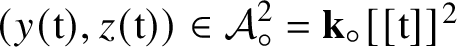 $(y(\mathrm {t}),z(\mathrm {t}))\in \mathcal A_{\circ }^2=\mathbf {k}_{\circ }[[\mathrm {t}]]^2$
satisfying the quadratic equation
$(y(\mathrm {t}),z(\mathrm {t}))\in \mathcal A_{\circ }^2=\mathbf {k}_{\circ }[[\mathrm {t}]]^2$
satisfying the quadratic equation
 $$ \begin{align*} f(\mathrm{t},y(\mathrm{t}),z(\mathrm{t}))=y(\mathrm{t})^2 -2\mathrm{t}\cdot y(\mathrm{t})\cdot z(\mathrm{t})^2+\mathrm{t}^4=0. \end{align*} $$
One may solve for y in terms of z and get
 $$ \begin{align*} y(\mathrm{t})=\mathrm{t}\cdot z(\mathrm{t})\pm \mathrm{t}\cdot \sqrt{z(\mathrm{t})^4-\mathrm{t}^2}. \end{align*} $$
The root
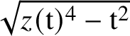 $\sqrt {z(\mathrm {t})^4-\mathrm {t}^2}$
is a formal power series in
$\sqrt {z(\mathrm {t})^4-\mathrm {t}^2}$
is a formal power series in
 $\mathrm {t}$
of order
$\mathrm {t}$
of order
 $1$
for any series
$1$
for any series
 $z(\mathrm {t})\in \mathcal A_{\circ }$
.
$z(\mathrm {t})\in \mathcal A_{\circ }$
.
There is a natural way to define the arquile regular and singular loci
 $\mathrm {Arq.Reg}({\mathcal Y})$
and
$\mathrm {Arq.Reg}({\mathcal Y})$
and
 $\mathrm {Arq.Sing}({\mathcal Y})$
of an arquile variety
$\mathrm {Arq.Sing}({\mathcal Y})$
of an arquile variety
 ${\mathcal Y}={\mathcal Y}(f)$
Footnote
8
: Let
${\mathcal Y}={\mathcal Y}(f)$
Footnote
8
: Let
 $I=I_{\mathcal Y}$
be the ideal of
$I=I_{\mathcal Y}$
be the ideal of
 ${\mathcal B}$
of power series
${\mathcal B}$
of power series
 $f(\mathrm {t},\mathrm {y})$
vanishing on
$f(\mathrm {t},\mathrm {y})$
vanishing on
 ${\mathcal Y}$
, say
${\mathcal Y}$
, say
 $f(\mathrm {t},y(\mathrm {t}))=0$
for all
$f(\mathrm {t},y(\mathrm {t}))=0$
for all
 $y\in {\mathcal Y}$
. For a point y of
$y\in {\mathcal Y}$
. For a point y of
 ${\mathcal Y}$
, denote by
${\mathcal Y}$
, denote by
 ${\mathcal P}_y$
the prime ideal of
${\mathcal P}_y$
the prime ideal of
 ${\mathcal B}$
of power series
${\mathcal B}$
of power series
 $f(\mathrm {t},\mathrm {y})$
vanishing at y,
$f(\mathrm {t},\mathrm {y})$
vanishing at y,
 $$ \begin{align*} {\mathcal P}_y= \{f\in{\mathcal B},\, f(\mathrm{t},y(\mathrm{t}))=0\}. \end{align*} $$
Let
 ${\mathcal B}_{{\mathcal P}_y}$
be the localisation of
${\mathcal B}_{{\mathcal P}_y}$
be the localisation of
 ${\mathcal B}$
at
${\mathcal B}$
at
 ${\mathcal P}_y$
. This is a Noetherian ring in the formal, convergent and algebraic setting.Footnote
9
Then
${\mathcal P}_y$
. This is a Noetherian ring in the formal, convergent and algebraic setting.Footnote
9
Then
 ${\mathcal Y}$
is called arquile regular at y, or y is called an arq.regular point of
${\mathcal Y}$
is called arquile regular at y, or y is called an arq.regular point of
 ${\mathcal Y}$
, if the factor ring
${\mathcal Y}$
, if the factor ring
 $$ \begin{align*} {\mathcal B}_{{\mathcal P}_y}/I\cdot{\mathcal B}_{{\mathcal P}_y} \end{align*} $$
is a regular local ring. Otherwise,
 ${\mathcal Y}$
is called arquile singular at y. We set
${\mathcal Y}$
is called arquile singular at y. We set
 $\mathrm {Arq.Reg}=\{y\in {\mathcal Y},\, y$
arq.regular point of
$\mathrm {Arq.Reg}=\{y\in {\mathcal Y},\, y$
arq.regular point of
 ${\mathcal Y}\}$
and
${\mathcal Y}\}$
and
 $\mathrm {Arq.Sing}({\mathcal Y})={\mathcal Y}\setminus \mathrm {Arq.Reg}({\mathcal Y})$
.
$\mathrm {Arq.Sing}({\mathcal Y})={\mathcal Y}\setminus \mathrm {Arq.Reg}({\mathcal Y})$
.
If
 ${\mathcal Y}=X_{\infty ,0}$
is the space of arcs centred at
${\mathcal Y}=X_{\infty ,0}$
is the space of arcs centred at
 $0$
of an algebraic subvariety X of
$0$
of an algebraic subvariety X of
 $\mathbb A^m_{\mathbf {k}}$
, a point
$\mathbb A^m_{\mathbf {k}}$
, a point
 $y\in {\mathcal Y}$
is arq.regular if and only if the image of y in X (i.e., the generic point of y) does not lie entirely in the singular locus of X; that is, if
$y\in {\mathcal Y}$
is arq.regular if and only if the image of y in X (i.e., the generic point of y) does not lie entirely in the singular locus of X; that is, if
 $y\not \in (\mathrm {Sing}\, X)_{\infty ,0}$
. This condition appears naturally in the theory of arc spaces; see, for example, [Reference Grinberg and KazhdanGK, Reference DrinfeldDr, Reference Denef and LoeserDL, Reference Bourqui and SebagBS1, Reference Bourqui and SebagBS2, Reference BouthierBou, Reference de Fernex, Ein and IshiidFEI, Reference Chambert-Loir, Nicaise and SebagCNS].
$y\not \in (\mathrm {Sing}\, X)_{\infty ,0}$
. This condition appears naturally in the theory of arc spaces; see, for example, [Reference Grinberg and KazhdanGK, Reference DrinfeldDr, Reference Denef and LoeserDL, Reference Bourqui and SebagBS1, Reference Bourqui and SebagBS2, Reference BouthierBou, Reference de Fernex, Ein and IshiidFEI, Reference Chambert-Loir, Nicaise and SebagCNS].
Our first result is the description of the
 $\mathrm {t}$
-adically local geometry of arquile varieties (see Theorems 2.6 and 8.1 for the precise statements).
$\mathrm {t}$
-adically local geometry of arquile varieties (see Theorems 2.6 and 8.1 for the precise statements).
Theorem 1.2. Arq.regular and arq.singular points
Let
 ${\mathcal Y}={\mathcal Y}(f)$
be an arquile variety in
${\mathcal Y}={\mathcal Y}(f)$
be an arquile variety in
 $\mathcal A_{\circ }^m$
, where
$\mathcal A_{\circ }^m$
, where
 $\mathcal A_{\circ }$
denotes one of the rings
$\mathcal A_{\circ }$
denotes one of the rings
 $\mathbf {k}_{\circ }[[\mathrm {t}]]$
,
$\mathbf {k}_{\circ }[[\mathrm {t}]]$
,
 $\mathbf {k}_{\circ }\{\mathrm {t}\}$
or
$\mathbf {k}_{\circ }\{\mathrm {t}\}$
or
 $\mathbf {k}_{\circ }\langle \mathrm {t}\rangle $
and where
$\mathbf {k}_{\circ }\langle \mathrm {t}\rangle $
and where
 $f\in {\mathcal B}^k$
is a power series vector in
$f\in {\mathcal B}^k$
is a power series vector in
 $\mathrm {t}$
and
$\mathrm {t}$
and
 $\mathrm {y}_1,\ldots ,\mathrm {y}_m$
of the same quality as
$\mathrm {y}_1,\ldots ,\mathrm {y}_m$
of the same quality as
 $\mathcal A_{\circ }$
.Footnote
10
$\mathcal A_{\circ }$
.Footnote
10
(a) The arquile singular locus
 $\mathrm {Arq.Sing}({\mathcal Y})$
of
$\mathrm {Arq.Sing}({\mathcal Y})$
of
 ${\mathcal Y}$
is an arquile closed, proper subset of
${\mathcal Y}$
is an arquile closed, proper subset of
 ${\mathcal Y}$
. It can be defined in
${\mathcal Y}$
. It can be defined in
 ${\mathcal Y}$
by the vanishing of appropriate minors
${\mathcal Y}$
by the vanishing of appropriate minors
 $g_j(\mathrm {t},\mathrm {y})$
,
$g_j(\mathrm {t},\mathrm {y})$
,
 $j=1,\ldots ,q$
, of the relative Jacobian matrix
$j=1,\ldots ,q$
, of the relative Jacobian matrix
 ${\partial }_{\mathrm {y}} f(\mathrm {t},\mathrm {y})$
of f,
${\partial }_{\mathrm {y}} f(\mathrm {t},\mathrm {y})$
of f,
 $$ \begin{align*} \mathrm{Arq.Sing}({\mathcal Y})=\{y(\mathrm{t})\in{\mathcal Y},\, g_1(\mathrm{t},y(\mathrm{t}))=\ldots =g_q(\mathrm{t},y(\mathrm{t}))=0\}. \end{align*} $$
(b) Every arq.regular point
 $y\in \mathrm {Arq.Reg}({\mathcal Y})$
of
$y\in \mathrm {Arq.Reg}({\mathcal Y})$
of
 ${\mathcal Y}$
has a
${\mathcal Y}$
has a
 $\mathrm {t}$
-adically open and textile locally closed neighbourhood
$\mathrm {t}$
-adically open and textile locally closed neighbourhood
 ${\mathcal {W}}$
which is textile isomorphic to a free
${\mathcal {W}}$
which is textile isomorphic to a free
 $\mathcal A_{\circ }$
-module
$\mathcal A_{\circ }$
-module
 $\mathcal A_{\circ }^s$
,
$\mathcal A_{\circ }^s$
,
 $$ \begin{align*} \Phi:{\mathcal{W}}\,\,\smash{\mathop{\longrightarrow}\limits^{\cong}}\,\, \mathcal A_{\circ}^s. \end{align*} $$
Remarks 1.3. (a) It follows from assertion (a) that the iterated arq.singular loci
 $\,\mathrm {Arq.Sing}_{i+1}({\mathcal Y})=\mathrm {Arq.Sing}(\mathrm {Arq.Sing}_i({\mathcal Y}))$
of
$\,\mathrm {Arq.Sing}_{i+1}({\mathcal Y})=\mathrm {Arq.Sing}(\mathrm {Arq.Sing}_i({\mathcal Y}))$
of
 ${\mathcal Y}$
, with
${\mathcal Y}$
, with
 $\mathrm {Arq.Sing}_0({\mathcal Y})={\mathcal Y}$
, define a finite filtration of
$\mathrm {Arq.Sing}_0({\mathcal Y})={\mathcal Y}$
, define a finite filtration of
 ${\mathcal Y}$
by arquile closed subvarieties. Their set-theoretic differences admit the analogous local description as
${\mathcal Y}$
by arquile closed subvarieties. Their set-theoretic differences admit the analogous local description as
 ${\mathcal Y}$
.
${\mathcal Y}$
.
(b) Assertion (b) says that
 $\mathrm {t}$
-adic locally at an arq.regular point y of
$\mathrm {t}$
-adic locally at an arq.regular point y of
 ${\mathcal Y}$
, an arquile variety is ‘smooth’ in the sense of differential geometry. The neighbourhood
${\mathcal Y}$
, an arquile variety is ‘smooth’ in the sense of differential geometry. The neighbourhood
 ${\mathcal {W}}$
and the isomorphim
${\mathcal {W}}$
and the isomorphim
 $\Phi $
are constructed explicitly in the proof. In general, it seems that the neighbourhood
$\Phi $
are constructed explicitly in the proof. In general, it seems that the neighbourhood
 ${\mathcal {W}}$
cannot be chosen arquile open or at least textile open; cf. [Reference Bourqui and SebagBS3]. As
${\mathcal {W}}$
cannot be chosen arquile open or at least textile open; cf. [Reference Bourqui and SebagBS3]. As
 $\Phi $
is a textile isomorphism, it is also a
$\Phi $
is a textile isomorphism, it is also a
 $\mathrm {t}$
-adic homeomorphism.
$\mathrm {t}$
-adic homeomorphism.
Assertion (b) of the preceding theorem is a consequence of the principal result of this article, which describes the arquile local geometry of arquile varieties. The arquile topology is coarser than the
 $\mathrm {t}$
-adic topology appearing in Theorem 1.2, so the statements below are stronger (see Theorem 7.1 for a more detailed statement). Results of a similar flavour have been obtained by Bouthier for arc spaces [Reference BouthierBou]. However, the arguments and the formulation of the results there are somewhat different from ours; it would be interesting to figure out the precise relation between the two approaches.
$\mathrm {t}$
-adic topology appearing in Theorem 1.2, so the statements below are stronger (see Theorem 7.1 for a more detailed statement). Results of a similar flavour have been obtained by Bouthier for arc spaces [Reference BouthierBou]. However, the arguments and the formulation of the results there are somewhat different from ours; it would be interesting to figure out the precise relation between the two approaches.
Theorem 1.4. Structure of arquile varieties
Let
 ${\mathcal Y}={\mathcal Y}(f)$
be an arquile variety in
${\mathcal Y}={\mathcal Y}(f)$
be an arquile variety in
 $\mathcal A_{\circ }^m$
, where
$\mathcal A_{\circ }^m$
, where
 $\mathcal A_{\circ }$
denotes one of the rings
$\mathcal A_{\circ }$
denotes one of the rings
 $\mathbf {k}_{\circ }[[\mathrm {t}]]$
,
$\mathbf {k}_{\circ }[[\mathrm {t}]]$
,
 $\mathbf {k}_{\circ }\{\mathrm {t}\}$
,
$\mathbf {k}_{\circ }\{\mathrm {t}\}$
,
 $\mathbf {k}_{\circ }\{\mathrm {t}\}_s$
or
$\mathbf {k}_{\circ }\{\mathrm {t}\}_s$
or
 $\mathbf {k}_{\circ }\langle \mathrm {t}\rangle $
and where
$\mathbf {k}_{\circ }\langle \mathrm {t}\rangle $
and where
 $f\in {\mathcal B}^k$
is a power series vector in
$f\in {\mathcal B}^k$
is a power series vector in
 $\mathrm {t}$
and
$\mathrm {t}$
and
 $\mathrm {y}_1,\ldots ,\mathrm {y}_m$
of the same quality as
$\mathrm {y}_1,\ldots ,\mathrm {y}_m$
of the same quality as
 $\mathcal A_{\circ }$
. Cover the arquile regular locus
$\mathcal A_{\circ }$
. Cover the arquile regular locus
 $\mathrm {Arq.Reg}({\mathcal Y})$
of
$\mathrm {Arq.Reg}({\mathcal Y})$
of
 ${\mathcal Y}$
by the arquile open subsets
${\mathcal Y}$
by the arquile open subsets
 $$ \begin{align*} {\mathcal U}_j=\{y(\mathrm{t})\in{\mathcal Y},\, g_j(\mathrm{t},y(\mathrm{t}))\neq 0\}, \end{align*} $$
where
 $g_1(\mathrm {t},\mathrm {y}),\ldots ,g_q(\mathrm {t},\mathrm {y})$
denote minors of the relative Jacobian matrix
$g_1(\mathrm {t},\mathrm {y}),\ldots ,g_q(\mathrm {t},\mathrm {y})$
denote minors of the relative Jacobian matrix
 ${\partial }_{\mathrm {y}} f(\mathrm {t},\mathrm {y})$
of f defining
${\partial }_{\mathrm {y}} f(\mathrm {t},\mathrm {y})$
of f defining
 $\mathrm {Arq.Sing}({\mathcal Y})$
as in Theorem 1.2. For
$\mathrm {Arq.Sing}({\mathcal Y})$
as in Theorem 1.2. For
 $j=1,\ldots ,q$
and
$j=1,\ldots ,q$
and
 $d\in {\mathbb N}$
, let
$d\in {\mathbb N}$
, let
 $$ \begin{align*} {\mathcal Y}_{jd}=\{y(\mathrm{t})\in{\mathcal U}_j,\, \mathrm{ord}_{\mathrm{t}}\, g_j(\mathrm{t},y(\mathrm{t}))=d\} \end{align*} $$
denote the textile locally closed stratum in
 ${\mathcal U}_{j}$
of vectors
${\mathcal U}_{j}$
of vectors
 $y(\mathrm {t})$
for which
$y(\mathrm {t})$
for which
 $g_{j}(\mathrm {t},y(\mathrm {t}))$
has order d as a series in
$g_{j}(\mathrm {t},y(\mathrm {t}))$
has order d as a series in
 $\mathrm {t}$
. Then each
$\mathrm {t}$
. Then each
 ${\mathcal Y}_{jd}$
is (naturally) textile isomorphic to a Cartesian product of a (finite-dimensional) algebraic variety
${\mathcal Y}_{jd}$
is (naturally) textile isomorphic to a Cartesian product of a (finite-dimensional) algebraic variety
 ${\mathcal Z}_{jd}$
with a free
${\mathcal Z}_{jd}$
with a free
 $\mathcal A_{\circ }$
-module
$\mathcal A_{\circ }$
-module
 $\mathcal A_{\circ }^{s}$
,
$\mathcal A_{\circ }^{s}$
,
 $$ \begin{align*} \Phi_{jd}: {\mathcal Y}_{jd}\,\,\smash{\mathop{\longrightarrow}\limits^{\cong}}\,\, {\mathcal Z}_{jd}\times \mathcal A_{\circ}^{s}. \end{align*} $$
Remarks 1.5. (a) It is necessary for the factorisation to cover
 ${\mathcal Y}$
first by the arquile open sets
${\mathcal Y}$
first by the arquile open sets
 ${\mathcal U}_j$
and to then work with each
${\mathcal U}_j$
and to then work with each
 ${\mathcal U}_j$
individually. These are countable unions of the strata
${\mathcal U}_j$
individually. These are countable unions of the strata
 ${\mathcal Y}_{jd}$
, for
${\mathcal Y}_{jd}$
, for
 $d\in {\mathbb N}$
, and each
$d\in {\mathbb N}$
, and each
 ${\mathcal Y}_{jd}$
can be factorised as indicated above. By assertion (a) of Theorem 1.2, the covering and factorisation of the arq.regular locus of
${\mathcal Y}_{jd}$
can be factorised as indicated above. By assertion (a) of Theorem 1.2, the covering and factorisation of the arq.regular locus of
 ${\mathcal Y}$
can be repeated for the arquile locally closed strata
${\mathcal Y}$
can be repeated for the arquile locally closed strata
 ${\mathcal Y}_i=\mathrm {Arq.Sing}_i({\mathcal Y})\setminus \mathrm {Arq.Sing}_{i+1}({\mathcal Y})$
of the arq.regular points of
${\mathcal Y}_i=\mathrm {Arq.Sing}_i({\mathcal Y})\setminus \mathrm {Arq.Sing}_{i+1}({\mathcal Y})$
of the arq.regular points of
 $\mathrm {Arq.Sing}_i({\mathcal Y})$
.
$\mathrm {Arq.Sing}_i({\mathcal Y})$
.
(b) The varieties
 ${\mathcal Z}_{jd}$
are in general singular (some of them may be empty). They can be equipped naturally with a (not necessarily reduced) scheme structure. All strata and isomorphisms will be constructed explicitly. The textile isomorphisms
${\mathcal Z}_{jd}$
are in general singular (some of them may be empty). They can be equipped naturally with a (not necessarily reduced) scheme structure. All strata and isomorphisms will be constructed explicitly. The textile isomorphisms
 $\Phi _{jd}$
are compositions of a division map with an arquile map and are, in particular,
$\Phi _{jd}$
are compositions of a division map with an arquile map and are, in particular,
 $\mathrm {t}$
-adic homeomorphisms. The smooth factor
$\mathrm {t}$
-adic homeomorphisms. The smooth factor
 $\mathcal A_{\circ }^{s}$
appears naturally through the construction of the map
$\mathcal A_{\circ }^{s}$
appears naturally through the construction of the map
 $\Phi _{jd}$
though it is abstractly textile isomorphic to
$\Phi _{jd}$
though it is abstractly textile isomorphic to
 $\mathcal A_{\circ }$
; the chosen factor will be the same for all j and d.
$\mathcal A_{\circ }$
; the chosen factor will be the same for all j and d.
(c) For convergent
 $y(\mathrm {t})$
and f, the isomorphisms
$y(\mathrm {t})$
and f, the isomorphisms
 $\Phi _{jd}$
are analytic in the sense of locally convex spaces; see [Reference Hauser and MüllerHM]. In the case where
$\Phi _{jd}$
are analytic in the sense of locally convex spaces; see [Reference Hauser and MüllerHM]. In the case where
 $\mathcal A_{\circ }=\mathbf {k}_{\circ }\{\mathrm {t}\}_s$
, for
$\mathcal A_{\circ }=\mathbf {k}_{\circ }\{\mathrm {t}\}_s$
, for
 $s>0$
, the statement of the theorem has to be slightly modified: First, it holds only for radii s which are sufficiently small with respect to the given f and, secondly, one has to restrict
$s>0$
, the statement of the theorem has to be slightly modified: First, it holds only for radii s which are sufficiently small with respect to the given f and, secondly, one has to restrict
 ${\mathcal Y}_{jd}$
to a sufficiently small ball with respect to the s-norm. The isomorphisms
${\mathcal Y}_{jd}$
to a sufficiently small ball with respect to the s-norm. The isomorphisms
 $\Phi _{jd}$
are then Banach-analytic. This relates to the theory of short arcs, in particular to a question of Kollár-Némethi; see Conjecture 73 in [Reference Kollár and NémethiKN], as well as [Reference Johnson and KollárJK, Reference BouthierBou].
$\Phi _{jd}$
are then Banach-analytic. This relates to the theory of short arcs, in particular to a question of Kollár-Némethi; see Conjecture 73 in [Reference Kollár and NémethiKN], as well as [Reference Johnson and KollárJK, Reference BouthierBou].
(d) It is not hard to see that the theorem implies assertion (b) of Theorem 1.2 by applying it to
 ${\mathcal Y}^{\circ }:=\mathrm {Arq.Reg}({\mathcal Y})$
, the set of arq.regular points of
${\mathcal Y}^{\circ }:=\mathrm {Arq.Reg}({\mathcal Y})$
, the set of arq.regular points of
 ${\mathcal Y}$
, and taking a sufficiently small
${\mathcal Y}$
, and taking a sufficiently small
 $\mathrm {t}$
-adic neighbourhood
$\mathrm {t}$
-adic neighbourhood
 ${\mathcal {W}}$
of the arq.regular point y such that
${\mathcal {W}}$
of the arq.regular point y such that
 $\Phi _{jd}$
maps
$\Phi _{jd}$
maps
 ${\mathcal {W}}$
to
${\mathcal {W}}$
to
 $\{0\}\times \mathcal A_{\circ }^{s}$
. Note that
$\{0\}\times \mathcal A_{\circ }^{s}$
. Note that
 ${\mathcal {W}}$
can be taken
${\mathcal {W}}$
can be taken
 $\mathrm {t}$
-adic open because of (a) of Theorem 1.2.
$\mathrm {t}$
-adic open because of (a) of Theorem 1.2.
The proof of Theorem 1.4 is based on a geometric interpretation of the proofs of Artin and Płoski of their respective approximation theorems for the power series solutions of formal and analytic equations [Reference ArtinAr1, Reference ArtinAr2, Reference PłoskiPł]. This geometric viewpoint allows us to transfer linearisation techniques from differential geometry to the context of arquile maps between power series spaces: the defining equations of the strata
 ${\mathcal Y}_{jd}$
will be linearised up to a finite-dimensional subspace of
${\mathcal Y}_{jd}$
will be linearised up to a finite-dimensional subspace of
 $\mathcal A_{\circ }^m$
by composing them with suitable textile isomorphisms; see Theorem 1.9. The linear part of the equations defines the smooth factor
$\mathcal A_{\circ }^m$
by composing them with suitable textile isomorphisms; see Theorem 1.9. The linear part of the equations defines the smooth factor
 $\mathcal A_{\circ }^{s}$
, the nonlinear part the variety
$\mathcal A_{\circ }^{s}$
, the nonlinear part the variety
 ${\mathcal Z}_{jd}$
. The linearisation of the defining equations of
${\mathcal Z}_{jd}$
. The linearisation of the defining equations of
 ${\mathcal Y}_{jd}$
shows that the trivialising isomorphisms
${\mathcal Y}_{jd}$
shows that the trivialising isomorphisms
 $\Phi _{jd}$
of the structure theorem are actually embedded (i.e., stem from isomorphisms of (suitable strata of) the affine ambient space
$\Phi _{jd}$
of the structure theorem are actually embedded (i.e., stem from isomorphisms of (suitable strata of) the affine ambient space
 $\mathcal A_{\circ }^m$
) and, moreover, induce a natural scheme structure on the finite-dimensional factor
$\mathcal A_{\circ }^m$
) and, moreover, induce a natural scheme structure on the finite-dimensional factor
 ${\mathcal Z}_{jd}$
.
${\mathcal Z}_{jd}$
.
As a direct consequence of the structure theorem, one obtains Artin’s analytic, algebraic and strong approximation theorems in the univariate case in the following version; cf. [Reference ArtinAr1, Reference ArtinAr2, Reference PłoskiPł, Reference GreenbergGre].
Corollary 1.6. (a) Let
 $f(\mathrm {t},\mathrm {y})$
be a convergent, respectively algebraic, power series vector. The sets of convergent, respectively algebraic, power series solutions
$f(\mathrm {t},\mathrm {y})$
be a convergent, respectively algebraic, power series vector. The sets of convergent, respectively algebraic, power series solutions
 $y(\mathrm {t})\in \mathbf {k}_{\circ }\{\mathrm {t}\}^m$
, respectively
$y(\mathrm {t})\in \mathbf {k}_{\circ }\{\mathrm {t}\}^m$
, respectively
 $y(\mathrm {t})\in \mathbf {k}_{\circ }\langle \mathrm {t}\rangle ^m$
, of
$y(\mathrm {t})\in \mathbf {k}_{\circ }\langle \mathrm {t}\rangle ^m$
, of
 $f(\mathrm {t},\mathrm {y})=0$
are
$f(\mathrm {t},\mathrm {y})=0$
are
 $\mathrm {t}$
-adically dense in the set of formal power series solutions
$\mathrm {t}$
-adically dense in the set of formal power series solutions
 $\widehat y(\mathrm {t})\in \mathbf {k}_{\circ }[[\mathrm {t}]]^m$
.
$\widehat y(\mathrm {t})\in \mathbf {k}_{\circ }[[\mathrm {t}]]^m$
.
(b) Let f be a formal power series vector. For all
 $c\in {\mathbb N}$
, every
$c\in {\mathbb N}$
, every
 $\mathrm {t}$
-adically sufficiently good approximate solution
$\mathrm {t}$
-adically sufficiently good approximate solution
 $\overline y(\mathrm {t})$
of
$\overline y(\mathrm {t})$
of
 $f(\mathrm {t},\mathrm {y})=0$
admits an exact formal solution
$f(\mathrm {t},\mathrm {y})=0$
admits an exact formal solution
 $\widehat y(\mathrm {t})$
which coincides with
$\widehat y(\mathrm {t})$
which coincides with
 $\overline y(\mathrm {t})$
up to degree c.
$\overline y(\mathrm {t})$
up to degree c.
Indeed, the structure theorem reduces the approximation problem to the case of linear equations, and there the flatness of the formal power series ring over the rings of convergent and algebraic power series implies the existence of the respective power series solutions; see Remark 5.7 for the details of this reasoning. This method also works for power series in several variables and provides a ‘geometric’ proof for Artin approximation. The technicalities are, however, more involved [Reference HauserHa2].
Formally local geometry. There is a second, more deformation-theoretic approach to the geometry of arquile varieties: Instead of decomposing them into strata which are shown to be ‘globally’ Cartesian products, one can also study the germs or formal neighbourhoods of arquile varieties
 ${\mathcal Y}$
at selected arq.regular points y. This corresponds to work with the local rings
${\mathcal Y}$
at selected arq.regular points y. This corresponds to work with the local rings
 ${\mathcal O}_{{\mathcal Y},y}$
of
${\mathcal O}_{{\mathcal Y},y}$
of
 ${\mathcal Y}$
at y (as defined below) and their completions
${\mathcal Y}$
at y (as defined below) and their completions
 $\widehat {\mathcal O}_{{\mathcal Y},y}$
. The respective result, first established by Grinberg–Kazhdan and Drinfeld in the special case of arc spaces, can be understood as a partial generalisation of Cohen’s structure theorem to the infinite-dimensional setting: Cohen’s theorem asserts that a complete local Noetherian ring S containing a field is isomorphic to a factor ring of a ring of formal power series in finitely many variables over this field; see Theorem 29.7 in [Reference MatsumuraMa]. And S is regular if and only if it is isomorphic to a ring of formal power series in finitely many variables. In the infinite-dimensional context, the statement is more complicated – see Theorem 1.7 – and only provides a description of the rings
$\widehat {\mathcal O}_{{\mathcal Y},y}$
. The respective result, first established by Grinberg–Kazhdan and Drinfeld in the special case of arc spaces, can be understood as a partial generalisation of Cohen’s structure theorem to the infinite-dimensional setting: Cohen’s theorem asserts that a complete local Noetherian ring S containing a field is isomorphic to a factor ring of a ring of formal power series in finitely many variables over this field; see Theorem 29.7 in [Reference MatsumuraMa]. And S is regular if and only if it is isomorphic to a ring of formal power series in finitely many variables. In the infinite-dimensional context, the statement is more complicated – see Theorem 1.7 – and only provides a description of the rings
 $\widehat {\mathcal O}_{{\mathcal Y},y}$
for arq.regular points y of
$\widehat {\mathcal O}_{{\mathcal Y},y}$
for arq.regular points y of
 ${\mathcal Y}$
. A different formulation in terms of deformations is given in Theorem 10.2.
${\mathcal Y}$
. A different formulation in terms of deformations is given in Theorem 10.2.
We restrict in the statement below to the case of formal power series. An analogous statement holds for convergent power series, considering
 $\mathbf {k}_{\circ }\{\mathrm {t}\}$
as the inductive limit of the Banach spaces
$\mathbf {k}_{\circ }\{\mathrm {t}\}$
as the inductive limit of the Banach spaces
 $\mathbf {k}_{\circ }\{\mathrm {t}\}_s$
, for
$\mathbf {k}_{\circ }\{\mathrm {t}\}_s$
, for
 $s>0$
, as in [Reference Grauert and RemmertGR, Reference Hauser and MüllerHM]. Vectors
$s>0$
, as in [Reference Grauert and RemmertGR, Reference Hauser and MüllerHM]. Vectors
 $y(\mathrm {t})=(y_1(\mathrm {t}),\ldots ,y_m(\mathrm {t}))\in \mathcal A_{\circ }^m$
will be expanded componentwise into
$y(\mathrm {t})=(y_1(\mathrm {t}),\ldots ,y_m(\mathrm {t}))\in \mathcal A_{\circ }^m$
will be expanded componentwise into
 $y_i(\mathrm {t})=\sum _{j\geq 1} y_{ij}\cdot \mathrm {t}^j$
with coefficients
$y_i(\mathrm {t})=\sum _{j\geq 1} y_{ij}\cdot \mathrm {t}^j$
with coefficients
 $y_{ij}\in \mathbf {k}^m$
. Let as above
$y_{ij}\in \mathbf {k}^m$
. Let as above
 $\mathbf { k}[\mathrm {y}_{m,\infty }]$
denote the polynomial ring in countably many variables
$\mathbf { k}[\mathrm {y}_{m,\infty }]$
denote the polynomial ring in countably many variables
 $\mathrm {y}_{ij}$
, for
$\mathrm {y}_{ij}$
, for
 $1\leq i\leq m$
and
$1\leq i\leq m$
and
 $j\geq 1$
. If
$j\geq 1$
. If
 ${\mathcal Y}={\mathcal Y}(I)$
is an arquile variety in
${\mathcal Y}={\mathcal Y}(I)$
is an arquile variety in
 $\mathcal A_{\circ }^m$
defined by the ideal I of
$\mathcal A_{\circ }^m$
defined by the ideal I of
 ${\mathcal B}$
, the elements of I induce, by comparison of the coefficients of
${\mathcal B}$
, the elements of I induce, by comparison of the coefficients of
 $\mathrm {t}^{\ell }$
, polynomials
$\mathrm {t}^{\ell }$
, polynomials
 $F_{\ell }\in \mathbf {k}[\mathrm {y}_{m,\infty }]$
,
$F_{\ell }\in \mathbf {k}[\mathrm {y}_{m,\infty }]$
,
 $\ell \in {\mathbb N}$
, which define the equations between the coefficients
$\ell \in {\mathbb N}$
, which define the equations between the coefficients
 $y_{ij}$
of points y of
$y_{ij}$
of points y of
 ${\mathcal Y}$
. Denote by
${\mathcal Y}$
. Denote by
 $I_{\infty }$
the resulting ideal of
$I_{\infty }$
the resulting ideal of
 $\mathbf {k}[\mathrm {y}_{m,\infty }]$
, so that
$\mathbf {k}[\mathrm {y}_{m,\infty }]$
, so that
 $\mathbf {k}[\mathrm {y}_{m,\infty }]/I_{\infty }$
is the (infinite-dimensional) coordinate ring of
$\mathbf {k}[\mathrm {y}_{m,\infty }]/I_{\infty }$
is the (infinite-dimensional) coordinate ring of
 ${\mathcal Y}$
. Let
${\mathcal Y}$
. Let
 $M_{y,\infty }$
be the maximal ideal of
$M_{y,\infty }$
be the maximal ideal of
 $\mathbf {k}[\mathrm {y}_{m,\infty }]$
generated by all
$\mathbf {k}[\mathrm {y}_{m,\infty }]$
generated by all
 $\mathrm {y}_{ij}-y_{ij}$
, for
$\mathrm {y}_{ij}-y_{ij}$
, for
 $1\leq i\leq m$
and
$1\leq i\leq m$
and
 $j\geq 1$
, and let
$j\geq 1$
, and let
 $N_{y,\infty }$
be its image in
$N_{y,\infty }$
be its image in
 $\mathbf {k}[\mathrm {y}_{m,\infty }]/I_{\infty }$
. The local ring
$\mathbf {k}[\mathrm {y}_{m,\infty }]/I_{\infty }$
. The local ring
 ${\mathcal O}_{{\mathcal Y},y}$
of
${\mathcal O}_{{\mathcal Y},y}$
of
 ${\mathcal Y}$
at y is given by the localisation
${\mathcal Y}$
at y is given by the localisation
 $$ \begin{align*} {\mathcal O}_{{\mathcal Y},y}=(\mathbf{k}[\mathrm{y}_{m,\infty}]/I_{\infty})_{N_{y,\infty}}. \end{align*} $$
Let
 $\widehat {\mathcal O}_{{\mathcal Y},y}=\varprojlim \, {\mathcal O}_{{\mathcal Y},y}/N_{y,\infty }^k$
be the inverse limit of the factor rings
$\widehat {\mathcal O}_{{\mathcal Y},y}=\varprojlim \, {\mathcal O}_{{\mathcal Y},y}/N_{y,\infty }^k$
be the inverse limit of the factor rings
 ${\mathcal O}_{{\mathcal Y},y}/N_{y,\infty }^k$
.Footnote
11
We call this ring the completed local ring of
${\mathcal O}_{{\mathcal Y},y}/N_{y,\infty }^k$
.Footnote
11
We call this ring the completed local ring of
 ${\mathcal Y}$
at y. It defines the formal neighbourhood
${\mathcal Y}$
at y. It defines the formal neighbourhood
 $(\widehat {{\mathcal Y},y})$
of y in
$(\widehat {{\mathcal Y},y})$
of y in
 ${\mathcal Y}$
.
${\mathcal Y}$
.
Theorem 1.7. Grinberg–Kazhdan–Drinfeld factorisation theorem
Let
 ${\mathcal Y}={\mathcal Y}(f)\subset \mathcal A_{\circ }^m$
be an arquile variety defined by a polynomial vector
${\mathcal Y}={\mathcal Y}(f)\subset \mathcal A_{\circ }^m$
be an arquile variety defined by a polynomial vector
 $f(\mathrm {t},\mathrm {y})$
, and let
$f(\mathrm {t},\mathrm {y})$
, and let
 $y=y(\mathrm {t})$
be an arq.regular point of
$y=y(\mathrm {t})$
be an arq.regular point of
 ${\mathcal Y}$
. Then the completed local ring
${\mathcal Y}$
. Then the completed local ring
 $\widehat {\mathcal O}_{{\mathcal Y},y}$
is isomorphic to a formal power series ring
$\widehat {\mathcal O}_{{\mathcal Y},y}$
is isomorphic to a formal power series ring
 $C[[\mathrm {v}_{\infty }]] =C[[\mathrm {v}_1,\mathrm {v}_2,\ldots ]]$
in countably many variables with coefficients in a
$C[[\mathrm {v}_{\infty }]] =C[[\mathrm {v}_1,\mathrm {v}_2,\ldots ]]$
in countably many variables with coefficients in a
 $\mathbf {k}$
-algebra C which is the completion of a localisation of a
$\mathbf {k}$
-algebra C which is the completion of a localisation of a
 $\mathbf {k}$
-algebra of finite type,
$\mathbf {k}$
-algebra of finite type,
 $$ \begin{align*} \widehat{\mathcal O}_{{\mathcal Y},y}\cong C[[\mathrm{v}_{\infty}]]. \end{align*} $$
Remark 1.8. The ring
 $\widehat {\mathcal O}_{{\mathcal Y},y}$
can be characterised by deformations of y over test-algebras (local algebras with nilpotent maximal ideals), and this is how Grinberg–Kazhdan and Drinfeld prove the respective factorisation result [Reference Grinberg and KazhdanGK, Reference DrinfeldDr, Reference Bruschek and HauserBH]. Additional information on this result can be found in [Reference Bourqui and SebagBS1, Reference BouthierBou, Reference Bouthier, Ngô and SakellaridisBNS, Reference Chambert-Loir, Nicaise and SebagCNS, Reference Nicaise and SebagNS]. In the present text, we will establish the factorisation more generally for all deformations of y, with parameters varying in an arbitrary complete local ring S (the topology of S need not be defined by the powers of an ideal); see Theorem 10.2 for the precise formulation.Footnote
12
$\widehat {\mathcal O}_{{\mathcal Y},y}$
can be characterised by deformations of y over test-algebras (local algebras with nilpotent maximal ideals), and this is how Grinberg–Kazhdan and Drinfeld prove the respective factorisation result [Reference Grinberg and KazhdanGK, Reference DrinfeldDr, Reference Bruschek and HauserBH]. Additional information on this result can be found in [Reference Bourqui and SebagBS1, Reference BouthierBou, Reference Bouthier, Ngô and SakellaridisBNS, Reference Chambert-Loir, Nicaise and SebagCNS, Reference Nicaise and SebagNS]. In the present text, we will establish the factorisation more generally for all deformations of y, with parameters varying in an arbitrary complete local ring S (the topology of S need not be defined by the powers of an ideal); see Theorem 10.2 for the precise formulation.Footnote
12
In the paper [Reference Bourqui and SebagBS1], Bourqui and Sebag have shown that at an arq.singular point y, an arquile variety
 ${\mathcal Y}$
may not admit a factorisation of its formal neighbourhood as above. They prove this for the origin
${\mathcal Y}$
may not admit a factorisation of its formal neighbourhood as above. They prove this for the origin
 $y=0$
of the arquile subvariety
$y=0$
of the arquile subvariety
 ${\mathcal Y}$
of
${\mathcal Y}$
of
 $\mathcal A_{\circ }^2$
given as the arc space
$\mathcal A_{\circ }^2$
given as the arc space
 $X_{\infty }$
of the plane curve
$X_{\infty }$
of the plane curve
 $X:\mathrm {y}_1^2+\mathrm {y}_2^2=0$
over a field not containing a square root of
$X:\mathrm {y}_1^2+\mathrm {y}_2^2=0$
over a field not containing a square root of
 $-1$
. The constant arc
$-1$
. The constant arc
 $y(\mathrm {t})=0$
is entirely contained in the singular locus of X and hence an arq.singular point of
$y(\mathrm {t})=0$
is entirely contained in the singular locus of X and hence an arq.singular point of
 ${\mathcal Y}$
, in the sense defined above. We present in the section on triviality an approach of how one could try to prove directly that, for all hypersurfaces
${\mathcal Y}$
, in the sense defined above. We present in the section on triviality an approach of how one could try to prove directly that, for all hypersurfaces
 $X\subset \mathbb A^m_{\mathbf {k}}$
defined by Brieskorn polynomials
$X\subset \mathbb A^m_{\mathbf {k}}$
defined by Brieskorn polynomials
 $\mathrm {y}_1(\mathrm {t})^{c_1}+\ldots +\mathrm {y}_m(\mathrm {t})^{c_m}=0$
over a field of zero characteristic with exponents
$\mathrm {y}_1(\mathrm {t})^{c_1}+\ldots +\mathrm {y}_m(\mathrm {t})^{c_m}=0$
over a field of zero characteristic with exponents
 $c_i\geq 2$
, the formal neighbourhood of
$c_i\geq 2$
, the formal neighbourhood of
 ${\mathcal Y}$
at
${\mathcal Y}$
at
 $0$
does not even admit a 1-dimensional smooth factor.
$0$
does not even admit a 1-dimensional smooth factor.
It is tempting to try to extend the Grinberg–Kazhdan–Drinfeld theorem and the observation of Bourqui and Sebag to an equivalence statement in the spirit of Cohen’s structure theorem: A constant arc
 $y(\mathrm {t})= const$
of an arc space
$y(\mathrm {t})= const$
of an arc space
 ${\mathcal Y}=X_{\infty }$
is arq.regular if and only if
${\mathcal Y}=X_{\infty }$
is arq.regular if and only if
 $\widehat {\mathcal O}_{{\mathcal Y},y}$
equals a formal power series ring in countably many variables over a (possibly singular) completion of the localisation of a
$\widehat {\mathcal O}_{{\mathcal Y},y}$
equals a formal power series ring in countably many variables over a (possibly singular) completion of the localisation of a
 $\mathbf {k}$
-algebra of finite type.
$\mathbf {k}$
-algebra of finite type.
For nonconstant arcs one has to be cautious because of the following example of Hickel; cf. [Reference HickelHi], Example 4.6. Consider the Whitney-umbrella X in
 $\mathbb A^3_{\mathbf {k}}$
defined by
$\mathbb A^3_{\mathbf {k}}$
defined by
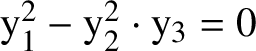 $\mathrm {y}_1^2-\mathrm {y}_2^2\cdot \mathrm {y}_3=0$
and the arc
$\mathrm {y}_1^2-\mathrm {y}_2^2\cdot \mathrm {y}_3=0$
and the arc
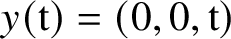 $y(\mathrm {t})=(0,0,\mathrm {t})$
. It is entirely contained in the singular locus of X, which is the
$y(\mathrm {t})=(0,0,\mathrm {t})$
. It is entirely contained in the singular locus of X, which is the
 $\mathrm {y}_3$
-axis. Let
$\mathrm {y}_3$
-axis. Let
 $\widetilde y(\mathrm {t})=(a(\mathrm {t}), b(\mathrm {t}), \mathrm {t}+c(\mathrm {t}))$
be a deformation of
$\widetilde y(\mathrm {t})=(a(\mathrm {t}), b(\mathrm {t}), \mathrm {t}+c(\mathrm {t}))$
be a deformation of
 $y(\mathrm {t})$
, with
$y(\mathrm {t})$
, with
 $a(0)=b(0)=0$
and
$a(0)=b(0)=0$
and
 $c(\mathrm {t})$
of order at least
$c(\mathrm {t})$
of order at least
 $2$
in
$2$
in
 $\mathrm {t}$
. Substitution in the defining equation gives
$\mathrm {t}$
. Substitution in the defining equation gives
 $$ \begin{align*} a^2(\mathrm{t})-b^2(\mathrm{t})\cdot (\mathrm{t}+c(\mathrm{t}))=0, \end{align*} $$
which has, by comparison of orders, the only solution
 $a(\mathrm {t})=b(\mathrm {t})=0$
, and
$a(\mathrm {t})=b(\mathrm {t})=0$
, and
 $c(\mathrm {t})\in \mathrm {t}^2\cdot \mathbf {k}[[\mathrm {t}]]$
arbitrary. Therefore, any deformation of
$c(\mathrm {t})\in \mathrm {t}^2\cdot \mathbf {k}[[\mathrm {t}]]$
arbitrary. Therefore, any deformation of
 $y(\mathrm {t})$
of this type already lies in the arc space
$y(\mathrm {t})$
of this type already lies in the arc space
 $(\mathrm {Sing}\, X)_{\infty }$
of the singular locus of X.
$(\mathrm {Sing}\, X)_{\infty }$
of the singular locus of X.
Outline of the proof of the structure theorem. We briefly describe how the stratification of the variety
 ${\mathcal Y}$
and the factorisations of the strata
${\mathcal Y}$
and the factorisations of the strata
 ${\mathcal Y}_{jd}$
in Theorem 1.4 are obtained.Footnote
13
Instead of proving directly that the strata
${\mathcal Y}_{jd}$
in Theorem 1.4 are obtained.Footnote
13
Instead of proving directly that the strata
 ${\mathcal Y}_{jd}$
are isomorphic to Cartesian products
${\mathcal Y}_{jd}$
are isomorphic to Cartesian products
 ${\mathcal Z}_{jd}\times \mathcal A_{\circ }^{s}$
, we rather work with the defining system of equations
${\mathcal Z}_{jd}\times \mathcal A_{\circ }^{s}$
, we rather work with the defining system of equations
 $f(\mathrm {t},\mathrm {y}(\mathrm {t}))=0$
. We will show that such a system of equations can be linearised locally after a suitable stratification of the ambient space
$f(\mathrm {t},\mathrm {y}(\mathrm {t}))=0$
. We will show that such a system of equations can be linearised locally after a suitable stratification of the ambient space
 $\mathcal A_{\circ }^m$
by a suitable textile isomorphism – but this is only possible up to a finite-dimensional part. From this it will then be relatively easy to deduce that the zeroset
$\mathcal A_{\circ }^m$
by a suitable textile isomorphism – but this is only possible up to a finite-dimensional part. From this it will then be relatively easy to deduce that the zeroset
 ${\mathcal Y}$
has the required Cartesian product structure on each stratum. Let us give some more details of how the linearisation works.
${\mathcal Y}$
has the required Cartesian product structure on each stratum. Let us give some more details of how the linearisation works.
Define, for
 $d\in {\mathbb N}$
and a suitably chosen minor g of the relative Jacobian matrix
$d\in {\mathbb N}$
and a suitably chosen minor g of the relative Jacobian matrix
 ${\partial }_{\mathrm {y}} f=({\partial }_{\mathrm {y}_i}f_j)$
of f with respect to
${\partial }_{\mathrm {y}} f=({\partial }_{\mathrm {y}_i}f_j)$
of f with respect to
 $\mathrm {y}$
, subsets
$\mathrm {y}$
, subsets
 ${\mathcal S}_d={\mathcal S}_d(g)$
of
${\mathcal S}_d={\mathcal S}_d(g)$
of
 $\mathcal A_{\circ }^m$
as the sets of vectors
$\mathcal A_{\circ }^m$
as the sets of vectors
 $y\in \mathcal A_{\circ }^m$
for which g has nonzero evaluation
$y\in \mathcal A_{\circ }^m$
for which g has nonzero evaluation
 $g(y)$
of order d as a power series in
$g(y)$
of order d as a power series in
 $\mathrm {t}$
. The sets
$\mathrm {t}$
. The sets
 ${\mathcal S}_d$
are textile cofinite and textile locally closed in
${\mathcal S}_d$
are textile cofinite and textile locally closed in
 $\mathcal A_{\circ }^m$
in the sense that the condition
$\mathcal A_{\circ }^m$
in the sense that the condition
 $\mathrm {ord}\,g(y)=d$
carries only on the (finitely many) coefficients
$\mathrm {ord}\,g(y)=d$
carries only on the (finitely many) coefficients
 $y_{ij}$
,
$y_{ij}$
,
 $1\leq i \leq m$
,
$1\leq i \leq m$
,
 $j\leq d$
, of vectors
$j\leq d$
, of vectors
 $y\in \mathcal A_{\circ }^m$
. It is not difficult to see that the order condition is given by (finitely many) polynomial equalities
$y\in \mathcal A_{\circ }^m$
. It is not difficult to see that the order condition is given by (finitely many) polynomial equalities
 $=$
and inequalities
$=$
and inequalities
 $\neq $
on these coefficients.Footnote
14
$\neq $
on these coefficients.Footnote
14
On each stratum
 ${\mathcal S}_d$
, the vectors
${\mathcal S}_d$
, the vectors
 $y\in {\mathcal S}_d$
will be decomposed uniquely by Weierstrass division into
$y\in {\mathcal S}_d$
will be decomposed uniquely by Weierstrass division into
 $y=z+v$
where z is a polynomial vector of degree
$y=z+v$
where z is a polynomial vector of degree
 $\leq d$
in
$\leq d$
in
 $\mathrm {t}$
and v is a power series vector whose components all have order
$\mathrm {t}$
and v is a power series vector whose components all have order
 $>d$
in
$>d$
in
 $\mathrm {t}$
. As y varies in the stratum
$\mathrm {t}$
. As y varies in the stratum
 ${\mathcal S}_d$
, the first summand z will vary in a finite-dimensional space. This type of decomposition is a standard technique in Artin approximation and in various results on arc spaces. It will allow us to show that
${\mathcal S}_d$
, the first summand z will vary in a finite-dimensional space. This type of decomposition is a standard technique in Artin approximation and in various results on arc spaces. It will allow us to show that
 ${f_{\infty }}(y)={f_{\infty }}(z+v)$
can be linearised with respect to v by an isomorphism
${f_{\infty }}(y)={f_{\infty }}(z+v)$
can be linearised with respect to v by an isomorphism
 $\chi _d$
of
$\chi _d$
of
 ${\mathcal S}_d$
. The precise statement is as follows (see Theorem 5.4 for more details).
${\mathcal S}_d$
. The precise statement is as follows (see Theorem 5.4 for more details).
Theorem 1.9. Linearisation of arquile maps
Let be given an arquile map
 ${f_{\infty }}:\mathcal A_{\circ }^m\rightarrow {\mathcal A}^k,\, y(\mathrm {t})\rightarrow f(\mathrm {t},y(\mathrm {t}))$
induced by the substitution of the
${f_{\infty }}:\mathcal A_{\circ }^m\rightarrow {\mathcal A}^k,\, y(\mathrm {t})\rightarrow f(\mathrm {t},y(\mathrm {t}))$
induced by the substitution of the
 $\mathrm {y}$
-variables by a vector
$\mathrm {y}$
-variables by a vector
 $y(\mathrm {t})$
of power series in a given power series vector
$y(\mathrm {t})$
of power series in a given power series vector
 $f\in {\mathcal B}^k$
. Assume that
$f\in {\mathcal B}^k$
. Assume that
 $k\leq m$
and let g be a
$k\leq m$
and let g be a
 $(k\times k)$
-minor of the relative Jacobian matrix
$(k\times k)$
-minor of the relative Jacobian matrix
 ${\partial }_{\mathrm {y}} f$
of f. Set
${\partial }_{\mathrm {y}} f$
of f. Set
 ${\mathcal S}_d= \{y\in \mathcal A_{\circ }^m,\, g(y)\neq 0$
,
${\mathcal S}_d= \{y\in \mathcal A_{\circ }^m,\, g(y)\neq 0$
,
 $\mathrm {ord}\, g(y)=d\}$
.
$\mathrm {ord}\, g(y)=d\}$
.
There then exists, for each
 $d\in {\mathbb N}$
, a textile isomorphism
$d\in {\mathbb N}$
, a textile isomorphism
 $\chi _d:{\mathcal Z}_d\times {\mathcal V}_d\,\,\smash {\mathop {\longrightarrow }\limits ^{\cong }}\,\, {\mathcal S}_d$
over
$\chi _d:{\mathcal Z}_d\times {\mathcal V}_d\,\,\smash {\mathop {\longrightarrow }\limits ^{\cong }}\,\, {\mathcal S}_d$
over
 ${\mathcal Z}_d$
from the Cartesian product of the quasi-affine algebraic variety
${\mathcal Z}_d$
from the Cartesian product of the quasi-affine algebraic variety
 ${\mathcal Z}_d=\{z\in \mathbf {k}_{\circ }[\mathrm {t}]_{\leq d}^m,\, \mathrm {ord}\, g(z)=d\}$
with the
${\mathcal Z}_d=\{z\in \mathbf {k}_{\circ }[\mathrm {t}]_{\leq d}^m,\, \mathrm {ord}\, g(z)=d\}$
with the
 $\mathcal A_{\circ }$
-module
$\mathcal A_{\circ }$
-module
 ${\mathcal V}_d=\langle \mathrm {t}\rangle ^d\cdot \mathcal A_{\circ }^m$
such that the composition
${\mathcal V}_d=\langle \mathrm {t}\rangle ^d\cdot \mathcal A_{\circ }^m$
such that the composition
 $$ \begin{align*} {f_{\infty}}\circ\chi_d:{\mathcal Z}_d\times{\mathcal V}_d\,\,\smash{\mathop{\longrightarrow}\limits^{\cong}}\,\, {\mathcal S}_d\,\,\smash{\mathop{\longrightarrow}\limits^{f_{\infty}}}\,\, {\mathcal A}^k \end{align*} $$
is linear in the second component and of the form
 $$ \begin{align*} ({f_{\infty}}\circ\chi_d)(z,v) = f(z)+{\partial}_{\mathrm{y}} f(z)\cdot v. \end{align*} $$
This statement can be rephrased by saying that
 ${f_{\infty }}$
is linearised on each stratum
${f_{\infty }}$
is linearised on each stratum
 ${\mathcal S}_d$
up to a finite-dimensional summand by an isomorphism of the source space. If the minor g is identically zero on
${\mathcal S}_d$
up to a finite-dimensional summand by an isomorphism of the source space. If the minor g is identically zero on
 $\mathcal A_{\circ }^m$
, all sets
$\mathcal A_{\circ }^m$
, all sets
 ${\mathcal S}_d$
are empty and the statement is vacuous. So the interesting case occurs when g is different from zero. The assumption that g stems from a submatrix of
${\mathcal S}_d$
are empty and the statement is vacuous. So the interesting case occurs when g is different from zero. The assumption that g stems from a submatrix of
 ${\partial }_{\mathrm {y}} f$
of size k (and hence the number k of components of f is less than or equal to the number m of
${\partial }_{\mathrm {y}} f$
of size k (and hence the number k of components of f is less than or equal to the number m of
 $\mathrm {y}$
-variables) is essential for the linearisation to work. A substantial part of the proof of Theorem 1.4 is dedicated to establishing this assumption on the sets of a suitable partition of
$\mathrm {y}$
-variables) is essential for the linearisation to work. A substantial part of the proof of Theorem 1.4 is dedicated to establishing this assumption on the sets of a suitable partition of
 ${\mathcal Y}(f)$
.
${\mathcal Y}(f)$
.
The construction of the linearisation of
 ${f_{\infty }}$
is the main technical ingredient of the article. It will be given explicitly by describing the isomorphism
${f_{\infty }}$
is the main technical ingredient of the article. It will be given explicitly by describing the isomorphism
 $\chi _d$
as a composition of a
$\chi _d$
as a composition of a
 $\mathbf {k}$
-linear isomorphism given by the Weierstrass division and an invertible arquile map. Here, the polynomial vector z plays the role of a parameter, and
$\mathbf {k}$
-linear isomorphism given by the Weierstrass division and an invertible arquile map. Here, the polynomial vector z plays the role of a parameter, and
 ${f_{\infty }}\circ \chi _d$
will depend in an arquile way on z (i.e., is a power series in z), whereas it is linear in v. The isomorphism
${f_{\infty }}\circ \chi _d$
will depend in an arquile way on z (i.e., is a power series in z), whereas it is linear in v. The isomorphism
 $\chi _d$
is textile in both v and z. Once the linearisation of
$\chi _d$
is textile in both v and z. Once the linearisation of
 ${f_{\infty }}$
with respect to v is achieved, a quite direct argument establishes the Cartesian factorisation of the stratum
${f_{\infty }}$
with respect to v is achieved, a quite direct argument establishes the Cartesian factorisation of the stratum
 ${\mathcal Y}_d={\mathcal Y}(f)\cap {\mathcal S}_d$
of
${\mathcal Y}_d={\mathcal Y}(f)\cap {\mathcal S}_d$
of
 ${\mathcal Y}(f)$
as described in Theorem 1.4.
${\mathcal Y}(f)$
as described in Theorem 1.4.
For arbitrary vectors f, the zeroset
 ${\mathcal Y}(f)$
has first to be decomposed into the arq.regular and arq.singular loci. On the first, there exists a covering by arquile open subsets for which linearisation works. On the second, one iterates the decomposition into the arq.regular and arq.singular loci and then argues by Noetherian induction to construct the required partition. Combining all strata of all subsets obtained in this way then yields the required partition
${\mathcal Y}(f)$
has first to be decomposed into the arq.regular and arq.singular loci. On the first, there exists a covering by arquile open subsets for which linearisation works. On the second, one iterates the decomposition into the arq.regular and arq.singular loci and then argues by Noetherian induction to construct the required partition. Combining all strata of all subsets obtained in this way then yields the required partition
 ${\mathcal Y}=\bigcup {\mathcal Y}_i$
together with the individual Cartesian product factorisations as described in the structure theorem 1.4.
${\mathcal Y}=\bigcup {\mathcal Y}_i$
together with the individual Cartesian product factorisations as described in the structure theorem 1.4.
Organisation of the article. After a compilation of definitions in Section 2, we recall the Weierstrass division theorem in Section 3 and adapt the statement to our purposes. This can be skipped on first reading, as well as the subsequent Section 4 on division modules. The main constructions appear in Section 5, where the linearisation theorem for arquile maps between power series spaces is formulated and proven. This is the central part of the article. The proof is elementary but a bit tricky. This result is then exploited in Sections 6, 7 and 9 to establish the various factorisation theorems. The intermediate Section 8 constructs the appropriate covering and stratification of an arquile variety. In Section 10 we illustrate our techniques in an explicit example. Section 11 discusses the analytic triviality of arquile varieties; that is, the appearance of a smooth factor in the formal neighbourhood of a point. A list of symbols can be found after the references.
2 Arquile varieties
In this section, we collect the basic material on arquile varietes needed in later sections. To ease the orientation of the reader, some overlap with Section 1 is admitted.
Our ground field
 $\mathbf {k}$
will be a perfect field of arbitrary characteristic. It will be assumed to be equipped with a valuation
$\mathbf {k}$
will be a perfect field of arbitrary characteristic. It will be assumed to be equipped with a valuation
 $\vert -\vert :\mathbf {k}\rightarrow \mathbb R$
whenever we talk about convergent power series. To ease notation we often suppress the dependence of power series
$\vert -\vert :\mathbf {k}\rightarrow \mathbb R$
whenever we talk about convergent power series. To ease notation we often suppress the dependence of power series
 $y=y(\mathrm {t})$
on the variable
$y=y(\mathrm {t})$
on the variable
 $\mathrm {t}$
. Vectors
$\mathrm {t}$
. Vectors
 $f=f(\mathrm {t},\mathrm {y})$
will be written as columns of length k, vectors of variables
$f=f(\mathrm {t},\mathrm {y})$
will be written as columns of length k, vectors of variables
 $\mathrm {y}$
and
$\mathrm {y}$
and
 $\mathrm {z}$
and of power series
$\mathrm {z}$
and of power series
 $y=y(\mathrm {t})$
as rows of length m. Accordingly, the relative Jacobian matrix
$y=y(\mathrm {t})$
as rows of length m. Accordingly, the relative Jacobian matrix
 ${\partial }_{\mathrm {y}} f$
of f will be a
${\partial }_{\mathrm {y}} f$
of f will be a
 $(k\times m)$
-matrix.
$(k\times m)$
-matrix.
Spaces of power series. We denote by
 $\mathcal A_{\circ }$
the ring of formal, respectively convergent or algebraic, power series
$\mathcal A_{\circ }$
the ring of formal, respectively convergent or algebraic, power series
 $y(\mathrm {t})$
in a single variable
$y(\mathrm {t})$
in a single variable
 $\mathrm {t}$
over
$\mathrm {t}$
over
 $\mathbf {k}$
and without constant term,
$\mathbf {k}$
and without constant term,
 $y(0)=0$
.Footnote
15
This is a commutative ring without one element
$y(0)=0$
.Footnote
15
This is a commutative ring without one element
 $1$
. For
$1$
. For
 $m\in {\mathbb N}$
we will consider vectors
$m\in {\mathbb N}$
we will consider vectors
 $y=(y_1,\ldots ,y_m)\in \mathcal A_{\circ }^m$
of power series without constant terms and call accordingly
$y=(y_1,\ldots ,y_m)\in \mathcal A_{\circ }^m$
of power series without constant terms and call accordingly
 $y_{ij}=(y_{ij},\, 1\leq i \leq m,\, j\geq 1)\in (\mathbf {k}^{{\mathbb N}_{>0}})^m$
their coefficient vector. We will interpret
$y_{ij}=(y_{ij},\, 1\leq i \leq m,\, j\geq 1)\in (\mathbf {k}^{{\mathbb N}_{>0}})^m$
their coefficient vector. We will interpret
 $\mathcal A_{\circ }^m$
as an infinite-dimensional affine space over
$\mathcal A_{\circ }^m$
as an infinite-dimensional affine space over
 $\mathbf {k}$
. In the setting of formal power series, its ‘coordinate ring’ is the polynomial ring
$\mathbf {k}$
. In the setting of formal power series, its ‘coordinate ring’ is the polynomial ring
 $\mathbf {k}[y_{m,\infty }]=\mathbf {k}[\mathrm {y}_{ij},\, 1\leq i \leq m,\, j\geq 1]$
in countably many variables.
$\mathbf {k}[y_{m,\infty }]=\mathbf {k}[\mathrm {y}_{ij},\, 1\leq i \leq m,\, j\geq 1]$
in countably many variables.
Arquile maps. For variables
 $\mathrm {y}=(\mathrm {y}_1,\ldots ,\mathrm {y}_m)$
, let
$\mathrm {y}=(\mathrm {y}_1,\ldots ,\mathrm {y}_m)$
, let
 ${\mathcal B}$
denote one of the rings
${\mathcal B}$
denote one of the rings
 $\mathbf {k}[[\mathrm {t},\mathrm {y}]]$
,
$\mathbf {k}[[\mathrm {t},\mathrm {y}]]$
,
 $\mathbf {k}\{\mathrm {t},\mathrm {y}\}$
or
$\mathbf {k}\{\mathrm {t},\mathrm {y}\}$
or
 $\mathbf {k}\langle \mathrm {t},\mathrm {y}\rangle $
of power series in
$\mathbf {k}\langle \mathrm {t},\mathrm {y}\rangle $
of power series in
 $\mathrm {t}$
and
$\mathrm {t}$
and
 $\mathrm {y}$
. If f is in
$\mathrm {y}$
. If f is in
 ${\mathcal B}$
and
${\mathcal B}$
and
 $y=y(\mathrm {t})\in \mathcal A_{\circ }^m$
, we may replace in f the
$y=y(\mathrm {t})\in \mathcal A_{\circ }^m$
, we may replace in f the
 $\mathrm {y}$
-variables by the vector
$\mathrm {y}$
-variables by the vector
 $y(t)$
, which we abbreviate by
$y(t)$
, which we abbreviate by
 $f(y)=f(\mathrm {t},y(\mathrm {t}))$
. Here and in the sequel, the qualities of
$f(y)=f(\mathrm {t},y(\mathrm {t}))$
. Here and in the sequel, the qualities of
 $\mathcal A_{\circ }$
and
$\mathcal A_{\circ }$
and
 ${\mathcal B}$
(formal, convergent or algebraic) are tacitly accorded. Every vector
${\mathcal B}$
(formal, convergent or algebraic) are tacitly accorded. Every vector
 $f\in {\mathcal B}^k$
induces an arquile map
$f\in {\mathcal B}^k$
induces an arquile map
 $$ \begin{align*} \begin{array}{rcl} {f_{\infty}}: \mathcal A_{\circ}^m& \longrightarrow & {\mathcal A}^k,\\ y & \longrightarrow & f(y) \end{array} \end{align*} $$
by evaluation at y. If f is a linear polynomial in
 $y_1,\ldots ,y_m$
with coefficients in
$y_1,\ldots ,y_m$
with coefficients in
 $\mathcal A_{\circ }$
, the induced map
$\mathcal A_{\circ }$
, the induced map
 ${f_{\infty }}$
is
${f_{\infty }}$
is
 $\mathcal A_{\circ }$
-linear. If
$\mathcal A_{\circ }$
-linear. If
 ${\mathcal S}$
is a subset of
${\mathcal S}$
is a subset of
 $\mathcal A_{\circ }^m$
, we may restrict
$\mathcal A_{\circ }^m$
, we may restrict
 ${f_{\infty }}$
to
${f_{\infty }}$
to
 ${\mathcal S}$
to get an arquile map
${\mathcal S}$
to get an arquile map
 ${f_{\infty }} :{\mathcal S}\rightarrow {\mathcal A}^k$
.
${f_{\infty }} :{\mathcal S}\rightarrow {\mathcal A}^k$
.
Theorem 2.1. Inverse function theorem
For any vector
 $p(\mathrm {t},\mathrm {y})\in {\mathcal B}^m$
whose components are all of order at least
$p(\mathrm {t},\mathrm {y})\in {\mathcal B}^m$
whose components are all of order at least
 $2$
in
$2$
in
 $\mathrm {t},\mathrm {y}$
, the arquile map
$\mathrm {t},\mathrm {y}$
, the arquile map
 $$ \begin{align*} \begin{array}{rcl} \varphi: \mathcal A_{\circ}^m& \longrightarrow & \mathcal A_{\circ}^m,\\ y & \longrightarrow & y+p(y), \end{array} \end{align*} $$
is an arquile isomorphism.
Remark 2.2. In contrast to the finite-dimensional setting, and due to the fact that we restrict to power series without constant term, the map
 $\varphi $
is a global arquile isomorphism.
$\varphi $
is a global arquile isomorphism.
Proof. Set
 $u= \mathrm {y}+p(\mathrm {t},\mathrm {y})\in {\mathcal B}^m$
so that
$u= \mathrm {y}+p(\mathrm {t},\mathrm {y})\in {\mathcal B}^m$
so that
 $\varphi =u_{\infty }$
. We have
$\varphi =u_{\infty }$
. We have
 $u(0,0)=0$
, and the relative Jacobian matrix
$u(0,0)=0$
, and the relative Jacobian matrix
 ${\partial }_{\mathrm {y}}u(0,0)$
is invertible by the assumption on p. Let
${\partial }_{\mathrm {y}}u(0,0)$
is invertible by the assumption on p. Let
 $v\in {\mathcal B}^m$
be the unique vector with
$v\in {\mathcal B}^m$
be the unique vector with
 $v(0,0)=0$
and
$v(0,0)=0$
and
 $u(\mathrm {x},v(\mathrm {x},\mathrm {y}))=\mathrm {y}$
as given by the finite-dimensional implicit function theorem in the formal, convergent and algebraic context (in the last case, it is equivalent to Hensel’s lemma; see [Reference NagataNag]). Then v defines a globally defined arquile map
$u(\mathrm {x},v(\mathrm {x},\mathrm {y}))=\mathrm {y}$
as given by the finite-dimensional implicit function theorem in the formal, convergent and algebraic context (in the last case, it is equivalent to Hensel’s lemma; see [Reference NagataNag]). Then v defines a globally defined arquile map
 $\psi =v_{\infty }:\mathcal A_{\circ }^m \rightarrow \mathcal A_{\circ }^m$
via
$\psi =v_{\infty }:\mathcal A_{\circ }^m \rightarrow \mathcal A_{\circ }^m$
via
 $y\rightarrow v(y)$
. Clearly,
$y\rightarrow v(y)$
. Clearly,
 $\psi \circ \varphi $
is the identity map on
$\psi \circ \varphi $
is the identity map on
 $\mathcal A_{\circ }^m$
.
$\mathcal A_{\circ }^m$
.
Arquile varieties. Every ideal I of
 ${\mathcal B}$
defines a subset
${\mathcal B}$
defines a subset
 ${\mathcal Y}$
of
${\mathcal Y}$
of
 $\mathcal A_{\circ }^m$
by
$\mathcal A_{\circ }^m$
by
 $$ \begin{align*} {\mathcal Y}={\mathcal Y}(I)=\{y\in\mathcal A_{\circ}^m,\, f(y)=0 \text{ for all } f\in I\}. \end{align*} $$
We call such sets arquile subvarieties of
 $\mathcal A_{\circ }^m$
, or simply arquile varieties. We also say that these sets are arquile closed in
$\mathcal A_{\circ }^m$
, or simply arquile varieties. We also say that these sets are arquile closed in
 $\mathcal A_{\circ }^m$
. They are the fibres
$\mathcal A_{\circ }^m$
. They are the fibres
 $f_{\infty }^{-1}(0)$
of arquile maps
$f_{\infty }^{-1}(0)$
of arquile maps
 $f_{\infty }:\mathcal A_{\circ }^m\rightarrow \mathcal A_{\circ }^k$
induced by a vector
$f_{\infty }:\mathcal A_{\circ }^m\rightarrow \mathcal A_{\circ }^k$
induced by a vector
 $f\in {\mathcal B}^k$
with
$f\in {\mathcal B}^k$
with
 $f(0)=0$
, where the components of f generate the ideal I in
$f(0)=0$
, where the components of f generate the ideal I in
 ${\mathcal B}$
. Note that arquile open subsets of
${\mathcal B}$
. Note that arquile open subsets of
 $\mathcal A_{\circ }^m$
are
$\mathcal A_{\circ }^m$
are
 $\mathrm {t}$
-adically open.
$\mathrm {t}$
-adically open.
Given two ideals I and J of
 ${\mathcal B}$
, we have
${\mathcal B}$
, we have
 ${\mathcal Y}(I\cap J)={\mathcal Y}(I)\cup {\mathcal Y}(J)$
and
${\mathcal Y}(I\cap J)={\mathcal Y}(I)\cup {\mathcal Y}(J)$
and
 ${\mathcal Y}(I+ J)={\mathcal Y}(I)\cap {\mathcal Y}(J)$
. It is clear that if
${\mathcal Y}(I+ J)={\mathcal Y}(I)\cap {\mathcal Y}(J)$
. It is clear that if
 $\sqrt I$
denotes the radical of I, then
$\sqrt I$
denotes the radical of I, then
 ${\mathcal Y}(I)={\mathcal Y}(\sqrt I)$
. So we may assume without loss of generality that arquile subvarieties
${\mathcal Y}(I)={\mathcal Y}(\sqrt I)$
. So we may assume without loss of generality that arquile subvarieties
 ${\mathcal Y}(I)$
are defined by radical ideals
${\mathcal Y}(I)$
are defined by radical ideals
 $I=\sqrt I$
.Footnote
16
For
$I=\sqrt I$
.Footnote
16
For
 ${\mathcal Y}$
an arbitrary subset of
${\mathcal Y}$
an arbitrary subset of
 $\mathcal A_{\circ }^m$
we define
$\mathcal A_{\circ }^m$
we define
 $$ \begin{align*} I_{{\mathcal Y}}=\{f\in{\mathcal B},\, f(y)=0 \text{ for all } y\in {\mathcal Y}\} \end{align*} $$
as the ideal of
 ${\mathcal B}$
of power series vanishing upon the substitution of the variables
${\mathcal B}$
of power series vanishing upon the substitution of the variables
 $\mathrm {y}$
by elements y of
$\mathrm {y}$
by elements y of
 ${\mathcal Y}$
. The ideal I is called saturated if I equals its saturation
${\mathcal Y}$
. The ideal I is called saturated if I equals its saturation
 $I_{{\mathcal Y}(I)}$
. The saturation of an arbitrary ideal I is always radical; for the converse in the convergent case, see Theorem 2.8.
$I_{{\mathcal Y}(I)}$
. The saturation of an arbitrary ideal I is always radical; for the converse in the convergent case, see Theorem 2.8.
Proposition 2.3. Let I be a saturated proper ideal of
 ${\mathcal B}$
, with irredundant prime decomposition
${\mathcal B}$
, with irredundant prime decomposition
 $I=I_1\cap \ldots \cap I_s$
. Then all
$I=I_1\cap \ldots \cap I_s$
. Then all
 $I_i$
are saturated, say
$I_i$
are saturated, say
 ${\mathcal Y}(I)={\mathcal Y}(I_1)\cup \ldots \cup {\mathcal Y}(I_s)$
with
${\mathcal Y}(I)={\mathcal Y}(I_1)\cup \ldots \cup {\mathcal Y}(I_s)$
with
 $I_i=I_{{\mathcal Y}(I_i)}$
, and
$I_i=I_{{\mathcal Y}(I_i)}$
, and
 ${\mathcal Y}(I_i)\neq \emptyset $
for all i.
${\mathcal Y}(I_i)\neq \emptyset $
for all i.
The arquile varieties
 ${\mathcal Y}(I_i)$
will be called the irreducible components of
${\mathcal Y}(I_i)$
will be called the irreducible components of
 ${\mathcal Y}$
(they are the irreducible components with respect to the arquile topology). While the prime components of a saturated ideal are again saturated, the saturation of a prime ideal need not be prime; cf. the example after the proof.
${\mathcal Y}$
(they are the irreducible components with respect to the arquile topology). While the prime components of a saturated ideal are again saturated, the saturation of a prime ideal need not be prime; cf. the example after the proof.
Proof. Suppose that
 $I_1$
is not saturated and hence properly contained in
$I_1$
is not saturated and hence properly contained in
 $I_{{\mathcal Y}(I_1)}$
, and let
$I_{{\mathcal Y}(I_1)}$
, and let
 $I_{1,1},\dots , I_{1,r}$
be an irredundant prime decomposition of
$I_{1,1},\dots , I_{1,r}$
be an irredundant prime decomposition of
 $I_{{\mathcal Y}(I_1)} = \bigcap _{j=1}^{r} I_{1,j}$
. Then
$I_{{\mathcal Y}(I_1)} = \bigcap _{j=1}^{r} I_{1,j}$
. Then
 $I \subset \bigcap _{j=1}^{r} I_{1,j} \cap I_{2} \cap \dots \cap I_{s}$
. Since the subvarieties of
$I \subset \bigcap _{j=1}^{r} I_{1,j} \cap I_{2} \cap \dots \cap I_{s}$
. Since the subvarieties of
 $\mathcal A_{\circ }^m$
associated to both ideals coincide and I is saturated, we obtain that
$\mathcal A_{\circ }^m$
associated to both ideals coincide and I is saturated, we obtain that
 $I = \bigcap _{j=1}^{r} I_{1,j} \cap I_{2} \cap \dots \cap I_{s}$
. This prime decomposition can be reduced to an irredundant one, and then
$I = \bigcap _{j=1}^{r} I_{1,j} \cap I_{2} \cap \dots \cap I_{s}$
. This prime decomposition can be reduced to an irredundant one, and then
 $I_{1}$
has to appear in the decomposition. The inequality
$I_{1}$
has to appear in the decomposition. The inequality
 $I_{i} \neq I_{j}$
for
$I_{i} \neq I_{j}$
for
 $i\neq j$
implies that
$i\neq j$
implies that
 $I_{1} = I_{1,l}$
for some l, which leads to
$I_{1} = I_{1,l}$
for some l, which leads to
 $I_{{\mathcal Y}(I_1)} \subset I_{1}$
, contradictory to
$I_{{\mathcal Y}(I_1)} \subset I_{1}$
, contradictory to
 $I_1\subsetneq I_{{\mathcal Y}(I_1)}$
. Hence, all associated primes of I are saturated. Finally, if
$I_1\subsetneq I_{{\mathcal Y}(I_1)}$
. Hence, all associated primes of I are saturated. Finally, if
 ${\mathcal Y}(I_{i})$
is empty, then
${\mathcal Y}(I_{i})$
is empty, then
 $I_{i} = I_{{\mathcal Y}(I_{i})} = {\mathcal B}$
, which is not possible since
$I_{i} = I_{{\mathcal Y}(I_{i})} = {\mathcal B}$
, which is not possible since
 $I_{i}$
is prime in
$I_{i}$
is prime in
 ${\mathcal B}$
and hence properly contained.
${\mathcal B}$
and hence properly contained.
Example 2.4. A theorem of Kolchin asserts that if
 $X\subset \mathbb A^m_{\mathbf {k}}$
is an irreducible algebraic variety over a field
$X\subset \mathbb A^m_{\mathbf {k}}$
is an irreducible algebraic variety over a field
 $\mathbf {k}$
of zero characteristic, the (global) arc space
$\mathbf {k}$
of zero characteristic, the (global) arc space
 $X_{\infty }$
consisting of arcs
$X_{\infty }$
consisting of arcs
 $y(\mathrm {t})$
on X with arbitrary starting point
$y(\mathrm {t})$
on X with arbitrary starting point
 $y(0) \in X$
is irreducible in the textile topology on
$y(0) \in X$
is irreducible in the textile topology on
 ${\mathcal A}^m=\mathbf {k}[[\mathrm {t}]]^m$
; see [Reference KolchinKo], Chapter IV, Proposition 10, or [Reference Ishii and KollárIK], Lemma 2.12.Footnote
17
${\mathcal A}^m=\mathbf {k}[[\mathrm {t}]]^m$
; see [Reference KolchinKo], Chapter IV, Proposition 10, or [Reference Ishii and KollárIK], Lemma 2.12.Footnote
17
In the case of convergent power series over
 $\mathbf {k}={\mathbb C}$
and if the ideal I is generated by series in
$\mathbf {k}={\mathbb C}$
and if the ideal I is generated by series in
 ${\mathbb C}\{\mathrm {y}\}$
not depending on
${\mathbb C}\{\mathrm {y}\}$
not depending on
 $\mathrm {t}$
, being radical implies that I is saturated, and
$\mathrm {t}$
, being radical implies that I is saturated, and
 ${\mathcal Y}(I)$
is irreducible if and only if I is prime; see Corollary 2.9. And if one starts with a polynomial ideal
${\mathcal Y}(I)$
is irreducible if and only if I is prime; see Corollary 2.9. And if one starts with a polynomial ideal
 $I \subset {\mathbb C}[\mathrm {y}]$
, then
$I \subset {\mathbb C}[\mathrm {y}]$
, then
 ${\mathcal Y}(I)$
is irreducible if and only if
${\mathcal Y}(I)$
is irreducible if and only if
 $I\cdot {\mathbb C}\{y\}$
is prime; see Corollary 2.10.
$I\cdot {\mathbb C}\{y\}$
is prime; see Corollary 2.10.
Textile maps. A map
 $\tau : U\subset \mathcal A_{\circ }^m\rightarrow {\mathcal A}^k$
is called textile if each coefficient of the power series expansion of the images
$\tau : U\subset \mathcal A_{\circ }^m\rightarrow {\mathcal A}^k$
is called textile if each coefficient of the power series expansion of the images
 $z(\mathrm {t})=\tau (y(\mathrm {t}))$
of vectors
$z(\mathrm {t})=\tau (y(\mathrm {t}))$
of vectors
 $y(\mathrm {t})=(y_1(\mathrm {t}),\ldots ,y_m(\mathrm {t}))\in \mathcal A_{\circ }^m$
depends polynomially on finitely many of the coefficients of the expansions of the vectors y: There exist, for
$y(\mathrm {t})=(y_1(\mathrm {t}),\ldots ,y_m(\mathrm {t}))\in \mathcal A_{\circ }^m$
depends polynomially on finitely many of the coefficients of the expansions of the vectors y: There exist, for
 $\ell \geq 0$
, polynomial vectors
$\ell \geq 0$
, polynomial vectors
 $F_{\ell }=(F_{1\ell },\ldots ,F_{k\ell })\in \mathbf {k}[\mathrm {y}_{m,\infty }]^k$
in countably many variables
$F_{\ell }=(F_{1\ell },\ldots ,F_{k\ell })\in \mathbf {k}[\mathrm {y}_{m,\infty }]^k$
in countably many variables
 $\mathrm {y}_{m,\infty }=\{\mathrm {y}_{ij},\, 1\leq i\leq m,\,j\geq 1\}$
, each of them only depending on finitely many of the variables, such that, writing
$\mathrm {y}_{m,\infty }=\{\mathrm {y}_{ij},\, 1\leq i\leq m,\,j\geq 1\}$
, each of them only depending on finitely many of the variables, such that, writing
 $y_j(\mathrm {t})=\sum _{i\geq 0} y_{ij}\cdot \mathrm {t}^i$
, we have
$y_j(\mathrm {t})=\sum _{i\geq 0} y_{ij}\cdot \mathrm {t}^i$
, we have
 $$ \begin{align*} z(\mathrm{t})=\tau(y(\mathrm{t}))=\sum_{\ell\geq 0} F_{\ell}(y_{m,\infty})\cdot \mathrm{t}^{\ell}. \end{align*} $$
Textile maps induce ring homomorphisms
 $$ \begin{align*} \alpha_{\tau}: \mathbf{k}[\mathrm{z}_{k,\infty}]\rightarrow \mathbf{k}[\mathrm{y}_{m,\infty}] \end{align*} $$
defined by
 $\alpha _{\tau }(\mathrm {z}_{n\ell })=F_{n\ell }(\mathrm {y}_{m,\infty })$
, for
$\alpha _{\tau }(\mathrm {z}_{n\ell })=F_{n\ell }(\mathrm {y}_{m,\infty })$
, for
 $n=1,\ldots ,k$
, and
$n=1,\ldots ,k$
, and
 $\ell \geq 0$
. Conversely, any
$\ell \geq 0$
. Conversely, any
 $\mathbf {k}$
-algebra homomorphism
$\mathbf {k}$
-algebra homomorphism
 $\alpha :\mathbf {k}[\mathrm {z}_{k,\infty }]\rightarrow \mathbf {k}[\mathrm {y}_{m,\infty }]$
induces, in the case of formal power series
$\alpha :\mathbf {k}[\mathrm {z}_{k,\infty }]\rightarrow \mathbf {k}[\mathrm {y}_{m,\infty }]$
induces, in the case of formal power series
 $\mathcal A_{\circ }=\mathbf {k}_{\circ }[[\mathrm {t}]]$
, a textile map
$\mathcal A_{\circ }=\mathbf {k}_{\circ }[[\mathrm {t}]]$
, a textile map
 $\tau _{\alpha }:\mathcal A_{\circ }^m\rightarrow {\mathcal A}^k$
.Footnote
18
$\tau _{\alpha }:\mathcal A_{\circ }^m\rightarrow {\mathcal A}^k$
.Footnote
18
Every arquile map
 ${f_{\infty }}: \mathcal A_{\circ }^m\rightarrow {\mathcal A}^k,\, y(\mathrm {t})\rightarrow f(\mathrm {t},y(\mathrm {t}))$
, associated to a vector
${f_{\infty }}: \mathcal A_{\circ }^m\rightarrow {\mathcal A}^k,\, y(\mathrm {t})\rightarrow f(\mathrm {t},y(\mathrm {t}))$
, associated to a vector
 $f\in {\mathcal B}^k$
is textile. Also, if
$f\in {\mathcal B}^k$
is textile. Also, if
 $y(\mathrm {t})=a(\mathrm {t})\cdot h(\mathrm {t})+z(\mathrm {t})$
denotes the componentwise division of
$y(\mathrm {t})=a(\mathrm {t})\cdot h(\mathrm {t})+z(\mathrm {t})$
denotes the componentwise division of
 $y\in \mathcal A_{\circ }^m$
by a power series
$y\in \mathcal A_{\circ }^m$
by a power series
 $h(\mathrm {t})$
of order d, the associated division maps
$h(\mathrm {t})$
of order d, the associated division maps
 $y\rightarrow v=a\cdot h(\mathrm {t})$
and
$y\rightarrow v=a\cdot h(\mathrm {t})$
and
 $y\rightarrow z$
are textile; see the section on Weierstrass division. These two types of maps together with their compositions and inversions will be the main instances of textile maps in this article. A textile isomorphism is a bijective textile map whose inverse is again textile. See [Reference Bruschek and HauserBH] for more information on textile maps.
$y\rightarrow z$
are textile; see the section on Weierstrass division. These two types of maps together with their compositions and inversions will be the main instances of textile maps in this article. A textile isomorphism is a bijective textile map whose inverse is again textile. See [Reference Bruschek and HauserBH] for more information on textile maps.
A map
 $\tau : {\mathcal U}\subset \mathcal A_{\circ }^m\rightarrow {\mathcal A}^k$
defined on a subset
$\tau : {\mathcal U}\subset \mathcal A_{\circ }^m\rightarrow {\mathcal A}^k$
defined on a subset
 ${\mathcal U}$
of
${\mathcal U}$
of
 $\mathcal A_{\circ }^m$
is called rationally textile if each coefficient of the power series expansion of the images
$\mathcal A_{\circ }^m$
is called rationally textile if each coefficient of the power series expansion of the images
 $\tau (y)$
of vectors
$\tau (y)$
of vectors
 $y\in \mathcal A_{\circ }^m$
is a rational function of finitely many of the coefficients of the expansions of the vectors y. The denominators of the rational functions are not allowed to vanish when evaluating them on the coefficients of vectors in
$y\in \mathcal A_{\circ }^m$
is a rational function of finitely many of the coefficients of the expansions of the vectors y. The denominators of the rational functions are not allowed to vanish when evaluating them on the coefficients of vectors in
 ${\mathcal U}$
. So a rationally textile map is defined on whole
${\mathcal U}$
. So a rationally textile map is defined on whole
 ${\mathcal U}$
. If
${\mathcal U}$
. If
 $y(\mathrm {t})=a(\mathrm {t})\cdot h(\mathrm {t}) +z(\mathrm {t})$
denotes the componentwise Weierstrass division of
$y(\mathrm {t})=a(\mathrm {t})\cdot h(\mathrm {t}) +z(\mathrm {t})$
denotes the componentwise Weierstrass division of
 $y\in \mathcal A_{\circ }^m$
by a series
$y\in \mathcal A_{\circ }^m$
by a series
 $h(\mathrm {t})$
of order d, the map
$h(\mathrm {t})$
of order d, the map
 $y\rightarrow a$
is rationally textile; cf. Theorem 3.1.
$y\rightarrow a$
is rationally textile; cf. Theorem 3.1.
Topologies. The affine space
 $\mathcal A_{\circ }^m$
over
$\mathcal A_{\circ }^m$
over
 $\mathcal A_{\circ }$
will be equipped with three topologies. The
$\mathcal A_{\circ }$
will be equipped with three topologies. The
 $\mathrm {t}$
-adic topology defined by the ideals
$\mathrm {t}$
-adic topology defined by the ideals
 $\langle \mathrm {t}\rangle ^d=\mathrm {t}^d\cdot \mathcal A_{\circ }$
of
$\langle \mathrm {t}\rangle ^d=\mathrm {t}^d\cdot \mathcal A_{\circ }$
of
 $\mathcal A_{\circ }$
, for
$\mathcal A_{\circ }$
, for
 $d\geq 0$
, as a basis of neighbourhoods of
$d\geq 0$
, as a basis of neighbourhoods of
 $0\in \mathcal A_{\circ }^m$
; the textile topology, whose closed sets are the zerosets of (possibly infinitely many) polynomial equations in the coefficient vectors of the expansions of vectors
$0\in \mathcal A_{\circ }^m$
; the textile topology, whose closed sets are the zerosets of (possibly infinitely many) polynomial equations in the coefficient vectors of the expansions of vectors
 $y\in \mathcal A_{\circ }^m$
; and the arquile topology, whose closed sets are the zerosets of arquile maps. All three topologies will appear in the sequel. The arquile topology is Noetherian since a descending chain of arquile varieties
$y\in \mathcal A_{\circ }^m$
; and the arquile topology, whose closed sets are the zerosets of arquile maps. All three topologies will appear in the sequel. The arquile topology is Noetherian since a descending chain of arquile varieties
 ${\mathcal Y}_1\supset {\mathcal Y}_2\supset \ldots $
corresponds to an increasing chain of saturated ideals
${\mathcal Y}_1\supset {\mathcal Y}_2\supset \ldots $
corresponds to an increasing chain of saturated ideals
 $I_1\subset I_2\subset \ldots $
of
$I_1\subset I_2\subset \ldots $
of
 ${\mathcal B}$
with
${\mathcal B}$
with
 ${\mathcal Y}_j={\mathcal Y}(I_j)$
.
${\mathcal Y}_j={\mathcal Y}(I_j)$
.
A subset of
 $\mathcal A_{\circ }^m$
is textile locally closed if it is the set-theoretic difference of two textile closed sets. Arquile subvarieties
$\mathcal A_{\circ }^m$
is textile locally closed if it is the set-theoretic difference of two textile closed sets. Arquile subvarieties
 ${\mathcal Y}(f)$
of
${\mathcal Y}(f)$
of
 $\mathcal A_{\circ }^m$
as defined above are textile closed and
$\mathcal A_{\circ }^m$
as defined above are textile closed and
 $\mathrm {t}$
-adically closed, since arquile maps
$\mathrm {t}$
-adically closed, since arquile maps
 ${f_{\infty }}$
are textile continuous and
${f_{\infty }}$
are textile continuous and
 $\mathrm {t}$
-adically continuous. Textile maps are textile continuous by definition. They are also
$\mathrm {t}$
-adically continuous. Textile maps are textile continuous by definition. They are also
 $\mathrm {t}$
-adically continuous, since each coefficient of a power series vector in the image depends only on finitely many coefficients of the power series vector in the source. In particular, textile isomorphisms are
$\mathrm {t}$
-adically continuous, since each coefficient of a power series vector in the image depends only on finitely many coefficients of the power series vector in the source. In particular, textile isomorphisms are
 $\mathrm {t}$
-adic homeomorphisms.
$\mathrm {t}$
-adic homeomorphisms.
Arquile maps
 ${f_{\infty }}:\mathcal A_{\circ }^m\rightarrow {\mathcal A}^k$
associated to vectors
${f_{\infty }}:\mathcal A_{\circ }^m\rightarrow {\mathcal A}^k$
associated to vectors
 $f\in {\mathcal B}^k$
map the
$f\in {\mathcal B}^k$
map the
 $\mathrm {t}$
-adic neighbourhood
$\mathrm {t}$
-adic neighbourhood
 $y+\langle \mathrm {t}\rangle ^c\cdot \mathcal A_{\circ }^m$
of a vector
$y+\langle \mathrm {t}\rangle ^c\cdot \mathcal A_{\circ }^m$
of a vector
 $y\in \mathcal A_{\circ }^m$
into the neighbourhood
$y\in \mathcal A_{\circ }^m$
into the neighbourhood
 ${f_{\infty }}(y)+\langle \mathrm {t}\rangle ^c\cdot {\mathcal A}^k$
. They are hence uniformly Lipschitz continuous with Lipschitz constant 1 with respect to the
${f_{\infty }}(y)+\langle \mathrm {t}\rangle ^c\cdot {\mathcal A}^k$
. They are hence uniformly Lipschitz continuous with Lipschitz constant 1 with respect to the
 $\mathrm {t}$
-adic metric on
$\mathrm {t}$
-adic metric on
 $\mathcal A_{\circ }$
. For division maps
$\mathcal A_{\circ }$
. For division maps
 $y\rightarrow v=a\cdot h(\mathrm {t})$
and
$y\rightarrow v=a\cdot h(\mathrm {t})$
and
 $y\rightarrow z$
sending
$y\rightarrow z$
sending
 $y\in \mathcal A_{\circ }^m$
to the summands
$y\in \mathcal A_{\circ }^m$
to the summands
 $y=v+z$
of the componentwise division
$y=v+z$
of the componentwise division
 $y=a\cdot h(\mathrm {t})+ z$
of y by a series
$y=a\cdot h(\mathrm {t})+ z$
of y by a series
 $h(\mathrm {t})$
of order d, the neighbourhood
$h(\mathrm {t})$
of order d, the neighbourhood
 $\langle \mathrm {t}\rangle ^c\cdot \mathcal A_{\circ }^m$
is mapped into
$\langle \mathrm {t}\rangle ^c\cdot \mathcal A_{\circ }^m$
is mapped into
 $\langle \mathrm {t}\rangle ^c\cdot \mathcal A_{\circ }^m$
. In contrast, the map
$\langle \mathrm {t}\rangle ^c\cdot \mathcal A_{\circ }^m$
. In contrast, the map
 $y\rightarrow a$
sending y to the quotient a maps
$y\rightarrow a$
sending y to the quotient a maps
 $\langle \mathrm {t}\rangle ^c\cdot \mathcal A_{\circ }^m$
only into
$\langle \mathrm {t}\rangle ^c\cdot \mathcal A_{\circ }^m$
only into
 $\langle \mathrm {t}\rangle ^{c-d}\cdot \mathcal A_{\circ }^m$
, for all
$\langle \mathrm {t}\rangle ^{c-d}\cdot \mathcal A_{\circ }^m$
, for all
 $c\geq d$
.
$c\geq d$
.
A textile closed subset
 ${\mathcal Z}$
of a subset
${\mathcal Z}$
of a subset
 ${\mathcal U}$
of
${\mathcal U}$
of
 $\mathcal A_{\circ }^m$
is cofinite in
$\mathcal A_{\circ }^m$
is cofinite in
 ${\mathcal U}$
if it can be defined (as a subset of
${\mathcal U}$
if it can be defined (as a subset of
 ${\mathcal U}$
) by finitely many polynomial equations in (finitely many) coefficients of the power series expansions of vectors of
${\mathcal U}$
) by finitely many polynomial equations in (finitely many) coefficients of the power series expansions of vectors of
 $\mathcal A_{\circ }^m$
. In the literature, such subsets are also known as cylindrical or generically stable. The analogous definition applies to textile locally closed subsets.
$\mathcal A_{\circ }^m$
. In the literature, such subsets are also known as cylindrical or generically stable. The analogous definition applies to textile locally closed subsets.
Singular locus. Let
 $y=y(\mathrm {t})\in \mathcal A_{\circ }^m$
be a given power series vector. We may associate to y the evaluation map
$y=y(\mathrm {t})\in \mathcal A_{\circ }^m$
be a given power series vector. We may associate to y the evaluation map
 $\varepsilon _y:{\mathcal B}\rightarrow \mathcal A_{\circ }$
sending the variable
$\varepsilon _y:{\mathcal B}\rightarrow \mathcal A_{\circ }$
sending the variable
 $\mathrm {y}$
to y. Its kernel
$\mathrm {y}$
to y. Its kernel
 $\mathrm {Ker}(\varepsilon _y)$
is a prime ideal of
$\mathrm {Ker}(\varepsilon _y)$
is a prime ideal of
 ${\mathcal B}$
which will be denoted by
${\mathcal B}$
which will be denoted by
 ${\mathcal P}_y$
,
${\mathcal P}_y$
,
 $$ \begin{align*} {\mathcal P}_y=\{f\in{\mathcal B},\, f(\mathrm{t},y(\mathrm{t}))=0\}. \\[-20pt] \end{align*} $$
It is called the ideal of relations between the components of y. This is, in contrast to the finite-dimensional situation of points in affine space
 $\mathbb A^m_{\mathbf {k}}$
over a field, never a maximal ideal. The map sending y to
$\mathbb A^m_{\mathbf {k}}$
over a field, never a maximal ideal. The map sending y to
 ${\mathcal P}_y$
is injective, since
${\mathcal P}_y$
is injective, since
 $y=y(\mathrm {t})$
can be reconstructed from the elements
$y=y(\mathrm {t})$
can be reconstructed from the elements
 $\mathrm {y}_i-y_i(\mathrm {t})$
of
$\mathrm {y}_i-y_i(\mathrm {t})$
of
 ${\mathcal P}_y$
.Footnote
19
We denote by
${\mathcal P}_y$
.Footnote
19
We denote by
 ${\mathcal B}_{{\mathcal P}_y}$
the localisation of
${\mathcal B}_{{\mathcal P}_y}$
the localisation of
 ${\mathcal B}$
at
${\mathcal B}$
at
 ${\mathcal P}_y$
.
${\mathcal P}_y$
.
Denote by
 $\overline {\mathcal P}_y$
the image of
$\overline {\mathcal P}_y$
the image of
 ${\mathcal P}_y$
in
${\mathcal P}_y$
in
 ${\mathcal B}/I$
. We then say that y is an arq.regular point of
${\mathcal B}/I$
. We then say that y is an arq.regular point of
 ${\mathcal Y}$
if the localisation
${\mathcal Y}$
if the localisation
 $({\mathcal B}/I)_{\overline {\mathcal P}_y}={\mathcal B}_{{\mathcal P}_y}/I\cdot {\mathcal B}_{{\mathcal P}_y}$
is a regular local ring. By the above, this is equivalent to saying that
$({\mathcal B}/I)_{\overline {\mathcal P}_y}={\mathcal B}_{{\mathcal P}_y}/I\cdot {\mathcal B}_{{\mathcal P}_y}$
is a regular local ring. By the above, this is equivalent to saying that
 $p_y$
is a regular point of the scheme Y. The locus of arq.regular points of
$p_y$
is a regular point of the scheme Y. The locus of arq.regular points of
 ${\mathcal Y}$
is denoted by
${\mathcal Y}$
is denoted by
 $\mathrm {Arq.Reg}({\mathcal Y})$
, and we set
$\mathrm {Arq.Reg}({\mathcal Y})$
, and we set
 $\mathrm {Arq.Sing}({\mathcal Y})={\mathcal Y}\setminus \mathrm {Arq.Reg}({\mathcal Y})$
, the arq.singular locus of
$\mathrm {Arq.Sing}({\mathcal Y})={\mathcal Y}\setminus \mathrm {Arq.Reg}({\mathcal Y})$
, the arq.singular locus of
 ${\mathcal Y}$
. If y is an arq.regular point of
${\mathcal Y}$
. If y is an arq.regular point of
 ${\mathcal Y}$
, it necessarily lies in a single irreducible component of
${\mathcal Y}$
, it necessarily lies in a single irreducible component of
 ${\mathcal Y}$
; cf. Proposition 2.3 and the theorem below. For local investigations at arq.regular points we may therefore assume that I is prime. The following version of the Jacobian criterion will be used repeatedly; cf. [Reference de Jong and PfisterdJP], Theorem 4.3.15, [Reference RuizRu], Proposition 4.3, and [Reference ZariskiZa], Theorem 7 and its corollary (recall that the ground field
${\mathcal Y}$
; cf. Proposition 2.3 and the theorem below. For local investigations at arq.regular points we may therefore assume that I is prime. The following version of the Jacobian criterion will be used repeatedly; cf. [Reference de Jong and PfisterdJP], Theorem 4.3.15, [Reference RuizRu], Proposition 4.3, and [Reference ZariskiZa], Theorem 7 and its corollary (recall that the ground field
 $\mathbf {k}$
is assumed to be perfect).
$\mathbf {k}$
is assumed to be perfect).
Proposition 2.5. Jacobian criterion
Let I be an ideal of
 ${\mathcal B}$
generated by elements
${\mathcal B}$
generated by elements
 $f_1,\ldots ,f_k$
, and let
$f_1,\ldots ,f_k$
, and let
 ${\mathcal P}$
be a prime ideal of
${\mathcal P}$
be a prime ideal of
 ${\mathcal B}$
containing I. Then
${\mathcal B}$
containing I. Then
 $({\mathcal B}/I)_{\overline {\mathcal P}}$
is a regular local ring if and only if the rank of the Jacobian matrix
$({\mathcal B}/I)_{\overline {\mathcal P}}$
is a regular local ring if and only if the rank of the Jacobian matrix
 ${\partial }_{\mathrm {t}\mathrm {y}} f$
of
${\partial }_{\mathrm {t}\mathrm {y}} f$
of
 $f=(f_1,\ldots ,f_k)$
modulo
$f=(f_1,\ldots ,f_k)$
modulo
 ${\mathcal P}$
equals the height of the ideal
${\mathcal P}$
equals the height of the ideal
 $I_{\mathcal P}=I\cdot {\mathcal B}_{{\mathcal P}}$
.
$I_{\mathcal P}=I\cdot {\mathcal B}_{{\mathcal P}}$
.
As a corollary, we get the following.
Theorem 2.6. Arq.regular and arq.singular locus
Let
 ${\mathcal Y}={\mathcal Y}(I)$
be an arquile variety in
${\mathcal Y}={\mathcal Y}(I)$
be an arquile variety in
 $\mathcal A_{\circ }^m$
defined by a saturated ideal I of
$\mathcal A_{\circ }^m$
defined by a saturated ideal I of
 ${\mathcal B}$
, and let
${\mathcal B}$
, and let
 $y=y(\mathrm {t})\in {\mathcal Y}$
be a point of
$y=y(\mathrm {t})\in {\mathcal Y}$
be a point of
 ${\mathcal Y}$
with prime ideal
${\mathcal Y}$
with prime ideal
 ${\mathcal P}_y$
. Denote by r the height of the ideal
${\mathcal P}_y$
. Denote by r the height of the ideal
 $I\cdot {\mathcal B}_{{\mathcal P}_y}$
.
$I\cdot {\mathcal B}_{{\mathcal P}_y}$
.
(a) The point y is an arq.regular point of
 ${\mathcal Y}$
, if and only if there exist elements
${\mathcal Y}$
, if and only if there exist elements
 $f_1,\ldots ,f_r$
in I and an
$f_1,\ldots ,f_r$
in I and an
 $(r\times r)$
-minor g of the relative Jacobian matrix
$(r\times r)$
-minor g of the relative Jacobian matrix
 ${\partial }_{\mathrm {y}}f$
of
${\partial }_{\mathrm {y}}f$
of
 $f=(f_1,\ldots ,f_r)$
with respect to
$f=(f_1,\ldots ,f_r)$
with respect to
 $\mathrm {y}$
which does not lie in
$\mathrm {y}$
which does not lie in
 ${\mathcal P}_y$
; that is, which satisfies
${\mathcal P}_y$
; that is, which satisfies
 $g(y)\neq 0$
.
$g(y)\neq 0$
.
(b) For every arq.regular point y of
 ${\mathcal Y}$
, one can choose
${\mathcal Y}$
, one can choose
 $f_1,\ldots ,f_r\in I$
and the minor
$f_1,\ldots ,f_r\in I$
and the minor
 $g\in {\mathcal B}\setminus {\mathcal P}_y$
as in assertion (a) such that
$g\in {\mathcal B}\setminus {\mathcal P}_y$
as in assertion (a) such that
 $y\in {\mathcal Y}(f)\setminus {\mathcal Y}(g)$
and
$y\in {\mathcal Y}(f)\setminus {\mathcal Y}(g)$
and
 $$ \begin{align*} {\mathcal Y}\setminus {\mathcal Y}(g) ={\mathcal Y}(f)\setminus {\mathcal Y}(g). \end{align*} $$
(c) The arq.regular locus
 $\mathrm {Arq.Reg}({\mathcal Y})$
of
$\mathrm {Arq.Reg}({\mathcal Y})$
of
 ${\mathcal Y}$
is covered by finitely many arquile open subsets of the form
${\mathcal Y}$
is covered by finitely many arquile open subsets of the form
 ${\mathcal Y}(f)\setminus {\mathcal Y}(g)$
as in assertion (b), for varying values r.
${\mathcal Y}(f)\setminus {\mathcal Y}(g)$
as in assertion (b), for varying values r.
(d) The intersections
 ${\mathcal Y}_i\cap {\mathcal Y}_j$
of irreducible components of
${\mathcal Y}_i\cap {\mathcal Y}_j$
of irreducible components of
 ${\mathcal Y}$
lie inside
${\mathcal Y}$
lie inside
 $\mathrm {Arq.Sing}({\mathcal Y})$
.
$\mathrm {Arq.Sing}({\mathcal Y})$
.
(e) The arq.singular locus
 $\mathrm {Arq.Sing}({\mathcal Y})$
is an arquile closed and proper subset of
$\mathrm {Arq.Sing}({\mathcal Y})$
is an arquile closed and proper subset of
 ${\mathcal Y}$
. The height of its defining ideal J in
${\mathcal Y}$
. The height of its defining ideal J in
 ${\mathcal B}$
is larger than the height of I.
${\mathcal B}$
is larger than the height of I.
Remarks 2.7. (a) Assertion (e) implies the finiteness of the filtration by the iterated arq.singular loci as claimed in assertion (a) of the structure theorem 1.4.
(b) If X is an affine algebraic variety over
 $\mathbf {k}$
with arc space
$\mathbf {k}$
with arc space
 $X_{\infty ,0}$
of arcs centred at
$X_{\infty ,0}$
of arcs centred at
 $0$
, the theorem shows that the arq.regular points of
$0$
, the theorem shows that the arq.regular points of
 $X_{\infty ,0}$
in the sense of arquile varieties correspond to arcs in X which are not entirely contained in its singular locus
$X_{\infty ,0}$
in the sense of arquile varieties correspond to arcs in X which are not entirely contained in its singular locus
 $\mathrm {Sing}\, X$
.
$\mathrm {Sing}\, X$
.
(c) The elements
 $f_1,\ldots ,f_r$
of assertion (b) form a regular sequence in
$f_1,\ldots ,f_r$
of assertion (b) form a regular sequence in
 ${\mathcal B}$
; that is, generate an ideal of height r. This follows from the Jacobian criterion.
${\mathcal B}$
; that is, generate an ideal of height r. This follows from the Jacobian criterion.
(d) It follows from assertion (a) that the arq.singular locus
 $\mathrm {Arq.Sing}({\mathcal Y})$
of an irreducible arquile variety
$\mathrm {Arq.Sing}({\mathcal Y})$
of an irreducible arquile variety
 ${\mathcal Y}$
is defined inside
${\mathcal Y}$
is defined inside
 ${\mathcal Y}$
by the (saturation of the) ideal generated by all
${\mathcal Y}$
by the (saturation of the) ideal generated by all
 $(r\times r)$
-minors of the relative Jacobian matrix
$(r\times r)$
-minors of the relative Jacobian matrix
 ${\partial }_{\mathrm {y}} f$
with respect to
${\partial }_{\mathrm {y}} f$
with respect to
 $\mathrm {y}$
of vectors
$\mathrm {y}$
of vectors
 $f=(f_1,\ldots ,f_r)$
of elements of I.
$f=(f_1,\ldots ,f_r)$
of elements of I.
Proof. Let us show (a). By the Jacobian criterion, there exist elements
 $f_1,\ldots ,f_r$
in I such that the entire Jacobian matrix
$f_1,\ldots ,f_r$
in I such that the entire Jacobian matrix
 ${\partial }_{\mathrm {t}\mathrm {y}}f$
of
${\partial }_{\mathrm {t}\mathrm {y}}f$
of
 $f=(f_1,\ldots ,f_r)$
has rank r modulo
$f=(f_1,\ldots ,f_r)$
has rank r modulo
 ${\mathcal P}_y$
. So there is an
${\mathcal P}_y$
. So there is an
 $(r\times r)$
-minor g of
$(r\times r)$
-minor g of
 ${\partial }_{\mathrm {t}\mathrm {y}}f$
which satisfies
${\partial }_{\mathrm {t}\mathrm {y}}f$
which satisfies
 $g(y)\neq 0$
. Deriving the equation
$g(y)\neq 0$
. Deriving the equation
 $f(\mathrm {t},y(\mathrm {t}))=0$
with respect to
$f(\mathrm {t},y(\mathrm {t}))=0$
with respect to
 $\mathrm {t}$
gives
$\mathrm {t}$
gives
 ${\partial }_{\mathrm {t}} f(y(\mathrm {t}))=-{\partial }_{\mathrm {y}} f(y(\mathrm {t}))\cdot {\partial }_{\mathrm {t}} y(\mathrm {t})$
. This shows that g can actually be chosen from the relative Jacobian matrix
${\partial }_{\mathrm {t}} f(y(\mathrm {t}))=-{\partial }_{\mathrm {y}} f(y(\mathrm {t}))\cdot {\partial }_{\mathrm {t}} y(\mathrm {t})$
. This shows that g can actually be chosen from the relative Jacobian matrix
 ${\partial }_{\mathrm {y}}f$
of f with respect to
${\partial }_{\mathrm {y}}f$
of f with respect to
 $\mathrm {y}$
. This proves the ‘only if’ part. The converse implication follows directly from the Jacobian criterion.
$\mathrm {y}$
. This proves the ‘only if’ part. The converse implication follows directly from the Jacobian criterion.
To prove (b), the strategy is as follows: select the irreducible component
 ${\mathcal Y}_1$
of
${\mathcal Y}_1$
of
 ${\mathcal Y}$
passing through y (anticipating here assertion (d)) and represent it as an irreducible component of a complete intersection defined by some elements
${\mathcal Y}$
passing through y (anticipating here assertion (d)) and represent it as an irreducible component of a complete intersection defined by some elements
 $f_1,\ldots ,f_r$
in
$f_1,\ldots ,f_r$
in
 ${\mathcal B}$
. From there, new elements
${\mathcal B}$
. From there, new elements
 $f^{\prime }_1,\ldots ,f^{\prime }_r$
will be constructed multiplying
$f^{\prime }_1,\ldots ,f^{\prime }_r$
will be constructed multiplying
 $f_1,\ldots ,f_r$
with the square
$f_1,\ldots ,f_r$
with the square
 $h^2$
of an element h of
$h^2$
of an element h of
 ${\mathcal B}$
whose zero-locus
${\mathcal B}$
whose zero-locus
 ${\mathcal Y}(h)$
contains all components of
${\mathcal Y}(h)$
contains all components of
 ${\mathcal Y}$
but
${\mathcal Y}$
but
 ${\mathcal Y}_1$
. The chosen minor
${\mathcal Y}_1$
. The chosen minor
 $g'$
of the Jacobian matrix of
$g'$
of the Jacobian matrix of
 $f'=(f^{\prime }_1,\ldots ,f^{\prime }_r)$
will then be a multiple of h from which we infer that
$f'=(f^{\prime }_1,\ldots ,f^{\prime }_r)$
will then be a multiple of h from which we infer that
 $f'$
and
$f'$
and
 $g'$
have the required properties.
$g'$
have the required properties.
Denote by
 $I_0\subset I$
the ideal of
$I_0\subset I$
the ideal of
 ${\mathcal B}$
generated by elements
${\mathcal B}$
generated by elements
 $f_1,\ldots ,f_r$
of I as indicated in assertion (a). The height of
$f_1,\ldots ,f_r$
of I as indicated in assertion (a). The height of
 $I_0\cdot {\mathcal B}_{{\mathcal P}_y}$
is at most r. By the choice of
$I_0\cdot {\mathcal B}_{{\mathcal P}_y}$
is at most r. By the choice of
 $f_1,\ldots f_r$
and the Jacobian criterion it is exactly r. This implies that y is an arq.regular point of
$f_1,\ldots f_r$
and the Jacobian criterion it is exactly r. This implies that y is an arq.regular point of
 ${\mathcal Y}(I_0)$
; that is, that the ring
${\mathcal Y}(I_0)$
; that is, that the ring
 $({\mathcal B}/I_0)_{\overline {\mathcal P}_y}={\mathcal B}_{{\mathcal P}_y}/I_0\cdot {\mathcal B}_{{\mathcal P}_y}$
is regular. In particular,
$({\mathcal B}/I_0)_{\overline {\mathcal P}_y}={\mathcal B}_{{\mathcal P}_y}/I_0\cdot {\mathcal B}_{{\mathcal P}_y}$
is regular. In particular,
 $I_0\cdot {\mathcal B}_{{\mathcal P}_y}$
is a prime ideal in
$I_0\cdot {\mathcal B}_{{\mathcal P}_y}$
is a prime ideal in
 ${\mathcal B}_{{\mathcal P}_y}$
. It is the localisation
${\mathcal B}_{{\mathcal P}_y}$
. It is the localisation
 $I_1\cdot {\mathcal B}_{{\mathcal P}_y}$
of a prime ideal
$I_1\cdot {\mathcal B}_{{\mathcal P}_y}$
of a prime ideal
 $I_1$
of
$I_1$
of
 ${\mathcal B}$
, the ideal defining the irreducible component
${\mathcal B}$
, the ideal defining the irreducible component
 ${\mathcal Y}_1$
of
${\mathcal Y}_1$
of
 ${\mathcal Y}$
passing through y. Therefore,
${\mathcal Y}$
passing through y. Therefore,
 $I_1$
is an associated prime of both I and
$I_1$
is an associated prime of both I and
 $I_0$
. We can write
$I_0$
. We can write
 $I_1=(I_0:h)$
as a colon ideal with some element
$I_1=(I_0:h)$
as a colon ideal with some element
 $h\in {\mathcal B}\setminus {\mathcal P}_y$
.
$h\in {\mathcal B}\setminus {\mathcal P}_y$
.
We now set
 $f_i'=h^2\cdot f_i$
, for
$f_i'=h^2\cdot f_i$
, for
 $i=1,\ldots ,r$
, and let
$i=1,\ldots ,r$
, and let
 $g'$
denote the minor of
$g'$
denote the minor of
 ${\partial }_{\mathrm {y}} f'$
defined by the same columns as those which were taken for g. Observe that h divides
${\partial }_{\mathrm {y}} f'$
defined by the same columns as those which were taken for g. Observe that h divides
 $g'$
. As
$g'$
. As
 $g(y)\neq 0$
and
$g(y)\neq 0$
and
 $h(y)\neq 0$
, we also have
$h(y)\neq 0$
, we also have
 $g'(y)\neq 0$
. Clearly,
$g'(y)\neq 0$
. Clearly,
 ${\mathcal Y}(h)\subset {\mathcal Y}(g')$
. Let
${\mathcal Y}(h)\subset {\mathcal Y}(g')$
. Let
 $I'=h^2\cdot I_0$
denote the ideal of
$I'=h^2\cdot I_0$
denote the ideal of
 ${\mathcal B}$
generated by
${\mathcal B}$
generated by
 $f_1',\ldots ,f_r'$
. As
$f_1',\ldots ,f_r'$
. As
 $I'\subset I$
, we have
$I'\subset I$
, we have
 ${\mathcal Y}(I)\subset {\mathcal Y}(I')$
. Conversely,
${\mathcal Y}(I)\subset {\mathcal Y}(I')$
. Conversely,
 $I_1=(I_0:h)$
implies that
$I_1=(I_0:h)$
implies that
 $h\cdot I_1\subset I_0$
and then
$h\cdot I_1\subset I_0$
and then
 $h^3\cdot I_1\subset I'$
. We get
$h^3\cdot I_1\subset I'$
. We get
 $$ \begin{align*} {\mathcal Y}(I')\subset{\mathcal Y}(h^3\cdot I_1)={\mathcal Y}(h)\cup{\mathcal Y}(I_1)\subset {\mathcal Y}(h)\cup{\mathcal Y}(I) \end{align*} $$
and thus
 $$ \begin{align*} {\mathcal Y}(I')\setminus{\mathcal Y}(h)\subset {\mathcal Y}(I)\setminus {\mathcal Y}(h), \end{align*} $$
from which, by
 $I'\subset I$
, follows the equality
$I'\subset I$
, follows the equality
 $$ \begin{align*} {\mathcal Y}(I)\setminus {\mathcal Y}(h)={\mathcal Y}(I')\setminus{\mathcal Y}(h). \end{align*} $$
The inclusion
 ${\mathcal Y}(h)\subset {\mathcal Y}(g')$
finally implies
${\mathcal Y}(h)\subset {\mathcal Y}(g')$
finally implies
 $$ \begin{align*} {\mathcal Y}(I')\setminus{\mathcal Y}(g')={\mathcal Y}(I)\setminus {\mathcal Y}(g'), \end{align*} $$
as was claimed in (b). Assertion (c) is obvious since the arquile topology is Noetherian.
To prove (d), let
 $I=I_1\cap \ldots \cap I_s$
be the irredundant prime decomposition of I. Order the ideals
$I=I_1\cap \ldots \cap I_s$
be the irredundant prime decomposition of I. Order the ideals
 $I_i$
such that y is contained in
$I_i$
such that y is contained in
 ${\mathcal Y}(I_i)$
for
${\mathcal Y}(I_i)$
for
 $i\leq t$
and not contained in
$i\leq t$
and not contained in
 ${\mathcal Y}(I_i)$
for
${\mathcal Y}(I_i)$
for
 $i>t$
, where
$i>t$
, where
 $1\leq t\leq s$
. Then
$1\leq t\leq s$
. Then
 $I\cdot {\mathcal B}_{{\mathcal P}_y}= I_1\cdot {\mathcal B}_{{\mathcal P}_y}\cap \ldots \cap I_t\cdot {\mathcal B}_{{\mathcal P}_y}$
. If y is contained in two irreducible components of
$I\cdot {\mathcal B}_{{\mathcal P}_y}= I_1\cdot {\mathcal B}_{{\mathcal P}_y}\cap \ldots \cap I_t\cdot {\mathcal B}_{{\mathcal P}_y}$
. If y is contained in two irreducible components of
 ${\mathcal Y}$
, then
${\mathcal Y}$
, then
 $I\cdot {\mathcal B}_{{\mathcal P}_y}$
is the intersection of at least two prime ideals and hence itself is not a prime ideal. Then
$I\cdot {\mathcal B}_{{\mathcal P}_y}$
is the intersection of at least two prime ideals and hence itself is not a prime ideal. Then
 ${\mathcal B}_{{\mathcal P}_y}/I\cdot {\mathcal B}_{{\mathcal P}_y}$
is not regular so that
${\mathcal B}_{{\mathcal P}_y}/I\cdot {\mathcal B}_{{\mathcal P}_y}$
is not regular so that
 $y\in \mathrm {Arq.Sing}({\mathcal Y})$
.
$y\in \mathrm {Arq.Sing}({\mathcal Y})$
.
We conclude with the proof of assertion (e). The arq.regular locus
 $\mathrm {Arq.Reg}({\mathcal Y})$
of
$\mathrm {Arq.Reg}({\mathcal Y})$
of
 ${\mathcal Y}$
is open by (c). For the remaining assertions, assume first that
${\mathcal Y}$
is open by (c). For the remaining assertions, assume first that
 ${\mathcal Y}$
is irreducible, say, that I is prime. Then
${\mathcal Y}$
is irreducible, say, that I is prime. Then
 $({\mathcal B}/I)_I$
is a field, in particular regular. By the Jacobian criterion there exist elements
$({\mathcal B}/I)_I$
is a field, in particular regular. By the Jacobian criterion there exist elements
 $f_1,\ldots ,f_r$
in I, where r is the height of
$f_1,\ldots ,f_r$
in I, where r is the height of
 $I\cdot {\mathcal B}_I$
, and a minor g of
$I\cdot {\mathcal B}_I$
, and a minor g of
 ${\partial }_{\mathrm {t}\mathrm {y}}f$
of
${\partial }_{\mathrm {t}\mathrm {y}}f$
of
 $f=(f_1,\ldots ,f_r)$
which is not contained in I. But I is saturated and
$f=(f_1,\ldots ,f_r)$
which is not contained in I. But I is saturated and
 ${\mathcal Y}={\mathcal Y}(I)$
is nonempty, so there is a point
${\mathcal Y}={\mathcal Y}(I)$
is nonempty, so there is a point
 $y\in {\mathcal Y}={\mathcal Y}(I)$
for which
$y\in {\mathcal Y}={\mathcal Y}(I)$
for which
 $g(y)\neq 0$
. This implies by the Jacobian criterion that
$g(y)\neq 0$
. This implies by the Jacobian criterion that
 $({\mathcal B}/I)_{\overline {\mathcal P}_y}$
is regular, so that y is an arq.regular point of
$({\mathcal B}/I)_{\overline {\mathcal P}_y}$
is regular, so that y is an arq.regular point of
 ${\mathcal Y}$
. Hence,
${\mathcal Y}$
. Hence,
 $\mathrm {Arq.Reg}({\mathcal Y})$
is nonempty and
$\mathrm {Arq.Reg}({\mathcal Y})$
is nonempty and
 $\mathrm {Arq.Sing}({\mathcal Y})$
is a proper subset of
$\mathrm {Arq.Sing}({\mathcal Y})$
is a proper subset of
 ${\mathcal Y}$
. Using the argument from the proof of assertion (a), we may choose for g a minor of the relative Jacobian matrix
${\mathcal Y}$
. Using the argument from the proof of assertion (a), we may choose for g a minor of the relative Jacobian matrix
 ${\partial }_{\mathrm {y}} f$
of f with respect to
${\partial }_{\mathrm {y}} f$
of f with respect to
 $\mathrm {y}$
. Let J denote the ideal of
$\mathrm {y}$
. Let J denote the ideal of
 ${\mathcal B}$
defining
${\mathcal B}$
defining
 $\mathrm {Arq.Sing}({\mathcal Y})$
. By definition,
$\mathrm {Arq.Sing}({\mathcal Y})$
. By definition,
 $I\subset J$
. But
$I\subset J$
. But
 $g\in J$
and
$g\in J$
and
 $g\not \in I$
, so that I is strictly contained in J. As I is prime, Krull’s principal ideal theorem ensures that the height of J is larger than the height of I. This establishes assertion (e) for prime ideals.
$g\not \in I$
, so that I is strictly contained in J. As I is prime, Krull’s principal ideal theorem ensures that the height of J is larger than the height of I. This establishes assertion (e) for prime ideals.
Let now I be arbitrary. It is easy to see that
 $\mathrm {Arq.Sing}({\mathcal Y})$
is composed of the union of the arq.singular loci
$\mathrm {Arq.Sing}({\mathcal Y})$
is composed of the union of the arq.singular loci
 $\mathrm {Arq.Sing}({\mathcal Y}_i)$
of the irreducible components
$\mathrm {Arq.Sing}({\mathcal Y}_i)$
of the irreducible components
 ${\mathcal Y}_i$
of
${\mathcal Y}_i$
of
 ${\mathcal Y}$
together with the union of the pairwise intersections
${\mathcal Y}$
together with the union of the pairwise intersections
 ${\mathcal Y}_i\cap {\mathcal Y}_j$
of these components, for
${\mathcal Y}_i\cap {\mathcal Y}_j$
of these components, for
 $i\neq j$
. So it is defined by the saturation J of the intersection of the ideals
$i\neq j$
. So it is defined by the saturation J of the intersection of the ideals
 $(I_i+I_j)\cap J_i$
over all
$(I_i+I_j)\cap J_i$
over all
 $i\neq j$
, where
$i\neq j$
, where
 $J_i$
denotes the ideal of
$J_i$
denotes the ideal of
 ${\mathcal B}$
defining
${\mathcal B}$
defining
 $\mathrm {Arq.Sing}({\mathcal Y}_i)$
. We already know by the preceding paragraph that the height of
$\mathrm {Arq.Sing}({\mathcal Y}_i)$
. We already know by the preceding paragraph that the height of
 $J_i$
is larger than the height of
$J_i$
is larger than the height of
 $I_i$
. And as
$I_i$
. And as
 $I=I_1\cap \ldots \cap I_s$
is irredundant, the height of
$I=I_1\cap \ldots \cap I_s$
is irredundant, the height of
 $I_i+ I_j$
is also larger than the heights of both
$I_i+ I_j$
is also larger than the heights of both
 $I_i$
and
$I_i$
and
 $I_j$
, for all
$I_j$
, for all
 $i\neq j$
. It follows that the height of J is larger than the height of I. This concludes the proof of the theorem.
$i\neq j$
. It follows that the height of J is larger than the height of I. This concludes the proof of the theorem.
It is possible to characterise saturated prime ideals in terms of arq.regularity, at least for convergent power series over
 $\mathbf {k} = {\mathbb C}$
, using Gabrielov’s theorem [Reference GabrielovGa, Reference IzumiIz].
$\mathbf {k} = {\mathbb C}$
, using Gabrielov’s theorem [Reference GabrielovGa, Reference IzumiIz].
Theorem 2.8. A prime ideal
 $I \subset {\mathbb C}\{\mathrm {t},\mathrm {y}\}$
is saturated if and only if there exists a point
$I \subset {\mathbb C}\{\mathrm {t},\mathrm {y}\}$
is saturated if and only if there exists a point
 $y \in {\mathcal Y}(I)$
such that
$y \in {\mathcal Y}(I)$
such that
 $({\mathbb C}\{\mathrm {t},\mathrm {y}\}/I)_{\overline {\mathcal P}_y}$
is regular.
$({\mathbb C}\{\mathrm {t},\mathrm {y}\}/I)_{\overline {\mathcal P}_y}$
is regular.
Proof. Assume at first that I is saturated,
 $I=I_{{\mathcal Y}(I)}$
. The arq.regular locus of an arquile variety is nonempty by assertion (e) of Theorem 2.6, so there exists a point
$I=I_{{\mathcal Y}(I)}$
. The arq.regular locus of an arquile variety is nonempty by assertion (e) of Theorem 2.6, so there exists a point
 $y\in {\mathcal Y}(I)$
for which
$y\in {\mathcal Y}(I)$
for which
 $({\mathcal B}/I)_{\overline {\mathcal P}_y}$
is regular. This shows the first implication. Conversely, let I be an arbitrary ideal and assume that
$({\mathcal B}/I)_{\overline {\mathcal P}_y}$
is regular. This shows the first implication. Conversely, let I be an arbitrary ideal and assume that
 $({\mathcal B}/I)_{\overline {\mathcal P}_y}$
is regular for some
$({\mathcal B}/I)_{\overline {\mathcal P}_y}$
is regular for some
 $y \in {\mathcal Y}(I)$
. Let r be the height
$y \in {\mathcal Y}(I)$
. Let r be the height
 $\mathrm {ht}(I)$
of I. By [Reference PłoskiPł] or Theorem 7.1, there exists a vector of power series
$\mathrm {ht}(I)$
of I. By [Reference PłoskiPł] or Theorem 7.1, there exists a vector of power series
 $\widetilde y(\mathrm {t},\mathrm {s}) \in {\mathbb C}[[\mathrm {t},\mathrm {s}]]$
, where
$\widetilde y(\mathrm {t},\mathrm {s}) \in {\mathbb C}[[\mathrm {t},\mathrm {s}]]$
, where
 $\mathrm {s} = (\mathrm {s}_{1},\dots , \mathrm {s}_{m-r})$
is a set of new variables, such that
$\mathrm {s} = (\mathrm {s}_{1},\dots , \mathrm {s}_{m-r})$
is a set of new variables, such that
 $\widetilde y(\mathrm {t},s(\mathrm {t})) \in {\mathcal Y}(I)$
for every
$\widetilde y(\mathrm {t},s(\mathrm {t})) \in {\mathcal Y}(I)$
for every
 $s(\mathrm {t}) \in \mathcal A_{\circ }^{m-r}$
and with the property that the rank of the relative Jacobian matrix
$s(\mathrm {t}) \in \mathcal A_{\circ }^{m-r}$
and with the property that the rank of the relative Jacobian matrix
 ${\partial }_{\mathrm {s}}(\widetilde y(\mathrm {t},\mathrm {s}))$
equals
${\partial }_{\mathrm {s}}(\widetilde y(\mathrm {t},\mathrm {s}))$
equals
 $m-r$
.
$m-r$
.
Let
 $\varepsilon : {\mathcal B} \rightarrow {\mathbb C}\{\mathrm {t},\mathrm {s}\}$
,
$\varepsilon : {\mathcal B} \rightarrow {\mathbb C}\{\mathrm {t},\mathrm {s}\}$
,
 $f(\mathrm {t},\mathrm {y}) \rightarrow f(\mathrm {t},\widetilde y(\mathrm {t},\mathrm {s}))$
be the evaluation map. By Gabrielov’s theorem, the rank of
$f(\mathrm {t},\mathrm {y}) \rightarrow f(\mathrm {t},\widetilde y(\mathrm {t},\mathrm {s}))$
be the evaluation map. By Gabrielov’s theorem, the rank of
 ${\partial }_{\mathrm {t},\mathrm {s}}(\mathrm {t},\widetilde y(\mathrm {t},\mathrm {s}))$
is at most
${\partial }_{\mathrm {t},\mathrm {s}}(\mathrm {t},\widetilde y(\mathrm {t},\mathrm {s}))$
is at most
 $\dim _{\mathbb C}({\mathcal B}/\ker \varepsilon )$
. It equals
$\dim _{\mathbb C}({\mathcal B}/\ker \varepsilon )$
. It equals
 $1 + m-r$
. We obtain the estimate
$1 + m-r$
. We obtain the estimate
 $\mathrm {ht}(\ker \varepsilon ) \leq r$
. Now let
$\mathrm {ht}(\ker \varepsilon ) \leq r$
. Now let
 $f \in I_{{\mathcal Y}(I)}$
. Then
$f \in I_{{\mathcal Y}(I)}$
. Then
 $f(\mathrm {t},\widetilde y(\mathrm {t},s(\mathrm {t}))) = 0$
for all
$f(\mathrm {t},\widetilde y(\mathrm {t},s(\mathrm {t}))) = 0$
for all
 $\mathrm {s}(\mathrm {t})\in \mathcal A_{\circ }^{m-r}$
. This shows
$\mathrm {s}(\mathrm {t})\in \mathcal A_{\circ }^{m-r}$
. This shows
 $f(\mathrm {t},\widetilde y(\mathrm {t},\mathrm {s})) = 0$
, and hence
$f(\mathrm {t},\widetilde y(\mathrm {t},\mathrm {s})) = 0$
, and hence
 $I\subset I_{{\mathcal Y}(I)} \subset \ker \varepsilon $
. Both
$I\subset I_{{\mathcal Y}(I)} \subset \ker \varepsilon $
. Both
 $\ker \varepsilon $
and I are prime, and as
$\ker \varepsilon $
and I are prime, and as
 $\mathrm {ht}(\ker \varepsilon ) \leq \mathrm {ht}(I)$
, both ideals coincide; in particular,
$\mathrm {ht}(\ker \varepsilon ) \leq \mathrm {ht}(I)$
, both ideals coincide; in particular,
 $I = I_ {{\mathcal Y}(I)}$
.
$I = I_ {{\mathcal Y}(I)}$
.
Corollary 2.9. Let
 $I \subset {\mathbb C}\{\mathrm {t},\mathrm {y}\}$
be an ideal generated by convergent power series which do not depend on
$I \subset {\mathbb C}\{\mathrm {t},\mathrm {y}\}$
be an ideal generated by convergent power series which do not depend on
 $\mathrm {t}$
.
$\mathrm {t}$
.
(a) If I is a radical ideal, then I is saturated.
(b) If I is prime, then
 ${\mathcal Y}(I)$
is irreducible.
${\mathcal Y}(I)$
is irreducible.
Proof. Set
 $J=I\cap {\mathbb C}\{\mathrm {y}\}$
and let
$J=I\cap {\mathbb C}\{\mathrm {y}\}$
and let
 $J = J_{1}\, \cap \dots \cap \, J_s$
be an irreducible prime decomposition. Denote by
$J = J_{1}\, \cap \dots \cap \, J_s$
be an irreducible prime decomposition. Denote by
 $X_i$
the irreducible analytic space germ defined by
$X_i$
the irreducible analytic space germ defined by
 $J_i$
. Because of the curve selection lemma [Reference MilnorMi], we can choose for every component
$J_i$
. Because of the curve selection lemma [Reference MilnorMi], we can choose for every component
 $X_i$
an arc
$X_i$
an arc
 $y^i(\mathrm {t}) \in \mathcal A_{\circ }^m$
which does not lie completely in the singular locus of
$y^i(\mathrm {t}) \in \mathcal A_{\circ }^m$
which does not lie completely in the singular locus of
 $X_i$
. Hence,
$X_i$
. Hence,
 $({\mathcal B}/J_i\cdot {\mathcal B})_{\overline P_{y^i}}$
is regular, which, by the previous theorem, implies that
$({\mathcal B}/J_i\cdot {\mathcal B})_{\overline P_{y^i}}$
is regular, which, by the previous theorem, implies that
 $J_i\cdot {\mathcal B}$
is saturated. It is easy to see that
$J_i\cdot {\mathcal B}$
is saturated. It is easy to see that
 $I = J\cdot {\mathcal B} = (J_1\cdot {\mathcal B})\, \cap \dots \cap \, (J_s\cdot {\mathcal B})$
. The intersection of finitely many saturated ideals is again saturated; hence, I is saturated.
$I = J\cdot {\mathcal B} = (J_1\cdot {\mathcal B})\, \cap \dots \cap \, (J_s\cdot {\mathcal B})$
. The intersection of finitely many saturated ideals is again saturated; hence, I is saturated.
Corollary 2.10. Let
 $J \subset {\mathbb C}[\mathrm {y}]$
be a polynomial ideal, and set
$J \subset {\mathbb C}[\mathrm {y}]$
be a polynomial ideal, and set
 $I=J\cdot {\mathbb C}\{\mathrm {t},\mathrm {y}\}$
.
$I=J\cdot {\mathbb C}\{\mathrm {t},\mathrm {y}\}$
.
(a) If J is a radical ideal, then I is saturated.
(b) Let J be radical. Then
 ${\mathcal Y}(I)$
is irreducible if and only if
${\mathcal Y}(I)$
is irreducible if and only if
 $J\cdot {\mathbb C}\{\mathrm {y}\}$
is prime.
$J\cdot {\mathbb C}\{\mathrm {y}\}$
is prime.
Proof. For the first statement, it suffices to check, by the preceding corollary, that
 $J\cdot {\mathcal B}$
is a radical ideal. But this is ensured by Chevalley’s theorem; see [Reference RuizRu], Proposition 1.3. The second statement follows from the first together with the previous theorem: If J is prime, then I is prime and the preceding corollary tells us that
$J\cdot {\mathcal B}$
is a radical ideal. But this is ensured by Chevalley’s theorem; see [Reference RuizRu], Proposition 1.3. The second statement follows from the first together with the previous theorem: If J is prime, then I is prime and the preceding corollary tells us that
 ${\mathcal Y}(I)$
is irreducible. Conversely, assume that
${\mathcal Y}(I)$
is irreducible. Conversely, assume that
 ${\mathcal Y}(I)$
is irreducible. As J is radical, so is I, and hence I is saturated by (a). Then, as
${\mathcal Y}(I)$
is irreducible. As J is radical, so is I, and hence I is saturated by (a). Then, as
 ${\mathcal Y}(I)$
is irreducible, I and hence
${\mathcal Y}(I)$
is irreducible, I and hence
 $J\cdot {\mathbb C}\{\mathrm {y}\}$
must be prime.
$J\cdot {\mathbb C}\{\mathrm {y}\}$
must be prime.
3 Weierstrass division
We will give two versions of this theorem, one with coefficients in a field and one with coefficients in a complete local ring, both in the case of series in just one variable
 $\mathrm {t}$
. The main point is to describe how the quotient and the remainder of the division depend on the divisor and the series to be divided. In the first case, this requires to work on the strata where the divisor has a fixed order as a power series in
$\mathrm {t}$
. The main point is to describe how the quotient and the remainder of the division depend on the divisor and the series to be divided. In the first case, this requires to work on the strata where the divisor has a fixed order as a power series in
 $\mathrm {t}$
; in the second case one considers deformations of a given divisor obtained by varying its coefficients by elements in the complete local ring. All results in this section are classical and hold equally for formal, convergent and algebraic power series.Footnote
20
$\mathrm {t}$
; in the second case one considers deformations of a given divisor obtained by varying its coefficients by elements in the complete local ring. All results in this section are classical and hold equally for formal, convergent and algebraic power series.Footnote
20
(1) Division on strata. The results apply to any of the rings
 $\mathbf {k}_{\circ }[[\mathrm {t}]]$
,
$\mathbf {k}_{\circ }[[\mathrm {t}]]$
,
 $\mathbf {k}_{\circ }\{\mathrm {t}\}$
,
$\mathbf {k}_{\circ }\{\mathrm {t}\}$
,
 $\mathbf {k}_{\circ }\{\mathrm {t}\}_s$
or
$\mathbf {k}_{\circ }\{\mathrm {t}\}_s$
or
 $\mathbf {k}_{\circ }\langle \mathrm {t}\rangle $
of power series without constant term.Footnote
21
Denote by
$\mathbf {k}_{\circ }\langle \mathrm {t}\rangle $
of power series without constant term.Footnote
21
Denote by
 $\mathbf {k}_{\circ }[\mathrm {t}]_{\leq d}$
the vector space of polynomials in
$\mathbf {k}_{\circ }[\mathrm {t}]_{\leq d}$
the vector space of polynomials in
 $\mathrm {t}$
of degree
$\mathrm {t}$
of degree
 $\leq d$
without constant term.
$\leq d$
without constant term.
Theorem 3.1. Weierstrass division on strata of constant order
Assume given a power series
 $g\in {\mathcal B}$
in variables
$g\in {\mathcal B}$
in variables
 $\mathrm {t}$
and
$\mathrm {t}$
and
 $\mathrm {y}=(\mathrm {y}_1,\ldots ,\mathrm {y}_m)$
.
$\mathrm {y}=(\mathrm {y}_1,\ldots ,\mathrm {y}_m)$
.
(a) Let
 $y=y(\mathrm {t})\in \mathcal A_{\circ }^m$
be a power series vector without constant term such that
$y=y(\mathrm {t})\in \mathcal A_{\circ }^m$
be a power series vector without constant term such that
 $g(y)=g(\mathrm {t},y(\mathrm {t}))$
is nonzero of order d. For every
$g(y)=g(\mathrm {t},y(\mathrm {t}))$
is nonzero of order d. For every
 $w\in \mathcal A_{\circ }$
there exist a unique power series
$w\in \mathcal A_{\circ }$
there exist a unique power series
 $a\in \mathcal A_{\circ }$
and a unique polynomial
$a\in \mathcal A_{\circ }$
and a unique polynomial
 $z\in \mathbf {k}_{\circ }[\mathrm {t}]_{\leq d}$
of degree
$z\in \mathbf {k}_{\circ }[\mathrm {t}]_{\leq d}$
of degree
 $\leq d$
such that
$\leq d$
such that
 $$ \begin{align*} w=g(y)\cdot a+z. \end{align*} $$
(b) Denote by
 ${\mathcal S}_d \subset \mathcal A_{\circ }^m$
the textile locally closed stratum of vectors
${\mathcal S}_d \subset \mathcal A_{\circ }^m$
the textile locally closed stratum of vectors
 $y\in \mathcal A_{\circ }^m$
for which
$y\in \mathcal A_{\circ }^m$
for which
 $g(y)$
is nonzero of order d. The maps
$g(y)$
is nonzero of order d. The maps
 $$ \begin{align*} \psi:{\mathcal S}_d\times \mathcal A_{\circ}\rightarrow \mathbf{k}_{\circ}[\mathrm{t}]_{\leq d}\times \langle\mathrm{t}\rangle^d\cdot\mathcal A_{\circ} \end{align*} $$
 $$ \begin{align*} (y,w)\rightarrow (z,v) \end{align*} $$
and
 $$ \begin{align*} \chi:{\mathcal S}_d\times \mathcal A_{\circ}\rightarrow \mathbf{k}_{\circ}[\mathrm{t}]_{\leq d}\times \mathcal A_{\circ} \end{align*} $$
 $$ \begin{align*} (y,w)\rightarrow (z, a) \end{align*} $$
given by the division
 $w=v+z=g(y)\cdot a+z$
are textile, respectively rationally textile.
$w=v+z=g(y)\cdot a+z$
are textile, respectively rationally textile.
Note that letting g in assertion (a) be independent of
 $\mathrm {y}$
, say, taking
$\mathrm {y}$
, say, taking
 $g\in {\mathcal A}$
a series in
$g\in {\mathcal A}$
a series in
 $\mathrm {t}$
of order d, one obtains the usual version of the division. The requirement that the quotient
$\mathrm {t}$
of order d, one obtains the usual version of the division. The requirement that the quotient
 $a\in \mathcal A_{\circ }$
has no constant term is only imposed for technical reasons that will simplify the exposition later on. This convention implies that the remainder of the division is a polynomial of degree
$a\in \mathcal A_{\circ }$
has no constant term is only imposed for technical reasons that will simplify the exposition later on. This convention implies that the remainder of the division is a polynomial of degree
 $\leq d$
instead of degree
$\leq d$
instead of degree
 $\leq d-1$
.
$\leq d-1$
.
Note also that in assertion (b) the map
 $\psi $
does depend on y since the divisor
$\psi $
does depend on y since the divisor
 $g(y)$
in
$g(y)$
in
 $w=v+z= g(y)\cdot a+z$
depends on y. The map
$w=v+z= g(y)\cdot a+z$
depends on y. The map
 $\chi $
is only rationally textile as can be seen by taking
$\chi $
is only rationally textile as can be seen by taking
 $g(\mathrm {y})=\mathrm {y}$
,
$g(\mathrm {y})=\mathrm {y}$
,
 $y=c\cdot t^d$
,
$y=c\cdot t^d$
,
 $c\in \mathbf {k}^*$
and
$c\in \mathbf {k}^*$
and
 $w=t^d$
. Then
$w=t^d$
. Then
 $a=\frac {1}{c}$
is rational in the coefficient of y.
$a=\frac {1}{c}$
is rational in the coefficient of y.
We will apply the Weierstrass division in the case where the series w which is divided by
 $g(y)$
varies over the components
$g(y)$
varies over the components
 $y_j$
of the vector y itself. In this case, it will be possible to determine explicitly the sets of quotients and remainders of the division as y varies in
$y_j$
of the vector y itself. In this case, it will be possible to determine explicitly the sets of quotients and remainders of the division as y varies in
 ${\mathcal S}_d$
; see Theorem 3.4. This description will become crucial for the proof of the factorisation theorem 7.1. We first need an auxiliary result. Recall that
${\mathcal S}_d$
; see Theorem 3.4. This description will become crucial for the proof of the factorisation theorem 7.1. We first need an auxiliary result. Recall that
 ${\mathcal B}$
denotes one of the rings
${\mathcal B}$
denotes one of the rings
 $\mathbf {k}[[\mathrm {t},\mathrm {y}]]$
,
$\mathbf {k}[[\mathrm {t},\mathrm {y}]]$
,
 $\mathbf {k}\{\mathrm {t},\mathrm {y}\}$
or
$\mathbf {k}\{\mathrm {t},\mathrm {y}\}$
or
 $\mathbf {k}\langle \mathrm {t},\mathrm {y}\rangle $
. For later applications we write
$\mathbf {k}\langle \mathrm {t},\mathrm {y}\rangle $
. For later applications we write
 $\mathrm {z}$
instead of
$\mathrm {z}$
instead of
 $\mathrm {y}$
.
$\mathrm {y}$
.
Lemma 3.2. Let
 $g\in {\mathcal B}$
be a formal power series in variables
$g\in {\mathcal B}$
be a formal power series in variables
 $\mathrm {t}$
and
$\mathrm {t}$
and
 $\mathrm {z}=(\mathrm {z}_1,\ldots ,\mathrm {z}_m)$
. For every choice of vectors z in
$\mathrm {z}=(\mathrm {z}_1,\ldots ,\mathrm {z}_m)$
. For every choice of vectors z in
 $\mathcal A_{\circ }^m$
and
$\mathcal A_{\circ }^m$
and
 $v=g(z)\cdot a\in \langle g(z)\rangle \cdot \mathcal A_{\circ }^m$
, the ideals of
$v=g(z)\cdot a\in \langle g(z)\rangle \cdot \mathcal A_{\circ }^m$
, the ideals of
 $\mathcal A_{\circ }$
generated by
$\mathcal A_{\circ }$
generated by
 $g(z)$
and
$g(z)$
and
 $g(z+v)$
coincide,
$g(z+v)$
coincide,
 $$ \begin{align*} \langle g(z)\rangle =\langle g(z+v)\rangle. \end{align*} $$
Remark 3.3. The lemma implies that, whenever
 $g(z)$
is nonzero, the quotient
$g(z)$
is nonzero, the quotient
 $g(z)/g(z+g(z)\cdot a)$
is an invertible power series in
$g(z)/g(z+g(z)\cdot a)$
is an invertible power series in
 $\mathcal A$
. It is then easy to see that, denoting by
$\mathcal A$
. It is then easy to see that, denoting by
 ${\mathcal S}\subset \mathcal A_{\circ }^m$
the set of vectors z such that
${\mathcal S}\subset \mathcal A_{\circ }^m$
the set of vectors z such that
 $g(z)\neq 0$
, the map
$g(z)\neq 0$
, the map
 $$ \begin{align*} {\mathcal S}\times \mathcal A_{\circ}^m\rightarrow \mathcal A, \end{align*} $$
 $$ \begin{align*} (z,a)\rightarrow \frac{g(z)}{g(z+g(z)\cdot a)}, \end{align*} $$
is an arquile map.
Proof. Write
 $v=g(z)\cdot a$
for some
$v=g(z)\cdot a$
for some
 $a\in \mathcal A_{\circ }^m$
. Taylor expansion gives
$a\in \mathcal A_{\circ }^m$
. Taylor expansion gives
 $$ \begin{align*} g(z+v)=g(z+g(z)\cdot a)=g(z)+ r(z,g(z)\cdot a) \end{align*} $$
with some power series r in
 $\mathrm {t}$
,
$\mathrm {t}$
,
 $\mathrm {z}$
and new variables
$\mathrm {z}$
and new variables
 $\mathrm {w}=(\mathrm {w}_1,\ldots ,\mathrm {w}_m)$
so that r is at least of order
$\mathrm {w}=(\mathrm {w}_1,\ldots ,\mathrm {w}_m)$
so that r is at least of order
 $1$
in
$1$
in
 $\mathrm {w}$
. Factoring
$\mathrm {w}$
. Factoring
 $g(z)$
from the right-hand side we get
$g(z)$
from the right-hand side we get
 $g(z+v)=g(z)\cdot u(z,a)$
for some series u in
$g(z+v)=g(z)\cdot u(z,a)$
for some series u in
 $\mathrm {t}$
,
$\mathrm {t}$
,
 $\mathrm {z}$
and
$\mathrm {z}$
and
 $\mathrm {w}$
. The series
$\mathrm {w}$
. The series
 $u(\mathrm {z},\mathrm {w})$
is invertible since its constant term is
$u(\mathrm {z},\mathrm {w})$
is invertible since its constant term is
 $1$
. As z and a vanish at
$1$
. As z and a vanish at
 $\mathrm {t}=0$
, the evaluation
$\mathrm {t}=0$
, the evaluation
 $u(z,a)$
of u is again invertible, now as a series in
$u(z,a)$
of u is again invertible, now as a series in
 $\mathcal A$
. The required equality
$\mathcal A$
. The required equality
 $\langle g(z)\rangle =\langle g(z+v)\rangle $
of ideals in
$\langle g(z)\rangle =\langle g(z+v)\rangle $
of ideals in
 $\mathcal A_{\circ }$
follows.
$\mathcal A_{\circ }$
follows.
Theorem 3.4. Let
 $g\in {\mathcal B}$
be a power series in
$g\in {\mathcal B}$
be a power series in
 $\mathrm {t}$
and
$\mathrm {t}$
and
 $\mathrm {y}$
. Denote by
$\mathrm {y}$
. Denote by
 ${\mathcal R}_d\subset \mathcal A_{\circ }^m$
the
${\mathcal R}_d\subset \mathcal A_{\circ }^m$
the
 $\mathbf { k}$
-vector space of polynomial vectors in
$\mathbf { k}$
-vector space of polynomial vectors in
 $\mathrm {t}$
of degree
$\mathrm {t}$
of degree
 $\leq d$
and without constant term,
$\leq d$
and without constant term,
 $$ \begin{align*} {\mathcal R}_d=(\mathbf{k}_{\circ}[\mathrm{t}]_{\leq d})^m, \end{align*} $$
and by
 ${\mathcal V}_d=\langle \mathrm {t}\rangle ^d\cdot \mathcal A_{\circ }^m$
the
${\mathcal V}_d=\langle \mathrm {t}\rangle ^d\cdot \mathcal A_{\circ }^m$
the
 $\mathcal A_{\circ }$
-submodule of
$\mathcal A_{\circ }$
-submodule of
 $\mathcal A_{\circ }^m$
generated in each component by
$\mathcal A_{\circ }^m$
generated in each component by
 $\mathrm {t}^d$
. Denote furthermore by
$\mathrm {t}^d$
. Denote furthermore by
 ${\mathcal Z}_d$
the intersection
${\mathcal Z}_d$
the intersection
 ${\mathcal Z}_d={\mathcal S}_d\cap {\mathcal R}_d$
, with
${\mathcal Z}_d={\mathcal S}_d\cap {\mathcal R}_d$
, with
 ${\mathcal S}_d=\{y\in \mathcal A_{\circ }^m,\, g(y)\neq 0,\, \mathrm {ord}\, g(y)=d\}$
as above.
${\mathcal S}_d=\{y\in \mathcal A_{\circ }^m,\, g(y)\neq 0,\, \mathrm {ord}\, g(y)=d\}$
as above.
(a) For every vector
 $y\in {\mathcal S}_d$
there exist unique vectors
$y\in {\mathcal S}_d$
there exist unique vectors
 $a\in \mathcal A_{\circ }^m$
and
$a\in \mathcal A_{\circ }^m$
and
 $z\in {\mathcal Z}_d$
such that
$z\in {\mathcal Z}_d$
such that
 $$ \begin{align*} y=g(y)\cdot a+z \end{align*} $$
is in each component of y the Weierstrass division of
 $y_j$
by
$y_j$
by
 $g(y)$
.
$g(y)$
.
(b) The map
 $$ \begin{align*} \psi_d:{\mathcal S}_d\rightarrow {\mathcal Z}_d\times {\mathcal V}_d, \end{align*} $$
 $$ \begin{align*} y\rightarrow (z,v), \end{align*} $$
given by the division
 $y=v+z=g(y)\cdot a +z$
is a textile isomorphism, and
$y=v+z=g(y)\cdot a +z$
is a textile isomorphism, and
 $$ \begin{align*} \widetilde \psi_d:{\mathcal S}_d\rightarrow {\mathcal Z}_d\times \mathcal A_{\circ}^m, \end{align*} $$
 $$ \begin{align*} y\rightarrow (z,a), \end{align*} $$
is a rationally textile isomorphism.
Remarks 3.5. (a) It is peculiar that the remainder
 $z\in {\mathcal R}_d$
of the division of
$z\in {\mathcal R}_d$
of the division of
 $y\in {\mathcal S}_d$
by
$y\in {\mathcal S}_d$
by
 $g(y)$
actually lies again in
$g(y)$
actually lies again in
 ${\mathcal S}_d$
; that is, satisfies
${\mathcal S}_d$
; that is, satisfies
 $\mathrm {ord}\, g(z)=d$
. This makes it possible to describe the images of
$\mathrm {ord}\, g(z)=d$
. This makes it possible to describe the images of
 $\psi _d$
and
$\psi _d$
and
 $\widetilde \psi _d$
as Cartesian products: the first factor
$\widetilde \psi _d$
as Cartesian products: the first factor
 ${\mathcal Z}_d$
is a quasi-affine subvariety of the finite-dimensional affine space
${\mathcal Z}_d$
is a quasi-affine subvariety of the finite-dimensional affine space
 ${\mathcal R}_d$
, and the second factor
${\mathcal R}_d$
, and the second factor
 ${\mathcal V}_d$
, respectively
${\mathcal V}_d$
, respectively
 $\mathcal A_{\circ }^m$
, is a free
$\mathcal A_{\circ }^m$
, is a free
 $\mathcal A_{\circ }$
-module of finite rank.
$\mathcal A_{\circ }$
-module of finite rank.
(b) Formulas for the coefficients of the expansions of z, v and a can be obtained from the coefficients of y by applying the usual division algorithm given by repeated substitutions analogous to the Euclidean division of polynomials.
(c) In the case
 $\mathcal A_{\circ }=\mathbf {k}_{\circ }\{\mathrm {t}\}_s$
, one has to restrict as in the preceding theorem to sufficiently small radii
$\mathcal A_{\circ }=\mathbf {k}_{\circ }\{\mathrm {t}\}_s$
, one has to restrict as in the preceding theorem to sufficiently small radii
 $s>0$
and vectors y of sufficiently small s-norm.
$s>0$
and vectors y of sufficiently small s-norm.
Proof. For assertion (a), the Weierstrass division theorem 3.1 ensures the existence and uniqueness of
 $v\in {\mathcal V}_d$
and
$v\in {\mathcal V}_d$
and
 $z\in {\mathcal R}_d$
. So we only have to show that
$z\in {\mathcal R}_d$
. So we only have to show that
 $z\in {\mathcal S}_d$
. But this is just the content of the preceding lemma, whence (a). Let us prove assertion (b). The maps
$z\in {\mathcal S}_d$
. But this is just the content of the preceding lemma, whence (a). Let us prove assertion (b). The maps
 $\psi $
and
$\psi $
and
 $\widetilde \psi $
are textile, respectively rationally textile, maps by Theorem 3.1. The map
$\widetilde \psi $
are textile, respectively rationally textile, maps by Theorem 3.1. The map
 $$ \begin{align*} {\mathcal Z}_d\times{\mathcal V}_d\rightarrow \mathcal A_{\circ}^m:(z,v)\rightarrow v+z \end{align*} $$
sends, again by the lemma,
 ${\mathcal Z}_d\times {\mathcal V}_d$
into
${\mathcal Z}_d\times {\mathcal V}_d$
into
 ${\mathcal S}_d$
and is therefore the inverse of
${\mathcal S}_d$
and is therefore the inverse of
 $\psi $
. Finally, as
$\psi $
. Finally, as
 $z\in {\mathcal Z}_d$
, the ideal of
$z\in {\mathcal Z}_d$
, the ideal of
 $\mathcal A_{\circ }$
generated by
$\mathcal A_{\circ }$
generated by
 $g(z)$
equals
$g(z)$
equals
 $\langle \mathrm {t}\rangle ^d$
. We may therefore write
$\langle \mathrm {t}\rangle ^d$
. We may therefore write
 $v\in {\mathcal V}_d$
as
$v\in {\mathcal V}_d$
as
 $v=g(z)\cdot b$
with a unique
$v=g(z)\cdot b$
with a unique
 $b\in \mathcal A_{\circ }^m$
. The map associating
$b\in \mathcal A_{\circ }^m$
. The map associating
 $b=v/g(z)$
to a pair
$b=v/g(z)$
to a pair
 $(z,v)\in {\mathcal Z}_d\times {\mathcal V}_d$
is clearly rationally textile. By Lemma 3.2, both
$(z,v)\in {\mathcal Z}_d\times {\mathcal V}_d$
is clearly rationally textile. By Lemma 3.2, both
 $g(z)$
and
$g(z)$
and
 $g(v+z)$
generate the same ideal in
$g(v+z)$
generate the same ideal in
 $\mathcal A_{\circ }$
; hence, there is a unique
$\mathcal A_{\circ }$
; hence, there is a unique
 $a\in \mathcal A_{\circ }^m$
such that
$a\in \mathcal A_{\circ }^m$
such that
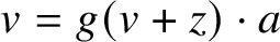 $v=g(v+z)\cdot a $
. Setting
$v=g(v+z)\cdot a $
. Setting
 $y=v+z$
we see that
$y=v+z$
we see that
 $v=g(y)\cdot a$
, say,
$v=g(y)\cdot a$
, say,
 $\widetilde \psi (y)= (z,a)$
and
$\widetilde \psi (y)= (z,a)$
and
 $\widetilde \psi $
is bijective. As we have
$\widetilde \psi $
is bijective. As we have
 $$ \begin{align*} a={v\over g(y)}={v\over g(v+z)} = {v\over g(z)}\cdot {g(z)\over g(v+z)}, \end{align*} $$
the map associating a to a pair
 $(z,v)$
is again rationally textile. This gives (b) and finishes the proof.
$(z,v)$
is again rationally textile. This gives (b) and finishes the proof.
(2) Division of deformations: To have an isomorphism
 $\psi _d$
as in assertion (b) of the preceding theorem it was necessary to restrict the set of vectors y to the stratum
$\psi _d$
as in assertion (b) of the preceding theorem it was necessary to restrict the set of vectors y to the stratum
 ${\mathcal S}_d$
. Otherwise, for arbitrary y, the order of
${\mathcal S}_d$
. Otherwise, for arbitrary y, the order of
 $g(y)$
may jump, so that the space of remainders could not be defined uniformly. Instead of working with a stratification and the Cartesian product decomposition
$g(y)$
may jump, so that the space of remainders could not be defined uniformly. Instead of working with a stratification and the Cartesian product decomposition
 ${\mathcal S}_d\cong {\mathcal Z}_d\times {\mathcal V}_d$
of the stratum
${\mathcal S}_d\cong {\mathcal Z}_d\times {\mathcal V}_d$
of the stratum
 ${\mathcal S}_d$
, one may also perform the division for series whose coefficients lie in a complete local ring; that is, for deformations of given power series vectors in
${\mathcal S}_d$
, one may also perform the division for series whose coefficients lie in a complete local ring; that is, for deformations of given power series vectors in
 $\mathcal A_{\circ }^m$
. In this case, no stratification is necessary. This kind of division will be explained in the second part of this section. First we need a couple of definitions.
$\mathcal A_{\circ }^m$
. In this case, no stratification is necessary. This kind of division will be explained in the second part of this section. First we need a couple of definitions.
Throughout the remainder of this section, only formal power series will be considered, so that
 $\mathcal A_{\circ }=\mathbf {k}_{\circ }[[\mathrm {t}]]$
,
$\mathcal A_{\circ }=\mathbf {k}_{\circ }[[\mathrm {t}]]$
,
 ${\mathcal B}=\mathbf {k}[[\mathrm {t},\mathrm {y}]]$
. The convergent case can be treated similarly but requires considerably more efforts; cf. Theorem 2, A.II.4, in [Reference HauserHa1].
${\mathcal B}=\mathbf {k}[[\mathrm {t},\mathrm {y}]]$
. The convergent case can be treated similarly but requires considerably more efforts; cf. Theorem 2, A.II.4, in [Reference HauserHa1].
Let S be a local ring, not necessarily Noetherian, with maximal ideal
 $M_S$
and residue field
$M_S$
and residue field
 $S/M_S=\mathbf {k}$
. It will always be equipped with a filtred topology defined by a decreasing sequence of ideals
$S/M_S=\mathbf {k}$
. It will always be equipped with a filtred topology defined by a decreasing sequence of ideals
 $J_k$
satisfying
$J_k$
satisfying
 $J_k\cdot J_{\ell }\subset J_{k+\ell }$
. We assume that
$J_k\cdot J_{\ell }\subset J_{k+\ell }$
. We assume that
 $M_S^k\subset J_k$
for all k and that S is complete. Further, to avoid complications, we assume that
$M_S^k\subset J_k$
for all k and that S is complete. Further, to avoid complications, we assume that
 $\mathbf {k}$
embeds into S as a field of coefficients.Footnote
22
Let us denote by
$\mathbf {k}$
embeds into S as a field of coefficients.Footnote
22
Let us denote by
 ${\mathcal A}_{S,\circ }=S_{\circ }[[\mathrm {t}]]$
the ring of formal power series in
${\mathcal A}_{S,\circ }=S_{\circ }[[\mathrm {t}]]$
the ring of formal power series in
 $\mathrm {t}$
with coefficients in S and without constant term (in S). Series in
$\mathrm {t}$
with coefficients in S and without constant term (in S). Series in
 ${\mathcal A}_{S,\circ }$
will be distinguished from series in
${\mathcal A}_{S,\circ }$
will be distinguished from series in
 $\mathcal A_{\circ }$
by a tilde. Taking the coefficients of a power series vector
$\mathcal A_{\circ }$
by a tilde. Taking the coefficients of a power series vector
 $\widetilde y\in {\mathcal A}_{S,\circ }^m$
modulo
$\widetilde y\in {\mathcal A}_{S,\circ }^m$
modulo
 $M_S$
gives a power series vector y in
$M_S$
gives a power series vector y in
 $\mathcal A_{\circ }^m$
, the reduction of
$\mathcal A_{\circ }^m$
, the reduction of
 $\widetilde y$
modulo
$\widetilde y$
modulo
 $M_S$
. A deformation of a vector
$M_S$
. A deformation of a vector
 $y\in \mathcal A_{\circ }^m$
over S is, by definition, a vector
$y\in \mathcal A_{\circ }^m$
over S is, by definition, a vector
 $\widetilde y\in {\mathcal A}_{S,\circ }^m$
whose reduction modulo
$\widetilde y\in {\mathcal A}_{S,\circ }^m$
whose reduction modulo
 $M_S$
equals y. The set of all deformations of y parametrised by S is denoted by
$M_S$
equals y. The set of all deformations of y parametrised by S is denoted by
 $({\mathcal A}_{S,\circ }^m,y)$
.Footnote
23
$({\mathcal A}_{S,\circ }^m,y)$
.Footnote
23
Theorem 3.6. Weierstrass division for deformations
We restrict to the case of formal power series. For a given power series
 $g\in {\mathcal B}$
, denote by
$g\in {\mathcal B}$
, denote by
 $w=g(y)\cdot a+z$
the Weierstrass division of a series
$w=g(y)\cdot a+z$
the Weierstrass division of a series
 $w\in \mathcal A_{\circ }$
by
$w\in \mathcal A_{\circ }$
by
 $g(y)$
for some
$g(y)$
for some
 $y\in \mathcal A_{\circ }^m$
for which
$y\in \mathcal A_{\circ }^m$
for which
 $g(y)$
is nonzero of order d, with
$g(y)$
is nonzero of order d, with
 $a\in \mathcal A_{\circ }$
and
$a\in \mathcal A_{\circ }$
and
 $z\in \mathbf {k}_{\circ }[\mathrm {t}]_{\leq d}$
. Let S be a complete local ring as before with maximal ideal
$z\in \mathbf {k}_{\circ }[\mathrm {t}]_{\leq d}$
. Let S be a complete local ring as before with maximal ideal
 $M_S$
and residue field
$M_S$
and residue field
 $S/M_S=\mathbf {k}$
embedding into S.
$S/M_S=\mathbf {k}$
embedding into S.
(a) For every vector
 $\widetilde y \in {\mathcal A}_{S,\circ }^m$
and every series
$\widetilde y \in {\mathcal A}_{S,\circ }^m$
and every series
 $\widetilde w\in {\mathcal A}_{S,\circ }$
, deformations of y and w respectively, there exist a unique power series
$\widetilde w\in {\mathcal A}_{S,\circ }$
, deformations of y and w respectively, there exist a unique power series
 $\widetilde a \in {\mathcal A}_{S,\circ }$
and a unique polynomial
$\widetilde a \in {\mathcal A}_{S,\circ }$
and a unique polynomial
 $\widetilde z \in S[\mathrm {t}]_{\leq d}$
of degree
$\widetilde z \in S[\mathrm {t}]_{\leq d}$
of degree
 $\leq d$
without constant term, both deformations of a and z respectively, such that
$\leq d$
without constant term, both deformations of a and z respectively, such that
 $$ \begin{align*} \widetilde w = g(\widetilde y) \cdot \widetilde a +\widetilde z. \end{align*} $$
(b) The coefficients of
 $\widetilde a$
and
$\widetilde a$
and
 $\widetilde z$
are the evaluations in the coefficients of
$\widetilde z$
are the evaluations in the coefficients of
 $\,\widetilde y$
and
$\,\widetilde y$
and
 $\widetilde w$
of formal power series.
$\widetilde w$
of formal power series.
The statement also holds for convergent series but is then more delicate to prove; see Theorem 2, A.II.4, in [Reference HauserHa1].
Proof. We show that the map
 $$ \begin{align*} \alpha:({\mathcal A}_{S,\circ}^m,a)\times (S[\mathrm{t}]_{\leq d},z) \rightarrow ({\mathcal A}_{S,\circ},w) \end{align*} $$
 $$ \begin{align*} (\widetilde a, \widetilde z)\rightarrow \widetilde w = g(\widetilde y) \cdot \widetilde a +\widetilde z \end{align*} $$
is an isomorphism. Using that
 $\mathbf {k}\subset S$
, we write
$\mathbf {k}\subset S$
, we write
 $\widetilde y= y+y^{\circ }$
with
$\widetilde y= y+y^{\circ }$
with
 $y^{\circ }\in M_S\cdot {\mathcal A}_{S,\circ }^m$
and, accordingly,
$y^{\circ }\in M_S\cdot {\mathcal A}_{S,\circ }^m$
and, accordingly,
 $g(\widetilde y)= g(y)+h(y,y^{\circ })$
with
$g(\widetilde y)= g(y)+h(y,y^{\circ })$
with
 $h\in \mathbf {k}_{\circ }[[\mathrm {t},\mathrm {y},\mathrm {y}^{\circ }]]$
, where
$h\in \mathbf {k}_{\circ }[[\mathrm {t},\mathrm {y},\mathrm {y}^{\circ }]]$
, where
 $\mathrm {y}^{\circ }=(\mathrm {y}_1^{\circ },\ldots ,\mathrm {y}_m^{\circ })$
denotes a new vector of variables. Observe here that
$\mathrm {y}^{\circ }=(\mathrm {y}_1^{\circ },\ldots ,\mathrm {y}_m^{\circ })$
denotes a new vector of variables. Observe here that
 $h(y,y^{\circ })\in M_S\cdot {\mathcal A}_{S,\circ }$
. By the assumption on y we can write
$h(y,y^{\circ })\in M_S\cdot {\mathcal A}_{S,\circ }$
. By the assumption on y we can write
 $g(y)=\mathrm {t}^d\cdot u$
with a unit
$g(y)=\mathrm {t}^d\cdot u$
with a unit
 $u\in \mathbf {k}[[\mathrm {t}]]$
. Without loss of generality, we may assume that
$u\in \mathbf {k}[[\mathrm {t}]]$
. Without loss of generality, we may assume that
 $u=1$
, say
$u=1$
, say
 $g(y)=\mathrm {t}^d$
. The map
$g(y)=\mathrm {t}^d$
. The map
 $$ \begin{align*} \gamma(\widetilde a, \widetilde z)\rightarrow [ g(y)-g(\widetilde y)] \cdot \widetilde a \end{align*} $$
is the multiplication of
 $\widetilde a$
with
$\widetilde a$
with
 $\mathrm {t}^d-g(\widetilde y)= g(y)-g(\widetilde y)=h(y,y^{\circ })\in M_S\cdot {\mathcal A}_{S,\circ }$
. The map
$\mathrm {t}^d-g(\widetilde y)= g(y)-g(\widetilde y)=h(y,y^{\circ })\in M_S\cdot {\mathcal A}_{S,\circ }$
. The map
 $\beta $
given by
$\beta $
given by
 $\beta (\widetilde a, \widetilde z)= \mathrm {t}^d\cdot \widetilde a + \widetilde z$
is clearly an isomorphism. It therefore suffices to show that
$\beta (\widetilde a, \widetilde z)= \mathrm {t}^d\cdot \widetilde a + \widetilde z$
is clearly an isomorphism. It therefore suffices to show that
 $$ \begin{align*} \alpha\circ\beta^{-1} =\mathrm{Id}_{({\mathcal A}_{S,\circ},w)} - \gamma\circ\beta^{-1} \end{align*} $$
is an isomorphism. To see this, observe first that the map
 $\gamma \circ \beta ^{-1}$
sends the maximal ideal
$\gamma \circ \beta ^{-1}$
sends the maximal ideal
 $M_S\cdot {\mathcal A}_{S,\circ }$
of
$M_S\cdot {\mathcal A}_{S,\circ }$
of
 ${\mathcal A}_{S,\circ }$
into
${\mathcal A}_{S,\circ }$
into
 $M_S^2\cdot {\mathcal A}_{S,\circ }$
. Therefore, the geometric series in
$M_S^2\cdot {\mathcal A}_{S,\circ }$
. Therefore, the geometric series in
 $\gamma \circ \beta ^{-1}$
, say
$\gamma \circ \beta ^{-1}$
, say
 $$ \begin{align*} \delta=\sum_{k=0}^{\infty} (\gamma\circ\beta^{-1})^k, \end{align*} $$
induces, by the completeness of S, a well-defined map
 $\delta :{\mathcal A}_{S,\circ }\rightarrow {\mathcal A}_{S,\circ }$
which is the inverse to
$\delta :{\mathcal A}_{S,\circ }\rightarrow {\mathcal A}_{S,\circ }$
which is the inverse to
 $\alpha \circ \beta ^{-1}$
. This proves the theorem.
$\alpha \circ \beta ^{-1}$
. This proves the theorem.
Remark 3.7. In the above division, the coefficients of the expansion of
 $\widetilde w$
and
$\widetilde w$
and
 $\widetilde y$
with respect to
$\widetilde y$
with respect to
 $\mathrm {t}$
are treated as variables, so the division is in this sense universal. One may then evaluate the variables by taking any elements of the maximal ideal of a complete local ring S in order to obtain a corresponding division for deformations of w and y over S.
$\mathrm {t}$
are treated as variables, so the division is in this sense universal. One may then evaluate the variables by taking any elements of the maximal ideal of a complete local ring S in order to obtain a corresponding division for deformations of w and y over S.
We will apply the preceding theorem to the division of the components
 $\widetilde y_j$
of a deformation
$\widetilde y_j$
of a deformation
 $\widetilde y$
of
$\widetilde y$
of
 $y\in \mathcal A_{\circ }^m$
by
$y\in \mathcal A_{\circ }^m$
by
 $g(\widetilde y)$
analogously as we did in the first part of this section with y itself. Let
$g(\widetilde y)$
analogously as we did in the first part of this section with y itself. Let
 $y\in \mathcal A_{\circ }^m$
be given with
$y\in \mathcal A_{\circ }^m$
be given with
 $g(y)\neq 0$
of order d and induced division
$g(y)\neq 0$
of order d and induced division
 $y=g(y)\cdot a+z$
with
$y=g(y)\cdot a+z$
with
 $a\in \mathcal A_{\circ }^m$
and
$a\in \mathcal A_{\circ }^m$
and
 $z\in {\mathcal Z}_d$
as in Theorem 3.4.
$z\in {\mathcal Z}_d$
as in Theorem 3.4.
Theorem 3.8. For a given power series
 $g(\mathrm {t},\mathrm {y})\in {\mathcal B}$
denote by
$g(\mathrm {t},\mathrm {y})\in {\mathcal B}$
denote by
 $y=g(y)\cdot a+z$
the componentwise Weierstrass division of a vector
$y=g(y)\cdot a+z$
the componentwise Weierstrass division of a vector
 $y\in \mathcal A_{\circ }^m$
by
$y\in \mathcal A_{\circ }^m$
by
 $g(y)$
for some y for which
$g(y)$
for some y for which
 $g(y)$
is nonzero of order d, with
$g(y)$
is nonzero of order d, with
 $a\in \mathcal A_{\circ }^m$
and
$a\in \mathcal A_{\circ }^m$
and
 $z\in (\mathbf {k}_{\circ }[\mathrm {t}]]_{\leq d})^m$
.
$z\in (\mathbf {k}_{\circ }[\mathrm {t}]]_{\leq d})^m$
.
(a) For every deformation
 $\widetilde y \in ({\mathcal A}_{S,\circ }^m,y)$
of y there exist a unique power series vector
$\widetilde y \in ({\mathcal A}_{S,\circ }^m,y)$
of y there exist a unique power series vector
 $\widetilde a \in {\mathcal A}_{S,\circ }^m$
and a unique polynomial vector
$\widetilde a \in {\mathcal A}_{S,\circ }^m$
and a unique polynomial vector
 $\widetilde z \in (S[\mathrm {t}]_{\leq d})^m$
without constant term, both deformations of a and z respectively, such that
$\widetilde z \in (S[\mathrm {t}]_{\leq d})^m$
without constant term, both deformations of a and z respectively, such that
 $$ \begin{align*} \widetilde y = g(\widetilde y) \cdot \widetilde a +\widetilde z. \end{align*} $$
(b) The coefficients of
 $\widetilde a$
and
$\widetilde a$
and
 $\widetilde z$
are formal power series in the coefficients of
$\widetilde z$
are formal power series in the coefficients of
 $\widetilde y$
.
$\widetilde y$
.
Proof. Both assertions follow from Theorem 3.6.
Remarks 3.9. (a) The statement is not a local version of the classical division theorem 3.4 since the deformations of y are not confined to the stratum
 ${\mathcal S}_d$
.
${\mathcal S}_d$
.
(b) The division does not hold for local rings S which are not complete. It suffices to divide
 $\mathrm {t}^d$
by the deformation
$\mathrm {t}^d$
by the deformation
 $\mathrm {t}^d+s_1\cdot \mathrm {t}^{d-1}+s_2\cdot \mathrm {t}^{d+1}$
of
$\mathrm {t}^d+s_1\cdot \mathrm {t}^{d-1}+s_2\cdot \mathrm {t}^{d+1}$
of
 $\mathrm {t}^d$
, with
$\mathrm {t}^d$
, with
 $s_1,s_2\in M_S$
, to see that the remainder has as coefficients genuine power series in elements of
$s_1,s_2\in M_S$
, to see that the remainder has as coefficients genuine power series in elements of
 $M_S$
.
$M_S$
.
4 Division modules
This section can be skipped on first reading. The proofs of the factorisation and linearisation theorems are based on the decomposition of a power series vector
 $y\in \mathcal A_{\circ }^m$
into a sum
$y\in \mathcal A_{\circ }^m$
into a sum
 $y=v+z$
where z belongs to a finite-dimensional space of polynomial vectors and where v is the part of y on which the linearisation can be achieved. The decomposition is done by the componentwise Weierstrass division of y by a suitable divisor. This section characterises possible choices of such divisors.
$y=v+z$
where z belongs to a finite-dimensional space of polynomial vectors and where v is the part of y on which the linearisation can be achieved. The decomposition is done by the componentwise Weierstrass division of y by a suitable divisor. This section characterises possible choices of such divisors.
Definition 4.1. A division module for a vector
 $f=f(\mathrm {t},\mathrm {y})\in {\mathcal B}^k$
is a
$f=f(\mathrm {t},\mathrm {y})\in {\mathcal B}^k$
is a
 $\mathcal B_{\circ }$
-submodule
$\mathcal B_{\circ }$
-submodule
 ${\mathcal G}$
of
${\mathcal G}$
of
 $\mathcal B_{\circ }^m$
, with
$\mathcal B_{\circ }^m$
, with
 $\mathcal B_{\circ }={\mathcal B}\cap \mathbf {k}_{\circ }[[\mathrm {t},\mathrm {y}]]$
, which is a Cartesian product
$\mathcal B_{\circ }={\mathcal B}\cap \mathbf {k}_{\circ }[[\mathrm {t},\mathrm {y}]]$
, which is a Cartesian product
 $$ \begin{align*} {\mathcal G}= \langle g_1\rangle \times \ldots\times \langle g_m\rangle \subset\mathcal B_{\circ}^m \end{align*} $$
of nonzero principal ideals
 $\langle g_i\rangle :=g_i\cdot \mathcal B_{\circ }$
of
$\langle g_i\rangle :=g_i\cdot \mathcal B_{\circ }$
of
 $\mathcal B_{\circ }$
, with
$\mathcal B_{\circ }$
, with
 $g_i\in {\mathcal B}$
, satisfying the following conditions:
$g_i\in {\mathcal B}$
, satisfying the following conditions:
-
(i) For all
 $z\in \mathcal A_{\circ }^m$
and
$v\in {\mathcal G}(z):= g_1(z)\cdot \mathcal A_{\circ } \times \ldots \times g_m(z)\cdot \mathcal A_{\circ }\subset \mathcal A_{\circ }^m$
we have
$$ \begin{align*} {\mathcal G}(z)={\mathcal G}(z+v). \end{align*} $$
$z\in \mathcal A_{\circ }^m$
and
$v\in {\mathcal G}(z):= g_1(z)\cdot \mathcal A_{\circ } \times \ldots \times g_m(z)\cdot \mathcal A_{\circ }\subset \mathcal A_{\circ }^m$
we have
$$ \begin{align*} {\mathcal G}(z)={\mathcal G}(z+v). \end{align*} $$
-
(ii) Write elements v of
${\mathcal G}(z)$
as
$v=\Delta _g(z)\cdot a$
with column vector
$a\in \mathcal A_{\circ }^m$
and a diagonal matrix
$\Delta _g=\mathrm {diag}(g_1,\ldots ,g_m)\in {\mathcal B}^{m\times m}$
. There exists a (formal, convergent, respectively algebraic) power series vector
$p\in \mathbf {k}[[\mathrm {t},\mathrm {z},\mathrm {a}]]^m$
in three sets of variables
$\mathrm {t}$
,
$\mathrm {z}=(\mathrm {z}_1,\ldots ,\mathrm {z}_m)$
and
$\mathrm {a}=(\mathrm {a}_1,\ldots ,\mathrm {a}_m)$
, which is at least of order
$2$
in
$\mathrm {a}$
and satisfies for all z,
$a\in \mathcal A_{\circ }^m$
,
$$ \begin{align*} f(z+\Delta_g(z)\cdot a) = f(z)+{\partial}_{\mathrm{y}}f(z)\cdot \Delta_g(z)\cdot a+{\partial}_{\mathrm{y}}f(z)\cdot \Delta_g(z)\cdot p(z,a). \end{align*} $$


Remarks 4.2. (a) Condition (i) can be rewritten as an equality of ideals in
 $\mathcal A_{\circ }$
, say
$\mathcal A_{\circ }$
, say
 $\langle g_i(z)\rangle =\langle g_i(z+\Delta _g(z)\cdot a)\rangle $
, for all z and a in
$\langle g_i(z)\rangle =\langle g_i(z+\Delta _g(z)\cdot a)\rangle $
, for all z and a in
 $\mathcal A_{\circ }^m$
, and
$\mathcal A_{\circ }^m$
, and
 $i=1,\ldots ,m$
. Phrased differently, there exists an invertible matrix
$i=1,\ldots ,m$
. Phrased differently, there exists an invertible matrix
 $U\in \mathrm {Gl}_m(\mathbf {k}[[\mathrm {t},\mathrm {z},\mathrm {a}]])$
(with formal, convergent, respectively algebraic entries) such that
$U\in \mathrm {Gl}_m(\mathbf {k}[[\mathrm {t},\mathrm {z},\mathrm {a}]])$
(with formal, convergent, respectively algebraic entries) such that
 $$ \begin{align*} \Delta_g(z) = \Delta_g(z+\Delta_g(z)\cdot a)\cdot U(z,a) \end{align*} $$
holds for all z and a.
(b) Condition (i) appears in Lemma 3.2, which is used in the proof of Theorem 3.4 and in the proof of Proposition 5.2.
(c) Condition (ii) ensures that the terms of order
 $\geq 2$
of the Taylor expansion of
$\geq 2$
of the Taylor expansion of
 $f(z+\Delta _g(z)\cdot a)$
belong to the module generated by the linear terms
$f(z+\Delta _g(z)\cdot a)$
belong to the module generated by the linear terms
 ${\partial }_{\mathrm {y}}f(z)\cdot \Delta _g(z)\cdot a$
. This module equals the
${\partial }_{\mathrm {y}}f(z)\cdot \Delta _g(z)\cdot a$
. This module equals the
 $\mathcal A_{\circ }$
-submodule
$\mathcal A_{\circ }$
-submodule
 ${\partial }_{\mathrm {y}}f(z)\cdot {\mathcal G}(z)$
of
${\partial }_{\mathrm {y}}f(z)\cdot {\mathcal G}(z)$
of
 $\mathcal A_{\circ }^k$
which is the image of
$\mathcal A_{\circ }^k$
which is the image of
 ${\mathcal G}(z)$
under the tangent map at z of the arquile map
${\mathcal G}(z)$
under the tangent map at z of the arquile map
 ${f_{\infty }}:\mathcal A_{\circ }^m\rightarrow \mathcal A_{\circ }^k$
induced by f. In the terminology of [Reference Bruschek and HauserBH], condition (ii) signifies that for each
${f_{\infty }}:\mathcal A_{\circ }^m\rightarrow \mathcal A_{\circ }^k$
induced by f. In the terminology of [Reference Bruschek and HauserBH], condition (ii) signifies that for each
 $z \in \mathcal A_{\circ }^m$
, the map
$z \in \mathcal A_{\circ }^m$
, the map
 $$ \begin{align*} \alpha_z:{\mathcal G}(z)\rightarrow \mathcal A_{\circ}^k,\,v=\Delta_g(z)\cdot a\rightarrow f(z+\Delta_g(z)\cdot a) \end{align*} $$
is a quasi-submersion; that is, that its image is contained in the image of the tangent map. More generally speaking, it is a map of constant rank in the sense of [Reference Hauser and MüllerHM]. This is a necessary condition to be ‘locally linearisable’. To make this precise and to prove that with the appropriate assumptions this is also a sufficient condition – that is, that the map
 $\alpha _z$
is indeed linearisable (in a specific sense) – will be the subject of Section 5.
$\alpha _z$
is indeed linearisable (in a specific sense) – will be the subject of Section 5.
(d) Note that
 $\Delta _g(z)\cdot a$
is just the vector
$\Delta _g(z)\cdot a$
is just the vector
 $(g_1(z)\cdot a_1,\ldots ,g_m(z)\cdot a_m)\in \mathcal A_{\circ }^m$
and that the series
$(g_1(z)\cdot a_1,\ldots ,g_m(z)\cdot a_m)\in \mathcal A_{\circ }^m$
and that the series
 $g_i$
may have nonzero constant term
$g_i$
may have nonzero constant term
 $g_i(0)$
.
$g_i(0)$
.
(e) The name ‘division module’ is motivated by the later decomposition of vectors
 $y\in \mathcal A_{\circ }^m$
into
$y\in \mathcal A_{\circ }^m$
into
 $y=\Delta _g(y)\cdot \widetilde a+z=\Delta _g(z)\cdot a+z$
given by the Weierstrass division of the components
$y=\Delta _g(y)\cdot \widetilde a+z=\Delta _g(z)\cdot a+z$
given by the Weierstrass division of the components
 $y_i$
by
$y_i$
by
 $g_i(y)$
; see Proposition 5.2.
$g_i(y)$
; see Proposition 5.2.
Example. Typically, one could take for
 ${\mathcal G}$
the m-fold Cartesian product
${\mathcal G}$
the m-fold Cartesian product
 $$ \begin{align*} {\mathcal G}=\langle g^{o_1}\rangle\times \ldots\times \langle g^{o_m}\rangle \end{align*} $$
of ideals of
 $\mathcal B_{\circ }$
for some chosen nonzero series
$\mathcal B_{\circ }$
for some chosen nonzero series
 $g\in {\mathcal B}$
and nonnegative integers
$g\in {\mathcal B}$
and nonnegative integers
 $o_i$
. It is easy to see that such a
$o_i$
. It is easy to see that such a
 ${\mathcal G}$
satisfies condition (i) of the definition. However, condition (ii) will not hold without extra assumptions on g. These are specified in the next result.
${\mathcal G}$
satisfies condition (i) of the definition. However, condition (ii) will not hold without extra assumptions on g. These are specified in the next result.
Proposition 4.3. Let
 $f\in {\mathcal B}^k$
be given. Assume that
$f\in {\mathcal B}^k$
be given. Assume that
 $k\leq m$
and that some
$k\leq m$
and that some
 $(k\times k)$
-minor g of the relative Jacobian matrix
$(k\times k)$
-minor g of the relative Jacobian matrix
 ${\partial }_{\mathrm {y}} f$
of f is not zero. For any choice of nonnegative integers
${\partial }_{\mathrm {y}} f$
of f is not zero. For any choice of nonnegative integers
 $o_1,\ldots ,o_m$
satisfying
$o_1,\ldots ,o_m$
satisfying
 $$ \begin{align*} o_i+o_j\geq o_l+1 \end{align*} $$
for all
 $i,j\in \{1,\cdots ,m\}$
and
$i,j\in \{1,\cdots ,m\}$
and
 $\ell \in \{1,\ldots ,k\}$
, the
$\ell \in \{1,\ldots ,k\}$
, the
 $\mathcal B_{\circ }$
-module
$\mathcal B_{\circ }$
-module
 $$ \begin{align*} {\mathcal G}=\langle g^{o_1}\rangle\times\ldots\times\langle g^{o_m}\rangle\subset\mathcal B_{\circ}^m \end{align*} $$
is a division module for f.
Remark 4.4. This proposition will be used later on in the case where
 $o_i=1$
for
$o_i=1$
for
 $1\leq i\leq k$
and
$1\leq i\leq k$
and
 $o_i=2$
for
$o_i=2$
for
 $k+1\leq i\leq m$
.
$k+1\leq i\leq m$
.
Proof. For condition (i), it suffices to show, since
 ${\mathcal G}$
is a Cartesian product of principal ideals, that for any
${\mathcal G}$
is a Cartesian product of principal ideals, that for any
 $z\in \mathcal A_{\circ }^m$
and
$z\in \mathcal A_{\circ }^m$
and
 $v\in {\mathcal G}(z)$
we have the equality of ideals
$v\in {\mathcal G}(z)$
we have the equality of ideals
 $$ \begin{align*} \langle g(z)\rangle=\langle g(z+v)\rangle \end{align*} $$
in
 $\mathcal A_{\circ }$
. This equality does not use that g is a minor – it is the content of Lemma 3.2.
$\mathcal A_{\circ }$
. This equality does not use that g is a minor – it is the content of Lemma 3.2.
To prove that
 ${\mathcal G}$
fulfils condition (ii), let
${\mathcal G}$
fulfils condition (ii), let
 $v=\Delta _g(z)\cdot a\in {\mathcal G}(z)$
with
$v=\Delta _g(z)\cdot a\in {\mathcal G}(z)$
with
 $a\in \mathcal A_{\circ }^m$
. Taylor expansion gives
$a\in \mathcal A_{\circ }^m$
. Taylor expansion gives
 $$ \begin{align*} f(z+\Delta_g(z)\cdot a)=f(z)+{\partial}_{\mathrm{y}} f(z)\cdot \Delta_g(z)\cdot a + q(z,\Delta_g(z)\cdot a) \end{align*} $$
with some vector
 $q\in \mathbf {k}[[\mathrm {t},\mathrm {z},\mathrm {w}]]^k$
which is of order at least 2 in
$q\in \mathbf {k}[[\mathrm {t},\mathrm {z},\mathrm {w}]]^k$
which is of order at least 2 in
 $\mathrm {w}=(\mathrm {w}_1,\ldots ,\mathrm {w}_m)$
. We have to find a power series vector
$\mathrm {w}=(\mathrm {w}_1,\ldots ,\mathrm {w}_m)$
. We have to find a power series vector
 $p\in \mathbf {k}[[\mathrm {t},\mathrm {z},\mathrm {a}]]^k$
of order at least two in
$p\in \mathbf {k}[[\mathrm {t},\mathrm {z},\mathrm {a}]]^k$
of order at least two in
 $\mathrm {a}=(\mathrm {a}_1,\ldots ,\mathrm {a}_m)$
such that
$\mathrm {a}=(\mathrm {a}_1,\ldots ,\mathrm {a}_m)$
such that
 $$ \begin{align*} q(z,\Delta_g(z)\cdot a) = {\partial}_y f(z)\cdot \Delta_g(z)\cdot p(z,a) \end{align*} $$
holds for all z and a in
 $\mathcal A_{\circ }^m$
. First observe that each component of
$\mathcal A_{\circ }^m$
. First observe that each component of
 $q(z,\Delta _g(z)\cdot a)$
belongs to the ideal of
$q(z,\Delta _g(z)\cdot a)$
belongs to the ideal of
 $\mathcal A_{\circ }$
generated by the powers
$\mathcal A_{\circ }$
generated by the powers
 $g(z)^{o_i+o_j}$
for
$g(z)^{o_i+o_j}$
for
 $i,j\in \{1,\ldots ,m\}$
. It therefore suffices to show that any vector of the form
$i,j\in \{1,\ldots ,m\}$
. It therefore suffices to show that any vector of the form
 $(0,\ldots ,0,g^{o_i+o_j},0,\ldots ,0)$
, with
$(0,\ldots ,0,g^{o_i+o_j},0,\ldots ,0)$
, with
 $i,j\in \{1,\cdots ,m\}$
, can be written as a
$i,j\in \{1,\cdots ,m\}$
, can be written as a
 $\mathcal B_{\circ }$
-linear combination of the vectors
$\mathcal B_{\circ }$
-linear combination of the vectors
 ${\partial }_{\mathrm {y}_1}f\cdot g^{o_1},\ldots ,{\partial }_{\mathrm {y}_k}f\cdot g^{o_k}$
.
${\partial }_{\mathrm {y}_1}f\cdot g^{o_1},\ldots ,{\partial }_{\mathrm {y}_k}f\cdot g^{o_k}$
.
To prove this, set
 $\mathrm {y}^1=(\mathrm {y}_1,\ldots ,\mathrm {y}_k)$
, so that g is without loss of generality the determinant of the
$\mathrm {y}^1=(\mathrm {y}_1,\ldots ,\mathrm {y}_k)$
, so that g is without loss of generality the determinant of the
 $(k\times k)$
-submatrix
$(k\times k)$
-submatrix
 ${\partial }_{\mathrm {y}^1}f$
of
${\partial }_{\mathrm {y}^1}f$
of
 ${\partial }_{\mathrm {y}} f$
. Denote by
${\partial }_{\mathrm {y}} f$
. Denote by
 ${\partial }^*_{\mathrm {y}^1}f$
the adjoint matrix of
${\partial }^*_{\mathrm {y}^1}f$
the adjoint matrix of
 ${\partial }_{\mathrm {y}^1}f$
. We then have
${\partial }_{\mathrm {y}^1}f$
. We then have
 ${\partial }_{\mathrm {y}^1}f\cdot {\partial }^*_{\mathrm {y}^1}f=g\cdot {1\!\! 1}_k$
and, accordingly,
${\partial }_{\mathrm {y}^1}f\cdot {\partial }^*_{\mathrm {y}^1}f=g\cdot {1\!\! 1}_k$
and, accordingly,
 $g^o\cdot {\partial }_{\mathrm {y}^1}f\cdot {\partial }^*_{\mathrm {y}^1}f=g^{o+1}\cdot {1\!\! 1}_k$
for any integer o. Taking now for o the values
$g^o\cdot {\partial }_{\mathrm {y}^1}f\cdot {\partial }^*_{\mathrm {y}^1}f=g^{o+1}\cdot {1\!\! 1}_k$
for any integer o. Taking now for o the values
 $o_i+o_j-1$
and using the assumption that
$o_i+o_j-1$
and using the assumption that
 $o_i+o_j\geq o_l+1$
for all
$o_i+o_j\geq o_l+1$
for all
 $i,j\in \{1,\cdots ,m\}$
and
$i,j\in \{1,\cdots ,m\}$
and
 $\ell \in \{1,\ldots ,k\}$
, we get the claim. This establishes condition (ii).
$\ell \in \{1,\ldots ,k\}$
, we get the claim. This establishes condition (ii).
5 Linearisation theorem
This is the central section of the article. To prepare the setting of the linearisation theorem below, let
 $f=(f_1,\ldots ,f_k)\in {\mathcal B}^k$
be a vector of power series which admits a division module
$f=(f_1,\ldots ,f_k)\in {\mathcal B}^k$
be a vector of power series which admits a division module
 ${\mathcal G}=\langle g_1\rangle \times \ldots \times \langle g_m\rangle \subset \mathcal B_{\circ }^m$
. Recall that by Proposition 4.3 the existence of such a module is ensured, for instance, in the case where
${\mathcal G}=\langle g_1\rangle \times \ldots \times \langle g_m\rangle \subset \mathcal B_{\circ }^m$
. Recall that by Proposition 4.3 the existence of such a module is ensured, for instance, in the case where
 $k\leq m$
and if there exists a nonzero
$k\leq m$
and if there exists a nonzero
 $(k\times k)$
-minor g of
$(k\times k)$
-minor g of
 ${\partial }_{\mathrm {y}} f$
. Up to a permutation of the variables we may assume that g is given by the first k columns of
${\partial }_{\mathrm {y}} f$
. Up to a permutation of the variables we may assume that g is given by the first k columns of
 ${\partial }_{\mathrm {y}} f$
. By Proposition 4.3, the
${\partial }_{\mathrm {y}} f$
. By Proposition 4.3, the
 $\mathcal B_{\circ }$
-module
$\mathcal B_{\circ }$
-module
 ${\mathcal G}=\langle g^{o_1}\rangle \times \ldots \times \langle g^{o_m}\rangle $
with
${\mathcal G}=\langle g^{o_1}\rangle \times \ldots \times \langle g^{o_m}\rangle $
with
 $o_i+o_j\geq o_l+1$
for all
$o_i+o_j\geq o_l+1$
for all
 $i,j\in \{1,\cdots ,m\}$
and
$i,j\in \{1,\cdots ,m\}$
and
 $\ell \in \{1,\ldots ,k\}$
is a division module for f.
$\ell \in \{1,\ldots ,k\}$
is a division module for f.
The following constructions (until the next lemma) hold for any vector
 $g\in {\mathcal B}^m$
. For a chosen m-tuple
$g\in {\mathcal B}^m$
. For a chosen m-tuple
 $\mathbf { d}=(d_1,\ldots ,d_m)\in {\mathbb N}^m$
, set
$\mathbf { d}=(d_1,\ldots ,d_m)\in {\mathbb N}^m$
, set
 $$ \begin{align*} {\mathcal S}_{\mathbf{d}}=\{y\in \mathcal A_{\circ}^m,\, g_i(y)\neq 0,\, \mathrm{ord}\,g_i(y)=d_i \text { for all } i\}. \end{align*} $$
Since
 $\mathrm {t}$
is just a single variable, the condition
$\mathrm {t}$
is just a single variable, the condition
 $\mathrm {ord}\,g_i(y)=d_i$
is equivalent to saying that
$\mathrm {ord}\,g_i(y)=d_i$
is equivalent to saying that
 $g_i(y)$
equals the monomial
$g_i(y)$
equals the monomial
 $\mathrm {t}^{d_i}$
up to the multiplication by a unit in
$\mathrm {t}^{d_i}$
up to the multiplication by a unit in
 $\mathcal A$
; that is, that
$\mathcal A$
; that is, that
 $\langle g_i(y)\rangle =\langle \mathrm {t}^{d_i}\rangle $
as ideals of
$\langle g_i(y)\rangle =\langle \mathrm {t}^{d_i}\rangle $
as ideals of
 $\mathcal A_{\circ }$
, for each
$\mathcal A_{\circ }$
, for each
 $y\in {\mathcal S}_{\mathbf {d}}$
. This implies that
$y\in {\mathcal S}_{\mathbf {d}}$
. This implies that
 ${\mathcal S}_{\mathbf {d}}$
is a cofinite textile locally closed subset of
${\mathcal S}_{\mathbf {d}}$
is a cofinite textile locally closed subset of
 $\mathcal A_{\circ }^m$
. It is
$\mathcal A_{\circ }^m$
. It is
 $\mathrm {t}$
-adically open since
$\mathrm {t}$
-adically open since
 ${\mathcal S}_{\mathbf {d}}$
contains with every element y the
${\mathcal S}_{\mathbf {d}}$
contains with every element y the
 $\mathrm {t}$
-adic neighbourhood
$\mathrm {t}$
-adic neighbourhood
 $y+\langle \mathrm {t}^{d_1}\rangle \times \ldots \times \langle \mathrm {t}^{d_m}\rangle $
in
$y+\langle \mathrm {t}^{d_1}\rangle \times \ldots \times \langle \mathrm {t}^{d_m}\rangle $
in
 $\mathcal A_{\circ }^m$
. We agree to set
$\mathcal A_{\circ }^m$
. We agree to set
 $\mathrm {ord}\,g_i(y)=\infty $
if
$\mathrm {ord}\,g_i(y)=\infty $
if
 $g_i(y)=0$
and then define accordingly
$g_i(y)=0$
and then define accordingly
 ${\mathcal S}_{\mathbf {d}}$
also if some
${\mathcal S}_{\mathbf {d}}$
also if some
 $d_i=\infty $
. This gives a countable partition of
$d_i=\infty $
. This gives a countable partition of
 $\mathcal A_{\circ }^m$
into
$\mathcal A_{\circ }^m$
into
 $$ \begin{align*} \mathcal A_{\circ}^m=\bigcup_{\mathbf{d}\in({\mathbb N}\cup\{\infty\})^m} {\mathcal S}_{\mathbf{d}}. \end{align*} $$
Restrict now to m-tuples
 $\mathbf {d}\in {\mathbb N}^m$
and vectors
$\mathbf {d}\in {\mathbb N}^m$
and vectors
 $y\in {\mathcal S}_{\mathbf {d}}$
. We set
$y\in {\mathcal S}_{\mathbf {d}}$
. We set
 $$ \begin{align*} {\mathcal V}_{\mathbf{d}}={\mathcal G}(y)=\langle\mathrm{t}^{d_1}\rangle\times \ldots\times \langle\mathrm{t}^{d_m}\rangle\subset\mathcal A_{\circ}^m. \end{align*} $$
We consider
 ${\mathcal V}_{\mathbf {d}}$
as an
${\mathcal V}_{\mathbf {d}}$
as an
 $\mathcal A_{\circ }$
-submodule of
$\mathcal A_{\circ }$
-submodule of
 $\mathcal A_{\circ }^m$
. Let
$\mathcal A_{\circ }^m$
. Let
 ${\mathcal R}_{\mathbf {d}}$
be the direct monomial complement of
${\mathcal R}_{\mathbf {d}}$
be the direct monomial complement of
 ${\mathcal V}_{\mathbf {d}}$
in
${\mathcal V}_{\mathbf {d}}$
in
 $\mathcal A_{\circ }^m$
consisting of vectors
$\mathcal A_{\circ }^m$
consisting of vectors
 $z\in \mathcal A_{\circ }^m$
whose ith component
$z\in \mathcal A_{\circ }^m$
whose ith component
 $z_i$
is a polynomial in
$z_i$
is a polynomial in
 $\mathbf {k}_{\circ }[\mathrm {t}]$
of degree
$\mathbf {k}_{\circ }[\mathrm {t}]$
of degree
 $\leq d_i$
,
$\leq d_i$
,
 $$ \begin{align*} {\mathcal R}_{\mathbf{d}}=\mathbf{k}_{\circ}[\mathrm{t}]_{\leq d_1}\times \ldots\times \mathbf{k}_{\circ}[\mathrm{t}]_{\leq d_m}, \end{align*} $$
with direct sum decomposition
 $$ \begin{align*} {\mathcal V}_{\mathbf{d}}\oplus{\mathcal R}_{\mathbf{d}}=\mathcal A_{\circ}^m. \end{align*} $$
Accordingly, we decompose vectors
 $y\in {\mathcal S}_{\mathbf {d}}$
into
$y\in {\mathcal S}_{\mathbf {d}}$
into
 $y=v+z$
with
$y=v+z$
with
 $v\in {\mathcal V}_{\mathbf {d}}$
and
$v\in {\mathcal V}_{\mathbf {d}}$
and
 $z\in {\mathcal R}_{\mathbf {d}}$
. The ith component
$z\in {\mathcal R}_{\mathbf {d}}$
. The ith component
 $z_i$
of z is the remainder of the Weierstrass division of the ith component
$z_i$
of z is the remainder of the Weierstrass division of the ith component
 $y_i$
of y with respect to
$y_i$
of y with respect to
 $\mathrm {t}^{d_i}$
; cf. Theorem 3.4. Denote by
$\mathrm {t}^{d_i}$
; cf. Theorem 3.4. Denote by
 $$ \begin{align*} \pi_{\mathbf{d}}:{\mathcal S}_{\mathbf{d}}\rightarrow {\mathcal R}_{\mathbf{d}},\,y\rightarrow z, \end{align*} $$
the induced textile map. Set
 $$ \begin{align*} {\mathcal Z}_{\mathbf{d}}={\mathcal S}_{\mathbf{d}}\cap {\mathcal R}_{\mathbf{d}}=\{z\in {\mathcal R}_{\mathbf{d}},\, g_i(z)\neq 0 \text{ and }\mathrm{ord}\,g_i(z)=d_i \text { for all } i\}. \end{align*} $$
Note that
 ${\mathcal R}_{\mathbf {d}}$
is a finite-dimensional
${\mathcal R}_{\mathbf {d}}$
is a finite-dimensional
 $\mathbf {k}$
-vector space of dimension
$\mathbf {k}$
-vector space of dimension
 $d_1+\ldots +d_m$
which will be considered as affine space
$d_1+\ldots +d_m$
which will be considered as affine space
 ${\mathcal R}_{\mathbf {d}}\cong \mathbb A_{\mathbf {k}}^{d_1+\ldots +d_m}$
, and
${\mathcal R}_{\mathbf {d}}\cong \mathbb A_{\mathbf {k}}^{d_1+\ldots +d_m}$
, and
 ${\mathcal Z}_d$
is a Zariski locally closed subset. Both
${\mathcal Z}_d$
is a Zariski locally closed subset. Both
 ${\mathcal V}_{\mathbf {d}}$
and
${\mathcal V}_{\mathbf {d}}$
and
 ${\mathcal R}_{\mathbf {d}}$
only depend on
${\mathcal R}_{\mathbf {d}}$
only depend on
 $\mathbf {d}=(d_1,\ldots ,d_m)$
. The sets
$\mathbf {d}=(d_1,\ldots ,d_m)$
. The sets
 ${\mathcal S}_{\mathbf {d}}$
and
${\mathcal S}_{\mathbf {d}}$
and
 ${\mathcal Z}_{\mathbf {d}}$
will depend on f in the situation of Proposition 4.3 where the series
${\mathcal Z}_{\mathbf {d}}$
will depend on f in the situation of Proposition 4.3 where the series
 $g_i=g^{o_i}$
are chosen as powers of a minor g of
$g_i=g^{o_i}$
are chosen as powers of a minor g of
 ${\partial }_{\mathrm {y}} f$
.
${\partial }_{\mathrm {y}} f$
.
Lemma 5.1. Let
 $f\in {\mathcal B}^k$
be a power series vector with division module
$f\in {\mathcal B}^k$
be a power series vector with division module
 ${\mathcal G}\subset \mathcal B_{\circ }^m$
, and let
${\mathcal G}\subset \mathcal B_{\circ }^m$
, and let
 $\mathbf {d}\in {\mathbb N}^m$
. The associated projection map
$\mathbf {d}\in {\mathbb N}^m$
. The associated projection map
 $\pi _{\mathbf {d}}:{\mathcal S}_{\mathbf {d}}\rightarrow {\mathcal R}_{\mathbf {d}},\,y\rightarrow z$
, has image
$\pi _{\mathbf {d}}:{\mathcal S}_{\mathbf {d}}\rightarrow {\mathcal R}_{\mathbf {d}},\,y\rightarrow z$
, has image
 ${\mathcal Z}_{\mathbf {d}}$
.
${\mathcal Z}_{\mathbf {d}}$
.
Said differently, if
 $y\in \mathcal A_{\circ }^m$
satisfies
$y\in \mathcal A_{\circ }^m$
satisfies
 $\mathrm {ord}\, g_i(y)=d_i$
for all i, then its remainder z satisfies the same condition.
$\mathrm {ord}\, g_i(y)=d_i$
for all i, then its remainder z satisfies the same condition.
Proof. Write
 $y=v+z$
as above. By Definition 4.1 (i) of division modules we know that
$y=v+z$
as above. By Definition 4.1 (i) of division modules we know that
 ${\mathcal G}(z)={\mathcal G}(y-v)={\mathcal G}(y)$
so that
${\mathcal G}(z)={\mathcal G}(y-v)={\mathcal G}(y)$
so that
 $z\in {\mathcal S}_{\mathbf {d}}$
. This proves that the image of
$z\in {\mathcal S}_{\mathbf {d}}$
. This proves that the image of
 $\pi $
is included in
$\pi $
is included in
 ${\mathcal Z}_{\mathbf {d}}={\mathcal S}_{\mathbf {d}}\cap {\mathcal R}_{\mathbf {d}}$
. It is whole
${\mathcal Z}_{\mathbf {d}}={\mathcal S}_{\mathbf {d}}\cap {\mathcal R}_{\mathbf {d}}$
. It is whole
 ${\mathcal Z}_{\mathbf {d}}$
since the restriction of
${\mathcal Z}_{\mathbf {d}}$
since the restriction of
 $\pi _{\mathbf {d}}$
to
$\pi _{\mathbf {d}}$
to
 ${\mathcal Z}_{\mathbf {d}}$
is the identity map.
${\mathcal Z}_{\mathbf {d}}$
is the identity map.
Proposition 5.2. Let
 $f\in {\mathcal B}^k$
be a power series vector with division module
$f\in {\mathcal B}^k$
be a power series vector with division module
 ${\mathcal G}\subset \mathcal B_{\circ }^m$
; diagonal matrix
${\mathcal G}\subset \mathcal B_{\circ }^m$
; diagonal matrix
 $\Delta _g$
; associated sets
$\Delta _g$
; associated sets
 ${\mathcal S}_{\mathbf {d}}$
,
${\mathcal S}_{\mathbf {d}}$
,
 ${\mathcal V}_{\mathbf {d}}$
,
${\mathcal V}_{\mathbf {d}}$
,
 ${\mathcal R}_{\mathbf {d}}$
and
${\mathcal R}_{\mathbf {d}}$
and
 ${\mathcal Z}_{\mathbf {d}}$
; and projection
${\mathcal Z}_{\mathbf {d}}$
; and projection
 $\pi _{\mathbf {d}}:{\mathcal S}_{\mathbf {d}}\rightarrow {\mathcal Z}_{\mathbf {d}},\,y\rightarrow z$
, as defined above, for
$\pi _{\mathbf {d}}:{\mathcal S}_{\mathbf {d}}\rightarrow {\mathcal Z}_{\mathbf {d}},\,y\rightarrow z$
, as defined above, for
 $\mathbf {d}\in {\mathbb N}^m$
.
$\mathbf {d}\in {\mathbb N}^m$
.
(a) The map
 $$ \begin{align*} \psi_{\mathbf{d}}:{\mathcal S}_{\mathbf{d}}\rightarrow {\mathcal Z}_{\mathbf{d}}\times{\mathcal V}_{\mathbf{d}}, \, y=v+z\rightarrow (z,v), \end{align*} $$
given by the division of y by
 ${\mathcal G}(y)$
is a textile isomorphism, restricting to the identity on
${\mathcal G}(y)$
is a textile isomorphism, restricting to the identity on
 ${\mathcal Z}_{\mathbf {d}}$
, with inverse
${\mathcal Z}_{\mathbf {d}}$
, with inverse
 $$ \begin{align*} \psi_{\mathbf{d}}^{-1}:{\mathcal Z}_{\mathbf{d}}\times{\mathcal V}_{\mathbf{d}}\rightarrow{\mathcal S}_{\mathbf{d}},\, (z,v)\rightarrow v+z. \end{align*} $$
(b) For
 $(z,v)\in {\mathcal Z}_{\mathbf {d}}\times {\mathcal V}_{\mathbf {d}}$
, let
$(z,v)\in {\mathcal Z}_{\mathbf {d}}\times {\mathcal V}_{\mathbf {d}}$
, let
 $a\in \mathcal A_{\circ }^m$
be the unique vector such that
$a\in \mathcal A_{\circ }^m$
be the unique vector such that
 $v=\Delta _g(z)\cdot a$
. Let
$v=\Delta _g(z)\cdot a$
. Let
 $p\in \mathbf {k}[[\mathrm {t},\mathrm {z},\mathrm {a}]]^m$
be a vector which is of order at least
$p\in \mathbf {k}[[\mathrm {t},\mathrm {z},\mathrm {a}]]^m$
be a vector which is of order at least
 $2$
in
$2$
in
 $\mathrm {a}$
. The map
$\mathrm {a}$
. The map
 $$ \begin{align*} \varphi_{\mathbf{d}}: {\mathcal Z}_{\mathbf{d}}\times{\mathcal V}_{\mathbf{d}}\rightarrow {\mathcal Z}_{\mathbf{d}}\times{\mathcal V}_{\mathbf{d}}, \end{align*} $$
 $$ \begin{align*} (z,v)\rightarrow (z, \Delta_g(z)\cdot (a+p(z,a))) \end{align*} $$
is a rationally textile isomorphism, restricting to the identity on
 ${\mathcal Z}_{\mathbf {d}}\times 0$
.
${\mathcal Z}_{\mathbf {d}}\times 0$
.
Remark 5.3. Geometrically speaking, assertion (a) says that the stratum
 ${\mathcal S}_{\mathbf {d}}$
can be considered as a ‘bundle’ over
${\mathcal S}_{\mathbf {d}}$
can be considered as a ‘bundle’ over
 ${\mathcal Z}_{\mathbf {d}}$
, with fibre
${\mathcal Z}_{\mathbf {d}}$
, with fibre
 ${\mathcal V}_{\mathbf {d}}$
. This will become relevant in the linearisation of arquile maps along
${\mathcal V}_{\mathbf {d}}$
. This will become relevant in the linearisation of arquile maps along
 ${\mathcal S}_{\mathbf {d}}$
; see the proof of Theorem 5.4.
${\mathcal S}_{\mathbf {d}}$
; see the proof of Theorem 5.4.
Proof. For assertion (a), notice first that the map
 $\psi _{\mathbf {d}}$
is well-defined by the preceding lemma. It is clearly injective. We claim that the image of
$\psi _{\mathbf {d}}$
is well-defined by the preceding lemma. It is clearly injective. We claim that the image of
 $\psi _{\mathbf {d}}$
equals
$\psi _{\mathbf {d}}$
equals
 ${\mathcal Z}_{\mathbf {d}}\times {\mathcal V}_{\mathbf {d}}$
. We have already seen that the first component of
${\mathcal Z}_{\mathbf {d}}\times {\mathcal V}_{\mathbf {d}}$
. We have already seen that the first component of
 $\psi _{\mathbf {d}}$
has image
$\psi _{\mathbf {d}}$
has image
 ${\mathcal Z}_{\mathbf {d}}$
. It remains to show that for all vectors
${\mathcal Z}_{\mathbf {d}}$
. It remains to show that for all vectors
 $w\in {\mathcal V}_{\mathbf {d}}$
there exists a vector
$w\in {\mathcal V}_{\mathbf {d}}$
there exists a vector
 $y\in {\mathcal S}_{\mathbf {d}}$
with remainder z such that
$y\in {\mathcal S}_{\mathbf {d}}$
with remainder z such that
 $w=y-z$
.
$w=y-z$
.
So let
 $(z,w)$
be an element of
$(z,w)$
be an element of
 ${\mathcal Z}_{\mathbf {d}}\times {\mathcal V}_{\mathbf {d}}$
, and set
${\mathcal Z}_{\mathbf {d}}\times {\mathcal V}_{\mathbf {d}}$
, and set
 $y=w+z\in \mathcal A_{\circ }^m$
. As
$y=w+z\in \mathcal A_{\circ }^m$
. As
 $z\in {\mathcal S}_{\mathbf {d}}$
and
$z\in {\mathcal S}_{\mathbf {d}}$
and
 $w\in {\mathcal G}(z)$
, condition (i) of division modules implies that
$w\in {\mathcal G}(z)$
, condition (i) of division modules implies that
 ${\mathcal G}(z)={\mathcal G}(z+w)$
. This implies
${\mathcal G}(z)={\mathcal G}(z+w)$
. This implies
 ${\mathcal G}(y)={\mathcal G}(w+z)={\mathcal G}(z)={\mathcal V}_{\mathbf {d}}$
. Therefore,
${\mathcal G}(y)={\mathcal G}(w+z)={\mathcal G}(z)={\mathcal V}_{\mathbf {d}}$
. Therefore,
 $y\in {\mathcal S}_{\mathbf {d}}$
. Finally, since
$y\in {\mathcal S}_{\mathbf {d}}$
. Finally, since
 $w\in {\mathcal G}(z)={\mathcal V}_{\mathbf {d}}={\mathcal G}(y)$
, the decomposition
$w\in {\mathcal G}(z)={\mathcal V}_{\mathbf {d}}={\mathcal G}(y)$
, the decomposition
 $y=w+z$
is indeed the division of
$y=w+z$
is indeed the division of
 $y\in {\mathcal S}_{\mathbf {d}}$
by
$y\in {\mathcal S}_{\mathbf {d}}$
by
 ${\mathcal G}(y)$
. It follows that
${\mathcal G}(y)$
. It follows that
 $\psi _{\mathbf {d}}(y)=(z,w)$
; hence
$\psi _{\mathbf {d}}(y)=(z,w)$
; hence
 $\psi _{\mathbf {d}}$
is onto. The inverse of
$\psi _{\mathbf {d}}$
is onto. The inverse of
 $\psi _{\mathbf {d}}$
is given by addition,
$\psi _{\mathbf {d}}$
is given by addition,
 $(z,v)\rightarrow v+z$
, and is therefore a textile (and even an arquile) map. This shows that
$(z,v)\rightarrow v+z$
, and is therefore a textile (and even an arquile) map. This shows that
 $\psi _{\mathbf {d}}$
is a rationally textile isomorphism and hence also a
$\psi _{\mathbf {d}}$
is a rationally textile isomorphism and hence also a
 $\mathrm {t}$
-adic homeomorphism.
$\mathrm {t}$
-adic homeomorphism.
As for assertion (b) and the map
 $\varphi _{\mathbf {d}}$
, Theorem 2.1 ensures that for every
$\varphi _{\mathbf {d}}$
, Theorem 2.1 ensures that for every
 $z\in \mathcal A_{\circ }^m$
the map
$z\in \mathcal A_{\circ }^m$
the map
 $$ \begin{align*} r_z: \mathcal A_{\circ}^m\rightarrow\mathcal A_{\circ}^m,\, a\rightarrow a+p(z,a) \end{align*} $$
is an arquile isomorphism. The map
 $\varphi _{\mathbf {d}}:{\mathcal Z}_{\mathbf {d}}\times {\mathcal V}_{\mathbf {d}}\rightarrow {\mathcal Z}_{\mathbf {d}}\times {\mathcal V}_{\mathbf {d}}$
is therefore a textile isomorphism and hence also a
$\varphi _{\mathbf {d}}:{\mathcal Z}_{\mathbf {d}}\times {\mathcal V}_{\mathbf {d}}\rightarrow {\mathcal Z}_{\mathbf {d}}\times {\mathcal V}_{\mathbf {d}}$
is therefore a textile isomorphism and hence also a
 $\mathrm {t}$
-adic homeomorphism.
$\mathrm {t}$
-adic homeomorphism.
Theorem 5.4. Linearisation of arquile maps
Let
 $f\in {\mathcal B}^k$
be a vector of power series in
$f\in {\mathcal B}^k$
be a vector of power series in
 $\mathrm {t}$
and
$\mathrm {t}$
and
 $\mathrm {y}$
, with induced arquile map
$\mathrm {y}$
, with induced arquile map
 $$ \begin{align*} {f_{\infty}}:\mathcal A_{\circ}^m\rightarrow\mathcal A_{\circ}^k,\, y=y(\mathrm{t})\rightarrow f(y)= f(\mathrm{t}, y(\mathrm{t})). \end{align*} $$
Assume that
 $k\leq m$
and that there is a
$k\leq m$
and that there is a
 $(k\times k)$
-minor g of the relative Jacobian matrix
$(k\times k)$
-minor g of the relative Jacobian matrix
 ${\partial }_{\mathrm {y}} f$
of f which is not identically zero.
${\partial }_{\mathrm {y}} f$
of f which is not identically zero.
There then exist an arquile open dense subset
 ${\mathcal S}$
of
${\mathcal S}$
of
 $\mathcal A_{\circ }^m$
, a partition
$\mathcal A_{\circ }^m$
, a partition
 ${\mathcal S}=\bigcup _{d\in {\mathbb N}}\, {\mathcal S}_d$
into textile locally closed sets
${\mathcal S}=\bigcup _{d\in {\mathbb N}}\, {\mathcal S}_d$
into textile locally closed sets
 ${\mathcal S}_d$
and, for each
${\mathcal S}_d$
and, for each
 $d\in {\mathbb N}$
, textile isomorphisms
$d\in {\mathbb N}$
, textile isomorphisms
 $\chi _d:{\mathcal Z}_d\times {\mathcal V}_d\rightarrow {\mathcal S}_d$
over
$\chi _d:{\mathcal Z}_d\times {\mathcal V}_d\rightarrow {\mathcal S}_d$
over
 ${\mathcal Z}_d$
with
${\mathcal Z}_d$
with
 ${\mathcal Z}_d\subset \mathbb A_{\mathbf {k}}^{\ell }$
a quasi-affine subvariety and
${\mathcal Z}_d\subset \mathbb A_{\mathbf {k}}^{\ell }$
a quasi-affine subvariety and
 ${\mathcal V}_d\subset \mathcal A_{\circ }^m$
a free
${\mathcal V}_d\subset \mathcal A_{\circ }^m$
a free
 $\mathcal A_{\circ }$
-submodule such that the composition
$\mathcal A_{\circ }$
-submodule such that the composition
 $$ \begin{align*} {f_{\infty}}\circ \chi_d:{\mathcal Z}_d\times {\mathcal V}_d\rightarrow \mathcal A_{\circ}^k, \end{align*} $$
 $$ \begin{align*} (z,v)\rightarrow f(z) + {\partial}_{\mathrm{y}} f(z)\cdot v, \end{align*} $$
is linear in the second component v.
In this situation, we say that arquile maps are essentially linear with respect to the chosen stratification
 ${\mathcal S}=\bigsqcup {\mathcal S}_d$
of
${\mathcal S}=\bigsqcup {\mathcal S}_d$
of
 $\mathcal A_{\circ }^m$
.
$\mathcal A_{\circ }^m$
.
The statement of the theorem can be made more precise and formulated in a slightly more general setting: It suffices to suppose that f admits a division module
 ${\mathcal G}=\langle g_1\rangle \times \ldots \times \langle g_m\rangle \subset \mathcal B_{\circ }^m$
. Let then the diagonal matrix
${\mathcal G}=\langle g_1\rangle \times \ldots \times \langle g_m\rangle \subset \mathcal B_{\circ }^m$
. Let then the diagonal matrix
 $\Delta _g=\mathrm {diag}(g_1,\ldots ,g_m)$
and the vector
$\Delta _g=\mathrm {diag}(g_1,\ldots ,g_m)$
and the vector
 $p\in \mathbf {k}[[\mathrm {t},\mathrm {a},z]]^k$
be defined as in Definition 4.1. In this case, fix
$p\in \mathbf {k}[[\mathrm {t},\mathrm {a},z]]^k$
be defined as in Definition 4.1. In this case, fix
 $\mathbf {d}=(d_1,\ldots ,d_m)\in {\mathbb N}^m$
and let
$\mathbf {d}=(d_1,\ldots ,d_m)\in {\mathbb N}^m$
and let
 ${\mathcal S}_{\mathbf {d}}=\{y\in \mathcal A_{\circ }^m,\, \mathrm {ord}\,g_i(y)=d_i \text { for all } i\}$
,
${\mathcal S}_{\mathbf {d}}=\{y\in \mathcal A_{\circ }^m,\, \mathrm {ord}\,g_i(y)=d_i \text { for all } i\}$
,
 ${\mathcal V}_{\mathbf {d}}=\langle \mathrm {t}^{d_1}\rangle \times \ldots \times \langle \mathrm {t}^{d_m}\rangle \subset \mathcal A_{\circ }^m$
with direct complement
${\mathcal V}_{\mathbf {d}}=\langle \mathrm {t}^{d_1}\rangle \times \ldots \times \langle \mathrm {t}^{d_m}\rangle \subset \mathcal A_{\circ }^m$
with direct complement
 ${\mathcal R}_{\mathbf {d}}=\mathbf {k}_{\circ }[\mathrm {t}]_{\leq d_1}\times \ldots \times \mathbf {k}_{\circ }[\mathrm {t}]_{\leq d_m}$
, and
${\mathcal R}_{\mathbf {d}}=\mathbf {k}_{\circ }[\mathrm {t}]_{\leq d_1}\times \ldots \times \mathbf {k}_{\circ }[\mathrm {t}]_{\leq d_m}$
, and
 ${\mathcal Z}_{\mathbf {d}}={\mathcal S}_{\mathbf {d}}\cap {\mathcal R}_{\mathbf {d}}$
be defined as in the paragraphs preceding the theorem.
${\mathcal Z}_{\mathbf {d}}={\mathcal S}_{\mathbf {d}}\cap {\mathcal R}_{\mathbf {d}}$
be defined as in the paragraphs preceding the theorem.
Theorem 5.5. Linearisation of arquile maps, general case
Consider the textile isomorphisms
 $$ \begin{align*} \psi_{\mathbf{d}}:{\mathcal S}_{\mathbf{d}}\rightarrow {\mathcal Z}_{\mathbf{d}}\times{\mathcal V}_{\mathbf{d}}, \, y=v+z\rightarrow (z,v) \end{align*} $$
and
 $$ \begin{align*} \varphi_{\mathbf{d}}=(\varphi_{\mathbf{d}}^1,\varphi_{\mathbf{d}}^2): {\mathcal Z}_{\mathbf{d}}\times{\mathcal V}_{\mathbf{d}}\rightarrow {\mathcal Z}_{\mathbf{d}}\times{\mathcal V}_{\mathbf{d}},\, (z,v)\rightarrow (z,\Delta_g(z)\cdot (a+p(z,a))) \end{align*} $$
from Proposition 5.2, so that
 $$ \begin{align*} \varphi_{\mathbf{d}}\circ\psi_{\mathbf{d}}:{\mathcal S}_{\mathbf{d}}\rightarrow {\mathcal Z}_{\mathbf{d}}\times {\mathcal V}_{\mathbf{d}},\, y=v+z=\Delta_g(z)\cdot a+z\rightarrow (z,\Delta_g(z)\cdot (a+p(z,a))). \end{align*} $$
Define the textile isomorphism
 $\chi _{\mathbf {d}}$
as the inverse
$\chi _{\mathbf {d}}$
as the inverse
 $$ \begin{align*} \chi_{\mathbf{d}}=(\varphi_{\mathbf{d}}\circ\psi_{\mathbf{d}})^{-1}:{\mathcal Z}_{\mathbf{d}}\times{\mathcal V}_{\mathbf{d}}\rightarrow{\mathcal S}_{\mathbf{d}}. \end{align*} $$
Then the composition
 ${f_{\infty }}\circ \chi _{\textbf {d}}$
is linear in
${f_{\infty }}\circ \chi _{\textbf {d}}$
is linear in
 $v\in {\mathcal V}_{\textbf {d}}$
of the form
$v\in {\mathcal V}_{\textbf {d}}$
of the form
 $$ \begin{align*} {f_{\infty}}\circ \chi_{\mathbf{d}}:{\mathcal Z}_{\mathbf{d}}\times{\mathcal V}_{\mathbf{d}}\rightarrow \mathcal A_{\circ}^k, \end{align*} $$
 $$ \begin{align*} (z,v)\rightarrow f(z)+{\partial}_{\mathrm{y}} f(z)\cdot v. \end{align*} $$
Remarks 5.6. (a) A typical instance of this situation is the case where the division module
 ${\mathcal G}$
of f has the form
${\mathcal G}$
of f has the form
 ${\mathcal G}=\langle g^{o_1}\rangle \times \ldots \times \langle g^{o_m}\rangle \subset \mathcal B_{\circ }^m$
for g a suitable
${\mathcal G}=\langle g^{o_1}\rangle \times \ldots \times \langle g^{o_m}\rangle \subset \mathcal B_{\circ }^m$
for g a suitable
 $(k\times k)$
-minor of
$(k\times k)$
-minor of
 ${\partial }_{\mathrm {y}} f$
and integers
${\partial }_{\mathrm {y}} f$
and integers
 $o_i$
as in Proposition 4.3. In this case, one would set
$o_i$
as in Proposition 4.3. In this case, one would set
 $\mathbf {d}=(o_1\cdot d,\ldots ,o_m\cdot d)$
for
$\mathbf {d}=(o_1\cdot d,\ldots ,o_m\cdot d)$
for
 $d\in {\mathbb N}$
and then define
$d\in {\mathbb N}$
and then define
 ${\mathcal S}_d={\mathcal S}_{\mathbf {d}}$
,
${\mathcal S}_d={\mathcal S}_{\mathbf {d}}$
,
 ${\mathcal V}_d={\mathcal V}_{\mathbf {d}}$
accordingly as at the beginning of the section. This will allow us to see the statement of the first theorem as a special case of the second one.
${\mathcal V}_d={\mathcal V}_{\mathbf {d}}$
accordingly as at the beginning of the section. This will allow us to see the statement of the first theorem as a special case of the second one.
(b) Notice that
 ${f_{\infty }}$
is linearised with respect to v only on the strata
${f_{\infty }}$
is linearised with respect to v only on the strata
 ${\mathcal S}_{\mathbf {d}}$
but not on whole
${\mathcal S}_{\mathbf {d}}$
but not on whole
 $\mathcal A_{\circ }^m$
. Again, one should view
$\mathcal A_{\circ }^m$
. Again, one should view
 ${\mathcal S}_{\mathbf {d}}$
here as a bundle over
${\mathcal S}_{\mathbf {d}}$
here as a bundle over
 ${\mathcal Z}_{\mathbf {d}}$
with fibre
${\mathcal Z}_{\mathbf {d}}$
with fibre
 ${\mathcal V}_{\mathbf {d}}$
, the linearisation taking place on the second factor
${\mathcal V}_{\mathbf {d}}$
, the linearisation taking place on the second factor
 ${\mathcal V}_{\mathbf {d}}$
and depending on the parameters z in
${\mathcal V}_{\mathbf {d}}$
and depending on the parameters z in
 ${\mathcal Z}_{\mathbf {d}}$
.
${\mathcal Z}_{\mathbf {d}}$
.
(c) The map
 $\chi _{\mathbf {d}}=(\varphi _{\mathbf {d}}\circ \psi _{\mathbf {d}})^{-1}=\psi _{\mathbf {d}}^{-1}\circ \varphi _{\mathbf {d}}^{-1}:{\mathcal Z}_{\mathbf {d}}\times {\mathcal V}_{\mathbf {d}}\rightarrow {\mathcal S}_{\mathbf {d}}$
is ‘almost’ given by substitution: The only drawback is that for
$\chi _{\mathbf {d}}=(\varphi _{\mathbf {d}}\circ \psi _{\mathbf {d}})^{-1}=\psi _{\mathbf {d}}^{-1}\circ \varphi _{\mathbf {d}}^{-1}:{\mathcal Z}_{\mathbf {d}}\times {\mathcal V}_{\mathbf {d}}\rightarrow {\mathcal S}_{\mathbf {d}}$
is ‘almost’ given by substitution: The only drawback is that for
 $\varphi _{\mathbf {d}}^{-1}$
we first have to divide the second component v of an element
$\varphi _{\mathbf {d}}^{-1}$
we first have to divide the second component v of an element
 $(z,v)$
of
$(z,v)$
of
 ${\mathcal Z}_{\mathbf {d}}\times {\mathcal V}_{\mathbf {d}}$
by
${\mathcal Z}_{\mathbf {d}}\times {\mathcal V}_{\mathbf {d}}$
by
 $\Delta _g(z)$
in order to then be able to invert
$\Delta _g(z)$
in order to then be able to invert
 $a\rightarrow a+p(z,a)$
. The second map
$a\rightarrow a+p(z,a)$
. The second map
 $\psi _{\mathbf {d}}^{-1}$
is just the addition
$\psi _{\mathbf {d}}^{-1}$
is just the addition
 $(z,v)\rightarrow v+z$
.
$(z,v)\rightarrow v+z$
.
(d) The statement of the theorem is a variant of the constant rank theorem for arquile maps between power series spaces; see [Reference Hauser and MüllerHM, Reference Bruschek and HauserBH].
Proof. We shall prove the stronger statement as given in Theorem 5.5. The assertions of Theorem 5.4 then follow by taking for f the division module
 ${\mathcal G}=\langle g^{o_1}\rangle \times \ldots \times \langle g^{o_m}\rangle \subset \mathcal B_{\circ }^m$
as in Proposition 4.3. We expand
${\mathcal G}=\langle g^{o_1}\rangle \times \ldots \times \langle g^{o_m}\rangle \subset \mathcal B_{\circ }^m$
as in Proposition 4.3. We expand
 $f(y)=f(v+z)$
for
$f(y)=f(v+z)$
for
 $z\in {\mathcal Z}_{\mathbf {d}}$
and
$z\in {\mathcal Z}_{\mathbf {d}}$
and
 $v=\Delta (z)\cdot a\in {\mathcal V}_{\mathbf {d}}$
as follows, using condition (ii) of Definition 4.1,
$v=\Delta (z)\cdot a\in {\mathcal V}_{\mathbf {d}}$
as follows, using condition (ii) of Definition 4.1,
 $$ \begin{align*} ({f_{\infty}}\circ\psi_{\textbf{d}}^{-1})(z,v)=f(v+z)=f(z)+{\partial}_{\mathrm{y}} f(z)\cdot \Delta(z)\cdot a+{\partial}_{{\mathrm{y}}}f(z)\cdot \Delta_g(z)\cdot p(z,a) \end{align*} $$
 $$ \begin{align*} =f(z)+ {\partial}_{{\mathrm{y}}}f(z)\cdot \Delta_g(z)\cdot (a+p(z,a)) \end{align*} $$
 $$ \begin{align*} =f(z)+{\partial}_{{\mathrm{y}}}f(z)\cdot \varphi_{\textbf{d}}^2(z,v), \end{align*} $$
with p and
 $\varphi _{\mathbf {d}}=(\varphi _{\mathbf {d}}^1,\varphi _{\mathbf {d}}^2)$
as before. This gives
$\varphi _{\mathbf {d}}=(\varphi _{\mathbf {d}}^1,\varphi _{\mathbf {d}}^2)$
as before. This gives
 $$ \begin{align*} (f\circ\chi_{\textbf{d}})(z,v)=({f_{\infty}}\circ\psi_{\textbf{d}}^{-1}\circ\varphi_{\textbf{d}}^{-1})(z,v)=f(z)+ {\partial}_{{\mathrm{y}}}f(z)\cdot v \end{align*} $$
as required. The compatibility of all constructions under restriction to the convergent and algebraic setting is evident from the construction of the maps
 $\psi _{\mathbf {d}}$
and
$\psi _{\mathbf {d}}$
and
 $\varphi _{\mathbf {d}}$
in Proposition 5.2. This proves the theorem.
$\varphi _{\mathbf {d}}$
in Proposition 5.2. This proves the theorem.
Remark 5.7. Let us briefly sketch how the linearisation theorem provides an alternative proof of the Artin approximation theorem in the univariate case as was claimed in Corollary 1.6. The details are explained in Section 9 of [Reference HauserHa2]. We first treat the classical version as in part (a) of the corollary. So let
 $\widehat y=\widehat y(\mathrm {t})\in \mathbf {k}_{\circ }[[\mathrm {t}]]^m$
be a formal solution of
$\widehat y=\widehat y(\mathrm {t})\in \mathbf {k}_{\circ }[[\mathrm {t}]]^m$
be a formal solution of
 $f(\mathrm {t},\mathrm {y})=0$
. We may enlarge this system of equations such that the components
$f(\mathrm {t},\mathrm {y})=0$
. We may enlarge this system of equations such that the components
 $f_i$
of f generate the prime ideal
$f_i$
of f generate the prime ideal
 ${\mathcal P}_{\widehat y}$
of all convergent, respectively algebraic, series h vanishing at
${\mathcal P}_{\widehat y}$
of all convergent, respectively algebraic, series h vanishing at
 $\widehat y$
. This implies that there is a minor g of the relative Jacobian matrix
$\widehat y$
. This implies that there is a minor g of the relative Jacobian matrix
 ${\partial }_{\mathrm {y}} f$
of f with respect to
${\partial }_{\mathrm {y}} f$
of f with respect to
 $\mathrm {y}$
of size the height of
$\mathrm {y}$
of size the height of
 ${\mathcal P}_{\widehat y}$
which does not vanish at
${\mathcal P}_{\widehat y}$
which does not vanish at
 $\widehat y$
.Footnote
24
So we may assume that
$\widehat y$
.Footnote
24
So we may assume that
 $\widehat y$
is an arq.regular point of the arquile variety
$\widehat y$
is an arq.regular point of the arquile variety
 ${\mathcal Y}\subset \mathbf { k}_{\circ }[[\mathrm {t}]]^m$
defined by f. Let d be the order of
${\mathcal Y}\subset \mathbf { k}_{\circ }[[\mathrm {t}]]^m$
defined by f. Let d be the order of
 $g(\mathrm {t},\widehat y(\mathrm {t}))$
. Now apply the linearisation theorem to the arquile map
$g(\mathrm {t},\widehat y(\mathrm {t}))$
. Now apply the linearisation theorem to the arquile map
 $f_{\infty }: \mathbf {k}_{\circ }[[\mathrm {t}]]^m\rightarrow \mathbf {k}[[\mathrm {t}]]^k$
locally at
$f_{\infty }: \mathbf {k}_{\circ }[[\mathrm {t}]]^m\rightarrow \mathbf {k}[[\mathrm {t}]]^k$
locally at
 $\widehat y$
. As f is convergent, respectively algebraic, the trivialising textile isomorphism
$\widehat y$
. As f is convergent, respectively algebraic, the trivialising textile isomorphism
 $\chi _d$
for
$\chi _d$
for
 $f_{\infty }$
will send the subspaces of convergent, respectively algebraic, power series into themselves. After application of this isomorphism we may assume that f is
$f_{\infty }$
will send the subspaces of convergent, respectively algebraic, power series into themselves. After application of this isomorphism we may assume that f is
 $\mathbf { k}_{\circ }[[\mathrm {t}]]$
-linear up to a subspace of finite dimension. Now the density assertion follows from the flatness of
$\mathbf { k}_{\circ }[[\mathrm {t}]]$
-linear up to a subspace of finite dimension. Now the density assertion follows from the flatness of
 $\mathbf {k}_{\circ }[[\mathrm {t}]]$
over
$\mathbf {k}_{\circ }[[\mathrm {t}]]$
over
 $\mathbf {k}_{\circ }\{\mathrm {t}\}$
, respectively
$\mathbf {k}_{\circ }\{\mathrm {t}\}$
, respectively
 $\mathbf {k}_{\circ }\langle \mathrm {t}\rangle $
.Footnote
25
$\mathbf {k}_{\circ }\langle \mathrm {t}\rangle $
.Footnote
25
Let us now turn to the second part (b) of Corollary 1.6. Let I be the ideal of
 $\mathbf {k}\{\mathrm {t},\mathrm {y}\}$
, respectively
$\mathbf {k}\{\mathrm {t},\mathrm {y}\}$
, respectively
 $\mathbf {k}\langle \mathrm {t},\mathrm {y}\rangle $
, generated by the components of f. Let J be the largest ideal of these rings which contains I and which admits approximate solutions
$\mathbf {k}\langle \mathrm {t},\mathrm {y}\rangle $
, generated by the components of f. Let J be the largest ideal of these rings which contains I and which admits approximate solutions
 $\overline y$
up to any degree for all its elements. This is a prime ideal. We may then assume from the beginning that the components of f generate this ideal, so that
$\overline y$
up to any degree for all its elements. This is a prime ideal. We may then assume from the beginning that the components of f generate this ideal, so that
 $I=J$
. Let r be its height. There then exists an
$I=J$
. Let r be its height. There then exists an
 $(r\times r)$
-minor g of
$(r\times r)$
-minor g of
 ${\partial }_{\mathrm {y}} f$
of f which does not belong to I.Footnote
26
Let
${\partial }_{\mathrm {y}} f$
of f which does not belong to I.Footnote
26
Let
 $\overline y=\overline y(\mathrm {t})$
be a
$\overline y=\overline y(\mathrm {t})$
be a
 $\mathrm {t}$
-adically sufficiently good approximate solution of
$\mathrm {t}$
-adically sufficiently good approximate solution of
 $f(\mathrm {t},\mathrm {y})=0$
. Then
$f(\mathrm {t},\mathrm {y})=0$
. Then
 $g(\mathrm {t},\overline y(\mathrm {t}))$
does not vanish. Let d be its order. We may now apply the linearisation theorem to
$g(\mathrm {t},\overline y(\mathrm {t}))$
does not vanish. Let d be its order. We may now apply the linearisation theorem to
 $f_{\infty }$
at
$f_{\infty }$
at
 $\overline y$
. The trivialising textile isomorphism
$\overline y$
. The trivialising textile isomorphism
 $\chi _d$
for
$\chi _d$
for
 $f_{\infty }$
will be a
$f_{\infty }$
will be a
 $\mathrm {t}$
-adic homeomorphism. After application of this isomorphim we may assume that
$\mathrm {t}$
-adic homeomorphism. After application of this isomorphim we may assume that
 $f_{\infty }$
is
$f_{\infty }$
is
 $\mathbf {k}[[\mathrm {t}]]$
-linear up to a subspace of finite dimension. Now the existence of a lifting of
$\mathbf {k}[[\mathrm {t}]]$
-linear up to a subspace of finite dimension. Now the existence of a lifting of
 $\overline y$
follows for instance from the Weierstrass division theorem for formal power series, or the faithful flatness of
$\overline y$
follows for instance from the Weierstrass division theorem for formal power series, or the faithful flatness of
 $\mathbf { k}_{\circ }[[\mathrm {t}]]$
over
$\mathbf { k}_{\circ }[[\mathrm {t}]]$
over
 $\mathbf {k}_{\circ }\{\mathrm {t}\}$
and
$\mathbf {k}_{\circ }\{\mathrm {t}\}$
and
 $\mathbf {k}_{\circ }\langle \mathrm {t}\rangle $
; see Theorem 7.6 in [Reference MatsumuraMa].
$\mathbf {k}_{\circ }\langle \mathrm {t}\rangle $
; see Theorem 7.6 in [Reference MatsumuraMa].
6 Fibration theorem
As an immediate consequence of the strata-wise linearisation of arquile maps
 ${f_{\infty }}:\mathcal A_{\circ }^m\rightarrow \mathcal A_{\circ }^k$
, we obtain the following description of the geometry of arquile subvarieties
${f_{\infty }}:\mathcal A_{\circ }^m\rightarrow \mathcal A_{\circ }^k$
, we obtain the following description of the geometry of arquile subvarieties
 ${\mathcal Y}(f)$
of
${\mathcal Y}(f)$
of
 $\mathcal A_{\circ }^m$
.
$\mathcal A_{\circ }^m$
.
Theorem 6.1. Fibration of arquile varieties
Let
 $f\in {\mathcal B}^k$
be a power series vector with
$f\in {\mathcal B}^k$
be a power series vector with
 $k\leq m$
and assume that there is a
$k\leq m$
and assume that there is a
 $(k\times k)$
-minor g of the relative Jacobian matrix
$(k\times k)$
-minor g of the relative Jacobian matrix
 ${\partial }_{\mathrm {y}} f$
of f which is not identically zero. Let the sets
${\partial }_{\mathrm {y}} f$
of f which is not identically zero. Let the sets
 ${\mathcal S}_d$
,
${\mathcal S}_d$
,
 ${\mathcal V}_d$
,
${\mathcal V}_d$
,
 ${\mathcal R}_d$
and
${\mathcal R}_d$
and
 ${\mathcal Z}_d$
for
${\mathcal Z}_d$
for
 $d\in {\mathbb N}$
be defined as at the beginning of Section 5. Let
$d\in {\mathbb N}$
be defined as at the beginning of Section 5. Let
 $$ \begin{align*} {\mathcal Y}={\mathcal Y}(f)=\{y\in\mathcal A_{\circ}^m,\, f(y)=0\} \end{align*} $$
be the zeroset of f in
 $\mathcal A_{\circ }^m$
, set
$\mathcal A_{\circ }^m$
, set
 ${\mathcal Y}_d={\mathcal Y}_d(f)={\mathcal Y}(f)\cap {\mathcal S}_d$
and let
${\mathcal Y}_d={\mathcal Y}_d(f)={\mathcal Y}(f)\cap {\mathcal S}_d$
and let
 $\pi _d:{\mathcal S}_d \rightarrow {\mathcal Z}_d,\, y\rightarrow z$
be the projection map given by division as in Lemma 5.1. Introduce the sets
$\pi _d:{\mathcal S}_d \rightarrow {\mathcal Z}_d,\, y\rightarrow z$
be the projection map given by division as in Lemma 5.1. Introduce the sets
 $$ \begin{align*} {\mathcal{W}}_d=\{(z,v)\in{\mathcal Z}_d\times{\mathcal V}_d,\, f(z)+{\partial}_{\mathrm{y}} f(z)\cdot v=0\}, \end{align*} $$
 $$ \begin{align*} {\mathcal Z}_d^*=\{z\in{\mathcal Z}_d,\,f(z)\in {\partial}_{{\mathrm{y}}}f(z)\cdot {\mathcal V}_d\}. \end{align*} $$
(a) The projection
 $\tau _d:{\mathcal {W}}_d\rightarrow {\mathcal Z}_d^*,\, (z,v)\rightarrow z,$
on the first factor defines a linear fibration of
$\tau _d:{\mathcal {W}}_d\rightarrow {\mathcal Z}_d^*,\, (z,v)\rightarrow z,$
on the first factor defines a linear fibration of
 ${\mathcal {W}}_d$
over
${\mathcal {W}}_d$
over
 ${\mathcal Z}_d^*$
whose fibres
${\mathcal Z}_d^*$
whose fibres
 ${\mathcal {W}}_{d,z}=\tau _d^{-1}(z)$
are the affine
${\mathcal {W}}_{d,z}=\tau _d^{-1}(z)$
are the affine
 $\mathcal A_{\circ }$
-submodules of
$\mathcal A_{\circ }$
-submodules of
 $\mathcal A_{\circ }^m$
of vectors
$\mathcal A_{\circ }^m$
of vectors
 $v\in {\mathcal V}_d$
satisfying the equation
$v\in {\mathcal V}_d$
satisfying the equation
 $$ \begin{align*} f(z)+{\partial}_{\mathrm{y}} f(z)\cdot v=0. \end{align*} $$
(b) The map
 $\chi _d^{-1}=\varphi _d\circ \psi _d: {\mathcal S}_d\rightarrow {\mathcal Z}_d\times {\mathcal V}_d$
induces by restriction to
$\chi _d^{-1}=\varphi _d\circ \psi _d: {\mathcal S}_d\rightarrow {\mathcal Z}_d\times {\mathcal V}_d$
induces by restriction to
 ${\mathcal Y}_d$
a textile isomorphism
${\mathcal Y}_d$
a textile isomorphism
 $\xi _d=(\varphi _d\circ \psi _d)_{\vert {\mathcal Y}_d}:{\mathcal Y}_d\rightarrow {\mathcal {W}}_d$
over
$\xi _d=(\varphi _d\circ \psi _d)_{\vert {\mathcal Y}_d}:{\mathcal Y}_d\rightarrow {\mathcal {W}}_d$
over
 ${\mathcal Z}_d^*$
,
${\mathcal Z}_d^*$
,

(c) The set
 $$ \begin{align*} {\mathcal{W}}_d=\{(z,v)\in{\mathcal Z}_d\times{\mathcal V}_d,\, f(z)+{\partial}_{\mathrm{y}} f(z)\cdot v=0\}, \end{align*} $$
is arquile closed and the set
 $$ \begin{align*} {\mathcal Z}_d^*=\{z\in{\mathcal Z}_d,\,f(z)\in {\partial}_{{\mathrm{y}}}f(z)\cdot {\mathcal V}_d\} \end{align*} $$
is Zariski closed in
 ${\mathcal Z}_d$
and hence a quasi-affine subvariety of some finite-dimensional affine space
${\mathcal Z}_d$
and hence a quasi-affine subvariety of some finite-dimensional affine space
 $\mathbb A_{\mathbf {k}}^{\ell }$
.
$\mathbb A_{\mathbf {k}}^{\ell }$
.
Proof. Assertion (a) is immediate from the definition of
 ${\mathcal {W}}_d$
and
${\mathcal {W}}_d$
and
 ${\mathcal Z}_d^*$
, and (b) follows from the linearisation theorem 5.4. Let us prove assertion (c). It is clear that
${\mathcal Z}_d^*$
, and (b) follows from the linearisation theorem 5.4. Let us prove assertion (c). It is clear that
 ${\mathcal {W}}_d$
is arquile closed. As for
${\mathcal {W}}_d$
is arquile closed. As for
 ${\mathcal Z}_d$
, recall first that
${\mathcal Z}_d$
, recall first that
 ${\mathcal Z}_d={\mathcal S}_d\cap {\mathcal R}_d=\{z\in {\mathcal R}_d,\, g(z)\neq 0$
and
${\mathcal Z}_d={\mathcal S}_d\cap {\mathcal R}_d=\{z\in {\mathcal R}_d,\, g(z)\neq 0$
and
 $\mathrm {ord}\, g(z)=d\}$
is a Zariski locally closed subvariety of the finite-dimensional
$\mathrm {ord}\, g(z)=d\}$
is a Zariski locally closed subvariety of the finite-dimensional
 $\mathbf {k}$
-vector space
$\mathbf {k}$
-vector space
 ${\mathcal R}_d=\mathbf { k}_{\circ }[\mathrm {t}]_{\leq d}^m$
. We have
${\mathcal R}_d=\mathbf { k}_{\circ }[\mathrm {t}]_{\leq d}^m$
. We have
 ${\mathcal G}= \langle g^{o_1}\rangle \times \ldots \times \langle g^{o_m}\rangle $
and
${\mathcal G}= \langle g^{o_1}\rangle \times \ldots \times \langle g^{o_m}\rangle $
and
 ${\mathcal V}_d={\mathcal G}(z)=\langle \mathrm {t}^{o_1\cdot d}\rangle \times \ldots \times \langle \mathrm {t}^{o_m\cdot d}\rangle $
for
${\mathcal V}_d={\mathcal G}(z)=\langle \mathrm {t}^{o_1\cdot d}\rangle \times \ldots \times \langle \mathrm {t}^{o_m\cdot d}\rangle $
for
 $z\in {\mathcal S}_d$
. We may assume that g is the
$z\in {\mathcal S}_d$
. We may assume that g is the
 $(k\times k)$
-minor defined by the first k columns of
$(k\times k)$
-minor defined by the first k columns of
 ${\partial }_{\mathrm {y}} f$
. Let
${\partial }_{\mathrm {y}} f$
. Let
 $\mathrm {y}^1=(\mathrm {y}_1,\ldots ,\mathrm {y}_k)$
and
$\mathrm {y}^1=(\mathrm {y}_1,\ldots ,\mathrm {y}_k)$
and
 $\mathrm {y}^2=(\mathrm {y}_{k+1},\ldots ,\mathrm {y}_m)$
denote the first k, respectively last
$\mathrm {y}^2=(\mathrm {y}_{k+1},\ldots ,\mathrm {y}_m)$
denote the first k, respectively last
 $m-k$
, components of
$m-k$
, components of
 $\mathrm {y}$
, and write accordingly
$\mathrm {y}$
, and write accordingly
 ${\mathcal V}_d={\mathcal V}_d^1\times {\mathcal V}_d^2\subset \mathcal A_{\circ }^k\times \mathcal A_{\circ }^{m-k}$
. Let
${\mathcal V}_d={\mathcal V}_d^1\times {\mathcal V}_d^2\subset \mathcal A_{\circ }^k\times \mathcal A_{\circ }^{m-k}$
. Let
 ${\partial }_{\mathrm {y}^1}^*f$
be the adjoint matrix of the
${\partial }_{\mathrm {y}^1}^*f$
be the adjoint matrix of the
 $(k\times k)$
-matrix
$(k\times k)$
-matrix
 ${\partial }_{\mathrm {y}^1}f$
. Then
${\partial }_{\mathrm {y}^1}f$
. Then
 ${\partial }_{\mathrm {y}^1}^*f\cdot {\partial }_{\mathrm {y}^1}f=g\cdot {1\!\! 1}_k$
. This implies that the module
${\partial }_{\mathrm {y}^1}^*f\cdot {\partial }_{\mathrm {y}^1}f=g\cdot {1\!\! 1}_k$
. This implies that the module
 $$ \begin{align*} {\partial}_{{\mathrm{y}}}f(z)\cdot {\mathcal V}_d={\partial}_{{\mathrm{y}}^1}f(z)\cdot {\mathcal V}_d^1+{\partial}_{{\mathrm{y}}^2}f(z)\cdot {\mathcal V}_d^2\subset \mathcal A_{\circ}^k \end{align*} $$
contains the submodule
 $g(z)\cdot {\mathcal V}_d^1$
. Observe that this submodule has finite codimension in
$g(z)\cdot {\mathcal V}_d^1$
. Observe that this submodule has finite codimension in
 $\mathcal A_{\circ }^k$
as a
$\mathcal A_{\circ }^k$
as a
 $\mathbf {k}$
-vector space, since
$\mathbf {k}$
-vector space, since
 $$ \begin{align*} g(z)\cdot {\mathcal V}_d=\langle g(z)^{o_1+1}\rangle\times \ldots\times \langle g(z)^{o_m+1}\rangle \end{align*} $$
equals for
 $z\in {\mathcal Z}_d$
the
$z\in {\mathcal Z}_d$
the
 $\mathcal A_{\circ }$
-submodule
$\mathcal A_{\circ }$
-submodule
 $$ \begin{align*} \langle {\mathrm{t}}^{(o_1+1)d}\rangle\times \ldots\times \langle {\mathrm{t}}^{(o_m+1)d}\rangle \end{align*} $$
of
 $\mathcal A_{\circ }^m$
. Now, for a vector
$\mathcal A_{\circ }^m$
. Now, for a vector
 $z\in {\mathcal Z}_d$
, the condition
$z\in {\mathcal Z}_d$
, the condition
 $f(z)\in {\partial }_{\mathrm {y}} f(z)\cdot {\mathcal V}_d$
defining
$f(z)\in {\partial }_{\mathrm {y}} f(z)\cdot {\mathcal V}_d$
defining
 ${\mathcal Z}_d^*$
in
${\mathcal Z}_d^*$
in
 ${\mathcal Z}_d$
is equivalent to the condition
${\mathcal Z}_d$
is equivalent to the condition
 $$ \begin{align*} {\partial}_{{\mathrm{y}}^1}^*f(z)\cdot f(z)\in {\partial}_{{\mathrm{y}}^1}^*f(z)\cdot {\partial}_{{\mathrm{y}}}f(z)\cdot {\mathcal V}_d \end{align*} $$
since, because of
 $g(z)\neq 0$
, the linear map
$g(z)\neq 0$
, the linear map
 $\mathcal A_{\circ }^k\rightarrow \mathcal A_{\circ }^k$
induced by
$\mathcal A_{\circ }^k\rightarrow \mathcal A_{\circ }^k$
induced by
 ${\partial }_{\mathrm {y}^1}^*f(z)$
is injective. From
${\partial }_{\mathrm {y}^1}^*f(z)$
is injective. From
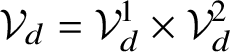 ${\mathcal V}_d={\mathcal V}_d^1\times {\mathcal V}_d^2$
it follows that
${\mathcal V}_d={\mathcal V}_d^1\times {\mathcal V}_d^2$
it follows that
 $$ \begin{align*} {\partial}_{{\mathrm{y}}^1}^*f\cdot {\partial}_{{\mathrm{y}}}f\cdot {\mathcal V}_d={\partial}_{{\mathrm{y}}^1}^*f\cdot {\partial}_{{\mathrm{y}}^1}f\cdot {\mathcal V}_d^1 +{\partial}_{{\mathrm{y}}^1}^*f\cdot {\partial}_{{\mathrm{y}}^2}f\cdot {\mathcal V}_d^2=g\cdot {\mathcal V}_d^1+{\partial}_{{\mathrm{y}}^1}^*f\cdot {\partial}_{{\mathrm{y}}^2}f\cdot {\mathcal V}_d^2. \end{align*} $$
Therefore, the membership
 $f(z)\in {\partial }_{\mathrm {y}}f(z)\cdot {\mathcal V}_d$
is equivalent to saying that the remainder of the componentwise division of
$f(z)\in {\partial }_{\mathrm {y}}f(z)\cdot {\mathcal V}_d$
is equivalent to saying that the remainder of the componentwise division of
 ${\partial }_{\mathrm {y}^1}^*f(z)\cdot f(z)$
by
${\partial }_{\mathrm {y}^1}^*f(z)\cdot f(z)$
by
 $g(z)\cdot {\mathcal V}_d^1$
belongs to the image of
$g(z)\cdot {\mathcal V}_d^1$
belongs to the image of
 ${\partial }_{\mathrm {y}^1}^*f(z)\cdot {\partial }_{\mathrm {y}^2}f(z)\cdot {\mathcal V}_d^2$
in the factor module
${\partial }_{\mathrm {y}^1}^*f(z)\cdot {\partial }_{\mathrm {y}^2}f(z)\cdot {\mathcal V}_d^2$
in the factor module
 $\mathcal A_{\circ }^k/g(z)\cdot {\mathcal V}_d^1$
. But this quotient is a finite-dimensional
$\mathcal A_{\circ }^k/g(z)\cdot {\mathcal V}_d^1$
. But this quotient is a finite-dimensional
 $\mathbf {k}$
-vector space, so the membership defines by Theorem 3.4 (b) a Zariski closed subset
$\mathbf {k}$
-vector space, so the membership defines by Theorem 3.4 (b) a Zariski closed subset
 ${\mathcal Z}_d^*$
of
${\mathcal Z}_d^*$
of
 ${\mathcal Z}_d$
.
${\mathcal Z}_d$
.
Remarks 6.2. (a) It is in general not true that the fibrations
 $\tau _d:{\mathcal {W}}_d\rightarrow {\mathcal Z}_d^*$
and
$\tau _d:{\mathcal {W}}_d\rightarrow {\mathcal Z}_d^*$
and
 $\pi _d:{\mathcal Y}_d\rightarrow {\mathcal Z}_d^*$
are trivial or textile locally trivial. In fact, the dimension of the fibres
$\pi _d:{\mathcal Y}_d\rightarrow {\mathcal Z}_d^*$
are trivial or textile locally trivial. In fact, the dimension of the fibres
 ${\mathcal {W}}_{d,z}$
may vary with z, since the equation
${\mathcal {W}}_{d,z}$
may vary with z, since the equation
 $f(z)+{\partial }_yf(z)\cdot v=0$
defining
$f(z)+{\partial }_yf(z)\cdot v=0$
defining
 ${\mathcal {W}}_{d,z}$
has to be solved for
${\mathcal {W}}_{d,z}$
has to be solved for
 $v=v(\mathrm {t})$
inside
$v=v(\mathrm {t})$
inside
 $\mathcal A_{\circ }^m$
(recall here that the dependence of the series on the variable
$\mathcal A_{\circ }^m$
(recall here that the dependence of the series on the variable
 $\mathrm {t}$
is not marked notationally). This is only possible for those z for which
$\mathrm {t}$
is not marked notationally). This is only possible for those z for which
 $f(z)$
belongs to the
$f(z)$
belongs to the
 $\mathcal A_{\circ }$
-module generated by the vectors
$\mathcal A_{\circ }$
-module generated by the vectors
 ${\partial }_{\mathrm {y}_i}f(z)$
.
${\partial }_{\mathrm {y}_i}f(z)$
.
The statement of the fibration theorem holds under the more general assumption that f admits an arbitrary division module
 ${\mathcal G}$
(and not just one of the form described in Proposition 4.3 and Remark 5.6(a)). The sets
${\mathcal G}$
(and not just one of the form described in Proposition 4.3 and Remark 5.6(a)). The sets
 ${\mathcal S}_{\mathbf {d}}$
,
${\mathcal S}_{\mathbf {d}}$
,
 ${\mathcal V}_{\mathbf {d}}$
,
${\mathcal V}_{\mathbf {d}}$
,
 ${\mathcal R}_{\mathbf {d}}$
and
${\mathcal R}_{\mathbf {d}}$
and
 ${\mathcal Z}_{\mathbf {d}}$
, with
${\mathcal Z}_{\mathbf {d}}$
, with
 $\mathbf {d}=(d_1,\ldots ,d_m)\in {\mathbb N}^m$
, then have to be defined as in the linearisation theorem 5.5. In the factorisation theorem 7.1 it will be shown that there exists a choice of a division module
$\mathbf {d}=(d_1,\ldots ,d_m)\in {\mathbb N}^m$
, then have to be defined as in the linearisation theorem 5.5. In the factorisation theorem 7.1 it will be shown that there exists a choice of a division module
 ${\mathcal G}$
of f such that the fibrations
${\mathcal G}$
of f such that the fibrations
 $\tau _d$
and
$\tau _d$
and
 $\pi _d$
actually become trivial.
$\pi _d$
actually become trivial.
(b) The quasi-affine variety
 ${\mathcal Z}_d^*$
appears implicitly in the proof of the approximation theorem [Reference ArtinAr1, Reference PłoskiPł]: it corresponds to the set of approximate solutions of the equation
${\mathcal Z}_d^*$
appears implicitly in the proof of the approximation theorem [Reference ArtinAr1, Reference PłoskiPł]: it corresponds to the set of approximate solutions of the equation
 $f(\mathrm {y})=0$
modulo the square of the minor g.
$f(\mathrm {y})=0$
modulo the square of the minor g.
(c) The theorem gives no statement about the complement
 ${\mathcal Y}_{\infty }={\mathcal Y}_{\infty }(f)={\mathcal Y}(f)\setminus \bigcup _{d\in {\mathbb N}} {\mathcal Y}_d(f)$
of power series vectors y where the minor g vanishes. To describe this set one will have to apply induction on the height of the ideal I generated by
${\mathcal Y}_{\infty }={\mathcal Y}_{\infty }(f)={\mathcal Y}(f)\setminus \bigcup _{d\in {\mathbb N}} {\mathcal Y}_d(f)$
of power series vectors y where the minor g vanishes. To describe this set one will have to apply induction on the height of the ideal I generated by
 $f_1,\ldots ,f_k$
; see Theorem 8.1 for the details.
$f_1,\ldots ,f_k$
; see Theorem 8.1 for the details.
(d) In the situation of arc spaces (i.e., when f does not depend on
 $\mathrm {t}$
), the sets
$\mathrm {t}$
), the sets
 ${\mathcal Y}_d$
are also known as the contact locus; cf. [Reference de Fernex, Ein and IshiidFEI].
${\mathcal Y}_d$
are also known as the contact locus; cf. [Reference de Fernex, Ein and IshiidFEI].
7 Factorisation theorem
In this and the next section we will prove that every subvariety
 $$ \begin{align*} {\mathcal Y}={\mathcal Y}(I)=\{y\in\mathcal A_{\circ}^m,\, f(y)=0 \text{ for all } f\in I\} \end{align*} $$
defined by some ideal I of
 ${\mathcal B}$
admits a countable stratification into textile locally closed strata which are textile isomorphic to Cartesian products of finite-dimensional varieties with finite free
${\mathcal B}$
admits a countable stratification into textile locally closed strata which are textile isomorphic to Cartesian products of finite-dimensional varieties with finite free
 $\mathcal A_{\circ }$
-modules as stated in Theorem 1.4 from the Introduction. Let
$\mathcal A_{\circ }$
-modules as stated in Theorem 1.4 from the Introduction. Let
 $f_1,\ldots ,f_k$
be generators of I, and set
$f_1,\ldots ,f_k$
be generators of I, and set
 $f=(f_1,\ldots ,f_k) \in {\mathcal B}^k$
.
$f=(f_1,\ldots ,f_k) \in {\mathcal B}^k$
.
The fibration theorem 6.1 provides in the case
 $k\leq m$
and for a chosen
$k\leq m$
and for a chosen
 $(k\times k)$
-minor g of
$(k\times k)$
-minor g of
 ${\partial }_{\mathrm {y}} f$
a stratification of
${\partial }_{\mathrm {y}} f$
a stratification of
 ${\mathcal Y}(f)\setminus {\mathcal Y}(g)$
by strata
${\mathcal Y}(f)\setminus {\mathcal Y}(g)$
by strata
 ${\mathcal Y}_d(f)$
which are linearly fibred. In general, these are not trivial fibrations. We will show in this section that for a smart choice of the division module
${\mathcal Y}_d(f)$
which are linearly fibred. In general, these are not trivial fibrations. We will show in this section that for a smart choice of the division module
 ${\mathcal G}$
of f the fibrations will indeed be trivial; that is, each
${\mathcal G}$
of f the fibrations will indeed be trivial; that is, each
 ${\mathcal Y}_d(f)$
is textile isomorphic to a Cartesian product. This choice of
${\mathcal Y}_d(f)$
is textile isomorphic to a Cartesian product. This choice of
 ${\mathcal G}$
has been used, for instance, by Płoski for proving his parametrisation theorem [Reference PłoskiPł] and also by many other authors; see, for example, [Reference Denef and LoeserDL, Reference Grinberg and KazhdanGK, Reference DrinfeldDr]. The precise statement is as follows.
${\mathcal G}$
has been used, for instance, by Płoski for proving his parametrisation theorem [Reference PłoskiPł] and also by many other authors; see, for example, [Reference Denef and LoeserDL, Reference Grinberg and KazhdanGK, Reference DrinfeldDr]. The precise statement is as follows.
Theorem 7.1. Cartesian factorisation of arquile varieties
Let
 $I\subset {\mathcal B}$
be an ideal generated by series
$I\subset {\mathcal B}$
be an ideal generated by series
 $f_1,\ldots ,f_k$
in
$f_1,\ldots ,f_k$
in
 $\mathrm {t}$
and
$\mathrm {t}$
and
 $\mathrm {y}$
for which there exists a
$\mathrm {y}$
for which there exists a
 $(k\times k)$
-minor g of the relative Jacobian matrix
$(k\times k)$
-minor g of the relative Jacobian matrix
 ${\partial }_{\mathrm {y}}f$
of
${\partial }_{\mathrm {y}}f$
of
 $f=(f_1,\ldots ,f_k)$
which does not vanish identically. Let
$f=(f_1,\ldots ,f_k)$
which does not vanish identically. Let
 $$ \begin{align*} {\mathcal Y}={\mathcal Y}(I)=\{y\in\mathcal A_{\circ}^m,\, f(y)=0\}\subset\mathcal A_{\circ}^m \end{align*} $$
be the arquile variety defined by I in
 $\mathcal A_{\circ }^m$
. Write
$\mathcal A_{\circ }^m$
. Write
 ${\mathcal Y}$
as the disjoint union
${\mathcal Y}$
as the disjoint union
 $$ \begin{align*} {\mathcal Y}=\bigcup_{d\in{\mathbb N}\cup\{\infty\}} {\mathcal Y}_d \end{align*} $$
of textile locally closed subsets, where
 $$ \begin{align*} {\mathcal Y}_d=\{y\in{\mathcal Y},\, g(y)\neq 0,\, \mbox{ord}\, g(y)=d\} \end{align*} $$
for
 $d\in {\mathbb N}$
and where
$d\in {\mathbb N}$
and where
 $$ \begin{align*} {\mathcal Y}_{\infty}=\{y\in{\mathcal Y},\, g(y)=0\}. \end{align*} $$
Then, for
 $d\in {\mathbb N}$
, the strata
$d\in {\mathbb N}$
, the strata
 ${\mathcal Y}_d$
are textile isomorphic (and hence also
${\mathcal Y}_d$
are textile isomorphic (and hence also
 $\mathrm {t}$
-adically homeomorphic) over a Zariski locally closed subset
$\mathrm {t}$
-adically homeomorphic) over a Zariski locally closed subset
 ${\mathcal Z}_d^*$
of
${\mathcal Z}_d^*$
of
 $\mathbb A_{\mathbf {k}}^{d(2m-k)}$
to the Cartesian product of
$\mathbb A_{\mathbf {k}}^{d(2m-k)}$
to the Cartesian product of
 ${\mathcal Z}_d^*$
with a free
${\mathcal Z}_d^*$
with a free
 $\mathcal A_{\circ }$
-module of rank
$\mathcal A_{\circ }$
-module of rank
 $m-k$
,
$m-k$
,

Remarks 7.2. (a) This result specifies the assertions of the structure theorem 1.4 from the Introduction.
(b) For
 $d\in {\mathbb N}$
, the strata
$d\in {\mathbb N}$
, the strata
 ${\mathcal Y}_d$
are textile locally closed and
${\mathcal Y}_d$
are textile locally closed and
 $\mathrm {t}$
-adically open in
$\mathrm {t}$
-adically open in
 $\mathcal A_{\circ }^m$
and textile cofinite locally closed in
$\mathcal A_{\circ }^m$
and textile cofinite locally closed in
 ${\mathcal Y}$
.
${\mathcal Y}$
.
(c) The stratum
 ${\mathcal Y}_{\infty }$
is arquile closed in
${\mathcal Y}_{\infty }$
is arquile closed in
 ${\mathcal Y}$
and defined in
${\mathcal Y}$
and defined in
 $\mathcal A_{\circ }^m$
by the ideal
$\mathcal A_{\circ }^m$
by the ideal
 $I+\langle g\rangle $
. If I is prime of height r and
$I+\langle g\rangle $
. If I is prime of height r and
 $g\not \in I$
, this ideal has height
$g\not \in I$
, this ideal has height
 $r+1$
and can therefore be submitted to induction to find its respective stratification; see Theorem 8.1.
$r+1$
and can therefore be submitted to induction to find its respective stratification; see Theorem 8.1.
(d) The Zariski locally closed subset
 ${\mathcal Z}_d^*$
of
${\mathcal Z}_d^*$
of
 $\mathbb A_{\mathbf {k}}^{d(2m-k)}$
is constructed as follows. We may assume that g is the
$\mathbb A_{\mathbf {k}}^{d(2m-k)}$
is constructed as follows. We may assume that g is the
 $(k\times k)$
-minor defined by the first k columns of
$(k\times k)$
-minor defined by the first k columns of
 ${\partial }_{\mathrm {y}} f$
. Consider the
${\partial }_{\mathrm {y}} f$
. Consider the
 $\mathcal B_{\circ }$
-submodule
$\mathcal B_{\circ }$
-submodule
 $$ \begin{align*} {\mathcal G}=g\cdot\mathcal B_{\circ}^k\times g^2\cdot\mathcal B_{\circ}^{m-k} \end{align*} $$
of
 $\mathcal B_{\circ }^m$
. Proposition 4.3 ensures that
$\mathcal B_{\circ }^m$
. Proposition 4.3 ensures that
 ${\mathcal G}$
is a division module for f; cf. Definition 4.1. For
${\mathcal G}$
is a division module for f; cf. Definition 4.1. For
 $d\in {\mathbb N}$
set
$d\in {\mathbb N}$
set
 $$ \begin{align*} {\mathcal S}_d=\{y\in \mathcal A_{\circ}^m,\, g(y)\neq 0,\, \text { ord}\, g(y)=d\}. \end{align*} $$
The evaluation
 ${\mathcal G}(y)$
does not depend on the choice of
${\mathcal G}(y)$
does not depend on the choice of
 $y\in {\mathcal S}_d$
and equals
$y\in {\mathcal S}_d$
and equals
 $$ \begin{align*} {\mathcal V}_d={\mathcal G}(y)={\mathrm{t}}^d\cdot\mathcal A_{\circ}^k\times {\mathrm{t}}^{2d}\cdot\mathcal A_{\circ}^{m-k}\subset \mathcal A_{\circ}^m. \end{align*} $$
We let
 ${\mathcal R}_d\cong \mathbb A_{\mathbf {k}}^{d(2m-k)}$
denote the direct complement of
${\mathcal R}_d\cong \mathbb A_{\mathbf {k}}^{d(2m-k)}$
denote the direct complement of
 ${\mathcal V}_d$
as in Theorem 5.4, consisting of vectors in
${\mathcal V}_d$
as in Theorem 5.4, consisting of vectors in
 $\mathcal A_{\circ }^m$
whose first k components are polynomials of degree
$\mathcal A_{\circ }^m$
whose first k components are polynomials of degree
 $\leq d$
and whose last
$\leq d$
and whose last
 $m-k$
components are polynomials of degree
$m-k$
components are polynomials of degree
 $\leq 2d$
. Set
$\leq 2d$
. Set
 ${\mathcal Z}_d={\mathcal S}_d\cap {\mathcal R}_d$
and define
${\mathcal Z}_d={\mathcal S}_d\cap {\mathcal R}_d$
and define
 $$ \begin{align*} {\mathcal Z}_d^*=\{z\in{\mathcal Z}_d,\,f(z)\in {\partial}_{{\mathrm{y}}}f(z)\cdot {\mathcal V}_d\}. \end{align*} $$
By assertion (c) of Theorem 6.1, this set is Zariski locally closed in affine space
 $\mathbb A_{\mathbf {k}}^{d(2m-k)}$
.
$\mathbb A_{\mathbf {k}}^{d(2m-k)}$
.
(e) A suitable isomorphism
 $\Phi _d:{\mathcal Y}_d\rightarrow {\mathcal Z}_d^*\times \mathcal A_{\circ }^{m-k}$
is given by the restriction to
$\Phi _d:{\mathcal Y}_d\rightarrow {\mathcal Z}_d^*\times \mathcal A_{\circ }^{m-k}$
is given by the restriction to
 ${\mathcal Y}_d$
of the composition
${\mathcal Y}_d$
of the composition
 $\lambda _d\circ \varphi _d\circ \psi _d$
of the map
$\lambda _d\circ \varphi _d\circ \psi _d$
of the map
 $$ \begin{align*} \varphi_d\circ\psi_d:{\mathcal S}_d\rightarrow {\mathcal Z}_d\times {\mathcal V}_d, \end{align*} $$
 $$ \begin{align*} y=v+z=\Delta(z)\cdot a+z\rightarrow (z,\Delta_g(z)\cdot (a+p(z,a))), \end{align*} $$
defined by the diagonal matrix
 $\Delta =\mathrm {diag}(g,\ldots ,g,g^2,\ldots ,g^2)$
and the power series vector p as in Proposition 5.2 and Theorem 5.4 with the map
$\Delta =\mathrm {diag}(g,\ldots ,g,g^2,\ldots ,g^2)$
and the power series vector p as in Proposition 5.2 and Theorem 5.4 with the map
 $$ \begin{align*} \lambda_d: {\mathcal Z}_d\times{\mathcal V}_d\rightarrow {\mathcal Z}_d\times \mathcal A_{\circ}^k\times\mathcal A_{\circ}^{m-k}, \end{align*} $$
 $$ \begin{align*} (z,v)=(g(z)\cdot a_1, g(z)^2\cdot a_2,z)\rightarrow (z, a_1-{\partial}^*_{{\mathrm{y}}^1}f(z)\cdot {\partial}_{{\mathrm{y}}^2}f(z) \cdot a_2,a_2), \end{align*} $$
where
 $a=(a_1,a_2)$
and
$a=(a_1,a_2)$
and
 $\mathrm {y}=(\mathrm {y}^1,\mathrm {y}^2)$
denote the decompositions of a and
$\mathrm {y}=(\mathrm {y}^1,\mathrm {y}^2)$
denote the decompositions of a and
 $\mathrm {y}$
into the first k and last
$\mathrm {y}$
into the first k and last
 $m-k$
components and where
$m-k$
components and where
 ${\partial }^*_{\mathrm {y}^1}f$
is the adjoint matrix of
${\partial }^*_{\mathrm {y}^1}f$
is the adjoint matrix of
 ${\partial }_{\mathrm {y}^1}f$
.
${\partial }_{\mathrm {y}^1}f$
.
(f) As the minor g varies, the sets
 ${\mathcal Y}_d$
will cover the entire arq.regular locus of
${\mathcal Y}_d$
will cover the entire arq.regular locus of
 ${\mathcal Y}$
; see the next section.
${\mathcal Y}$
; see the next section.
Proof. All constructions and arguments below will be compatible with the restrictions to the convergent or algebraic power series setting. The set
 ${\mathcal Y}_d$
equals the intersection
${\mathcal Y}_d$
equals the intersection
 ${\mathcal Y}\cap {\mathcal S}_d$
. In Theorem 6.1 it was shown that
${\mathcal Y}\cap {\mathcal S}_d$
. In Theorem 6.1 it was shown that
 $ {\mathcal Y}_d$
is textile isomorphic over
$ {\mathcal Y}_d$
is textile isomorphic over
 ${\mathcal Z}_d^*$
to
${\mathcal Z}_d^*$
to
 $$ \begin{align*} {\mathcal{W}}_d=\{(z,v)\in {\mathcal Z}_d\times{\mathcal V}_d,\, f(z)+ {\partial}_{{\mathrm{y}}}f(z)\cdot v=0\} \end{align*} $$
over
 ${\mathcal Z}_d^*$
. The projection
${\mathcal Z}_d^*$
. The projection
 $\tau _d: {\mathcal {W}}_d\rightarrow {\mathcal Z}_d^*,\, (z,v)\rightarrow z$
is by Theorem 6.1 a fibration with fibres
$\tau _d: {\mathcal {W}}_d\rightarrow {\mathcal Z}_d^*,\, (z,v)\rightarrow z$
is by Theorem 6.1 a fibration with fibres
 ${\mathcal {W}}_{d,z}$
which are affine
${\mathcal {W}}_{d,z}$
which are affine
 $\mathcal A_{\circ }$
-modules. We will show that this fibration is trivial for our specific choice
$\mathcal A_{\circ }$
-modules. We will show that this fibration is trivial for our specific choice
 $$ \begin{align*} {\mathcal G}=g \cdot\mathcal B_{\circ}^k\times g^2\cdot\mathcal B_{\circ}^{m-k} \end{align*} $$
of the division module
 ${\mathcal G}$
. To this end, we will construct a textile isomorphism
${\mathcal G}$
. To this end, we will construct a textile isomorphism
 ${\mathcal {W}}_d\rightarrow {\mathcal Z}_d^*\times \mathcal A_{\circ }^{m-k}$
over
${\mathcal {W}}_d\rightarrow {\mathcal Z}_d^*\times \mathcal A_{\circ }^{m-k}$
over
 ${\mathcal Z}_d^*$
.
${\mathcal Z}_d^*$
.
Set
 $\mathrm {y}^1=(\mathrm {y}_1,\ldots ,\mathrm {y}_k)$
and
$\mathrm {y}^1=(\mathrm {y}_1,\ldots ,\mathrm {y}_k)$
and
 $\mathrm {y}^2=(\mathrm {y}_{k+1},\ldots ,\mathrm {y}_m)$
. For
$\mathrm {y}^2=(\mathrm {y}_{k+1},\ldots ,\mathrm {y}_m)$
. For
 $z\in {\mathcal Z}_d$
, the evaluation
$z\in {\mathcal Z}_d$
, the evaluation
 $g(z)$
of the minor g of the submatrix
$g(z)$
of the minor g of the submatrix
 ${\partial }_{\mathrm {y}^1}f(z)$
is nonzero, and therefore the linear map
${\partial }_{\mathrm {y}^1}f(z)$
is nonzero, and therefore the linear map
 $\mathcal A_{\circ }^k\rightarrow \mathcal A_{\circ }^k$
induced by the adjoint matrix
$\mathcal A_{\circ }^k\rightarrow \mathcal A_{\circ }^k$
induced by the adjoint matrix
 ${\partial }^*_{\mathrm {y}^1}f$
of
${\partial }^*_{\mathrm {y}^1}f$
of
 ${\partial }_{\mathrm {y}^1}f$
is injective. By multiplying the system of equations
${\partial }_{\mathrm {y}^1}f$
is injective. By multiplying the system of equations
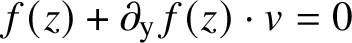 $f(z)+{\partial }_{\mathrm {y}}f(z)\cdot v=0$
from the left with
$f(z)+{\partial }_{\mathrm {y}}f(z)\cdot v=0$
from the left with
 ${\partial }^*_{\mathrm {y}^1}f$
, we hence obtain the equivalent system of equations
${\partial }^*_{\mathrm {y}^1}f$
, we hence obtain the equivalent system of equations
 $$ \begin{align*} {\partial}^*_{{\mathrm{y}}^1}f(z)\cdot f(z)+{\partial}^*_{{\mathrm{y}}^1}f(z)\cdot {\partial}_{{\mathrm{y}}}f(z)\cdot v=0. \end{align*} $$
For
 $z\in {\mathcal Z}_d^*$
and
$z\in {\mathcal Z}_d^*$
and
 $v\in {\mathcal V}_d={\mathcal G}(z)$
, write
$v\in {\mathcal V}_d={\mathcal G}(z)$
, write
 $v=(g(z)\cdot a_1,g(z)^2\cdot a_2)$
with
$v=(g(z)\cdot a_1,g(z)^2\cdot a_2)$
with
 $a_1\in \mathcal A_{\circ }^k$
and
$a_1\in \mathcal A_{\circ }^k$
and
 $a_2\in \mathcal A_{\circ }^{m-k}$
. As
$a_2\in \mathcal A_{\circ }^{m-k}$
. As
 ${\partial }^*_{\mathrm {y}^1}f\cdot {\partial }_{\mathrm {y}^1}f=g\cdot {1\!\! 1}_k$
, the previous system can be rewritten as
${\partial }^*_{\mathrm {y}^1}f\cdot {\partial }_{\mathrm {y}^1}f=g\cdot {1\!\! 1}_k$
, the previous system can be rewritten as
 $$ \begin{align*} {\partial}^*_{{\mathrm{y}}^1}f(z)\cdot f(z)+g(z)^2 \cdot a_1+{\partial}^*_{{\mathrm{y}}^1}f(z)\cdot {\partial}_{{\mathrm{y}}^2}f(z)\cdot g(z)^2 \cdot a_2=0, \end{align*} $$
say,
 $$ \begin{align*} {\partial}^*_{{\mathrm{y}}^1}f(z)\cdot f(z)+ g(z)^2 \cdot [a_1+{\partial}^*_{{\mathrm{y}}^1}f(z)\cdot {\partial}_{{\mathrm{y}}^2}f(z) \cdot a_2]=0. \end{align*} $$
This shows that
 ${\mathcal Z}_d^*$
can equally be defined as
${\mathcal Z}_d^*$
can equally be defined as
 $$ \begin{align*} {\mathcal Z}_d^*=\{z\in{\mathcal Z}_d,\, {\partial}^*_{{\mathrm{y}}^1}f(z)\cdot f(z)\in\langle g(z)^2\rangle\cdot\mathcal A_{\circ}^k\}. \end{align*} $$
Consider now for each
 $z\in {\mathcal Z}_d^*$
the isomorphism
$z\in {\mathcal Z}_d^*$
the isomorphism
 $$ \begin{align*} \lambda_{d,z}: {\mathcal V}_d\rightarrow \mathcal A_{\circ}^k\times\mathcal A_{\circ}^{m-k}, \end{align*} $$
 $$ \begin{align*} v=(g(z)\cdot a_1,g(z)^2\cdot a_2)\rightarrow (a_1-{\partial}^*_{{\mathrm{y}}^1}f(z)\cdot {\partial}_{{\mathrm{y}}^2}f(z) \cdot a_2, a_2). \end{align*} $$
The preceding computations show that the fibres
 ${\mathcal {W}}_{d,z}$
are sent by
${\mathcal {W}}_{d,z}$
are sent by
 $\lambda _{d,z}$
to the solutions
$\lambda _{d,z}$
to the solutions
 $a=(a_1,a_2)\in \mathcal A_{\circ }^r \times \mathcal A_{\circ }^{m-k}$
of the system of equations
$a=(a_1,a_2)\in \mathcal A_{\circ }^r \times \mathcal A_{\circ }^{m-k}$
of the system of equations
 $$ \begin{align*} {\partial}^*_{{\mathrm{y}}^1}f(z)\cdot f(z)+ g(z)\cdot g(z) \cdot a_1=0. \end{align*} $$
As
 ${\partial }^*_{\mathrm {y}^1}f(z)\cdot f(z)\in g(z)\cdot g(z)\cdot \mathcal A_{\circ }^k$
for
${\partial }^*_{\mathrm {y}^1}f(z)\cdot f(z)\in g(z)\cdot g(z)\cdot \mathcal A_{\circ }^k$
for
 $z\in {\mathcal Z}_d^*$
, these solutions are of the form
$z\in {\mathcal Z}_d^*$
, these solutions are of the form
 $$ \begin{align*} (a_1,a_2)=(-g(z)^{-2}\cdot {\partial}^*_{{\mathrm{y}}^1}f(z)\cdot f(z),a_2), \end{align*} $$
with arbitrary
 $a_2\in \mathcal A_{\circ }^{m-k}$
. It follows that the map
$a_2\in \mathcal A_{\circ }^{m-k}$
. It follows that the map
 $$ \begin{align*} \lambda_d: {\mathcal{W}}_d\rightarrow {\mathcal Z}_d^*\times\mathcal A_{\circ}^{m-k},\, (z,v)\rightarrow(z,\lambda_{d,z}(v)) \end{align*} $$
is a textile isomorphism over
 ${\mathcal Z}_d^*$
. Composing
${\mathcal Z}_d^*$
. Composing
 $\lambda _d$
with
$\lambda _d$
with
 $\varphi _d\circ \psi _d:{\mathcal S}_d\rightarrow {\mathcal Z}_d\rightarrow {\mathcal V}_d$
as in Proposition 5.2 gives the required isomorphism
$\varphi _d\circ \psi _d:{\mathcal S}_d\rightarrow {\mathcal Z}_d\rightarrow {\mathcal V}_d$
as in Proposition 5.2 gives the required isomorphism
 $\Phi _d=\lambda _d\circ \varphi _d\circ \psi _d$
for
$\Phi _d=\lambda _d\circ \varphi _d\circ \psi _d$
for
 ${\mathcal Y}_d$
. This concludes the proof of the factorisation theorem.
${\mathcal Y}_d$
. This concludes the proof of the factorisation theorem.
8 Partition of arquile varieties
In this section we indicate how to decompose and stratify an arbitrary arquile subvariety
 ${\mathcal Y}(I)$
of
${\mathcal Y}(I)$
of
 $\mathcal A_{\circ }^m$
such that on each stratum the factorisation theorem 7.1 can be applied. This, in turn, will then establish the structure theorem 1.4 for arquile varieties from the introduction.
$\mathcal A_{\circ }^m$
such that on each stratum the factorisation theorem 7.1 can be applied. This, in turn, will then establish the structure theorem 1.4 for arquile varieties from the introduction.
So let
 $I\subset {\mathcal B}$
be an ideal, and let
$I\subset {\mathcal B}$
be an ideal, and let
 ${\mathcal Y}={\mathcal Y}(I)$
be its associated zeroset in
${\mathcal Y}={\mathcal Y}(I)$
be its associated zeroset in
 $\mathcal A_{\circ }^m$
. Without loss of generality, we may assume that I is saturated; that is, that I equals the ideal
$\mathcal A_{\circ }^m$
. Without loss of generality, we may assume that I is saturated; that is, that I equals the ideal
 $I_{{\mathcal Y}(I)}$
as defined in Section 2. In particular, I will be radical. Let
$I_{{\mathcal Y}(I)}$
as defined in Section 2. In particular, I will be radical. Let
 $$ \begin{align*} I=I_1\cap\ldots\cap I_s \end{align*} $$
be the irredundant prime decomposition of I, with
 $I_j\subset {\mathcal B}$
prime. By Proposition 2.3, all ideals
$I_j\subset {\mathcal B}$
prime. By Proposition 2.3, all ideals
 $I_j$
are again saturated. We get
$I_j$
are again saturated. We get
 $$ \begin{align*} {\mathcal Y}(I)={\mathcal Y}(I_1)\cup\ldots\cup {\mathcal Y}(I_s), \end{align*} $$
and each
 ${\mathcal Y}(I_j)$
is arquile closed in
${\mathcal Y}(I_j)$
is arquile closed in
 ${\mathcal Y}$
. Recall that
${\mathcal Y}$
. Recall that
 $\mathrm {Arq.Reg}({\mathcal Y})$
denotes the arq.regular locus of points y of
$\mathrm {Arq.Reg}({\mathcal Y})$
denotes the arq.regular locus of points y of
 ${\mathcal Y}$
for which
${\mathcal Y}$
for which
 $({\mathcal B}/I)_{{\mathcal P}_y}$
is a regular local ring, where
$({\mathcal B}/I)_{{\mathcal P}_y}$
is a regular local ring, where
 ${\mathcal P}_y\subset {\mathcal B}$
is the prime ideal of relations among the components of y. This locus is arquile open in
${\mathcal P}_y\subset {\mathcal B}$
is the prime ideal of relations among the components of y. This locus is arquile open in
 ${\mathcal Y}$
. For
${\mathcal Y}$
. For
 $y\in \mathrm {Arq.Reg}({\mathcal Y})$
, let
$y\in \mathrm {Arq.Reg}({\mathcal Y})$
, let
 $r_y$
be the height of the ideal
$r_y$
be the height of the ideal
 $I\cdot {\mathcal B}_{{\mathcal P}_y}$
. For
$I\cdot {\mathcal B}_{{\mathcal P}_y}$
. For
 $r\in {\mathbb N}$
, denote by
$r\in {\mathbb N}$
, denote by
 ${\mathcal Y}_r$
the arquile locally closed subset of
${\mathcal Y}_r$
the arquile locally closed subset of
 ${\mathcal Y}$
of points
${\mathcal Y}$
of points
 $y\in \mathrm {Arq.Reg}({\mathcal Y})$
with
$y\in \mathrm {Arq.Reg}({\mathcal Y})$
with
 $r_y=r$
. By part (c) of Theorem 2.6, each
$r_y=r$
. By part (c) of Theorem 2.6, each
 ${\mathcal Y}_r$
is covered by finitely many arquile open subsets of the form
${\mathcal Y}_r$
is covered by finitely many arquile open subsets of the form
 ${\mathcal Y}(f)\setminus {\mathcal Y}(g)$
, where
${\mathcal Y}(f)\setminus {\mathcal Y}(g)$
, where
 $f=(f_1,\ldots ,f_r)$
is a vector of elements in I and g is a suitable
$f=(f_1,\ldots ,f_r)$
is a vector of elements in I and g is a suitable
 $(r\times r)$
-minor of the relative Jacobian matrix
$(r\times r)$
-minor of the relative Jacobian matrix
 ${\partial }_{\mathrm {y}} f$
of f. Varying r then yields an arquile and
${\partial }_{\mathrm {y}} f$
of f. Varying r then yields an arquile and
 $\mathrm {t}$
-adically open covering of
$\mathrm {t}$
-adically open covering of
 $\mathrm {Arq.Reg}({\mathcal Y})$
by such sets.
$\mathrm {Arq.Reg}({\mathcal Y})$
by such sets.
By part (e) of Theorem 2.6, the arq.singular locus
 $\mathrm {Arq.Sing}({\mathcal Y})$
is an arquile closed proper subset of
$\mathrm {Arq.Sing}({\mathcal Y})$
is an arquile closed proper subset of
 ${\mathcal Y}$
. As
${\mathcal Y}$
. As
 $\mathcal A_{\circ }^m$
is Noetherian with respect to the arquile topology, we may apply induction to stratify
$\mathcal A_{\circ }^m$
is Noetherian with respect to the arquile topology, we may apply induction to stratify
 $\mathrm {Arq.Sing}({\mathcal Y})$
suitably, starting again with its arq.regular locus
$\mathrm {Arq.Sing}({\mathcal Y})$
suitably, starting again with its arq.regular locus
 $\mathrm {Arq.Reg}(\mathrm {Arq.Sing}({\mathcal Y}))$
and then passing on to its arq.singular locus
$\mathrm {Arq.Reg}(\mathrm {Arq.Sing}({\mathcal Y}))$
and then passing on to its arq.singular locus
 $\mathrm {Arq.Sing}(\mathrm {Arq.Sing}({\mathcal Y}))$
. Note that the strata will now be just arquile locally closed in
$\mathrm {Arq.Sing}(\mathrm {Arq.Sing}({\mathcal Y}))$
. Note that the strata will now be just arquile locally closed in
 ${\mathcal Y}$
. Putting all of this together then gives the following.
${\mathcal Y}$
. Putting all of this together then gives the following.
Theorem 8.1. Partition of arquile varieties
Every arquile subvariety
 ${\mathcal Y}={\mathcal Y}(I)$
of
${\mathcal Y}={\mathcal Y}(I)$
of
 $\mathcal A_{\circ }^m$
admits a finite stratification
$\mathcal A_{\circ }^m$
admits a finite stratification
 ${\mathcal Y}=\bigsqcup \, {\mathcal Y}_i$
into arquile locally closed subsets
${\mathcal Y}=\bigsqcup \, {\mathcal Y}_i$
into arquile locally closed subsets
 ${\mathcal Y}_i=\mathrm {Arq.Sing}_i({\mathcal Y})\setminus \mathrm {Arq.Sing}_{i+1}({\mathcal Y})$
such that each
${\mathcal Y}_i=\mathrm {Arq.Sing}_i({\mathcal Y})\setminus \mathrm {Arq.Sing}_{i+1}({\mathcal Y})$
such that each
 ${\mathcal Y}_i$
has a finite arquile and
${\mathcal Y}_i$
has a finite arquile and
 $\mathrm {t}$
-adically open covering by sets of the form
$\mathrm {t}$
-adically open covering by sets of the form
 ${\mathcal U}_g={\mathcal Y}(f)\setminus {\mathcal Y}(g)$
, where
${\mathcal U}_g={\mathcal Y}(f)\setminus {\mathcal Y}(g)$
, where
 $f\in {\mathcal B}^k$
is a vector of power series and where g is a minor of the relative Jacobian matrix
$f\in {\mathcal B}^k$
is a vector of power series and where g is a minor of the relative Jacobian matrix
 ${\partial }_{\mathrm {y}} f$
of f of size equal to the height of the ideal of
${\partial }_{\mathrm {y}} f$
of f of size equal to the height of the ideal of
 ${\mathcal B}$
generated by the components of f.
${\mathcal B}$
generated by the components of f.
9 Example
Example 9.1. Let
 ${\mathcal Y}(f)\subset \mathcal A_{\circ }^3$
be the arquile variety given by
${\mathcal Y}(f)\subset \mathcal A_{\circ }^3$
be the arquile variety given by
 $f(\mathrm {y}) = \mathrm {y}_{1}^{2} - \mathrm {y}_{2} \mathrm {y}_{3}$
. Since the parameter
$f(\mathrm {y}) = \mathrm {y}_{1}^{2} - \mathrm {y}_{2} \mathrm {y}_{3}$
. Since the parameter
 $\mathrm {t}$
does not appear in the equation and since f is irreducible, the singular locus equals
$\mathrm {t}$
does not appear in the equation and since f is irreducible, the singular locus equals
 $\mathrm {Arq.Sing}({\mathcal Y}) = {\mathcal Y}(f, \partial _{\mathrm {y}_{1}}f,\partial _{\mathrm {y}_{2}}f,\partial _{\mathrm {y}_{3}}f) =\{(0,0,0)\}$
and the arq.regular part is covered by
$\mathrm {Arq.Sing}({\mathcal Y}) = {\mathcal Y}(f, \partial _{\mathrm {y}_{1}}f,\partial _{\mathrm {y}_{2}}f,\partial _{\mathrm {y}_{3}}f) =\{(0,0,0)\}$
and the arq.regular part is covered by
 ${\mathcal Y}(f) \setminus {\mathcal Y}(\partial _{\mathrm {y}_{i}}f)$
. We fix
${\mathcal Y}(f) \setminus {\mathcal Y}(\partial _{\mathrm {y}_{i}}f)$
. We fix
 $i=1$
, so we consider the set
$i=1$
, so we consider the set
 ${\mathcal Y}(f)\setminus {\mathcal Y}(\mathrm {y}_{1})$
, which we stratify into the sets
${\mathcal Y}(f)\setminus {\mathcal Y}(\mathrm {y}_{1})$
, which we stratify into the sets
 $(d\geq 1)$
 $$ \begin{align*} {\mathcal Y}_{d} = \{y \in {\mathcal Y}(f),\, \text{ord}\, y_{1} = d\}. \end{align*} $$
It is easily seen that
 $$ \begin{align*} {\mathcal Z}_{d} = \left\{ \left(z_{1,d} {\mathrm{t}}^{d}, \sum_{k=1}^{2d} z_{2,k} {\mathrm{t}}^{k}, \sum_{k=1}^{2d} z_{3,k} {\mathrm{t}}^{k}\right),\, z_{1,d}\ \neq 0 \right\}. \end{align*} $$
In the hypersurface case, the defining minor for
 ${\mathcal Z}_{d}$
stems from the derivative
${\mathcal Z}_{d}$
stems from the derivative
 $\partial _{\mathrm {y}_{1}}f$
, whence
$\partial _{\mathrm {y}_{1}}f$
, whence
 $\partial ^{*}_{\mathrm {y}_{1}} f = 1$
. Therefore, the equation for
$\partial ^{*}_{\mathrm {y}_{1}} f = 1$
. Therefore, the equation for
 ${\mathcal Z}_{d}^{*}$
simplifies to
${\mathcal Z}_{d}^{*}$
simplifies to
 $f(z) \equiv 0 \mod \mathrm {t}^{2d + 1}$
, which is equivalent to the system
$f(z) \equiv 0 \mod \mathrm {t}^{2d + 1}$
, which is equivalent to the system
 $$ \begin{align*} z_{1,d} &\neq 0,\\ z_{2,1}z_{3,1} &=0,\\ &\vdots \\ \sum_{j=1}^{2d-1} z_{2,2d-1 - j} z_{3,j} &= 0,\\ z_{1,d}^{2} - \sum_{j=1}^{2d} z_{2,2d - j} z_{3,j} &= 0. \end{align*} $$
By the Cartesian factorisation theorem 7.1,
 ${\mathcal Y}_{d}$
is isomorphic to
${\mathcal Y}_{d}$
is isomorphic to
 ${\mathcal Z}^{*}_{d} \times \mathcal A_{\circ }^{2}$
. An isomorphism
${\mathcal Z}^{*}_{d} \times \mathcal A_{\circ }^{2}$
. An isomorphism
 $$ \begin{align*} \Phi^{-1}_{d} = (\Phi^{-1}_{d,1},\Phi^{-1}_{d,2},\Phi^{-1}_{d,3}) \colon {\mathcal Z}^{*}_{d} \times \mathcal A_{\circ}^{2} \rightarrow {\mathcal Y}_{d} \end{align*} $$
can be explicitly computed and is given by
 $$ \begin{align*} \Phi_{d,1}^{-1}(z_{1},z_{2},z_{3}, a_{2},a_{3}) = z_{1} + {\mathrm{t}}^{d}\cdot(-z_{1,d} + \sqrt{\Xi(z_{1},z_{2},z_{3}, a_{2},a_{3}) }), \end{align*} $$
 $$ \begin{align*} \Phi_{d,2}^{-1}(z_{1},z_{2},z_{3}, a_{2},a_{3}) = z_{2} + {\mathrm{t}}^{2d} a_{2}, \end{align*} $$
 $$ \begin{align*} \Phi_{d,3}^{-1}(z_{1},z_{2},z_{3}, a_{2},a_{3}) = z_{3} + {\mathrm{t}}^{2d}a_{3}, \end{align*} $$
where
 $$ \begin{align*} \Xi(z_{1},z_{2},z_{3}, a_{2},a_{3}) = z_{1,d}^{2} - \frac{z_{1}^2 - z_{2}z_{3}}{{\mathrm{t}}^{2d}} +z_{2}a_{3} + z_{3}a_{2} + {\mathrm{t}}^{2d} a_{2} a_{3}. \end{align*} $$
Here is a short explanation for these formulas. We expand
 $f(z + v) $
into
$f(z + v) $
into
 $ f(z) + \partial _{\mathrm {y}}(f)(z) \cdot v + q(z,v)$
, say
$ f(z) + \partial _{\mathrm {y}}(f)(z) \cdot v + q(z,v)$
, say
 $$ \begin{align*} f(z + v) = (z_{1}^{2} -z_{2}z_{3}) + 2z_{1}v_{1} - z_{2}v_{3} - z_{3}v_{2} + (v_{1}^{2} - v_{2} v_{3} ). \end{align*} $$
Substitute
 $v_{1} = \mathrm {t}^{d} a_{1}, \ v_{2} = \mathrm {t}^{2d}a_{2} ,\ v_{3} = \mathrm {t}^{2d} a_{3}$
. We assume that
$v_{1} = \mathrm {t}^{d} a_{1}, \ v_{2} = \mathrm {t}^{2d}a_{2} ,\ v_{3} = \mathrm {t}^{2d} a_{3}$
. We assume that
 $z \in \mathcal {Z}_{d}^{*}$
, so there exists a series
$z \in \mathcal {Z}_{d}^{*}$
, so there exists a series
 $h_{z}(\mathrm {t}) \in \mathcal A_{\circ }$
such that
$h_{z}(\mathrm {t}) \in \mathcal A_{\circ }$
such that
 $z_{1}^{2} - z_{2}z_{3} = \mathrm {t}^{2d} \cdot h_{z}(t)$
. We want to solve
$z_{1}^{2} - z_{2}z_{3} = \mathrm {t}^{2d} \cdot h_{z}(t)$
. We want to solve
 $f(z + v) = 0$
, which in
$f(z + v) = 0$
, which in
 $\mathrm {a}$
-coordinates takes the form
$\mathrm {a}$
-coordinates takes the form
 $$ \begin{align*} (z_{1}^{2} -z_{2}z_{3}) + 2z_{1}{\mathrm{t}}^{d}a_{1} - z_{2}{\mathrm{t}}^{2d}a_{3} - z_{3}{\mathrm{t}}^{2d}a_{2} + ({\mathrm{t}}^{2d}a_{1}^{2} - {\mathrm{t}}^{2d}a_{2} {\mathrm{t}}^{2d}a_{3} )=0, \end{align*} $$
say
 $$ \begin{align*} {\mathrm{t}}^{2d} \cdot\left( h_{z}({\mathrm{t}}) + 2z_{1,d}a_{1} - z_{2}a_{3} - z_{3}a_{2} + a_{1}^{2} - {\mathrm{t}}^{2d}a_{2} a_{3} \right) = 0. \end{align*} $$
Therefore,
 $$ \begin{align*} a_{1} ={} -z_{1,d} + \sqrt{ z_{1,d}^{2} - \frac{z_{1}^2 - z_{2}z_{3}}{{\mathrm{t}}^{2d}} + z_{2} a_{3} + z_{3}a_{2} + {\mathrm{t}}^{2d} a_{2}a_{3}} \end{align*} $$
as claimed (the square root exists since the order in t of the series is
 $0$
).
$0$
).
10 Deformations
In this section we formulate the analogue of the factorisation theorem 7.1 for the set
 ${\mathcal Y}(f)_S$
of deformations
${\mathcal Y}(f)_S$
of deformations
 $\widetilde y(\mathrm {t})$
of a given power series vector
$\widetilde y(\mathrm {t})$
of a given power series vector
 $y(\mathrm {t})\in {\mathcal Y}(f)\subset \mathcal A_{\circ }^m$
over a base ring S. Considering deformations of y corresponds to working, in a certain sense, locally at y. To establish the Cartesian product structure of the set of deformations it will no longer be necessary to stratify the arquile variety
$y(\mathrm {t})\in {\mathcal Y}(f)\subset \mathcal A_{\circ }^m$
over a base ring S. Considering deformations of y corresponds to working, in a certain sense, locally at y. To establish the Cartesian product structure of the set of deformations it will no longer be necessary to stratify the arquile variety
 ${\mathcal Y}(f)$
, and the partition theorem 8.1 becomes redundant: one can directly prove the factorisation. Taking in particular deformations parametrised by the elements of a test algebra S (a local ring whose maximal ideal is nilpotent), the results of this section contain the factorisation of formal neighbourhoods of arc spaces as proven by Grinberg–Kazhdan and Drinfeld [Reference Grinberg and KazhdanGK, Reference DrinfeldDr, Reference Bruschek and HauserBH, Reference Bourqui and SebagBS1, Reference Bourqui and SebagBS2, Reference BouthierBou].
${\mathcal Y}(f)$
, and the partition theorem 8.1 becomes redundant: one can directly prove the factorisation. Taking in particular deformations parametrised by the elements of a test algebra S (a local ring whose maximal ideal is nilpotent), the results of this section contain the factorisation of formal neighbourhoods of arc spaces as proven by Grinberg–Kazhdan and Drinfeld [Reference Grinberg and KazhdanGK, Reference DrinfeldDr, Reference Bruschek and HauserBH, Reference Bourqui and SebagBS1, Reference Bourqui and SebagBS2, Reference BouthierBou].
We restrict to the case of formal power series and let
 $\mathcal A_{\circ }=\mathbf {k}_{\circ }[[\mathrm {t}]]$
always denote the ring of series without constant term. Similar results as below can be proven in the convergent setting, but the details are more involved and require Banach-space techniques as developed in [Reference Hauser and MüllerHM].
$\mathcal A_{\circ }=\mathbf {k}_{\circ }[[\mathrm {t}]]$
always denote the ring of series without constant term. Similar results as below can be proven in the convergent setting, but the details are more involved and require Banach-space techniques as developed in [Reference Hauser and MüllerHM].
Let S be a local, not necessarily Noetherian ring with maximal ideal
 $M_S$
and residue field
$M_S$
and residue field
 $S/M_S=\mathbf {k}$
embedding into S as a subfield. We shall always assume that S is complete with respect to a filtered topology defined by a decreasing sequence of ideals
$S/M_S=\mathbf {k}$
embedding into S as a subfield. We shall always assume that S is complete with respect to a filtered topology defined by a decreasing sequence of ideals
 $J_k$
with
$J_k$
with
 $J_k\cdot J_{\ell }\subset J_{k+\ell }$
and such that
$J_k\cdot J_{\ell }\subset J_{k+\ell }$
and such that
 $M_S^k\subset J_k$
.
$M_S^k\subset J_k$
.
Denote as in the section on division by
 ${\mathcal A}_{S,\circ }=S_{\circ }[[\mathrm {t}]]$
the ring of formal power series in
${\mathcal A}_{S,\circ }=S_{\circ }[[\mathrm {t}]]$
the ring of formal power series in
 $\mathrm {t}$
with coefficients in S and zero constant term. We shall write
$\mathrm {t}$
with coefficients in S and zero constant term. We shall write
 $\widetilde y(\mathrm {t}) =(\widetilde y_1(\mathrm {t}),\ldots ,\widetilde y_m(\mathrm {t}))$
for power series vectors in
$\widetilde y(\mathrm {t}) =(\widetilde y_1(\mathrm {t}),\ldots ,\widetilde y_m(\mathrm {t}))$
for power series vectors in
 ${\mathcal A}_{S,\circ }^m$
, with coefficient vectors
${\mathcal A}_{S,\circ }^m$
, with coefficient vectors
 $(\widetilde y_{1j},\ldots ,\widetilde y_{mj})$
in
$(\widetilde y_{1j},\ldots ,\widetilde y_{mj})$
in
 $S^m$
of the monomials
$S^m$
of the monomials
 $\mathrm {t}^j$
, for
$\mathrm {t}^j$
, for
 $j\geq 1$
. Their residue classes
$j\geq 1$
. Their residue classes
 $y(\mathrm {t})$
modulo
$y(\mathrm {t})$
modulo
 $M_S$
are power series vectors in
$M_S$
are power series vectors in
 $\mathcal A_{\circ }^m$
, and
$\mathcal A_{\circ }^m$
, and
 $\widetilde y(\mathrm {t})$
is then called a deformation of
$\widetilde y(\mathrm {t})$
is then called a deformation of
 $y(\mathrm {t})$
. We may thus write
$y(\mathrm {t})$
. We may thus write
 $$ \begin{align*} \widetilde y({\mathrm{t}})= y({\mathrm{t}})+\widetilde y\,'({\mathrm{t}}) \end{align*} $$
where
 $\widetilde y\,'(\mathrm {t})\in M_S[[\mathrm {t}]]^m$
is a vector with coefficients in
$\widetilde y\,'(\mathrm {t})\in M_S[[\mathrm {t}]]^m$
is a vector with coefficients in
 $M_S$
, say, a deformation of
$M_S$
, say, a deformation of
 $0\in \mathbf {k}^m$
. The set of all deformations
$0\in \mathbf {k}^m$
. The set of all deformations
 $\widetilde y(\mathrm {t})$
of a vector
$\widetilde y(\mathrm {t})$
of a vector
 $y=y(\mathrm {t})\in \mathcal A_{\circ }^m$
parametrised by S is denoted by
$y=y(\mathrm {t})\in \mathcal A_{\circ }^m$
parametrised by S is denoted by
 $({\mathcal A}_{S,\circ }^m,y)$
, say
$({\mathcal A}_{S,\circ }^m,y)$
, say
 $$ \begin{align*} ({\mathcal A}_{S,\circ}^m,y) = y({\mathrm{t}})+ M_S\cdot {\textbf{k}}[[{\mathrm{t}}]]^m. \end{align*} $$
Let
 $\mathrm {s}_{ij}$
denote countably many variables, for
$\mathrm {s}_{ij}$
denote countably many variables, for
 $1\leq i \leq m$
and
$1\leq i \leq m$
and
 $j\geq 1$
, and let
$j\geq 1$
, and let
 $\mathbf {k}[[\mathrm {s}_{m,\infty }]]$
be the power series ring
$\mathbf {k}[[\mathrm {s}_{m,\infty }]]$
be the power series ring
 $\mathbf {k}[[\mathrm {s}_{ij},\, 1\leq i \leq m,\, j\geq 1]]$
in these variables, with maximal ideal
$\mathbf {k}[[\mathrm {s}_{ij},\, 1\leq i \leq m,\, j\geq 1]]$
in these variables, with maximal ideal
 $(\mathrm {s}_{ij},\, 1\leq i \leq m,\, j\geq 1)$
. For a given vector
$(\mathrm {s}_{ij},\, 1\leq i \leq m,\, j\geq 1)$
. For a given vector
 $y(\mathrm {t})\in \mathcal A_{\circ }^m$
, the vector
$y(\mathrm {t})\in \mathcal A_{\circ }^m$
, the vector
 $\widetilde y(\mathrm {t})=(\widetilde y_1(\mathrm {t}),\ldots ,\widetilde y_m(\mathrm {t}))$
given by
$\widetilde y(\mathrm {t})=(\widetilde y_1(\mathrm {t}),\ldots ,\widetilde y_m(\mathrm {t}))$
given by
 $$ \begin{align*} \widetilde y_i({\mathrm{t}})= y_i({\mathrm{t}})+\sum_{j\geq 1} {\mathrm{s}}_{ij}\cdot {\mathrm{t}}^j \end{align*} $$
defines a universal deformation of
 $y(\mathrm {t})$
, cf. [Reference HauserHa1]: any other deformation of
$y(\mathrm {t})$
, cf. [Reference HauserHa1]: any other deformation of
 $y(\mathrm {t})$
over a ring S is obtained from this one by the evaluation of
$y(\mathrm {t})$
over a ring S is obtained from this one by the evaluation of
 $\mathrm {s}_{ij}$
at elements of
$\mathrm {s}_{ij}$
at elements of
 $M_S$
; that is, by base change.
$M_S$
; that is, by base change.
Let
 ${\mathcal B}$
be defined as in the earlier sections as the space of formal, convergent or algebraic power series in
${\mathcal B}$
be defined as in the earlier sections as the space of formal, convergent or algebraic power series in
 $\mathrm {t}$
and variables
$\mathrm {t}$
and variables
 $\mathrm {y}_1,\ldots ,\mathrm {y}_m$
. Vectors
$\mathrm {y}_1,\ldots ,\mathrm {y}_m$
. Vectors
 $f(\mathrm {t},\mathrm {y})\in {\mathcal B}^k$
with
$f(\mathrm {t},\mathrm {y})\in {\mathcal B}^k$
with
 $f(0)=0$
and with associated arquile map
$f(0)=0$
and with associated arquile map
 $f_{\infty }:\mathcal A_{\circ }^m\rightarrow \mathcal A_{\circ }^k$
define, for every ring S, also a map on
$f_{\infty }:\mathcal A_{\circ }^m\rightarrow \mathcal A_{\circ }^k$
define, for every ring S, also a map on
 ${\mathcal A}_{S,\circ }^m$
,
${\mathcal A}_{S,\circ }^m$
,
 $$ \begin{align*} f_{S,\infty}:{\mathcal A}_{S,\circ}^m\rightarrow {\mathcal A}_{S,\circ}^k,\, \widetilde y({\mathrm{t}})\rightarrow f({\mathrm{t}},\widetilde y({\mathrm{t}})), \end{align*} $$
called the arquile map over S induced by f, and a map
 $$ \begin{align*} (f_{S,\infty},y):({\mathcal A}_{S,\circ}^m,y)\rightarrow ({\mathcal A}_{S,\circ}^k, f_{\infty}(y)),\,\widetilde y({\mathrm{t}})\rightarrow f({\mathrm{t}},\widetilde y({\mathrm{t}})) \end{align*} $$
between the respective sets of deformations of
 $y\in \mathcal A_{\circ }^m$
and
$y\in \mathcal A_{\circ }^m$
and
 $f_{\infty }(y)\in \mathcal A_{\circ }^k$
. For an arquile subvariety
$f_{\infty }(y)\in \mathcal A_{\circ }^k$
. For an arquile subvariety
 ${\mathcal Y}={\mathcal Y}(f)$
of
${\mathcal Y}={\mathcal Y}(f)$
of
 $\mathcal A_{\circ }^m$
defined by a vector
$\mathcal A_{\circ }^m$
defined by a vector
 $f\in {\mathcal B}^k$
, we shall write
$f\in {\mathcal B}^k$
, we shall write
 $$ \begin{align*} ({\mathcal Y}_S,y)=({\mathcal Y}_S(f),y) \end{align*} $$
for the set of deformations
 $\widetilde y$
of y ‘lying in
$\widetilde y$
of y ‘lying in
 ${\mathcal Y}$
’; that is, satisfying
${\mathcal Y}$
’; that is, satisfying
 $f_{S,\infty }(\widetilde y)=0$
. Expanding
$f_{S,\infty }(\widetilde y)=0$
. Expanding
 $f_{S,\infty }(\widetilde y)=f(\mathrm {t},\widetilde y(\mathrm {t}))$
as a power series in
$f_{S,\infty }(\widetilde y)=f(\mathrm {t},\widetilde y(\mathrm {t}))$
as a power series in
 $\mathrm {t}$
one sees that these deformations are defined by setting the coefficients of
$\mathrm {t}$
one sees that these deformations are defined by setting the coefficients of
 $\mathrm {t}^j$
in
$\mathrm {t}^j$
in
 $f(\mathrm {t},\widetilde y(\mathrm {t}))$
equal to
$f(\mathrm {t},\widetilde y(\mathrm {t}))$
equal to
 $0$
for all
$0$
for all
 $j\geq 0$
. This then induces polynomial equations for the coefficients of
$j\geq 0$
. This then induces polynomial equations for the coefficients of
 $\widetilde y$
because the constant term of
$\widetilde y$
because the constant term of
 $\widetilde y$
is assumed to be zero. Taking in particular
$\widetilde y$
is assumed to be zero. Taking in particular
 $S=\mathbf {k}[[\mathrm {s}_{m,\infty }]]$
, we get in this way an ideal
$S=\mathbf {k}[[\mathrm {s}_{m,\infty }]]$
, we get in this way an ideal
 $I({\mathcal Y},y)_{\infty }$
in S of universal polynomials, respectively power series, defining the deformations of y in
$I({\mathcal Y},y)_{\infty }$
in S of universal polynomials, respectively power series, defining the deformations of y in
 ${\mathcal Y}(f)$
over
${\mathcal Y}(f)$
over
 $\mathbf {k}[[\mathrm {s}_{m,\infty }]]$
. We may then identify deformations in
$\mathbf {k}[[\mathrm {s}_{m,\infty }]]$
. We may then identify deformations in
 $({\mathcal Y}_S(f),y)$
with deformations of y in
$({\mathcal Y}_S(f),y)$
with deformations of y in
 ${\mathcal A}_{S'}^m$
parametrised by the factor ring
${\mathcal A}_{S'}^m$
parametrised by the factor ring
 $S'=S/I$
, with
$S'=S/I$
, with
 $I=I({\mathcal Y},y)_{\infty }$
.
$I=I({\mathcal Y},y)_{\infty }$
.
Example 10.1. Let
 $y(\mathrm {t})=(\mathrm {t}^2,\mathrm {t}^3)$
be the canonical solution of
$y(\mathrm {t})=(\mathrm {t}^2,\mathrm {t}^3)$
be the canonical solution of
 $f(\mathrm {y})=\mathrm {y}_1^3-\mathrm {y}_2^2=0$
, and consider a deformation
$f(\mathrm {y})=\mathrm {y}_1^3-\mathrm {y}_2^2=0$
, and consider a deformation
 $\widetilde y(\mathrm {t})=(\mathrm {t}^2+\mathrm {s}_1\mathrm {t},\mathrm {t}^3+\mathrm {s}_2\mathrm {t}^2)$
of
$\widetilde y(\mathrm {t})=(\mathrm {t}^2+\mathrm {s}_1\mathrm {t},\mathrm {t}^3+\mathrm {s}_2\mathrm {t}^2)$
of
 $y(\mathrm {t})$
with
$y(\mathrm {t})$
with
 $S=\mathbf {k}[[\mathrm {s}_1,\mathrm {s}_2]]$
. Then
$S=\mathbf {k}[[\mathrm {s}_1,\mathrm {s}_2]]$
. Then
 $f(\widetilde y(\mathrm {t}))=0$
if and only if
$f(\widetilde y(\mathrm {t}))=0$
if and only if
 $$ \begin{align*} 3{\mathrm{t}}^4{\mathrm{s}}_1{\mathrm{t}}+3{\mathrm{t}}^2{\mathrm{s}}_1^2{\mathrm{t}}^2+{\mathrm{s}}_1^3{\mathrm{t}}^3=2{\mathrm{t}}^3 {\mathrm{s}}_2{\mathrm{t}}^2+{\mathrm{s}}_2^2{\mathrm{t}}^4, \end{align*} $$
say,
 $$ \begin{align*} 3{\mathrm{s}}_1=2{\mathrm{s}}_2, \, 3{\mathrm{s}}_1^2={\mathrm{s}}_2^2,\, {\mathrm{s}}_1^3=0. \end{align*} $$
In this case, the ideal
 $I({\mathcal Y},y)_{\infty }$
is not radical.
$I({\mathcal Y},y)_{\infty }$
is not radical.
If Z is an algebraic variety or a scheme of finite type over
 $\mathbf {k}$
, and
$\mathbf {k}$
, and
 $z\in Z$
a
$z\in Z$
a
 $\mathbf {k}$
-point, we may identify the set
$\mathbf {k}$
-point, we may identify the set
 $(Z_S,z)$
of deformations of z in Z with the set of morphisms
$(Z_S,z)$
of deformations of z in Z with the set of morphisms
 $\widetilde z:\mathrm {Spec}(S)\rightarrow Z$
sending the closed point of
$\widetilde z:\mathrm {Spec}(S)\rightarrow Z$
sending the closed point of
 $\mathrm {Spec}(S)$
to z.
$\mathrm {Spec}(S)$
to z.
For simplicity of the exposition we will restrict in this section to polynomial vectors
 $f\in \mathbf {k}[\mathrm {y}]^k$
which, moreover, do not depend on
$f\in \mathbf {k}[\mathrm {y}]^k$
which, moreover, do not depend on
 $\mathrm {t}$
, so that the arquile variety
$\mathrm {t}$
, so that the arquile variety
 ${\mathcal Y}(f)$
coincides with the space
${\mathcal Y}(f)$
coincides with the space
 $X_{\infty ,0}$
of arcs centred at
$X_{\infty ,0}$
of arcs centred at
 $0$
of the algebraic variety X defined in
$0$
of the algebraic variety X defined in
 $\mathbb A^m_{\mathbf {k}}$
by
$\mathbb A^m_{\mathbf {k}}$
by
 $f=0$
. This restriction is, however, not a substantial assumption, and all statements can be extended conveniently to the general case. The main result of this section is a reinterpretation of Theorem 1.7 of the Introduction, replacing the formal neighbourhood of an arc y by its set of deformations.
$f=0$
. This restriction is, however, not a substantial assumption, and all statements can be extended conveniently to the general case. The main result of this section is a reinterpretation of Theorem 1.7 of the Introduction, replacing the formal neighbourhood of an arc y by its set of deformations.
Theorem 10.2. Structure theorem for deformations
Let
 $X\subset {\mathbb A}_{\mathbf {k}}^m$
be an algebraic variety defined by a polynomial vector f in
$X\subset {\mathbb A}_{\mathbf {k}}^m$
be an algebraic variety defined by a polynomial vector f in
 $\mathbf {k}[\mathrm {y}]^k$
, and let
$\mathbf {k}[\mathrm {y}]^k$
, and let
 ${\mathcal Y}={\mathcal Y}(f)\subset \mathcal A_{\circ }^m$
be the associated arquile variety (viz. the arc space
${\mathcal Y}={\mathcal Y}(f)\subset \mathcal A_{\circ }^m$
be the associated arquile variety (viz. the arc space
 $X_{\infty ,0}$
of X of arcs centred at
$X_{\infty ,0}$
of X of arcs centred at
 $0$
). Let
$0$
). Let
 $y=y(\mathrm {t})\in \mathrm {Arq.Reg}({\mathcal Y})$
be an arc in
$y=y(\mathrm {t})\in \mathrm {Arq.Reg}({\mathcal Y})$
be an arc in
 ${\mathcal Y}$
not lying entirely in the singular locus
${\mathcal Y}$
not lying entirely in the singular locus
 $\mathrm {Sing}\, X$
of X. There then exists a scheme Z of finite type over
$\mathrm {Sing}\, X$
of X. There then exists a scheme Z of finite type over
 $\mathbf {k}$
, a point z of Z, an integer e and a point
$\mathbf {k}$
, a point z of Z, an integer e and a point
 $b\in \mathcal A_{\circ }^e$
, such that for all complete local rings S one has bijections
$b\in \mathcal A_{\circ }^e$
, such that for all complete local rings S one has bijections
 $$ \begin{align*} \Phi_S:({\mathcal Y}_S,y)\cong (Z_S,z)\times ({\mathcal A}_{S,\circ}^e,b). \end{align*} $$
Remarks 10.3. (a) The maps
 $\Phi _S$
are given by the composition of a division map with an arquile map over S induced from an arquile map over
$\Phi _S$
are given by the composition of a division map with an arquile map over S induced from an arquile map over
 $\mathbf {k}$
. In this sense they are ‘functorial’ with respect to S; see the proof.
$\mathbf {k}$
. In this sense they are ‘functorial’ with respect to S; see the proof.
(b) Taking for S a
 $\mathbf {k}$
-algebra with nilpotent maximal ideal
$\mathbf {k}$
-algebra with nilpotent maximal ideal
 $M_S$
, one recovers the factorisation theorem for arc spaces given by Grinberg–Kazhdan and Drinfeld [Reference Grinberg and KazhdanGK, Reference DrinfeldDr, Reference Bruschek and HauserBH, Reference BouthierBou, Reference Bouthier, Ngô and SakellaridisBNS].Footnote
27
In [Reference Bourqui and SebagBS2], variations and extensions of this result have been proven.
$M_S$
, one recovers the factorisation theorem for arc spaces given by Grinberg–Kazhdan and Drinfeld [Reference Grinberg and KazhdanGK, Reference DrinfeldDr, Reference Bruschek and HauserBH, Reference BouthierBou, Reference Bouthier, Ngô and SakellaridisBNS].Footnote
27
In [Reference Bourqui and SebagBS2], variations and extensions of this result have been proven.
(c) The isomorphism
 $\Phi $
is embedded in the sense that it is given as the restriction of a suitable bijective map
$\Phi $
is embedded in the sense that it is given as the restriction of a suitable bijective map
 $\widehat \Phi $
which is defined on the ambient space
$\widehat \Phi $
which is defined on the ambient space
 $({\mathcal A}_{S,\circ }^m,y)$
of
$({\mathcal A}_{S,\circ }^m,y)$
of
 $({\mathcal Y}_S,y)$
.
$({\mathcal Y}_S,y)$
.
(d) The assertion of the theorem is not a direct consequence of the factorisation theorem 7.1, since the deformations
 $\widetilde y$
in
$\widetilde y$
in
 $({\mathcal Y}_S,y)$
are not required to lie entirely in the stratum
$({\mathcal Y}_S,y)$
are not required to lie entirely in the stratum
 ${\mathcal Y}_d$
of
${\mathcal Y}_d$
of
 ${\mathcal Y}$
in which the vector y lies (as the parameter varies, the order of the minor g may drop).
${\mathcal Y}$
in which the vector y lies (as the parameter varies, the order of the minor g may drop).
(e) In the case where
 $X\subset \widehat {\mathbb A}^m_{\mathbf {k}}$
is a formal variety defined by a formal power series vector
$X\subset \widehat {\mathbb A}^m_{\mathbf {k}}$
is a formal variety defined by a formal power series vector
 $f\in \mathbf {k}[[\mathrm {y}]]$
, the same proof as for the theorem goes through with only notational modifications. If
$f\in \mathbf {k}[[\mathrm {y}]]$
, the same proof as for the theorem goes through with only notational modifications. If
 $X\subset ({\mathbb C}^m,0)$
is the germ of a complex analytic variety defined by a vector
$X\subset ({\mathbb C}^m,0)$
is the germ of a complex analytic variety defined by a vector
 $f\in {\mathbb C}\{\mathrm {y}\}$
, things are getting more complicated: the ring S has then also to be a convergent power series ring for which one has to admit only analytic deformations. The structure of the proof is the same, but at each step one has to make sure that all constructed series converge suitably. One may consult [Reference HauserHa1] to get an impression for the flavour of the required techniques.
$f\in {\mathbb C}\{\mathrm {y}\}$
, things are getting more complicated: the ring S has then also to be a convergent power series ring for which one has to admit only analytic deformations. The structure of the proof is the same, but at each step one has to make sure that all constructed series converge suitably. One may consult [Reference HauserHa1] to get an impression for the flavour of the required techniques.
(f) In the next section we will describe an approach to Cartesian product structures of deformation spaces via derivations and analytic triviality.
Proof. The proof runs parallel to the proof of the factorisation theorem 7.1 for arquile varities, so we only indicate the necessary modifications. The main difference is the use of the Weierstrass division theorem 3.8 in the version for deformations instead of the classical version 3.4. It is here that we need to work with a complete ring S. The same line of arguments proves Theorem 1.7.
The first step is to reduce to a vector f which has full generic rank; that is, for which a maximal minor of the Jacobian matrix
 ${\partial }_{\mathrm {y}} f$
does not vanish; cf. Theorem 2.6. This is quite standard: As the arc y does not lie entirely in the singular locus of X, it must lie in precisely one irreducible component. By Lemma 8.6 of [Reference Chiu, de Fernex and DocampoCdFD] (see also Subsection 3.4 in [Reference Chambert-Loir, Nicaise and SebagCNS]), we may assume that X is irreducible. Represent X as an irreducible component of a complete intersection
${\partial }_{\mathrm {y}} f$
does not vanish; cf. Theorem 2.6. This is quite standard: As the arc y does not lie entirely in the singular locus of X, it must lie in precisely one irreducible component. By Lemma 8.6 of [Reference Chiu, de Fernex and DocampoCdFD] (see also Subsection 3.4 in [Reference Chambert-Loir, Nicaise and SebagCNS]), we may assume that X is irreducible. Represent X as an irreducible component of a complete intersection
 $X^*$
. Using again that y lies in precisely one component of
$X^*$
. Using again that y lies in precisely one component of
 $X^*$
, namely, X, we may assume from the beginning that X is a complete intersection. This is equivalent to saying that f has full generic rank.
$X^*$
, namely, X, we may assume from the beginning that X is a complete intersection. This is equivalent to saying that f has full generic rank.
Let r be the height of the ideal I of
 $\mathbf {k}[\mathrm {y}]$
generated by the components of f. The singular locus is defined by the vanishing of the
$\mathbf {k}[\mathrm {y}]$
generated by the components of f. The singular locus is defined by the vanishing of the
 $(r\times r)$
-minors of
$(r\times r)$
-minors of
 ${\partial }_{\mathrm {y}} f$
. As y does not lie in
${\partial }_{\mathrm {y}} f$
. As y does not lie in
 $\mathrm {Sing}\,X$
, there exists an
$\mathrm {Sing}\,X$
, there exists an
 $(r\times r)$
-minor g of
$(r\times r)$
-minor g of
 ${\partial }_{\mathrm {y}} f$
which does not vanish upon the substitution of the variables
${\partial }_{\mathrm {y}} f$
which does not vanish upon the substitution of the variables
 $\mathrm {y}$
by the vector y. So we have
$\mathrm {y}$
by the vector y. So we have
 $g(y)\neq 0$
. Let d be the order of
$g(y)\neq 0$
. Let d be the order of
 $g(y)$
as a power series in
$g(y)$
as a power series in
 $\mathrm {t}$
, and denote by
$\mathrm {t}$
, and denote by
 $\Delta _g$
the diagonal matrix
$\Delta _g$
the diagonal matrix
 $$ \begin{align*} \Delta_g=\text{diag}(g,\ldots,g,g^2,\ldots,g^2) \end{align*} $$
as in remark (d) following the factorisation theorem 7.1. Decompose
 $y=v+z=a\cdot \Delta _g(z)+z$
according to the classical division theorem 3.4, with
$y=v+z=a\cdot \Delta _g(z)+z$
according to the classical division theorem 3.4, with
 $a,z\in \mathcal A_{\circ }^m$
and
$a,z\in \mathcal A_{\circ }^m$
and
 $v=a\cdot \Delta _g(z)\in \mathrm {t}^d\cdot \mathcal A_{\circ }^k\times \mathrm {t}^{2d}\cdot \mathcal A_{\circ }^{m-k}$
. Here, v is a power series vector in
$v=a\cdot \Delta _g(z)\in \mathrm {t}^d\cdot \mathcal A_{\circ }^k\times \mathrm {t}^{2d}\cdot \mathcal A_{\circ }^{m-k}$
. Here, v is a power series vector in
 $\mathrm {t}$
without constant term whose first k components have order
$\mathrm {t}$
without constant term whose first k components have order
 $\geq d+1$
and whose last
$\geq d+1$
and whose last
 $m-k$
components have order
$m-k$
components have order
 $\geq 2d+1$
. Similarly,
$\geq 2d+1$
. Similarly,
 $z\in \mathbf {k}_{\circ }[\mathrm {t}]^k_{\leq d}\times \mathbf {k}_{\circ }[\mathrm {t}]^{m-k}_{\leq 2d}$
is a polynomial vector in
$z\in \mathbf {k}_{\circ }[\mathrm {t}]^k_{\leq d}\times \mathbf {k}_{\circ }[\mathrm {t}]^{m-k}_{\leq 2d}$
is a polynomial vector in
 $\mathrm {t}$
without constant term whose first k components have degree
$\mathrm {t}$
without constant term whose first k components have degree
 $\leq d$
and whose last
$\leq d$
and whose last
 $m-k$
components have degree
$m-k$
components have degree
 $\leq 2d$
.
$\leq 2d$
.
By the Weierstrass division theorem 3.8 for deformations we may then decompose any deformation
 $\widetilde y$
of y into
$\widetilde y$
of y into
 $$ \begin{align*} \widetilde y = \widetilde v+ \widetilde z =\widetilde a\cdot \Delta_g(\widetilde z) +\widetilde z, \end{align*} $$
where
 $\widetilde v$
,
$\widetilde v$
,
 $\widetilde z$
and
$\widetilde z$
and
 $\widetilde a$
are deformations of the vectors v, z and a and where
$\widetilde a$
are deformations of the vectors v, z and a and where
 $\widetilde z$
is a polynomial vector in
$\widetilde z$
is a polynomial vector in
 $\mathrm {t}$
whose first k components have degree
$\mathrm {t}$
whose first k components have degree
 $\leq d$
, and whose last
$\leq d$
, and whose last
 $m-k$
components have degree
$m-k$
components have degree
 $\leq 2d$
. The coefficients of
$\leq 2d$
. The coefficients of
 $\widetilde v$
,
$\widetilde v$
,
 $\widetilde z$
and
$\widetilde z$
and
 $\widetilde a$
are formal power series in the coefficients of
$\widetilde a$
are formal power series in the coefficients of
 $\widetilde y$
.Footnote
28
Note that, by an argument as in Remark 4.2 (a), the matrix
$\widetilde y$
.Footnote
28
Note that, by an argument as in Remark 4.2 (a), the matrix
 $\Delta _g(\widetilde z)$
equals
$\Delta _g(\widetilde z)$
equals
 $\Delta _g(\widetilde y)$
up to the multiplication with an invertible matrix with entries in
$\Delta _g(\widetilde y)$
up to the multiplication with an invertible matrix with entries in
 $S[[\mathrm {t}]]$
: this holds because
$S[[\mathrm {t}]]$
: this holds because
 $\widetilde y$
and
$\widetilde y$
and
 $\widetilde z$
differ from y and z by series with coefficients in the maximal ideal
$\widetilde z$
differ from y and z by series with coefficients in the maximal ideal
 $M_S$
of S.
$M_S$
of S.
Set
 $$ \begin{align*} {\mathcal R}_{d,S}=({\textbf{k}}_{\circ}[{\mathrm{t}}]_{\leq d}^k\times {\textbf{k}}_{\circ}[{\mathrm{t}}]_{\leq 2d}^{m-k})_S=S_{\circ}[{\mathrm{t}}]_{\leq d}^k\times S_{\circ}[{\mathrm{t}}]_{\leq 2d}^{m-k}, \end{align*} $$
so that
 ${\mathcal R}_{d,S}=({\mathcal R}_d)_S$
for
${\mathcal R}_{d,S}=({\mathcal R}_d)_S$
for
 ${\mathcal R}_d= \mathbf {k}_{\circ }[\mathrm {t}]_{\leq d}^k\times \mathbf {k}_{\circ }[\mathrm {t}]_{\leq 2d}^{m-k}$
, where
${\mathcal R}_d= \mathbf {k}_{\circ }[\mathrm {t}]_{\leq d}^k\times \mathbf {k}_{\circ }[\mathrm {t}]_{\leq 2d}^{m-k}$
, where
 $S_{\circ }[\mathrm {t}]$
denotes the space of polynomials in
$S_{\circ }[\mathrm {t}]$
denotes the space of polynomials in
 $\mathrm {t}$
over S whose constant term is zero. Denote by
$\mathrm {t}$
over S whose constant term is zero. Denote by
 $({\mathcal R}_{d,S},z)$
the set of deformations
$({\mathcal R}_{d,S},z)$
the set of deformations
 $\widetilde z$
of z in
$\widetilde z$
of z in
 ${\mathcal R}_{d,S}$
, with z given by the division
${\mathcal R}_{d,S}$
, with z given by the division
 $y=a\cdot \Delta _g(z)+z=v+z $
.
$y=a\cdot \Delta _g(z)+z=v+z $
.
Define bijective maps
 $$ \begin{align*} \psi_S:({\mathcal A}_{S,\circ}^m,y)\rightarrow ({\mathcal R}_{d,S},z)\times({\mathcal A}_{S,\circ}^m,a), \end{align*} $$
 $$ \begin{align*} \widetilde y=\widetilde a\cdot \Delta_g(\widetilde z)+\widetilde z\rightarrow (\widetilde z,\widetilde a), \end{align*} $$
and
 $$ \begin{align*} \varphi_S: ({\mathcal R}_{d,S},z)\times({\mathcal A}_{S,\circ}^m,a)\rightarrow ({\mathcal R}_{d,S},z)\times({\mathcal A}_{S,\circ}^m,a+p(z,a)), \end{align*} $$
 $$ \begin{align*} (\widetilde z,\widetilde a)\rightarrow (\widetilde z, \Delta_g(\widetilde z)\cdot (\widetilde a+p(\widetilde z,\widetilde a))), \end{align*} $$
as in Proposition 5.2, with p associated to
 $\Delta _g$
as in Definition 4.3. Let
$\Delta _g$
as in Definition 4.3. Let
 $$ \begin{align*} \chi_S =(\varphi_S\circ\psi_S)^{-1}:({\mathcal R}_{d,S},z)\times({\mathcal A}_{S,\circ}^m,a+p(z,a))\rightarrow ({\mathcal A}_{S,\circ}^m,y) \end{align*} $$
denote the inverse of the composition of
 $\varphi _S$
with
$\varphi _S$
with
 $\psi _S$
. As in the proof of the linearization theorem 5.4, it follows that the map
$\psi _S$
. As in the proof of the linearization theorem 5.4, it follows that the map
 $$ \begin{align*} (f_{S,\infty},y)\circ \chi_S: ({\mathcal R}_{d,S},z)\times({\mathcal A}_{S,\circ}^m,a+p(z,a))\rightarrow ({\mathcal A}_{S,\circ}^k,f(z)+{\partial}_{\mathrm{y}} f(z)\cdot v) \end{align*} $$
 $$ \begin{align*} (\widetilde z,\widetilde a)\rightarrow f(\widetilde z)+{\partial}_{\mathrm{y}} f(\widetilde z)\cdot \widetilde a\cdot \Delta_g(\widetilde z) \end{align*} $$
is linear in
 $\widetilde a$
. Define
$\widetilde a$
. Define
 $({\mathcal Z}^*_S,z)$
as the space of deformations
$({\mathcal Z}^*_S,z)$
as the space of deformations
 $\widetilde z\in ({\mathcal R}_{d,S},z)$
of z such that
$\widetilde z\in ({\mathcal R}_{d,S},z)$
of z such that
 $f(\widetilde z)\in {\partial }_{\mathrm {y}} f(\widetilde z)\cdot ({\mathcal A}_{S,\circ }^m,a)\cdot \Delta _g(\widetilde z)$
. Similar to the proof of the factorisation theorem 7.1, we may describe
$f(\widetilde z)\in {\partial }_{\mathrm {y}} f(\widetilde z)\cdot ({\mathcal A}_{S,\circ }^m,a)\cdot \Delta _g(\widetilde z)$
. Similar to the proof of the factorisation theorem 7.1, we may describe
 $({\mathcal Z}^*_S,z)$
as the space of deformations
$({\mathcal Z}^*_S,z)$
as the space of deformations
 $\widetilde z\in ({\mathcal R}_{d,S},z)$
of z such that
$\widetilde z\in ({\mathcal R}_{d,S},z)$
of z such that
 $$ \begin{align*} {\partial}^*_{{\mathrm{y}}^1}f(\widetilde z)\cdot f(\widetilde z)\in g(\widetilde z)^2\cdot {\mathcal A}_{S,\circ}^k. \end{align*} $$
Recall here that
 $g(z)$
has order d as a power series in
$g(z)$
has order d as a power series in
 $\mathrm {t}$
, so that
$\mathrm {t}$
, so that
 $g(z)^2$
has order
$g(z)^2$
has order
 $2d$
. But
$2d$
. But
 $g(\widetilde z)^2$
may have smaller order in
$g(\widetilde z)^2$
may have smaller order in
 $\mathrm {t}$
, stemming from monomials
$\mathrm {t}$
, stemming from monomials
 $\mathrm {t}^j$
for
$\mathrm {t}^j$
for
 $j<2d$
with coefficients in
$j<2d$
with coefficients in
 $M_S$
. Therefore, if we divide
$M_S$
. Therefore, if we divide
 ${\partial }^*_{\mathrm {y}^1}f(\widetilde z)\cdot f(\widetilde z)$
by
${\partial }^*_{\mathrm {y}^1}f(\widetilde z)\cdot f(\widetilde z)$
by
 $g(\widetilde z)^2$
according to Theorem 3.8 with initial monomial
$g(\widetilde z)^2$
according to Theorem 3.8 with initial monomial
 $\mathrm {t}^{2d}$
and quotient in
$\mathrm {t}^{2d}$
and quotient in
 ${\mathcal A}_{S,\circ }$
, the remainder will be a polynomial vector in
${\mathcal A}_{S,\circ }$
, the remainder will be a polynomial vector in
 $\mathrm {t}$
of degree
$\mathrm {t}$
of degree
 $\leq 2d$
whose coefficients are only formal power series but not necessarily polynomials in the coefficients of the expansion of
$\leq 2d$
whose coefficients are only formal power series but not necessarily polynomials in the coefficients of the expansion of
 $\widetilde z$
; see the example below. Equating these series to
$\widetilde z$
; see the example below. Equating these series to
 $0$
will give conditions on the coefficients of
$0$
will give conditions on the coefficients of
 $\widetilde z$
which are equivalent to the membership
$\widetilde z$
which are equivalent to the membership
 ${\partial }^*_{\mathrm {y}^1}f(\widetilde z)\cdot f(\widetilde z)\in g(\widetilde z)^2\cdot {\mathcal A}_{S,\circ }^k$
.
${\partial }^*_{\mathrm {y}^1}f(\widetilde z)\cdot f(\widetilde z)\in g(\widetilde z)^2\cdot {\mathcal A}_{S,\circ }^k$
.
This contrasts the description of the set
 ${\mathcal Z}^*_d$
from Theorem 6.1 (c), which was shown to be a quasi-affine variety. In order to remedy this drawback in the setting of deformations, we use a trick from [Reference DrinfeldDr]. Map
${\mathcal Z}^*_d$
from Theorem 6.1 (c), which was shown to be a quasi-affine variety. In order to remedy this drawback in the setting of deformations, we use a trick from [Reference DrinfeldDr]. Map
 $\widetilde z$
to the pair
$\widetilde z$
to the pair
 $(\widetilde z,\widetilde u)$
, where
$(\widetilde z,\widetilde u)$
, where
 $\widetilde u=(\widetilde u_0,\ldots ,\widetilde u_{2d-1})\in {\mathcal A}_{S,\circ }^{2d}$
is the coefficient vector of the Weierstrass polynomial
$\widetilde u=(\widetilde u_0,\ldots ,\widetilde u_{2d-1})\in {\mathcal A}_{S,\circ }^{2d}$
is the coefficient vector of the Weierstrass polynomial
 $h(\widetilde u)=\mathrm {t}^{2d} +\sum _{i=0}^{2d-1} \widetilde u_i\cdot \mathrm {t}^i$
of
$h(\widetilde u)=\mathrm {t}^{2d} +\sum _{i=0}^{2d-1} \widetilde u_i\cdot \mathrm {t}^i$
of
 $g(\widetilde z)^2$
. By Theorem 3.8, the components
$g(\widetilde z)^2$
. By Theorem 3.8, the components
 $\widetilde u_i$
are formal power series in the coefficients of
$\widetilde u_i$
are formal power series in the coefficients of
 $\widetilde z$
. Obviously, the membership
$\widetilde z$
. Obviously, the membership
 ${\partial }^*_{\mathrm {y}^1}f(\widetilde z)\cdot f(\widetilde z)\in g(\widetilde z)^2\cdot {\mathcal A}_{S,\circ }^k$
for vectors
${\partial }^*_{\mathrm {y}^1}f(\widetilde z)\cdot f(\widetilde z)\in g(\widetilde z)^2\cdot {\mathcal A}_{S,\circ }^k$
for vectors
 $\widetilde z$
is equivalent to the membership
$\widetilde z$
is equivalent to the membership
 $$ \begin{align*} {\partial}^*_{{\mathrm{y}}^1}f(\widetilde z)\cdot f(\widetilde z)\in h(\widetilde u)\cdot {\mathcal A}_{S,\circ}^k \end{align*} $$
of pairs
 $(\widetilde z,\widetilde u)$
. But now we may divide
$(\widetilde z,\widetilde u)$
. But now we may divide
 ${\partial }^*_{\mathrm {y}^1}f(\widetilde z)\cdot f(\widetilde z)$
polynomially by
${\partial }^*_{\mathrm {y}^1}f(\widetilde z)\cdot f(\widetilde z)$
polynomially by
 $h(\widetilde u)$
, thus producing a remainder whose coefficients are polynomials in the coefficients of
$h(\widetilde u)$
, thus producing a remainder whose coefficients are polynomials in the coefficients of
 $\widetilde z$
and
$\widetilde z$
and
 $\widetilde u$
. Observe here that all constructions are ‘functorial’ in S; that is, do not depend on the special choice of S. The next step is to equate these coefficient polynomials to
$\widetilde u$
. Observe here that all constructions are ‘functorial’ in S; that is, do not depend on the special choice of S. The next step is to equate these coefficient polynomials to
 $0$
to get suitable equations for the required set of pairs
$0$
to get suitable equations for the required set of pairs
 $(\widetilde z,\widetilde u)$
.
$(\widetilde z,\widetilde u)$
.
Finally, define
 $b\in \mathcal A_{\circ }^{m-r}$
as the image of the vector a under the map
$b\in \mathcal A_{\circ }^{m-r}$
as the image of the vector a under the map
 $\lambda _d\circ \varphi _d\circ \psi _d$
from the proof of the factorisation theorem 7.1. Then proceed as in this proof to establish the required factorisation
$\lambda _d\circ \varphi _d\circ \psi _d$
from the proof of the factorisation theorem 7.1. Then proceed as in this proof to establish the required factorisation
 $$ \begin{align*} \Phi:({\mathcal Y}_S,y)\cong ({\mathcal Z}_S,z)\times ({\mathcal A}_{S,\circ}^{m-r},b). \end{align*} $$
But
 ${\mathcal R}_d$
is a finite-dimensional
${\mathcal R}_d$
is a finite-dimensional
 $\mathbf {k}$
-vector space, so that
$\mathbf {k}$
-vector space, so that
 ${\mathcal R}_{d,S}$
can be identified with the set
${\mathcal R}_{d,S}$
can be identified with the set
 $({\mathcal R}_d)_S$
of morphisms
$({\mathcal R}_d)_S$
of morphisms
 $\mathrm {Spec}(S)\rightarrow {\mathcal R}_d$
. Therefore, there exists, with the notation from the beginning of this section, a scheme Z of finite type over
$\mathrm {Spec}(S)\rightarrow {\mathcal R}_d$
. Therefore, there exists, with the notation from the beginning of this section, a scheme Z of finite type over
 $\mathbf {k}$
such that
$\mathbf {k}$
such that
 $({\mathcal Z}_S,z)$
equals the space
$({\mathcal Z}_S,z)$
equals the space
 $(Z_S,z)$
of deformations of z in Z over S.
$(Z_S,z)$
of deformations of z in Z over S.
Example 10.4. We illustrate the fact that the division of a deformation may produce a quotient and remainder whose coefficients are genuine power series in the elements of the maximal ideal
 $M_S$
of S. Let
$M_S$
of S. Let
 $S=\mathbf {k}[[\mathrm {s}_1,\mathrm {s}_2,\mathrm {s}_3,\mathrm {s}_4]]$
be the formal power series ring in four variables and consider the polynomials
$S=\mathbf {k}[[\mathrm {s}_1,\mathrm {s}_2,\mathrm {s}_3,\mathrm {s}_4]]$
be the formal power series ring in four variables and consider the polynomials
 $F=\mathrm {s}_1\cdot \mathrm {t}^5 +\mathrm {s}_2\cdot \mathrm {t}^3$
, and
$F=\mathrm {s}_1\cdot \mathrm {t}^5 +\mathrm {s}_2\cdot \mathrm {t}^3$
, and
 $G=\mathrm {t}^4-\mathrm {s}_3\cdot \mathrm {t}^3 -\mathrm {s}_4\cdot \mathrm {t}^5$
. Here, we treat G as a deformation of
$G=\mathrm {t}^4-\mathrm {s}_3\cdot \mathrm {t}^3 -\mathrm {s}_4\cdot \mathrm {t}^5$
. Here, we treat G as a deformation of
 $\mathrm {t}^4$
with parameters in the maximal ideal
$\mathrm {t}^4$
with parameters in the maximal ideal
 $M_S$
of the ring S. We describe the membership condition
$M_S$
of the ring S. We describe the membership condition
 $F\in \langle G\rangle \subset S[[\mathrm {t}]]$
in terms of equations for the variables
$F\in \langle G\rangle \subset S[[\mathrm {t}]]$
in terms of equations for the variables
 $\mathrm {s}_i$
. The virtual Weierstrass form of G is the polynomial
$\mathrm {s}_i$
. The virtual Weierstrass form of G is the polynomial
 $H=\mathrm {t}^4-\mathrm {u}\cdot \mathrm {t}^3$
, for some new variable
$H=\mathrm {t}^4-\mathrm {u}\cdot \mathrm {t}^3$
, for some new variable
 $\mathrm {u}$
, since no smaller degree terms appear in the remainder of the division of
$\mathrm {u}$
, since no smaller degree terms appear in the remainder of the division of
 $\mathrm {t}^4$
through G. Here, the series
$\mathrm {t}^4$
through G. Here, the series
 $u(\mathrm {s}_3,\mathrm {s}_4)$
yielding the actual Weierstrass form
$u(\mathrm {s}_3,\mathrm {s}_4)$
yielding the actual Weierstrass form
 $h= \mathrm {t}^4-u(\mathrm {s}_3,\mathrm {s}_4)\cdot \mathrm {t}^3$
of G is given by the implicit equation
$h= \mathrm {t}^4-u(\mathrm {s}_3,\mathrm {s}_4)\cdot \mathrm {t}^3$
of G is given by the implicit equation
 $$ \begin{align*} \mathrm{u}^2\cdot \mathrm{s}_4- {\mathrm{u}} + {\mathrm{s}}_3 =0, \end{align*} $$
as can be seen by the polynomial division of G through H. As u is supposed to be a power series in
 $\mathrm {s}_3,\mathrm {s}_4$
, the unique relevant solution of this equation is
$\mathrm {s}_3,\mathrm {s}_4$
, the unique relevant solution of this equation is
 $$ \begin{align*} u({\mathrm{s}}_3,{\mathrm{s}}_4)={1\over 2{\mathrm{s}}_4}\cdot (1-\sqrt{1+4{\mathrm{s}}_3{\mathrm{s}}_4}). \end{align*} $$
The other solution to the quadratic equations is
 ${1\over 2\mathrm {s}_4}\cdot (1+\sqrt {1+4\mathrm {s}_3\mathrm {s}_4})$
. Its denominator
${1\over 2\mathrm {s}_4}\cdot (1+\sqrt {1+4\mathrm {s}_3\mathrm {s}_4})$
. Its denominator
 $2\mathrm {s}_3$
does not cancel with a factor of the numerator and therefore this solution is not a power series in
$2\mathrm {s}_3$
does not cancel with a factor of the numerator and therefore this solution is not a power series in
 $\mathrm {s}_3,\mathrm {s}_4$
and can be discarded. The membership
$\mathrm {s}_3,\mathrm {s}_4$
and can be discarded. The membership
 $F\in \langle G\rangle =G\cdot S[[\mathrm {t}]]$
is then equivalent to the polynomial equation
$F\in \langle G\rangle =G\cdot S[[\mathrm {t}]]$
is then equivalent to the polynomial equation
 $$ \begin{align*} \mathrm{s}_1 + \mathrm{s}_2 \cdot \mathrm{u}^2=0, \end{align*} $$
which is just the (unique nonzero) coefficient of the remainder of the division of F by H. But as soon as we eliminate the variable u from this equation, by substituting it by the series
 $u(\mathrm {s}_3,\mathrm {s}_4)$
, the equation is no longer polynomial in
$u(\mathrm {s}_3,\mathrm {s}_4)$
, the equation is no longer polynomial in
 $\mathrm {s}_1,\mathrm {s}_2,\mathrm {s}_3,\mathrm {s}_4$
.
$\mathrm {s}_1,\mathrm {s}_2,\mathrm {s}_3,\mathrm {s}_4$
.
11 Triviality
In this section, we exhibit in an example why the formal neighbourhood of an arc
 $y(\mathrm {t})$
contained in the arq.singular locus
$y(\mathrm {t})$
contained in the arq.singular locus
 $\mathrm {Arq.Sing}(X_{\infty ,0})$
of an arc space
$\mathrm {Arq.Sing}(X_{\infty ,0})$
of an arc space
 $X_{\infty ,0}$
of an algebraic variety
$X_{\infty ,0}$
of an algebraic variety
 $X\subset \mathbb A^m_{\mathbf {k}}$
is not expected to satisfy the Grinberg–Kazhdan–Drinfeld theorem 1.7. This relates to similar considerations made by Chiu, de Fernex and Docampo in [Reference Chiu, de Fernex and DocampoCdFD]. Our approach should be suited to extend the example of Bourqui and Sebag [Reference Bourqui and SebagBS1] to more general situations. They show by means of differential algebras that the formal neighbourhood of the constant arc
$X\subset \mathbb A^m_{\mathbf {k}}$
is not expected to satisfy the Grinberg–Kazhdan–Drinfeld theorem 1.7. This relates to similar considerations made by Chiu, de Fernex and Docampo in [Reference Chiu, de Fernex and DocampoCdFD]. Our approach should be suited to extend the example of Bourqui and Sebag [Reference Bourqui and SebagBS1] to more general situations. They show by means of differential algebras that the formal neighbourhood of the constant arc
 $0$
in the arc space
$0$
in the arc space
 $X_{\infty ,0}$
of the plane curve X defined by
$X_{\infty ,0}$
of the plane curve X defined by
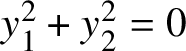 $y_1^2+y_2^2=0$
in
$y_1^2+y_2^2=0$
in
 $\mathbb A^2_{\mathbf {k}}$
is not a Cartesian product as in Theorem 10.2, provided that the field
$\mathbb A^2_{\mathbf {k}}$
is not a Cartesian product as in Theorem 10.2, provided that the field
 $\mathbf {k}$
does not contain a square root of
$\mathbf {k}$
does not contain a square root of
 $-1$
.
$-1$
.
It seems that the triviality techniques from local complex analytic geometry as developed by Ephraim [Reference EphraimEph], extended suitably to the infinite-dimensional context, could be very appropriate to prove such type of results.
We sketch the main ideas: Let
 ${\mathcal Y}={\mathcal Y}(f)\subset \mathcal A_{\circ }^m$
be an arquile variety defined by some power series vector
${\mathcal Y}={\mathcal Y}(f)\subset \mathcal A_{\circ }^m$
be an arquile variety defined by some power series vector
 $f(\mathrm {t},\mathrm {y})\in {\mathcal B}^k$
, and let
$f(\mathrm {t},\mathrm {y})\in {\mathcal B}^k$
, and let
 $y=y(\mathrm {t})\in {\mathcal Y}$
be a point of
$y=y(\mathrm {t})\in {\mathcal Y}$
be a point of
 ${\mathcal Y}$
. We say that
${\mathcal Y}$
. We say that
 ${\mathcal Y}$
is analytically trivial at y if the completed local ring
${\mathcal Y}$
is analytically trivial at y if the completed local ring
 $\widehat {\mathcal O}_{{\mathcal Y},y}$
is isomorphic to the factor ring
$\widehat {\mathcal O}_{{\mathcal Y},y}$
is isomorphic to the factor ring
 $\mathbf {k}[[\mathrm {u}_{\infty }]]/J$
of a formal power series ring
$\mathbf {k}[[\mathrm {u}_{\infty }]]/J$
of a formal power series ring
 $\mathbf {k}[[\mathrm {u}_{\infty }]]=\mathbf {k}[[\mathrm {u}_1,\mathrm {u}_2,\ldots ]]$
in countably many variables
$\mathbf {k}[[\mathrm {u}_{\infty }]]=\mathbf {k}[[\mathrm {u}_1,\mathrm {u}_2,\ldots ]]$
in countably many variables
 $\mathrm {u}_j$
by an ideal J which can be generated by series not depending on the first variable
$\mathrm {u}_j$
by an ideal J which can be generated by series not depending on the first variable
 $\mathrm {u}_1$
. This means that the formal neighbourhood of y in
$\mathrm {u}_1$
. This means that the formal neighbourhood of y in
 ${\mathcal Y}$
is isomorphic to a Cartesian product of the formal neighbourhood of
${\mathcal Y}$
is isomorphic to a Cartesian product of the formal neighbourhood of
 $\mathbb A^1_{\mathbf {k}}$
at
$\mathbb A^1_{\mathbf {k}}$
at
 $0$
with the formal neighbourhood of some other arquile variety at a certain point.
$0$
with the formal neighbourhood of some other arquile variety at a certain point.
To simplify the notation, we assume that
 $y=0\in \mathcal A_{\circ }^m$
is the zero-vector, so all coefficients
$y=0\in \mathcal A_{\circ }^m$
is the zero-vector, so all coefficients
 $y_{ij}$
are zero for all i and j. Writing
$y_{ij}$
are zero for all i and j. Writing
 $\widehat {\mathcal O}_{{\mathcal Y},y}$
as a factor ring
$\widehat {\mathcal O}_{{\mathcal Y},y}$
as a factor ring
 $\mathbf {k}[[\mathrm {y}_{m,\infty }]]/I_{\infty }$
for some ideal
$\mathbf {k}[[\mathrm {y}_{m,\infty }]]/I_{\infty }$
for some ideal
 $I_{\infty }$
of
$I_{\infty }$
of
 $\widehat {\mathcal O}_{\mathcal A_{\circ }^m,y}=\mathbf {k}[[\mathrm {y}_{m,\infty }]]=\mathbf {k}[[\mathrm {y}_{ij},\, 1\leq i\leq m,\, j\geq 1]]$
, it is equivalent to say that there exist formal power series
$\widehat {\mathcal O}_{\mathcal A_{\circ }^m,y}=\mathbf {k}[[\mathrm {y}_{m,\infty }]]=\mathbf {k}[[\mathrm {y}_{ij},\, 1\leq i\leq m,\, j\geq 1]]$
, it is equivalent to say that there exist formal power series
 $\varphi _{ij}(\mathrm {y}_{m,\infty })\in \mathbf {k}[[\mathrm {y}_{m,\infty }]]$
, for
$\varphi _{ij}(\mathrm {y}_{m,\infty })\in \mathbf {k}[[\mathrm {y}_{m,\infty }]]$
, for
 $1\leq i\leq m,\, j\geq 1$
, defining a local
$1\leq i\leq m,\, j\geq 1$
, defining a local
 $\mathbf {k}$
-algebra isomorphism
$\mathbf {k}$
-algebra isomorphism
 $\varphi $
of
$\varphi $
of
 $\mathbf {k}[[\mathrm {y}_{m,\infty }]]$
and such that suitable generators of
$\mathbf {k}[[\mathrm {y}_{m,\infty }]]$
and such that suitable generators of
 $\varphi (I_{\infty })$
do not depend on one of the variables
$\varphi (I_{\infty })$
do not depend on one of the variables
 $\mathrm {y}_{ij}$
, say, without loss of generality,
$\mathrm {y}_{ij}$
, say, without loss of generality,
 $\mathrm {y}_{11}$
.
$\mathrm {y}_{11}$
.
If an arquile variety satisfies the assertion of the Grinberg–Kazhdan–Drinfeld theorem at a point y, then it is in particular analytically trivial at that point.
Assume now that
 $I_{\infty }$
is generated by power series
$I_{\infty }$
is generated by power series
 $F_{\ell }\in \mathbf {k}[[\mathrm {y}_{m,\infty }]]$
,
$F_{\ell }\in \mathbf {k}[[\mathrm {y}_{m,\infty }]]$
,
 $\ell \in {\mathbb N}$
, such that the series
$\ell \in {\mathbb N}$
, such that the series
 $\varphi (F_{\ell })$
generate the ideal
$\varphi (F_{\ell })$
generate the ideal
 $\varphi (I_{\infty })$
.Footnote
29
Let
$\varphi (I_{\infty })$
.Footnote
29
Let
 $G_n$
,
$G_n$
,
 $n\in {\mathbb N}$
, be generators of
$n\in {\mathbb N}$
, be generators of
 $\varphi (I)$
not depending on
$\varphi (I)$
not depending on
 $\mathrm {y}_{11}$
. We may then write
$\mathrm {y}_{11}$
. We may then write
 $G_n=\sum _{\ell \in {\mathbb N}}\, a_{n\ell }\cdot \varphi (F_{\ell })$
for suitable power series
$G_n=\sum _{\ell \in {\mathbb N}}\, a_{n\ell }\cdot \varphi (F_{\ell })$
for suitable power series
 $a_{n\ell }\in \mathbf {k}[[\mathrm {y}_{m,\infty }]]$
. This system of equations can be formally derived with respect to
$a_{n\ell }\in \mathbf {k}[[\mathrm {y}_{m,\infty }]]$
. This system of equations can be formally derived with respect to
 $\mathrm {y}_{11}$
and produces as in the finite-dimensional case a regular derivation
$\mathrm {y}_{11}$
and produces as in the finite-dimensional case a regular derivation
 $\Delta $
of
$\Delta $
of
 $\mathbf {k}[[\mathrm {y}_{m,\infty }]]$
which sends all
$\mathbf {k}[[\mathrm {y}_{m,\infty }]]$
which sends all
 $F_{\ell }$
to
$F_{\ell }$
to
 $I_{\infty }$
; cf. [Reference EphraimEph]. So the existence of such a derivation is a necessary criterion for the analytic triviality (it should also be sufficient, but this is not used here).
$I_{\infty }$
; cf. [Reference EphraimEph]. So the existence of such a derivation is a necessary criterion for the analytic triviality (it should also be sufficient, but this is not used here).
Let us carry out this in the example of the arc space of a variety
 $X\subset \mathbb A^m_{\mathbf {k}}$
defined by a Brieskorn polynomial
$X\subset \mathbb A^m_{\mathbf {k}}$
defined by a Brieskorn polynomial
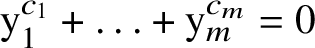 $\mathrm {y}_1^{c_1}+\ldots + \mathrm {y}_m^{c_m}=0$
over a field of characteristic
$\mathrm {y}_1^{c_1}+\ldots + \mathrm {y}_m^{c_m}=0$
over a field of characteristic
 $0$
, with exponents
$0$
, with exponents
 $c_i\geq 2$
. We consider
$c_i\geq 2$
. We consider
 $X_{\infty ,0}$
at the constant arc
$X_{\infty ,0}$
at the constant arc
 $y(\mathrm {t})=0\in \mathbb A^m_{\mathbf {k}}$
. To simplify the notation, we consider only the case
$y(\mathrm {t})=0\in \mathbb A^m_{\mathbf {k}}$
. To simplify the notation, we consider only the case
 $m=2$
and write
$m=2$
and write
 $\mathrm {y}$
for
$\mathrm {y}$
for
 $\mathrm {y}_1$
and
$\mathrm {y}_1$
and
 $\mathrm {z}$
for
$\mathrm {z}$
for
 $\mathrm {y}_2$
, as well as
$\mathrm {y}_2$
, as well as
 $c=c_1$
,
$c=c_1$
,
 $d=c_2$
. The general case
$d=c_2$
. The general case
 $m\geq 2$
goes analogously. From the equation
$m\geq 2$
goes analogously. From the equation
 $\mathrm {y}^c+\mathrm {z}^d=0$
we get the polynomials
$\mathrm {y}^c+\mathrm {z}^d=0$
we get the polynomials
 $$ \begin{align*} \displaystyle F_{\ell}( \mathrm{y}_{\infty}, \mathrm{z}_{\infty})=\sum_{\alpha\in{\mathbb N}^{\mathbb N}, \vert\alpha\vert=c,\vert\vert\alpha\vert\vert=\ell}\, {\mathrm{y}}^{\alpha}_{\infty}+\sum_{\alpha\in{\mathbb N}^{\mathbb N}, \vert\alpha\vert=d,\vert\vert\alpha\vert\vert=\ell}\,{\mathrm{z}}_{\infty}^{\alpha}, \end{align*} $$
where
 $\alpha =(\alpha _1,\alpha _2,\ldots )$
is a string in
$\alpha =(\alpha _1,\alpha _2,\ldots )$
is a string in
 ${\mathbb N}^{\mathbb N}$
with only finitely many nonzero entries,
${\mathbb N}^{\mathbb N}$
with only finitely many nonzero entries,
 $\mathrm {y}^{\alpha }_{\infty }$
stands for the monomial
$\mathrm {y}^{\alpha }_{\infty }$
stands for the monomial
 $\prod _i \mathrm {y}_i^{\alpha _i}$
and where
$\prod _i \mathrm {y}_i^{\alpha _i}$
and where
 $\vert \alpha \vert =\sum _i\alpha _i$
and
$\vert \alpha \vert =\sum _i\alpha _i$
and
 $\vert \vert \alpha \vert \vert =\sum _i i\cdot \alpha _i$
denote the total and weighted degrees of
$\vert \vert \alpha \vert \vert =\sum _i i\cdot \alpha _i$
denote the total and weighted degrees of
 $\mathrm {y}^{\alpha }$
. Denoting by
$\mathrm {y}^{\alpha }$
. Denoting by
 $e_i=(0,\ldots ,0,1,0,\ldots {.})\in {\mathbb N}^{\mathbb N}$
the ith basis vector, we get for all
$e_i=(0,\ldots ,0,1,0,\ldots {.})\in {\mathbb N}^{\mathbb N}$
the ith basis vector, we get for all
 $i\geq 1$
 $$ \begin{align*} \displaystyle {\partial}_{{\mathrm{y}}_i}F_{\ell}(\mathrm{y}_{\infty},\mathrm{z}_{\infty})=\sum_{\alpha\in{\mathbb N}^{\mathbb N}, \vert\alpha\vert=c,\vert\vert\alpha\vert\vert=\ell}\, \alpha_i\cdot {\mathrm{y}}^{\alpha-e_i}_{\infty}. \end{align*} $$
Now observe that for
 $\ell $
fixed, the monomials
$\ell $
fixed, the monomials
 $\mathrm {y}^{\alpha -e_i}$
appearing in the sums are all different for varying
$\mathrm {y}^{\alpha -e_i}$
appearing in the sums are all different for varying
 $\alpha $
and i. Indeed,
$\alpha $
and i. Indeed,
 $\alpha -e_i=\beta -e_j$
implies
$\alpha -e_i=\beta -e_j$
implies
 $\vert \vert \alpha \vert \vert =\vert \vert \beta \vert \vert +i-j=\ell =\vert \vert \beta \vert \vert $
, which is only possible if
$\vert \vert \alpha \vert \vert =\vert \vert \beta \vert \vert +i-j=\ell =\vert \vert \beta \vert \vert $
, which is only possible if
 $i=j$
; this in turn implies that
$i=j$
; this in turn implies that
 $\alpha =\beta $
. But the monomials in
$\alpha =\beta $
. But the monomials in
 $\mathbf {k}[\mathrm {y}_1,\mathrm {y}_2,\ldots ]$
are clearly
$\mathbf {k}[\mathrm {y}_1,\mathrm {y}_2,\ldots ]$
are clearly
 $\mathbf {k}$
-linearly independent, and hence the same holds for the collection of partial derivatives
$\mathbf {k}$
-linearly independent, and hence the same holds for the collection of partial derivatives
 ${\partial }_{\mathrm {y}_i}F_{\ell }$
of
${\partial }_{\mathrm {y}_i}F_{\ell }$
of
 $F_{\ell }$
, for each fixed
$F_{\ell }$
, for each fixed
 $\ell $
(this uses characteristic
$\ell $
(this uses characteristic
 $0$
). Comparing degrees, we conclude that no (finite or infinite)
$0$
). Comparing degrees, we conclude that no (finite or infinite)
 $\mathbf {k}$
-linear combination of the derivatives
$\mathbf {k}$
-linear combination of the derivatives
 ${\partial }_{\mathrm {y}_i}F_{\ell }$
belongs to
${\partial }_{\mathrm {y}_i}F_{\ell }$
belongs to
 $I_{\infty }$
. The same argument applies to the derivative with respect to the variables
$I_{\infty }$
. The same argument applies to the derivative with respect to the variables
 $\mathrm {z}_i$
. Comparing again degrees, one sees that there is actually no regular derivation
$\mathrm {z}_i$
. Comparing again degrees, one sees that there is actually no regular derivation
 $\Delta $
of
$\Delta $
of
 $\mathbf {k}[[\mathrm {y}_{\infty },\mathrm {z}_{\infty }]]$
sending all
$\mathbf {k}[[\mathrm {y}_{\infty },\mathrm {z}_{\infty }]]$
sending all
 $F_{\ell }$
into
$F_{\ell }$
into
 $I_{\infty }$
. By the prospective triviality criterion from above we should then be able to conclude that the formal neighbourhood
$I_{\infty }$
. By the prospective triviality criterion from above we should then be able to conclude that the formal neighbourhood
 $\widetilde X_{\infty ,0}$
of
$\widetilde X_{\infty ,0}$
of
 $X_{\infty ,0}$
at
$X_{\infty ,0}$
at
 $0$
is not analytically trivial. In this case it cannot admit a factorisation as in [Reference Grinberg and KazhdanGK, Reference DrinfeldDr].
$0$
is not analytically trivial. In this case it cannot admit a factorisation as in [Reference Grinberg and KazhdanGK, Reference DrinfeldDr].
Table of symbols
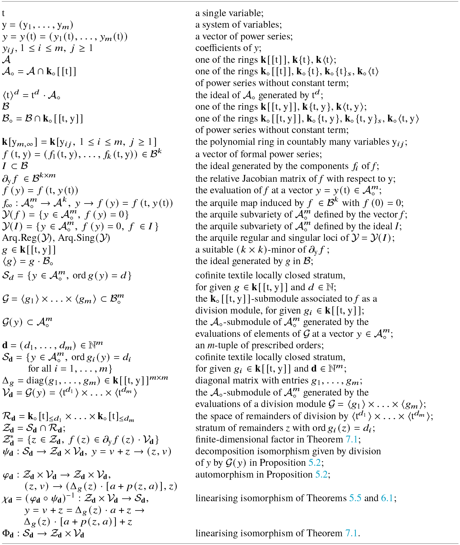
Acknowledgments
The initial phase of the work on this article was carried out in a cooperation of the authors with G. Rond. Numerous discussions with C. Chiu helped to clarify various ambiguities. We are also indebted to D. Popescu, B. Lamel, S. Perlega, H. Kawanoue, F. Castro-Jímenez, M.E. Alonso, M. Spivakovsky and K. Slavov for many helpful conversations and suggestions.
Special thanks go to the anonymous referee: It is seldom to obtain such a competent and detailed report as was the case here. The referee understood the various facets of the article in depth; her/his comments and suggestions were thoughtful and invaluable.
Part of the work was done during the special semester on Artin approximation at CIRM in spring 2015 within the Chaire Jean Morlet of the first-named author at Aix-Marseille University. The hospitality of the personnel at CIRM was greatly appreciated.
Conflict of Interest
None.


 Open access