


Impact Statement
The accurate prediction of laminar/turbulent transition on aircraft wings is of major importance for the design of future low-consumption aircraft. Low atmospheric turbulence rates favour transition triggered by unavoidable surface imperfections. Accurate and straightforward prediction of the flow response to a given wall roughness would pave the way to future shape optimisation or control strategies to efficiently delay transition. However, a general method that accounts for all possible instability mechanisms without any approximation (curvature and non-parallelism) is still lacking. This paper describes a new way to determine the properties of the most critical roughness and its associated response, and to calculate the perturbation amplitude triggered by any given low-amplitude wall roughness.
1. Introduction
The laminar or turbulent nature of the boundary layer has a strong impact on aerodynamic aircraft performance. Thus, predicting laminar–turbulent transition and understanding the transitional mechanisms are crucial. The first stage of the laminar–turbulent transition process is receptivity, by which free-stream fluctuations or surface irregularities are transformed into hydrodynamic instabilities within the boundary layer. These perturbations then grow in the streamwise direction, taking advantage of the local instability mechanisms. In the case of swept wings for example, the three main types of instabilities are attachment line (AL), cross-flow (CF) and Tollmien–Schlichting (TS) instabilities (Reference Reed and SaricReed & Saric 1989). Once sufficiently high perturbation amplitudes are reached, nonlinear effects appear. They trigger saturation or new (secondary) instabilities (Reference HerbertHerbert 1988) which may finally lead to transition. When the free-stream perturbations or the surface irregularities are of small amplitude, a linear theory can be used to describe both the initial receptivity process and the first growth phase.
Reference Deyhle and BippesDeyhle & Bippes (1996) have experimentally shown that transverse travelling CF waves are dominant in boundary layers subjected to a high external turbulence rate ( $Tu>0.2\,\%$), while steady CF waves initiated by surface irregularities dominate for lower turbulence rates, as observed in flight conditions (Reference Carpenter, Saric and ReedCarpenter, Saric & Reed 2008) ( $Tu=0.05\,\%$). Reference Müller and BippesMüller & Bippes (1989) have shown, in the case of a swept flat plate, that steady vortices were triggered by surface irregularities, such as wall roughness. Numerous studies on the receptivity to surface roughness have been carried out during the last decades. Reference Radeztsky, Reibert and SaricRadeztsky, Reibert & Saric (1999) studied experimentally the influence of wall roughness in the case of a swept wing where the initial stability characteristics are CF dominated. They noticed that transition was triggered most upstream when the roughness was located near the AL. Other experimental studies have been conducted and a review of these works on the influence of surface roughness can be found in Reference Saric, Reed and WhiteSaric, Reed & White (2003). From a numerical point of view, Reference CrouchCrouch (1993) studied, in a Falkner–Skan–Cooke (FSC) boundary layer within the parallel-flow assumption, the competition between receptivity triggered by localised perturbations of the surface geometry and by acoustic waves in the free stream. He confirmed that, at high sweep angle, when considering acoustic waves representative of flight conditions, the boundary layer was dominated by the development of steady CFs. Reference Collis and LeleCollis & Lele (1999) dealt with the receptivity to spanwise-periodic surface roughness on a swept parabolic cylinder. They showed that surface curvature and, more significantly, non-parallelism plays an important role in receptivity computations. Reference Schrader, Brandt and HenningsonSchrader, Brandt & Henningson (2009) considered non-parallelism for the study of the receptivity to wall roughness of a three-dimensional boundary layer. They modelled a swept wing leading edge with an FSC-like boundary layer with a favourable pressure gradient. They confirmed that, when the turbulence rate was low, steady CF waves dominated the receptivity process over unsteady CF waves induced by free-stream disturbances. They observed that the receptivity mechanism was fully linear when the height of the roughness was below $5\,\%$ of the displacement thickness. Comparing the results obtained with a meshed roughness in a direct numerical simulation (DNS) and the ones from a parabolised stability equation (PSE) approach with a linear roughness model, Reference Tempelmann, Schrader, Hanifi, Brandt and HenningsonTempelmann et al. (2012b) concluded that the linear model was valid up to a roughness height of $0.1$ of the displacement thickness.
In boundary-layer flow, streamwise energy amplification may also occur due to non-modal (local) effects (even when flows are exponentially spatially stable). Contrary to two-dimensional boundary layers, few studies exist on the non-modal growth of three-dimensional boundary layers. Reference Corbett and BottaroCorbett & Bottaro (2001) have computed, in the case of the FSC within parallel-flow assumption, the perturbations with the largest transient gain over a fixed period of time. They showed that, in contrast to the two-dimensional case, both modal and non-modal growths exhibit similar structures, with the optimal perturbations evolving into vortices almost aligned with the direction of the outer flow, which finally trigger streaks with the lift-up mechanism. These observations were confirmed by Reference Tempelmann, Hanifi and HenningsonTempelmann, Hanifi & Henningson (2010), who studied the same flow using a spatial framework and PSEs, allowing them to take into account non-parallel effects.
In order to capture all instability mechanisms (AL, CF, TS, non-modal) and the effects of non-parallelism and surface curvature, global stability analyses (at least in the chordwise direction) on a swept profile were initiated by Reference Tempelmann, Hanifi and HenningsonTempelmann, Hanifi & Henningson (2012a). They used solutions of the adjoint linearised Navier–Stokes (ALNS) equations to explore the receptivity of CF perturbations on a swept wing of infinite span. They studied in particular the roughness shape leading to the perturbations with the largest amplitude at the domain outflow. It corresponds to a wavy shape in the chordwise direction that is maximal in the vicinity and just downstream of the AL. The method relies on global direct (respectively adjoint) stability computations with an upstream (respectively downstream) Dirichlet boundary condition determined with a local spatial direct (respectively adjoint) stability computation. The computational domain therefore needs to be chosen in such a way that the same local instability branch be identified at the upstream (direct) and downstream (adjoint) boundaries, which requires some tuning and a precise knowledge of the instability mechanisms. Reference Thomas, Mughal and AshworthThomas, Mughal & Ashworth (2017) used a similar method and a large number of receptivity calculations have been performed for different forcing by computing only once the solutions of the linearised Navier–Stokes (LNS) and ALNS equations. In particular, they have confirmed that CF instabilities were more affected by roughness near the AL.
The present paper aims at studying the receptivity to small-amplitude wall roughness by considering a dedicated transfer function, whose input is a small-amplitude wall deformation (instead of the volume forcing in resolvent analysis Reference Trefethen, Trefethen, Reddy and DriscollTrefethen et al. 1993; Reference Schmid and HenningsonSchmid & Henningson 2001), while the output remains, as in resolvent analysis, the full-state perturbation. The modelling of the wall deformation is based on a linear model, the validity of which has been examined notably by Reference Schrader, Brandt and HenningsonSchrader et al. (2009) and Reference Tempelmann, Schrader, Hanifi, Brandt and HenningsonTempelmann et al. (2012b). The singular value decomposition of resolvent operators has been widely used to study the energy amplification due to both modal and non-modal mechanisms in transitional flows (Reference Sipp and MarquetSipp & Marquet 2013; Reference Symon, Rosenberg, Dawson and McKeonSymon et al. 2018). It allows us to consider the non-modal mechanisms and to take into account non-parallelism in boundary layer or free-shear flows. Compared with the method used by Reference Thomas, Mughal and AshworthThomas et al. (2017) and Reference Tempelmann, Hanifi and HenningsonTempelmann et al. (2012a), it also has the benefit of not relying on relevant inlet/outlet boundary conditions, that come from local direct and adjoint spatial stability solutions: such a method in particular requires us to identify a local spatial mode at the inlet of the computational domain that is connected to a local spatial mode at the outlet of the domain. Hence, only local modal spatial instabilities can be dealt with when using that method and the inlet and outlet boundaries need to be located in specific regions (for the case considered in the present article, we will even show that it is not possible to follow this mode from the inlet to the outlet of the domain). Note that a PSE-based method instead of local spatial stability analysis could mitigate this problem: yet, this method still needs to be initialised at the inlet by a local spatial mode and it does not handle local non-modal instabilities (Reference Towne, Rigas and ColoniusTowne, Rigas & Colonius 2019). In contrast, the present transfer function-based method does not suffer from these limitations since it is the optimisation process of the input–output dynamics that automatically identifies the most energetic forcings and responses, even in the case of local non-modal instabilities and in the case of strong non-parallelism. Also, considering the transfer function associated with the full LNS equations gives access to the response amplitude in the vicinity of the location of the roughness and the use of the singular value decomposition has the advantage of providing two orthonormal bases, one for the input space and one for the output space. When a singular value is strongly dominant, the analysis gives intrinsic information about the physics of the flow by showing the leading instability mechanism, both in response and in forcing. In this case, once a few optimal forcings and responses have been computed, the calculation of the response to a given roughness can be approximated by only computing a few scalar products. Moreover, the prediction of the full response based on the dominant optimal forcings/responses will be accurate downstream of the roughness, which is usually sufficient for laminar/turbulent transition predictions. We will assess the accuracy of the prediction when using the dominant singular value for both periodic and compact roughness in the chordwise and spanwise directions. The method will be illustrated on the swept ONERA-D aerofoil, a configuration that was already studied (base-flow and neutral stability curves of AL, CF and TS perturbations) in Reference Kitzinger, Leclercq, Marquet, Piot and SippKitzinger et al. (2023).
The outline of the paper is the following. In § 2, we describe the flow configuration, in § 3 the wall displacement-based transfer function and the approximations and in § 4 the numerical methods. In § 5, the results are illustrated for the ONERA-D aerofoil. The properties of the optimal roughness and responses are explored in § 5.1 and the perturbations triggered by particular roughness are studied in § 5.2. We validate, in particular, in this last sub-section the low-rank approximation against the exact response (given by the transfer function) for various roughness shapes.
2. Flow configuration
We investigate the incompressible flow around an aerofoil of chord  $C$ and of infinite span. The origin of the orthonormal coordinate system $(x,y,z)$ is located at the leading edge of the aerofoil, whose direction is denoted $z$. As shown in figure 1, the $x$- and $y$-directions are orthogonal to the leading edge and to the symmetry plane of the aerofoil, respectively. The uniform upstream velocity is of constant magnitude $U^{\infty }$ and oriented in a direction defined by the sweep angle $\varLambda$ and the angle of attack $\alpha$, that is zero in the present study. The sweep velocity denoted $U_z^\infty =U^\infty \sin \varLambda$ is the component of the upstream velocity in the spanwise direction while the chordwise velocity $U_x^\infty =U^\infty \cos \varLambda$ is the component in the chordwise direction. Note that $C$ denotes the aerofoil's chord in the direction of the upstream velocity while $C_n= C \cos \varLambda$ is the chord normal to the aerofoil's leading edge. In the following, all variables are made non-dimensional using the chord $C_n$ and the velocity $U_x^\infty$. The incompressible flow is entirely characterised by two non-dimensional parameters: the sweep angle $\varLambda$ and the Reynolds number $Re_{C_n}=U_x^\infty C_n / \nu$, $\nu$ being the kinematic viscosity of the fluid. The local coordinate system $(s,\eta,z)$ is shown in the close-up view of figure 1(a). Here, $s$ is the curvilinear abscissa along the surface of the profile in the plane orthogonal to the spanwise $z$-direction and $\eta$ the local wall normal direction. Thus, $\eta =0$ corresponds to the aerofoil's wall. The local direction of the streamline of the external base-flow velocity field $\chi$ is shown in figure 1(b).
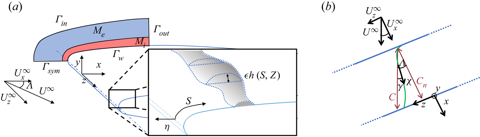
Figure 1. (a) Schematic of the mesh and flow configuration with a zoom on a roughness of any shape. (b) Angles and coordinate systems are indicated. An external streamline is illustrated in green. The blue lines correspond to the leading/trailing edges.
3. Theory
We investigate the incompressible three-dimensional steady flow surrounding a rough aerofoil infinitely long in the spanwise direction  $z$. The non-dimensional flow velocity $\boldsymbol {U}_{T}(x,y,z)$ and pressure $P_{T}(x,y,z)$ fields are governed by the steady incompressible Navier–Stokes equations
 \begin{equation} ( \boldsymbol{U}_{T} \boldsymbol{\cdot} \boldsymbol{\nabla} ) \boldsymbol{U}_{T} + \boldsymbol{\nabla} P_{T} - Re_{C_{n}}^{{-}1}{\nabla}^2 \boldsymbol{U}_{T} = \boldsymbol{0}, \quad \boldsymbol{\nabla} \boldsymbol{\cdot} \boldsymbol{U}_{T} = 0 \mbox{ in } \varOmega_{r}, \quad \boldsymbol{U}_{T} = \boldsymbol{0} \mbox{ on } \varGamma_{r}, \end{equation}
where the gradient is classically defined as  $\boldsymbol {\nabla }=(\partial _x,\partial _y,\partial _z)^T$. The momentum and mass equations are satisfied in the spatial domain $\varOmega _{r}$ surrounding the aerofoil and the roughness. The boundary formed by the aerofoil and the roughness is denoted $\varGamma _r$, on which a no-slip velocity condition is imposed.
As sketched in the close-up view of figure 1(a), we further assume that the height of any wall roughness, denoted  $\epsilon h(s,z)$, is infinitesimally small compared with the thickness/chord of the smooth aerofoil, the surface of the latter being denoted $\varGamma _w$. In the local curvilinear coordinate system, the surface of $\varGamma _r$ is thus described by $(s,\eta =\epsilon h(s,z), z)$, with $\epsilon \ll 1$, while the surface of the smooth aerofoil $\varGamma _w$ is $(s,\eta =0, z)$. The roughness being considered as a small perturbation of the smooth aerofoil geometry, we decompose the flow variables as
 \begin{equation} (\boldsymbol{U}_{T},P_{T}) = (\boldsymbol{U},P) + \epsilon (\boldsymbol{u},p), \end{equation}
where  $(\boldsymbol {U},P)$ denotes the flow over the smooth aerofoil while $(\boldsymbol {u},p)$ is the flow perturbation induced by the roughness. This decomposition is injected into the governing equations (3.1) to obtain, at zeroth order, the equations the flow around the smooth aerofoil, and at $\epsilon$ order the wall roughness perturbation equations. In particular, the no-slip boundary condition along $\varGamma _r$ reads
 \begin{equation} \boldsymbol{0} = \boldsymbol{U}_{T}(s,\epsilon h(s,z),z) \approx \boldsymbol{U}(s,0,z) + \epsilon [ \boldsymbol{u} + h \partial_\eta \boldsymbol{U} ](s,0,z) + \cdots. \end{equation}
This Taylor expansion shows that, at first order in  $\epsilon$, the small roughness is equivalent to the velocity perturbation over the smooth aerofoil
 \begin{equation} \boldsymbol{u}(s,0,z) = {-} h \partial_\eta \boldsymbol{U}. \end{equation}
The validity of this linearised velocity condition for modelling the effect of a roughness on a boundary-layer flow was addressed by Reference Schrader, Brandt and HenningsonSchrader et al. (2009) and Reference Tempelmann, Schrader, Hanifi, Brandt and HenningsonTempelmann et al. (2012b), who found that this is a valid approximation for a roughness height below  $0.05\delta ^*$, $\delta ^*$ being the displacement thickness of the boundary layer.
3.1 Steady flow over the smooth aerofoil
The equations governing the base-flow velocity field  $\boldsymbol {U}(x,y)=(U,V,W)^{T}$ around the swept smooth aerofoil are the steady Navier–Stokes equations
 \begin{equation} ( \boldsymbol{U} \boldsymbol{\cdot} \boldsymbol{\nabla} ) \boldsymbol{U} + \boldsymbol{\nabla} P - Re_{C_{n}}^{{-}1} {\nabla}^2 \boldsymbol{U} = \boldsymbol{0}, \quad \boldsymbol{\nabla} \boldsymbol{\cdot} \boldsymbol{U} = \boldsymbol{0} \mbox{ in } \varOmega, \quad \boldsymbol{U} = \boldsymbol{0} \mbox{ on } \varGamma_w. \end{equation}
As the aerofoil is symmetric and the angle of attack is zero, the domain  $\varOmega$ may be restricted to the upper half-domain, i.e. $y>0$. A symmetric boundary condition $(\partial _y U_x, U_y, \partial _y U_z)=(0,0,0)$ is applied at the symmetric boundary $\varGamma _{sym}=\{x<0,y=0\}$. As shown in figure 1(a), the spatial domain $\varOmega$ does not extend up to the trailing edge of the aerofoil. To specify the boundary conditions at the inflow $\varGamma _{in}$ and outflow $\varGamma _{out}$ boundaries of this domain, we first determine the symmetric potential velocity field $(U_x^p,U_y^p,U_z^p)=(\partial _y \psi, -\partial _x \psi,U_z^\infty =\tan (\varLambda ))$ with the streamfunction $\psi$ satisfying the Laplace equation ${\rm \Delta} \psi = 0$, in a sufficiently large domain $\varOmega _{p}$ so that we may impose the uniform velocity condition $\psi = y$ on the far-field boundary $\varGamma _p$. On $\varGamma _w$ and $\varGamma _{sym}$, we set $\psi =0$, which allows the smooth aerofoil to be a streamline and the flow field to be symmetric. This potential velocity is then imposed as a Dirichlet boundary condition at the inlet boundary $\varGamma _{in}$ of the domain $\varOmega$, i.e.
 \begin{equation} (U_x,U_y,U_z) = (U_x^{p},U_y^{p},U_z^\infty) \textrm{ on } \varGamma_{in}, \end{equation}
while the pressure field of the potential flow  $P^p=[1-(U_x^{p})^2-(U_y^{p})^2]/2$ and a Neumann condition for the velocity field are applied at the outlet
 \begin{equation} \partial_x \textbf{U} = \textbf{0} \quad \mbox{and} \quad P = P^{p} \mbox{ on } \varGamma_{out}. \end{equation}
3.2 Wall displacement induced perturbation
We consider a roughness that may be harmonic, periodic or compact in either the curvilinear  $s$- or spanwise $z$-directions. The linear equations governing the three-dimensional flow perturbation $(\boldsymbol {u},p)(x,y,z)$ induced by this roughness are
 \begin{equation} ( \boldsymbol{u} \boldsymbol{\cdot} \boldsymbol{\nabla} ) \boldsymbol{U} + ( \boldsymbol{U} \boldsymbol{\cdot} \boldsymbol{\nabla} ) \boldsymbol{u} + \boldsymbol{\nabla} p - {Re_{C_{n}}^{{-}1}} {\nabla}^2 \boldsymbol{u} = \boldsymbol{0}, \quad \boldsymbol{\nabla} \boldsymbol{\cdot} \boldsymbol{u} = 0 \mbox{ in } \varOmega \quad \boldsymbol{u} = {-} h \partial_\eta \boldsymbol{U} \mbox{ on } \varGamma_w. \end{equation}
As explained before, the presence of the roughness over the smooth aerofoil is accounted for with the linearised wall boundary condition. The solution of the above linear problem with non-homogeneous boundary conditions at the wall is the sum of the solution of the problem with a homogeneous condition and a particular forced solution. We choose the Reynolds number and sweep angle so as to have a globally stable base flow, so that all homogeneous solutions tend to zero at large times. We hence only consider the forced response. Interestingly, the spanwise dependency of the flow perturbation is only due to the spanwise dependency of the roughness  $h(s,z)$, since the velocity $\boldsymbol {U}$ is invariant in the spanwise direction. Hence, any roughness and triggered perturbation can be further decomposed into Fourier modes as
 \begin{equation} h(s,z) = \int_{-\infty}^{\infty} \hat{h}_{\beta}(s)\, {\rm e}^{{\rm i} \beta z} \, {\rm d} \beta,\quad \boldsymbol{u}(x,y,z) = \int_{-\infty}^{\infty} \boldsymbol{\hat{u}}_{\beta}(x,y)\, {\rm e}^{{\rm i} \beta z} \, {\rm d}\beta, \end{equation}
where  $\beta$ is the (real) spanwise wavenumber and the corresponding (complex) Fourier modes of the wall roughness and flow response are denoted $\hat {h}_{\beta }(s)$ and $\boldsymbol {\hat {u}}_{\beta }(x,y)$, respectively. Note that the case of periodic roughness in $z$ may be handled by stating that $\hat {h}_\beta (s)=\sum _m \delta (\beta -m\beta _0) \hat {h}_{m\beta _0}(s)$, with $\beta _0=2{\rm \pi} /L_z$ being the fundamental wavenumber in $z$ and $\delta (\beta )$ the Dirac function at $\beta =0$. Since the three-dimensional roughness $h(s,z)$ and flow perturbation $\boldsymbol {u}(x,y,z)$ are real quantities, the corresponding complex Fourier modes satisfy $\hat {h}_{-\beta } = \overline {\hat {h}_{\beta }}$ and $\boldsymbol {\hat {u}}_{-\beta } = \overline {\boldsymbol {\hat {u}}_{\beta }}$, where $\overline {(\cdot )}$ denotes the complex conjugate.
Injecting this Fourier decomposition into (3.8), we obtain
 \begin{align} \left. \begin{array}{c} ( \boldsymbol{\hat{u}}_{\beta} \boldsymbol{\cdot} \boldsymbol{\nabla} ) \boldsymbol{U} + ( \boldsymbol{U} \boldsymbol{\cdot} \boldsymbol{\nabla}_{\beta} ) \boldsymbol{\hat{u}}_{\beta} + \boldsymbol{\nabla}_{\beta} \hat{p}_{\beta} - {Re_{C_{n}}^{{-}1}} \boldsymbol{\nabla}_{\beta}^2 \boldsymbol{\hat{u}}_{\beta} = \boldsymbol{0}, \quad \boldsymbol{\nabla}_{\beta} \boldsymbol{\cdot} \boldsymbol{\hat{u}}_{\beta} = 0 \mbox{ in } \varOmega \Rightarrow \mathcal{L}_\beta\boldsymbol{\cdot}(\boldsymbol{\hat{u}}_{\beta},\hat{p}_{\beta})^T = \boldsymbol{0} \mbox{ in } \varOmega , \\ \boldsymbol{\hat{u}}_{\beta} = {-} \hat{h}_\beta \partial_\eta \boldsymbol{U}\mbox{ on } \varGamma_w \Rightarrow \hat{u}_{\beta} = \mathcal{F}\hat{h}_\beta\mbox{ on } \varGamma_w, \end{array} \right\} \end{align}
where the gradient and Laplacian operators applied to the Fourier modes are defined as  $\boldsymbol {\nabla }_{\beta }=(\partial _x,\partial _y,\rm {i} \beta )^{T}$. Here, $\mathcal {L}_\beta$ is the linearised Navier–Stokes operator and $\mathcal {F}$ is the operator that transforms the wall normal displacement $\hat {\boldsymbol {h}}_{\beta }$ into a velocity $\hat {\boldsymbol {u}}_{\beta }$ with appropriate Dirichlet boundary conditions on the wall and zeros inside the domain. The boundary conditions at the inflow and outflow boundaries are $\boldsymbol {\hat {u}}_{\beta } = \textbf {0}$ on $\varGamma _{in}$ and $\hat {p}_{\beta } \boldsymbol {e}_x-Re_{C_n}^{-1} \partial _x \boldsymbol {\hat {u}}_{\beta } = 0$ on $\varGamma _{out}$ and we restrict our analysis to symmetric perturbations, i.e. $( \partial _y \hat {u}_{\beta,x}, \hat {u}_{\beta,y}, \partial _y \hat {u}_{\beta,z} ) = (0,0,0) \mbox { on } \varGamma _{sym}$. We can thus calculate the flow perturbation triggered by a roughness over the smooth aerofoil without modifying the geometry, by using the steady flow $\boldsymbol {U}$ over the smooth aerofoil and by applying the linearised wall velocity condition at its surface.
After spatial discretisation, the (3.10) with the above boundary conditions can be recast in an input–output form
 \begin{equation} \boldsymbol{\hat{u}}_{\beta} = R_\beta \hat{\boldsymbol{h}}_{\beta}, \end{equation}
where  $R_{\beta }=P^*L_\beta ^{-1}PF$. The matrices $L_\beta$ and $F$ are respectively the discrete forms of the continuous operators $\mathcal {L}_\beta$ and $\mathcal {F}$ defined in (3.10). The matrix $P$ designates the prolongation operator which adds a zero pressure component to a given velocity vector.
The parameter  $\hat {\boldsymbol {h}}_{\beta }$ denotes the discrete vector of the function $\hat {h}_{\beta }(s)$, and $\boldsymbol {\hat {u}}_{\beta }$ is the discrete velocity vector of the continuous vectorial field $\boldsymbol {\hat {u}}_{\beta }(x,y)$. In the following, the spatial coordinates $(x,y)$ are specified to distinguish the continuous and discrete forms of the velocity vector; $R_{\beta }$ designates a transfer function taking a wall roughness Fourier mode $\boldsymbol {\hat {h}}_{\beta }$ as input and giving the flow-perturbation Fourier mode $\boldsymbol {\hat {u}}_{\beta }$ as output.
3.3 Transfer function from wall displacement to induced velocity-perturbation field
We will now determine two orthonormal bases, one for the (input) wall roughness Fourier modes and one for the (output) flow-response Fourier modes. For this, we define the kinetic energy of the triggered perturbation  $\langle \boldsymbol {\hat {u}}_{\beta }(x,y),\hat {\boldsymbol {u}}_{\beta }(x,y)\rangle = \int _\varOmega \boldsymbol {\hat {u}}_{\beta }^*(x,y) \boldsymbol {\hat {u}}_{\beta }(x,y) \, \textrm {d} x\, \textrm {d} y$ in the domain $\varOmega$, which is a measure of the output space, where $(\cdot )^*$ refers to the transconjugate and $\langle {\hat {h}}_{\beta }(s),{\hat {h}}_{\beta }(s)\rangle _{w} = \int _{\varGamma _w} \overline {\hat {h}_{\beta }(s)}\hat {h}_{\beta }(s)\,\textrm {d} s$ is a measure of the input space. The discrete form for each measure is then denoted $\boldsymbol {\hat {u}}_{\beta }^* Q_u \boldsymbol {\hat {u}}_{\beta }$ and $\boldsymbol {\hat {h}}_{\beta }^* Q_h \boldsymbol {\hat {h}}_{\beta }$, respectively. Then, we introduce the energetic gain $G_{\beta }$ to be maximised as the ratio between the output and input measures, i.e.
 \begin{equation} G_{\beta} = \frac{\boldsymbol{\hat{u}}_{\beta}^ * Q_u \boldsymbol{\hat{u}}_{\beta}}{\boldsymbol{\hat{h}}_{\beta}^ * Q_h \boldsymbol{\hat{h}}_{\beta}} = \frac{\boldsymbol{\hat{h}}_{\beta}^ * R_\beta^ * Q_u R_\beta \boldsymbol{\hat{h}}_{\beta}}{\boldsymbol{\hat{h}}_{\beta}^ * Q_h \boldsymbol{\hat{h}}_{\beta}}, \end{equation}
where the input–output relation (3.11) has been used in the numerator. The solution of the optimisation problem  $max_{\boldsymbol {\hat {h}}_{\beta }}G_{\beta }$ and the optimal roughness/responses are finally obtained by solving the two problems
 \begin{equation} R_\beta^ * Q_u R_\beta \boldsymbol{\hat{h}}_{\beta,j} = \sigma_{\beta,j}^2 Q_h \boldsymbol{\hat{h}}_{\beta,j}, \quad \boldsymbol{\hat{u}}_{\beta,j} = \sigma_{\beta,j}^{{-}1} R_\beta \boldsymbol{\hat{h}}_{\beta,j}. \end{equation}
The optimal roughness  $\boldsymbol {\hat {h}}_{\beta,j}$ and optimal flow responses are normalised as $\langle {\hat {h}}_{\beta,j}(s),{\hat {h}}_{\beta,j}(s)\rangle _{w}=1$ and $\langle \boldsymbol {\hat {u}}_{\beta,j}(x,y),\hat {\boldsymbol {u}}_{\beta,j}(x,y)\rangle =1$. Note that a fully continuous framework for the definition of these quantities also exists but is not shown here for conciseness. The set of eigenvectors $({\hat {h}}_{\beta,j}(s))_{j\geq 1}$ form an orthonormal basis of the forcing space with respect to $\langle \cdot,\cdot \rangle _w$, while the optimal responses $(\boldsymbol {\hat {u}}_{\beta,j})(x,y)_{j\geq 1}$ constitute an orthonormal basis of the response space with respect to $\langle \cdot,\cdot \rangle$. In our study, we sort the singular values such that $\sigma _{\beta,1}\geq \sigma _{\beta,2}\geq \sigma _{\beta,3}\geq \cdots$, so that the optimal forcing ${\hat {h}}_{\beta,1}(s)$ is related to $\sigma _{\beta,1}^2=max_{\boldsymbol {\hat {h}}}G_\beta$.
We can now compute the response  $\boldsymbol {\hat {u}}_{\beta }(x,y)$ in (3.11) using the input and output bases
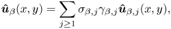 \begin{equation} \boldsymbol{\hat{u}}_{\beta}(x,y) = \sum_{j\geq1} \sigma_{\beta,j} \gamma_{\beta,j} \boldsymbol{\hat{u}}_{\beta,j}(x,y), \end{equation}
with  $\gamma _{\beta,j}=\langle \hat {h}_{\beta,j}(s),\hat {h}_{\beta }(s)\rangle _w$ the projection coefficients of the wall roughness Fourier mode $\hat {h}_{\beta }(s)$ onto the optimal roughness $\hat {h}_{\beta,j}(s)$. In the case where the first singular value is much larger than the following ones, which is generically the case when an instability mechanism is at play, we can neglect the contribution of the next terms: if $\sigma _{\beta,1}\;\lvert \gamma _{\beta,1} \rvert \gg \sigma _{\beta,j} \lvert \gamma _{\beta,j} \rvert \ \forall \, {j\geq 2}$, we can consider only the contribution of the dominant optimal response: $\boldsymbol {\hat {u}}_{\beta }(x,y) \approx \sigma _{\beta,1} \gamma _{\beta,1} \boldsymbol {\hat {u}}_{\beta,1}(x,y)$.
We then obtain an approximation of the response  $\boldsymbol {u}(x,y,z)$ triggered by the roughness $h(s,z)$ following
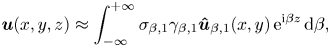 \begin{equation} \boldsymbol{u}(x,y,z) \approx \int_{-\infty}^{ + \infty} \sigma_{\beta,1} \gamma_{\beta,1} \boldsymbol{\hat{u}}_{\beta,1}(x,y)\, {\rm e}^{{\rm i}\beta z}\,{\rm d} \beta, \end{equation}
and the local perturbation energy averaged over the spanwise direction reads
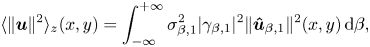 \begin{equation} \langle\|\boldsymbol{u}\|^2\rangle_z(x,y) = \int_{-\infty}^{ + \infty} \sigma_{\beta,1}^2 |\gamma_{\beta,1}|^2 \|\boldsymbol{\hat{u}}_{\beta,1}\|^2(x,y) \, {\rm d} \beta, \end{equation}
where  $\langle \cdot \rangle _z =\lim _{L_z \rightarrow \infty } (1/L_z) \int _0^{L_z} (\cdot ) \,\textrm {d} z$. Explicit approximations may then be obtained by evaluating the integral with a fourth-order extended Simpsons's rule (Reference Press, Teukolsky, Vetterling and FlanneryPress et al. 2007) over a finite wavenumber range, as discussed in § 5.2.2.
4. Numerical methods
All numerical aspects are handled with FreeFEM (Reference HechtHecht 2012), an open-source partial-differential-equation solver that allows us to implement spatial discretisation with the finite element method. Solutions of resulting large-scale linear problems are computed on multiple processors using the FreeFEEM interface with the Portable, Extensible Toolkit for Scientific Computation (PETSc) (Reference BalayBalay et al. 2022). The interface with the scalable library for eigenvalue problem computations (SLEPc) solver (Reference Hernandez, Roman and VidalHernandez, Roman & Vidal 2005) is used to compute the solutions to eigenvalue problems. We refer to Reference Moulin, Jolivet and MarquetMoulin, Jolivet & Marquet (2019) for didactic examples of these two interfaces in the context of the linear stability analysis of large-scale hydrodynamic eigenvalue problems. Taylor–Hood finite elements are used for the spatial discretisation of nonlinear base-flow (3.5) and linear perturbation equations (3.10). The velocity and pressure fields are respectively expanded on second-order ( $P_2$) and first-order ( $P_1$) Lagrange finite elements. A streamline-upwind Petrov–Galerkin (SUPG) method together with grad–div stabilisation (Reference Ahmed and RubinoAhmed & Rubino 2019) is used to compute the base-flow solution while no SUPG stabilisation is considered for the perturbation. A Newton–Raphson method is implemented in FreeFEM to compute solutions of the nonlinear base-flow equations (3.5), using the potential flow solution as initial condition of this iterative algorithm. The direct sparse LU-solver MUMPS (Reference Amestoy, Duff, Koster and L'ExcellentAmestoy et al. 2001, Reference Amestoy, Buttari, L'Excellent and Mary2019) is called within PETSc to compute the solution of linear problems at each iteration of the algorithm. To compute the largest eigenvalues of the eigenproblem (3.13a,b), a Krylov–Schur algorithm is used. The application of the matrices $R_\beta$ and $R_\beta ^*$ to input vectors provided by the Krylov–Schur algorithm requires the solution of linear problems that are obtained with the MUMPS solver, again.
As shown in figure 1, we consider a two-dimensional domain  $\varOmega$ covering the upper half of the aerofoil and which extends up to $15\,\%$ in the chordwise $x$-direction. Two different body-fitted meshes are used to compute the base flow and to solve the eigenproblem (3.13a,b). For the base-flow solution, this mesh is composed of $120\ 000$ triangles. It is made up of an internal $M_i$ part (red in figure 1, $100 000$ triangles) and an external $M_e$ part (blue, $20\ 000$ triangles). To solve the eigenproblem (3.13a,b), we use only the internal mesh $M_i$, the boundary $\varGamma _{in}$ being sufficiently far from the profile so that 0-Dirichlet boundary conditions may be imposed. For more details, we refer the reader to Reference Kitzinger, Leclercq, Marquet, Piot and SippKitzinger et al. (2023), where the same mesh was used to perform global stability analysis of the base-flow solution. In particular, the effect of the chordwise extension of the domain and of grid refinement was assessed for the computation of base flows and neutral curves (marginal eigenvalues of the Jacobian $L_\beta$). A similar convergence study (not reported here) was performed for the singular values and singular modes to insure that reported results are robust to spatial discretisation.
5. Results
In the present study, we consider the parameters  $Re_{C_n}=1.39 \times 10^6$, $\varLambda =65.8^\circ$, which correspond to a globally stable flow for all spanwise wavenumbers (Reference Kitzinger, Leclercq, Marquet, Piot and SippKitzinger et al. 2023) and thus allows the input–output analysis described in § 3.3. In that study, the Reynolds number and sweep angle were chosen to allow the computation of the neutral curve associated with the various instabilities, which remains simple only at high sweep angles. Yet, for the present study, which relies on a more robust transfer function analysis to characterise the instabilities, lower sweep angles could have been chosen. We decided to keep the initial parameters to focus the paper on the novelty, which is methodological. Hence, extensive discussions about the base-flow solution can be found in Reference Kitzinger, Leclercq, Marquet, Piot and SippKitzinger et al. (2023). We recall that it was validated by comparing the external streamline velocity component and the CF component within the boundary layer with those obtained by using an ONERA in-house boundary-layer code which solves the Prandtl equations (Reference HoudevilleHoudeville 1992). We observed a close agreement between the results obtained with both methods.
For the description of the results, the spanwise wavenumber  $\beta$ of the perturbations will be scaled with $\varDelta$, which is a measure of the boundary-layer thickness at the AL based on the potential flow (Reference Mack and SchmidMack & Schmid 2011). It is defined as $\varDelta = \partial U_s^{p}/\partial s|_{x=0,y=0}$, where $U_s^{p}$ denotes the $s$-component of the potential flow solution. In Reference Kitzinger, Leclercq, Marquet, Piot and SippKitzinger et al. (2023), it was shown that this thickness corresponds to the displacement thickness at the AL. For the present configuration, we have $\varDelta =9.71 \times 10^{-5}$.
5.1 Wall displacement input modes
Figure 2 shows the first two singular values  $\sigma _1$ and $\sigma _2$ as a function of the spanwise wavenumber $0 \leq \beta \varDelta \leq 0.5$. For values of $\beta \varDelta$ between $0.05$ and $0.2$, the first singular value is significantly higher than the second one, making the transfer function nearly rank 1. The second singular value has a maximum of $\sigma _2=415$ reached for $\beta \varDelta =0.08$, while the maximum of the first singular value is achieved for $\beta \varDelta =0.11$, where $\sigma _1=12\ 162$. The singular value $\sigma _1$ for $\beta \varDelta =0.11$, highlighted by the black circle, corresponds to the configuration that is studied in more detail in the following.
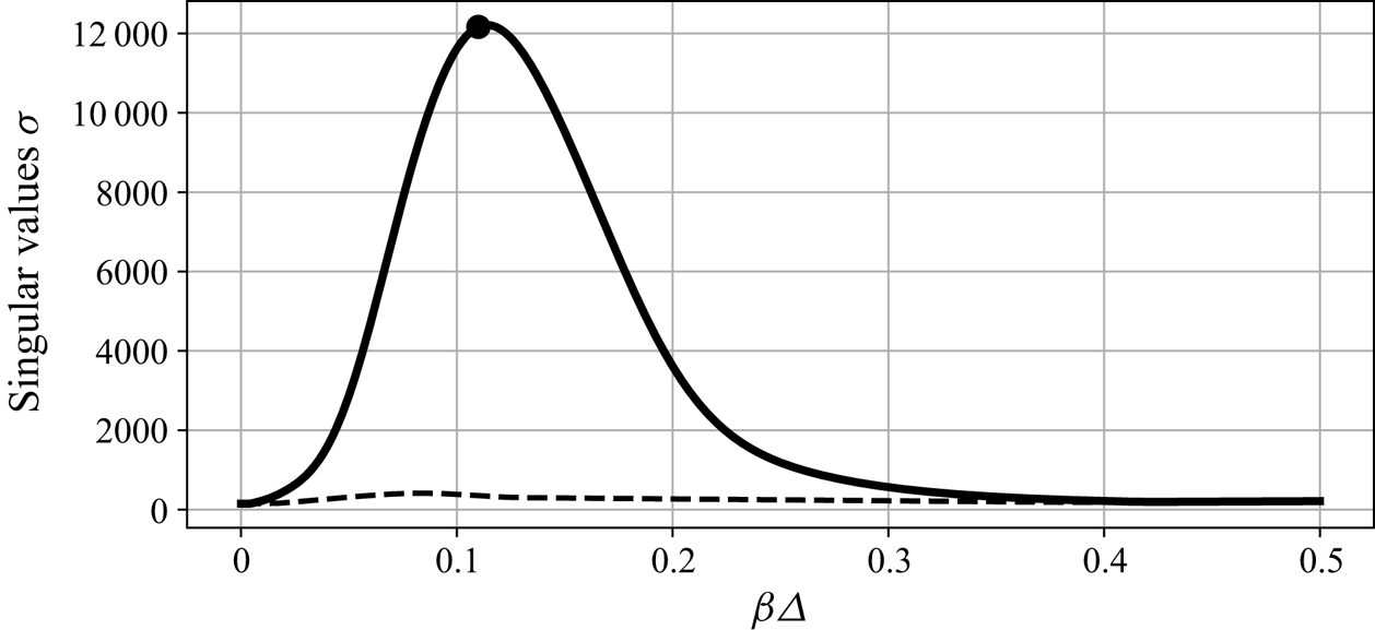
Figure 2. First two singular values:  $\sigma _1$ in solid line and $\sigma _2$ in dashed line. The largest singular value ( $\beta \varDelta =0.11$) is marked with a circle.
5.1.1 Optimal roughness and response for  $\beta \varDelta =0.11$

We now analyse the spatial structure of the optimal response and roughness for a spanwise wavenumber close to the largest singular value, i.e.  $\beta \varDelta =0.11$. In figure 3 we represent the iso-surfaces of the real part of the optimal roughness and of the spanwise velocity of the optimal response. The optimal roughness is located at the beginning of the leading edge and is oriented in a direction close to the external streamline. The optimal response has a large magnitude on the whole leading edge, except at the AL. It consists in steady vortices whose axes are nearly parallel to the external streamlines.
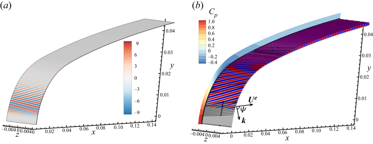
Figure 3. Spatial structure of the real part of: the optimal roughness  $\Re (\hat {h}_{0.11/\varDelta,1}(s)\, \textrm {e}^{\textrm {i}\beta z})$ (a) and the $z$-velocity of the response $\Re (\hat {u}_{0.11/\varDelta,1,z}(x,y)\, \textrm {e}^{\textrm {i}\beta z})$ (b). Two iso-surfaces at $\pm 0.1$ times the absolute maximum are represented in red and blue. Pressure coefficient $C_p$, boundary-layer thickness $\delta _{99}$ (black line) and potential streamlines (black arrow lines) are shown. An example of the wavevector and $\varPsi$ angle is also displayed.
To help discern the type of instability, as commonly done in local stability approaches (Reference Arnal and CasalisArnal & Casalis 2000), we introduce the  $\varPsi$ angle between the local planar wavevector $\boldsymbol {k}(s)=[{k}_s(s),k_z]$ of the mode and the local direction of the external base-flow streamline: $\varPsi =\textrm {angle}(\boldsymbol {k}(s),\boldsymbol {U}^e(s))$. Such a planar wavevector may be approximated as follows: if $\hat {u}(x,y)\, \textrm {e}^{\textrm {i}\beta z}$ is a component of the perturbation, then $(k_s,k_z)=(\partial _{s} \phi,\beta )$, where $\phi (s,\eta )=\arg {\hat {u}(s,\eta )}$. The choice of the component and wall normal distance $\eta$ does not matter as long as the flow is weakly non-parallel (condition for the existence of such a local wavevector). Here, we used the $\hat {u}_y$-component and $\eta =\delta _{99}/2$, where $\delta _{99}$ is the wall normal distance given by $U_\chi (\delta _{99})=0.99U_\chi ^e$. The same technique may be used to obtain a $\varPsi$ angle for the optimal roughness $\hat {h}(s)\, \textrm {e}^{\textrm {i}\beta z}$.
The magnitude and orientation of the optimal roughness as well as of the associated perturbation are displayed in figure 4 together with the pressure gradient.
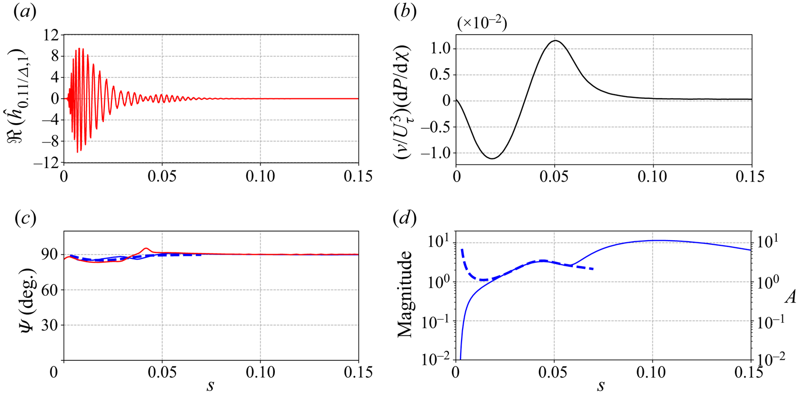
Figure 4. Curvilinear evolution of (a): the optimal roughness. (b) The streamwise pressure gradient made non-dimensional with the friction velocity  $U_\tau = (\nu \partial _\eta U_{\chi }(\eta =0))^{0.5}$ and kinematic viscosity $\nu$. (c) The $\varPsi$ angle of the optimal roughness (red) and response (blue). (d) The magnitude of the optimal response. The optimal perturbation obtained with the global resolvent (solid line) and the mode calculated by a local stability analysis (dashed line) are represented.
The real part of the optimal roughness is plotted in figure 4(a). Its amplitude is close to zero at both extremities of the domain and reaches its maximum magnitude at  $s\approx 0.008$. It also has a second (weaker) local maximum at $s=0.05$, with a second amplification region starting at $s=0.04$. The curvilinear evolution of the $\varPsi$ angle of the optimal roughness is represented in red in figure 4(c). We observe that it remains close to $90^\circ$ on the whole domain, with small variations up to $s=0.04$. Concerning the optimal perturbation, the magnitude of the mode as a function of $s$ is plotted in figure 4(d). The magnitude $d_{\boldsymbol {\hat {u}}}(s)$ is defined as $d_{\boldsymbol {\hat {u}}}(s)=\sqrt {\int _0^{L_\eta } \| \boldsymbol {\hat {u}}(s,\eta ) \|^2 \, \textrm {d} \eta }$, where $L_\eta =45\varDelta$. We notice a weak magnitude at $s=0$, a strong amplification from $s=0$ to $s=0.01$, a decrease around $s=0.05$ and finally a second amplification from $s=0.057$ up to $s=0.1$. The evolution according to $s$ of its $\varPsi$ angle is displayed in blue in figure 4(c) and we also notice a value close to $90^\circ$ on the whole domain. Figure 4(b) represents, as a function of $s$, the pressure gradient scaled using $U_\tau = (\nu \partial _\eta U_{\chi }(\eta =0))^{0.5}$ and $\nu$. In the ONERA-D case, the streamwise pressure gradient is negative up to $s=0.035$, then positive until the limit of the domain, with a flattening around $s=0.09$. This pressure-gradient changeover is typical of a flow on a swept wing and leads to the existence of two inflection points in the CF velocity profile for some values of $s$ (Reference Arnal and CasalisArnal & Casalis 2000; Reference Wassermann and KlokerWassermann & Kloker 2005). A negative pressure gradient is favourable to the development of CF waves, which accounts for the increase in the magnitude of the response at the beginning of the domain, while a positive pressure gradient is generally responsible for the growth of TS waves. Additional results about the base flow for a configuration close the current one are presented in Reference Kitzinger, Leclercq, Marquet, Piot and SippKitzinger et al. (2023).
Based on the characteristics of the optimal response, namely a high magnitude at the leading edge but not in the close vicinity of the AL and a  $\varPsi$ angle close to $90^\circ$, we can conclude that the optimal response is a CF-type mode. This is consistent with previous observations of the modes appearing in the case of swept wings with wall roughness (Reference Saric, Reed and WhiteSaric et al. 2003). Moreover, the fact that, having an identical spanwise wavenumber, the optimal roughness and the associated perturbation have an almost equal curvilinear evolution of the $\varPsi$ angle shows that they also have a very close evolution of their curvilinear wavenumber $k_s(s)$, as observed by Reference Tempelmann, Hanifi and HenningsonTempelmann et al. (2012a).
A direct link between the double amplification of the optimal roughness and the associated response was not identified. Indeed, when calculating the response associated with a roughness height equal to the optimal roughness height for  $s<0.04$ and to $0$ beyond, the same second amplification was observed. This is also shown by the roughness studied in § 5.2.1.
We now compare the magnitude and the  $\varPsi$ angle of the optimal response with the results obtained using a local stability analysis (figure 4c,d). The local stability analysis considers eigenmodes sought in the $(s,\eta,z)$ reference frame under the form $q=\hat {q}(\eta )\, \textrm {e}^{\textrm {i}(\alpha s + \beta z - \omega t)}$. The spatial stability analysis in the $s$-direction is solved for fixed $\beta$ and $\omega$ real values. The local stability code solves the one-dimensional differential eigenvalue problem with a high-order scheme. The parallel flow assumption is used, and the flow computed by the boundary-layer solver is used as the base flow, to avoid interpolation errors from the finite-element-method (FEM) mesh. In the local stability analysis framework, the $\varPsi$ angle is directly derived from the real parts of $\alpha$ and $\beta$ and the knowledge of the inviscid streamwise direction at each chordwise location. The spatial amplification $A(s)$ is represented in figure 4(d) and is defined as $\ln (A(s)/A_0)=\int _{s_0}^s-\Im {(\alpha (s))}\, \textrm {d} s$ (see for instance Reference Arnal and CasalisArnal & Casalis (2000) and Reference Reed, Saric and ArnalReed, Saric & Arnal (1996) for reviews on local stability approach) with the initialisation at $s_0=0.003$ and $A_0$ arbitrarily chosen such that $A(s)$ fits the magnitude of the optimal response. We observe that the $\varPsi$ angle and the amplification for $0.018< s<0.056$ match very well. For $s<0.013$, the mismatch is due to the fact that the optimal response is triggered by a roughness, which is not taken into account in the spatial stability analysis. The position of the beginning of the growth phase is the position of branch I and coincides closely with the maximum magnitude of the associated roughness ( $s=0.008$). This is in good agreement with the literature (Reference ChoudhariChoudhari 1994; Reference Tempelmann, Hanifi and HenningsonTempelmann et al. 2012a; Reference Sipp and MarquetSipp & Marquet 2013). Finally, the second amplification of the mode from the transfer function analysis ( $s>0.057$) could not be captured by the local stability analysis. This may be due to several reasons. First, the second amplification may be caused by a non-modal spatial growth, which is not captured by examining only the most unstable mode of the local stability analysis. Secondly, the assumptions of flow parallelism and no surface curvature used in the local stability analysis are also limiting and may account for this deviation. It is not obvious whether a PSE method, which takes into account weak non-parallelism but does not capture non-modal mechanisms (Reference Towne, Rigas and ColoniusTowne et al. 2019), would be able to recover this second amplification.
The evolution of the curvilinear wavenumber  $k_s$ with respect to $s$ is represented in figure 5 and the position of the maximum magnitude of the optimal roughness is indicated with a green vertical dashed line. The wavenumber $k_s$ decreases from the AL until $s=0.03$, where $k_s\varDelta =0.16$. At the location of maximum magnitude $s=0.008$ we get $k_s\varDelta =0.32$. Afterwards, it reaches a local maximum of $k_s\varDelta =0.25$, where the second amplification region begins and is then approximately $0.22$ up to the end of the domain. Moreover, since the spanwise wavenumber is fixed and $\varPsi \approx 90^\circ$ on the whole domain, the curvilinear evolution of $k_s$ is closely related to the orientation of the external streamlines.
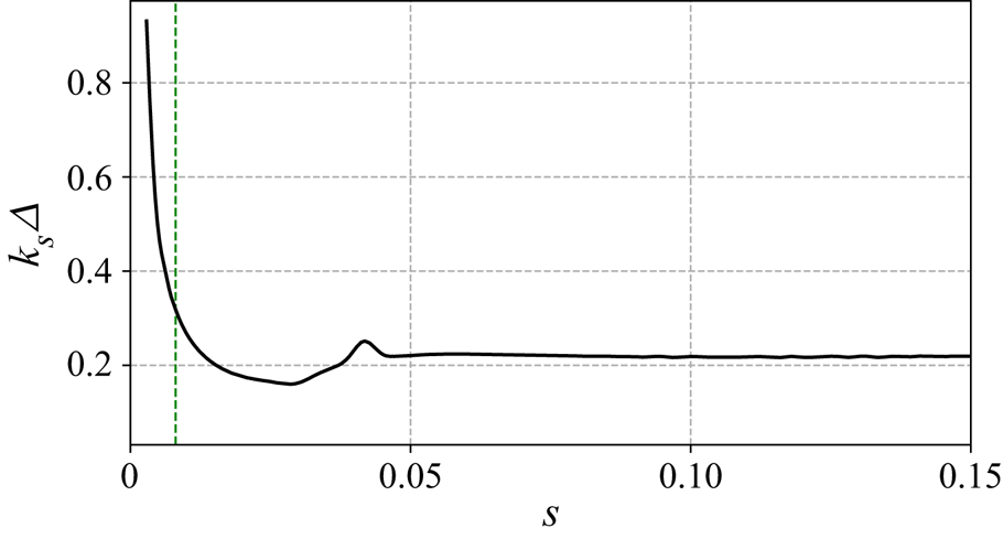
Figure 5. Curvilinear evolution of  $k_s\varDelta$ of the optimal roughness with $\beta \varDelta =0.11$. The location of the maximum magnitude of the optimal roughness is shown (green vertical dashed line).
5.1.2 Optimal roughness and perturbations for $0.05 \le \beta \varDelta \le 0.3$

The optimal roughness for  $\beta \varDelta \in [0.05,0.3]$ has qualitatively similar spatial structures as the one at $\beta \varDelta =0.11$ with two magnitude maxima and zero values at the extremities of the domain as well as a curvilinear wavenumber which varies with $s$.
$s$.
In figure 6(a) we plot, according to  $\beta \varDelta$, the positions of the maximum magnitude of the optimal roughness and perturbation for the different spanwise wavenumbers. Concerning the optimal roughness, the position of the maximum tends to get further away when increasing $\beta \varDelta$, moving from $s\approx 0.006$ to $s\approx 0.016$. For all spanwise wavenumber values, the optimal roughness is located relatively close to the AL, thus corroborating the conclusions of previous studies (Reference Radeztsky, Reibert and SaricRadeztsky et al. 1999; Reference Thomas, Mughal and AshworthThomas et al. 2017). Contrary to the optimal roughness, the position of the maximum magnitude of the optimal response tends to get closer to the AL with the increase of the spanwise wavenumber, moving from $s=0.13$ for $\beta \varDelta =0.05$ to $s=0.022$ for $\beta \varDelta =0.30$.

Figure 6. (a) Curvilinear position of the maximum magnitude of the optimal roughness and response as a function of  $\beta \varDelta$. (b) Local $\varPsi$ angle of the optimal roughness and response at the location of the maximum magnitude. The values related to the optimal roughness and responses are respectively depicted by crosses and circles.
In figure 6(b) are represented the  $\varPsi$ angles of the optimal roughness and response at the curvilinear location of the maximum magnitude as a function of $\beta \varDelta$. We note that the $\varPsi$ angle remains almost constant with the evolution of the spanwise wavenumber, with values close to $90^\circ$.
These observations on the position of the maximum of the magnitude of the optimal response as well as on the value of the associated  $\varPsi$ angle tend to show that the optimal response is of CF type for $\beta \varDelta \in [0.05,0.3]$.
5.2 Flow response to specific roughness
In the present section, we assess the performance of the formulation (3.14) associated with the approximation (3.15) to reconstruct the response triggered by localised and non-localised roughness.
5.2.1 Case of square wave roughness localised in the curvilinear $s$-direction and harmonic in the spanwise $z$-direction


We consider a roughness periodic (characteristic size  $L_z=2{\rm \pi} /\beta _0$) in $z$ and which is compact (characteristic size $L_s$) and localised in the curvilinear direction (around $s_0$)
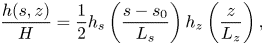 \begin{equation} \frac{h(s,z)}{H} = \frac{1}{2}{h}_s\left(\frac{s-s_0}{L_s}\right){h}_z\left(\frac{z}{L_z}\right), \end{equation}
where
 $$\begin{gather} {h}_{s} = {-}\mathcal{H}_{{-}1} + 2\mathcal{H}_{{-}3/4}-2\mathcal{H}_{{-}1/4} + 2\mathcal{H}_{1/4}-2\mathcal{H}_{3/4} + \mathcal{H}_{1}, \end{gather}$$
 $$\begin{gather}{h}_z = {-}1 + 2\mathcal{H}_{0} \mbox{ for } z\in [{-}1/2; 1/2[ \quad \mbox{and} \quad {h}_z(z + 1) = {h}_z(z) \quad \forall \, z, \end{gather}$$
where function  $\mathcal {H}_{\xi }$ refers to the Heaviside function with the discontinuity at $\xi$. The roughness exhibits a square wave shape of peak–valley distance $H$, and zero mean, both in the chordwise direction $s$ and the spanwise direction $z$. Its spanwise wavenumber $\beta _0$ is chosen so as to coincide with the most amplified spanwise wavenumber optimal roughness ( $\beta _0\varDelta =0.11$). We picked $L_s$ close to the local wavelength $L_s=2{\rm \pi} /k_s=2{\rm \pi} \varDelta /(k_s\varDelta =0.32)$ of this optimal roughness at its maximum magnitude occurring at $s_0=0.008$ (see figure 5). The roughness centred at $s_0=0.008 \approx 82 \varDelta$ is represented in figure 7. In the following, we will also consider this same roughness but moved around $s_0=0.016\approx 165 \varDelta$ and $s_0=0.056 \approx 577 \varDelta$: since we keep the same $L_s$, these roughnesses are no longer optimal with respect to the local optimal roughness wavenumbers, which are, respectively, $k_s\varDelta =0.19$ and $k_s\varDelta =0.22$ at these new locations.
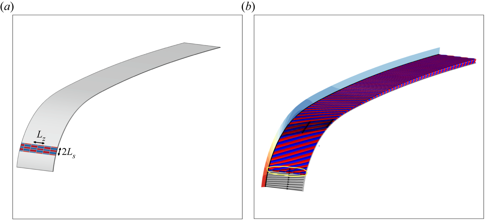
Figure 7. (a) Shape  $h(s,z)/H$ of the square wave roughness with $L_z/\varDelta =2{\rm \pi} /0.11\approx 57.1$ and $L_s/\varDelta =2{\rm \pi} /0.32\approx 19.6$ and localised at $s_0=0.008$. The positive and negative values are represented in red and blue, respectively. (b) Associated response calculated solving the LNSE with the same representation as figure 3. The yellow ellipse indicates the area where a difference with the response calculated using the approximation (5.4) occurs.
Equation (3.9a,b) for the wall roughness becomes  ${h}(s,z)=(H/2){h}_s((s-s_0)/L_s)\sum _{m=-\infty }^{+\infty } \hat {h}_{z,m}\, \textrm {e}^{\textrm {i} m\beta _0 z}$, where $\hat {h}_{z,m}$ is the Fourier transform of a zero-mean square wave, so that $\hat {h}_{z,0}=0$ and $|\hat {h}_{z,m}| \sim m^{-1}$.
Considering an approximation with the dominant singular value and four harmonics, (3.14) for the response provides the following explicit form of the flow response:
 \begin{equation} \frac{\boldsymbol{u}(x,y,z)}{H}\approx \sum_{m = 1}^{4}\Re \left(\hat{h}_{z,m}\sigma_{1,m} \left\langle\hat{h}_{1,m}(s),{h}_s \left(\frac{s-s_0}{L_s}\right)\right\rangle_w\boldsymbol{\hat{u}}_{1,m}(x,y)\, {\rm e}^{{\rm i} m\beta_0 z}\right). \end{equation}
The local mean fluctuation rate  $\langle \| \boldsymbol {u} \|\rangle _z(s,\eta )/H$ of the perturbation may then be obtained by an average of the kinetic energy in the spanwise direction, see (3.16).
We have considered three locations of the roughness in figure 8:  $s_0=0.008$ (blue), $s_0=0.016$ (red) and $s_0=0.056$ (green). They are represented in panel (a) along with the optimal roughness (black). In panel (b) we represent the curvilinear evolution of the maximum mean fluctuation rate $max_\eta \sqrt {\langle \| \boldsymbol {u} \|^2\rangle _z}/H$ of the response obtained by solving the exact (3.11) (dashed lines) and by using the approximation formula defined in (5.4) (solid lines). A good agreement between the responses is found downstream of the roughness. Hence, if the roughness is sufficiently small not to trigger transition in its vicinity (natural transition), the downstream evolution of the fluctuation rate is well captured by a few singular values/harmonics. The magnitude peak at the location of the roughness is more noticeable when the response has low energy, so that the maximum magnitude of the most critical roughness is still well captured by the low-rank approximation (5.4).
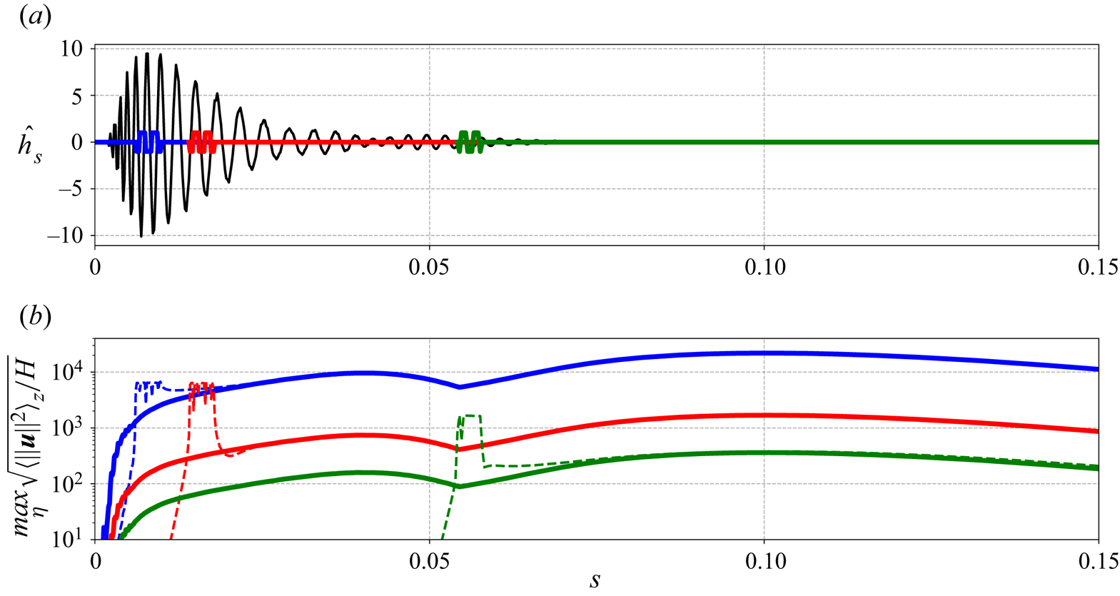
Figure 8. (a) Representation of the optimal roughness (black) and the shape of the square wave roughness  $h_s((s-s_0)/L_s)$ localised at $s_0=0.008$ (blue), $s_0=0.016$ (red) and $s_0=0.056$ (green) and $L_s/\varDelta \approx 18.5$. The square wave roughness in (a) have been magnified by a factor $2$ for visualisation purposes. (b) Curvilinear evolution of the maximum mean fluctuation rate $max_\eta \sqrt {\langle \| \boldsymbol {u} \|^2\rangle _z}/H$ of the responses by resolution of the (3.11) (dashed lines) and by using the approximation in (5.4) (solid lines).
Depending on the position of the roughness, the term  $\langle \hat {h}_{1,m}(s), {h}_s((s-s_0)/L_s)\rangle _w$ is modified. The latter is higher when the roughness is located where the optimal roughness has a strong magnitude and a similar curvilinear periodicity. That is why the response computed with (5.4) to the roughness positioned at $s=0.008$ has a maximum mean fluctuation rate of $2.2\times 10^4$ against $1.6\times 10^3$ and $3.5\times 10^2$ for the roughnesses at $s_0=0.016$ and $s_0=0.056$, respectively. The perturbation triggered by the roughness located at $s_0=0.008$ calculated by solving the LNSE is represented in figure 7. The only notable difference from the perturbation calculated with the approximation (5.4) is in the region of the roughness highlighted by the yellow ellipse, where the response exhibits a spatial structure similar to that of the roughness. Note that a PSE method would not be able to compute the perturbation in the vicinity of the roughness since it does not capture the non-modal mechanisms triggered by the roughness (which are well reproduced when solving the LNSE and accounted in the transfer function analysis by the sub-optimal modes).
5.2.2 Case of a compact roughness in both the curvilinear $s$- and spanwise $z$-directions


Considering again a roughness in separate form given by (5.1), we now choose
 $$\begin{gather} {h}_s(s) = \sqrt{1-s^2} \quad \textrm{for } s\in[{-}1,1] \quad \textrm{and}\quad {h}_s(s) = 0 \quad \textrm{for } |s|>1 \end{gather}$$
 $$\begin{gather}{h}_z(z) = {\rm e}^{{-}z^2}. \end{gather}$$
 Hence, the roughness is a Gaussian in the  $z$-direction localised around $z=0$ and a semi-ellipse localised at $s_0$ in the $s$-direction with the major axis being $L_s$ and the minor axis $He^{-z^2}/2$. We set $s_0=0.008 \approx 82 \varDelta$, $L_s/\varDelta =20.6$, $L_z/\varDelta =10.3$. The roughness shape $h/H$ is represented in figure 9(a) and can be considered as representative, for example, of the presence of an insect on a wing surface. The spatial structure of the response calculated solving the LNSE is shown in figure 9(b). The response develops from the position of the roughness and is convected downstream in the direction of the external streamlines where it acquires the spatial structure of a CF mode.
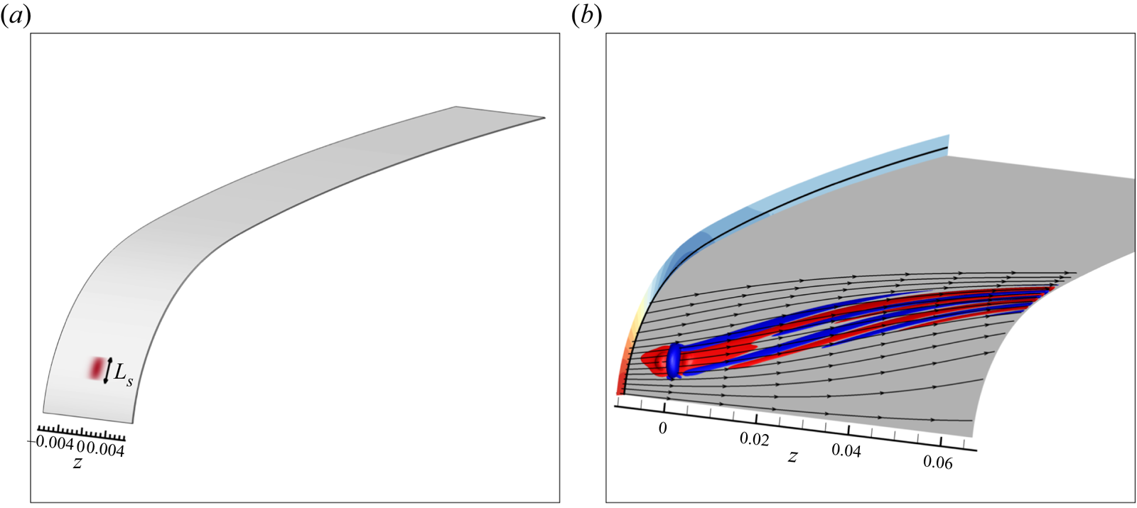
Figure 9. (a) Three-dimensional representation of the localised roughness  $h(s,z)/H$ with $s_0=0.008\approx 82 \varDelta$, $L_s/\varDelta =20.6$, $L_z/\varDelta =10.3$. (b) Spatial structure of the corresponding response calculated by solving the LNSE, with the same representation as in figure 3.
With (3.9a,b), the wall displacement reads  ${h}(s,z)/H=(1/2){h}_s((s-s_0)/L_s)\int _{-\infty }^{+\infty } \hat {h}_{z,\beta }\, \textrm {e}^{\textrm {i} \beta z} \, \textrm {d} \beta$, where $\hat {h}_{z,\beta }$ is the Fourier transform of a Gaussian wave, so that $\hat {h}_{z,\beta }=(L_z/2\sqrt {{\rm \pi} }) \exp (-(\beta L_z)^2/4)$. We then calculate the response of the system by using (3.14). We will, once again, make the assumption that the first singular value is sufficiently dominant to neglect the following ones. Moreover, only the roughnesses with spanwise wavenumber $|\beta \varDelta |<0.5$ are taken into account
 \begin{equation} \frac{\boldsymbol{u}(x,y,z)}{H}\approx \int_{0}^{{0.5}/{\varDelta}}\Re\left(\hat{h}_{z,\beta}\sigma_{1,\beta} \left\langle\hat{h}_{1,\beta},{h}_s\left(\frac{s-s_0}{L_s}\right) \right\rangle_w\boldsymbol{\hat{u}}_{1,\beta}(x,y)\, {\rm e}^{{\rm i}\beta z}\right)\,{\rm d} \beta, \end{equation}
and the integral is discretised with the extended Simpson's rule with steps of  ${\rm \Delta} \beta =0.001$.
In figure 10 we represent the curvilinear evolution of the wall normal maximum of the mean fluctuation rate  $max_{\eta }(\sqrt {\langle \|\boldsymbol { u}\|^2\rangle _z})/H$. The response calculated from (5.7) is plotted with a dashed line while the response computed from the resolution of (3.11) is drawn with a solid line. We observe, once again, a good agreement between both responses downstream of the roughness, with a second amplification at $s=0.054$ and two local maxima at $s=0.042$ and $s=0.1$ reaching, respectively, $19.5$ and $41$. As in figure 8, the fact that the maximum response magnitude is reached at the location of the roughness is related to the low energy of the response due to the strong stability of the flow configuration considered in this paper.


5.2.3 Case of chordwise and spanwise harmonic roughness
In this section, we consider a roughness of harmonic shape
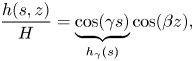 \begin{equation} \frac{h(s,z)}{H} = \underbrace{\cos(\gamma s)}_{{h}_\gamma(s)}\cos(\beta z), \end{equation}
with  $(\gamma,\beta ) \in \mathbb {R}^2$. The exact and approximated responses are respectively given by
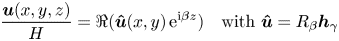 \begin{align} \frac{\boldsymbol{u}(x,y,z)}{H}& = \Re( \boldsymbol{\hat{u}}(x,y)\, {\rm e}^{{\rm i}\beta z}) \quad \mbox{with}\ \boldsymbol{\hat{u}} = R_\beta \boldsymbol{h}_\gamma \end{align}
 \begin{align} &\approx \Re(\sigma_{\beta,1}\langle\hat{h}_{\beta,1}(s),\cos(\gamma s) \rangle_w\boldsymbol{\hat{u}}_{\beta,1}(x,y)\, {\rm e}^{{\rm i}\beta z}) = \Re\left({\rm \pi} \sigma_{\beta,1} \overline{\hat{\hat{h}}_{\beta,1}(\gamma)} \boldsymbol{\hat{u}}_{\beta,1}(x,y)\, {\rm e}^{{\rm i} \beta z}\right), \end{align}
where  $\hat {\hat {h}}_{\beta,j}(\gamma )=({1}/{{\rm \pi} })\int _{0}^\infty {\hat {h}_{\beta,j}(s)}\, \textrm {e}^{-\textrm {i} \gamma s} \, \textrm {d} s$ is the Fourier transform of the $j$th symmetric optimal roughness $\hat {h}_{\beta,j}(s)$.
In figure 11 we represent, for each couple  $(\beta \varDelta,\gamma \varDelta )\in ([0,0.5]\times [0,1])$, the value of $max_{\eta,s}(\sqrt {\langle \|\boldsymbol { u}\|^2\rangle _z} )/H$ using (5.9). The same representation as figure 11 but considering (5.10) was also computed (not shown here) and gave similar results. This validates the approximation made in (5.10) and reveals that, when the roughness is not localised in the curvilinear direction, the maximum amplitude of the response is well calculated by the projection on the optimal roughness, and this for all values of $\beta$ and $\gamma$. Moreover, in the case of perturbations computed with the approximation (5.10), it is straightforward that the curvilinear position of the maximum represented in figure 11 is the same for all values of $\gamma$ and corresponds to the maximum of the optimal perturbation at the value of $\beta$ considered. Thus, in figure 11 we represent by black circles the curvilinear position at which the optimal perturbation reaches $max_{\eta,s}(\sqrt {\langle \|\boldsymbol {\hat {u}}_{\beta,1}\|^2\rangle _z} )/H$ for each value of $\beta \varDelta >0.03$.
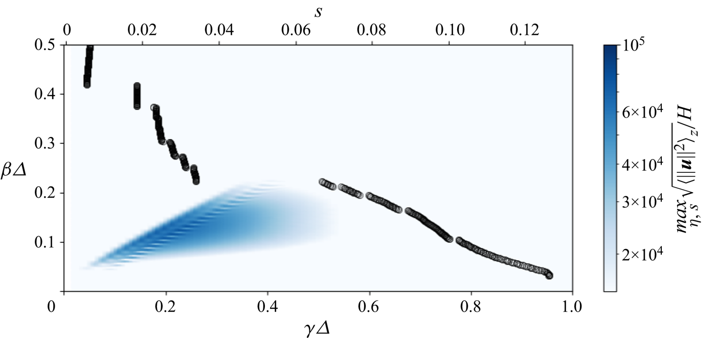
Figure 11. Representation, according to  $\beta \varDelta$ and $\gamma \varDelta$, of $max_{\eta,s}(\sqrt {\langle \|\boldsymbol { u}\|^2\rangle _z} )/H$. The curvilinear location where the maximum of the function for optimal perturbations is reached is plotted in black circles with respect to the top axis.
The spanwise wavenumbers  $\beta \varDelta$ associated with high values are between $0.05$ and $0.25$, which is directly related to the singular values $\sigma _1$ represented in figure 2. For a given spanwise wavenumber, the magnitude of the response is linked to the value of $\lvert \hat {\hat {h}}_{\beta,1}(\gamma )\rvert$. For example, for $\beta \varDelta =0.11$, a first maximum is reached at $\gamma \varDelta =0.18$ even if it does not correspond to the curvilinear wavenumber of the optimal roughness at its maximum magnitude ( $k_s\varDelta =0.32$ at $s=0.008$). However, this high value is justified by the fact that, as represented in figure 5, $\gamma \varDelta =0.18$ is close to the curvilinear wavenumber of the optimal roughness over a large range of $s$ values, including at positions where the roughness magnitude is high. Although $k_s\varDelta =0.32$ corresponds to the curvilinear wavenumber of the optimal roughness at its maximum magnitude, the strong variation of $k_s\varDelta$ at $s=0.008$ justifies the lower value of $\lvert \hat {\hat {h}}_{0.11/\varDelta,1}(0.32/\varDelta )\rvert$.
As the value of  $\beta$ increases, the most critical $\gamma$ values also increase. This is explained by the fact that, as shown in figure 6(a), the position of the magnitude maximum shifts downstream with increasing $\beta$, while remaining lower than the $s=0.016$ reached for $\beta \varDelta =0.3$. For increasing $s$, the direction of the external streamlines gets closer to the chordwise direction. Since the $\varPsi$ angle at the position of the maximum magnitude of the optimal roughness remains constant with increasing $\beta$ (figure 6b), the roughness also has a direction that approaches the chordwise direction at the location of its maximum magnitude. This implies an increase of $k_s$ at this position that is at least proportional to that of $\beta$, which explains the increase of the most critical $\gamma$ values in figure 11. Moreover, the position of the maximum varies from $s\approx 0.005$ for $\beta \varDelta =0.5$ to $s=0.126$ for $\beta \varDelta =0.03$. This evolution is slightly different from the one represented in figure 6 because we evaluate the maximum of different quantities. The ‘jumps’ that can be observed between different values of $\beta \varDelta$, despite the fact that the spatial structure of the optimal perturbations evolves continuously with $\beta$, is related to the presence of a ‘plateau’ in the curve of $max_{\eta }(\sqrt {\langle \|\boldsymbol {\hat {u}}_{\beta,1}\|^2\rangle _z} )(s)$ . The jump at $\beta \varDelta =0.22$ is linked to the switch from a position corresponding to the first amplification to a location related to the second amplification.
The overall picture indicates that the most dangerous roughnesses are characterised by  $\beta \leq 0.5 \gamma$, hence a rectangular trellis has elongated in the $z$-direction by an aspect ratio of at least $2$. The characteristic size of these roughness is around $\beta \varDelta \approx 0.1$, that is $L_z/\varDelta \approx 60$.
These calculations can be used to make a first attempt to predict the roughness height  $H_c$ for which nonlinear effects may appear. Some studies suggest that the first nonlinear effects appear in a three-dimensional flow when the magnitude of the disturbance velocity reaches approximately $10\,\%$ of the base-flow velocity (Reference Arnal, Casalis and HoudevilleArnal, Casalis & Houdeville 2008; Reference Tempelmann, Schrader, Hanifi, Brandt and HenningsonTempelmann et al. 2012b). Thus, considering the criterion $max_{\eta,s}\sqrt {\langle \|\boldsymbol {u}\|^2\rangle _z}/\sqrt {2}=0.1U^\infty$, we obtain, for a roughness with $\gamma \varDelta =0.18$, a critical height value of $H_c=4.92\times 10^{-6}\approx 4.9\,\%\varDelta$ for $\beta \varDelta =0.11$. It corresponds to the order of magnitude of the wall defects that can be encountered on real wings (Reference Radeztsky, Reibert and SaricRadeztsky et al. 1999). This is therefore a first indication that we could see nonlinear effects appear before the end of the domain in these flow conditions for unpolished aerofoils. For a roughness of height $H=4.92\times 10^{-6}$, the criterion is reached for $s=0.1$. It is important to note that this roughness size is small enough to allow the linearisation of the wall boundary condition to remain valid. Indeed, in our case, the displacement thickness $\delta ^*$ is greater than $10^{-4}$ and the approximation remains valid for roughnesses of height below $5\,\%\delta ^*$ (Reference Schrader, Brandt and HenningsonSchrader et al. 2009; Reference Tempelmann, Schrader, Hanifi, Brandt and HenningsonTempelmann et al. 2012b).
6. Conclusion
In this paper, we studied the receptivity of a swept aerofoil to wall roughness using a transfer function from wall displacement inputs to full velocity perturbations. An incompressible flow covering the whole leading edge was considered using a global framework. We have identified the most critical spanwise and curvilinear wavenumbers, as well as the spatial structure of the optimal roughness and associated perturbations. In the case of the spanwise wavenumber with the highest dominant singular value, the optimal response corresponds to a CF mode with two local maxima. The optimal roughness is located near the AL with a wavevector nearly orthogonal to the external streamlines. Moreover, the increase of the spanwise wavenumber shifts the location of the optimal roughness further downstream and the location of the optimal response closer to the AL. The most amplified curvilinear wavenumbers rise with increasing spanwise wavenumber. For all spanwise wavenumbers, the optimal roughness has a maximum magnitude close to the AL, confirming the results of previous studies (Reference Radeztsky, Reibert and SaricRadeztsky et al. 1999; Reference Tempelmann, Hanifi and HenningsonTempelmann et al. 2012a; Reference Thomas, Mughal and AshworthThomas et al. 2017). When the transfer function is low rank (few dominant singular values dominate), the optimal roughness and associated responses provide a low-order model. Once the optimal roughness and perturbations have been computed, the low-order model can be used to compute the flow response to any small-amplitude roughness shape, with only skinny and small-size matrix products, instead of the large-scale matrix inverse appearing in the definition of the transfer function.
Responses to various roughnesses (periodic and compact in both chordwise and spanwise directions) were finally computed. We verified that the magnitude of the response is the highest when the roughness has a Fourier transform involving spanwise wavenumbers corresponding to the highest singular values and curvilinear wavenumbers representative of the optimal roughness over a large range of  $s$ where its amplitude is high. Approximate responses calculated with a single singular value were compared with the responses obtained from the resolution of the LNSE and showed good agreement downstream of the roughness. When the roughness is localised in the curvilinear direction, a peak of magnitude can appear at the location of the roughness that cannot be captured by the low-rank method. In particular, this shows that the knowledge of the spatial structure of some optimal perturbations allows us to predict the characteristics of the response to a wide range of roughnesses. A first attempt to predict the height of a non-localised square wave roughness required to trigger nonlinear effects before $X=15\,\%$ was made. A critical roughness height around $10^{-6}$ was found for a square wave roughness with a spanwise wavenumber matching that of the most amplified optimal roughness. This size being of the order of the wall defect sizes that can be found on realistic aerofoils, it is a first indication of the possible transition before $X=15\,\%$ in this particular flow conditions. One possible prospect of this work is to apply the present analysis to configurations for which experimental or DNS results are available, such as those of Reference Reibert, Saric, Carrillo and ChapmanReibert et al. (1996) or Reference Tempelmann, Schrader, Hanifi, Brandt and HenningsonTempelmann et al. (2012b).
Supplementary material
Further details on underlying data are available from the corresponding author (E.K.).
Acknowledgements
The authors thank J.-P. Brazier for providing the local stability analysis code.
Funding statement
The study was supported by a grant from the Agence de l'innovation de défense (Defence Innovation Agency).
Declaration of interests
The authors declare no conflict of interest.


 Open access