AUGC sequences

Molecular biology revealed the structures of nucleic acid and proteins and provided a basis for handling genotypes and phenotypes by means of sound theoretical concepts. The notion of sequence space has been introduced for nucleic acidsReference Eigen⁵ and for proteins.Reference Maynard Smith⁶ The principle of sequence space construction is simple: A point ‘i’ is assigned to every sequence X_i and the Hamming distance, d_ij = d_H (X_i, X_j) serves as metric. (The Hamming distance counts the number of positions in which two aligned sequences differ.Reference Hamming^7, Reference Hamming⁸. It is identical with the minimal numbers of (single) point mutations required to convert one sequence into the other.) The properties of sequence space are illustrated best by means of a build-up principle: the sequence space is the set of all strings of length n over an alphabet of κ digits. may be constructed recursively by joining κ spaces of strings of length n − 1, (Figure 1). The construction principle is the same for any alphabet – binary, three-letter, four-letter – but the objects obtained are difficult to describe except in the case of binary sequences where is a hypercube of dimension n. Sequence spaces, in general, are high dimensional objects – the dimension is n × (κ − 1) – and low-dimensional, in particular two-dimensional, illustrations are frequently misleading. Two often misconceived features are: (i) all sequences in sequence space are (topologically) equivalent and hence they have the same number of neighbors – there are no sequences in the interior of ; and (ii) distances in high-dimensional spaces are small compared with those in low-dimensional spaces with the same number of nodes. A trivial but nevertheless important feature of sequence spaces is their connectedness. From every genotype we can reach every arbitrarily chosen genotype through a series of successive point mutations whose number never exceeds n or, in other words, the Hamming distance between two arbitrarily chosen sequences fulfils: d_H (X_i, X_j) ≤ n forall (X_i, X_j)∈ (independently of κ).

Figure 1 Sequence spaces. The properties of sequence spaces are illustrated by means of a recursive construction principle. The sequence space for strings of chain length n + 1, is constructed from two sequence spaces for strings of chains length n, , which are obtained by adding one symbol, (0 or 1) or (A or U or G or C), respectively, on the LHS to the string. Joining all pairs of sequences with Hamming distance d_H = 1 by a straight line yields the sequence space . The upper part of the figure deals with binary sequences: is a hypercube of dimension n. The lower part of the figure indicates the same construction for natural four letter sequences. The single digit element, which is a straight line (and one-dimensional) for binary sequences, is a tetrahedron (and three-dimensional) in the four digit case. The sequence space for two letter AUGC-strings is a tetrahedron of tetrahedra (middle), a fairly complicated looking object in six-dimensional space

Genotype–phenotype relations can be viewed as mappings from sequence space into a space of phenotypes S_n{S _.; d_S}, which comprises all possible phenotypes and has some distance measure d_S as metric. Fitness and other properties of phenotypes are thought to be expressed quantitatively by some function, f_k = Φ(S_j) where S_j is the phenotype formed by some genotype X_i : S_j = ψ(X_i). Fitness values are represented by real numbers, , with the common restriction to non-negative values.

The definition of genotype or sequence space is only a minor first step towards an understanding of genotype-phenotype relations. The complexity of phenotypes and additional influences through epigenetics and environmental factors is currently prohibitive for useful constructions of phenotype spaces for whole cells or organisms. There are, however, examples of simpler mappings from sequence spaces into phenotypes or structures that are currently accessible by theory as well as by experiment (see also the special issue of the Journal of Molecular Evolution, on Experimental EvolutionReference Lehmann⁹). We mention two of them: (i) in vitro evolution of biomolecules with predefined functions, in particular nucleic acid moleculesReference Joyce^10, Reference Klussmann¹¹ and proteinsReference Brakmann and Johnsson^12, Reference Jäckel, Kast and Hilvert¹³ and (ii) virus evolution.Reference Domingo, Parrish and Holland¹⁴ In both cases, the genotype is a polynucleotide that is short compared with the genoms of organisms. The numbers of possible genotypes in these relatively small sequence spaces are nevertheless huge compared with realistic population sizes: For chain lengths n > 40 the number of possible polynucleotide sequences exceeds Avogadro’s number, in protein sequence space this happens already at chain length n > 19. The enormous size of sequence spaces and the principal accessibility of every genotype by mutation, in essence, set the stage for evolutionary optimization.

Protein structures

Historically, the concept that protein folding follows a straightforward and reversible downhill process and ends at the thermodynamically stable (and therefore uniquely characterized) conformation of the molecule was derived from early work on the protein bovine pancreatic ribonuclease A.Reference Raines^18, Reference Marshall, Feng and Kuster¹⁹ The sequence of the small protein with a chain length of 124 amino acids was determined by Stanford Moore and William SteinReference Smyth, Stein and Moore^20, Reference Moore and Stein²¹ and only four years later the three-dimensional molecular structure of the protein had been determined.Reference Kartha, Bello and Harker^22–Reference Kim, Varadarajan, Wykoff and Richards²⁵ The major breakthrough in understanding folding of ribonuclease A came from the work by Christian Anfinsen:Reference White^26–Reference Anfinsen²⁹ the protein was denatured through breaking four disulfide bonds by reduction and complete unfolding. On oxidation with air the molecule returned to its native conformation in extremely high yields. Anfinsen cast the findings on ribonuclease A folding and unfolding into three criteria called the thermodynamic hypothesis of protein structure: (i) uniqueness – the sequence has only one conformation of minimum free energy (m.f.e.) and no other energetically nearby lying state; (ii) stability – small changes in the surrounding environment cannot result in substantial changes in the m.f.e.-conformation; and (iii) kinetic accessibility – a smooth free energy path leads from the unfolded random coil to the folded state. In essence, a two-state model considering a folded and an unfolded state of the molecule is sufficient to describe the observations. In more recent years the kinetics of the catalytic mechanism of ribonuclease A has been studied in detail.Reference Park and Raines³⁰ The most beautiful results obtained for ribonuclease suffer from the fact that biomolecules behaving like ribonuclease are rather a small minority in the universe of proteins. As a matter of fact, the majority of natural and artificial proteins behave differently and all three criteria of the thermodynamic hypothesis are rarely fulfilled. A stable protein structure requires a subtle balance between hydrophilic and hydrophobic interactions and, accordingly, the sequences from large sections of protein sequence space fail to from structures, because the polypeptides aggregate and the aggregates are insoluble in aqueous solution. Membrane proteins are an exception because they adopt their structures in a natural hydrophobic environment (for a review of the state of the art in membrane protein structure analysis see, for example, Ref. Reference Elofson and von Heijne31). Understanding protein structure and prediction of structures from known sequences turned out to be extremely hard, remained a major issue of biophysics for more than 30 years, and is still one of the hot topics.

In the late 1980s a new concept for the interpretation of protein folding was developed, which made use of an energy landscape.Reference Onuchic, Luthey-Schulten and Wolynes^32, Reference Dobson, Šali and Karplus³³ The energy of the protein is plotted upon conformation space of the protein sequence. Conformation space is commonly continuous in chemistry; the coordinates are all bond lengths, bond angles, and dihedral angles that determine the structure of the molecule.³⁴ The notion of an energy landscape describing energy as a function of the coordinates of a molecule is a result of the Born–Oppenheimer approximation in quantum mechanics, which separates the motions of fast-moving electrons and slow nuclei. Accurate energy landscapes are accessible through computation for small molecules and small molecular aggregates. As more and more data become available, the empirical reconstruction of free energy landscapes of proteins at atomic resolution becomes within reach.Reference Vendruscolo and Dobson³⁵ The numbers of degrees of freedom in conformation space are also hyperastronomical: considering only dihedral angles – in other words keeping bond lengths and bond angles constant – we estimate for a the chain length of ribonuclease A, n = 124, some 10⁹⁰ angular degrees of freedom leading to about 10¹⁵⁰ local minima of the energy landscape. LevinthalReference Levinthal^36, Reference Levinthal, Debrunner, Tsibris and Münck³⁷ formulated a paradox in view of these huge numbers of degrees of freedom: how can a protein manage to find the native conformation in a time interval as short as a millisecond when sequential sampling of conformation, one every picosecond, would take longer than the age of the universe? The answer is sketched in Figure 2: the folding landscape has the shape of a funnel, under folding conditions (almost) all random coil conformation have conformations of lower free energy in the neighborhood, a enormous large number of trajectories leads to the target conformation, and hence only a negligibly small fraction of conformation space is sampled along an individual trajectory. The Anfinsen funnel (Figure 2, left-hand side) describes the idealized case of a fast folding protein such as ribonuclease A, whereas most proteins are characterized by a rugged folding landscape with a great number of local (free) energy minima (Figure 2, right-hand side). Many proteins need assistance for folding that is provided in vivo by chaperonins being large protein assemblies with cavities, inside which the unfolded protein finds its way into the native conformation.Reference Horwich, Fenton, Chapman and Farr³⁸

Figure 2 Energy landscapes of protein folding. The sketch of the landscape on the LHS corresponds to the Anfinsen dogma of protein folding: The unfolded random coil of the polypeptide sequence is converted smoothly into the unique and stable native structure as observed with ribonuclease A. The sketch of the folding funnel on the RHS represents the more common case as observed with most proteins [Onuchic et al., 1997]: The native structure is reached via various intermediates that are represented by molten globules, sometimes long lived glassy states and (discrete) suboptimal conformations, which act as folding traps. The abscissa axis in both sketches is an appropriate cross section of conformational space. The factor Q is the fraction of native like contacts. Typically Q = 0.3 for molten globules, Q = 0.6 in the transition region and Q = 0.7 in the range of glass transitions. ‘Entropy’ and ‘energy’ are put in quotation marks because they are just illustrations implying that a wide funnel sustains a larger ensemble of trajectories leading to the target state, and the depth of the funnel is a measure of the stability of the native state. The majority of entropic contributions is not encapsulated in the width of the funnel and commonly the quantity on the ordinate axis is not pure energy but Gibbs’ free energy lacking entropy contributions from these degrees of freedom that are illustrated on the abscissa axis

In essence, the mechanism of protein folding is understood by now.Reference Onuchic, Luthey-Schulten and Wolynes^32, Reference Dobson, Šali and Karplus^33, Reference Dill, Ozkan, Shell and Weikl^39, Reference Service⁴⁰ Conventionally, protein structure is described at four hierarchical levels: primary, secondary, tertiary, and quaternary structure. The primary structure is the amino acid sequence of the polypeptide chain, the secondary structure consists of regular structural elements formed through closure of hydrogen bonds of the polypeptide backbone, the tertiary structure is the 3D structure of a protein or a protein subunit and the quaternary structure, eventually, provides information on the numbers and spatial arrangement of protein subunits.⁴¹ Two notions of structural units of proteins are used in addition to the presented classification of structure: (i) A protein domain consists of a part of protein sequence that can fold, exist, function, and evolve independently of the rest of the protein. Domains are highly variable with respect to chain lengths, which are typically lying between 25 to 500 residues. (ii) A structural motif is a structural 3D element or fold within the polypeptide chain, which is transferable from one protein to other proteins. In folding, the polypeptide chain passes a series of stages: (i) local interactions, in particular nuclei of α-helices and β or reverse turns, are introduced into the random coil at one of many – more or less equivalent – positions; (ii) secondary structures grow until about 30% of the contacts in the native state have been established and the molecules form a so-called molten globule – a partially ordered structure with still substantial flexibility; (iii) further loss of conformational freedom induces transitions to more rigid states – sometimes of glassy nature; and (iv) confinement to one of the narrow deep values corresponding either to the native structure or to one of the suboptimal conformations, which are usually inactive and therefore addressed as misfolded states. Conversion from a suboptimal state to the native conformation may be fast or slow depending on the barrier separating the valleys. In is commonly assumed that an ordered and rigid structure is required for efficient catalysis, a recent protein engineering study, however, produced a molten globule with perfect catalytic performance that is practically the same as that of the natural counterpart.Reference Vamvaca, Vögeli, Kast, Pervushin and Hilvert⁴² Prediction of protein structure from a known sequence is still a very hard task. Progress is regularly monitored every two years by Critical Assessment of Techniques for Protein Structure Prediction (CASP) contests: the two latest prediction evaluation meetings of the committees were CASP 6 and CASP 7.Reference Lattman^43, Reference Trapane and Lattman⁴⁴ The progress within the last two years has been modest but two changes were significant: (i) the gap between human prediction groups and automatic servers has been closed, and (ii) an improvement has been observed with template-based models resulting from the usage of multiple templates, template free modeling in regions where no template is available, and refinement.

Nucleic acid structures

Folding of random coil polynucleotide chains into DNA and RNA structures has been studied less frequently by far than protein folding – there are more than 40,000 protein-only structures in the Protein Data Bank compared with 575 deposited RNA-only structures. Nevertheless, the current understanding of nucleic acid structures is not far behind our knowledge on proteins. This has mainly three reasons: (i) nucleic acids are polyelectrolytes and hence almost always soluble in water; (ii) the structures of nucleic acids fall into two distinct classes, double helical duplexes and single stranded structures; and (iii) the dominant contribution to the stability of structures is the interaction of base pairs in double helical stacks. Indeed, formation of stacked base pairs is the major driving force for folding single stranded nucleic acid molecules into structures as it is for the formation of duplexes. Although DNA in nature is almost always double stranded and RNA mostly single stranded, both nucleic acids can and do exist in both forms. Examples are deoxyribozymes that are single-stranded catalytically active DNA molecules,Reference Breaker⁴⁵ double-strand RNA viruses, and double-stranded RNA in regulation of gene expression through RNA interference.Reference McManus and Sharp⁴⁶ The most important issue of double stranded DNA is the sequence dependence of double helical (B-DNA) structures, which is the key to protein recognition. Empirical data based duplex structure prediction from known local DNA sequences has been successful.Reference Packer, Dauncey and Hunter^47–Reference Gardiner, Hunter, Packer, Palmer and Willett⁴⁹ Important issues of higher order structures in cyclic DNA concern supercoil, catenation, and other topological properties.Reference Benham and Mielke⁵⁰ In this review, we shall not discuss duplex structures further but concentrate on conformations of single strand (RNA) molecules.

Polyelectrolytes require counter ions, which influence structure, and accordingly the structures of nucleic acids depend on ionic strength as well as the nature of the ions. This has been known from the early days of modeling DNA double helical structures from fiber diffraction data, and turned out to be particularly important for most full RNA structures, which are formed only when divalent Mg^2⊕ is present in the solution. Metal ions are also known to occur as elements of protein structure – a well known example is Zn^2⊕ in zinc fingersReference Klug and Rhodes^51, Reference Klug⁵² – but more frequently they play an essential part in the catalytic function of proteins. Like in proteins, RNA structures can be partitioned into primary, secondary, tertiary, and quaternary structure elements. The primary structure is the nucleotide sequence, the secondary structure, in essence, is a listing of Watson-Crick and GU wobble base pairs and consists of a small number of motifs that can be combined with few restrictions only, the tertiary structure comprises additional interactions in RNA structure, which place the secondary structure elements in 3D space. These interactions are often characterized as tertiary structural motifs. Commonly, the introduction of tertiary interactions keeps secondary structures unchanged but in rare cases tertiary structure formation causes secondary structure rearrangements.Reference Wu and Tinoco⁵³ The quaternary structure is defined as in proteins but plays only a minor role except in RNA protein complexes, for example in virions or cellular complexes like the ribosome.

RNA structure analysis and prediction is facilitated by the existence of motifs at all structural levels.Reference Moore^54–Reference Holbrook⁵⁶ Secondary structure motifs fall into four classes (Figure 3): (i) stacks, (ii) loops, (iii) joints, and (iv) free ends. In essence, the stacks provide the (only) stabilizing contributions to RNA structure, whereas the other elements are accompanied with positive free energy contributions. Loops are single-stranded elements attached to stacks, a hairpin loop to a single stack, a bulge or an internal loop to two stacks and a multi-loop to three or more stacks. Small hairpin loops commonly lead to large positive free energy contributions, because several degrees of freedom are frozen when the loop is closed. Exceptions, among others, are especially stable tetraloops, where a favorable geometry allows for additional base stacking.Reference Antao, Lai and Tinoco^57, Reference Antao and Tinoco⁵⁸ Joints are single strands combining two otherwise independent motifs – in case the joint is cut the RNA is partitioned into two unconnected molecules. Free ends, eventually, are single stranded stretches at the 5′-end or the 3′-end of the RNA molecule. Joints and free ends are characterized by high conformational flexibility. As in proteins, composite motifs are also found in RNA. As an example we mention the kink-turn motif,Reference Klein, Schmeing, Moore and Steitz⁵⁹ which is a combination of two stacks and a bulge or an internal loop between them. For certain constraints on loop size and RNA sequence the result is a sharp turn of the ribose-phosphate backbone and an acute angle formed by the axes of the double helices. The conventional definition of RNA secondary structure excludes pseudo-knots (see Figure 4 and the next section). RNA secondary structures are much more important than protein secondary structures, because every nucleotide is contained in a secondary structure motif and secondary structure formation commonly covers the major part of the free energy of folding.

Figure 3 Modules of RNA secondary structures. Stacks (blue) consist of base pairs combined in Watson-Crick-type double helices. Hairpin loops (red) terminate stacks, bulges and internal loops (pink and magenta) are adjacent to two stacks, and multiloops (violet) combine three or more stacks. A joint (brown) is an element joining two otherwise independent parts of the structure and free ends (orange) are mobile single strands at the 5′- and/or the 3′-end of the RNA. Below the conventional representation of the secondary structures we show an equivalent representation of structures by parentheses and dots: parentheses symbolize base pairs – the opening parenthesis is nearer to the 5′-end, the closing parenthesis is nearer to the 3′-end – and the dots stand for unpaired nucleotides. As with sequences the 5′-end is on the LHS, the 3′-end on the RHS of the parentheses string. The assignment of parentheses to base pairs follow the mathematical notation

Figure 4 Pseudo-knots in RNA structures. Pseudo-knots are structures with Watson–Crick base pairs that cannot be cast into the parentheses representation without violating the mathematical notation. Parentheses cannot be assigned unambiguously to the base pairs without usage of colors. The figure sketches hairpins from two classes: (i) an hairpin-type (H-type pseudo-knot) (LHS) where a hairpin is involved in downstream base pairing, and (ii) the kissing loops motif (RHS) involving two hairpin loops forming a stack. Colored parentheses representations are shown below the figures

Tertiary motifs are larger in number and richer in diversity than secondary structure motifs.Reference Holbrook⁵⁶ A systematic nomenclature of base pairs allows for a classification of non-Watson-Crick type nucleotide-nucleotide interactionsReference Leontis and Westhof⁶⁰ The search for tertiary RNA motifs has been very successful so farReference Leontis and Westhof^61–Reference Lescoute and Westhof⁶³ and is still continued on a worldwide basis.Reference Leontis, Altmann, Berman, Brenner, Brown, Engelke, Harvey, Fabrice Jossinet, Lewis, Major, Mathews, Richardson, Williamson and Westhof⁶⁴ The most common and overall structure dominating motif is end-to-end base pair stacking of helices, also called continuous interhelical base stacking (COIN stacking). It combines stacks into elongated double helical stretches. A well known example is found in tRNAs – the 3D structure was first determined for phenylalanyl-tRNA (tRNA^phe)Reference Rich and RajBhandary⁶⁵ – where the stacks terminated by the dihydro-U-loop and the anticodon loop form one extended helix and so do the stack of the TΨ-loop and the terminal stack carrying the CCA-end. The ‘L’-shaped tRNA structure is stabilized by four Mg^2⊕ ions binding to specific sites and a number of tertiary interactions involving a pseudo-knot, non-Watson-Crick base pairs, base intercalation, and binding to 2′-OH of the ribose moieties (Figure 5). Studies on randomized genes have shown that the reverse-Hogsteen base pair bridging the TΨ-loop (T54 = A58) is essential for the rigid and strong contact between the dihydro-U- and the TΨ-loop, and that the base pair is needed together with other interactions for the maintenance of the ‘L’-shape.Reference Zagryadskaya, Kotlova and Steinberg⁶⁶

Figure 5 Tertiary interactions in tRNA structures. The figure on the LHS shows the conventional cloverleaf secondary structure of phenylalanyl transfer RNA (tRNA^phe). Continuous interhelical base (COIN) stacking shapes of the molecule into an ‘L’. The stack closed by the dihydro-U-loop (green) associates end-on-end with the anticodon stack (red), the nucleotide between the two stacks, G26, forms a non-Watson-Crick base pair with A44. Similarly, the stack of the TΨ-loop (blue) is coaxial with the terminal stack (violet) with one regular AU base pair in between. Other tertiary interactions further stabilizing the ‘L’-structure are shown as broken grey lines

Kinetic folding of RNA molecules follows similar principles as does kinetic protein folding. The process is initiated by local folding of structural nuclei of stacks at several positions of the RNA sequence, then the stacks grow until they form the still flexible secondary structure. The introduction of tertiary contacts and the addition of Mg^2⊕ cations result in the full 3D structure of the molecule. Although the kinetic details of hairpin formation are quite involved,Reference Chen⁶⁷ the overall kinetics can be described well as a cooperative processReference Pörschke and Eigen^68–Reference Pörschke, Pecht and Rigler⁷⁰ and modeled by straightforward algorithmsReference Flamm, Fontana, Hofacker and Schuster⁷¹ or computed by Arrhenius kinetics.Reference Wolfinger, Svrcek-Seiler, Flamm, Hofacker and Stadler⁷² It is worth mentioning the highly promising single molecule techniques, which are steadily providing additional information on biopolymer structures and structure formation. Techniques successfully applied to RNA and protein folding are atomic force microscopy and fluorescence techniques.Reference Borgia, Williams and Clarke^73, Reference Li, Vieregg and Tinoco⁷⁴

RNA replication and mutation

The evolution of RNA molecules in the test tube represents the simplest system that fulfils the criteria for Darwinian evolution: (i) multiplication, (ii) variation, and (iii) selection. Evolutionary studies of RNA molecules in the test tube were initiated in the 1960s by Sol Spiegelman and his groupReference Mills, Peterson and Spiegelman^15, Reference Spiegelman¹⁶ and has remained a highly active field ever since.Reference Joyce^10, Reference Watts and Schwarz⁸⁰ The kinetics of RNA replication by means of viral replicases has been studied in great detail.Reference Biebricher, Eigen and Gardiner^81–Reference Biebricher, Eigen and Gardiner⁸³ Although RNA replication follows a complicated multistep reaction mechanism, the overall kinetics under suitable conditions consisting of excess replicase and nucleotide triphosphates can be described by simple exponential growth (Figure 6). In this phase, complementary replication sketched in Figure 7 can be represented by a simple two-step mechanism

()

Figure 6 RNA replication by viral replicases. The growth curve of RNA concentration in a closed system with polymerase and excess nucleotide triphosphates is shown.Reference Biebricher, Eigen and Gardiner⁸¹ In the exponential phase the total concentration of RNA is smaller than the total concentration of replicase, in the linear phase RNA is present in excess and, eventually at high RNA concentration the growth curve levels off, since the enzyme is bound in inactive RNA-replicase complexes and RNA synthesis is blocked by product inhibition

Figure 7 Complementary replication of RNA. Complementary replication consists of (i) duplex formation from single strands by template induced synthesis and (ii) dissociation of the duplex into a plus and a minus strand. The dissociation of the completed duplex is highly unfavorable because of the large negative free energy of duplex formation. Complex dissociation is facilitated by the enzyme, which separates the two strands on the fly in order to allow for independent structure formation and prevention of the formation of the complete duplex

The solution of the kinetic equations leads to two modes that describe fast internal equilibration and growth of the plus-minus ensemble with a rate parameter, , that is the geometric mean of the two rate constants:

()

with x ₊ = [X ₊] and x ₋ = [X ₋] being the concentrations of plus and minus strands, respectively. Variation is introduced into ensembles of replicating RNA molecules by unprecise copying or mutation. Three classes of mutations are distinguished: (i) single nucleotide mismatch in the replication duplex leading to a point mutation (Figure 8), (ii) duplication of part of the RNA sequence leading to insertion of nucleotides, and (iii) deletion of nucleotides.

Figure 8 Point mutation in replication of RNA. Point mutation results from a mismatch in the replication duplex. The figure sketches the result of a U-G mismatch that leads to a point mutation of transition type: A→G and U→C

A molecular theory of evolution based on the kinetics of replication and mutation has been formulated by Manfred Eigen.Reference Eigen⁵ The concept is based on the reaction network,

()

which is considered under the idealized conditions of excess nucleotide triphosphates and replicase. The rate parameter f_j refers to replications – correct and incorrect – of template X_j and the factor Q_ij represents the frequency of production of X_i as a copy of X_j. Since every copy has to be either correct or a mutant the conservation relation holds. The kinetic differential equations resulting from equation (4) with x_i = [X_i] are linear

()

and can be solved in terms of eigenvalues and eigenvectors of the selection-mutation matrix W, which can be factorized into a product of the mutation matrix Q and the diagonal matrix of replication rate parameters, F:

Since all sequences X_i can be reached from everywhere in sequence space by a chain of successive point mutations, the matrix W ^m has only strictly positive entries for sufficiently large m and the Perron-Frobenius theoremReference Seneta⁸⁴ holds: The eigenvector ζ₀ corresponding to the largest eigenvalue λ ₀ has exclusively strictly positive components and all mutants X_i are present in the population after some time: x_i(t) > 0 for t >> 0. The eigenvalue λ ₀ is positive and all components of the eigenvector are growing exponentially. The mutant distribution determined by the eigenvector ζ₀ is called quasi-species since it represents the genetic reservoir of an asexually replicating species. It is straightforward to introduce a constraint into equation (5) that limits population size asymptotically to lim_{t →∞}c(t) = c ₀:

()

Here, is the unit matrix and represents the mean replication rate parameter of the population. In the solutions of equation (5a) the population approaches indeed the stable stationary state , which is determined by the components of the eigenvector ζ₀. Choosing c ₀ = 1 yields relative or normalized concentrations: (which will be used in the rest of this section).

All entries of the mutation matrix Q can be derived from three parameters, the mutation rate p, the Hamming distance d_H (X_i, X_j), and the sequence length n, provided the uniform mutation rate model is adopted. This model is based on the assumption that mutation rates are independent of the position on the RNA sequence:

()

The rate parameters f_i are derived from the mappings Ψ and Φ from sequence space into shape space and into real numbers as formulated in equation (1).

In the absence of neutrality, the stationary distribution of sequences contains a master sequence, X _M, which is characterized in terms of the largest replication rate parameter: f _M = max{f_i∀i = 1,…, N}. At sufficiently small mutation rates p, the stationary concentration of the master sequence is largest, . A simple expression for stationary concentrations can be derived from the single peak model landscape. In this landscape, a higher replication parameter is assigned to the master and identical values to all others sequences: f _M = σ _M·f and f_i = f for all i ≠ M.Reference Swetina and Schuster^85–Reference Alves and Fontanari⁸⁷ The (dimensionless) factor σ_m is called the superiority of the master. The assumption leading to the single peak landscape is in the spirit of mean field approximations, since all mutants are lumped together into a single molecular species with average fitness. The concentration of the mutant cloud is simply and the replication–mutation problem boils down to an exercise in a single variable, x _M, the frequency of the master. A mean-except-the-master replication rate parameter is defined and then the superiority is of the form: . Neglecting mutational backflow we can readily compute the stationary frequency of the master sequence,

()

Non-zero frequency of the master requires Q _MM = σ _M⁻¹ > Q _min. Within the uniform error rate model an error threshold, defined by in the no mutational backflow approximation, occurs at a minimum single digit accuracy of

()

Figure 9 shows the stationary frequency of the master sequence, , as a function of the error rate. The exact solution of (5a) approaches the uniform distribution at mutation rates above error threshold. In other words, the concentrations of all molecular species in the population become identical. Such a state can never be achieved in real populations since population sizes N are always many orders of magnitude smaller than the numbers of sequences in sequence space – for a rather very large population size of N = 10¹⁵ the chain length at which sequence space matches population size is about n = 25. Accordingly, the no mutational backflow approximation as well as the exact solution of the differential equation (5a) fail to describe replication–mutation dynamics at mutation rates above the error thresholds because of finite population size effects (see later). The error threshold phenomenon is used in virology for the design of new antiviral drugs.Reference Domingo, Parrish and Holland^14, Reference Domingo⁸⁸

Figure 9 Error threshold in replication. The figure sketches the (relative) stationary concentration of the master sequence in the population as a function of the mutation rate . It vanishes at the error threshold in the ‘no mutational backflow’ approximation. The insert shows curves obtained as the exact solution derived from the largest eigenvector of the matrix W (red), by an approximation based on equal concentrations of all mutants that corresponds to the population at mutation rates p > p _max and becomes exact at p = 0.5 (blue), and by the no mutational backflow approximation (equation (7), black). The red curve and the blue curve approach each other above the error threshold and converge to the uniform distribution. The deterministic equation (5a) and its approximations fail to describe population dynamics at mutation rates above threshold. In addition, all replication processes in reality are bound by a minimum error rate, p _min, that represents the physical accuracy limit of replication

RNA secondary structures

An RNA secondary structure S of the sequence X = (a ₁, a ₂,…, a_n) where the nucleotides are chosen from an alphabet, e.g. a_i∈{A, U, G, C}, is a planar graph with the nodes being the individual nucleotides a_i. The edges, i·j∈S, are defined by the following criteria:

1. (i) for all nodes i≤(n − 1) holds i·i + 1 ∈ S (backbone),

2. (ii) for all nodes i exists maximal one k ≠ {i + 1, i − 1} such that i·k ∈ S (base pairs),

3. (iii) from i·j ∈ S and k·l ∈ S with k < l, and i < k < j follows i < k < l < j (no pseudo-knot rule), and

4. (iv) a criterion for structure formation, commonly minimization of free energy.

The backbone (i) represents the polynucleotide chain consisting of alternating phosphate and ribose moieties. The rule for base pairs (ii) defines all base pairs in structure S and excludes base triplets and other interaction involving more than two bases. The no pseudo-knot rule (iii) excludes structures shown in Figure 4. The m.f.e. condition, finally, defines the conditions under which S is as a possible structure of X. Thanks to these criteria the search for RNA secondary structures can be performed by means of dynamic programming.Reference Zuker and Stiegler^89–Reference Svobodová Vařeková, Bradáč, Plchút, Škrdla, Wacenovsky, Mahr, Mayer, Tanner, Brugger, Withalm, Lederer, Huber, Gierlinger, Graf, Tafer, Hofacker, Schuster and Polčík⁹³ Introducing the search for pseudo-knots into the search for optimal structures is possible in principle, but raises the computational demands enormously.Reference Rivas and Eddy⁹⁴ The situation with other tertiary motifs is similar. The currently used approach to predict tertiary structures starts from secondary structures and introduces tertiary contacts where sequence and structure make it possible.

Secondary structures can be represented as strings consisting of dots, and left and right parenthesis related by mathematical convention (Figure 3) without losing information. This fact provides an upper bound for the number of possible secondary structures: N_s(n) << 3ⁿ since acceptable mathematical parentheses notation is a severe restriction. Application of combinatorics yields a remarkably good approximation for sufficiently long sequences:Reference Schuster, Crutchfield and Schuster^78, Reference Hofacker, Schuster and Stadler⁹⁵

Accordingly, the number of sequences, N = 4ⁿ, is always larger – commonly much larger – than the number of secondary structures and we are dealing therefore with neutrality.

Folding RNA sequences into conventional secondary structures with minimal free energies provides a suitable model system for studying realistic sequence-structure maps of biopolymers for several reasons: (i) almost all RNA sequences form some base pairs and structures are found everywhere in sequence space, (ii) RNA folding follows a simple base pairing logic and hence it is accessible by mathematics and computation, and (iii) RNA secondary structures are physically meaningful and provide a basis for discussing RNA function. These three properties that are not fulfilled in the case of proteins, and the capability of multiplication in simple replication assays make RNA a suitable model for studies of evolution in vitro and in silico.

Neutrality and its consequences

The mappings defined in equation (1) provide the theoretical basis for both, rational and evolutionary design of biomolecules. Since we are dealing with orders of magnitude, more sequences than structures and a multitude of structures serving the same task, both mappings Ψ and Φ are non-invertible in the sense that many sequences form the same m.f.e. structure and many different structures may have the same function. The mapping Ψ is sketched in Figure 10. The inversion of the mapping S = Ψ(X) generally results in a set of sequences G(S) defining the pre-image of structure S in sequence space:

Figure 10 Neutral networks and compatible sequences. The set of sequences folding into the same m.f.e. structure S is denoted by G(S). It defines the nodes of the neutral network of structure S in sequence space. Connecting all pairs of sequences with Hamming distance d_H = 1 yields the neutral network Γ(S) (the graph drawn in red). A neutral network is embedded in the set of compatible sequences C(S), . A compatible sequence of structure S, X_C(S), forms S either as its m.f.e. structure or as one of its suboptimal conformations

()

It is a subset of the compatible set of structure S:⁹⁶. Since every sequence X_k maps onto some structure S_k, the union of all neutral sets covers the entire sequence space: .

Global properties of neutral networks can be derived from random graph theory.Reference Bollobás⁹⁷ The characteristic quantity for a neutral network is the degree of neutrality , which is obtained by averaging the fraction of Hamming distance-one neighbors that fold into the same m.f.e. structure, – with being the number of neutral single nucleotide exchange neighbors – over the whole network, G(S):

()

where |G(S)| is the number of sequences forming the neutral network. Connectedness of neutral networks, among other properties, is determined by the degree of neutrality:Reference Reidys, Stadler and Schuster⁹⁸

()

where . Interestingly, this threshold value depends exclusively on the number of digits in the nucleotide alphabet. Calculation yields the critical values λ _cr = 0.5, 0.423, and 0.370 for two, three, and four letter alphabets, respectively. Random graph theory predicts a single largest component for non-connected networks, i.e. networks below threshold, which is commonly called the giant component.

Real neutral networks derived from RNA secondary structures sometimes deviate significantly from the prediction of random graph theory. In particular, they can have two or four equally sized largest components. This deviation is readily explained by non-uniform distribution of the sequences belonging to G(S_k) over sequence space, which is caused by specific properties of the structure S_k.Reference Grüner, Giegerich, Strothmann, Reidys, Weber, Hofacker and Schuster^99, Reference Grüner, Giegerich, Strothmann, Reidys, Weber, Hofacker and Schuster¹⁰⁰ For example, structures that allow for closure of additional base pairs at the ends of stacks are more likely to be formed by sequences that have an excess of one of the two bases forming a base pair than by those with an ideally balanced distribution (n _G = n _C and n _A = n _U). For GC sequences the neutral network of such a structure is less dense in the middle part of sequence space (n _G = n _C) than above (n _G > n _C) or below (n _G < n _C), and we find two equally sized largest components, one at excess G and one at excess C.

Neutrality in sequence space has consequences for the selection process. The scenario of neutral evolution has been investigated in great detail by Motoo Kimura.Reference Kimura^101, Reference Kimura¹⁰² In the absence of differences in fitness values the distribution of neutral genotypes or sequences drifts randomly in sequence space until one particular genotype becomes fixed. Kimura’s theory yields two highly relevant results: (i) the average time of replacement of one genotype by another is the reciprocal rate of mutation, τ _subst = 1/p, and hence independent of population size, and (ii) the time of fixation of a mutant is proportional to the population size, τ _fix = 4N_e (with N_e being the effective population size). Neutrality can be introduced into model fitness landscapes, the corresponding selection-mutation equation (5a) is solved straightforwardly, and yields at the limit of small mutation rates for two sequences depending on the Hamming distance:Reference Schuster and Swetina¹⁰³

()

A pair of fittest neutral nearest neighbor sequences appears in the stationary mutant distribution strongly coupled at equal concentrations; two sequences, X_i and X_j, with Hamming distance d_H (X_i, X_j)=2 form a strongly coupled pair with a concentration ratio α/(1 − α); and for Hamming distance d_H (X_i, X_j) ≥ 3 the Kimura scenario holds: either of the two sequences is selected depending on initial conditions (and/or random fluctuations). The group of two or more neutral sequences that is selected is called the core of the quasi-species and replaces the master sequence of the non-neutral case. For more than two neutral nearest neighbor sequences the core of the quasi-species is derived straightforwardly: we consider the selection-mutation matrix W and neglect all terms O(ε ²). Without changing the eigenvectors of W we set f = f(1 − p)ⁿ and ε = 11, and obtain the adjacency matrix A. The core is then computed as the largest eigenvector of A. An example is shown in Figure 11. Increasing mutation rates p > 0 lead to small or moderate changes in the relative concentrations of sequences in the core, in fortunate cases ratios of concentrations hold almost up to the error threshold.

Figure 11 Neutral networks and quasi-species. An example of a quasi-species core for a degree of neutrality λ = 0.1. Fitness values f_i were assigned randomly to all 1024 binary (GC) sequences of chain length n = 10 with the constraint of 10% having the highest fitness value. The numbers on the sequences represent the decimal equivalent of the binary sequence, e.g. the two sequences X ₁₈₄ ≡ CCGCGGGCCC and X ₂₄₈ ≡ CCGGGGGCCC with Hamming distance d_H (X ₁₈₄, X ₂₄₈) = 1. The selected neutral network (upper part, LHS) comprises seven sequences. The relative concentrations in the limit of vanishing mutation rates, lim p→0, are given by the largest eigenvector of the adjacency matrix A (upper part, RHS): . As the computed curves show, the ratio of the individual stationary in the limit is also a good approximation for finite mutation rates almost up to the error threshold

Stochastic effects in RNA evolution

Stochasticity becomes important when particle numbers are small and this is certainly the case for rare mutations in evolution. For RNA molecules the number of possible single-point mutations is 3n, and this increases like binomial coefficients with the Hamming distance. A related source of stochastic effects concerns the smallness of all real populations compared to sequence space: in molecular evolution experiments, the numbers of RNA molecules in an experiment can hardly exceed 10¹⁵, which is practically nothing compared to 1.6 × 10⁶⁰, the number of sequences in and therefore quasi-species are always truncated at a certain distance from the population center.

Therefore, stochastic effects are particularly important in molecular evolution under several conditions:

1. (i) In the regime of sufficiently accurate replication the master sequence or the core of a quasi-species is surrounded by a cloud of mutants. Near the truncation distance from the population center mutations become very rare and the mutants cannot reach stationarity but remain fluctuating elements.

2. (ii) At mutation rates above threshold mutations to distant sequences gain sufficiently high probability to destroy inheritance and all mutants become equally frequent in the deterministic approach. Since the population cannot cover the whole sequence space, it spreads and starts to migrate through the sequence space.

3. (iii) Populations on neutral networks drift in the sense of Kimura’s neutral evolution. In particular, the population spreads and breaks up into different clones, which migrate through sequence space.

Scenarios (ii) and (iii) are similar but arise from two completely different origins: Scenario (ii) results from low accuracy that manifests itself in the elements of the Q-matrix and gives rise to migration of the population because of frequent mutations. The error threshold has been interpreted also as a localization threshold of the quasi-species in sequence space.Reference McCaskill¹⁰⁴ Scenario (iii) is tantamount to random drift in sequence space because of a degeneracy of the largest entries of matrix F.Reference Huynen, Stadler and Fontana¹⁰⁵

In order to simulate selection-mutation dynamics of RNA at the stochastic level, a realistic model based on chemical reactions in a flow reactor was conceived.Reference Fontana and Schuster^106–Reference Fontana and Schuster¹⁰⁸ The sequence-structure map is an integral part of this model in the sense that sequences are converted into m.f.e. secondary structures by means of an RNA folding mechanism. Structures are evaluated to yield replication rate parameters or fitness values f_i. The simulation tool starts from a population of RNA molecules and simulates chemical reactions corresponding to replication and mutation in a continuously stirred flow reactor (CSTR) by using Gillespie’s algorithm.Reference Gillespie^109–Reference Gillespie¹¹¹ In target search the replication rate parameter of a sequence X_i, f_i, is chosen to be a function of the distance between the m.f.e. structure formed by the sequence, S_i = f(X_i) and the target structure S_T,¹¹²

()

which increases when S_i approaches the target structure S_T (α is an adjustable parameter that was chosen to be 0.1). A trajectory is completed when the population reaches a sequence that folds into the target structure. Accordingly, the simulated stochastic process has two absorbing barriers, the target and the state of extinction. For sufficiently large populations (N > 30 molecules) the probability of extinction is very small; for population sizes reported here, N ≥ 1000, extinction has been never observed.

A typical trajectory is shown in Figure 12. In this simulation, a homogeneous population consisting of N molecules with the same randomly chosen sequence is applied as an initial condition. The target structure is the well-known secondary structure of phenylalanyl-transfer RNA (tRNA^phe, see Figure 5). The distance to target averaged over the entire population decreases stepwise until the target is reached.Reference Schuster, Crutchfield and Schuster^78, Reference Fontana, Schnabl and Schuster^107, Reference Fontana and Schuster¹⁰⁸ The process occurs on two timescales: Short adaptive phases are interrupted by long quasi-stationary epochs. Transitions between two structures S_i and S_j can be classified according to the nearness of their neutral networks G(S_i) and G(S_j).Reference Fontana and Schuster^113, Reference Stadler, Stadler, Wagner and Fontana¹¹⁴ Inspection of the sequence record during a quasi-stationary epoch on a given plateaus provides hints for the distinction of two scenarios:

Figure 12 A trajectory of evolutionary optimization. The topmost plot presents the mean distance to the target structure of a population of 1000 molecules. The plot in the middle shows the width of the population in Hamming distance between sequences and the plot at the bottom is a measure of the velocity with which the center of the population migrates through sequence space. Diffusion on neutral networks causes spreading on the population in the sense of neutral evolution.Reference Huynen, Stadler and Fontana¹⁰⁵ A remarkable synchronization is observed: at the end of each quasi-stationary plateau a new adaptive phase in the approach towards the target is initiated, which is accompanied by a drastic reduction in the population width and a jump in the population center (the top of the peak at the end of the second long plateau is marked by a black arrow). A mutation rate of p = 0.001 was chosen, the replication rate parameter is defined in equation (13), and initial as well as target structure are shown Table 1

1. (i) The structure is constant because of neutrality in the map Ψ and we observe neutral evolution. In particular, the number of neutral mutations accumulated is proportional to the number of replications on the population level. Evolution is a random walk of the population on a neutral network.

2. (ii) The process during the stationary epoch involves several structures with the same replication rate parameters. Because of neutrality in the map from structure to function, Φ, the population performs a kind of random walk in the space of neutral structures.

The random walk or the diffusion of the population on neutral networks is illustrated by the plot in the middle of Figure 12 showing the width of the population as a function of time.Reference Schuster, Crutchfield and Schuster⁷⁸ The population width increases during the quasi-stationary epoch and sharpens almost instantaneously after mutation has created a sequence that allows for the start of a new adaptive phase. The scenario at the end of the plateau corresponds to a ‘bottleneck’ of evolution. The bottom part of the figure shows a plot of the migration rate or drift of the population center in sequence space and confirms this interpretation: the drift is almost always negligibly slow unless the population center jumps from one point in sequence space to another point in sequence space where the molecule initiating the new adaptive phase is located. A closer look at the figure reveals the coincidence of three events: (i) collapse-like narrowing of the population width, (ii) jump-like migration of the population center, and (iii) beginning of a new adaptive phase.

In Table 1 numerical data obtained from sampling evolutionary trajectories under identical conditions¹¹⁵ are presented. The individual trajectories show enormous scatter in the time or the number of replications required to reach the target. Mean values and the standard deviations were obtained from statistics of trajectories under the assumption of a log-normal distribution. Despite the scatter three features are unambiguously detectable:

Table 1 Statistics of the optimization trajectories. The table shows the results of sampled evolutionary trajectories leading from a random initial structure S_I to the structure of tRNA^phe, S_T as target.Footnote * Simulations were performed with an algorithm introduced by Gillespie.Reference Gillespie^109, Reference Gillespie^110, Reference Gillespie¹²⁵ The time unit is here undefined. A mutation rate of p = 0.001 per site and replication was used. The mean and standard deviation were calculated under the assumption if a log-normal distribution that fits well the data of the simulations

* The following structures S_I and S_T were used in the optimization:

S_I: ((.(((((((((((((............(((....)))......)))))).))))))).))...(((......)))

S_T: ((((((...((((........)))).(((((.......))))).....(((((.......))))).)))))).....

1. (i) The search in GC sequence space takes about five time as long as the corresponding process in AUGC sequence space in agreement with the difference in neutral network structure.

2. (ii) The time from initial conditions to target decreases with increasing population size.

3. (iii) The number of replications required to reach the target from initial conditions increases with population size.

Combining items (ii) and (iii) allows for a clear conclusion concerning requirements in time and resources of the optimization process: fast optimization requires large populations whereas economic use of material and/or energy suggests working with small population sizes just large enough to avoid extinction.

Systematic studies on the parameter dependence of RNA evolution were reported in a recent simulation.Reference Kupczok and Dittrich¹¹⁶ Increase in mutation rate leads to an error threshold phenomenon that is closely to one observed with quasi-species on a single-peak landscape as described above.Reference Eigen, McCaskill and Schuster⁷⁷ Evolutionary optimization becomes more efficient¹¹⁷ with increasing error rate until the error threshold is reached. A further increase in the error rate leads to an abrupt breakdown of the success in optimization. As expected, the distribution of replication rates or fitness values f_i in sequence space is also highly relevant: a steep decrease of fitness with the distance from the fittest master sequence (forming the target structure) leads to the sharp error threshold behavior as observed with single-peak landscapes, whereas flat landscapes show a broad maximum of optimization efficiency without an indication of threshold-like behavior.

Beyond the one sequence–one structure paradigm

So far it has been assumed implicitly that every RNA sequence gives rise to one unique structure. This is almost always true when the notion of structure is restricted to a well defined thermodynamic or process determined folding criterion, m.f.e. or in situ folding during RNA synthesis. In general, the number of structures S_k that are compatible with a given sequence X are commonly quite large and form the set of compatible structures C(X), which consists of the m.f.e. structure together with all suboptimal structures. Efficient algorithms for the computation of suboptimal structures are available.Reference Zuker^118, Reference Wuchty, Fontana, Hofacker and Schuster¹¹⁹ Because the numbers of suboptimal structures are almost always too large to be computed, stored and retrieved, the computational procedures use restrictions: in Ref. Reference Zuker118, certain common but less important classes of structures are neglected, and in Ref. Reference Wuchty, Fontana, Hofacker and Schuster119 all structures are computed that lie within an predefined energy band above the m.f.e. (Figure 13). Alternatively, using the partition function of the states S_k, the superposition of all Boltzmann weighted structures can be calculated with little more computational effort than needed for the computation of the m.f.e. structure.Reference Hofacker, Fontana, Stadler, Bonhoeffer, Tacker and Schuster^91, Reference McCaskill¹²⁰ Yes-or-no pairing between two nucleotides is then replaced by a base pairing probability.

Figure 13 RNA structures. The m.f.e. structure of an RNA sequence is accompanied by a large number of suboptimal structures. The sequence GGCCCCUUUGGGGGCCAGACCCCUAAAGGGGUC folds into a single hairpin structure S ₀ with m.f.e. of −26.3 kcal/mole. The first suboptimal structure of this molecule, S ₁, is a double hairpin with a free energy of −25.3 kcal/mole. The figure shows the m.f.e. structure (LHS; red), the spectrum of suboptimal structures (middle; suboptimal conformations related to S ₀ are shown in red, those related to S ₁ in blue), and the barrier tree of the sequence (RHS) with two major basins for S ₁ (blue) and S ₀ (red)

Rules defining nearest neighbors in shape space and a measure of distance between structures are required for the construction of a free energy surface that identifies the (meta)stable conformations as local minima and the transitions states for conformational changes as saddle points. Such rules form the move set of allowed elementary transitions between structures and represent individual steps in models for folding kinetics. An acceptable move set guarantees that every structure can be reached from every structure in shape space by a sequence of moves.¹²¹ Opening and closing of single base pairs forms a move set fulfilling the condition. Empirical evidence suggests also including a shift move that can be understood as a specific combination of base pair opening and base pair closing into one move:

The move set defines the nearest neighbors of a given structure and allows for classification (Figure 14): a structure that is surrounded by structures of higher free energy represents a local minimum of the free energy surface and corresponds to a (meta)stable conformation. The conformation S_k corresponding to a local minimum of the free energy surface has a uniquely defined basin of attraction that is defined by the set of all structures from which downhill walks end uniquely in S_k. In addition to local minima, the saddle points of free energy surfaces are required for folding kinetics. A saddle point is defined by a locally lowest point in shape space, which has (two or more) nearest neighbors in shape space that belong to two distinct basins of attraction. All structures except those corresponding to local minima and saddle points are (fully) unstable structures.¹²² It is straightforward to show that the inclusion of the shift move may change the nature of structures: some local minima are turned into unstable states.

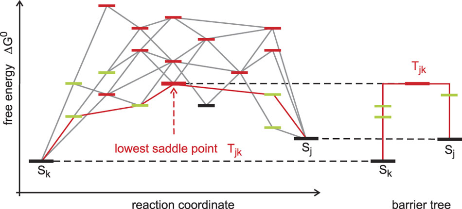
Figure 14 Conformation space and barrier tree. RNA secondary structures formed by one sequence fall into three classes: (i) local minima of the energy surface (black) are surrounded exclusively by suboptimal structures with higher free energies; (ii) saddle points (red) have two (or more) nearest neighbors in shape space that belong to two distinct basins; and (iii) (fully) unstable structures that are neither local minima or saddle points (green). The reaction coordinate is a path in shape space, which leads from one local minimum (conformation S_k) to another local minimum (conformation S_j). The barrier treeReference Flamm, Fontana, Hofacker and Schuster^71, Reference Flamm, Hofacker, Stadler and Wolfinger¹²⁶ is constructed by discarding all structures except local minima of the free energy surface and the lowest saddle points connecting them (an example is shown in Figure 13)

The barrier tree is a coarse-grained simplification of the free energy surface of an RNA molecule. It discards all (fully) unstable structures and retains only (meta)stable conformations and saddle points. The barrier tree, nevertheless, allows for an identification of the basins of attraction (see the example shown in Figure 13). Small basins of attraction can be united to form larger ones until we end up with a few major conformations each defining a large basin, and this procedure can be continued until only very few basins are retained or a single conformation remains. RNA molecules with several dominant basins of attraction corresponding to two or more (meta)stable conformations are called riboswitches, can be designed in silico Reference Flamm, Hofacker, Maurer-Stroh, Stadler and Zehl¹²³ and occur also in vivo.Reference Montange and Batey¹²⁴ Conformational changes in natural riboswitches are commonly triggered by binding of small molecules and have regulatory function in metabolism. The barrier tree has also been used to compute Arrhenius-type folding kinetics of RNA molecules. The results are in good agreement with the exact computations of the folding kinetics on the computed conformational energy landscape unless there are many transition states whose energies lie close by.Reference Wolfinger, Svrcek-Seiler, Flamm, Hofacker and Stadler⁷²

Finally, RNA suboptimal structures can also be considered in the context of sequence-structure mappings.Reference Schuster⁷⁹ The set of structures that are compatible with a given sequence, C(X) considered in Figure 15, is in a way inverse to the set of compatible sequences (C(S) shown in Figure 10) since it deals with a non-invertible mapping in the opposite direction, from shape space into sequence space. A subset of the compatible structures,, which contains all local minima of the free energy surface and the saddle points connecting the basins corresponding to (meta)stable conformations, provides the basis for the construction of barrier trees. All structures that are neither local minima nor saddle points are neglected. Local minima with positive free energies relative to the open chain, ΔG > 0, and saddle points leading into their basins are also excluded. RNA evolution on neutral networks considered as a process with structure conservation and likewise kinetic RNA folding in conformation space is a process with conservation of sequence.Reference Schuster⁷⁹

Figure 15 Suboptimal and compatible structures. Metastable conformations S_k(X) of sequence X are defined by two conditions: (i) ΔG < 0 for folding and (ii) conformation S_k(X) is a local minimum of the free energy surface. These conformations form the set G(X) in shape space. This set is embedded in the set of all structures that are compatible with sequence X,. This compatible set C(X) contains all structures of shape space that are compatible with sequence X. For the consideration of kinetic folding it is useful to include the set of saddle point structures in the set of metastable structures forming thereby the set of structures of sequence X that is needed for the construction of barrier trees: