


Introduction
Landscape evolution in orogenic belts has attracted considerable attention in the earth-sciences community (e.g. Reference KoonsKoons, 1989; Reference Beaumont, Fullsack, Hamilton and McClayBeaumont and others, 1992). New dating methods, such as fission-track analysis (Reference Brown, Summerfield, Gleadow and KirbyBrown and others, 1994) or the determination of exposure ages by cosmogenic isotopes (Reference Nishiizumi, Lal, Klein, Middleton and ArnoldNishiizumi and others, 1986), have provided greater insight into the efficiency of surface processes in shaping a tectonically active area.
At the same time, the increasing power of modern computers has allowed the development of sophisticated surface- processes models in which the evolution of the landscape is commonly assumed to be governed by two types of processes: large-scale fluvial transport and/or local hill-slope diffusion (Reference Willgoose, Bras and Rodriguez-IturbeWillgoose and others, 1991; Reference Beaumont, Fullsack, Hamilton and McClayBeaumont and others, 1992; Reference ChaseChase, 1992; Reference Howard, Dietriech and SeidHoward and others, 1994; Reference Kooi and BeaumontKooi and Beaumont, 1994; Reference Tucker and SlingerlandTucker and Slingerland, 1994). Several studies have investigated the combined effect of both processes on the evolution of rifted margin escarpments (Reference Kooi and BeaumontKooi and Beaumont, 1994; Reference Tucker and SlingerlandTucker and Slingerland, 1994) and zones of continental convergence (Reference Beaumont, Fullsack, Hamilton and McClayBeaumont and others, 1992). Because these models simulate the evolution of the Earth’s surface over longer times and greater distances than are readily observable, the field of computational geomorphology has been plagued by a lack of constraints on the numerous parameters that enter the various model equations. Only limited attempts have been made at constraining these parameters (Reference Van der Beek and BraunVan der Beek and Braun, 1999).
Moreover, the temperate climatic conditions prevailing today in many active orogenic belts (such as the European Alps or the Southern Alps in New Zealand) under which fluvial erosion is dominant, have only existed for a relatively short time. For much of the last two million years, these high elevation, temperate mountain belts have, in fact, been heavily glaciated. In the present study, we wish to investigate the importance of glacial conditions in determining landscape evolution in orogenic belts.
The glacial-erosion model we have developed, like many other geomorphic models, is weakened because several parameters have to be introduced that are difficult to constrain from direct observation and/or experimentation. It is for this reason that we focus on comparing the relative efficiencies of fluvial and glacial erosion and the interplay between the two processes during times of alternating glacial and interglacial periods, rather than on absolute erosion rates.
In this paper, we present a description of the model including the assumptions it is based on, as well as its most interesting predictions. We emphasize that we have not attempted to include all forms of glacial erosion, but to produce a model which parameterizes the large-scale landscape evolution. If the forms and processes that are observed in nature are reproduced by the model, this does not prove that the assumptions on which the model is based are correct, but rather that they are plausible.
Model Description
Surface-processes model
The landscape is described by a bedrock topography, H (x, y), known at a finite number of nodes distributed on a regular rectangular grid, H i. Landscape evolution is assumed to be controlled by three types of processes: (1) long-range fluvial processes, (2) local hill-slope processes (Reference Kooi and BeaumontKooi and Beaumont, 1994) and (3) glacial erosion.
Fluvial erosion
At each point on the landscape, fluvial erosion is assumed proportional to the difference between the actual sediment load, q s, and the stream carrying capacity, q eq (Reference Kooi and BeaumontKooi and Beaumont, 1994):
where S i and l j are the surface area and stream reach length associated with point i on the landscape, and l e,d is a length scale characterizing the erosion—deposition process {Reference Kooi and BeaumontKooi and Beaumont, 1994). If erosion takes place (δH i/δt > 0), l e represents the length scale over which the sediment load will increase by a factor e. l e is a function of the nature of the bedrock: alluvial surfaces {previously deposited sediments) are characterized by a smaller value of l e than intact bedrock, because they are eroded more easily. We assume that streams cannot transport sediment above their carrying capacity, so a value of l d equal to l i is used where deposition takes place (δH i/δt > 0).
The sediment load is calculated by integrating upstream erosion/deposition. The carrying capacity is expressed as a linear function of local slope, ϕ, and water discharge, q w (Reference Kooi and BeaumontKooi and Beaumont, 1994):
where K r is a constant. Water discharge, q w, is the product of the catchment surface area, A c, and the precipitation rate, v r, and is calculated at every point of the landscape via the so-called CASCADE node-ordering algorithm.
Node ordering
At each point i on the landscape, bedrock elevation is updated at each time-step according to the solution of the fluvial erosion—deposition equation. The sediment load and water discharge are then updated and passed to the lowest of the eight adjacent points or, more exactly, the one of the eight neighbours that defines the steepest slope. This operation is performed in a sequence that guarantees that when the equations are solved at point i all upstream properties, such as water discharge and sediment load, have been previously estimated. The ordering of the nodes in that sequence is based on the CASCADE algorithm, developed by Reference Braun and SambridgeBraun and Sambridge (1997).
In CASCADE, each node is given a parcel of water proportional to the local precipitation (assumed constant in the experiments described here) and the surface area attached to the node, Si. Each node gives its water parcel to its lowest neighbour. At the end of this “passing operation”, any node that is left without water is put on a stack. The passing operation is repeated with the remaining nodes and those that are left without water are put on the stack. This simple operation is repeated as many times as necessary until all the water has reached base level (along the sides of the model), all the nodes have been put on the stack, and the water discharge has been calculated for every node. This algorithm yields an ordering of the nodes (in the stack) that is appropriate to solve the geomorphic fluvial equations described above.
Hill-slope processes
Hill-slope processes are regarded as diffusive processes and are incorporated in the model through a simple, linear diffusion equation (Reference Kooi and BeaumontKooi and Beaumont, 1994; Braun and Sambridge,
where K d is a constant. This simplified parameterization is assumed to include a variety of processes such as weathering, slope wash, mass wasting and soil creep.
Ice model
To calculate glacial erosion, we first need to estimate the extent and thickness of ice covering the landscape for given accumulation and ablation rates. To compute the ice thickness, h, we solve the mass-balance equation based on the shallow ice approximation (Reference Knap, Oerlemans and CadeeKnap and others, 1996):
where ![]() is the vertically integrated mass flux (
is the vertically integrated mass flux (![]() where
where ![]() is the vertically integrated horizontal ice velocity) and M is the mass balance which, in our model, includes surface accumulation and basal melting, the two dominant processes that determine net accumulation/ablation in temperate mountain glaciers.
is the vertically integrated horizontal ice velocity) and M is the mass balance which, in our model, includes surface accumulation and basal melting, the two dominant processes that determine net accumulation/ablation in temperate mountain glaciers.
It is clear that the shallow-ice approximation is not appropriate in regions characterized by horizontal gradients in bedrock topography greater than the ice thickness. It is interesting to note, however, that the minimum horizontal- length scale that can be resolved in our computations is given by the grid spacing, Δx = Δy ≈ 2 km, while the maximum ice thickness is of the order of a few hundred meters. Consequently, although the shallow ice approximation may not always be appropriate in high-relief mountainous terrain, it is a relatively sound approximation in our model where, because of its limited spatial resolution, the ratio of ice-thickness to bedrock-topography length scale is of order 1:10.
The ice velocity, ![]() , is the sum of two terms:
, is the sum of two terms:
where ![]() is the deformation velocity and
is the deformation velocity and ![]() is the sliding velocity which may be expressed in the following manner {Reference Knap, Oerlemans and CadeeKnap and others, 1996):
is the sliding velocity which may be expressed in the following manner {Reference Knap, Oerlemans and CadeeKnap and others, 1996):
where α and N define the power-law ice rheology (Reference HookeHooke, 1981):
ρ is the ice density, g is the acceleration due to gravity, A
s is the sliding parameter, N is the ice overburden pressure and P is the water pressure. We shall assume that N — P = 80% N (Reference Knap, Oerlemans and CadeeKnap and others, 1996). This simplification does not take into account the complex spatial variations in basal water pressure observed beneath flowing glaciers {Reference HarborHarbor, 1992). A more rigorous approach would require that the height of the piezometric surface be estimated at every point of the landscape from the flux of water melting at the base of the ice. This is the subject of ongoing work. Note that the sliding velocity, ![]() , is set to zero in regions of the landscape where the ice is frozen to the bedrock {that is where the ice basal temperature is below the melting point) (Reference DrewryDrewry, 1986).
, is set to zero in regions of the landscape where the ice is frozen to the bedrock {that is where the ice basal temperature is below the melting point) (Reference DrewryDrewry, 1986).
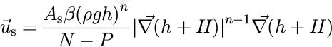
When ice flows down narrow glacial valleys it is well- documented (Svennson, 1959) that the deformation and sliding velocities (and thus basal-shearing stress) are affected by the constriction of ice by the valley walls. We implement this effect by scaling the ice velocities by a “constriction factor”, β, which may be expressed as:
where k c is a constant and δ 2 H/δxf 2 is the second derivative of the bedrock topography in a direction normal to the direction of ice flow.
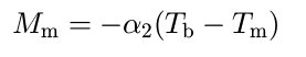
The mass balance term, M, may be regarded as the sum of two terms: M a, the surface accumulation (expressed in m a1), which is assumed proportional to surface temperature, T s (expressed in °C):
where α1 is a constant, and M m, the melting rate at the base, which is assumed proportional to the different between basal temperature, T b, and the melting point, T m = –8.7 × 10⁻⁴ h:
where α is a constant. The ice-surface temperature, T s, is assumed to vary with total elevation and with time, t, through a series of climate cycle of amplitude ΔT 0:
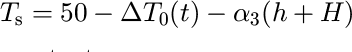
where α3 is constant.
The values of the parameters are chosen to produce a mass-balance-altitude relationship similar to the one proposed by Reference KerrKerr (1993) for areas characterized by a continental climate. The ice basal temperature results from a balance between vertical heat conduction and advection (Reference Siegert and DowdeswellSiegert and Dowdeswell, 1995):
where k is the thermal diffusivity of ice and (δT/δz)b, the imposed basal heat flux.
Glacial-erosion model
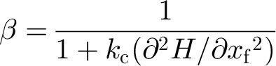
We will adopt Reference HalletHallet”s (1979) hypothesis that glacial erosion is proportional to basal-sliding velocity. Hence, at every point of the landscape where the ice is sliding on the bedrock ![]() glacial erosion is assumed to take place at a rate given by:
glacial erosion is assumed to take place at a rate given by:
where K i is a constant. Following the work of (Reference HarborHarbor, 1992) and for ease of numerical implementation, we shall assume that l — 1. Little constraint is available for the parameter K i; we shall use a value derived from Reference DrewryDrewry (1986; Table 6.1).
Modification to the CASCADE algorithm
We assume that, following local glacial erosion, glacial debris is extracted from the landscape and transported by the ice at the velocity ![]() (the ice velocity). This process can be incorporated in the model by modifying the CASCADE algorithm in the glaciated parts of the landscape in the following ways:
(the ice velocity). This process can be incorporated in the model by modifying the CASCADE algorithm in the glaciated parts of the landscape in the following ways:
-
(1) debris is passed to the one of the eight adjacent nodes that defines the steepest gradient in total ice elevation (this ensures the debris is carried in the direction of ice velocity,
 );
); -
(2) sequencing of the nodes in the CASCADE algorithm is based on the total ice-surface elevation; and
-
(3) at the boundary between glaciated and ice-free parts of the landscape, ice-transported debris is “transformed” into sediment load.
Because the flow of ice on a glaciated landscape is much slower than the flow of water in a river network (Reference DrewryDrewry, 1986), an ice sheet (or mountain glacier) is capable of storing a substantial debris concentration over time-scales of several hundred years. Unlike a fluvial transport model, a glacial transport model must therefore incorporate a storage term. This is incorporated in our model by limiting the amount of debris passed from point i of the landscape to its steepest total ice elevation gradient neighbour by a factor γ determined by the local ice velocity, ![]() , the distance between node i and the node to which the debris is passed, l
i, and the integration time step, Δt:
, the distance between node i and the node to which the debris is passed, l
i, and the integration time step, Δt:
Flexural isostasy
Tectonic deformation within the Earth”s lithosphere leads to surface uplift and mass redistribution at the surface by erosion/deposition. This mass redistribution gives rise to large horizontal gradients in vertical stress that can cause flow in the underlying asthenosphere. On the time and length scales of glacial processes, it is likely that a large proportion of these horizontal stress gradients will be sustained by the lithosphere itself.
To incorporate flexural isostasy in our model, we coupled the surface-processes model to a simple mechanical model representing the behaviour of the lithosphere-asthenosphere system: at each time-step in the model, variations in surface topography are transformed into a load that is applied to a two-dimensional uniform thin elastic plate. The resulting deflection is then incorporated into the tectonic uplift function. Note that this load also includes the mass of the ice.
Parameter Value and Problem Setting
The problem to be solved is that of a relatively fast-growing orogen of small dimension. The equations are solved on a rectangular grid of dimension L x — 100 km x L y — 200 km with a grid spacing of 1.58 km (i.e. 64 × 128 nodes). Model parameter values are given in Table 1. Tectonic activity is represented by an uplift function, u T (x, y), which has the appearance of a rising dome with a Gaussian bell-curve cross-section and defined as:
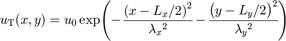
where u 0 — 2 km Myr, λx — 25 km and λy — 50 km.
Table 1. Model parameter values.
A series of glacial cycles is imposed on the model through a time-varying surface-temperature function. Each cycle is 100 kyr long and comprises a short (10 kyr) period of rapid warming followed by a longer (90 kyr) period of cooling. Such a saw-tooth function has been used in previous works (Reference HuybrechtsHuybrechts, 1992, Reference Kerr1996; Reference Pattyn and DecleirPattyn and Decleir, 1995) to simulate the climatic effects of glacial cycles in glacier and ice-sheet models. It is based on the Vostok ice core temperature signal from 150 kyr until present (Reference Pattyn and DecleirPattyn and Decleir, 1995) and on the generally accepted good correlation between high-altitude paleo-air temperatures and indicators of global ice volume (Reference Barrett, Harris and Stone houseBarrett, 1991). The amplitude of the imposed temperature variation is arbitrarily set at ΔT 0 — 2°C.
Model Results
A series of model experiments were performed in which the values of the fluvial erosion constant, K r, and glacial erosion constant, K i, vary while their product remains constant. In doing so, we compare the efficiency of each of the two processes in competition with the other to sculpt a landscape in an orogenic belt characterized by a spatially and temporally “smooth” tectonic uplift function.
It is expected that fluvial processes will be most efficient during periods of low (or no) glaciation, whereas glacial processes will be most efficient during glaciations. The purpose of the modelling is to investigate how each eroding mechanism can adapt to a landscape produced by the other mechanism, and how the landscape evolves through time under these variable conditions.
Experiment I is characterized by intermediate values of the glacial erosion constant and the fluvial erosion constant (K i = K i,0 and K r = K r,0); experiment II is characterized by a low value for the glacial erosion constant (K i = K i,0/2) and a high value for the fluvial erosion constant (K r = K r,0 x 2); experiment III is characterized by a high value for the glacial erosion constant (K i, = K i,0 x 2) and a low value for the fluvial erosion constant (K r = K r,0/2). In experiment IV, no ice is allowed to form; in experiment V, the ice constriction effect is not included (i.e. the factor β in Equations (6) and (7) is set to one). Each experiment is carried out for 520 kyr, which is approximately the length of five glacial cycles.
Results of one model experiment through a glacial cycle
Results from experiment I are illustrated in Figure 1, where the evolution of the bedrock topography and ice thickness throughout the fourth glacial cycle is shown. The landscape is displayed as a three-dimensional surface, illuminated from the top left corner of the image and on which the ice has been draped and coloured in white. The ten panels correspond to 10 kyr intervals from 410 to 500 kyr since the beginning of the experiment.
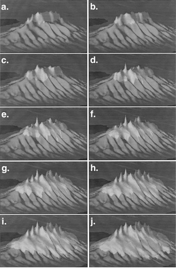
Fig. 1. Results of the computations shown as perspective views of the bedrock topography (dark grey) on which the ice has been draped (light grey). Vertical exaggeration is 40:3. Panels a—j correspond to x 410-500 kyr at 10 kyr intervals.
The bedrock topography is characterized by high-relief mountain tops, deeply incised U-shaped valleys, relatively steep backwalls which make the valleys resemble large cirques, and narrow interfluves. The ice cover is minimum at 410 kyr and grows monotonously from 430 kyr onwards to reach a maximum at the end of the glacial period (i.e. 500 kyr). The distribution of ice is strongly influenced by the underlying bedrock topography: although characterized by the highest accumulation (i.e. precipitation) rates, the peaks are barely glaciated, whereas the valleys forming along the mountain sides host large ice tongues that resemble piedmont glaciers fed by the ice accumulating in the adjacent high-altitude, high-relief regions.
In the following sections, we compare the various experiments in terms of the time evolution of “space-integrated” or “model-averaged” variables such as total ice volume, maximum bedrock topography, glacial and fluvial erosion rates, etc.
Ice volume and topography
Figure 2 shows the evolution of the total volume of ice on the landscape for experiments I to III. The computed ice volume reflects the imposed variations in surface temperature (and hence ice accumulation) and the imposed steady tectonic uplift. During the first glaciation, the elevation of the mountain belt is too low for any ice to accumulate on the landscape. During the following glaciations, ice volume grows almost linearly to reach a maximum at the end of each glaciation (200, 300, 400 and 500 kyr) and then decreases very abruptly within a few thousands years of the glacial maximum. The first two interglacial periods (200— 210 kyr and 300–310 kyr) are ice free, whereas during the last interglacial period (400–410 kyr), some ice is preserved.
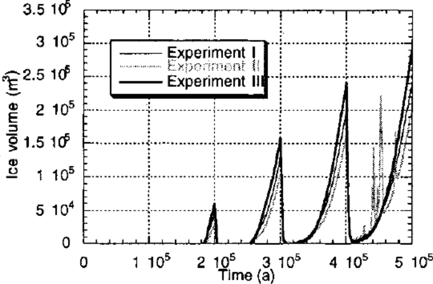
Fig. 2. Computed ice volume as a function of time for experiments I, Hand III.
From these experiments, it is apparent that more ice is formed on a landscape that has been dominantly carved by ice erosion (experiment III) than on a landscape that has been carved by fluvial processes (experiment II). Of the three, experiment III is characterized by the lowest maximum topography (Fig. 3) and, because ice accumulation is proportional to elevation, one might also expect it to have the lowest ice volume. However experiment III actually has the greatest ice volume, demonstrating that it is the form of the landscape that is responsible for differences in “ice retention”, not the absolute value of the topography. This can be further demonstrated by considering Figure 4, where mean bedrock- topography gradient (in the direction of ice flow) is shown as a function of ice thickness for experiments I—III. This diagram clearly shows that landscapes created by glacial processes are, on average, characterized by lower slopes near the ice margins where glacial erosion is most active. It is this reduction in bedrock-topography slope (or the spoon shape of glacial valleys and cirques) near the ice margins that leads to a reduced ice velocity along the edges of the ice sheet and is therefore responsible for the greater ice retention by glacial landscapes.
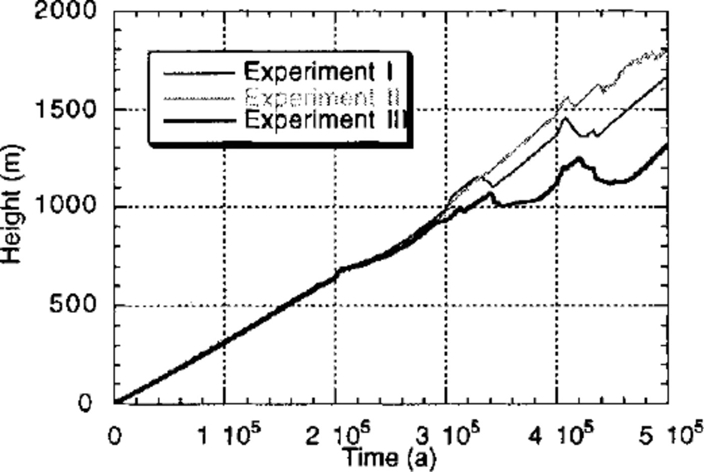
Fig. 3. Computed maximum topography as a function of time for experiments I,II and III. The topography is the result of a balance between tectonic uplift, isostasy and erosion.
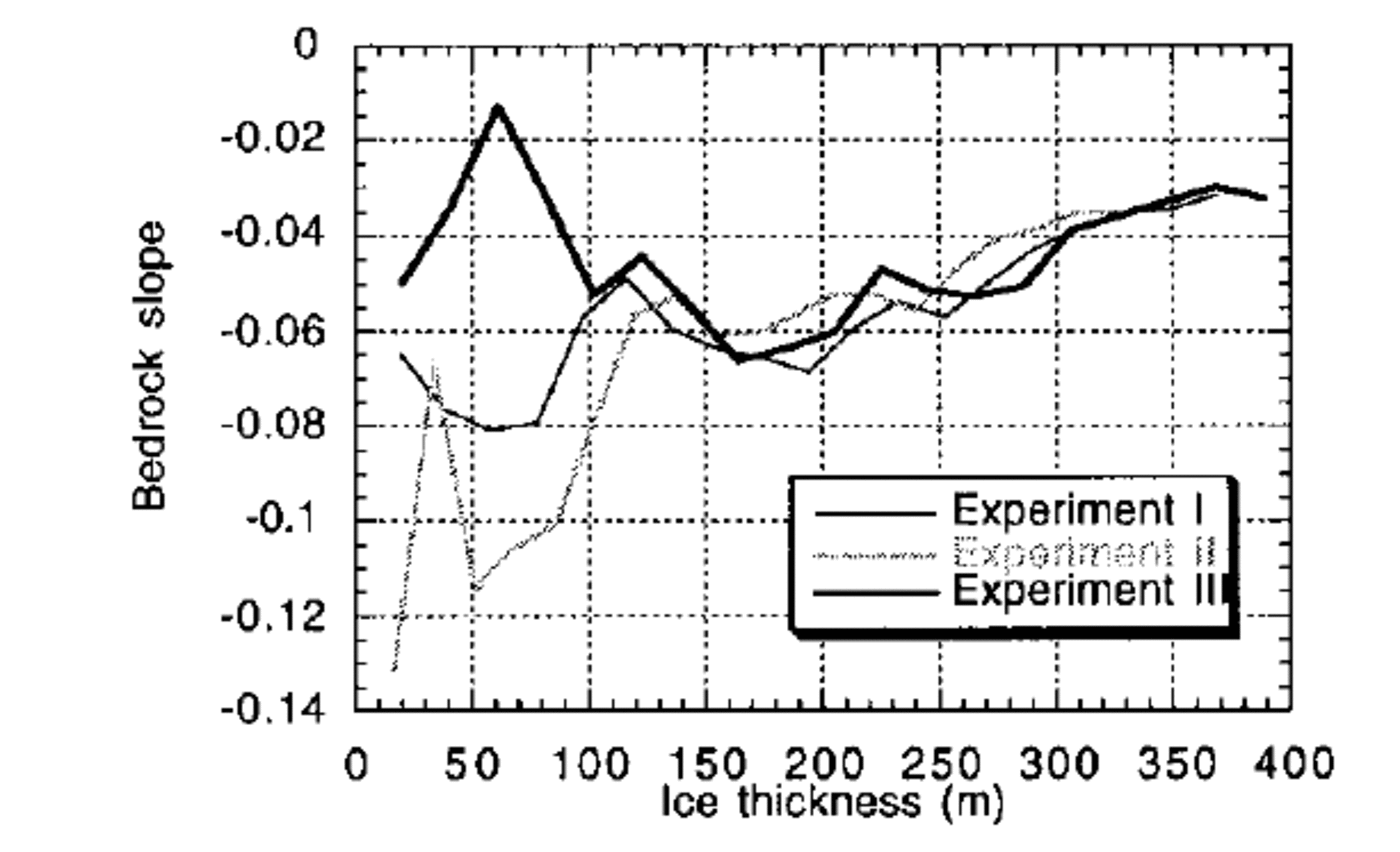
Fig. 4. Mean bedrock slope as a function of ice thickness for experiments I, II and III. Lower slopes near the ice margins indicate the landscape is capable of retaining more ice.
The large, rapid variations in ice volume that charactize the fourth glacial cycle in experiment II (Fig. 2) are of large tongues of ice which develop along the flanks of the further proof of the inability of a fluvial landscape to sustain mountain and render the ice cap unstable. We do not place a large ice cap. These variations correspond to the formation too much significance on the details of the evolution and geometry of these surging instabilities, only to notice they are likely to form in valleys that have recently been carved by a major river along the sides of the mountain. These instabilities are therefore triggered by the grading process that takes place in river valleys during interglacial periods.
Local maxima (drainage divides)
Since the landscape dominated by glacial erosion is characterized by the lowest maximum topography, it suggests glacial erosion is more efficient than fluvial erosion at removing local topographic maxima. It is indeed well known that fluvial processes are, in fact, incapable of eroding material from the summit of drainage divides because these divides are characterized by a zero-area catchment. No such restrictions apply to glacial erosion.
Figure 3 suggests, however, that the glacial erosion of the mountain top is maximum during time of intermediate ice cover. This is because glacial erosion is not possible {1) during the interglacial periods when there is no ice on the mountain top or {2) during the time of maximum glaciation when the ice is frozen to the bedrock at the top of the mountain. This behaviour agrees well with the common observation that large mountain ranges that were covered by continental ice sheets during the last glaciation, such as the Canadian Cordillera (Reference EvansEvans, 1996; Reference Clague and FultonClague, 1989), show little effect of the overriding ice near the summits; most of the evidence for ice abrasion/erosion is found in relatively low-altitude cirques and valleys.
Glacial-erosion rate
In Figure 5, we compare the spatially integrated fluvial and glacial erosion rates calculated from each experiment. As expected, glacial-erosion rate is directly proportional to ice volume. It is nil during ice-free periods and maximum during periods of maximum ice extent. Note, however, that in all experiments the rate of glacial erosion steadily increases from one glacial period to the next, but in experiment III, it remains constant between the last two glaciations. This indicates that, from the third glaciation onwards, despite the fact that the volume of ice is still increasing (see Fig. 2), glacial erosion has reached steady-state.
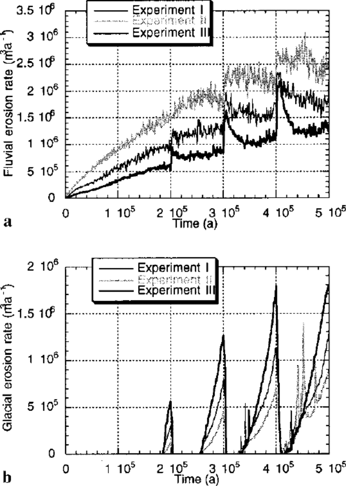
Fig. 5. (a) Computed river erosion rate and (b) glacial erosion rate. These quantities are computed at each time-step by summing the amount of material removed from the landscape by each process and dividing by the time-step length.
To understand this behaviour, one must consider where glacial erosion is taking place beneath the ice. Figure 6a shows a contour plot of the x component of the sliding velocity at the time of the Last Glacial Maximum. This demonstrates that the ice is sliding in the valleys, but is frozen to the bedrock in the regions of high topography {that is the central divide and the major interfluves). Thus, despite the fact that the surface area covered by ice is still increasing from glaciation to glaciation, the surface area covered by sliding ice does not substantially change from the third glaciation onwards.
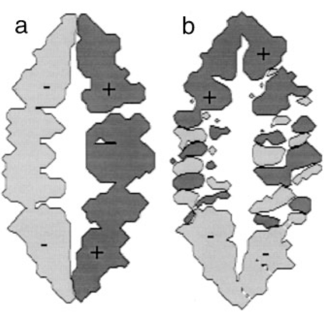
Fig. 6. Computed sliding velocity (a) in the x direction and (b) in the y direction at the end of the last glacial period (500 kyr) in experiment III. The dark-grey regions correspond to positive (eastward and northward) velocities, whereas the light-grey regions correspond to negative velocities (westward and southward). Notice in panel (b) the ice-flow convergence near the top of the glacial valleys (or névés) and the flow divergence in the unconstricted glaciers’ tongues (or piedmont glaciers).
Fluvial-erosion rate
Overall, the fluvial erosion rate increases with time in all three experiments. In the second experiment, the fluvial erosion rate decreases during glacial periods; whereas in the third experiment, the fluvial erosion rate increases during interglacial periods. The first experiment displays an intermediate behaviour. The reduction in fluvial erosion rate during glacial periods is directly related to the presence of ice that prevents fluvial incision and transport from operating.
The increase in fluvial erosion rate during interglacial periods is caused by the imbalance between the form of the glaciated landscape and the process of river incision. At the end of a glacial period, the landscape includes formerly glaciated valleys that are characterized by a steep backwall and a relatively flat valley floor (see Fig. 7). Some of the valleys are, in fact, filled by lakes, as they are terminated by a raised sill which formed along the margin of the ice cap. When such a landscape is suddenly freed of ice and river incision is allowed to take place, rapid incision of the flat river beds and sills takes place leading to a pulse in fluvial erosion rate by “glacial nickpoint retreat”. The removal, by the fluvial network, of relatively soft glacial debris deposited during glacial retreat also contributes to the increased fluvial erosion rate immediately after a glaciation.
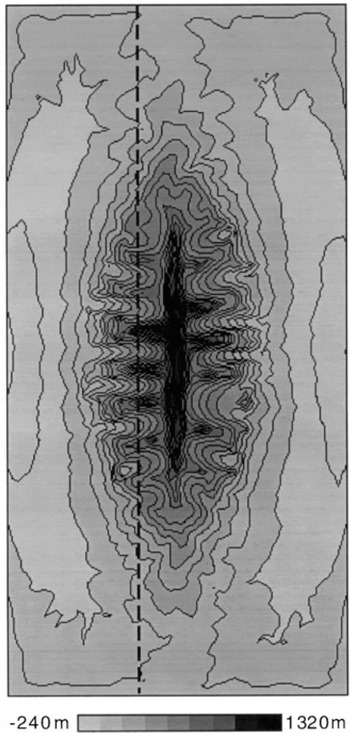
Fig. 7. Computed topography at the end of the last glacial period (500 kyr) in experiment III. White to light-grey areas correspond to low topography; dark-grey to black areas correspond to high topography.
Large mass movements by fluvial erosion/transport have been documented in many mountainous areas following deglaciation. A spectacular example of such processes took place at the end of the last glaciation in the Lahul Himalaya, northern India (Reference OwenOwen and others, 1995), where paraglacial reworking of unconsolidated glaciogenic sediments and rapid degradation of glacial landforms by fluvial processes led to the release of large quantities of sediments into the present-day fluvial system. A similar readjustment of the landscape has also been observed around retreating glaciers in Norway (see, e.g., Reference Ballantyne and BennBallantyne and Benn, 1994).
Drainage patterns
Another important contribution to the imbalance between fluvial and glacial erosion processes comes from the difference between ice and water flow along the sides of a mountain. Water flows downhill, that is by following the local topographic gradient, whereas ice flows in the direction of steepest ice-surface gradient. Although on average the two directions coincide, locally they may diverge substantially. This is illustrated in Figure 6b, where a contour map of the y component of the ice-sliding velocity is shown. In the “northern”” part of the mountain belt, there is a finite northward component to the sliding velocity in east—west trending valleys; conversely, in the southern part of the mountain belt, there is a finite southward component in east—west trending valleys. Valleys in the northern and southern parts of the mountain belt, that have experienced ice flow in a direction oblique to the local topographic gradient, are wider than the valleys in the central parts of the mountain belt (Fig. 7).
This difference between ice and water-drainage patterns can be measured by the proportion of the nodes discretizing the landscape where the direction of ice flow is different from the direction of water flow. This proportion reaches 12% at the peak of the last glaciation in experiment III.
Ice constriction
Valley cross-sections are shown in Figure 8a, along a north— south profile that runs along the side of the mountain belt 10 km to the west of the main drainage divide. The geometry of the valleys at the peak of the Last Glacial Maximum in experiment III are U-shaped and separated by very “sharp” interfluves (inverted Vs). This geometry contrasts with that of experiment IV, in which no ice is allowed to develop on the landscape (Fig. 8b). In this case, the valleys are V- shaped and the interfluves are rounded (inverted Us).
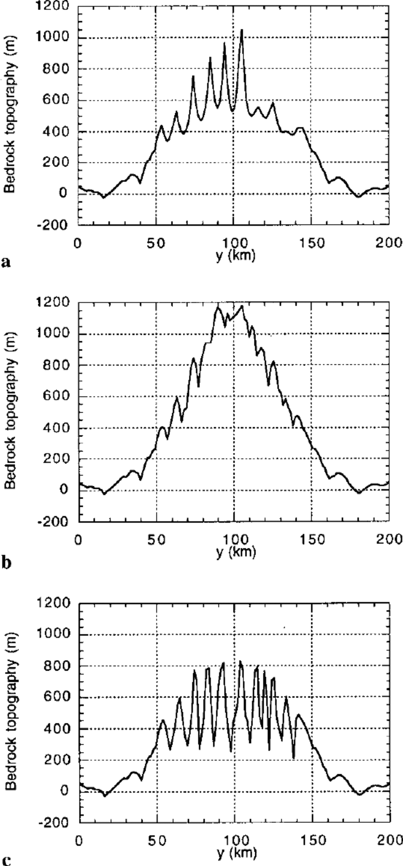
Fig. 8. Topographic cross-sections computed along a north- south line shown on Figure 7 for experiments (a) III, (b) IV and (c) Vat t = 500 kyr.
The characteristic U-shape of the glacial valleys is imposed in our model by the ice-constriction factor, β. This is clearly demonstrated by the results of experiment V, identical to experiment III but for the constriction parameter, kc , which is set to zero (leading to β — 1 everywhere). The resulting valley cross-sections are V-shaped (Fig. 8c). Note, however, that in this fifth experiment the downstream profiles of the glacial valleys were identical to those of experiment III leading to the formation of narrow, spoonshaped, glacial lakes. In experiment V, the pulses in fluvial erosion rate following the glacial periods are of greater magnitude and the ice volume supported by the landscape is larger than in experiment III. This demonstrates that the imbalance between glaciated and fluvial landscapes predicted by our model does not come from the imposed ice- constriction term which we arbitrarily included in the model and which strongly dictates the cross-sectional shape of glacial/fluvial valleys. Rather, this imbalance is a more fundamental consequence of the basic difference between glacial and fluvial erosion processes which create their own characteristic landforms in the direction of ice/water movement: glacial cirques/lakes versus graded river profiles.
Conclusions
Glacial landscapes have a form that is better suited to hold large ice volumes than fluvial landscapes;
unlike water streams, glaciers are capable of eroding drainage divides, but only for moderate ice thickness under the conditions modelled here;
glacial erosion may rapidly reach a constant rate even in a steadily growing orogen; therefore, ice erosion cannot keep pace with tectonic uplift once a critical topography is reached;
disequilibrium between fluvial and glacial landforms leads to large pulses in erosion rate {and thus, sediment flux) at the end of glacial periods; and
this disequilibrium comes from the spoon-like shape of glacial valleys and lakes which are eroded away by rapid nick-point retreat at the end of glacial periods; the disequilibrium also results from the difference in local drainage patterns between the fluvial network and the ice-sheet flow.
Our model is based on a collection of relatively well-established concepts concerning fluvial and ice erosion; it is therefore not surprising that it predicts behaviours that are also relatively well understood. Its originality comes from its ability to combine, in space and time, processes that have usually been studied separately in the past. Work is under way to further improve this geomorphic model and to compare its predictions to natural examples.
Acknowledgements
The authors wish to thank A. Kerr and J. M. Harbor for very constructive comments made on a previous version of this manuscript.


