


Implications
Costs of genomic selection breeding scheme are especially important, when the goal is to improve a novel trait, such as methane emission or feed intake, where reliable phenotyping is expensive. Creating reference population providing high genomic breeding values reliability is challenging. Another challenge is maintaining reference population such that initially achieved reliability does not drop. This study investigated minimum number of cows to be used for updating reference population to keep reliability constant at initially achieved level. Presented approach provides insights in designs of optimal strategies to keep reference population up-to-date across several generations in the population under selection pressure.
Introduction
High reliability of estimated breeding values is important for achieving high genetic progress – a key feature of a successful breeding programme. Introducing genomic selection (GS) (Meuwissen et al., Reference Meuwissen, Hayes and Goddard2001) into the breeding practice enabled an increase in the reliability of breeding values for animals without offspring performance (Sellner et al., 2007; Hayes et al., Reference Hayes, Bowman, Chamberlain and Goddard2009; Calus, Reference Calus2010) which is especially important for dairy cattle breeding. As the animals can be accurately selected at young age, GS enables to accelerate the generation turnover and thus to reduce the generation interval (for reviews see: Pryce and Daetwyler, Reference Pryce and Daetwyler2012; Bouquet and Juga, Reference Bouquet and Juga2013).
A reference population (RP) is a key element of GS. The RP consists of genotyped animals with phenotypic observations either based on own or progeny performance. The RP is used to predict the single nucleotide polymorphism (SNP) effects which are then used to estimate the genomic breeding values (DGV) of selection candidates. One of the most important features of the RP influencing the DGV reliability is its size. A larger RP generally results in a higher DGV reliability (Goddard and Hayes, Reference Goddard and Hayes2009; Hayes et al., Reference Hayes, Bowman, Chamberlain and Goddard2009). Another important aspect is the RP design. An optimally designed RP is expected to maximize the reliability for a given population (Pszczola et al., Reference Pszczola, Strabel, Mulder and Calus2012a; Rincent et al., Reference Rincent, Laloë, Nicolas, Altmann, Brunel, Revilla, RodrĂguez, Moreno-Gonzalez, Melchinger, Bauer, Schoen, Meyer, Giauffret, Bauland, Jamin, Laborde, Monod, Flament, Charcosset and Moreau2012; Isidro et al., Reference Isidro, Jannink, Akdemir, Poland, Heslot and Sorrells2015). Several studies have shown that across scenarios the highest accuracies were obtained when the RP consisted of animals that are distantly related to each other (Clark et al., Reference Clark, Hickey, Daetwyler and van der Werf2012; Pszczola et al., Reference Pszczola, Strabel, Mulder and Calus2012a; Rincent et al., Reference Rincent, Laloë, Nicolas, Altmann, Brunel, Revilla, RodrĂguez, Moreno-Gonzalez, Melchinger, Bauer, Schoen, Meyer, Giauffret, Bauland, Jamin, Laborde, Monod, Flament, Charcosset and Moreau2012; Isidro et al., Reference Isidro, Jannink, Akdemir, Poland, Heslot and Sorrells2015; Wu et al., Reference Wu, Lund, Sun, Zhang and Su2015) and closely related to the evaluated animals (EVA) (Habier et al., Reference Habier, Tetens, Seefried, Lichtner and Thaller2010; Pszczola et al., Reference Pszczola, Strabel, Mulder and Calus2012a; Wu et al., Reference Wu, Lund, Sun, Zhang and Su2015).
The DGV reliability decays over generations if RP is not updated (Meuwissen et al., Reference Meuwissen, Hayes and Goddard2001; Calus, Reference Calus2010; Wolc et al., Reference Wolc, Arango, Settar, Fulton, O’Sullivan, Preisinger, Habier, Fernando, Garrick and Dekkers2011), because the relationships between the EVA and the RP drop (Habier et al., Reference Habier, Fernando and Dekkers2007; Wolc et al., Reference Wolc, Arango, Settar, Fulton, O’Sullivan, Preisinger, Habier, Fernando, Garrick and Dekkers2011; Pszczola et al., Reference Pszczola, Strabel, Mulder and Calus2012a). Another explanation for such decline in the DGV reliability is the decay in linkage-disequilibrium (LD) between SNPs and quantitative trait loci (QTL) over generations. Consequently, it is important to update the RP with animals from the new generations to maintain the reliability constant at its initial level.
Updating the RP may sometimes be challenging either because of the genotyping costs or difficulties in obtaining reliable phenotypes. To minimize costs of running a GS-based breeding programme, an important question is what is the minimum size of the RP update in order to keep the reliability at a constant level. Therefore, the objective of this study was to investigate how many animals per generation are needed to be added to the RP to keep the reliability at a constant level across generations. This minimum RP update size is specifically investigated for a scenario with a novel trait for which only an initially small cow RP (n=2000) with own phenotypes is available, and where additional cows are added every generation. Examples of such a trait are methane emission or feed intake in dairy cattle. In this study, we assumed that the update of the RP uses phenotypes with the same accuracy measured on the same category of animals. In practical implementations these assumptions might need to be adapted for novel traits for which initial accurate RP phenotypes are available only for a limited number of animals and only less accurate phenotyping may be done during the updating process. For example, when the update could be done using indirect measurements of the novel trait (e.g. mid-IR spectra prediction of methane emission from milk).
Material and methods
Data
To assess the minimum RP update size, we have simulated a dairy cattle population with phenotypes recorded for a novel trait. In the simulation process, the history of cattle breeding was simulated using QMSim software (Sargolzaei and Schenkel, Reference Sargolzaei and Schenkel2009). The values of the effective population size (N e ) reflected different points in the history of the US and Canadian Holstein cattle (Schenkel et al., Reference Schenkel, Sargolzaei, Kistemaker, Jansen, Sullivan, Van Doormaal, VanRaden and Wiggans2009).
Historic population
In total, 505 historical generations were simulated. The number of animals (n) at 500, 250 generations ago and in five generations ago were assumed to be ~1400, 1000 and 100, respectively. This decline in N across generations was applied to achieve a level of N e in the final generations that is similar to the N e in the current Holstein population. The animals in the historic populations were mated randomly and the sex ratio was assumed to be 0.5. The simulated genome consisted of 29 autosomes with a total genome length of 2333cM. Chromosomes were given the same length as observed in cattle data by Snelling et al. (Reference Snelling, Chiu, Schein, Hobbs, Abbey, Adelson, Aerts, Bennett, Bosdet, Boussaha, Brauning, Caetano, Costa, Crawford, Dalrymple, Eggen, Everts-van der Wind, Floriot, Gautier, Gill, Green, Holt, Jann, Jones, Kappes, Keele, de Jong, Larkin, Lewin and McEwan2007). Initially, 46660 markers and 7250 QTL were evenly spaced across the genome with equal allele frequencies for both alleles. Mutation rate for markers and QTL was 2.5×10⁻⁵. The first generation consisted of 1400 individuals. The number of animals was reduced linearly in the subsequent generations until after 250 generations it reached 1000 individuals. In the next 250 generations the number of the animals was reduced until it reached 100 individuals. The first part of the simulation resembled the bottleneck present in the history of cattle breeding and enabled to reach the LD level which was realistic for the current Holstein dairy cattle population. In the last five generation of the historic population the number of females was increased to 5000 and the number of males was set to 25.
Current population
All the animals from the last generation of the historic population were considered to be the founders of the modern population. Each of 25 males per generation was mated randomly with 5000 females. Each female produced one offspring which had a 50% chance of being male or female. The replacement ratio for females was 0.5 resulting in overlapping generations. The age of the animals was assumed to be the only reason of culling. The mating scheme included selection of males, while there was no selection among females. Selection was based on estimated breeding values for an overall index trait (as explained in more detail later), which were approximated with an assumed accuracy of 0.95, which reflects a progeny testing scheme with 150 progeny with one record each per sire for a trait with a heritability of 0.25. Each generation, the 25 males with highest breeding values were chosen to sire the next generation. The first 10 generations of selection were used to establish Bulmer equilibrium. The 11th generation of the simulation scheme was assumed to be the initial generation for further analysis and will be called generation 0 (Gen0) hereafter. Another five generations (Gen1 to Gen5) were simulated to create a dataset for analyses. In those final generations, 43256 segregating markers and 6734 QTL remained. The whole simulation process was replicated 10 times.
Phenotypes
Our aim was to mimic a novel trait which is currently not included in the breeding goal but it is genetically correlated with it. Therefore, we simulated two genetically correlated traits. The first trait resembled a breeding goal trait under selection pressure and was simulated using the QMSim software. The assumed heritability of this trait was 0.25. The second trait mimicking the novel trait was simulated using the output from QMSim. The procedure for simulating the phenotypes and true breeding values (TBVs) for the second trait was the following:
-
1. The QTL effects for the breeding objective (trait 1), as obtained from QMSim, were standardized to follow a normal distribution N(0,1).
-
2. Half of the QTL effects for the novel trait were drawn randomly from a normal distribution N(0,1), that is independent of the breeding objective trait.
-
3. The other half of QTL effects for the novel trait were drawn from a multivariate distribution, considering the known QTL effects for the breeding objective as obtained from QMSim and a correlation between the QTL effects of both traits of 0.5 (using a Cholesky decomposition of the corresponding co-variance matrix).
-
4. TBVs were obtained by summing all the QTL effects for the novel trait.
-
5. Phenotypes were calculated by drawing a random residual terms from the normal distribution N(0,σ 2 e), where σ 2 e reflected the heritability of 0.2.
The above procedure resulted in phenotypes for the novel trait with a genetic correlation of 0.25 with the index trait (under the assumption that the residual correlation is zero), meaning that selection for an increase in the index trait will indirectly lead to an improvement of the novel trait.
Only the second trait was used in further analyses.
RP and EVA
RP and EVA were sampled randomly from the 2500 females available per generation. The initial RP consisted of 2000 females from Gen0. A total of 500 EVA/generation were sampled randomly from Gen0 to Gen5 and the remaining 2000 females in each generation were considered to be available for possible RP updates.
Breeding values estimation
The initial RP of 2000 cows was used to estimate variance components. The following animal model was fitted using ASReml 3.0 (Gilmour et al., Reference Gilmour, Gogel, Cullis and Thompson2009):
 $$y_{j} ={\equals}\mu {\plus}animal_{j} {\plus}e_{j} $$
where y j is the phenotypic record of animal j, μ j the overall mean, animal j the (random) DGV of animal j and e j a random residual term. In the analyses we used the genomic relationship matrix (G) created with the first formula described by VanRaden (Reference VanRaden2008) using allele frequencies computed across the 2000 initial RP. The variance components were estimated using the initial RP and then used to estimate DGV in the following BLUP analyses using model (1) fitted in ASReml 3.0 (Gilmour et al., Reference Gilmour, Gogel, Cullis and Thompson2009).
Reliability
The reliability was calculated as the squared correlation of the DGV estimated for the EVA and their simulated TBVs. The initial reliability was computed, within each replicate, as the DGV reliability for the EVA from Gen0. All the other reliabilities were calculated for EVA one generation younger than the current RP (e.g. EVA from Gen1 were used to compute the reliability for the RP from Gen0).
RP update
The initial RP was updated by adding batches of 100 animals until the current reliability was equal to or higher than the initial reliability. The added animals originated from the same generation as the current EVA. This resembles a scenario where contemporaries of the selection candidates are genotyped and phenotyped for the novel trait. In practical terms, it may for instance reflect a scenario where measuring the novel phenotype on the EVA is prohibitive. Examples are traits for which phenotyping is too expensive to perform for all EVA, involves a challenge test such as for disease traits, or where the phenotyping should be performed under field conditions while the selection candidates are kept in a nucleus environment. Because the relationship between RP and EVA was shown previously to have an impact on the DGV reliability (Pszczola et al., Reference Pszczola, Strabel, Mulder and Calus2012a), the animals for the RP update were sorted according to their relationship with EVA and first the most closely related animals were added. This relationship was measured as the sum of squared relationship between potential RP update and current EVA. After reaching the initial reliability the EVA from the next generation was evaluated using the updated RP. Further, the update animals were from the same generation as the EVA. In this way, the size of the updated RP was increasing depending on the number of updates required to re-gain the initial reliability. To compare the impact of the updating procedure on the reliability, we also performed genomic evaluation in the five consecutive generations without updating RP.
Indicators for the reliability
Reliability of DGV can be predicted using a selection index-based formula, which utilize relationships between RP and EVA and the relationships within RP (VanRaden, Reference VanRaden2008; Pszczola et al., Reference Pszczola, Strabel, Mulder and Calus2012a). Note that the formulas presented by Pszczola et al. (Reference Pszczola, Strabel, Mulder and Calus2012a) and Goddard et al. (2011) account for sampling errors in the G matrix, while the formula of VanRaden (Reference VanRaden2008) does not. From the formulas presented by VanRaden (Reference VanRaden2008) and Pszczola et al. (Reference Pszczola, Strabel, Mulder and Calus2012a) it can be easily derived that the sum of squared relationships between RP and EVA and the inverse of the genomic relationship matrix of the RP affects the reliability. High relationships between RP and EVA lead to an increase in the reliability. However, high relationships between the animals in RP, are expected to lead to high negative values in the inverse of G, potentially reducing the reliability. Therefore, both squared relationships between RP and EVA and the elements in G −1 for the RP could be potentially used to predict the reliability. It is worthwhile noting that the impact of diagonal and off-diagonal elements in G −1 for the RP may differ. We tested the predictive ability of these parameters for the obtained reliability in regression analyses. First, following single regression analyses were performed:
 $$y_{i} ={\equals}\beta _{0} {\plus}\beta _{1} x_{1} $$
where y
i
was the DGV reliability for the update round i, that is every added batch of 100 reference animals, β
0 the intercept and β
1 the regression coefficients and x
1 an independent variable. In the first model (Reg1) x
1 was the sum of squared relationships between RP and EVA ( $\mathop{\sum}{{\bf{G}} _{{RP,EVA}}^{2} } $
), in the second model (Reg2), x
1 was the sum of off-diagonals of G
−1
for RP (
$\mathop{\sum}{{\bf{G}} _{{RP,EVA}}^{2} } $
), in the second model (Reg2), x
1 was the sum of off-diagonals of G
−1
for RP ( $\mathop{\sum}{{\bf{G}} _{{RP_{{12,21}} }}^{{{\minus}1}} } $
), and in (Reg3), x
1 was the sum of elements of G
−1
for RP (
$\mathop{\sum}{{\bf{G}} _{{RP_{{12,21}} }}^{{{\minus}1}} } $
), and in (Reg3), x
1 was the sum of elements of G
−1
for RP ( $\mathop{\sum}{{\bf{G}} _{{RP}}^{{{\minus}1}} } $
). In addition, we tested if the sum of the off-diagonals of the non-inverted relationship matrix G (
$\mathop{\sum}{{\bf{G}} _{{RP}}^{{{\minus}1}} } $
). In addition, we tested if the sum of the off-diagonals of the non-inverted relationship matrix G ( $\mathop{\sum}{{\bf{G}} _{{RP_{{12,21}} }}^{{}} } $
) was a good predictor of the reliability as this would save the need to invert G (Reg4). Then the best predictor of Reg2, Reg3 and Reg4 was combined with the predictor of Reg1 (i.e.
$\mathop{\sum}{{\bf{G}} _{{RP_{{12,21}} }}^{{}} } $
) was a good predictor of the reliability as this would save the need to invert G (Reg4). Then the best predictor of Reg2, Reg3 and Reg4 was combined with the predictor of Reg1 (i.e. $\mathop{\sum}{{\bf{G}} _{{RP,EVA}}^{2} } {\plus}\mathop{\sum}{{\bf{G}} _{{RP_{{12,21}} }}^{{{\minus}1}} } $
) in a multiple regression model (MultiReg) as follows:
$\mathop{\sum}{{\bf{G}} _{{RP,EVA}}^{2} } {\plus}\mathop{\sum}{{\bf{G}} _{{RP_{{12,21}} }}^{{{\minus}1}} } $
) in a multiple regression model (MultiReg) as follows:
 $$y_{i} ={\equals}\beta _{0} {\plus}\beta _{1} x_{1} {\plus}\beta _{2} x_{2} $$
where y i was the within replicate DGV reliability for the update round i; β 0 the intercept and β 1, β 2 the regression coefficients and x 1, x 2 the independent variables.
Results and discussion
The objective of this study was to investigate the required size of RP update per generation for a novel trait when using the same type of animals with the goal to keep the reliability at a constant level across generations. The considered novel trait mimics a trait for which the number of phenotypes is a limiting factor (e.g. methane emission, feed intake). Such novel traits are usually not yet included in the breeding objectives. Nonetheless, they may indirectly be affected by selection through the genetic correlations with the traits in the breeding objective. To reflect such a scenario, we performed simulations in which the selection pressure was put on the index trait and affected the novel trait only indirectly. This resembles a situation in which for example direct selection on milk yield indirectly improves feed efficiency (Veerkamp, Reference Veerkamp1998) or reduces methane intensity (i.e. methane emitted per kilogram of milk) from the cows (Bell et al., Reference Bell, Wall, Russell, Morgan and Simm2010; Wall et al., Reference Wall, Simm and Moran2010). The animals used to update RP were chosen from the same generation as the evaluated individuals. Such a scenario is likely when creating and updating RP for the novel traits for which recording was initialized in recent times and no historical information is available.
Reliability
The average initial reliability was 0.37 (SE 0.01) and within five generations of GS with no RP update it dropped to 0.21 (SE 0.02) as shown in Figure 1. The reliability appears to decay asymptotically towards a baseline. Closer inspection of rates of decay in real data could confirm this pattern giving more insight into reasons of decay pattern. The presented results showed a clear drop in DGV reliability across generations when the RP is not updated, as noted previously in other studies as well (Sonesson and Meuwissen, Reference Sonesson and Meuwissen2009; Habier et al., Reference Habier, Tetens, Seefried, Lichtner and Thaller2010; Wolc et al., Reference Wolc, Arango, Settar, Fulton, O’Sullivan, Preisinger, Habier, Fernando, Garrick and Dekkers2011; Pszczola et al., Reference Pszczola, Strabel, Mulder and Calus2012a and Reference Pszczola, Strabel, van Arendonk and Calus2012b). Similarly to the results reported by these authors the largest drop in reliability was observed after the first generation. In the present study, without updating RP, the DGV reliability after the first generation of selection on average dropped by 0.08 to drop by a further 0.08 across the remaining four generations. Updating the RP, as expected, enabled to maintain the DGV reliability across generations at the initial value.

Figure 1 Reliability of genomic breeding values across generations without updating the reference population (dashed line) and with update (solid line).
The average update size required to at least re-gain the initial reliability was 576 animals/generation and varied considerably across replicates as shown by the SE of 79. This indicates that other factors than the number of the animals in RP, such as the relationship between RP and EVA animals that may vary across generations and replicates, also plays an important role in determining the update size. In addition, in this study a particular population structure was simulated, in case of a different population structure the number of the updates needed might be somewhat different to the one presented here.
Indicators for DGV reliability
To investigate the impact of the RP design the relationships between animals within RP and between RP and EVA were evaluated. The regression analyses showed a variation in the percentage of variance in the reliability explained by the applied regression models (Table 1). Reg1 which included only sum of squared relationships between RP and EVA explained 31% of the variation whereas the models that utilized relationships within the RP explained from 24% to 34% of the variance. The models using sum of the off-diagonals of the G or sum of the off-diagonals of the G −1 showed similar predictive power (R 2=0.32 and 0.34) whereas the model using the full matrix was inferior (R 2=0.24). The slopes in Reg1 were expected to be positive, as higher relationships between RP and EVA lead a higher reliability (Habier et al., Reference Habier, Tetens, Seefried, Lichtner and Thaller2010; Clark et al., Reference Clark, Hickey, Daetwyler and van der Werf2012; Pszczola et al., Reference Pszczola, Strabel, Mulder and Calus2012a; Rincent et al., Reference Rincent, Laloë, Nicolas, Altmann, Brunel, Revilla, RodrĂguez, Moreno-Gonzalez, Melchinger, Bauer, Schoen, Meyer, Giauffret, Bauland, Jamin, Laborde, Monod, Flament, Charcosset and Moreau2012; Isidro et al., Reference Isidro, Jannink, Akdemir, Poland, Heslot and Sorrells2015; Wu et al., Reference Wu, Lund, Sun, Zhang and Su2015). This was confirmed by the results of the current study as shown in Table 1. In addition, low relationships in RP are desired (Pszczola et al., Reference Pszczola, Strabel, Mulder and Calus2012a; Rincent et al., Reference Rincent, Laloë, Nicolas, Altmann, Brunel, Revilla, RodrĂguez, Moreno-Gonzalez, Melchinger, Bauer, Schoen, Meyer, Giauffret, Bauland, Jamin, Laborde, Monod, Flament, Charcosset and Moreau2012; Isidro et al., Reference Isidro, Jannink, Akdemir, Poland, Heslot and Sorrells2015; Wu et al., Reference Wu, Lund, Sun, Zhang and Su2015). Therefore, the slope in Reg2, which uses the off-diagonal elements of the inverted G, is expected to be positive (as confirmed by the results in Table 2). This is because many high positive relationships in G lead to many negative values in the G −1 . The slope in Reg2 was indeed positive as shown in Table 2. The regression coefficient of Reg4 was expected to be negative, because higher relationships within the RP lead to lower reliability, while it turned out to be positive. This unexpected behaviour together with the somewhat lower R 2 value than for Reg2, use of Reg4 is not advisable.
Table 1 R Footnote 2 values of the regression analyses with the reliability of genomic breeding value as dependent variable
The presented results are averaged across 10 replicates of the whole simulation process and accompanied by the between replicates standard errors.
1 ${\bf{G}} _{{RP,EVA}}^{2} $
–squared genomic relationships between reference population and evaluated animals.
${\bf{G}} _{{RP,EVA}}^{2} $
–squared genomic relationships between reference population and evaluated animals.
2 ${\bf{G}} _{{RP_{{12,21}} }}^{{{\minus}1}} $
– off-diagonal elements of inverse of genomic relationship matrix for reference population.
${\bf{G}} _{{RP_{{12,21}} }}^{{{\minus}1}} $
– off-diagonal elements of inverse of genomic relationship matrix for reference population.
3 ${\bf{G}} _{{RP}}^{{{\minus}1}} $
– inverse of genomic relationship matrix for reference population.
${\bf{G}} _{{RP}}^{{{\minus}1}} $
– inverse of genomic relationship matrix for reference population.
Table 2 Regression coefficients form the performed regression analyses
In all the models the dependent variable was reliability of genomic breeding value and independent variables included: Reg1 – genomic relationships between reference population (RP) and evaluated animals ( $\mathop{\sum}{{\bf{G}} _{{RP,EVA}}^{2} } $
); Reg2 – off-diagonal coefficients of genomic relationship matrix for RP-G
RP
(
$\mathop{\sum}{{\bf{G}} _{{RP,EVA}}^{2} } $
); Reg2 – off-diagonal coefficients of genomic relationship matrix for RP-G
RP
( $\mathop{\sum}{{\bf{G}} _{{RP_{{12,21}} }}^{{{\minus}1}} } $
); Reg3 – all elements in G
RP
(
$\mathop{\sum}{{\bf{G}} _{{RP_{{12,21}} }}^{{{\minus}1}} } $
); Reg3 – all elements in G
RP
(
 $$\mathop{\sum}{{\bf{G}} _{{RP}}^{{{\minus}1}} } $$
); Reg4 – off-diagonals of G
RP
$$\mathop{\sum}{{\bf{G}} _{{RP}}^{{{\minus}1}} } $$
); Reg4 – off-diagonals of G
RP $\mathop{\sum}{{\bf{G}} _{{RP_{{12,21}} }}^{{}} } $
; MultiReg – combination of Reg1 and Reg3 (
$\mathop{\sum}{{\bf{G}} _{{RP_{{12,21}} }}^{{}} } $
; MultiReg – combination of Reg1 and Reg3 ( $\mathop{\sum}{{\bf{G}} _{{RP,EVA}}^{2} } {\plus}\mathop{\sum}{{\bf{G}} _{{RP_{{12,21}} }}^{{{\minus}1}} } $
). The presented results are averaged across 10 replicates of the whole simulation process and accompanied by the between replicates standard errors.
$\mathop{\sum}{{\bf{G}} _{{RP,EVA}}^{2} } {\plus}\mathop{\sum}{{\bf{G}} _{{RP_{{12,21}} }}^{{{\minus}1}} } $
). The presented results are averaged across 10 replicates of the whole simulation process and accompanied by the between replicates standard errors.
Based the R 2 of the above single regression analyses Reg1 and Reg2 were combined in the multiple regression model (MultiReg). This resulted in the highest predictive ability of the reliability. The MultiReg model explained 53% of the variance in the reliability which was only 16% less variance in the reliability explained than the sum of the variance explained by the models Reg1 and Reg2. This means that relationships between RP and EVA and relationships within RP explain largely different part of the variation in the reliability, and thus have to be considered jointly. Figure 2 shows DGV reliabilities against sum of squared relationships between RP and EVA for one randomly chosen replicate, indicated clear patterns across generations. These patterns indicate that a part of the unexplained variance in reliabilities by the regression models is perhaps due to differences across generations as a result of selection (i.e. changes in LD between SNP and QTL or in allele frequencies of QTL) that are not accounted for in the formula. Some sort of correction in the regression analyses accounting for (the number of) generations could improve the predictive power of the models.
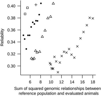
Figure 2 Reliability of genomic breeding values v. sum of squared genomic relationships between reference population and evaluated animals plotted for evaluated animals from generations one to five (indicated, respectively, by the following symbols: □, ●, +, Δ and ×) for one replicate.
Updating strategy
The results of the regression analyses indicate that the optimal updating scheme for the RP considers both relationships between RP and EVA and relationships within RP. In the present study, the update animals were chosen only considering maximization of the relationships between RP and EVA. Considering the relationships in RP during the updates could result in less updates required to re-gain the reliability. Such procedure would, however, require a complex optimization algorithm which on one hand would maximize the relationships between RP and EVA but on the other hand would minimize the relationship of the update with already existing RP. Other studies showed that random sampling of the RP may be suboptimal and attempted to derive algorithms based on statistical properties of the genomic prediction model (Rincent et al., Reference Rincent, Laloë, Nicolas, Altmann, Brunel, Revilla, RodrĂguez, Moreno-Gonzalez, Melchinger, Bauer, Schoen, Meyer, Giauffret, Bauland, Jamin, Laborde, Monod, Flament, Charcosset and Moreau2012; Isidro et al., Reference Isidro, Jannink, Akdemir, Poland, Heslot and Sorrells2015). Although these approaches may be theoretically more optimal, the advantage of our approach based on relationships is its’ intuitiveness leading to easier application in practice. Furthermore, the regression analyses confirmed that a large part of the variance in reliabilities can be explained by the relationships. Therefore, the proposed concept could potentially find an implementation in breeding practice. Although, practical implementations might be more complicated to organize because of differences between traits definitions in original and updated RPs and different types of animals (e.g. cows v. sires).
In the present study, we used genomic relationships to select update of the RP. This resembles a situation for novel and expensive to measure traits, in which some animals are genotyped but phenotyped, and the choice of animals to phenotype is based on the genomic relationships. In most practical situations, however, the potential animals to update RP might not be genotyped. In such case the selection of RP update could be based on the pedigree relationships or combined genomic and pedigree relationships.
Conclusion
Updating RP every generation is important to maintain the DGV reliability at the constant level across generations. For this, in the scenario considered here in which the RP update were chosen to be maximally related to EVA, ~600 animals were needed every generation. However, the actual required RP update size varies and depends on the design of the RP. It is important how the RP update will affect the relationships within RP and how closely the RP to be updated is related to the EVA. It is therefore important to update RP with animals that are closely related to the EVA. However, in practice selecting such animals for an update will quickly increase the within RP relationships, having a negative impact on the reliability. Moreover, our study showed that the relationships between RP and EVA and relationships within RP explain largely different parts of the variation in the reliability. Thus, an algorithm considering both relationships in the same time would be desired for optimal RP update.
Acknowledgments
M. P. acknowledges financial support of the Foundation for Polish Science (FNP START 2014 grant no. 93.2014), Polish Ministry of Science and Higher Education (grant no. 666/2014), Faculty of Veterinary Medicine and Life Sciences of Poznan University of Life Sciences, Poland and METHAGENE COST Action FA1302.


