


Nomenclature
- $A$
$A$
-
Shift-invert Jacobian operator
-
$\boldsymbol{b}$
-
Residual vector of Schur form
-
$C_L,C_D$
-
Coefficients of lift and drag
-
$D$
-
Diameter of circular cylinder or length of side of square cylinder
-
$H$
-
Upper-Hessenberg matrix
-
$J, J^\dagger$
-
Jacobian operator and its adjoint
-
$M$
-
Weight matrix
-
$\boldsymbol{q}$
-
Orthogonal basis (Arnoldi) vectors
-
$Q$
-
Matrix of orthogonal basis vectors
-
$\boldsymbol{p}$
-
Eigenvector of matrix in Schur form
-
$\boldsymbol{R}$
-
Residual vector
-
$s$
-
Diagonal element of matrix in Schur form
-
$S$
-
Matrix in Schur form
-
$t$
-
Time coordinate
-
$T$
-
Matrix before similarity transformation to return to Schur form
-
$U_\infty$
-
Freestream velocity
-
$V$
-
Orthogonal matrix for similarity transformation
-
$\boldsymbol{W}$
-
State vector of conservative variables
-
$\widehat{\boldsymbol{W}}, \widehat{\boldsymbol{W}}^+$
-
Eigenvectors of Jacobian operator and its adjoint
-
$W$
-
Matrix of eigenvectors of the Jacobian operator
-
$x,z$
-
Cartesian spatial coordinates


Greek Symbol
-
$\epsilon$
-
Error norm
-
$\lambda$
-
Eigenvalue
-
$\sigma$
-
Complex shift


1.0 Introduction
Stability analysis of numerical steady-state solutions plays an important role in our understanding of the onset and dynamics of self-sustained unsteadiness in aerodynamic and aeroelastic applications [Reference Crouch, Garbaruk and Magidov1–Reference Houtman and Timme3]. The large but sparse eigenvalue problem formulated on the discretised governing equations is typically solved for the leading and physically relevant modes, i.e. the few eigenvalues with the largest real part. Knowledge of these modes is useful for identifying the physical mechanisms responsible for the amplification of small-amplitude perturbations and, consequently, for designing effective control strategies. At the same time, considering the high-dimensional system involved when simulating unsteady non-linear aerodynamics, the extraction of dominant modal features can aid in constructing low-dimensional models and/or can avoid the long time integration of the original system.
While the stability analysis of flow, and modal analysis in general, has a long-standing history, it remains a very active topic in fluid mechanics. The focus herein is on the continued development of operator-based modal identification using computational fluid dynamics (CFD). On the one hand, high-performance computing has seen remarkable progress in efficiency and scalability with heterogeneous computing that combines distributed memory message passing interface (MPI) parallelisation and shared memory OpenMP/GPU parallelisation. On the other hand, advanced numerical schemes and physical models have improved the modelling accuracy of CFD simulations. These include high-order schemes, advanced turbulence models (such as Reynolds stress models) and transition models. Despite these profound advances, current generation CFD tools predominantly use simple models such as the one-equation Spalart–Allmaras turbulence model and, relating to the stability analysis, often rely on older-generation eigensolver libraries, such as ARPACK [Reference Lehoucq, Sorensen and Yang4], that are limited to MPI parallelisation only.
The next generation flow solver CODA (CFD for ONERA, DLR and Airbus) [Reference Wagner, Jägersküpper, Molka and Gerhold5, Reference Leicht, Jägersküpper, Vollmer, Schwöppe, Hartmann, Fiedler and Schlauch6] is being developed to take advantage of emerging computing capabilities to eliminate limitations faced by current generation codes. The newly incorporated automatic differentiation (AD) capability allows matrix-vector products with the Jacobian operator to be evaluated accurately (and matrix-free for reduced memory footprints) regardless of the complexity of the underlying discretisation schemes and physical models. This is an important step forward from computing the Jacobian matrix by hand-differentiation (or finite-differencing) which becomes cumbersome (and inaccurate) for complex models. The exactness of the matrix-vector product operation is crucial for the iterative Krylov subspace methods used in linear stability analysis of large problems of engineering relevance. The linear systems in CODA are solved using preconditioned Krylov subspace methods that are available in CODA’s sparse linear algebra library Spliss [Reference Krzikalla, Rempke, Bleh, Wagner and Gerhold7]. Spliss operates on two levels of parallelism with partitioning across MPI processes as well as OpenMP/GPU threads for enhanced scalability. This allows for more effective preconditioning with full parallelisation at the shared memory level while maintaining a strict block-Jacobi type approach (i.e. no parallel communication) at the distributed memory level.
The focus of this work is the Krylov–Schur algorithm [Reference Stewart8] for solving large-scale eigenvalue problems that has been implemented in CODA to benefit from the latest capabilities in both CODA and Spliss. It extends upon the linear frequency domain solver that has been successfully implemented in CODA earlier [Reference Vevek, Timme, Pattinson, Stickan and Büchner9]. The paper continues with a discussion of the relevant theory, including the Krylov–Schur method, in Section 2.0, before outlining the numerical methodology in Section 3.0. Results for two test cases, specifically the laminar flow at Reynolds number $Re = 50$
around the circular and square cylinders, are presented in Section 4.0.
$Re = 50$
around the circular and square cylinders, are presented in Section 4.0.
2.0 Theory
2.1 Basics
To derive the eigenvalue problem for linear stability analysis, we begin with the unsteady Navier–Stokes equations written in a semi-discrete form
 \begin{align}\frac{{d{\boldsymbol{W}}}}{{dt}} + \boldsymbol{R}\left( {\boldsymbol{W}} \right) = \textbf{0},\end{align}
where ${\boldsymbol{W}} = \left[ {\rho ,\rho u,\rho E, \ldots } \right]$
denotes the vector of conservative variables (depending on the chosen flow model which can include additional equations for modelling turbulence and transition) and
${\boldsymbol{W}} = \left[ {\rho ,\rho u,\rho E, \ldots } \right]$
denotes the vector of conservative variables (depending on the chosen flow model which can include additional equations for modelling turbulence and transition) and $\boldsymbol{R}\left( {\boldsymbol{W}} \right)$
denotes the corresponding non-linear residual vector in discretised form. Linearising Equation (1) about a steady-state solution
$\boldsymbol{R}\left( {\boldsymbol{W}} \right)$
denotes the corresponding non-linear residual vector in discretised form. Linearising Equation (1) about a steady-state solution![]() , while assuming small-amplitude perturbations of the form
, while assuming small-amplitude perturbations of the form $\widehat {\boldsymbol{W}}{\rm{exp}}\left( {{\lambda _J}t} \right)$
, yields the eigenvalue problem
$\widehat {\boldsymbol{W}}{\rm{exp}}\left( {{\lambda _J}t} \right)$
, yields the eigenvalue problem
 \begin{align}J\widehat {\boldsymbol{W}} = {\lambda _J}\widehat {\boldsymbol{W}},\end{align}
where $J = - \partial \boldsymbol{R}/\partial {\boldsymbol{W}}$
is the Jacobian operator, and
$J = - \partial \boldsymbol{R}/\partial {\boldsymbol{W}}$
is the Jacobian operator, and $\widehat {\boldsymbol{W}}$
and
$\widehat {\boldsymbol{W}}$
and ${\lambda _J}$
are the complex eigenvector and eigenvalue, respectively. The imaginary part of
${\lambda _J}$
are the complex eigenvector and eigenvalue, respectively. The imaginary part of ${\lambda _J}$
corresponds to the frequency of the oscillations, while the real part of
${\lambda _J}$
corresponds to the frequency of the oscillations, while the real part of ${\lambda _J}$
indicates if the oscillation amplitude grows
${\lambda _J}$
indicates if the oscillation amplitude grows $\left( {\Re \mathfrak{e}\left( {{\lambda _J}} \right) \gt 0} \right)$
or decays
$\left( {\Re \mathfrak{e}\left( {{\lambda _J}} \right) \gt 0} \right)$
or decays $\left( {\Re \mathfrak{e}\left( {{\lambda _J}} \right) \lt 0} \right)$
with time. The adjoint eigenvalue problem is similarly defined as
$\left( {\Re \mathfrak{e}\left( {{\lambda _J}} \right) \lt 0} \right)$
with time. The adjoint eigenvalue problem is similarly defined as
where the adjoint Jacobian operator![]() satisfies the duality relation
satisfies the duality relation![]() (with a suitable inner product defined as
(with a suitable inner product defined as $\langle \boldsymbol{a},\boldsymbol{b}\rangle = {\boldsymbol{a}^H}M\boldsymbol{b}$
for arbitrary vectors
$\langle \boldsymbol{a},\boldsymbol{b}\rangle = {\boldsymbol{a}^H}M\boldsymbol{b}$
for arbitrary vectors $a$
and
$a$
and $b$
and a positive definite weight matrix
$b$
and a positive definite weight matrix $M$
), and
$M$
), and ${\widehat {\boldsymbol{W}}^ + }$
is its corresponding adjoint eigenvector with the eigenvalue
${\widehat {\boldsymbol{W}}^ + }$
is its corresponding adjoint eigenvector with the eigenvalue $\lambda _J^{\rm{*}}$
which is the complex-conjugate of
$\lambda _J^{\rm{*}}$
which is the complex-conjugate of ${\lambda _J}$
. Both
${\lambda _J}$
. Both $J$
and
$J$
and![]() have the same set of eigenvalues
have the same set of eigenvalues ${\lambda _J}$
. The adjoint Jacobian operator can be explicitly given as
${\lambda _J}$
. The adjoint Jacobian operator can be explicitly given as![]() . The weight matrix
. The weight matrix $M$
is the diagonal matrix of cell (or element) volumes for the finite volume (FV) scheme and it is simply the identity matrix for the discontinuous Galerkin (DG) schemes as the DG schemes in CODA use an orthonormal polynomial basis.
$M$
is the diagonal matrix of cell (or element) volumes for the finite volume (FV) scheme and it is simply the identity matrix for the discontinuous Galerkin (DG) schemes as the DG schemes in CODA use an orthonormal polynomial basis.
To compute the relevant eigenvalues of the Jacobian operator $J$
(or its adjoint) close to a given complex shift
$J$
(or its adjoint) close to a given complex shift $\sigma $
, often available from engineering insight, we apply the shift-invert spectral transformation such that
$\sigma $
, often available from engineering insight, we apply the shift-invert spectral transformation such that $A = {\left( {J - \sigma I} \right)^{ - 1}}$
and cast the problem into the form
$A = {\left( {J - \sigma I} \right)^{ - 1}}$
and cast the problem into the form
 \begin{align}A\widehat {\boldsymbol{W}} = {\lambda _A}\widehat {\boldsymbol{W}},\end{align}
where ${\lambda _A} = {\left( {{\lambda _J} - \sigma } \right)^{ - 1}}$
is the transformed eigenvalue. The eigenvector
${\lambda _A} = {\left( {{\lambda _J} - \sigma } \right)^{ - 1}}$
is the transformed eigenvalue. The eigenvector $\widehat {\boldsymbol{W}}$
is unchanged by the transformation. The closer an eigenvalue
$\widehat {\boldsymbol{W}}$
is unchanged by the transformation. The closer an eigenvalue ${\lambda _J}$
is to the shift
${\lambda _J}$
is to the shift $\sigma $
, the larger the absolute value of the transformed eigenvalue
$\sigma $
, the larger the absolute value of the transformed eigenvalue ${\lambda _A}$
, which is beneficial for many iterative solution schemes such as the Krylov–Schur algorithm because desired eigenvalues are amplified. The drawback is that each application of
${\lambda _A}$
, which is beneficial for many iterative solution schemes such as the Krylov–Schur algorithm because desired eigenvalues are amplified. The drawback is that each application of $A$
is a costly operation that involves solving a large sparse linear problem with the coefficient matrix
$A$
is a costly operation that involves solving a large sparse linear problem with the coefficient matrix ${A^{ - 1}} = \left( {J - \sigma I} \right)$
.
${A^{ - 1}} = \left( {J - \sigma I} \right)$
.
2.2 Krylov–Schur algorithm
The Krylov–Schur algorithm [Reference Stewart8, Reference Stewart10] is a Krylov subspace method that can be used to determine a small number of eigenvalue-eigenvector pairs (eigenpairs) of a large sparse complex linear operator $A$
. Since the Krylov subspace cannot be extended indefinitely due to memory constraints and the cost of orthogonalisation over a large subspace, a suitable restart technique is needed to filter the existing subspace while preserving the relevant information. The Krylov–Schur algorithm improves upon the implicitly restarted Arnoldi algorithm [Reference Sorensen11] by proposing a simple but robust restarting technique.
$A$
. Since the Krylov subspace cannot be extended indefinitely due to memory constraints and the cost of orthogonalisation over a large subspace, a suitable restart technique is needed to filter the existing subspace while preserving the relevant information. The Krylov–Schur algorithm improves upon the implicitly restarted Arnoldi algorithm [Reference Sorensen11] by proposing a simple but robust restarting technique.
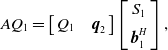
The key to the restarting technique is the Schur form
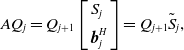 \begin{align}A{Q_j} = {Q_{j + 1}}\left[ {\begin{array}{*{20}{l}}{{S_j}}\\[5pt] {\boldsymbol{b}_j^H}\end{array}} \right] = {Q_{j + 1}}{\tilde S_j},\end{align}
where ${Q_{j + 1}} = \left[ {{Q_j}{\rm{\;\;}}{\boldsymbol{q}_{j + 1}}} \right]$
is an orthogonal matrix with
${Q_{j + 1}} = \left[ {{Q_j}{\rm{\;\;}}{\boldsymbol{q}_{j + 1}}} \right]$
is an orthogonal matrix with ${Q_1} = \left[ {{\boldsymbol{q}_1}} \right]$
,
${Q_1} = \left[ {{\boldsymbol{q}_1}} \right]$
, ${S_j}$
is a
${S_j}$
is a $j \times j$
upper-triangular matrix and
$j \times j$
upper-triangular matrix and $\boldsymbol{b}_j^H$
is a
$\boldsymbol{b}_j^H$
is a $1 \times j$
row vector. The eigenvalues of
$1 \times j$
row vector. The eigenvalues of ${S_j}$
, which are found along its diagonal, are good approximations to the largest eigenvalues of
${S_j}$
, which are found along its diagonal, are good approximations to the largest eigenvalues of $A$
, i.e. the wanted eigenvalues of
$A$
, i.e. the wanted eigenvalues of $J$
after shift-invert transformation, once the elements of
$J$
after shift-invert transformation, once the elements of $\boldsymbol{b}_j^H$
fall below a user-defined tolerance.
$\boldsymbol{b}_j^H$
fall below a user-defined tolerance.
Upon reaching some maximum specified subspace size $j = m$
, the Schur form is split into two parts, one consisting of the first
$j = m$
, the Schur form is split into two parts, one consisting of the first $t$
columns and the other consisting of the remaining
$t$
columns and the other consisting of the remaining $\left( {m - t} \right)$
columns, such that
$\left( {m - t} \right)$
columns, such that
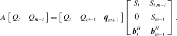 \begin{align}A\left[ {\begin{array}{l@{\quad}l}{{Q_t}} & {{Q_{m - t}}}\end{array}} \right] = \left[ {\begin{array}{c@{\quad}c@{\quad}c}{{Q_t}} & {{Q_{m - t}}}& {{\boldsymbol{q}_{m + 1}}}\end{array}} \right]\left[ {\begin{array}{c@{\quad}c}{{S_t}} & {{S_{t,m - t}}}\\[5pt] 0 & {{S_{m - t}}}\\[5pt] {\boldsymbol{b}_t^H}& {\boldsymbol{b}_{m - t}^H}\end{array}} \right].\end{align}
The restart technique simply involves discarding the last $\left( {m - t} \right)$
columns of
$\left( {m - t} \right)$
columns of ${Q_m}$
and
${Q_m}$
and ${S_m}$
yielding a contracted Schur form
${S_m}$
yielding a contracted Schur form
 \begin{align}A{Q_t} = \left[ {\begin{array}{c@{\quad}c}{{Q_t}} & {{\boldsymbol{q}_{m + 1}}}\end{array}} \right]\left[ {\begin{array}{c}{{S_t}}\\[5pt] {\boldsymbol{b}_t^H}\end{array}} \right] = {Q_{t + 1}}{\tilde S_t}.\end{align}
Note that vector ${\boldsymbol{q}_{m + 1}}$
is retained and re-labelled as
${\boldsymbol{q}_{m + 1}}$
is retained and re-labelled as ${\boldsymbol{q}_{t + 1}}$
to be consistent with the Schur form notation. The contraction procedure from
${\boldsymbol{q}_{t + 1}}$
to be consistent with the Schur form notation. The contraction procedure from ${S_m}$
to
${S_m}$
to ${S_t}$
is shown schematically in Fig. 1 for
${S_t}$
is shown schematically in Fig. 1 for $m = 5$
and
$m = 5$
and $t = 3$
. It was previously shown [Reference Stewart8] that this restart technique is equivalent to applying a polynomial filter,
$t = 3$
. It was previously shown [Reference Stewart8] that this restart technique is equivalent to applying a polynomial filter, $p\left( r \right) = \left( {r - {s_{t + 1}}} \right) \times \cdots \times \left( {r - {s_m}} \right)$
where
$p\left( r \right) = \left( {r - {s_{t + 1}}} \right) \times \cdots \times \left( {r - {s_m}} \right)$
where ${s_j}$
is the
${s_j}$
is the $j$
th diagonal element in
$j$
th diagonal element in ${S_m}$
. If the diagonal elements of
${S_m}$
. If the diagonal elements of ${S_m}$
are arranged such that the last
${S_m}$
are arranged such that the last $\left( {m - t} \right)$
elements belonged to the unwanted part of the spectrum, then the contraction procedure effectively purges the decomposition of the unwanted part of the spectrum.
$\left( {m - t} \right)$
elements belonged to the unwanted part of the spectrum, then the contraction procedure effectively purges the decomposition of the unwanted part of the spectrum.
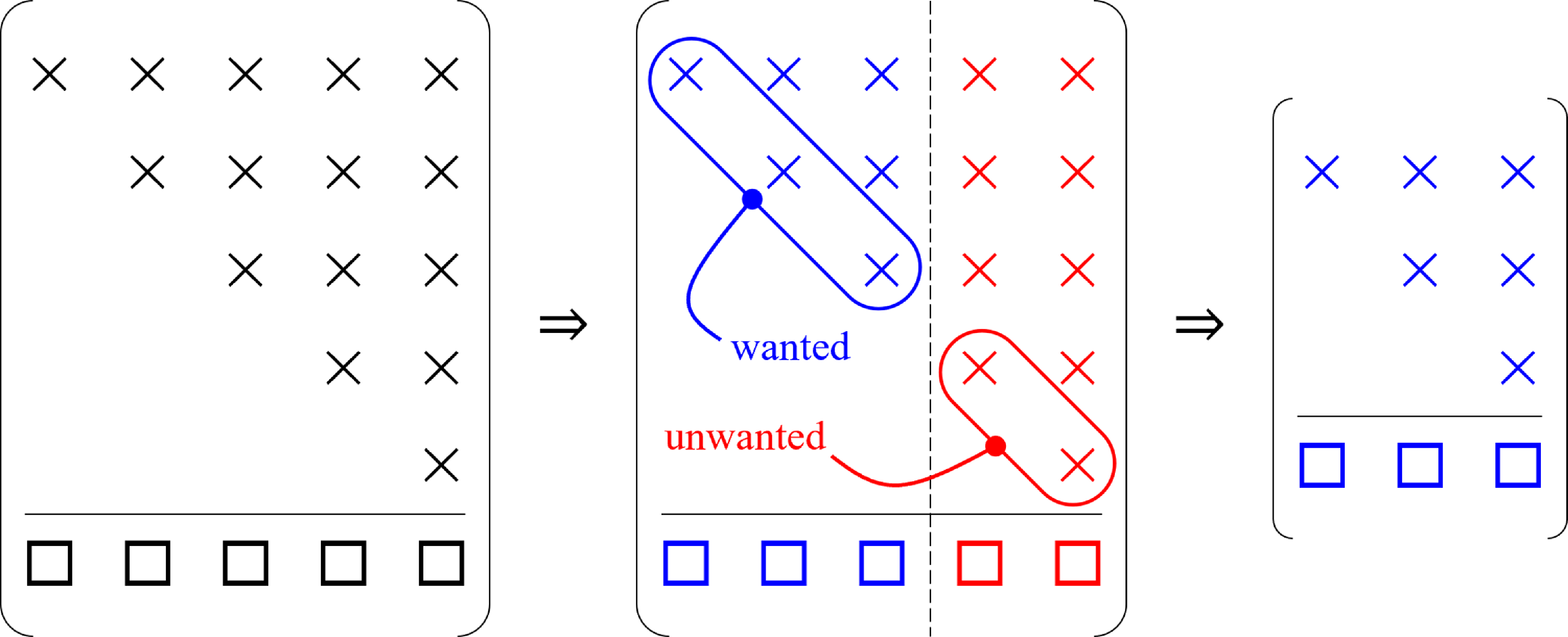
Figure 1. Schematic of ${\tilde S_m}$
during a restart for
${\tilde S_m}$
during a restart for $m = 5$
and
$m = 5$
and $t = 3$
.
$t = 3$
.
It is evident from the preceding discussion that it is crucial to maintain (or, at least, to be able to return to) the Schur form to benefit from the simple restarting technique. In the present implementation, the Schur form is preserved at the end of each Krylov–Schur iteration. The dense matrix operations required to do so are relatively inexpensive compared to the application of the linear operator $A$
which involves solving a large linear problem. Let us assume that we begin with the Schur form given in Equation (5). Performing an Arnoldi iteration on vector
$A$
which involves solving a large linear problem. Let us assume that we begin with the Schur form given in Equation (5). Performing an Arnoldi iteration on vector ${\boldsymbol{q}_{j + 1}}$
results in
${\boldsymbol{q}_{j + 1}}$
results in
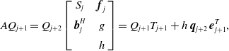 \begin{align}A{Q_{j + 1}} = {Q_{j + 2}}\left[ {\begin{array}{c@{\quad}c}{{S_j}} & {{\boldsymbol{f}_j}}\\[5pt] {\boldsymbol{b}_j^H} & g\\[5pt] {} & h\end{array}} \right] = {Q_{j + 1}}{T_{j + 1}} + h{\rm{\;}}{\boldsymbol{q}_{j + 2}}{\rm{\;}}\boldsymbol{e}_{j + 1}^T,\end{align}
where the $j \times 1$
column vector
$j \times 1$
column vector ${\boldsymbol{f}_j}$
and the scalars
${\boldsymbol{f}_j}$
and the scalars $g$
and
$g$
and $h$
are obtained by orthogonalising
$h$
are obtained by orthogonalising $A{\boldsymbol{q}_{j + 1}}$
over
$A{\boldsymbol{q}_{j + 1}}$
over ${Q_{j + 1}}$
. Since the Arnoldi iteration has disrupted the Schur form, we must perform a series of orthogonal similarity transformations to bring
${Q_{j + 1}}$
. Since the Arnoldi iteration has disrupted the Schur form, we must perform a series of orthogonal similarity transformations to bring ${T_{j + 1}}$
back to the Schur form [Reference Golub and Van Loan12]. First,
${T_{j + 1}}$
back to the Schur form [Reference Golub and Van Loan12]. First, ${T_{j + 1}}$
is brought into the upper-Hessenberg form
${T_{j + 1}}$
is brought into the upper-Hessenberg form ${H_{j + 1}} = V_1^H{T_{j + 1}}{V_1}$
using Householder reflections. Then,
${H_{j + 1}} = V_1^H{T_{j + 1}}{V_1}$
using Householder reflections. Then, ${H_{j + 1}}$
is brought into the complex Schur form
${H_{j + 1}}$
is brought into the complex Schur form ${S'_{\!\!j + 1}} = V_2^H{H_{j + 1}}{V_2}$
using the shifted QR algorithm [Reference Francis13, Reference Francis14]. Finally, the diagonal elements of the upper-triangular matrix
${S'_{\!\!j + 1}} = V_2^H{H_{j + 1}}{V_2}$
using the shifted QR algorithm [Reference Francis13, Reference Francis14]. Finally, the diagonal elements of the upper-triangular matrix ${S'_{\!\!j + 1}}$
are reordered in descending order of their absolute values using special orthogonal matrices (see Appendix B) which yields the ordered Schur form
${S'_{\!\!j + 1}}$
are reordered in descending order of their absolute values using special orthogonal matrices (see Appendix B) which yields the ordered Schur form ${S_{j + 1}} = V_3^H{S'_{\!\!j + 1}}{V_3}$
. The reordering is necessary so that the restart discards information about the eigenvalues farthest away from
${S_{j + 1}} = V_3^H{S'_{\!\!j + 1}}{V_3}$
. The reordering is necessary so that the restart discards information about the eigenvalues farthest away from $\sigma $
. The combined effect of these three operations can be represented by a single similarity transformation
$\sigma $
. The combined effect of these three operations can be represented by a single similarity transformation ${S_{j + 1}} = {V^H}{T_{j + 1}}V$
where
${S_{j + 1}} = {V^H}{T_{j + 1}}V$
where $V = {V_1}{V_2}{V_3}$
is an orthogonal matrix. Substituting
$V = {V_1}{V_2}{V_3}$
is an orthogonal matrix. Substituting ${T_{j + 1}} = V{S_{j + 1}}{V^H}$
into Equation (8) results in
${T_{j + 1}} = V{S_{j + 1}}{V^H}$
into Equation (8) results in
 \begin{align}A{Q_{j + 1}} = {Q_{j + 1}}\left( {V{S_{j + 1}}{V^H}} \right) + h{\rm{\;}}{\boldsymbol{q}_{j + 2}}{\rm{\;}}\boldsymbol{e}_{j + 1}^T.\end{align}
Multiplying both sides of the latter equation by $V$
from the right and setting
$V$
from the right and setting ${Q_{j + 1}} = {Q_{j + 1}}V$
and
${Q_{j + 1}} = {Q_{j + 1}}V$
and $b_{j + 1}^H = he_{j + 1}^TV$
results in
$b_{j + 1}^H = he_{j + 1}^TV$
results in
 \begin{align}A{Q_{j + 1}} = {Q_{j + 1}}{S_{j + 1}} + {\boldsymbol{q}_{j + 2}}{\rm{\;}}\boldsymbol{b}_{j + 1}^H\end{align}
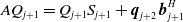
which is the sought-after Schur form. The expansion from ${S_j}$
to
${S_j}$
to ${S_{j + 1}}$
during the Krylov–Schur iteration for
${S_{j + 1}}$
during the Krylov–Schur iteration for $j = 3$
is shown schematically in Fig. 2. Last but not least, we observe that the Arnoldi iteration is equivalent to a Krylov–Schur iteration for
$j = 3$
is shown schematically in Fig. 2. Last but not least, we observe that the Arnoldi iteration is equivalent to a Krylov–Schur iteration for $j = 0$
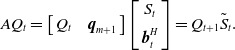
. Starting from a random unit vector
$j = 0$
. Starting from a random unit vector ${\boldsymbol{q}_1}$
, we perform an Arnoldi iteration to obtain
${\boldsymbol{q}_1}$
, we perform an Arnoldi iteration to obtain
 \begin{align}A{Q_1} = \left[ {\begin{array}{c@{\quad}c}{{Q_1}} & {{\boldsymbol{q}_2}}\end{array}} \right]\left[ {\begin{array}{c}{{S_1}}\\[5pt] {\boldsymbol{b}_1^H}\end{array}} \right],\end{align}
where ${S_1}$
and
${S_1}$
and $\boldsymbol{b}_1^H$
are just scalars and
$\boldsymbol{b}_1^H$
are just scalars and ${Q_1} = \left[ {{\boldsymbol{q}_1}} \right]$
. Nonetheless, it can be seen that Equation (11) is in the Schur form and requires no further transformation.
${Q_1} = \left[ {{\boldsymbol{q}_1}} \right]$
. Nonetheless, it can be seen that Equation (11) is in the Schur form and requires no further transformation.
The desired $k \le j$
eigenvectors of
$k \le j$
eigenvectors of $A$
can be approximated from the Schur form as
$A$
can be approximated from the Schur form as
 \begin{align}{{W}_k} = {Q_k}{P_k},\end{align}
where matrix ${{W}_k} = \left[ {{{\widehat {\boldsymbol{W}}}_1}{\rm{\;\;}} \ldots {\rm{\;}}{{\widehat {\boldsymbol{W}}}_k}} \right]$
contains the approximate eigenvectors (Ritz vectors) of
${{W}_k} = \left[ {{{\widehat {\boldsymbol{W}}}_1}{\rm{\;\;}} \ldots {\rm{\;}}{{\widehat {\boldsymbol{W}}}_k}} \right]$
contains the approximate eigenvectors (Ritz vectors) of $A$
and
$A$
and ${P_k} = \left[ {{\boldsymbol{p}_1}{\rm{\;\;}} \ldots {\rm{\;\;}}{\boldsymbol{p}_k}} \right]$
is a
${P_k} = \left[ {{\boldsymbol{p}_1}{\rm{\;\;}} \ldots {\rm{\;\;}}{\boldsymbol{p}_k}} \right]$
is a $k \times k$
matrix whose columns are the eigenvectors of
$k \times k$
matrix whose columns are the eigenvectors of ${S_k}$
which is the
${S_k}$
which is the $k \times k$
matrix formed from the top-left corner of
$k \times k$
matrix formed from the top-left corner of ${S_j}$
. The eigenvectors
${S_j}$
. The eigenvectors ${\boldsymbol{p}_i}$
for
${\boldsymbol{p}_i}$
for $i = 1 \ldots k$
can be computed from the relationship
$i = 1 \ldots k$
can be computed from the relationship ${S_k}{\boldsymbol{p}_i} = {s_i}{\boldsymbol{p}_i}$
combined with the fact that both
${S_k}{\boldsymbol{p}_i} = {s_i}{\boldsymbol{p}_i}$
combined with the fact that both ${S_k}$
and
${S_k}$
and ${P_k}$
are upper-triangular.
${P_k}$
are upper-triangular.
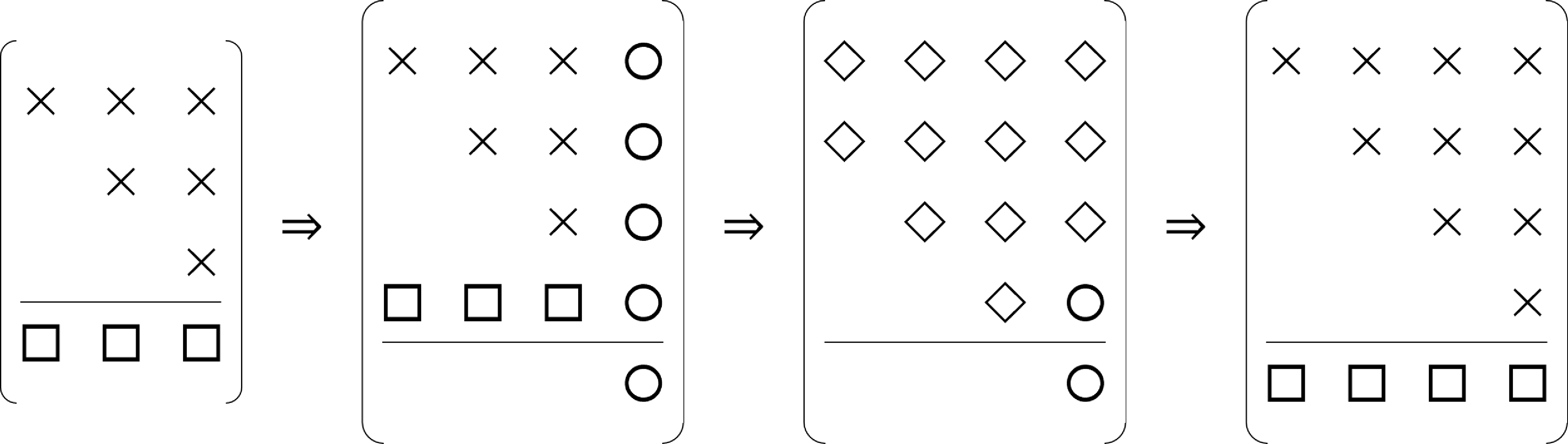
Figure 2. Schematic of ${\tilde S_k}$
during a Krylov-Schur iteration for
${\tilde S_k}$
during a Krylov-Schur iteration for $j = 3$
.
$j = 3$
.
The error in the $i$
th eigenvector approximation can be computed as
$i$
th eigenvector approximation can be computed as
 \begin{align}{\varepsilon _i} = \parallel A{\widehat {\boldsymbol{W}}_i} - {s_i}{\widehat {\boldsymbol{W}}_i}{\parallel _2}.\end{align}
Substituting ${\widehat {\boldsymbol{W}}_i} = {Q_k}{\boldsymbol{p}_i}$
and
${\widehat {\boldsymbol{W}}_i} = {Q_k}{\boldsymbol{p}_i}$
and ${s_i}{\boldsymbol{p}_i} = {S_k}{\boldsymbol{p}_i}$
into Equation (13) leads to
${s_i}{\boldsymbol{p}_i} = {S_k}{\boldsymbol{p}_i}$
into Equation (13) leads to
 \begin{align}{\varepsilon _i} = \parallel \left( {A{Q_k} - {Q_k}{S_k}} \right){\boldsymbol{p}_i}{\parallel _2} = \parallel {\boldsymbol{q}_{k + 1}}\boldsymbol{b}_k^H{\boldsymbol{p}_i}{\parallel _2} = \parallel \boldsymbol{b}_k^H{\boldsymbol{p}_i}{\parallel _2}\end{align}
where ${\boldsymbol{b}_k}$
is formed from the first
${\boldsymbol{b}_k}$
is formed from the first $k$
elements of
$k$
elements of ${\boldsymbol{b}_j}$
. The second equality in Equation (14) arises from the Schur form itself and the last equality is due to
${\boldsymbol{b}_j}$
. The second equality in Equation (14) arises from the Schur form itself and the last equality is due to ${\boldsymbol{q}_{k + 1}}$
having unit norm. The approximation errors are computed at the end of each Krylov–Schur iteration. Once the
${\boldsymbol{q}_{k + 1}}$
having unit norm. The approximation errors are computed at the end of each Krylov–Schur iteration. Once the $i$
th error norm has dropped below a prescribed threshold value (e.g.
$i$
th error norm has dropped below a prescribed threshold value (e.g. ${10^{ - 10}}$
), the eigenpair is deemed to have converged and is locked by setting the
${10^{ - 10}}$
), the eigenpair is deemed to have converged and is locked by setting the $i$
th component of
$i$
th component of ${\boldsymbol{b}_j}$
to zero. Subsequent transformations on
${\boldsymbol{b}_j}$
to zero. Subsequent transformations on ${S_j}$
are only applied from the
${S_j}$
are only applied from the $\left( {i + 1} \right)$
th row and column leaving the top-left
$\left( {i + 1} \right)$
th row and column leaving the top-left $i \times i$
part of
$i \times i$
part of ${S_j}$
and the first
${S_j}$
and the first $i$
columns of
$i$
columns of
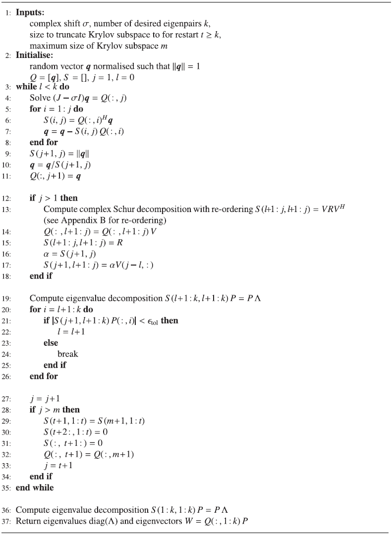
 ${Q_j}$
unchanged. The computation is terminated when the last desired eigenpair has converged. The entire algorithm is summarised in Appendix A. Note that we have used Fortran indexing with the indices starting from 1.
${Q_j}$
unchanged. The computation is terminated when the last desired eigenpair has converged. The entire algorithm is summarised in Appendix A. Note that we have used Fortran indexing with the indices starting from 1.
3.0 Methodology
3.1 Non-linear steady-state problem
The steady-state problem![]() was solved first since the Jacobian operator
was solved first since the Jacobian operator $J = - \partial \boldsymbol{R}/\partial {\boldsymbol{W}}$
for the eigenvalue problem must be computed about a suitable reference state
$J = - \partial \boldsymbol{R}/\partial {\boldsymbol{W}}$
for the eigenvalue problem must be computed about a suitable reference state![]() . The non-linear flow solutions were computed in CODA using the implicit backward Euler scheme with local time stepping until the density residual norm dropped by 10 orders of magnitude. No special solution stabilisation techniques (such as selective frequency damping) were required to achieve convergence herein. Courant–Friedrich–Levy (CFL) number ramping of the local time steps was employed to accelerate non-linear convergence. The linear system at each outer iteration was solved using a restarted generalised minimal residual (GMRES) solver [Reference Saad and Schultz15] until the linear residual norm dropped by one order of magnitude. The solver used a maximum of 100 Krylov vectors before restart with 50 iterations of a block-Jacobi solver as preconditioner. The GMRES solver utilises a matrix-free approach using AD to compute the matrix-vector products
. The non-linear flow solutions were computed in CODA using the implicit backward Euler scheme with local time stepping until the density residual norm dropped by 10 orders of magnitude. No special solution stabilisation techniques (such as selective frequency damping) were required to achieve convergence herein. Courant–Friedrich–Levy (CFL) number ramping of the local time steps was employed to accelerate non-linear convergence. The linear system at each outer iteration was solved using a restarted generalised minimal residual (GMRES) solver [Reference Saad and Schultz15] until the linear residual norm dropped by one order of magnitude. The solver used a maximum of 100 Krylov vectors before restart with 50 iterations of a block-Jacobi solver as preconditioner. The GMRES solver utilises a matrix-free approach using AD to compute the matrix-vector products $J{\boldsymbol{x}}$
exactly for an arbitrary real (or complex) vector
$J{\boldsymbol{x}}$
exactly for an arbitrary real (or complex) vector $\boldsymbol{x}$
. The preconditioner, on the other hand, uses an explicitly formed matrix whose block-diagonal (i.e. the coupled governing equations for all spatial degrees of freedom within a cell) is factorised using LU decomposition. The explicit matrix is formed with the help of AD as well using compact stencils. The compact stencil for a cell consists of the cell and its immediate face-neighbours only. Since DG schemes use compact stencils, the explicit matrix is exact. For the FV scheme, which relies on extended stencils, the explicit matrix is approximate and essentially only first-order accurate. However, this is not a severe disadvantage. In fact, the approximate matrix is more diagonally dominant leading to improved stability of the preconditioner [Reference McCracken, Da Ronch, Timme and Badcock16].
$\boldsymbol{x}$
. The preconditioner, on the other hand, uses an explicitly formed matrix whose block-diagonal (i.e. the coupled governing equations for all spatial degrees of freedom within a cell) is factorised using LU decomposition. The explicit matrix is formed with the help of AD as well using compact stencils. The compact stencil for a cell consists of the cell and its immediate face-neighbours only. Since DG schemes use compact stencils, the explicit matrix is exact. For the FV scheme, which relies on extended stencils, the explicit matrix is approximate and essentially only first-order accurate. However, this is not a severe disadvantage. In fact, the approximate matrix is more diagonally dominant leading to improved stability of the preconditioner [Reference McCracken, Da Ronch, Timme and Badcock16].
Spatial discretisation was performed herein using both FV and DG methods. In the FV method, the solution is computed as the cell averages of the conservative variables, i.e. each cell represents one degree of freedom (DOF) per variable. In the DG method, each variable is represented as an $n$
th order polynomial in three dimensions where we limit our interest herein to
$n$
th order polynomial in three dimensions where we limit our interest herein to $n \in \left[ {2, \ldots ,8} \right]$
. Therefore, each cell represents
$n \in \left[ {2, \ldots ,8} \right]$
. Therefore, each cell represents ${{\rm{\;}}^{n + 2}}{C_3} = \left( {n + 2} \right)\left( {n + 1} \right)n/6$
DOF for each variable where
${{\rm{\;}}^{n + 2}}{C_3} = \left( {n + 2} \right)\left( {n + 1} \right)n/6$
DOF for each variable where ${{\rm{\;}}^n}{C_k}$
is the binomial coefficient. For the two-dimensional cases considered in this study, the DOF per cell can be significantly reduced (only
${{\rm{\;}}^n}{C_k}$
is the binomial coefficient. For the two-dimensional cases considered in this study, the DOF per cell can be significantly reduced (only ${{\rm{\;}}^{n + 1}}{C_2}$
) since the third dimension is redundant. However, as CODA does not currently support such a two-dimensional DG formulation, the full three-dimensional formulation was used despite the redundancy.
${{\rm{\;}}^{n + 1}}{C_2}$
) since the third dimension is redundant. However, as CODA does not currently support such a two-dimensional DG formulation, the full three-dimensional formulation was used despite the redundancy.
The inviscid fluxes were computed using the Roe scheme with no entropy fix based on the face values. In the FV method, the face values at the face centroids were first approximated using distance-weighted interpolation of the face-adjacent neighbours’ cell averages. Then, cell average gradients were computed from the approximate face values using the Green–Gauss method. The final face values were computed as a linear function of the cell average values and gradients. In the DG method, the face values were computed by evaluating the polynomial at the face quadrature points. The flux over each face was integrated as a weighted average of the fluxes computed at the quadrature points. The viscous fluxes were computed based on face gradients. In the FV method, the face gradients were computed as the distance-weighted averages of the neighbouring cell average gradients with edge-normal augmentation [Reference Schwöppe and Diskin17]. In the DG method, the viscous fluxes were computed using the second approach proposed by Bassi and Rebay known as the BR2 scheme [Reference Bassi, Crivellini, Rebay and Savini18].
3.2 Eigenvalue problem
With the steady-state solution computed, the Krylov–Schur algorithm, implemented as part of this work, was used to determine the rightmost (in the complex plane) eigenpair. Observe that the chosen flow conditions are such that $\Re \mathfrak{e}\left( {{\lambda _J}} \right) \gt 0$
for the leading eigenmode and it describes unstable flow, specifically vortex shedding in the wake behind bluff bodies. In the Krylov–Schur algorithm, unless otherwise specified, the subspace was allowed to expand to a maximum size
$\Re \mathfrak{e}\left( {{\lambda _J}} \right) \gt 0$
for the leading eigenmode and it describes unstable flow, specifically vortex shedding in the wake behind bluff bodies. In the Krylov–Schur algorithm, unless otherwise specified, the subspace was allowed to expand to a maximum size $m = 20$
before a restart, when it was truncated to
$m = 20$
before a restart, when it was truncated to $t = 5$
. The linear system of the form
$t = 5$
. The linear system of the form $\left( {J - \sigma I} \right)\boldsymbol{x} = \boldsymbol{q}$
in each Krylov–Schur iteration was solved using the GMRES solver with the same settings as that used for the steady-state problem except that 100 block-Jacobi iterations were used as preconditioner. CODA’s linear algebra library Spliss can deal with the necessary complex algebra and further details on solving the complex linear problems can be found in previous work [Reference Vevek, Timme, Pattinson, Stickan and Büchner9]. The shift
$\left( {J - \sigma I} \right)\boldsymbol{x} = \boldsymbol{q}$
in each Krylov–Schur iteration was solved using the GMRES solver with the same settings as that used for the steady-state problem except that 100 block-Jacobi iterations were used as preconditioner. CODA’s linear algebra library Spliss can deal with the necessary complex algebra and further details on solving the complex linear problems can be found in previous work [Reference Vevek, Timme, Pattinson, Stickan and Büchner9]. The shift $\sigma $
was chosen close to the unstable eigenvalue based on the prior knowledge of the physics and numerical experiments to ensure fast convergence. During the numerical experiments, the approximation error of a converged eigenpair was observed to be directly dependent on the convergence of the linear solver in each Krylov–Schur iteration. To achieve a relative approximation error below
$\sigma $
was chosen close to the unstable eigenvalue based on the prior knowledge of the physics and numerical experiments to ensure fast convergence. During the numerical experiments, the approximation error of a converged eigenpair was observed to be directly dependent on the convergence of the linear solver in each Krylov–Schur iteration. To achieve a relative approximation error below ${10^{ - 10}}$
, the linear system in each Krylov–Schur iteration was solved until the residual norm dropped below
${10^{ - 10}}$
, the linear system in each Krylov–Schur iteration was solved until the residual norm dropped below ${10^{ - 10}}$
.
${10^{ - 10}}$
.
4.0 Results and discussion
4.1 Laminar flow past circular cylinder
We first consider laminar $M = 0.2$
flow past a circular cylinder as a validation case, which has been widely documented in the literature. The unstructured grid shown in Fig. 3 was used, which includes a quasi-structured near-field region and a total of 11,638 cells (corresponding to 9,743 vertices in a two-dimensional set-up). The computational domain has a radial extent of
$M = 0.2$
flow past a circular cylinder as a validation case, which has been widely documented in the literature. The unstructured grid shown in Fig. 3 was used, which includes a quasi-structured near-field region and a total of 11,638 cells (corresponding to 9,743 vertices in a two-dimensional set-up). The computational domain has a radial extent of $100D$
, where
$100D$
, where $D = 1$
is the diameter of the circular cylinder, and a unit extent in the spanwise direction. The far-field view in Fig. 3(a) shows the wake refinement. The quasi-structured grid around the cylinder has a first wall-normal cell spacing of
$D = 1$
is the diameter of the circular cylinder, and a unit extent in the spanwise direction. The far-field view in Fig. 3(a) shows the wake refinement. The quasi-structured grid around the cylinder has a first wall-normal cell spacing of $D/1000$
and becomes unstructured starting at a radial distance of
$D/1000$
and becomes unstructured starting at a radial distance of $4.25D$
from the origin as seen in Fig. 3(b).
$4.25D$
from the origin as seen in Fig. 3(b).
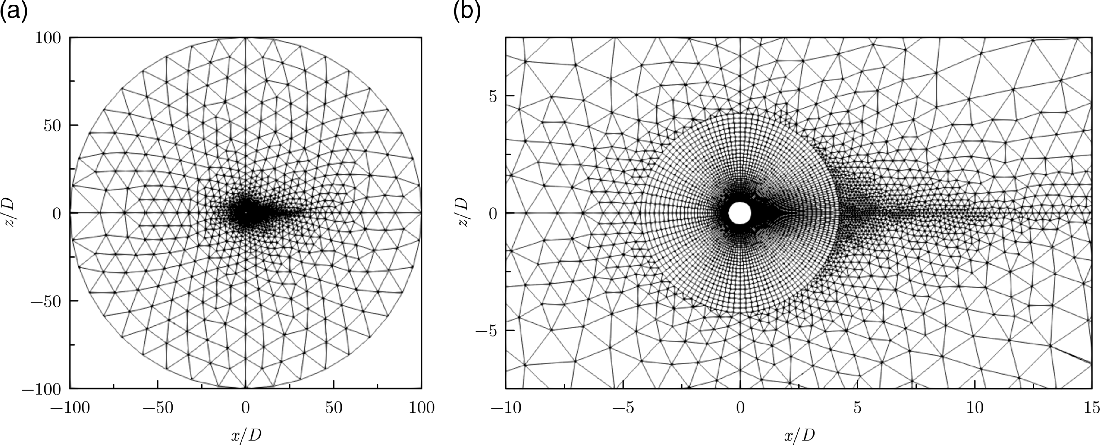
Figure 3. Grid used for laminar flow past circular cylinder case.
The test case was computed at a slightly supercritical Reynolds number $Re = 50$
to ensure the presence of an unstable mode linked to von Kármán vortex shedding. The complex shift,
$Re = 50$
to ensure the presence of an unstable mode linked to von Kármán vortex shedding. The complex shift, $\sigma = i0.75$
, was chosen such that its imaginary part was close to the critical vortex-shedding frequency, which relies on engineering insight gained from the past study of bluff body aerodynamics. While no attempt was made in this study to assess the impact of the spectral distance between shift and wanted eigenvalue on the performance of the eigenmode solver, it is clear that there is a compromise between the rate of convergence of the shift-inverted Krylov–Schur algorithm, which improves with a reduced spectral distance, and the numerical properties of the shifted linear system, which becomes increasingly singular and hence more difficult to solve with reduced spectral distance. Both the direct eigenvalue problem in Equation (2) and the adjoint eigenvalue problem in Equation (3) were solved using CODA and TAU.Footnote
1
For CODA, only the FV method was used for this case.
$\sigma = i0.75$
, was chosen such that its imaginary part was close to the critical vortex-shedding frequency, which relies on engineering insight gained from the past study of bluff body aerodynamics. While no attempt was made in this study to assess the impact of the spectral distance between shift and wanted eigenvalue on the performance of the eigenmode solver, it is clear that there is a compromise between the rate of convergence of the shift-inverted Krylov–Schur algorithm, which improves with a reduced spectral distance, and the numerical properties of the shifted linear system, which becomes increasingly singular and hence more difficult to solve with reduced spectral distance. Both the direct eigenvalue problem in Equation (2) and the adjoint eigenvalue problem in Equation (3) were solved using CODA and TAU.Footnote
1
For CODA, only the FV method was used for this case.
But first, to demonstrate the implementation of the Krylov–Schur algorithm in CODA and the convergence characteristics of the cylinder validation case, Fig. 4 shows details of the computation of the three direct modes closest to the chosen shift. As expected, the modes converge consecutively with increasing spectral distance, $\left| {{\lambda _J} - \sigma } \right|$
. Three parameter settings of the Krylov–Schur algorithm were specified (in terms of maximum and truncated subspace size denoted
$\left| {{\lambda _J} - \sigma } \right|$
. Three parameter settings of the Krylov–Schur algorithm were specified (in terms of maximum and truncated subspace size denoted $m$
and
$m$
and $t$
, respectively); no truncation,
$t$
, respectively); no truncation, $\left[ {m = 10,{\rm{\;}}t = 5} \right]$
and
$\left[ {m = 10,{\rm{\;}}t = 5} \right]$
and $\left[ {m = 6,{\rm{\;}}t = 3} \right]$
. It is evident that the leading, well-isolated wake mode converges in 12 iterations regardless of the subspace size after restart. Modes 2 and 3 are more difficult to converge; these modes are close to a large number of nondescript, spurious modes [Reference Timme, Badcock, Wu and Spence21]. Without subspace truncation, these modes both converge in just under 60 iterations. For the setting with the bigger limited subspace, convergence is still straightforward in just over 80 iterations. Convergence is slow using the final setting, with the algorithm locking onto the incorrect modes repeatedly. Nevertheless, eventually the sought modes are converged in 170 and 700 iterations, respectively. Essentially, too small a subspace is insufficient for non-isolated modes.
$\left[ {m = 6,{\rm{\;}}t = 3} \right]$
. It is evident that the leading, well-isolated wake mode converges in 12 iterations regardless of the subspace size after restart. Modes 2 and 3 are more difficult to converge; these modes are close to a large number of nondescript, spurious modes [Reference Timme, Badcock, Wu and Spence21]. Without subspace truncation, these modes both converge in just under 60 iterations. For the setting with the bigger limited subspace, convergence is still straightforward in just over 80 iterations. Convergence is slow using the final setting, with the algorithm locking onto the incorrect modes repeatedly. Nevertheless, eventually the sought modes are converged in 170 and 700 iterations, respectively. Essentially, too small a subspace is insufficient for non-isolated modes.
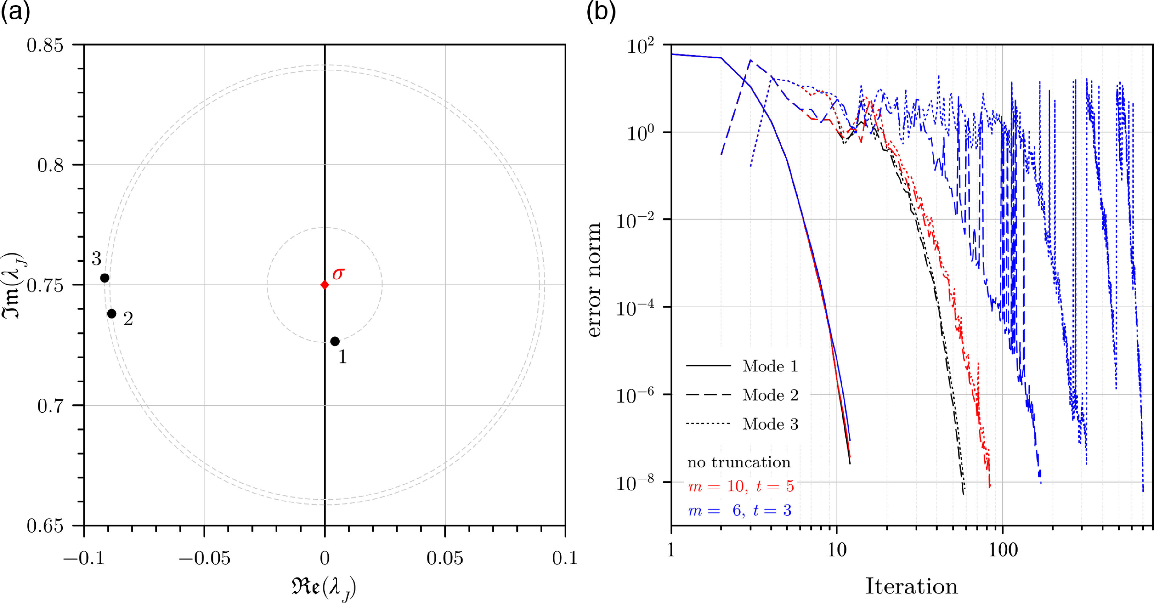
Figure 4. Convergence characteristics of three direct modes closest to chosen shift for laminar flow past circular cylinder case using CODA.
The leading, physically meaningful, non-dimensional eigenvalues ${\lambda _J}$
(made non-dimensional using
${\lambda _J}$
(made non-dimensional using $D$
and free-stream velocity
$D$
and free-stream velocity ${U_\infty }$
) of the von Kármán wake mode computed by CODA and TAU are
${U_\infty }$
) of the von Kármán wake mode computed by CODA and TAU are $0.0042507 + i0.72656$
and
$0.0042507 + i0.72656$
and $0.015829 + i0.73105$
, respectively. The positive real parts of
$0.015829 + i0.73105$
, respectively. The positive real parts of ${\lambda _J}$
indicate that the modes are indeed unstable. Overall, the results for
${\lambda _J}$
indicate that the modes are indeed unstable. Overall, the results for ${\lambda _J}$
are quite close to the numerical predictions by e.g. Crouch et al. [Reference Crouch, Garbaruk and Magidov1] and Fabre et al. [Reference Fabre, Citro, Ferreira Sabino, Bonnefis, Sierra, Giannetti and Pigou22] based on similar stability analyses. The real parts of the streamwise momentum component
${\lambda _J}$
are quite close to the numerical predictions by e.g. Crouch et al. [Reference Crouch, Garbaruk and Magidov1] and Fabre et al. [Reference Fabre, Citro, Ferreira Sabino, Bonnefis, Sierra, Giannetti and Pigou22] based on similar stability analyses. The real parts of the streamwise momentum component $\widehat{\rho u}$
of the eigenvectors are plotted in Fig. 5. The eigenvectors were scaled such that the maximum of the
$\widehat{\rho u}$
of the eigenvectors are plotted in Fig. 5. The eigenvectors were scaled such that the maximum of the $\widehat{\rho u}$
component has a value of
$\widehat{\rho u}$
component has a value of $1 + i0$
, i.e. a maximum amplitude of one with zero phase. The direct modes exhibit the well-known vortex shedding pattern downstream of the cylinder. The regions of high amplitudes of the adjoint modes highlight the locations where a harmonic forcing has the greatest effect on the global flowfield. It can be seen that the modal features agree qualitatively between the codes and also with existing literature in the field. Obviously, the coarseness of the chosen mesh to demonstrate the implementation of the methods would not allow a fully mesh-converged solution to be identified. This is exemplified by the streamwise position in the cylinder wake of the maximum cross-stream momentum component of the direct mode found at approximately
$1 + i0$
, i.e. a maximum amplitude of one with zero phase. The direct modes exhibit the well-known vortex shedding pattern downstream of the cylinder. The regions of high amplitudes of the adjoint modes highlight the locations where a harmonic forcing has the greatest effect on the global flowfield. It can be seen that the modal features agree qualitatively between the codes and also with existing literature in the field. Obviously, the coarseness of the chosen mesh to demonstrate the implementation of the methods would not allow a fully mesh-converged solution to be identified. This is exemplified by the streamwise position in the cylinder wake of the maximum cross-stream momentum component of the direct mode found at approximately $x = 14.6D$
for CODA and
$x = 14.6D$
for CODA and $x = 10.8D$
for TAU. Compare these with a maximum at approximately
$x = 10.8D$
for TAU. Compare these with a maximum at approximately $25D$
for more mesh-converged results [Reference Sipp and Lebedev23]. To address this point, the second test case of a square cylinder in laminar flow with a more detailed assessment is discussed next.
$25D$
for more mesh-converged results [Reference Sipp and Lebedev23]. To address this point, the second test case of a square cylinder in laminar flow with a more detailed assessment is discussed next.
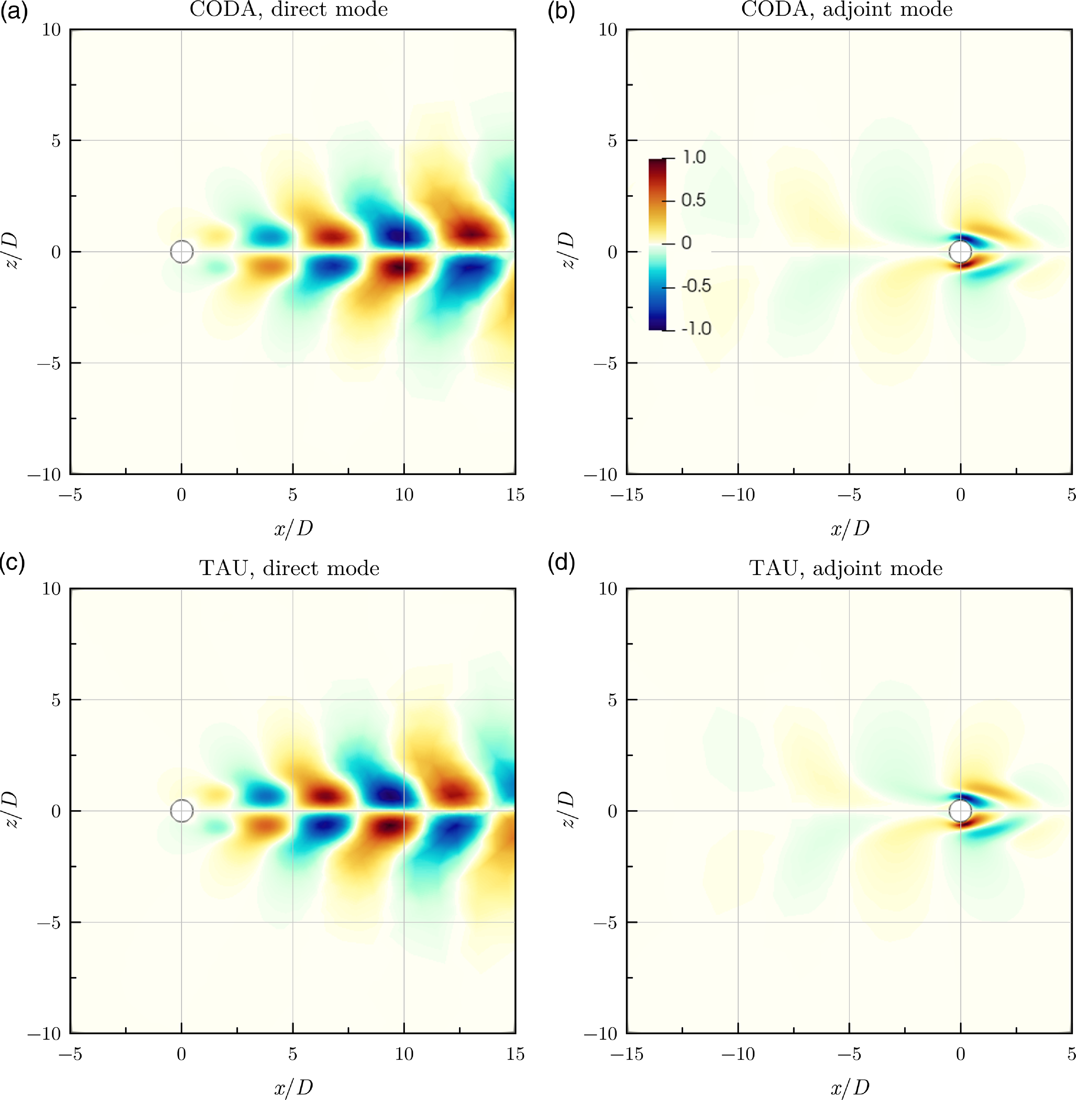
Figure 5. Streamwise momentum components of unstable direct and adjoint global modes for laminar flow past circular cylinder case.
4.2 Laminar flow past square cylinder
We now consider the case of laminar $M = 0.2$
flow past a square cylinder at
$M = 0.2$
flow past a square cylinder at $Re = 50$
, with a special focus on the high-order DG scheme in CODA. When using high-order DG schemes, it becomes necessary to use high-order grids to represent the curved geometries to achieve optimal accuracy [Reference Hartmann and Leicht24]. However, since a square cylinder has no curves, it can be represented exactly (and easily) with linear grids. Hence, the added complexity of generating high-order grids was avoided for this case. All CODA cases were computed on a single compute node that comprises 384 GB of memory and two Intel Xeon Gold 6230 (Cascade Lake) central processing units (CPUs) each consisting of 20 hardware cores. The cases were run using two MPI processes with 20 OpenMP threads per process.
$Re = 50$
, with a special focus on the high-order DG scheme in CODA. When using high-order DG schemes, it becomes necessary to use high-order grids to represent the curved geometries to achieve optimal accuracy [Reference Hartmann and Leicht24]. However, since a square cylinder has no curves, it can be represented exactly (and easily) with linear grids. Hence, the added complexity of generating high-order grids was avoided for this case. All CODA cases were computed on a single compute node that comprises 384 GB of memory and two Intel Xeon Gold 6230 (Cascade Lake) central processing units (CPUs) each consisting of 20 hardware cores. The cases were run using two MPI processes with 20 OpenMP threads per process.
The square cylinder was computed using seven structured grids (labelled as L0 to L6) with levels of varying refinement. A systematic global refinement approach with halving the mesh spacing and doubling the cell count in each spatial dimension was chosen. Thus, each new level has approximately four times as many cells as the previous level. The number of DOF per equation is listed in Table 1 for the FV schemes in TAU (vertex-centred) and CODA (cell-centred) and for the DG schemes in CODA for the cases discussed herein. The number of DOF for DG schemes is computed for the three-dimensional formulation including the spanwise direction which is redundant for the two-dimensional square cylinder case. Far-field and near-field views of grids L0 and L2 are shown in Fig. 6. The computational domain extends to a circular far-field distance of approximately $200D$
where
$200D$
where $D = 1$
is the length of the side of the square cylinder. DG schemes were employed in this study on grids L0 to L3 only, which is instructive when comparing with standard FV results. On grid L0, DG computations were performed from second order up to the maximum (currently) available order of eight. On grids L1 through L3, DG computations were performed from second order up to (at least) the minimum order that is needed for the lift coefficient
$D = 1$
is the length of the side of the square cylinder. DG schemes were employed in this study on grids L0 to L3 only, which is instructive when comparing with standard FV results. On grid L0, DG computations were performed from second order up to the maximum (currently) available order of eight. On grids L1 through L3, DG computations were performed from second order up to (at least) the minimum order that is needed for the lift coefficient ${C_L}$
to become smaller than (an arbitrarily chosen)
${C_L}$
to become smaller than (an arbitrarily chosen) ${10^{ - 8}}$
in magnitude. Note that the theoretical lift coefficient for this symmetrical case is zero. Hence, deviation from the theoretical value is indicative of the adequacy of the spatial resolution for a given scheme.
${10^{ - 8}}$
in magnitude. Note that the theoretical lift coefficient for this symmetrical case is zero. Hence, deviation from the theoretical value is indicative of the adequacy of the spatial resolution for a given scheme.
Table 1. Degrees of freedom per equation for laminar flow past square cylinder cases discussed herein; underlined cases are not further visualised for clarity
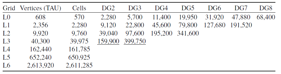
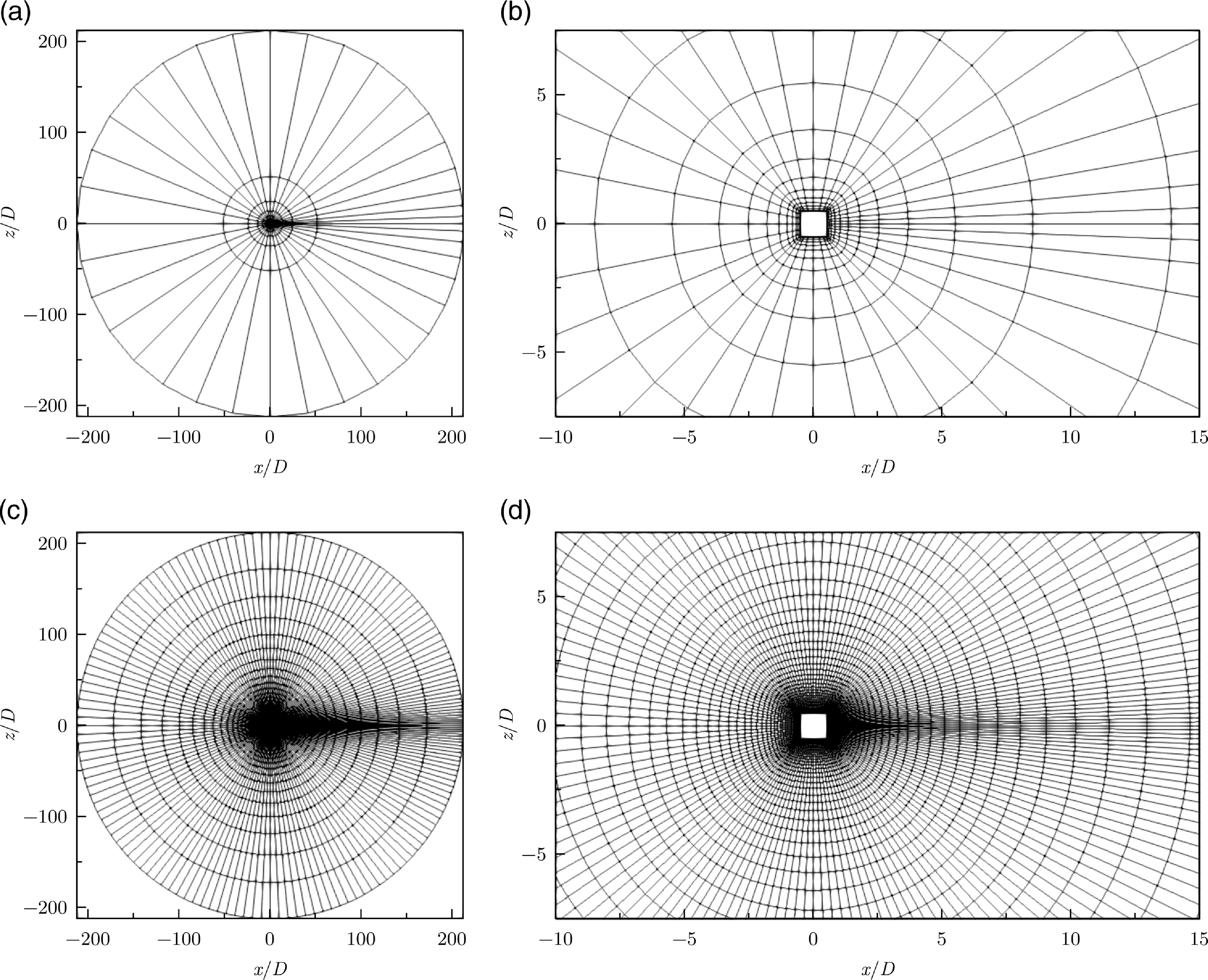
Figure 6. Grids L0 (top) and L2 (bottom) used for laminar flow past square cylinder case.
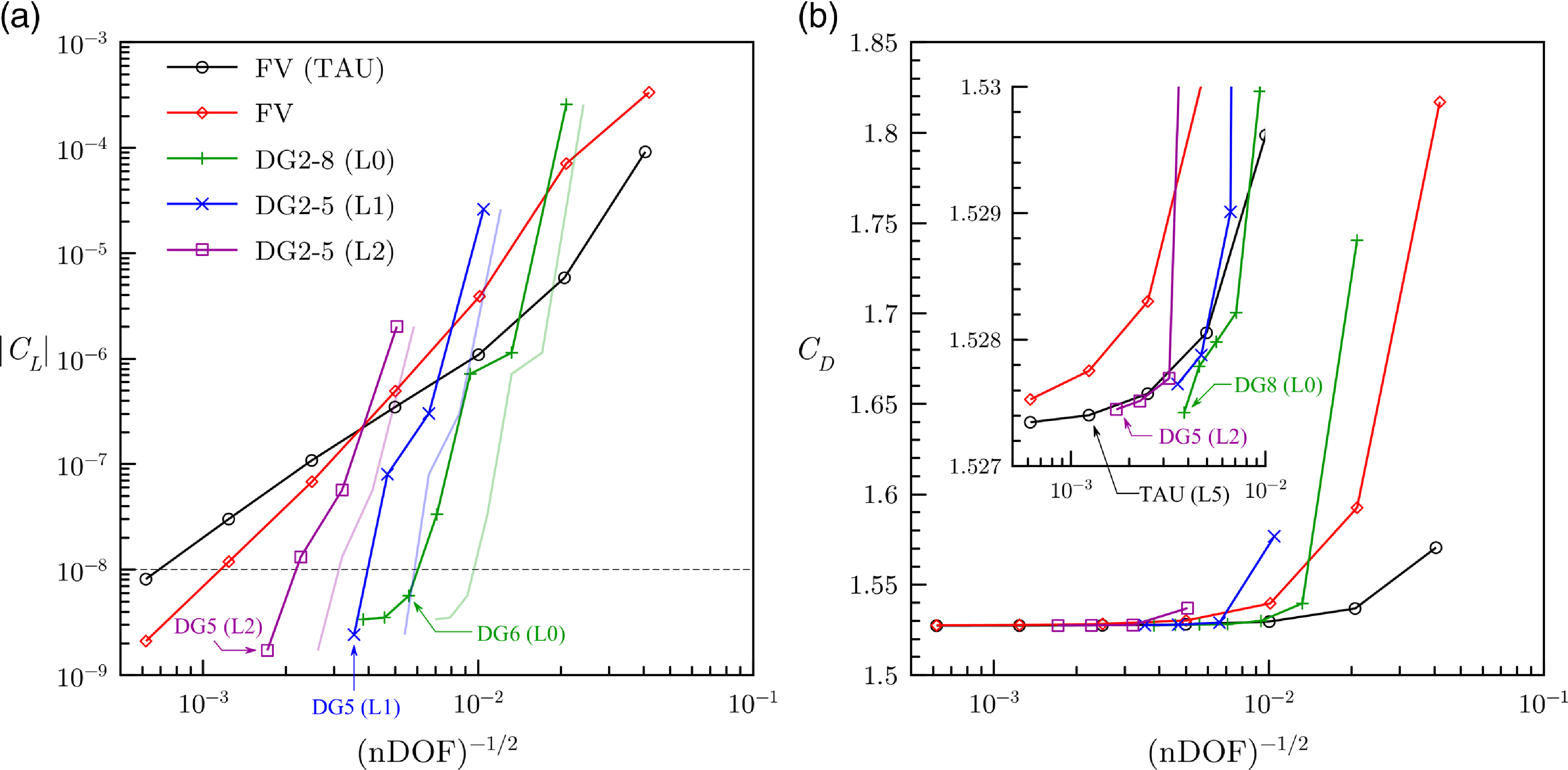
Figure 7. Steady-state lift and drag coefficients for laminar flow past square cylinder case. Faint lines for lift coefficients are plotted based on a theoretical purely two-dimensional DG formulation.
The steady-state lift and drag coefficients for all cases computed (except for DG on grid L3 to aid clarity of the presentation) are plotted in Fig. 7. Since lift coefficients were sometimes negative, their magnitudes are plotted instead for visualisation purposes. The FV scheme in CODA is slightly less accurate than that in TAU for the coarse grids L0 to L2, but it improves from grid L3 onward until eventually it surpasses TAU on the fine grids L4 and L5. This should be expected considering the very established inviscid flux discretisation in TAU. The steeper slope of CODA’s FV scheme indicates that grid refinement has a more significant effect on accuracy for CODA than TAU. This is, of course, an intricate discussion considering inherent differences of cell-centred and cell-vertex schemes. Nonetheless, the FV schemes in both CODA and TAU achieve the specified tolerance of ${10^{ - 8}}$
for the lift coefficient on grid L6. In contrast, a sufficiently high-order DG scheme in CODA was able to achieve the expected accuracy requirement for the lift coefficient on all four grids tested; a sixth-order DG scheme was required on grid L0 while a fifth-order scheme was adequate on grids L1 and L2. The lift coefficient does not drop much further on grid L0 when moving to seventh- and eighth-order DG schemes which suggests that using a finer mesh might be useful. For grid L3, our criterion on the lift coefficient was met with third-order DG. The slopes for the DG curves are significantly steeper than those for the FV schemes indicating that, for a given problem size, increasing the order of the DG scheme (
${10^{ - 8}}$
for the lift coefficient on grid L6. In contrast, a sufficiently high-order DG scheme in CODA was able to achieve the expected accuracy requirement for the lift coefficient on all four grids tested; a sixth-order DG scheme was required on grid L0 while a fifth-order scheme was adequate on grids L1 and L2. The lift coefficient does not drop much further on grid L0 when moving to seventh- and eighth-order DG schemes which suggests that using a finer mesh might be useful. For grid L3, our criterion on the lift coefficient was met with third-order DG. The slopes for the DG curves are significantly steeper than those for the FV schemes indicating that, for a given problem size, increasing the order of the DG scheme ( $p$
-refinement) results in better accuracy than using a finer mesh (
$p$
-refinement) results in better accuracy than using a finer mesh ( $h$
-refinement) with a FV scheme. It must be emphasised that the DG results are plotted against the number of DOF for the three-dimensional formulation. Using the number of DOF actually required for this purely two-dimensional problem would lead to even better estimates for the accuracy of DG schemes as this would not only shift the curves to the right but also increase their slopes as seen from the faint lines in Fig. 7(a). Figure 7(b) indicates that the drag coefficient converges to a value of approximately
$h$
-refinement) with a FV scheme. It must be emphasised that the DG results are plotted against the number of DOF for the three-dimensional formulation. Using the number of DOF actually required for this purely two-dimensional problem would lead to even better estimates for the accuracy of DG schemes as this would not only shift the curves to the right but also increase their slopes as seen from the faint lines in Fig. 7(a). Figure 7(b) indicates that the drag coefficient converges to a value of approximately ${C_D} = 1.5274$
, judging from the results of the FV computation in TAU and the DG computations in CODA. Using this approximate value as a reference, it can be seen that the FV scheme in TAU is more accurate than that in CODA on a given grid. For a given number of DOF, third- and higher-order DG schemes are more accurate than the FV scheme in CODA.
${C_D} = 1.5274$
, judging from the results of the FV computation in TAU and the DG computations in CODA. Using this approximate value as a reference, it can be seen that the FV scheme in TAU is more accurate than that in CODA on a given grid. For a given number of DOF, third- and higher-order DG schemes are more accurate than the FV scheme in CODA.
Similar to the circular cylinder case earlier, this case also possesses an unstable mode at the chosen flow conditions. The complex shift for the Krylov–Schur computations was chosen based on numerical experiments on the coarse L0 and L1 grids, specifically $\sigma = 0.1 + i0.63$
. Only the direct eigenvalue problem in Equation (2) was considered for this case. Figure 8 shows the real parts of the streamwise momentum component
$\sigma = 0.1 + i0.63$
. Only the direct eigenvalue problem in Equation (2) was considered for this case. Figure 8 shows the real parts of the streamwise momentum component $\widehat{\rho u}$
of the unstable mode computed on grid L0 with CODA. The DG results were mapped onto grid L4 to visualise the sub-cell variation. The results were scaled as described for the circular cylinder. It is apparent that the vortex shedding pattern becomes better defined as the order of the DG scheme increases. Note that at nominal second order, the DG2 formulation gives improved results compared with the FV scheme, when judging visually from the wake structures.
$\widehat{\rho u}$
of the unstable mode computed on grid L0 with CODA. The DG results were mapped onto grid L4 to visualise the sub-cell variation. The results were scaled as described for the circular cylinder. It is apparent that the vortex shedding pattern becomes better defined as the order of the DG scheme increases. Note that at nominal second order, the DG2 formulation gives improved results compared with the FV scheme, when judging visually from the wake structures.
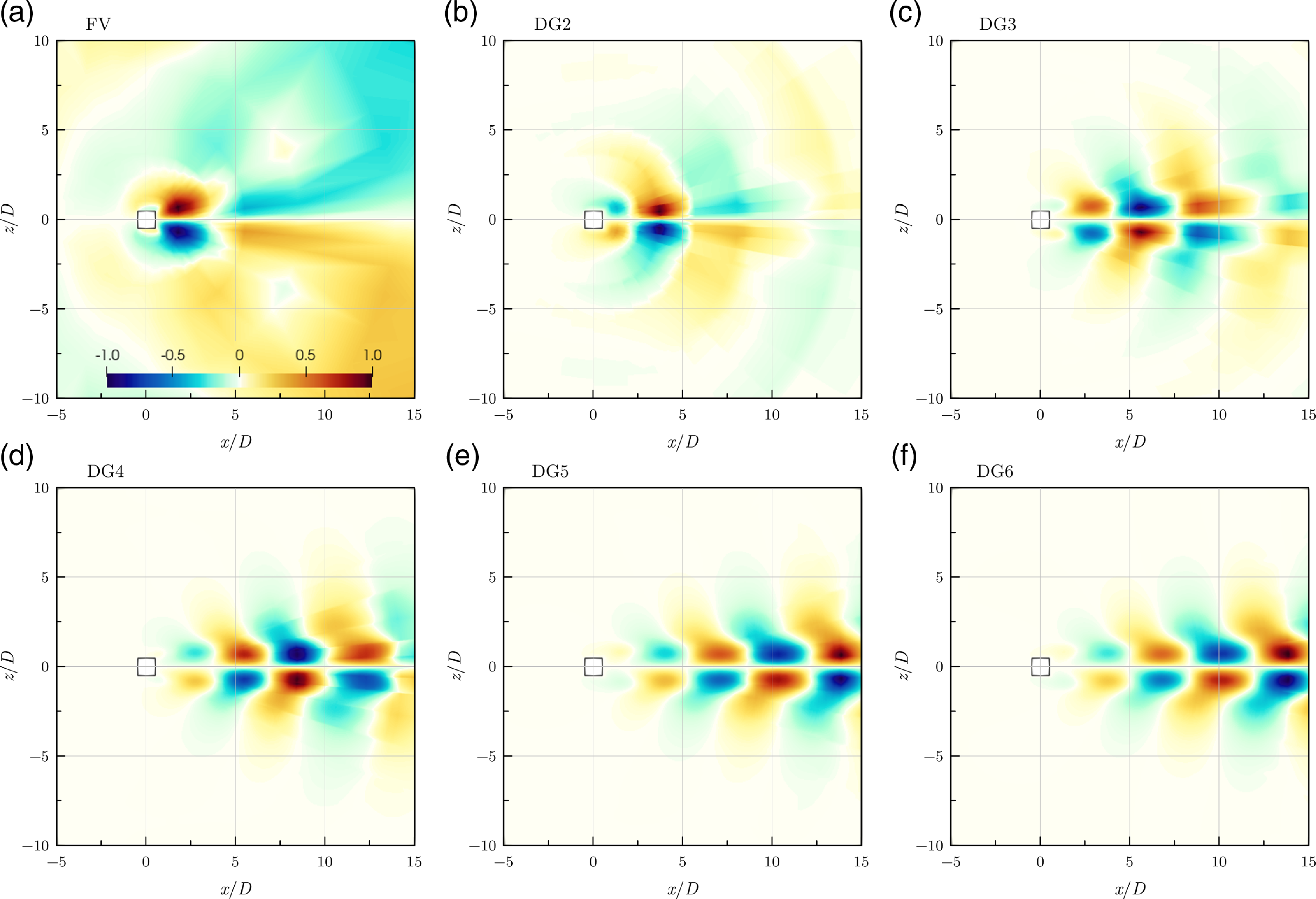
Figure 8. Streamwise momentum component of unstable direct modes computed on grid L0 with CODA.
Table 2. Eigenvalues for laminar flow past square cylinder case using FV schemes
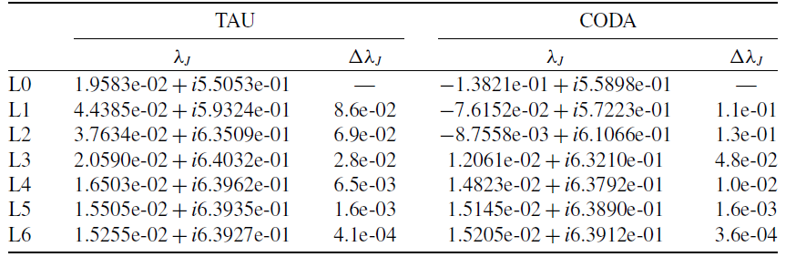
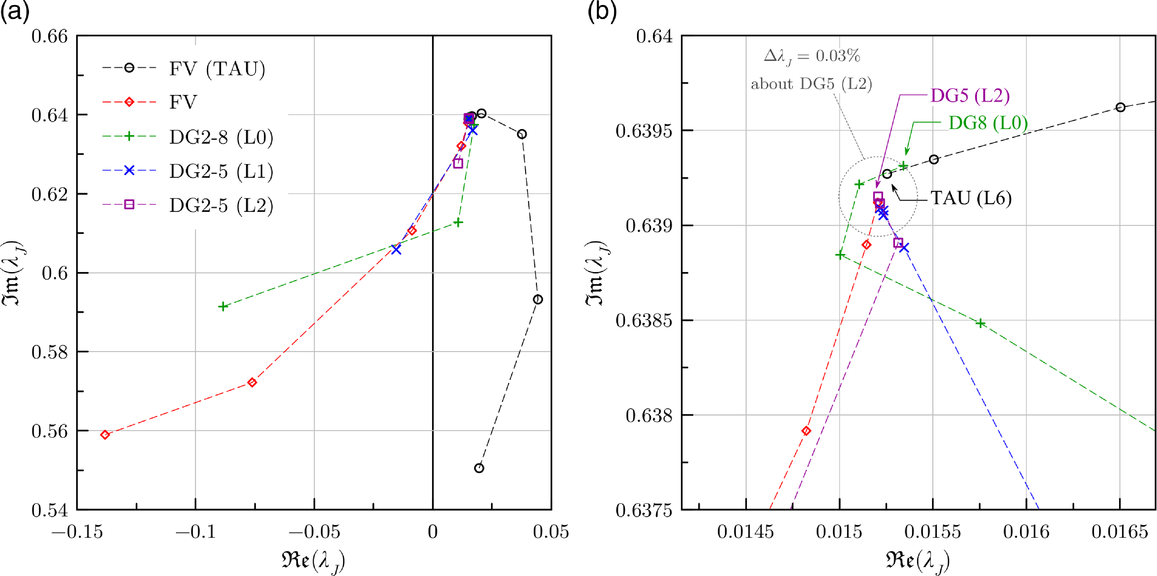
Figure 9. Non-dimensional eigenvalues of the unstable mode for laminar flow past square cylinder case.
The non-dimensional eigenvalues ${\lambda _J}$
for the unstable mode are plotted in Fig. 9. It can be noticed that the FV scheme in CODA does not predict the leading mode as unstable on grids L0 to L2, as evident from the negative real parts of the eigenvalue, but the FV scheme in TAU does so on all grids. With the exception of the second-order DG scheme on grids L0 and L1, all the DG computations are able to capture the unstable mode. The eigenvalues appear to converge with both
${\lambda _J}$
for the unstable mode are plotted in Fig. 9. It can be noticed that the FV scheme in CODA does not predict the leading mode as unstable on grids L0 to L2, as evident from the negative real parts of the eigenvalue, but the FV scheme in TAU does so on all grids. With the exception of the second-order DG scheme on grids L0 and L1, all the DG computations are able to capture the unstable mode. The eigenvalues appear to converge with both $h$
- and
$h$
- and $p$
-refinements. The closeup view in Fig. 9(b), which shows the most converged eigenvalues for each case, suggests that the remaining error, with respect to the true eigenvalue of the continuous equations, for the accomplished refinement levels is less than
$p$
-refinements. The closeup view in Fig. 9(b), which shows the most converged eigenvalues for each case, suggests that the remaining error, with respect to the true eigenvalue of the continuous equations, for the accomplished refinement levels is less than $0.03{\rm{\% }}$
(taking eighth-order DG on grid L0 and fifth-order DG on grid L2 as the worst and best solution, respectively). Since we do not know the true eigenvalue of the continuous equations, we resort to measuring the convergence of the eigenvalues using relative changes in their magnitudes instead. For the FV computations, the relative changes are computed over successive grid levels (
$0.03{\rm{\% }}$
(taking eighth-order DG on grid L0 and fifth-order DG on grid L2 as the worst and best solution, respectively). Since we do not know the true eigenvalue of the continuous equations, we resort to measuring the convergence of the eigenvalues using relative changes in their magnitudes instead. For the FV computations, the relative changes are computed over successive grid levels ( $h$
-refinement), whereas for the DG computations, they are computed over successive orders of the DG scheme (
$h$
-refinement), whereas for the DG computations, they are computed over successive orders of the DG scheme ( $p$
-refinement) for a fixed grid level. Given the eigenvalues on successive refinement levels upon
$p$
-refinement) for a fixed grid level. Given the eigenvalues on successive refinement levels upon $h$
- or
$h$
- or $p$
-refinement, specifically
$p$
-refinement, specifically $\lambda _J^j$
and
$\lambda _J^j$
and $\lambda _J^{j - 1}$
, the relative change is defined as
$\lambda _J^{j - 1}$
, the relative change is defined as
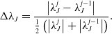 \begin{align}{\rm{\Delta }}{\lambda _J} = \frac{{\left| {\lambda _J^j - \lambda _J^{j - 1}} \right|}}{{\frac{1}{2}\left( \left| {\lambda _J^j}\right| + \left|\lambda _J^{j - 1} \right| \right)}}.\end{align}
Table 3. Eigenvalues for laminar flow past square cylinder case using DG on grid L0
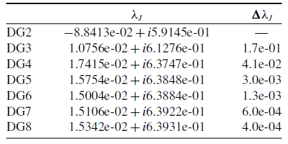
Table 4. Eigenvalues for laminar flow past square cylinder case using DG on grid L1
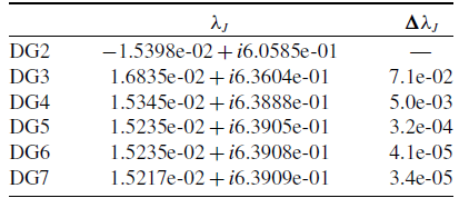
Table 5. Eigenvalues for laminar flow past square cylinder case using DG on grid L2
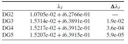
The non-dimensional eigenvalues ${\lambda _J}$
and their relative changes
${\lambda _J}$
and their relative changes ${\rm{\Delta }}{\lambda _J}$
are given in Table 2 for FV computations and in Tables 3–5 for DG computations.
${\rm{\Delta }}{\lambda _J}$
are given in Table 2 for FV computations and in Tables 3–5 for DG computations.
As expected, the value of the relative changes in the eigenvalues decreases with refinement in general. Initially, the eigenvalues computed using CODA’s FV scheme undergo larger changes with grid refinement than those computed using TAU’s FV scheme indicating that the eigenvalues computed on the coarser meshes using the former solver are further away from the exact value than those computed using the latter. Despite the initial slow convergence, FV computations on the finest grids L5 and L6 show similar convergence trends (cf. Table 2). This can also be confirmed in Fig. 9(b) in which the eigenvalues computed on grid L5 using the FV schemes in CODA and TAU are somewhat equidistant from the true value of the continuous equations, which should be in the vicinity of the eigenvalue computed using fifth-order DG scheme on grid L2. It can be seen from Table 3 that a sixth-order DG scheme on grid L0 surpasses this with only 0.13% change in the eigenvalue, while an eighth-order DG scheme on grid L0 achieves similar accuracy as the FV scheme in TAU on grid L6. The convergence of the eigenvalues computed using DG schemes improves on grid L1 with $0.0034{\rm{\% }}$
change for a seventh-order scheme and grid L2 with
$0.0034{\rm{\% }}$
change for a seventh-order scheme and grid L2 with $0.0059{\rm{\% }}$
change for a fifth-order scheme. Finally, the mode computed on grid L3 using third-order DG is almost identical (with a
$0.0059{\rm{\% }}$
change for a fifth-order scheme. Finally, the mode computed on grid L3 using third-order DG is almost identical (with a $0.002{\rm{\% }}$
difference) to that of the fifth-order DG scheme on grid L2.
$0.002{\rm{\% }}$
difference) to that of the fifth-order DG scheme on grid L2.
While the advantages of DG schemes for the non-linear flow problem are often stated in the literature in terms of computational cost, for the herein presented linearised stability analysis it can be said that high-order DG schemes were able to achieve a given level of convergence (measured using ${\rm{\Delta }}{\lambda _J}$
) much faster than the FV scheme. For instance, CODA FV computation on grid L5 and sixth-order DG scheme on grid L0 both achieved the same level of convergence but the computation time for the latter was an order of magnitude lower than the former. However, this is a rather intricate discussion; for instance, convergence can be strongly affected by the condition number of the shift-invert matrix eigenvalue problem.
${\rm{\Delta }}{\lambda _J}$
) much faster than the FV scheme. For instance, CODA FV computation on grid L5 and sixth-order DG scheme on grid L0 both achieved the same level of convergence but the computation time for the latter was an order of magnitude lower than the former. However, this is a rather intricate discussion; for instance, convergence can be strongly affected by the condition number of the shift-invert matrix eigenvalue problem.
5.0 Summary
The Krylov–Schur algorithm for solving large eigenvalue problems has been implemented within the framework of the next-generation flow solver CODA. The implementation was validated using laminar flow past a circular cylinder case for which the eigenvalues and eigenvectors computed using the FV scheme in CODA were shown to agree qualitatively with those computed using the FV scheme in TAU for both the direct and adjoint eigenvalue problems. The case of laminar flow past a square cylinder was used to investigate the possible benefits of using high-order DG schemes over FV scheme for solving the eigenvalue problem. The results presented herein demonstrate that, unlike the FV schemes which require very fine meshes, high-order DG schemes lead to well-converged eigensolutions on coarser meshes at a lower computational cost.
Acknowledgements
The work leading to these results received funding through the UK project Development of Advanced Wing Solutions (DAWS). The DAWS project is supported by the Aerospace Technology Institute (ATI) Programme, a joint government and industry investment to maintain and grow the UK’s competitive position in civil aerospace design and manufacture. The programme, delivered through a partnership between ATI, Department for Business, Energy & Industrial Strategy (BEIS) and Innovate UK, addresses technology, capability and supply chain challenges.
CODA is the computational fluid dynamics (CFD) software being developed as part of a collaboration between the French Aerospace Lab ONERA, the German Aerospace Center (DLR), Airbus, and their European research partners. CODA is jointly owned by ONERA, DLR and Airbus.
We thank the University of Liverpool for computing time on the high-performance computing system. The simulation data that support the findings of this study are available from the authors upon reasonable request.
Competing interests
The author(s) declare none.
Appendix A
Algorithm 1. Krylov–Schur algorithm.
Appendix B
The diagonal elements of the upper-triangular matrix ${S_k}$
need to be reordered using orthogonal similarity transformations prior to the restart. Without loss of generality, let us consider a
${S_k}$
need to be reordered using orthogonal similarity transformations prior to the restart. Without loss of generality, let us consider a $2 \times 2$
upper-triangular matrix
$2 \times 2$
upper-triangular matrix
 \begin{align}{S_2} = \left[ {\begin{array}{c@{\quad}c}a &b\\[5pt] {} & c\end{array}} \right],\end{align}
to which we apply an orthogonal similarity transformation ${S'_{\!\!2}} = U{S_2}{U^H}$
which swaps the diagonal elements
${S'_{\!\!2}} = U{S_2}{U^H}$
which swaps the diagonal elements $a$
and
$a$
and $c$
while keeping
$c$
while keeping ${S'_{\!\!2}}$
upper-triangular. Let us assume that
${S'_{\!\!2}}$
upper-triangular. Let us assume that $a \ne c$
since if
$a \ne c$
since if $a = c$
, no swapping would be needed in the first place. A
$a = c$
, no swapping would be needed in the first place. A $2 \times 2$
orthogonal matrix
$2 \times 2$
orthogonal matrix $U$
can be written as
$U$
can be written as
 \begin{align}U = \left[ {\begin{array}{c@{\quad}c}p & q\\[5pt] {{q^H}}& { - {p^H}}\end{array}} \right],\end{align}
where $p{p^H} + q{q^H} = 1$
. Since we require the bottom-left element of
$p{p^H} + q{q^H} = 1$
. Since we require the bottom-left element of ${S'_{\!\!2}}$
to be zero, we arrive at the condition
${S'_{\!\!2}}$
to be zero, we arrive at the condition
 \begin{align}{q^H}\left( {d{p^H} - b{q^H}} \right) = 0,\end{align}
where $d = c - a$
. Setting
$d = c - a$
. Setting ${q^H} = 0$
satisfies the condition but it leads to the trivial case
${q^H} = 0$
satisfies the condition but it leads to the trivial case $U = I$
which does not swap the diagonal elements. Therefore, the term inside the brackets must vanish and Equation (18) reduces to
$U = I$
which does not swap the diagonal elements. Therefore, the term inside the brackets must vanish and Equation (18) reduces to
 \begin{align}\frac{{{p^H}}}{{{q^H}}} = \frac{b}{d}.\end{align}
Since $a \ne c$
, the denominator on the right-hand side does not vanish. Similarly, since
$a \ne c$
, the denominator on the right-hand side does not vanish. Similarly, since ${q^H} = 0$
is not considered, the denominator on the left-hand side also does not vanish. Multiplying Equation (19) with its complex conjugate and substituting
${q^H} = 0$
is not considered, the denominator on the left-hand side also does not vanish. Multiplying Equation (19) with its complex conjugate and substituting $q{q^H} = 1 - p{p^H}$
leads to
$q{q^H} = 1 - p{p^H}$
leads to
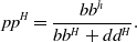 \begin{align}p{p^H} = \frac{{b{b^h}}}{{b{b^H} + d{d^H}}}.\end{align}
We can choose $p$
to be real and positive with a magnitude equal to the square root of the value on the right-hand-side of Equation (20). The value of
$p$
to be real and positive with a magnitude equal to the square root of the value on the right-hand-side of Equation (20). The value of $q$
can be obtained from Equation (19) as
$q$
can be obtained from Equation (19) as $q = p{d^H}/{b^H}$
.
$q = p{d^H}/{b^H}$
.
To prove that the diagonal elements are indeed swapped, let us compute the top-left element of ${S'_{\!\!2}}$
and show that it is equal to
${S'_{\!\!2}}$
and show that it is equal to $c$
;
$c$
;
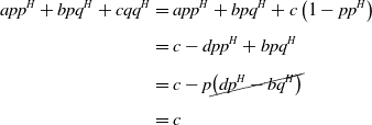
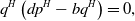
The cancellation in the third line occurs due to Equation (19). A similar computation of the bottom-right element of ${S'_{\!\!2}}$
shows that it is equal to
${S'_{\!\!2}}$
shows that it is equal to $a$
. Alternatively, one can reason that since an orthogonal similarity transformation preserves the eigenvalues and since the eigenvalues of an upper-triangular matrix appear on its diagonal if the top-left element of
$a$
. Alternatively, one can reason that since an orthogonal similarity transformation preserves the eigenvalues and since the eigenvalues of an upper-triangular matrix appear on its diagonal if the top-left element of ${S'_{\!\!2}}$
is
${S'_{\!\!2}}$
is $c$
, the bottom-right element of
$c$
, the bottom-right element of ${S'_{\!\!2}}$
must be
${S'_{\!\!2}}$
must be $a$
.
$a$
.
In the current implementation, the diagonal elements of ${S_k}$
are reordered by repeatedly sweeping down the diagonal and swapping adjacent diagonal elements as needed until no more swaps occur during a sweep. If we wish to swap diagonal elements
${S_k}$
are reordered by repeatedly sweeping down the diagonal and swapping adjacent diagonal elements as needed until no more swaps occur during a sweep. If we wish to swap diagonal elements ${s_j}$
and
${s_j}$
and ${s_{j + 1}}$
, the similarity transformation matrix
${s_{j + 1}}$
, the similarity transformation matrix $V$
can be constructed by replacing the
$V$
can be constructed by replacing the $2 \times 2$
diagonal block of a
$2 \times 2$
diagonal block of a $k \times k$
identity matrix at location
$k \times k$
identity matrix at location $\left( {j,j} \right)$
with the
$\left( {j,j} \right)$
with the $2 \times 2$
orthogonal matrix, specifically
$2 \times 2$
orthogonal matrix, specifically
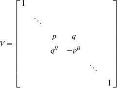 \begin{align}V = \left[ {\begin{array}{c@{\quad}c@{\quad}c@{\quad}c@{\quad}c@{\quad}c}1 & {} & {}& {}& {}& {}\\[5pt] {} & \ddots & {} &{} &{} &{}\\[5pt] {}& {}& p& q& {}& {}\\[5pt] {}& {}& {{q^H}}& { - {p^H}}& {}& {}\\[5pt] {}& {}& {} &{}& \ddots {}\\[5pt] {}& {}& {}& {} &{}& 1\end{array}} \right]\end{align}


 Open access