

Over the past several years, economic inequality has become one of the most discussed topics in social science and social policy. Indeed, no serious discussion of contemporary social and economic life seems complete without a consideration of the growing level of economic inequality that we have seen over the past several decades. In this chapter, I will explore whether, and how, economic inequality – the distribution of income and wealth across social strata – affects the formation and dissolution of families. I write from the perspective of the United States, but I hope my view will be valuable for students of Western Europe and the other overseas English-speaking countries. I will focus on different-sex couples, for whom an historical argument can be assessed. Studies of same-sex couples are underway, and it is not yet clear whether the dynamics are different. I will examine whether economic inequality may be affecting patterns of entry into and exit from cohabitation and marriage, as well as childbearing within or outside marriage. Nevertheless, I will acknowledge that cultural change matters too. Economic conditions are not all powerful. The changes that we have witnessed in family formation would not have happened had the Western world not seen a great shift in attitudes toward marriage and cohabitation over the past half-century.
I have elsewhere referred to these cultural shifts as the deinstitutionalization of marriage (Cherlin Reference Cherlin2004). In retrospect, I think that a more accurate, although less elegant, phrase would have been “the deinstitutionalization of intimate unions.” Marriage itself retains much of its distinctive structure and legal protections, even if it has a less clear set of rules for how spouses are to behave than in the past, but it no longer has a monopoly on intimate unions. A majority of partnerships now begin as cohabiting unions. Cohabiting couples cannot rely on shared understandings and legal statutes to guide their interactions. Rather, they must negotiate how they will act in their relationships. They exhibit a wide variation in commitment. In northern Europe, one commonly finds cohabiting couples who have had long-term stable relationships without ever marrying (Kiernan Reference Kiernan2001), but in the United States, most cohabiting unions lead either to break-ups or to marriage within a few years (Cherlin Reference Cherlin2009). An increasing number of American children are now born into them – one in four at the rates in 2015 (Wu Reference Wu2017). In some cases, the parents may not begin to cohabit until after the woman becomes pregnant (Rackin and Gibson-Davis Reference Rackin and Gibson-Davis2012). Children born to cohabiting couples are exposed to a substantially higher risk of parental union dissolution than are children born to married couples – a relationship common across almost all European countries (DeRose et al. Reference DeRose, Lyons-Amos, Wilcox and Huarcaya2017). Childbearing in cohabiting unions is much more common among Americans without university degrees than among university graduates (Wu Reference Wu2017). A clear social-class line now divides American families at the university-degree level, with graduates much more likely to marry before having a child and less likely to end their marriages. Indeed, it almost seems as though the United States has two family formation systems that are differentiated by the presence or absence of a university degree (Cherlin Reference Cherlin2010).
Economic inequality is relevant for explaining these divergent patterns in partnerships and fertility. A long line of research links marriage formation to labor market opportunities for young men (Becker Reference Becker1991; Oppenheimer Reference Oppenheimer1988; Parsons and Bales Reference Parsons and Bales1955). Men have been, and still are, required to earn a steady income; more recently, it has become desirable, but optional, for women to earn one too – at least among nonpoor couples. Therefore I will focus most of my attention to the changes in the labor market that have affected men. Aggregate-level (e.g., cross-national or cross-state) studies have addressed the consequences of inequality for family-related outcomes, such as the percentages married (Loughran Reference Loughran2002) or divorced (Frank, Levine, and Dijk Reference Frank, Levine and Dijk2014), and for teenage pregnancy and birth rates (Gold et al. Reference Gold, Kawachi, Kennedy, Lynch and Connell2001). My coauthors and I have shown that individuals are more likely to marry before childbearing in places where labor market conditions are better than in places where middle-skilled jobs are scarce (Cherlin, Ribar, and Yasutake Reference Cherlin, Ribar and Yasutake2016). However, statistical studies require specialized knowledge to evaluate, and their mathematical models are almost always subject to limitations. Consequently, nonspecialists often have understandable difficulties evaluating the worth of statistical claims that are made. In this chapter, I would like to present a less technical argument for the proposition that rising income inequality has been an important driver of changes in family. Think of it as a prima facie case – a set of facts that establishes the likelihood that an argument is true, even though it does not prove it. The facts, I hope, will establish the plausibility that income inequality has been an important causal factor. It will also suggest that explanations that reject the importance of income inequality and instead argue that cultural change is the sole driver (e.g., Murray Reference Murray2012) are at best incomplete.
The Dimensions of Income Inequality
Income inequality has several dimensions. Two have received close attention in social commentary. First, much has been written about the growing proportion of income and wealth accruing to people in the highest 1% of the distribution (e.g., Piketty and Saez Reference Piketty and Saez2003). Between the late 1970s and the early 2010s, the amount of income amassed by the top 1% from about 10% to about 20% (Atkinson, Piketty, and Saez Reference Atkinson, Piketty and Saez2011). As dramatic as this rise has been, I would argue that it is not the most important dimension of inequality to think about when studying changes in family structure. Rather, what matters more is a second dimension of inequality: The growing earnings gap between the university-educated (by which I mean individuals with a bachelor’s or university degree or higher) and the nonuniversity-educated. This gap has widened since the 1970s (Autor Reference Autor2014). Prior to that time, manufacturing jobs were more plentiful in the United States. The nation had emerged from World War II as the economic power of the world. In 1948, American factories produced 45% of the world’s industrial output, and the nation’s manufacturing exports accounted for a third of the world total (Cherlin Reference Cherlin2014). The booming economy and a relative shortage of labor (due to the lower birth rates during the Great Depression) created conditions that were favorable to unionization; and labor unions negotiated for higher wages and better fringe benefits (Levy and Temin Reference Levy, Temin, Brown, Eichengreen and Reich2010).
Yet beginning with the oil embargo by the Arab states in the Organization of the Petroleum Exporting Countries in 1973, the long postwar boom subsided. The wages of production workers remained stagnant or declined as manufacturing work moved overseas, where wages were much lower, or was automated, lowering the demand for workers. The proportion of workers who were doing what was commonly called blue-collar work – production workers, craftworkers, fabricators, construction workers, and the like – declined. In contrast, demand for high-skilled professional, managerial, and technical workers remained strong – a development that economists refer to as skill-biased technical change (Autor, Katz, and Kearney Reference Autor, Katz and Kearney2008). It produced a growing earnings gap between middle-skilled workers, who tend to have a secondary-school education, and highly skilled workers, who tended to have a university education. Autor (Reference Autor2014) has estimated that in the period from 1979 to 2012, the rising earnings gap between the typical university-educated household and secondary-school-educated household has cost the latter four times as much in lost income as has the growing concentration of income among the top 1%.
The rising earnings gap has increased inequality by hollowing out the middle of the income distribution, producing what some have called the hourglass economy – a metaphor for the pinched middle (Leonard Reference Leonard2011). Industrial jobs have been the easiest to automate or outsource because they require routine production that can be done by computer or robots or that can be carried out in factories situated far from the place at which the goods they produce will be consumed. In contrast, many low-paying service jobs must be done in person (e.g., waiters, gardeners); and high-paying managerial and technical jobs have remained uncomputerized and performed in the United States. as well. The polarization of low-paying and high-paying jobs, with fewer mid-level jobs in between, creates a higher level of income inequality.
Income Inequality and Family Formation
How then might rising income inequality be associated with changes in family formation? My argument is that the presence of high levels of income inequality is a signal that a weakness exists in the middle of the labor market. That weakness creates the conditions that change family formation. To be sure, income inequality may not inherently be a direct causal force for family change. Perhaps other forms of income inequality in other places at other times might not be as strongly associated with the hollowing out of the middle of the labor market and therefore might have little effect. However, the inequality that we have seen in the United States is connected to the labor market, in that it is harder for a person with a moderate amount of skill – say, a secondary-school diploma and perhaps a few university courses – to get a decent-paying job. In turn, the difficulty of finding middle-skilled jobs depresses rates of marriage and of marital fertility.
The prima facie case for the causal importance of income inequality rests on two basic trends. The first trend is the aforementioned growth since about 1980 of the earnings differential between the university-educated and the less-educated (Autor Reference Autor2014). As I have noted, this gap reflects the relative decline in job opportunities in the middle of the labor market – the kinds of jobs that people without university degrees are qualified for. In addition, among individuals without a university education, the disruption in the middle of the labor market has been sharper for men than for women. Much of the automation and offshoring has occurred among manual occupations that had been seen as men’s work due to their physical, often repetitive, nature at a factory or a construction site. In the American ideal of the working-class family that was socially constructed in the late nineteenth and early twentieth centuries, men were supposed to do jobs that required hard physical labor and to bring home a paycheck for the needs of their wives and children. Sociologist Michèle Lamont refers to this conception of the male role as the “disciplined self” (Lamont Reference Lamont2000) and claims that it has been common among White working-class men in the United States. (Lamont found that the self-sufficient breadwinner image was less common among Blacks.) It is this type of manly work that has been subject to shortages and to wage stagnation. Initially, working-class husbands took pride in keeping their wives out of the labor force, but in the postwar period, women moved into paid employment in clerical and service work – the so-called pink-collar jobs that came to be seen as women’s work. Jobs in this sector of the economy have not been hit as hard by the offshoring and automation of production. Consequently, men and women’s earnings have moved in different directions. Between 1979 and 2007, men’s hourly earnings decreased for all those without university degrees. For women, earnings fell only for those without secondary-school diplomas; all others experienced increases. Alone among male workers, the university graduates experienced an increase; and for women, the largest increases were for university graduates (Autor Reference Autor2010).
The second basic trend consists of the divergent paths that family structure has taken during the same period, according to the educational levels of the adults involved. In the 1950s, marriage was ubiquitous. At all educational levels, almost everyone married, and almost all children were born within marriage (Cherlin Reference Cherlin1992). The central position of marriage in family life began to erode in the 1960s and 1970s. Crucially for my argument, the trends in marriage and childbearing were initially moving in the same direction for adults at all educational levels: Marriage was being postponed, cohabitation was increasing, and divorce rates were rising (Cherlin Reference Cherlin1992). However, since about 1980, the family lives of those with a university degree, whom we may call the highly educated, and those with less education have diverged (McLanahan Reference McLanahan2004). Family life among the highly educated remains focused on marriage as the context for raising children, and although the highly-educated marry at later ages, they ultimately have higher lifetime marriage rates than do those with less education (Aughinbaugh, Robles, and Sun Reference Aughinbaugh, Robles and Sun2013). In addition, the divorce rate for highly educated couples has declined sharply since its peak around 1980 (Stevenson and Wolfers Reference Stevenson and Wolfers2007). Meanwhile, the percentage of births outside marriage among the highly educated has remained low. In contrast, the family lives of people with a secondary-school diploma but not a university degree, whom we may call the moderately educated, have moved away from stable marriage. This group has experienced a surge of births within cohabiting unions. Unlike the typical cohabiting unions in some European countries, these unions tend to be brittle and to lead to disruptions at a high rate (Musick and Michelmore Reference Musick and Michelmore2015). Among moderately educated married couples (those with secondary-school diplomas), there has not been as much decline in divorce as among the highly educated (S. P. Martin Reference Martin2006). Finally, people without secondary-school degrees, whom we may call the least-educated, have continued to have a high proportion of births outside marriage, although there has been less change in their family patterns since 1980.
Consequently, the greatest change in children’s living arrangements since 1980 has occurred among the moderately educated, among whom the proportion of children living with single mothers and cohabiting mothers has increased dramatically. Figure 3.1 shows changes in children’s living arrangements for the thirty-year period from 1980 to 2010. Consider the white-colored bars, which show the percentage of children with highly educated mothers who are living in a single-parent or cohabiting-parent family. It hardly changed during the thirty-year period – rising from 8% to 11%. In other words, there was little or no movement away from marriage-based families for the raising of children. Now look at the dark-gray bars, which show children living with least-educated mothers. They were the most likely to live in single-parent or cohabiting-parent families in all years but after increasing from 1980 to 1990, the rate has held steady.

Figure 3.1 Percentage of children living with single and cohabiting mothers, by mother’s education, 1980–2010.
It is the light-gray bars, which show children living with moderately educated mothers, that portray the greatest changes in family structure. Here we see the substantial growth of the proportion of children living in single-parent or cohabiting-parent families – from 15% to 30%. Thus, it is among the moderately educated, that we see both the greatest change toward nonmarital, unstable living arrangements for having and rearing children and the greatest erosion of labor market opportunities – and we see both trends commencing at roughly the same point in time. It is among the highly educated that we see the opposite pairing of trends: Continued high levels of children living in more stable marriages centered on marriage coincided with a rise in the earnings premium for university graduates. This is the prima facie case for the proposition that rising income inequality has been an important indicator of changes in family formation – a marker for the deterioration of the middle of the labor market, especially for men, and an improvement in the labor market for the university-educated. Those who experienced a deteriorating job market trended toward less stable family environments. Those who experienced an improvement in the job market trended toward stable marriage-based family environments.
Many of the highly educated are living an advantaged family life, with two earners providing an ample household income. It is the flipside of the family troubles experienced by the moderately educated. In fact, a number of European and American researchers are claiming that the relatively stable unions of the highly educated are based on a new marital bargain in which the partners share the tasks of paid work, housework, and child-rearing more equally than in the past (Esping-Andersen Reference Esping-Andersen2009, Reference Esping-Andersen2016; Esping‐Andersen and Billari Reference Esping–Andersen and Billari2015; Goldscheider, Bernhardt, and Lappegård Reference Goldscheider, Bernhardt and Lappegård2015). For these observers, the key driver has been the change in women’s roles and the normative shift it has caused. In the mid-twentieth century, marriage and family life was in a stable equilibrium based on a specialization model in which the wife did the housework and child care and the husband did the waged work. When wives began to move into the labor force, they also began to ask their husbands to do more in the home. The result, it is said, was several decades of disruption and dissension as husbands resisted taking on more of what had been seen as wives’ work and as welfare states were slow to support women wage workers through programs such as child-care assistance. However, these scholars argue that a new egalitarian equilibrium is emerging that is based on the sharing of both market and housework by the partners, who may now be either married or cohabiting, and who rely on expanded state support for two-earner families. Social norms, according to this view, have evolved from a breadwinner/homemaker equilibrium in the 1950s to an egalitarian equilibrium that is emerging now.
However, an important limitation of this argument is that the egalitarian bargain rests on the availability of good labor market opportunities for men and generous family-friendly social welfare benefits for couples, such as child-care assistance and family leave. Although the husband is no longer required to be the sole earner of the family, there is still a widespread norm that a man must have the potential to be a steady earner in order to be considered as a good long-term partner (Killewald Reference Killewald2016). Among the moderately educated and least-educated, it is increasingly difficult for men to demonstrate sufficient potential. Consequently, the emergence of a gender-egalitarian equilibrium of committed, domestic work-sharing couples in long-term relationships is likely to be more common in the privileged, university-educated sectors of Western nations than in the less-advantaged, lower educated sectors.
The Influence of Cultural Change
The main counterargument to the prima facie explanation I have presented is that changes in social norms have driven both the decline in earnings among the nonuniversity graduates and the changes in family structure that occurred over the same time span. To be sure, culture is part of the story. During the Great Depression, job opportunities were scarce and yet there was no increase in the percentage of children who were born outside marriage. The reason is that having an “illegitimate” child, as it was called at the time, was socially unacceptable and stigmatizing. Today nonmarital births are much more acceptable than in the past. Without this greater cultural acceptance of alternatives to marriage, we would not have seen the rise in births to cohabiting couples in the United States. Moreover, the weakening of marriage began in the early 1960s, well before the dramatic rise in inequality occurred (Cherlin Reference Cherlin1992).
In fact, marriage is much less central to Americans’ sense of their adult identity today than it was in the past. In the 2002 wave of the General Social Survey – a biennial survey of American adults that is conducted by the research organization NORC at the University of Chicago – respondents were asked which of several milestones a person had to accomplish in order to be an adult. More than nine out of ten selected markers such as being economically independent, having finished one’s education, and not living in one’s parental home, but only about half agreed that one had to be married to be an adult (Furstenberg et al. Reference Furstenberg, Kennedy, McLoyd, Rumbaut and Settersten2004). In the mid-twentieth century, the first step a young person took into adulthood was to get married. The average age at marriage in the 1950s was about 20 for women and 22 for men (US Census Bureau 2016). Only then did you leave home: 90%–95% of all young people married. Today, marriage’s place in the life course, if it occurs at all, is often at the end of the transition to adulthood (Cherlin Reference Cherlin2004). Other paths to adulthood, including having children prior to marrying, cohabiting, and perhaps never marrying, are common and largely acceptable.
A further cultural counterargument is that an erosion of social norms supporting hard work has caused the declining work rates of men, at least in the United States, and by extension, family instability (Eberstadt Reference Eberstadt2016; Murray Reference Murray2012). Although we have seen changes in men’s and women’s work and family roles, one norm has held constant: Men must be able to provide a steady income in order to be considered good candidates for marriage. Killewald (Reference Killewald2016) found that men who are not employed full-time have an elevated risk of divorce, but that low earnings were not necessarily a risk factor as long as the men worked steadily. Other studies suggest that while a woman might choose to cohabit with a man whose income potential is in doubt, she is unlikely to marry him – and he may agree that he is not ready. In focus groups conducted with cohabiting young adults in Ohio, several couples told the researchers that everything was in place for a wedding except for the finances, and that until they were confident of their finances, they would not marry (Smock, Manning, and Porter Reference Smock, Manning and Porter2005).
It is alarming to some observers, then, that the percentage of prime-age men who are working or looking for work has declined, particularly among men without university degrees. Eberstadt (Reference Eberstadt2016) reported that the percentage of 25–54-year-old men who were employed dropped from 94% in 1948 to 84% in 2015. He cites a number of factors, including the employment problems faced by the growing number of men who have returned to the general population after serving prison sentences, but he suggests that a decreasing motivation to work among certain groups of men may be part of the story. In contrast, university-educated men are working almost as hard as in the past (Jacobs and Gerson 2005). One might think, then, that university graduates prefer to work longer hours more than do less educated men.; however, that is not true.
In fact, the General Social Survey shows that there has been a decline in the desire to work long hours among both secondary-school-educated men and university-educated men. In several of the survey’s biennial waves, respondents were handed a card showing five characteristics of a job and asked to rank them in importance. One characteristic was “Working hours are short, lots of free time.” In the 1973–1984 period, the proportion of men aged 25–44 who rated it as most or second-most important was 13%; in the combined 2006 and 2012 samples, it rose to 28% (Cherlin Reference Cherlin2014). It seems, then, the percentage of men who highly valued short working hours and lots of free time has increased. However, the increase was just as sharp for university graduates as it was for those with a secondary-school diploma but not a university degree. (There was no increase among men without secondary-school diplomas.) So both moderately educated and highly educated men seem to value working short hours more than they used to. Yet only the moderately educated men are actually working less than they used to. On the contrary, Americans working in the professional, technical, and managerial sectors of the labor force tend to work longer hours than their European counterparts (Jacobs and Gerson 2005). The survey results therefore raise this question: If both highly educated men and moderately educated men had a growing preference for shorter hours and more free time, why was only the latter group actually working shorter hours than in the past?
The answer, I would argue, is that employment opportunities and earnings levels for the university-educated men were improving so much that some of these men decided to work longer hours than they preferred: The attraction of the jobs that were available to them – notably higher wages and salaries – more than balanced their attraction to free time. Among moderately educated men in contrast, employment opportunities were not attractive enough to override their growing preference for free time. In other words, whether a man is working depends on both his preferences for work and the opportunities available to him. The decline in men’s labor force participation is rooted in a cultural shift as well as a change in the labor market. Both cultural and labor market factors are necessary to explain the decline.
More generally, this example suggests how intertwined economics and culture are in producing the trends we have seen in family life. Economic sociologists have long argued that economic action is embedded in social institutions (Granovetter Reference Granovetter1985): People make decisions about employment in a cultural milieu. Currently, that milieu may be more favorable toward other activities and leisure than in the past. Some observers might judge that milieu negatively and decry the choices working-age men may make, but cultural forces can be overridden by the opportunity for higher paying, stable work or they can be reinforced through job opportunities that are insecure and lower paying. Cultural forces do not alone determine how young adults will relate to family and work, and nor, it must be said, do economic forces.
One other cultural phenomenon may be contributing to the class differences, not by its transformation but by its stubborn persistence: Ideas about masculinity (Cherlin Reference Cherlin2014). As I noted earlier, working-class men have taken pride in hard physical labor. Meanwhile jobs that involved caring for and serving others came to be associated with women. These caring-work jobs typically pay less than industrial jobs, which may explain some of the reluctance of men to take them, but they also seem to be devalued in status, at least among men, precisely because they are seen as unmanly jobs (England Reference England2005). As a 53-year-old man who had lost several jobs to automation and to factories that moved to other cities, told a reporter for the New York Times, he never considered work in the health sector of the labor market: “I ain’t gonna be a nurse; I don’t have the tolerance for people,” he said. “I don’t want it to sound bad, but I’ve always seen a woman in the position of a nurse or some kind of health care worker. I see it as more of a woman’s touch” (Miller Reference Miller2017). What we might call conventional masculinity – and what the literature sometimes calls “hegemonic masculinity” (Connell Reference Connell1995) – still prescribes that some jobs are men’s jobs and others are for women. The problem is that men’s jobs have been disproportionately affected by the globalization and automation of production. In the meantime, service jobs have opened up, as in the health sector, but men have resisted taking them. Working-class men’s resistance to doing jobs that are not considered manly enough contributes to the difficulties they face in the labor market.
Discussion
The social-class differences in family formation that are apparent today are not unprecedented. Rather, we are seeing, in a sense, a return to the historical complexity of family life (Therborn Reference Therborn2004). That complexity was apparent throughout the early decades of industrialization during the late nineteenth and early twentieth centuries, when there was a great growth of factory jobs. During this period, traditional-skilled jobs in the middle of the labor market, such as those performed by independent craftsmen, yeomen, and apprentices in small shops, were undercut by factory production. Independent shops either collapsed or turn into larger factories. Inequality increased, and as is the case today, the middle of the labor market was hollowed out. Sharp social-class differences in marriage rates were visible; professional, technical, and managerial workers were more likely to marry than were workers with less remunerative jobs (Cherlin Reference Cherlin2014). The prosperous period of stability just after World War II, when almost everyone married, fertility rates were high, and divorce rates were unusually stable (Cherlin Reference Cherlin1992), was the most unusual time in family life since industrialization and should not be taken as an anchor point.
Nevertheless, the complexity of family life we see today is different from the complexity of the past. The high rates of cohabitation and of childbearing outside marriage that are now prevalent were rare during the disruptions of early industrialization. Nor, as I noted, were they present during the disruption of the Great Depression. The culture of family life was different; alternatives to marriage such as cohabitation and single-parent families (other than those due to widowhood) were unacceptable to most people. So if a young adult was not married, he or she probably lived in the parental home or boarded in another family’s home and remained childless. The growth in the number of people who were living alone is largely a post-World War II phenomenon, as the housing stock increased and wages and salaries (and therefore the ability to pay rent) rose (Kobrin Reference Kobrin1976; Ruggles Reference Ruggles1988). The lives that unmarried young adults in the United States led in the past are more similar to family life today in countries such as Italy, where it is common for twenties to live at home, remain childless, and marry in their late twenties and early thirties.
One must also include the growth of a more individualistic, self-development oriented culture in the story of changes in family formation today. This cultural development may be connected to a larger shift among the population of the wealthy countries to what are called post-materialist values (Inglehart Reference Inglehart1997). As societies have become wealthier and have solved the problem of providing basic needs, it is said individuals have come to value self-expression – the development of one’s personality – over survivalist values such as providing food, shelter, and basic financial support. One aspect of self-expression is the examination of whether one’s intimate partnership continues to meet one’s needs. If not, the self-expressive individual will consider ending that partnership and finding a new one that better fits her or his continually developing self. Thus, self-expression is associated with higher rates of union dissolution and re-formation. Post-materialist values also include a decline in traditional religious beliefs; in the West that decline is consistent with a rise in nonmarital partnerships and childbearing outside marriage. Overall, a rise in post-materialist values is consistent with what demographers have called the second demographic transition (van de Kaa Reference Van de Kaa1987; Lesthaeghe and Surkyn Reference Lesthaeghe and Surkyn1988): The period since the 1970s during which cohabitation, nonmarital births, and low fertility have become common in most Western countries. Moreover, during this period, there has been a decline in civic engagement – social ties, attendance at religious services, and participation in local associations – that has been more pronounced among those without university educations (Putnam Reference Putnam2015).
Note, however, that second demographic transition theory does not explain the continued strength of marriage and the decline in divorce rates that have occurred among highly educated Americans in this period. It provides no explanation for a seeming transition back toward a family form characterized by relatively stable marriage, albeit preceded by cohabitation. Highly educated young adults were previously thought to constitute the nontraditional vanguard, providing new models of family life that diffused down the educational ladder. That is not, however, what we have seen; rather, the patterns in the United States suggest a neo-traditional highly educated class and a growth of nontraditional behavior among those with less education. At least in the United States, then, second demographic transition theory cannot provide us with an explanation for the growing divide in family life.
That divide suggests a role for the momentous changes in the economy that have differentially affected the highly educated and the less educated. Nevertheless, one must be careful in attributing social change solely to economic inequality. It has become the go-to explanation for a wide variety of social phenomena. One frequently cited book claims that inequality has caused anxiety and chronic stress that has led to a long list of consequences that include poorer physical health, higher mortality, greater obesity, lower educational attainment, higher teenage birth rates, greater exposure among children to conflict, higher rates of imprisonment, more drug use, less social trust, and less social mobility (Wilkinson and Pickett Reference Wilkinson and Pickett2009). All of this is deduced solely from macro-level correlations at the national or state level. It seems unlikely that any social phenomenon could have effects this broad, and in any case, macro-level correlations do not prove the case. The claims in the literature (as well as in this chapter) must therefore be carefully scrutinized and subject to further research.
This chapter also presents a very US-centric perspective that may be less applicable in Europe. The American social welfare system is well known to be among the least generous in the Western world – it is the archetype of the “liberal” (free-market oriented) welfare state in the classic formulation of Esping-Andersen (Reference Esping-Andersen1990) – and compared to other nations, it provides a larger proportion of its benefits through programs that are contingent on work effort (Garfinkel, Rainwater, and Smeeding Reference Garfinkel, Rainwater and Smeeding2010). Therefore, it does less to support low-income families that do not have steady wage earners than do the welfare systems in other countries. It also provides less support for working parents, in terms of paid family leave or child-care assistance. This lack of support may be one reason why rates of union instability and childbearing among single parents are high in the United States from an international perspective (see Chapter 1). Moreover, the idea that a couple should not marry until they are confident that they will have an adequate steady income (Gibson-Davis, Edin, and McLanahan Reference Gibson-Davis, Edin and McLanahan2005) seems to be stronger in the United States than elsewhere. Perelli-Harris (Reference Perelli-Harris2014) and her colleagues convened focus groups in nine settings in Europe to discuss cohabitation and marriage. They found that the rise of education has not devalued the cultural meaning of marriage; however, they did not hear much discussion of economic uncertainty and its relationship to whether a cohabiting couple should marry.
Nevertheless, the prima facie case that inequality – and more specifically the diverging labor market opportunities for the highly educated and the moderately educated – has driven family formation and dissolution seems strong for the United States. It is not the complete explanation for the great changes in these behaviors that have occurred in the past half-century or so, but it does not need to be. To be sure, had bearing children outside marriage not become acceptable, had cohabitation not become the predominant way that young adults enter into a first union, had survival values persisted over self-expressive values, we would not have seen the same retreat from marriage and marital childbearing; however, had employment opportunities for secondary-school-educated men not deteriorated and had corporations not been able to use the mobility of capital to undermine unionized factories, we would probably not have seen the same retreat either. Culture alone cannot explain the increasingly divergent paths by which the university-educated and the nonuniversity-educated are forming and maintaining families. It seems highly likely that one must take into account the economic changes that have occurred in the increasingly unequal American society.
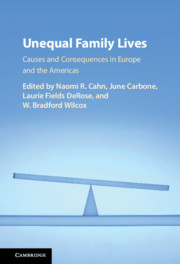
New family formation behaviors have increased nearly everywhere in Europe. Cohabitation, childbearing within cohabitation, divorce, separation, and repartnering have all become more common, even in places where scholars did not think that these behaviors would emerge (see Chapter 1). Recent data from the OECD (2016a) shows that nonmarital fertility, for example, increased dramatically in nearly every country in Europe throughout the 2000s, even across much of southern and Eastern Europe (Figure 4.1). However, European countries still vary widely with respect to the prevalence of new family formation behaviors. For example, in Norway, Sweden, and Denmark, the majority of births occur within cohabitation, while in other countries, such as Italy and Romania, childbearing within cohabitation is still relatively rare (Perelli-Harris et al. Reference Perelli-Harris, Kreyenfeld and Sigle-Rushton2012). Figure 4.1 shows that although nearly every country in Europe experienced increases in nonmarital fertility, the year in which the increases began differs across countries, as does the speed of the increase.
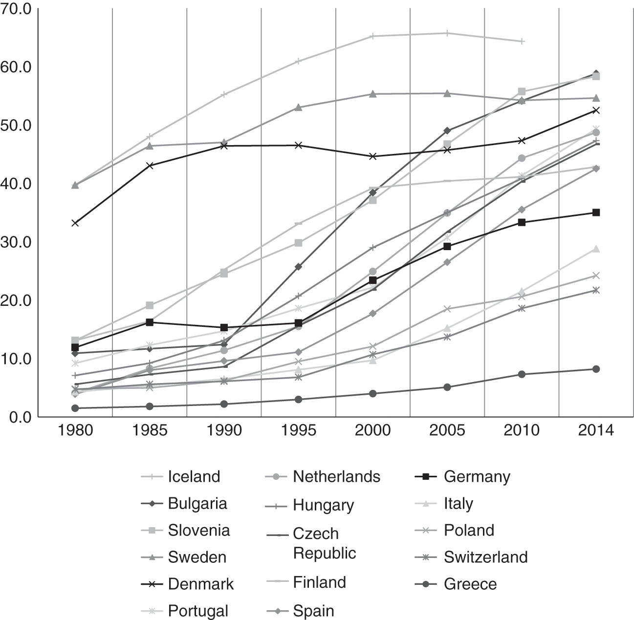
Figure 4.1 Percentage of nonmarital births in selected countries, 1980–2014
The nearly universal increase in new family formation behaviors coupled with the diversity in the timing and rate of increase raises questions about whether the underlying causes are universal, or if the process of development is unique in each context. Several scholars have proposed overarching theories to explain the observed changes, the most well-known of which is the second demographic transition (SDT) (Lesthaeghe Reference Lesthaeghe2010; Van de Kaa Reference Van de Kaa1987). Proponents of SDT theory posit that shifting values, ideational change, and increasing individualization have led individuals to choose unconventional lifestyles and living arrangements, often defying the traditional marital pathway of their parents (Lesthaeghe Reference Lesthaeghe2010). SDT theory also implies that those with higher education were the forerunners of the change, as they challenged patriarchal institutions and focused on the pursuit of self-actualization (Lesthaeghe and Surkyn Reference Lesthaeghe and Surkyn2002).
There is scant evidence, however, that the emergence of new behaviors is due to the pursuit of self-actualization or practiced by the more highly educated. Indeed, recent evidence (as discussed in Chapter 1) indicates that childbearing within cohabitation is associated with lower education (Perelli-Harris et al. Reference Perelli-Harris, Kreyenfeld and Kubisch2010), divorce has increasingly become associated with lower education (Matysiak et al. Reference Matysiak, Styrc and Vignoli2014), and the highly educated are more likely to marry (Isen and Stevenson Reference Isen and Stevenson2010; Kalmijn Reference Kalmijn2013). These studies suggest that new forms of family behaviors are associated with a “pattern of disadvantage.” Although social norms have shifted to become more tolerant of cohabitation and nonmarital childbearing, the less-educated face greater uncertainty and economic constraints, which is reflected in their relationship choices (Perelli-Harris et al. Reference Perelli-Harris, Kreyenfeld and Kubisch2010).
Nonetheless, despite evidence that many aspects of the family are changing across Europe, and some of these new aspects are associated with lower education, a consistent association between family change and social class has not been observed for all behaviors or in all contexts (Mikolai, Perelli-Harris, and Berrington Reference Mikolai, Perelli-Harris and Berrington2014; Perelli-Harris et al. Reference Perelli-Harris, Kreyenfeld and Sigle-Rushton2012). Superficial trends may be masking substantial underlying differences in specific processes and consequences. In fact, research has found that although many aspects of family formation are changing, they might not be converging in the same way or toward a similar standard (Billari and Liefbroer Reference Billari and Liefbroer2010; Sobotka and Toulemon Reference Sobotka and Toulemon2008). Several studies have found that while transitions to adulthood are becoming more complex, heterogeneous, and “destandardized” throughout Europe, trajectories do not appear to be converging on one particular pattern or type of new trajectory (Elzinga and Liefbroer Reference Elzinga and Liefbroer2007; Fokkema and Liefbroer Reference Fokkema and Liefbroer2008; Perelli-Harris and Lyons-Amos Reference Perelli-Harris and Lyons-Amos2015). In addition, while some elements of partnership formation, such as the postponement of marriage, seem to be universally associated with higher education, country context appears to be much more important for predicting partnership trajectories than individual-level educational attainment (Perelli-Harris and Lyons-Amos Reference Perelli-Harris and Lyons-Amos2016). Thus, while some aspects of family formation, such as the postponement of marriage and fertility, seem to be changing on a wide scale, others, such as long-term cohabitation and union dissolution, seem to be dependent on the social, economic, political, religious, and historical contexts that shape family behavior.
In this chapter, I will explore the diversity and similarity of partnership experiences throughout Europe, drawing on recent research and evidence. I will focus on the emergence of cohabitation as a new family form, especially as a context for childbearing. Cohabiting unions are heterogeneous living arrangements, with some couples sliding into temporary partnerships of short duration, others testing their relationship to see if it is suitable for marriage, and still others living in long-term committed unions with no intentions of marriage (Perelli-Harris et al. Reference Perelli-Harris, Mynarska and Berghammer2014). Yet, on average, cohabiting unions are more likely to dissolve, even if they involve children (Galezewska Reference Galezewska2016; Musick and Michelmore Reference Musick and Michelmore2015). Also, as discussed above and in Chapter 1, childbearing within cohabitation is often associated with low education, resulting from a pattern of disadvantage (Perelli-Harris et al. Reference Perelli-Harris, Kreyenfeld and Kubisch2010). Thus, the costs of union dissolution more commonly fall on already disadvantaged individuals, potentially exacerbating inequality.
This chapter will cover findings from a mixed methods project that examined cohabitation and nonmarital childbearing across Europe and the United States from different analytical perspectives.Footnote 1 First, I will describe the spatial variation in nonmarital fertility across Europe to illustrate how patterns of family change may be influenced by political or cultural borders as well as the persistence of the past. Second, I will outline the laws and policies governing cohabitation in nine European countries to demonstrate how welfare states may be ill-equipped to deal with the new realities of more people living outside marriage. Third, I will draw on a large focus group project to describe discourses surrounding cohabitation and marriage in eight European countries to better understand similarities and differences in cultural and social norms. Finally, I will address the potential consequences of new partnership behaviors by summarizing a recent project that examines the health and well-being of cohabiting and married people. This section will discuss whether marriage, versus remaining in cohabitation, provides benefits to adult well-being beyond simply living with a partner. Throughout, I will speculate about why partnership behaviors differ across countries. Taken together, these studies portray a complex picture of family change in Europe today and raise questions about whether the interrelationship between family trajectories and inequality may be mediated by country context.
The Diffusion of New Family Behaviors: Universal Change – Uneven Distribution
One of the best ways to illustrate the diversity of family formation behaviors is with a map (Figure 4.2, Klüsener, Perelli-Harris, and Sánchez Gassen Reference Klüsener, Perelli-Harris and Gassen2013). The variegated landscape of nonmarital fertility can reveal clues into the fundamental reasons why marriage has declined in some countries, while remaining the predominant context for childbearing in others. Figure 4.1 shows the percentage of nonmarital births across Europe in 2007, with the lightest regions indicating that less than 10% of births occur outside marriage and the darkest regions indicating that up to 75% of births occur outside marriage. Note that the diffusion of nonmarital fertility has primarily been driven by the increase in childbearing within cohabiting partnerships, not births outside a union (Perelli-Harris et al. Reference Perelli-Harris, Kreyenfeld and Sigle-Rushton2012). Thus this map portrays a rapid increase in a new and emerging behavior. More recent nonmarital childbearing statistics on the national level (OECD 2016a) suggest that the entire map has become even darker over the past seven years as the percentage of births outside marriage has reached unprecedented highs; however, these statistics are not available on the regional level. The map shown here is important for showing gradations of patterns on the regional level, thus providing insights into the link between spatial variation and the persistence of the past (Klüsener Reference Klüsener2015).

Figure 4.2 Percentage of births outside marriage, 2007
First, notice that the patchwork of high and low regions does not necessarily accord with particular welfare regimes, or even typical geographic areas. Nonmarital fertility is very high in the Nordic countries, with the highest levels in northern Sweden and Iceland, reflecting a long history of female independence and permissiveness of alternative living arrangements (Trost Reference Trost1978). Nonmarital fertility is also high in France, where cohabitation rose rapidly during the 1980s, possibly due to policies which favored single mothers or as a rejection of the Catholic Church and the institution of marriage (Knijn, Martin, and Millar Reference Knijn, Martin and Millar2007). Eastern Germany also stands out as a region with particularly high levels of nonmarital fertility, dating back to the Prussian era (Klüsener and Goldstein Reference Klüsener and Goldstein2014) and increasing during the socialist period through policies favoring single mothers (Klarner Reference Klärner2015), and after the collapse of socialism, by high male unemployment and female labor force participation (Konietzka and Kreyenfeld Reference Konietzka and Kreyenfeld2002). Of the Baltics, Estonia has the highest level of nonmarital fertility, reflecting greater secularization than in Latvia and Lithuania, which have maintained Catholic or traditional social norms favoring marriage (Katus et al. Reference Katus, Põldma, Puur and Sakkeus2008). Bulgaria is another, southern European, country with unexpectedly high levels of nonmarital fertility, possibly due to cultural practices in rural areas or as a response to economic insecurity (Kostova Reference Kostova2007). Other regions also have surprisingly high nonmarital fertility, for example, parts of Austria and southern Portugal, which harken back to norms only permitting marriage upon inheritance of the family farm.
Very low levels of nonmarital fertility are primarily concentrated in southern Europe, for example, in Greece, Albania, and southern Italy. Studies have indicated that Italy has had a “delayed diffusion” of cohabitation, potentially because parents have opposed their children living together without being married (DiGiulio and Rosina Reference Di Giulio and Rosina2007; Vignoli and Salvini Reference Vignoli and Salvini2014). The vast majority of births also continue to occur within marriage in Bosnia and Herzegovina, Croatia, and Serbia, reflecting traditional religious and cultural practices (Klüsener Reference Klüsener2015). In addition, a large swathe of Eastern Europe has very low levels of nonmarital fertility, including parts of eastern Poland, Western Ukraine, and Belarus. Thus, this map and more recent data (OECD 2016a) indicate that some areas appear to be resistant to the changes sweeping across Europe, although some of the very low levels may be due to underreporting (Klüsener Reference Klüsener2015).
When we look closer at the map, we can further see that both political and cultural borders can be very important for delineating the patterns of nonmarital fertility (Klüsener Reference Klüsener2015). In some instances, distinct state borders imply that national policies and legislation can have a strong effect on decisions to marry. For example, the Swiss–French border denotes a sharp distinction between high levels of nonmarital fertility in France and low levels in neighboring Switzerland, despite sharing a similar language and employees who commute daily. The strong distinction in nonmarital fertility is most likely due to strict Swiss policies for unmarried fathers, who were not allowed to pass down their surname if they were not married to the mother of their child. Note, however, that these policies were recently relaxed, and 2014 estimates indicate rapid change with one fifth of all Swiss births outside marriage (OECD 2016a).
In some regions, however, state borders do not define patterns of nonmarital fertility, suggesting that cultural or religious influences are more important. For example, the percentage of nonmarital births is very low across the borders of eastern Poland and Western Ukraine, despite different family policy regimes (Sánchez Gassen and Perelli-Harris Reference Sánchez Gassen and Perelli-Harris2015), indicating that the long history of Catholicism in this area has maintained strong social norms toward marriage. Furthermore, some countries have strong differences within their borders, for example nonmarital childbearing varies considerably from the north of Italy to the tip of the boot. In sum, it is fascinating to stare at the map and recognize that both political and cultural factors may influence such a fundamental demographic phenomenon as the partnership status at birth. Below I investigate these factors in more detail.
Policies and Laws: Universal Rights – Unequal Treatment
Along with complex social and cultural factors, the countries of Europe are defined by a complicated array of policies, laws, and welfare institutions, all of which shape the family and the relationship between couples (Neyer and Andersson Reference Neyer and Andersson2008). Family demographers have long examined how welfare state typologies (Esping-Andersen Reference Esping-Andersen1990) and constellations of family policies influence fertility (e.g., Billingsley and Ferrarini Reference Billingsley and Ferrarini2014; Gauthier Reference Gauthier2007; Thévenon Reference Thévenon2011) and lone parenthood (Brady and Burroway Reference Brady and Burroway2012; Lewis Reference Lewis1997). Here, I will discuss the laws and policies that govern marital and cohabiting relationships. This perspective will provide insights into how legal rights and responsibilities are similar or different across countries, sometimes as a result of underlying economic and welfare state models. It is important to keep in mind that laws and regulations often provide couples with a sense of security and stability, which may influence decisions around partnership formation and marriage. In addition, depending on how they are enacted and enforced, laws and policies may also potentially exacerbate disadvantage and inequality.
Up to the 1970s, marriage was the primary way of organizing family life. European states regulated couples and families primarily through the institution of marriage by providing rights such as joint taxation, widow’s pensions, and inheritance only to married couples (Coontz Reference Coontz2005). In addition, states regulated the relationship between parents and their children, for example, children’s rights to maintenance and inheritance and parents’ rights to child custody and recognition. Until the mid-twentieth century, marriage was the only living arrangement in which childbearing was legitimate, but gradually discrimination against children born outside marriage was abolished and single mothers were granted custody. By the mid-1970s, most European states had also developed legal mechanisms for dissolving a marriage that would regulate the division of assets and financial savings and provide alimony to the weaker party in case of divorce (Perelli-Harris et al. Reference Perelli-Harris, Berrington, Gassen, Galezewska and Holland2017a).
Over the past few decades, many states have started to extend the rights and responsibilities of marriage to couples living in nonmarital relationships (Perelli-Harris and Sánchez Gassen Reference Perelli-Harris and Sánchez Gassen2012). The extent of the legal recognition of cohabitation depends on historical developments, resulting in great variation in the degree of harmonization between cohabitation and marriage across the continent (see Figure 4.3). Generally, countries have taken one of several approaches to recognizing and regulating cohabitation (Sánchez Gassen and Perelli-Harris Reference Sánchez Gassen and Perelli-Harris2015). Some countries, for example, Sweden and Norway, have extended many marital rights and responsibilities to cohabiting couples, especially if they meet certain conditions such as living together for a defined period (e.g., two years) or having children together. Countries such as the Netherlands and France have implemented an opt-in approach, which entitles registered partners (in the Netherlands) or PACS (civil solidarity pacts; in France) to additional rights, such as joint income tax and inheritance, but made it easier for them to separate than divorce. Still other countries, such as England and Spain, have taken a piecemeal approach, with rights extended in some policy domains but not others. As Figure 4.3 shows, these different approaches have resulted in countries falling along a continuum in the degree to which they have harmonized cohabitation and marriage policies, with countries that have adopted registered partnerships and marriage-like arrangements at one end, and countries which favor marriage, such as Switzerland and Germany, at the other (Perelli-Harris and Sánchez Gassen Reference Perelli-Harris and Sánchez Gassen2012).
Figure 4.3 Percentage of policy areas (out of 19) that have addressed cohabitation and harmonized them with marriage in selected European countries
Note: R = registered cohabitation or Pacs; U = unregistered cohabitation.
One policy area that has changed in all countries has been the expansion of the rights of unmarried fathers. Unmarried fathers have the right to establish paternity and attain joint – or sole – custody over their children; however, in all countries they must take additional bureaucratic steps to establish paternity and/or apply for joint custody. Another area which is similar across most countries is the restriction of welfare benefits for cohabiting partners. Generally, unemployment benefits are means-tested and based on households, taking into account the income of all household members (including cohabiting partners). Other policy areas depend on the fundamental relationship between the state, the individual, and the family. Tax systems in Sweden and Norway, for example, are organized around the individual rather than the couple, resulting in similar tax rules for cohabiting and married individuals. Germany and Switzerland, on the other hand, which continue to favor the male breadwinner model, only allow married couples to benefit from tax breaks if one partner earns more than the other.
One of the areas which can have the greatest consequences for the reproduction of inequality is whether cohabitants who separate are protected by the law or have access to family courts. As many studies have shown, cohabiting couples have higher dissolution risks, even when the couple has children together (Galezewska Reference Galezewska2016; Musick and Michelmore Reference Musick and Michelmore2016). Often these couples have lower education and income, putting them at greater risk of falling into poverty (Carlson (this volume); Perelli-Harris et al. Reference Perelli-Harris, Kreyenfeld and Kubisch2010). The lack of legal protection for cohabiting couples can be especially pertinent if one partner (usually the woman) is financially dependent, due to household maintenance and child care, or gender wage differentials. In some countries, such as the UK, the lack of legal regulation may restrict the vulnerable partner’s access to state resources that help to solve property disputes or apply for alimony (The Law Commission 2007). Even though the state may require unmarried fathers to pay child maintenance, the regulations may not be sufficient if the mother does not have access to the courts or the resources to hire a lawyer. In addition, cohabiting partners without children have no legal claim to resources, even if they contributed to the relationship, which could result in a substantial decline in living standards for the vulnerable partner (Sánchez Gassen and Perelli-Harris Reference Sánchez Gassen and Perelli-Harris2015).
Again, protections upon separation depend on whether the state has implemented registered partnerships and the degree to which the state organizes benefits around individuals or families. Registered partners in the Netherlands have many of the same rights as married partners in respect of the division of household goods, the joint home, other assets, and alimony. PACS in France have fewer regulations governing the division of household goods and assets, and no provision for alimony. Sweden and Norway regulate the division of household goods and assets for cohabiting couples, but the tax and transfer system is based on the individual. Most other European countries provide no legal guidance during separation for cohabitants, with the exception of provisos for those separating with children; for example, Germany and Switzerland require separated fathers to pay maintenance to their partners while their children are very young. Overall, this lack of regulation can make it very difficult for vulnerable cohabiting individuals to apply for maintenance or support, and as a result income may fall more after cohabitation dissolution than after divorce.
Nonetheless, it is important to remember that many individuals cohabit precisely because they want to avoid the legal jurisdiction of marriage. They may want to keep their finances and property separate, maintain their independence, and avoid bureaucratic entanglements. Previously married cohabitants may decide to remain outside the law to avoid a costly or time-consuming divorce or protect assets for their children. Given the variety of reasons for cohabiting, it is difficult to know to what extent laws should regulate cohabiting relationships, especially if people are likely to slide into relationships without knowing their responsibilities (Perelli-Harris and Sánchez Gassen Reference Perelli-Harris and Sánchez Gassen2012). In any case, it is important to keep in mind how legal and welfare systems may exacerbate the risk of disadvantage. The legal policies governing cohabitation, marriage, and separation across Europe may have implications for whether states protect vulnerable individuals from slipping further into poverty.
Culture and Religion: Universal Themes – Unique Discourses
As described above, the historical, cultural, and social context is fundamental for shaping attitudes and social norms toward family formation. Social norms are reflected in how people talk about families, and what they say about cohabitation and marriage. They also provide insights into how countries are similar or different from each other. This section draws on a cross-national collaborative project, which used focus group research to compare discourses on cohabitation and marriage in nine European countries (see Perelli-Harris and Bernardi Reference Perelli-Harris and Bernardi2015). Focus group research is not intended to produce representative data, but aims to provide substantive insights into general concepts and a better understanding of how societies view cohabitation. Collaborators conducted 7–8 focus groups in the following cities: Vienna, Austria (Berghammer, Fliegenschnee, and Schmidt Reference Berghammer, Fliegenschnee and Schmidt2014), Florence, Italy (Vignoli and Salvini Reference Vignoli and Salvini2014), Rotterdam, the Netherlands (Hiekel and Keizer Reference Hiekel and Keizer2015), Oslo, Norway (Lappegård and Noack Reference Lappegård and Noack2015), Warsaw, Poland (Mynarska, Baranowska-Rataj, and Matysiak Reference Mynarska, Baranowska-Rataj and Matysiak2014), Moscow, Russia (Isupova Reference Isupova2015), Southampton, United Kingdom (Berrington, Perelli-Harris, and Trevena Reference Berrington, Perelli-Harris and Trevena2015), and Rostock and Lubeck, Germany (Klärner Reference Klärner2015). Each focus group included 8–10 participants, with a total of 588 participants across Europe. The collaborators synthesized the results in an overview paper (Perelli-Harris et al. Reference Perelli-Harris, Mynarska and Berghammer2014) and each team wrote country-specific papers, which were published in 2015 as Special Collection 17 of Demographic Research (entitled Focus on Partnerships). The results of this project are the basis for the discussion below.
The most striking finding from the focus group project was how the discourses in each country described a vivid picture of partnership formation unique to that context. In the countries with the lowest levels of cohabitation, Italy and Poland, focus group participants responded that cohabitation provides a way for couples to test their relationship, but in Poland participants tended to emphasize the unstable nature of cohabitation. In both countries, participants discussed the role of the Catholic Church, but in Italy the emphasis was more toward the tradition of marriage and family, while in Poland it was on religiosity and the heritage of the Church. In Western Germany and Austria, participants took a life-course approach to cohabitation and marriage: Cohabitation is for young adults, who are oriented toward self-fulfillment and freedom, while marriage is for later in the life course, when couples should settle down and be more responsible. Thus, marriage signifies stability, protection, and safety, especially for wives and children.
The discourses in the other countries were also unique. In the Netherlands, a recurring theme was that cohabitation was a response to the increase in divorce. Cohabitation was a way of dealing with possible relationship uncertainty, and marriage was the “complete package,” although registered partnerships or cohabitation contracts could also provide legal security. In the United Kingdom, participants expressed tolerance for alternative living arrangements, but unlike in the other countries, differences between higher and lower educated participants were more apparent. The higher educated tended to think marriage was best, especially for raising children, while the lower educated viewed cohabitation as more normative. In Russia, religion was again expressed in a different way. Orthodox Christians referred to a three-stage theory of relationships: Cohabitation is for the beginning of a relationship, registered official marriage comes soon after, and finally, when the relationship has progressed, a church wedding represents the ultimate commitment. Russian participants also discussed how cohabitation and marriage were linked to the concept of trust, which reflects the general state of a society in which individuals have difficulties trusting each other and institutions (Isupova Reference Isupova2015).
Finally, in some countries, cohabitation was much more prevalent and the focus group participants referred to cohabitation as the normative living arrangement. In Norway, cohabitation and marriage were nearly indistinguishable, especially after childbearing. Nonetheless, marriage was not eschewed altogether, and some still valued it as a symbol of commitment and love. Although marriage is increasingly postponed to later in the life course, often even after having children, it is still seen as a way to celebrate the couple’s relationship. In eastern Germany, on the other hand, marriage held very little symbolic value. The focus of relationships was more on the present rather than whether they would last into the future, and for the most part, participants in eastern Germany thought marriage was irrelevant. Klärner (Reference Klärner2015) speculates that the disinterest in marriage is due to the influence of the former socialist regime, which devalued the institution of marriage, but high levels of nonmarital fertility also have historical roots in the Prussian past (Klüsener and Goldstein Reference Klüsener and Goldstein2014), again suggesting that culture shapes behavior.
Given the unique set of discourses within each country, it is difficult to determine which specific social, economic, or legal factors influenced the responses in each country. Some general patterns emerged, for example, in countries with more similar legal rights, such as Norway, cohabitation was perceived to be mostly similar to marriage, while in countries with fewer protections for cohabitants, such as Poland, focus group participants considered cohabitation to be an unstable relationship. However, the association with legal policies was not clear-cut – for example, discourses in eastern and western Germany differed, even though both regions fall under the same marital law regime. Further, despite the lack of legal differences between de facto partnerships and marriage in Australia, many respondents still valued marriage. These cross-national observations again provide evidence that a complex array of cultural and historical factors shape family behaviors.
Despite the distinct discourses expressed across Europe, however, some common themes emerged, which suggests that cohabitation does share an underlying meaning across countries. First, participants in all countries generally saw cohabitation as a less-committed union than marriage, saying that marriage was the “ultimate commitment,” (United Kingdom), “one hundred percent commitment” (Australia), “higher quality” (Russia), or “more binding and serious” (Austria). Several distinct dimensions of marriage were revealed, for example security and stability, emotional commitment, and the expression of commitment in front of the public, friends, and family. Participants in some countries also discussed fear of commitment, especially among men, and due to the increase in divorce (see also Perelli-Harris et al. Reference Perelli-Harris, Berrington, Gassen, Galezewska and Holland2017a). Although the expression of commitment through marriage was a major theme in most countries, many participants pointed out that other factors, such as owning a house or having children, were just as, if not more, important in signaling commitment. In addition, in nearly every country, a few “ideological cohabitants” argued that cohabiting couples were even more committed than married couples, because they did not need a piece of paper to prove their love. Overall, however, these individuals were in the minority, and cohabitation was seen as a less committed relationship than marriage.
Another theme which emerged throughout the focus groups was the idea that cohabitation is a testing ground allowing couples to “try out” the relationship before marriage. Testing was seen as providing the opportunity for partners to get to know each other and separate if the relationship did not work out. In some countries, participants said that cohabitation was the wise thing to do before marriage (Austria), or even mandatory (Norway), but in all countries cohabitation was recognized as a period when couples could live together as if married but (usually) experience fewer consequences if the relationship dissolved. As a corollary, cohabitation was seen as providing greater freedom than marriage, since it was a more flexible relationship. In some instances this meant that partners have greater independence from each other, for example keeping finances separate, and that they can pursue their own individual self-fulfillment – particularly appealing to women who want to escape the traditional bonds of patriarchy. Some asserted that forming a cohabiting partnership was particularly important after a bad experience with divorce. Others said that the freedom of cohabitation permitted individuals to search for new partners and leave the previous partner if a better one comes along.
The focus group discussions suggested that in most of these European countries, marriage and cohabitation continue to have distinct meanings, with marriage representing a stronger level of commitment and cohabitation a means to cope with the new reality of relationship uncertainty. Yet this uncertainty was not expressed with respect to economic uncertainty, as has often been found in US qualitative research (e.g., Gibson-Davis, Edin, and McLanahan Reference Gibson-Davis, Edin and McLanahan2005; Smock, Manning, and Porter Reference Smock, Manning and Porter2005). Although some European participants did discuss the high costs of a wedding, especially in the United Kingdom, they did not say that couples needed to achieve a certain level of economic stability in order to marry. Of course, the format of focus group research may have discouraged individuals from divulging certain reasons for not marrying, and in-depth interviews with low-income individuals may reveal different narratives, but on the whole, the focus group results suggest that the lack of marriage is not primarily about money, but more about finding a compatible partner. Thus, these focus group findings raise questions about whether cohabitation in Europe is quite different than in America, which appears to be experiencing a more extreme bifurcation of family trajectories by social class (Perelli-Harris and Lyons-Amos Reference Perelli-Harris and Lyons-Amos2016).
Consequences – Does Cohabitation Really Matter for People’s Lives?
While focus group participants often talked about marriage being a more committed and secure relationship, except in eastern Germany and, to some extent, in Norway, it is not clear whether cohabitation and marriage are truly different types of unions, and to what extent this matters for adult well-being. A large body of research has found that married people have better physical and mental health (Hughes and Waite Reference Hughes and Waite2009; Liu and Umberson Reference Liu and Umberson2008; Waite and Gallagher Reference Waite and Gallagher2000), but many of these studies compare the married and unmarried, without focusing on differences between marriage and cohabitation. Studies that do examine differences between partnership types often find mixed results (e.g., Brown Reference Brown2000; Lamb, Lee, and DeMaris Reference Lamb, Lee and DeMaris2003; Musick and Bumpass Reference Musick and Bumpass2012), still leaving open the question of whether marriage provides greater benefits than cohabitation.
On the one hand, certain aspects of cohabitation do seem to universally differ from marriage. For example, research has consistently found that, on average, cohabiting unions are more likely to dissolve than marital unions (Galezewska Reference Galezewska2016), even if they involve children (DeRose et al. Reference DeRose, Lyons-Amos, Wilcox and Huarcaya2017; Musick and Michelmore Reference Musick and Michelmore2016). Women who were cohabiting at the time of their first child also have lower second birth rates compared to married women, unless they marry shortly afterwards (Perelli-Harris Reference Perelli-Harris2014). In addition, certain characteristics are consistently negatively associated with cohabitation, for example subjective well-being (Soons and Kalmijn Reference Soons and Kalmijn2009) and relationship quality (Aarskaug Wiik, Keizer, and Lappegård Reference Wiik, Kenneth and Lappegård2012). Thus, some differences between cohabitation and marriage do indeed seem to be universal across countries.
Nonetheless, it is important to keep in mind that many quantitative studies present average associations that do not reflect the heterogeneity of cohabitation or the potential progression of relationships. As discussed above, cohabitation is an inherently more tenuous type of relationship, and many couples use this period of living together to test their relationships. While some of these couples break up, and some eventually marry, many others will live in long-term unions similar to marriage, but without official recognition. Many of these cohabiting relationships can be nearly identical to marriage, providing similar levels of intimacy, emotional support, care, and social networks, as well as benefiting from shared households and economies of scale. Studies of commitment (Duncan and Philips Reference Duncan, Phillips and Park2008) and the pooling of financial resources (Lyngstad, Noack, and Tufte Reference Lyngstad, Noack and Tufte2010) indicate that over time, couples in cohabiting relationships often make greater investments in their relationships, resulting in smaller differences between cohabitation and marriage. Thus, cohabiting relationships have the potential to be identical to marriage, just without “the piece of paper.”
A second key issue that may account for observed differences by relationship type is selection, which posits that different outcomes are not due to the effects of relationship type per se, but instead, the characteristics of the people who choose to be in that type of partnership. As discussed in Chapter 1, many studies find that cohabitants often come from disadvantaged backgrounds, for example their parents had lower levels of education or income (Aarskaug Wiik Reference Wiik2009; Berrington and Diamond Reference Berrington and Diamond2000; Mooyart and Liefbroer Reference Mooyaart and Liefbroer2016) and might have experienced divorce (Perelli-Harris et al. Reference Perelli-Harris, Berrington, Gassen, Galezewska and Holland2017a). Selection mechanisms often persist into adulthood, for example men who are unemployed or have temporary jobs are more likely to choose cohabitation (Kalmijn Reference Kalmijn2011), and women with lower educational attainment are more likely to give birth in cohabitation than women with higher educational attainment (Perelli-Harris et al. Reference Perelli-Harris, Kreyenfeld and Kubisch2010). Studies using causal modeling techniques to control for individual characteristics demonstrate that the union type itself does not matter for well-being; instead, the characteristics which lead to poor outcomes also lead people to cohabit rather than marry (Musick and Bumpass Reference Musick and Bumpass2012; Perelli-Harris and Styrc Reference Perelli-Harris and Styrc2018). Thus, although further research is needed to ensure a lack of causality, existing studies suggest that marriage does not itself provide benefits over and above cohabitation, given that the union remains intact. This is very important to note, given the common perception that cohabiting couples are less committed than married couples.
Again, however, cultural, social, policy, and economic context may be very important for shaping these interrelationships. Local and national context may attenuate differences between cohabitation and marriage in some countries but not in others. Social and cultural norms may reduce differences between the two relationship types if cohabitation is normalized with few social sanctions, or widen the gap if marriage is given preferential treatment or accorded a special status. We would expect few differences in behavior or outcomes in the Nordic countries, where cohabitation is widespread (Lappegård and Noack Reference Lappegård and Noack2015), but we would expect substantial differences in the United States where marriage tends to be accorded a higher social status (Cherlin Reference Cherlin2014).
The legal and welfare state system may also reduce or exacerbate differences. Legal regimes which recognize cohabitation as an alternative to marriage may provide protections that produce a stabilizing effect for all couples, thereby reducing differences in well-being. On the other hand, systems which privilege marriage – for example, with tax incentives promoting a marital breadwinner model – may result in greater benefits to well-being for marriage than cohabitation. Welfare states that provide benefits only to low-income single mothers may also discourage marriage, and even cohabitation, if benefits depend on the income of all adult household members (Michelmore Reference Michelmore2016). Finally, selection effects can differ across countries, with cohabitation primarily practiced by disadvantaged groups in some countries, or practiced by all strata in others.
Given that countries differ by social, legal, economic and selection effect context, the different meanings of cohabitation may result in differential outcomes across countries. To test this hypothesis, I led a project to examine the consequences of new family arrangements in settings representing different welfare regimes and cultural contexts: Australia, Norway, Germany, the United Kingdom, and the United States. The team systematically analyzed a range of partnership and childbearing behaviors, with a specific focus on outcomes in mid-life – around ages 40–50, depending on the survey – after the period of early adulthood relationship “churning” and most childbearing. The outcomes included mental well-being (Perelli-Harris and Styrc Reference Perelli-Harris and Styrc2018), health (Perelli-Harris et al. Reference Perelli-Harris, Styrc and Addo2017b; Sassler et al. Reference Sassler, Addo and Lappegård2016), life satisfaction (Hoherz et al. Reference Hoherz, Perelli-Harris, Styrc, Lappegård and Evans2017), and wage differentials (Addo et al. Reference Addo, Perelli-Harris, Hoherz, Lappegård and Sassler2017). The team used a variety of retrospective and longitudinal studies, and one of the key concerns of the project was to address selection, which could explain the positive relationship between marriage and outcomes but differ across countries. We used a variety of methods, but primarily propensity score matching or propensity weighted regression, which allowed us to test whether those who did not marry would have been better off if they did marry.
Figure 4.4 shows the mean values and confidence intervals for three outcomes: Self-rated health, life satisfaction, and hourly wage in the local currency. The confidence intervals in bold indicate that the modeling approaches described above were unable to eliminate significant differences between married and cohabiting men and women. The results immediately confirm our main hypothesis: The benefits of marriage relative to cohabitation differ across countries, suggesting that context can shape the meanings and consequences of different partnership types. Before including controls, the confidence intervals indicate that married people have significantly better outcomes in the United Kingdom and United States with respect to self-rated health and hourly wages, and in the United Kingdom with respect to life satisfaction (the United States was not included in the life satisfaction study, and Australia was not included in the wage study). Differences in outcomes by relationship type were not as pronounced in Australia, Norway, and Germany, although cohabiting men in Norway did have significantly different wages from married men, and cohabiting men in Australia and women in Norway had significantly different mean life satisfaction from married individuals.

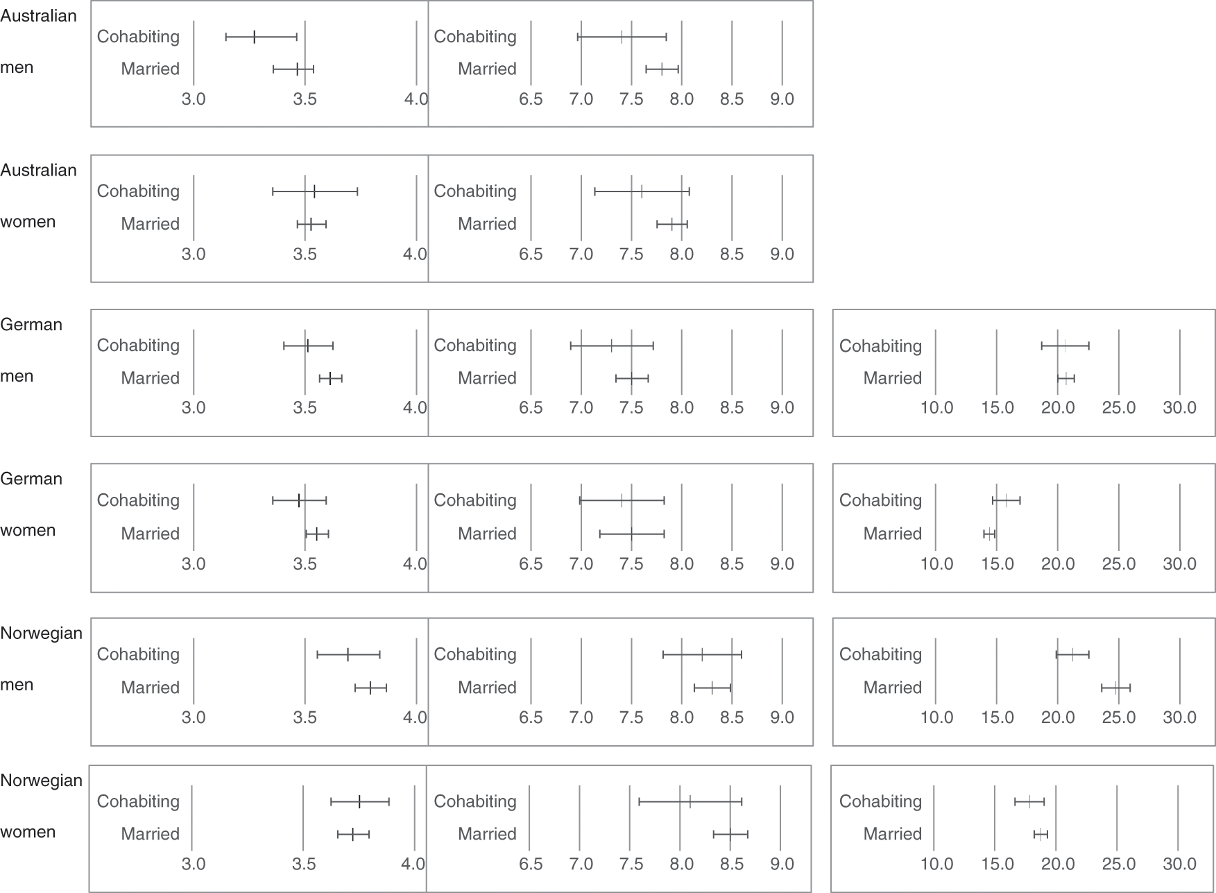
Figure 4.4 Mean values and confidence intervals for outcome variables in selected countries
Once we controlled for different aspects of the union, for example union duration and prior union dissolution, the differences between marriage and cohabitation in health, life satisfaction, and wages were reduced substantially in most studies. This finding suggests that one of the reasons we see differences between cohabitation and marriage is because cohabiting unions are often a testing ground and more likely to dissolve, or they are more commonly chosen as a second union. Cohabiting unions are also less likely to have children together, and controlling for children eliminated many of the differences between cohabitation and marriage. However, one of the main reasons for differences between cohabitation and marriage in mid-life is due to selection mechanisms from childhood, such as parental SES and divorce. After including these indicators in our models, differences by partnership type were reduced substantially and eliminated in the United States. However, some puzzling exceptions remained after including controls: British cohabiting men continued to have worse self-rated health than married men, and both British men and women who were cohabiting continued to have worse life satisfaction than their married counterparts. British married women continued to have slightly higher wages than British cohabiting women. Nonetheless, despite including a large battery of control variables, we suspect that other forms of selection still might account for any effects. Overall, the results suggest that taking into account the heterogeneity of cohabiting unions (as measured by union duration and having children together) as well as selection mechanisms from childhood can explain most of the marital benefits to well-being, but country context, such as welfare state regime and social norms, also matters. Thus, it is important to keep these factors in mind when assessing the extent to which the emergence of cohabitation itself is detrimental to adult well-being; in many places, simply forming a lasting partnership seems to be most important.
Conclusion
Throughout this chapter, I have grappled with the idea that some processes of social change are universal and others are still shaped and reinforced by country-specific factors. I have primarily focused on one of the greatest new developments in the family over the past few decades – the emergence of cohabitation – which has challenged conventional expectations that individuals enter into a lifelong union recognized by law and society. Many people have been alarmed by this development, especially because studies indicate that rates of union dissolution are higher among cohabitants than married couples, and that cohabitation is often associated with disadvantage or low subjective well-being. However, many studies mask the heterogeneity in cohabiting couples and therefore make assumptions about cohabitation that may not be accurate, especially across different settings. In this conclusion, I will briefly summarize and reflect on the different types of heterogeneity which are important to think about when considering whether emerging forms of family behavior, such as cohabitation and nonmarital fertility, are producing and reproducing disadvantage, or whether the behaviors are simply a product of new social realities and shifting norms.
First, countries are diverse and reflect heterogeneous patterns of change. Some countries have experienced rapid increases in cohabitation and nonmarital fertility, while others have not. The variation in family behaviors across Europe reflects different cultural, social, political and economic path dependencies, and the explanations for change cannot be boiled down to one factor. The nonmarital childbearing maps show that sometimes laws and policies can produce differences in behaviors that are distinctly demarcated at state borders, while sometimes religious and cultural factors create pockets of behaviors that stretch across state borders. The discourses from the focus groups also suggest that culture and religion continue to echo in social norms today. Thus, while some general explanations may be similar, we cannot assume that all countries are experiencing the same changes in the family for the same underlying reasons, or that the family change will have the same consequences in the long run.
Second, within countries, we see heterogeneous responses to social change, with some strata of society experiencing increases in new behaviors and other strata not. On the one hand, cohabitation and increases in nonmarital fertility are occurring across all educational levels in most European countries (Perelli-Harris et al. Reference Perelli-Harris, Kreyenfeld and Kubisch2010). In many countries, cohabitation is becoming a normative way to start a relationship, regardless of educational level, and as a way to test that the relationship is strong enough for marriage. Yet transitions to marriage after the relationship is formed, especially before and after the birth of the first child, may be particularly important for producing inequalities. Across Europe, higher educated individuals are more likely to marry before a birth (Mikolai et al. 2016), and lower educated individuals are more likely to separate after a birth (Musick and Michelmore Reference Musick and Michelmore2016). These findings suggest that different groups may be responding in different ways to new behaviors, potentially leading to “diverging destinies” between the most and least educated (McLanahan Reference McLanahan2004). Thus, social change can influence different groups of people in different ways, and it is important to continue to recognize these heterogeneous responses.
Third, the meanings of cohabitation and marriage can change across the life course, and even throughout relationships. Individuals’ values and ideas undergo a process of development as they age and transition throughout different life stages, and this may result in shifting perceptions of cohabitation and marriage as they grow older. As the Austrian focus groups highlighted, people often think that cohabitation is ideal when individuals are young and free, but marriage is best when individuals are more mature and ready to take on more responsibilities, for example childbearing. This evolution of the importance of marriage may especially be embedded in cultures that perceive marriage to signify stability and security. On the other hand, the purpose and meaning of cohabitation may change as relationships progress. At the beginning of a relationship, cohabitation may be a desirable alternative to living apart and a testing ground to see if the relationship is secure, but as the partners become more committed, sharing a home and investing in a long-term relationship may be just as significant as an official marriage certificate. Thus, both cohabitation and marriage are imbued with multiple meanings that can change across multidimensional life courses linked to other life domains (Perelli-Harris and Bernardi Reference Perelli-Harris and Bernardi2015).
To reiterate, these different types of heterogeneity are essential to keep in mind when considering the association between partnership formation and inequality. The great complexity across settings, couples, and individuals creates challenges for understanding how family change is exacerbating or reinforcing inequalities. While some studies have begun to investigate to what extent family structure is responsible (or not) for increasing inequality (Bernardi and Boertien Reference Bernardi and Boertien2017a; Härkönen Reference Juho, Nieuwenhuis and Maldonado2018), far more research is needed to understand these complex relationships, especially in different contexts.
Introduction
Over the past two generations, America has experienced an extraordinary – and yet somehow, also widely overlooked – collapse of work among its men. In the half-century between 1965 and 2015, work rates for the American male ratcheted relentlessly downward, and an ominous migration gathered force: A “flight from work,” in which ever greater numbers of working-age men exited the labor force altogether. America is now home to a vast “idle army” of jobless men no longer looking for work – as of 2015, over 7 million alone between ages 25 and 55, the traditional prime of working life.
To be sure, the decline of work in America is no longer entirely delimited to men. After decades of postwar increase, the work rates and labor force participation rates for prime-age American women have likewise been falling since roughly the beginning of the new century. But the decline of work for American men is a much longer-term trend, and also one of much larger absolute dimensions – and it is that problem, rather than the similarly troubling decline of work for women, that is the subject of this chapter.
The general decline of work for adult men, and the dramatic, continuing expansion of a class of nonworking males (including those both ostensibly able-bodied and in the prime of life) constitutes a fundamentally new and unfamiliar sort of problem for America. It is a problem with manifold and far-reaching economic, social, and perhaps even political implications.
The implications for the state of American families are immediate and inescapable. Lest it otherwise go unsaid, these “prime working ages” in which the present male work crisis is concentrated overlap significantly with the conventional life course ages for family formation, parenting, and child-rearing for the contemporary American man.
As it happens, the long-term decline of work for prime-age men in modern America has coincided with the long-term decline of the married two-parent family structure. The correspondence and interaction of these two great sea changes in daily life for contemporary Americans is a question of obvious importance.
In the following pages, I will attempt to cast some light on the outlines of this important relationship. My exposition is intended only to be exploratory in nature: I recognize there are deep and vital questions my method and approach cannot answer, or even adequately address. It is thus my hope that this introduction will be followed by more detailed investigation into the complex dynamics in play here.
In this chapter I will: (1) present a broad quantitative overview of the ongoing decline of work for American men, and especially men 25–54 years of age, placed in both an historical and international perspective; (2) offer a corresponding quantitative overview of the attendant changes in the sociodemographic profile of prime working-age American men over this same period; (3) decompose arithmetically contributions to declining long-term work rates and labor force participation rates by major sociodemographic factors, including family structure; and (4) conclude with a discussion of what the evidence indicates, what it may suggest, and directions for further research.
Work Rates and Labor Force Participation Rates for US Men in the Postwar Era
One of the major and defining, if not necessarily widely heralded, social changes in postwar America has been the secular decline in employment-to-population ratios (also known as “work rates”) for men. Work rates for American men have been falling for most of the postwar era.
The US government did not begin releasing continuous monthly data on the American employment situation until after World War II. (We do this today, as we have since late 1947, through the Current Population Survey (or CPS), which is maintained by the US Census Bureau and used by the Bureau of Labor Statistics (or BLS) to gauge employment conditions for the adult civilian noninstitutionalized population.) By any broad measure we choose, the US employment-to-population rates for civilian noninstitutionalized men in 2015 and 2016 were very close to their lowest levels on record – and far lower than levels in earlier postwar decades (see Figure 5.1).

Figure 5.1 Employment-to-population ratio, US males, selected age groups: 1948–2016 (seasonally adjusted)
Between the early 1950s and 2016 – between Eisenhower’s America and Obama’s America – the nation’s work rate for adult men (those 20 years of age and older) relentlessly ratcheted downward. Very broadly speaking, this downward trajectory tracked with the business cycle: With each new recession, male work rates typically hit a new low – and typically failed to snap back to prerecession levels over the course of the subsequent recovery. We tend to think of the Great Recession of 2008/09 as the “epic” event in postwar labor markets, and of course the devastation that it wrought is incontestable. What is not generally appreciated, however, is that the drop in male work rates since the Great Recession accounts for less than a quarter of the total long-term downward spiral of 20+ employment-to-population ratios for American men in the postwar era. Three quarters of that slide took place before the crash of 2008.
Between 1948 and 2015, the work rate for American men 20 and older (all postwar employment data are for the civilian noninstitutionalized population) fell from 85.8% to 68.1% – or by almost 18 percentage points. Put another way, between 1948 and 2015, the proportion of American men 20 and older without paid work of any sort more than doubled – from about 14% to almost 32% (see Figure 5.2). This work rate for adult men in 2015 was only a little over a percentage point higher than the 2010 level (its all-time low, at least to date). It rose just a bit more in 2016, from 68.1% to 68.5%. (It registered 68.7% in July 2017, the latest reading available at this writing.) Despite purportedly “near full employment” conditions, at least according to much of the received wisdom currently circulating in business and policy circles, the work rate for the US male 20+ group was fully one fifth lower in mid-2017 than it had been in 1948, almost seventy years earlier.

Figure 5.2 Percentage of civilian noninstitutionalized prime-age (25–54) males without paid employment: USA 1948–2017 (seasonally adjusted)
Of course the 20+ work rate measure includes men 65 and older (i.e., those of classical retirement age), but when I exclude the 65+ population and look instead at men 20–64 years of age, work rates reportedly trace a long march downward here as well – from 90.8% in 1948 to 78.4% in 2015. The 20–64-year-old male work rate in 2015 was thus nearly twelve and a half percentage points below the 1948 level, meaning work rates in America for men in this “classical” working-age group were only about six sevenths as high in 2015 as they had been in the early postwar era. In 2015, the fraction of US men aged 20–64 not at work was 21.6% – 2.3 times higher than it had been in 1948 – and the situation was only very slightly better in 2016 and mid-2017, when the proportion of men 20–64 years of age without any paid work at all was reportedly 21% and 20.7%, respectively.
Note that the impact on recorded work rates from changes in the population composition within the male 20–64 age group was altogether negligible, accounting for less than one hundredth of the intervening twelve or more percentage point decline for the 1967–2015 period (Eberstadt Reference Eberstadt2016). Population structure effects likewise had virtually no effect on work rate trends for prime working-age men – the 25–54-year-old cohort, whose changing fortunes are the focus of this chapter.
Prime working-age men are a critical demographic cohort for reasons both economic and social. They comprise the backbone of the male workforce, currently accounting for roughly two thirds of the 20+ men in the US workforce today, and close to three quarters of adult US men with paying jobs (Eberstadt Reference Eberstadt2016) (see Table 5.1). They are also the group in which labor force participation tends to be highest, due to health and life cycle considerations, and of course, they are also the group arguably most central to family formation and the raising of children, not only in contemporary America.
Table 5.1 US male employment-to-population ratios: 2015 vs. selected depression years
| Year and source | Employment-to-population ratio, males aged 20–64 (percentage of civilian noninstitutionalized population) | Employment-to-population ratio, males aged 25–54 (percentage of civilian noninstitutionalized population) |
|---|---|---|
| 2015 (BLS) | 78.4 | 84.4 |
| 1940 (Census) | 81.3 | 86.4 |
| 1930 (Census) | 88.2* | 91.2*^ |
Notes: *= calculated for total enumerated population, not civilian noninstitutionalized population
^= 25–44 population – corresponding male 25/44 work ratio for 2015 would be 85.3 for civilian noninstitutionalized population alone
Between 1948 and 2015, for the male 25–54 age group, work rates for prime-age US males sank almost 10 percentage points, from 94.1% to 84.4% (see Figure 5.1). Since 2016 these have improved, the rate was 85.0% for 2016, and registered 85.5% in July 2017. One may say that prime-age male work rates have recovered appreciably since their nadir in the wake of the Great Recession, when they hit 80.6% in the fourth quarter of 2009. Even so, at the time of writing, prime-age male work rates are on a par with the lowest-ever BLS readings before the 2008 crash (i.e., from the depths of the deep recession in the early 1980s).
The drop in the work rate of prime-age US men did not actually commence until roughly two decades after the end of World War II. In 1948, the work rate for this cohort was 94.1% – exactly the same rate recorded in 1965. (Between 1948 and 1965, the entirety of the decline in work rates for adult men – for those 20–64 years of age as well as those 20 and older – was due to falling work rates for the cohorts 55 years of age and above.Footnote 1) Roughly speaking, the long-term decline in prime-age male work rate did not start until around 1965. Therefore I shall use 1965 and 2015 as the end points for much of my analysis in this chapter, as that timeframe neatly offers us a half-century of long-term data on changes in prime-age male work rates and their correlates.
As Figure 5.2 illustrates, the percentage of prime-age men without paid work rose fitfully but inexorably from the 1960s to the present. In the 1960s, the average monthly fraction of prime-age men was 6.3% – not appreciably different from the 6.2% of the 1950s. That mean monthly level has risen markedly in every successive decade since the 1960s. For the decade that commenced in 2010, the monthly average to date works out to an astonishing 16.9% – well over two and a half times the mean monthly level from the 1960s. Naturally, this decadal average is affected by the truly awful employment trends in the immediate wake of the Great Recession. In 2010, a monthly average of 19% of all prime-age males had no paid work of any sort. Yet today’s “new normal” should still give pause. In 2015, the corresponding proportion was 15.7%; in 2016 – that is to say, seven years after the end of the Great Recession – it was still 15.0%; and for the first quarter of 2017, it was slightly over 15%. This range appears to be the “new normal” for America today: An employment pattern where at any given moment between one in six and one in seven prime-age men is not engaged in paid work.
This “new normal” for US male nonwork may be instructively compared to work rates for American men during the Great Depression (see Table 5.1). As we can see, work rates for both men 20–64 years of age and those of prime working age were lower in 2015 than in either 1930 or 1940; the same would be true for male work rates in 2016 and early 2017 if these were added to the table. Contraposition of today’s rates and those from the year 1940 is most meaningful. For one thing, employment data in the 1940 census was for the first time recorded in a manner directly comparable with our postwar jobs data; for another, America’s unemployment rates in 1940 are extremely high, pushing 15% on a nationwide basis – sharply higher than in 1930, when the Depression was just getting underway. Even so, measured work rates for prime-age men were 2 percentage points lower in 2015 than in 1940. Thus, it is empirically accurate to describe the current work crisis for American men as a Depression-scale problem.
The critical difference between the joblessness situation for men in 1940 and 2015, however, concerns the shifting balance between unemployment and economic inactivity. In 1940, the overwhelming majority of the men without jobs were looking for one: That is to say, they were unemployed in the classic definition of that term. Only a relatively small number of the men without jobs were economically inactive: That is to say, not in the labor force, neither working nor looking for work. The situation is reversed today: As of 2015, for every prime-age male formally unemployed, there were three neither working nor looking for work (see Figure 5.3). Modern America’s job problem for prime-age men has principally been a long-term exodus from the labor market, a flight that started in the mid-1960s and as yet shows no sign of stopping. Nonworking (or NILF, not-in-labor-force) men are the very fastest growing component of the civilian noninstitutionalized prime-age male population in America, increasing at over three times the tempo of the overall cohort for fully half a century between 1965 and 2015. The decline in labor force participation rates (or LFPRs, the ratio of persons in the workforce to total population) between 1965 and 2015 amounted to 8.4 percentage points (96.7% vs. 88.3%), while the overall decline in work rates for that same period came to 9.7 percentage points (94.1% vs. 84.4%). This means the retreat from the labor force accounted for nearly seven eighths of the fall in prime-age male work rates in America over that half-century, and unlike withdrawal from the labor force at older ages, mass withdrawal from the workforce in the prime of life cannot plausibly be attributed to retirement.
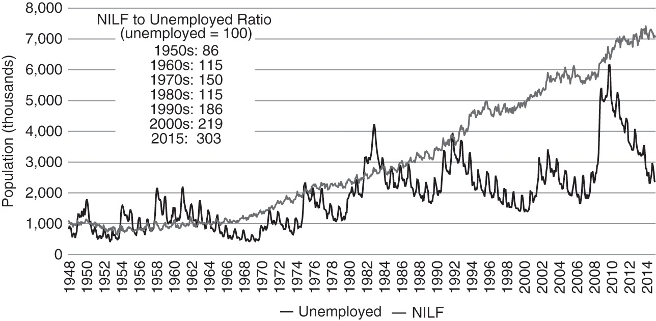
Figure 5.3 Males (25–54) unemployed vs. not in labor force: USA January 1948–May 2016 (seasonally unadjusted)
The postwar prime-age male flight from work has been more extreme in America than in almost any other economically advanced democracy. This is apparent when I compare prime working-age LFPRs for the United States with the corresponding patterns traced out in other “traditional” members of the OECD (or Organisation for Economic Co-operation and Development, the de facto club of affluent aid-giving Western democracies) (see Figure 5.4). This grouping includes Japan, Canada, Australia, New Zealand, and eighteen Western European nations as well as the United States: Twenty-three countries in total. Today, America is at the bottom of all these states in prime-age male labor force participation – twenty-second out of twenty-three, underperformed only by Italy. This troubling state of affairs is also puzzling in a number of respects. For the decline in US prime-age male LFPRs is more severe than in countries beset by “lost decades” of economic growth (e.g., Japan), or those burdened with notoriously dirigiste labor market regulations and hypertrophied welfare states (e.g., France), or even those seemingly enmeshed in perennial debt-and-austerity crises (e.g., contemporary Greece). Why male workforce participation rate performance should be poorer in the United States than in any and all of these comparator states is an important but seldom-examined question.

Sociodemographic Change and the Decline of Prime-Age Male LFPRs, 1965–2015
The sea change in employment patterns for prime working-age men that took place over the years between 1965 and 2015 coincided with a sea change in their sociodemographic profiles. The population profile for American men aged 25–54 in 2015 differed markedly from half a century earlier in a number of respects. Important characteristics that registered major changes over this period included (but were not limited to): Ethnicity, educational attainment, family structure, and nativity (that is to say, whether one was native-born- or foreign-born). In this section, I examine the dimensions of some of these broad sociodemographic shifts within the overall composition of the US prime-age male population, and how these shifts related to both the overall decline of work for prime-age men and the closely related increase in the number of such men who have left the workforce altogether. (As already mentioned, the reference population under consideration here is prime-age men in the “civilian noninstitutionalized population,” per CPS/BLS survey coverage.)
The availability of data series for my examination below does not always nicely match my designated 1965–2015 time frame. Over the decades under consideration, the CPS, from which the BLS’ monthly employment report is derived, gradually extended its scope and asked more detailed and nuanced questions about the nation’s sociodemographic profile. Often, these new questions signified official recognition of the importance of changes already well underway. Thus, in 1965, CPS already provided detailed information on educational attainment for the US population, but its breakdown of data by ethnicity or “race” was still rather rudimentary. It was not until 1971 that it was possible for respondents to identify as themselves as Hispanic, and it took over another two decades before it was possible to do so for Asians, much less multiracial. By the same token, CPS did not begin to track “nativity” (whether the respondent was foreign-born or native-born) until the early 1990s. As for family structure, back in 1965, the CPS could tell us whether a man was married, separated, divorced, or never married, but nothing else. Beginning with the year 1968, CPS started providing information about living arrangements as well, including whether men in these various marital categories were with their spouses and children under 18, and if the latter, how many. Convenient or no, my analysis must conform with the time spans for which the requisite CPS data are available.
Figures 5.5–5.17 illustrate some of the major sociodemographic shifts that have transformed the composition of the US prime-age male population over the half-century under consideration. I describe these briefly below.
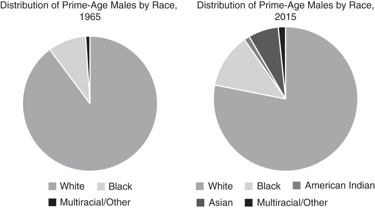
Figure 5.5 Distribution of prime-age males by race, 1965 vs. 2015

Figure 5.6 Work rates for prime-age males by race, 1965 vs. 2015

Figure 5.7 Distribution of prime-age males by race and ethnicity, 1971 vs. 2015

Figure 5.8 Work rate for prime-age males by race vs. ethnicity, 1971 vs. 2015
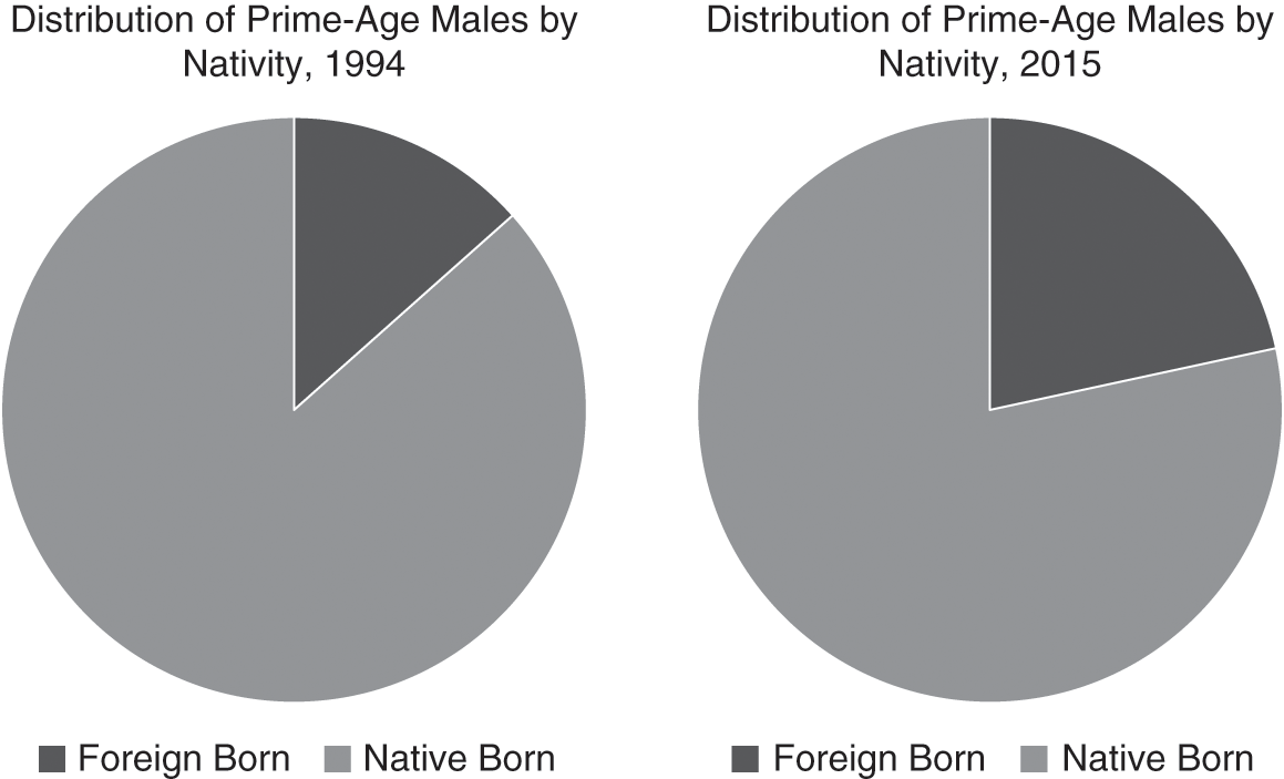
Figure 5.9 Distribution of prime-age males by nativity, 1994 vs. 2015

Figure 5.10 Work rates for prime-age males by nativity, 1994 vs. 2015
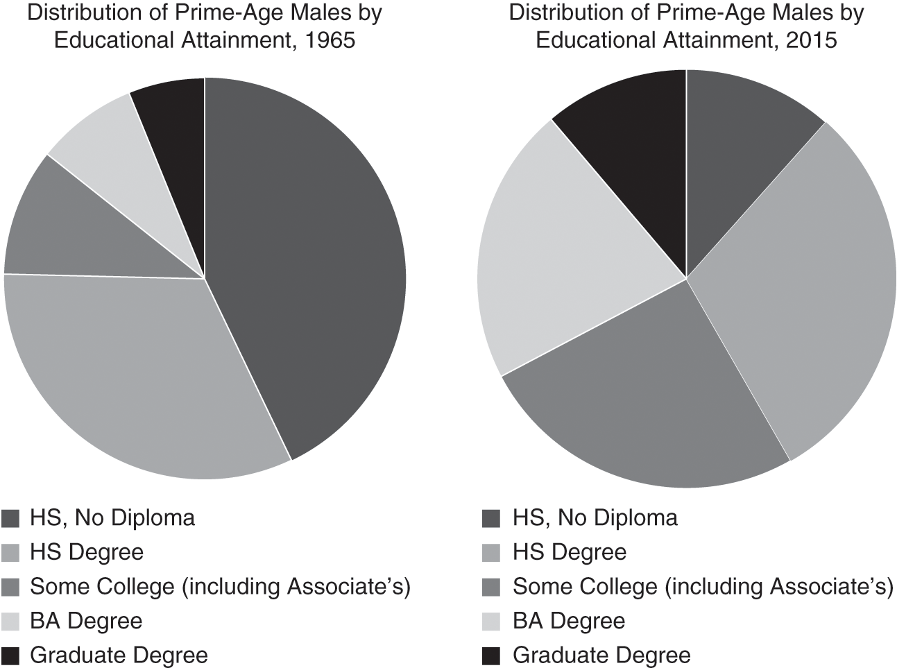
Figure 5.11 Distribution of prime-age males by educational attainment, 1965 vs. 2015

Figure 5.12 Work rates for prime-age males by educational attainment, 1965 vs. 2015

Figure 5.13 Distribution of prime-age males by marital status, 1965 vs. 2015
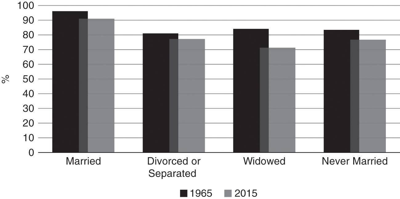
Figure 5.14 Work rates for prime-age males by marital status, 1965 vs. 2015
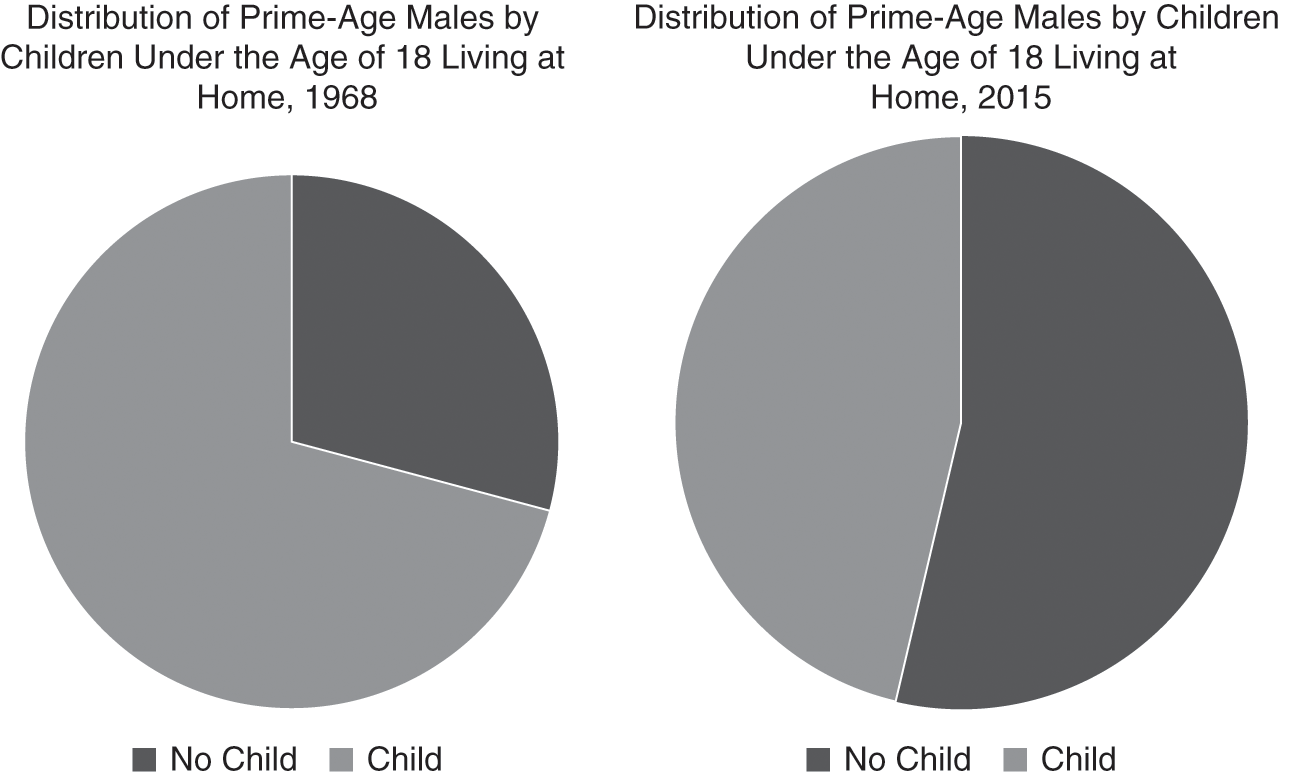
Figure 5.15 Distribution of prime-age males with children under the age of 18 living at home, 1968 vs. 2015

Figure 5.16 Distribution of prime-age males by family status and presence of child (<18), 1968 vs. 2015

Figure 5.17 Work rates for prime-age males by family structure, 1968 vs. 2015
Race and Ethnicity
The 1965 CPS offers just three alternatives for categorizing the “race” of the US population: White/Black/Multiracial. By 2015, the categories of Asian and Native American have also been added to the taxonomy. Between 1965 and 2015 the proportion of prime-age men identified as White dropped by about 12 percentage points, from roughly 90% to 78%. But roughly eight points of this twelve-point decline was due to the newfound availability of Asian and Native American classifications for 2015; almost all of whose contingents would have been represented as White under the 1965 schema. The only two consistent racial categories for the 1965–2015 period are Black and Multiracial/Other; the proportion of prime-age men identifying as Black rose by a little over 3 points, from around 9% to around 12%, while the proportion for Multiracial/Other rose by somewhat less than one point, from 1% to a bit less than 2%. In all, then, these “race” data do not seem to reveal any major shifts in US “racial composition” over the period in question (apart from the introduction of new categories) – in part perhaps because of the limitations of this classification system for modern America.
A more nuanced and informative picture of heritage and ancestry comes from the CPS information on “ethnicity,” which in addition to counting Asian and Other/Multiracial persons, also identifies the population of Hispanic origin (both White and Black), non-Hispanic Whites, and non-Hispanic Blacks. This CPS series commenced in 1971, and the breakdown from that year for prime-age men can be compared with results for 2015.
Between 1971 and 2015 the ethnic composition of US prime-age males changed appreciably. The most dramatic change was for the proportion of Hispanic men, which soared from under 5% to almost 18%. (Almost all of these Hispanic men classified themselves as White; as of 2015, less than 1% of all prime-age men were Black Hispanics.) In 2015, self-identified Asians comprised almost 7% of prime-age US men, and though I lack corresponding data for 1968, I may suspect the percentage was much smaller back then. Non-Hispanic Black men accounted for just under 12% of prime-age males in 2015, up about 2 percentage points from 1971. By 2015, non-Hispanic Whites (or “Anglos”) made up just 62% of the prime-age male population, down roughly 17–23 percentage points, depending on the initial number of Asians in the prime-age male pool in 1968. This is a considerable reduction in the “Anglo” proportion of the prime-age male population in somewhat less than half a century, but with only a very small part of the increase in the “minority” percentage (somewhere between less than an eighth and less than a tenth) due to an increase in the proportion of non-Hispanic Blacks.
For prime-age men overall, work rates fell by nearly 9 percentage points between 1965 and 2015, and by almost 8 percentage points between 1971 and 2015. Over those same years, Black and Non-Hispanic Black work rates fell even more sharply than this: By nearly 15 points and over 13 points, respectively. By 2015, roughly 27% of all prime-age Black or non-Hispanic Black men in the civilian noninstitutionalized population – over one in four – reported no paid work at all. The Black/White and non-Hispanic Black/non-Hispanic White gap in work rates widened over these decades: From 7 points in 1965/71 to 13-plus points in 2015. White/“Anglo” work rates fell somewhat less than the national average over these years.
The work rates for non-Hispanic Blacks in the prime-age male population in 2015 are thus perhaps akin to those for the United States during the darkest hours of the Great Depression – and there are other minority groups with similar grim prospects. In 2015, the prime-age male work rate for Native Americans was just 72% – meaning 28% had no paid work. Likewise, prime-age men with Multiracial backgrounds, as well as the small contingent who self-identified as Black Hispanic, were in groupings where over 20% had no paid work.
However, the story of the collapse of work for the modern American man is by no means an unrelieved story of differentially poor performance for ethnic minorities. By 2015, White Hispanics and Asians accounted for nearly one quarter of the prime-age male population – twice the number for non-Hispanic Blacks. Of all ethnic groups whose trends can be traced over the decades under consideration, the group with the best (or perhaps I should say least-bad) work rate trends are the Hispanics, whose work rates dropped by “only” 1 percentage point between 1971 and 2015.
By 2015, interestingly enough, both Hispanic and Asian work rates for prime-age men were slightly higher than those of “Anglos.” Not only has America become more ethnically diverse over the past half-century but diversity in work rates for America’s ethnic minorities has become more apparent as well. At the same time, these racial and ethnic differentials help place the dimensions of the postwar collapse of work for prime-age men in sharper perspective: Work rates for Blacks in 1965 were higher than for Whites fifty years later, and rates for non-Hispanic Whites in 2015 were just about the same as they had been for non-Hispanic Blacks back in 1971.
Nativity
Most of America’s changing ethnic complexion since 1965 is due to immigrants and their descendants, and much of this change is accounted for by the foreign-born themselves. CPS did not begin to track employment patterns by nativity until the 1990s, but even in just over two decades for which such data are available, we can see the impact on both prime-age male population composition and on overall prime-age male work rates.
In 1995, foreign-born men accounted for a little over 13% of all prime working-age males in the US civilian noninstitutionalized population. Just twenty-one years later, the corresponding proportion was nearly 22%. In 2015, foreign-born prime-age men were overrepresented in the employed population, meaning their work rates were higher than those of native-born men. (This turns out to be true, incidentally, for all major ethnic groups in America: Whites, Blacks, Hispanics, and Asians alike.)
Between 1994 and 2015, prime-age male work rates fell by a little over 3 percentage points, but trends for native- and foreign-born men moved in opposite directions: Down sharply for the former, up distinctly for the latter. Indeed, foreign-born men are the only group covered in my study for whom long-term work rates were reported to rise. As of 2015, work rates were over five points higher among prime-age men for the foreign-born than the native-born, and over four points higher than the national average.
Educational Attainment
In terms of sheer years of schooling, America was a much more educated society in 2015 than in 1965 – and of course the same was true for America’s prime-age men. In 1965, high school dropouts formed the largest single grouping within the prime-age male population, making up nearly 43% of the total; by 2015, they accounted for less than 12% of that population. Conversely, only 14% held a college degree or higher in 1965, as against nearly 33% in 2015. By 2015, nearly three fifths of America’s prime-age men had at least some college training in their résumé, as against just a quarter back in 1965.
From 1965 to 2015, work rates for prime-age men have always tracked positively with education: The higher the level of educational attainment, the higher the work rate. Over these decades, though, the gradient has grown far steeper. Work rates have declined for every educational attainment, but they have more or less collapsed for those at the lower end of the spectrum. Work rates for men with a graduate education fell by only 2 percentage points over that half-century, yet even for men with no bachelor’s degree but some college training, work rates dropped by eleven points. For men with just a high school diploma, rates plunged by nearly seventeen points, and for those with no high school diploma, they plummeted by almost eighteen points. By 2015, nearly 20% of prime-age men with high school diplomas but no higher training were jobless; the same was true for over 27% of high school dropouts, and the vast majority of these same jobless, lower educated men were entirely out of the labor market, no longer actively seeking employment. In retrospect, no less astonishing than the collapse in work for lower skilled men may be the high work rates those same educational groups still maintained just two generations ago. In 1965, after all, work rates for prime-age men with just a high school diploma were higher than those for men with graduate education today (i.e., 2015), and rates for high school dropouts in 1965 were over five points higher than the overall average for a the much more schooled prime-age male population of 2015.
Family Structure
Between 1965 and 2015, as in most other affluent Western societies, US marital patterns and living arrangements underwent upheaval, the reverberations from which are evident in my data on prime-age men. In 1965, five out of six prime-age men were currently married; by 2015, married men formed only a bare majority of that population. In 1965, less than a tenth of men aged 25–54 had never been married; by 2015, this group formed nearly a third of the entire prime-age male population. The proportion divorced or separated likewise roughly tripled over these decades. (The widowed proportion actually shrank slightly, but this was a tiny segment of the US prime-age male population: Less than 1% in 1965.)
This postwar disruption in previously extant family patterns is all the more evident from 1968 onward, once CPS began reporting on living arrangements and children. In 1968, nearly 70% of prime-age men were not only married, but married and living with at least one child under 18 years of age at home. By 2015, barely 40% of prime-age American men were married with children at home, while close to 30% were never married and currently not living with children. In all, less than half of all prime-age men – just 46% – were living with children in 2015; in 1968, by contrast, more than twice as many prime-age men had a child in their home as did not (70% vs. 30%).
This upending of previous living arrangement profiles, I should emphasize, was partly the result of declining fertility levels, which were considerably lower in 2015 than 1968 – but only partly. A major driver was the increasing likelihood that a man would not live in the same home as his children, irrespective of his marital status. By 2014, according to the Census Bureau’s Survey of Income and Program Participation (SIPP) survey, only three quarters of US men were living with all their identified biological children (Monte Reference Monte2017). This estimate, furthermore, only covers children those fathers reported or acknowledged. An analysis of SIPP data for the year 2004 noted that the average number of biological children reported by adult men was 20% lower than the number reported by adult women – a discrepancy possibly explained, in the words of the authors, by “underreporting in the survey or men not knowing about their offspring” (Emens and Dye Reference Emens and Dye2007).
Just as we observe major differentials in prime-age male work rates – both at any given point in time and also across time – by race or ethnicity, nativity, and education, so we do with family structure. Very broadly speaking, work rates are always higher for married men than for others, and almost higher for men with children at home, irrespective of their marital status.
Let us begin by looking just at marital status. In 2015, the work rate for all married men aged 25–54 was 91% – over 6 points higher than the national average. Work rates for these married men were roughly 14 points higher than for their never-married and separated/divorced peers, and nearly 20 points higher than for their widowed counterparts (although this is a tiny population – less than two thirds of a percent of the total). Interestingly enough, back in 1965, work rates for married men were already much higher than for others: 10 or more points higher than for those never married or widowed, and 13 points higher than for those separated or divorced. Work rates for married prime-age men did decline between 1965 and 2015, but by less than for any other marital status. Some may be surprised by how little work rates fell for never-married prime-age men over this half-century: The drop was a bit under seven points, as against an average drop of nearly nine points for prime-age men overall. Part of the answer to this apparent paradox may lie in the extraordinarily low levels to which work rates for never-married prime-age men had already dropped. In 1965, work rates for never-married prime-age men were already down to 83% – over 4 points below the national average that same year for Black prime-age men; fully 7 points below the level that same year for high school dropouts; and, despite an intervening half-century of sharp work rate declines, lower than the national average for prime-age men in 2015.
Now, let us consider the matter of prime-age men with children under 18 in their homes, biologically related or otherwise. In 2015, the work rate for any prime-age men with any children at home was 91% – almost the same as for the average for married prime-age men that same year. The gap in work rates separating prime-age male homes with and without children in them was almost 12 percentage points – a differential comparable to that separating college graduates and high school graduates in 2015, and almost as large as the 2015 White/Black work rate disparity for prime-age males. An appreciable gap in work rates between prime-age male homes with and without children was already apparent in 1968, but by 2015, that gap had close to doubled, meaning that work rates fell much further for childless homes than those with children in them.
I can further disaggregate work profiles by both marital status and presence of children for America’s prime-age men in 2015 and 1968.
In 2015, the prime-age work rate for married men with children at home was almost 93% – very slightly higher than for college graduates that same year. Married men without children at home reported work rates over six points lower; even so, their rates were above the overall average for 2015, and indeed, higher than for those of any other category of men not currently married. Whether or not they had children at home, prime-age men who were separated/divorced, widowed, or never married all reported work rates below the national average, but work rates tended to be lower still for those without children (excepting only never-married men, where the rates were very slightly higher for those without children at home).
In 1968, the relationship between work rates and family structure was similar (if not identical) to the patterns witnessed in 2015. Then as now, married men had the highest work rates, with the very highest reported by married men with children at home. (In 1968 the work rate for this “married with kids” contingent was over 96%!) The nonmarried men had lower work rates than their married counterparts, and for each of the other designations for marital status, men with children at home tended to have higher work rates than those who did not.Footnote 2 For those prime-age men not currently married and without children at home, work rates were already very low by 1968 – more or less on a par with America’s overall average prime-age male work rates for 2015, which, as we have already seen, were actually lower than prime-age male work rates in 1940, at the tail end of the Depression.
We can see from these comparisons that work rates had already commenced to collapse by the mid- or late 1960s among prime-age men with what we might call “nontraditional” family types (i.e., for those who were not currently married, and especially for those not currently married without children at home). The work rates for all not currently married men in 1965 were lower than the corresponding rates for either contemporary Black men or high school dropouts. Work rates for not currently married prime-age men without children at home – all “races” included – in 1968 were lower than for non-Hispanic Blacks of all family types in 1971. By such indications, the collapse of work rates for nontraditional family types preceded the great drop in work rates that were to come for both non-Hispanic Black and less highly educated prime working-age men in subsequent decades.
Examining the Relationship between Family Structure on Prime-Age Male Work Patterns
As we have seen, family structure – like race and ethnicity, nativity, and educational attainment – appears to be a powerful predictor of postwar work patterns for American men. We can begin to assess the impact of these social factors on changing male work profiles – on those major postwar declines in male work rates and dramatic upsurges in the percentages who have exited the workforce altogether – with two simple quantitative comparisons.
The first is to estimate the relative risk of being out of the workforce (or NILF, not in labor force) – a condition that mirrors the work ratio closely, albeit imperfectly – in accordance with given sociodemographic characteristics. The second is to present illustrative counterfactuals for the potential contribution of sociodemographic change on employment patterns. We derive this counterfactual by holding constant the characteristic-specific work rates or NILF rates for prime-age men for the year 2015, but applying these against the composition of the prime-age male population in 1965 (or whatever the earliest year for my analysis in the previous section may have been), so as to indicate what the NILF rates and work rates would have been like if the composition of the prime-age male population composition were the same nowadays as, say, half a century earlier.
Statistically speaking, these metrics cannot tell us how much changes in family structure have altered postwar male employment patterns. For one thing, changes in US family structure are correlated with other big social changes – in education, ethnicity, nativity, and other factors – which I do not attempt to disentangle in this section. For another, any statistical associations I uncover are just that – associations – in which questions of causation remain unanswered. Recognizing these important caveats, we can begin to quantify the relationship between family structure and the decline of work for the postwar American man.
Table 5.2 outlines the relative risk for prime-age men ending up in the NILF pool by social characteristic. The interpretation of the results is straightforward: Each cell indicates how much more likely, or less likely it is that the particular group of men in question will be represented in the NILF pool than the “average” prime-age US man in the year 2015.
Table 5.2 Who is more likely – and who is less likely – to be in the 7 million pool of prime-age NILF Males? Relative odds by demographic characteristic: 2015
| Race/Ethnicity | Educational Attainment | Marital Status | Nativity | ||||
|---|---|---|---|---|---|---|---|
| Hispanic | −20% | Graduate Studies | −59% | Married | −36% | Foreign-Born | −28% |
| Asian | −10% | Bachelor’s Degree | −43% | Divorced/Separated | +41% | Native-Born | +8% |
| “Anglo” (Non-Hispanic White) | −7% | Some College Training | −3% | Never Married | +48% | ||
| Multiracial | +31% | High School Diploma only | +25% | Widowed | +116% | ||
| Non-Hispanic Black | +71% | No High School Diploma | +77% |
Consider first the factor of race and ethnicity. In 2015, non-Hispanic Whites were about 7% less likely to fall into the pool of prime-age men neither working nor looking for work than would have been suggested by their overall numbers alone. This necessarily means that non-“Anglo” minorities as a whole were overrepresented in the prime-age male NILF population. Yet, there were strikingly divergent dispositions and risks here for different ethnic minorities. On the one hand, non-Hispanic Blacks were far more likely to be NILF than their national numbers alone would have suggested: They were overrepresented by 71%. By the same token, Multiracial men were 31% more likely to be NILF than would have been expected just from their population total. On the other hand, Asian men were less likely than “Anglos” to be NILF – 10% less likely than prime-age American men as a whole – while Hispanic men were 20% less likely to be NILF than American prime-age men overall. America’s prime-age men of color, in other words, included both the ethnicities most likely to have dropped out of the labor force, and those very least likely to have done so.
Now consider the variable of nativity. On the whole, native-born men are more likely to have dropped out of the workforce than would have been predicted by their proportion in the national prime-age population: They are overrepresented by about 8% in the NILF pool. On the other hand, foreign-born men are markedly underrepresented: 28% less likely than their proportion in the overall prime-age male population would have suggested. (We may note that the great majority of foreign-born men nowadays are Asian or Hispanic – groupings, as we have already seen, distinctly less likely to be NILF; thus ethnicity and nativity appear to be significantly overlapping factors.)
With respect to educational attainment, we see a stark and already quite familiar gradient of risk. At one extreme, prime-age men with a graduate education are nearly three fifths (59%) less likely to be found in the NILF pool than the overall average; at the other extreme, prime-age men without a high school diploma are over three quarters (77%) more likely to be NILF. In between these end points, men whose highest attainment was a college degree college were 43% less likely to be NILF than the population-wide average, while men with a high school diploma were 25% more likely to be NILF, and those with some college training were close to the nationwide average (3% below it). The powerful and predictable regularity of the correlation between educational attainment and employment in America is one of the widely accepted relationships in the contemporary social sciences, and Table 5.2 demonstrates the importance of this social factor with respect to prime-age NILF men.
Thus far, the strongest NILF risks identified in the US prime-age male population in 2015 are for non-Hispanic Blacks and for high school dropouts of all ethnicities: Note furthermore that the relative risk of being NILF is of roughly the same magnitude these two groups. We might assume that part of the explanation for this outcome would be the strong overrepresentation of African–American prime-age men in the pool of high school dropouts, but such an assumption would appear to be erroneous. Within the civilian noninstitutionalized population of prime-age men, the proportion of non-Hispanic Black men with no high school diploma is only very slightly higher than the national average for all races together: 10.2% vs. 9.7% in 2015.Footnote 3 Other powerful influences, apart from differences in educational attainment levels, must also be at work determining this highly unfavorable employment outcome for Black men in modern America.
Although perhaps less generally recognized than race/ethnicity and education, marital status and family structure turn out to be powerful predictors of male employment status, too. In 2015, widowed men were over twice as likely to be in the NILF pool as their totals in the overall population would have suggested, but as already mentioned, this was a very small contingent in terms of absolute numbers. On the other hand, the very large numbers of never-married men in 2015 were 48% more likely to be NILF than their population weighting would have suggested. Separated or divorced men were over 40% more likely to be NILF than the “average” prime-age man. By contrast, married men are 36% less likely to be neither working nor looking for work.
Much the same is true for the relationship between employment status and presence of children at home. In 2015, prime-age men with no children at home were 37% more likely than average to be NILF, while those with one or more children at home were 43% less likely. Even larger differentials are evident when I parse by both marital status and presence of children at home. On the one hand, currently married men with children at home are only half as likely to be NILF (–51%) as would be expected by their overall numbers; on the other, never-married men without children at home were nearly 50% (49%) more likely to be long-term absentees from the labor force than we would have expected from their total numbers.
Those numbers underscore just how powerful a predictor of employment status for prime-age men the factor of family structure appears to be. Consider the following: In Table 5.2, the odds of being a prime-age NILF male are 50% higher for the native-born than foreign-born; 84% higher for non-Hispanic Blacks than non-Hispanic Whites; and 119% higher for men with only a high school education in relation to those whose highest degree is a college degree. By comparison, the odds of being NILF were 127% higher for a prime-age man with no children at home than one living in a home with children: A gap far larger than the Black/White differential, and indeed, slightly greater than the high school/college differential. Similarly, the odds of being NILF were over 130% higher for never-married prime-age men than for those currently married. Even greater disparities in NILF risk were evident for prime-age men who were currently married with children at home as against never-married men with no children at home: Here the odds were over 200% higher for the latter, very nearly the same differential as for high school dropouts in relation to college graduates.
Suffice it then to say that differences in marriage patterns and family structures are strongly associated with employment differentials for prime-age men in contemporary America. A quick glance at Table 5.2 offers the impression that the influence of differences in family structure may roughly in the order of differences in educational attainment for prime-age male employment, or more specifically, the risk of being absent from the labor force. That impression is reinforced by estimates of conditional compositional effects in today’s (2015) prime-age male NILF rates and work rates: Holding 2015 work and NILF rates for subgroups constant, but recalculating hypothetical national rates on the basis of these subgroups’ weighting in society as they were back in 1965, or some other earlier benchmark year in the previous section of this chapter (see Figure 5.18).
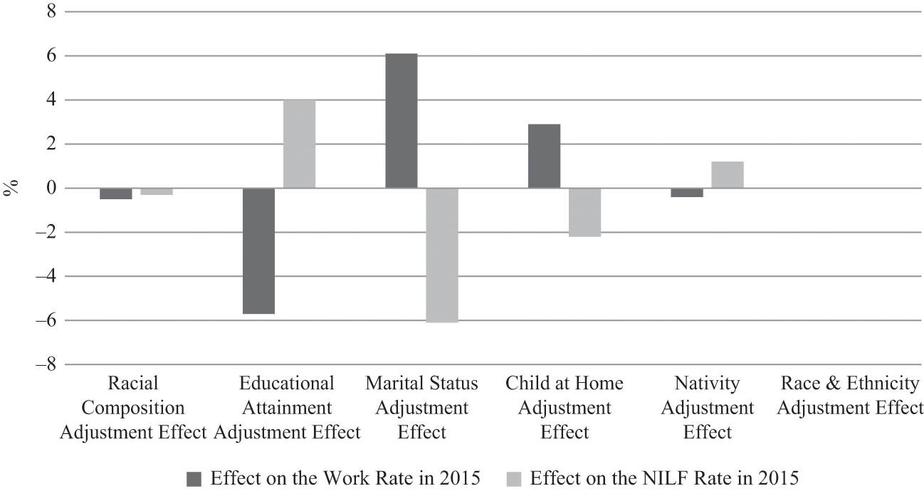
Figure 5.18 Conditional compositional effects on prime-age male work rates and NILF rates in 2015
Perhaps surprisingly, America’s shifting postwar racial and ethnic composition appears, by my calculations, to have had very little impact at all on changes in either work rates or NILF rates for prime-age men. Superimposing the 1965 “race” distribution for prime-age men on 2015 race-specific work rates results essentially in zero adjustment against either actual reported 2015 prime-age male work rates or their NILF rates. A very slight (half of 1 percentage point) downward adjustment in work rates would result from matching the 1971 racial and ethnic composition of the prime-age male population against work rates by ethnicity for 2015, while at the same time such an exercise would result in a downward reduction of NILF rates by less than one third of 1 percentage point. In effect, increasing ethnic diversity looks to have had little impact with respect to prime-age male employment status: Poor performance by non-Hispanic Blacks and some other less populous groupings were balanced out by the above-average performance of other groups, specifically Asians and Hispanics.Footnote 4
The conditional compositional effect for nativity looks to be somewhat larger than for race and ethnicity. With current (2015) nativity-specific work rates but a 1994 breakdown of population by nativity, prime-age male work rates would have been 0.4 percentage points lower in 2015 than those actually recorded – actual work rates over that period declined by 2.3 points. By the same token, the conditional compositional adjustment raises NILF rates by over one point; in actuality, NILF rates fell by about three points over that same period. These hypotheticals suggest that the overall employment profile of contemporary prime-age men would look worse, not better, without the intervening influx of foreign-born prime-age men.
Educational attainment, however, appears to exert a larger influence on adjustments for work rates and NILF rates than either race and ethnicity, or nativity. With 2015 education-specific work rates but 1965 distributions of educational attainment, the conditional calculation for prime-age male work rates would be 5.7 percentage points lower than those actually recorded in 2015, and the conditional calculation for NILF rates would be 4 points higher. Those hypothetical adjustments can be compared with the actual drop in work rates of 9.3 points, and the jump in NILF rates of 8.8 points. By these illustrative computations, improvements in educational attainment appear to have played a very important role in preventing a far worse decline in male work over the past half-century. Hypothetically speaking, with today’s education-specific rates and a 1965 distribution of educational attainment, the drop in prime-age male work rates would be over half again as dramatic as that which took place, and the jump in NILF rates would likewise be almost half again as large as what was actually recorded.
Big as these hypothetical conditional adjustment effects for educational attainment may appear, those for marital status are of the same magnitude – in fact, even a bit larger. Whereas the calculated compositional effect for changes in educational attainment for 1965–2015 on prime-age male work rates amounted to –5.7 points, it would be +6.1 points for marital status. Where the calculated compositional effect for educational attainment over those same years on NILF rates would be +4 points, it would be –5.7 points for marital status. By one reading, this might suggest that that the impact on prime-age male work rates and NILF rates from changes in marriage patterns would have been sufficient to cancel out the impact of half a century of improvements in educational attainment, entirely – and then some.
I may note as well that the conditional compositional effect for presence of children at home (using a 1968 benchmark) would adjust work rates upward by nearly 3 points (2.9 points) against their actual 2015 levels, and would adjust NILF rates downward by more than 2 points (–2.2 points). Even without more refined calculations, taking into account the marital status of men in homes with children, it is apparent that the “child at home factor” looks to be somewhat over half as large in magnitude as the educational attainment factor.
In this section, we have seen that marital status and family structure correlate strongly with employment status for prime-age men nowadays – indeed, that the predictive power of family structure on work rates and NILF rates are on a par with that of education, which is commonly recognized as an extremely powerful factor in social outcomes. We have also seen that changes in family structure over time could be associated with changes in male work patterns over time, and that, here again, the conditional compositional effect on male employment patterns over the past half-century might be of the same absolute magnitude as improvements in educational attainment, albeit weighing in the opposite. However, we need to look at these relationships more closely to draw inferences about the independent statistical contribution of changes in family structure to changes in male work patterns, to say nothing about causality or the possible casual mechanisms at play here.
Is Family Structure a Determinant of Postwar Male Work Patterns?
Establishing a correlation or association between two factors – even a strong one – is not the same thing as establishing an independent and causal influence of one factor on the other. For one thing, such associations may be due to additional, unobserved conditions or variables with which both observed factors happen to correlate. However, even if a genuinely independent and statistically meaningful relationship can be established between two factors, that correlation tells us nothing about the direction of causality: In statistical jargon, we cannot tell which variable is independent and which is dependent simply by demonstrating that a relationship exists in the first place.
In the context of the family structure/male employment relationship, these cautionary methodological generalizations have at least two immediate and practical implications. First, it could be possible that the correlation we have detected between family structure and male employment patterns are in reality due largely, or entirely, to a deeper underlying relationship between male employment patterns and some other factor closely tracking with changes in family structure: Educational attainment, for example, or race and ethnicity, or health. Second, even if a methodologically sound and independent relationship between family structure and male employment patterns could be identified, this would tell us nothing about which variable was influencing which. Far from assuming that family structure is affecting employment patterns, one might instead make the case that the declining availability of work for men is forcing a disintegration of traditional family patterns, as ever greater numbers of disadvantaged men find it impossible to find spouses and earn the wherewithal to form families. As it happens, recent social science studies include methodologically sound research by authors pointing the arrow of causality in each of these opposing directions (Ahituv and Lerman Reference Ahituv and Lerman2007; Autor, Dorn, and Hanson 2017).
An exhaustive examination of these methodological issues cannot be undertaken in this brief section; It will suffice instead to make two simple points. First, controlling for such important social factors as race/ethnicity and education does not eliminate the strong relationship between family structure and male employment patterns. Second, while the “declining male work causes declining male marriage” interpretation of causality is inherently plausible, and may indeed persuasively speak to part of the observed association between employment and family structure for US men, it also leaves a number of important aspects of the contemporary social tableau manifestly unexplained.
Consider, to begin, the potentially confounding factors of race/ethnicity and education. It is true that each of two factors tends to correlate with family structure and male work rates at one and the same time. With respect to ethnicity, Asian prime-age men report the highest proportion of those currently married and among the highest work rates; conversely, non-Hispanic Blacks report among the lowest numbers currently married and among the lowest work rates. By the same token, with respect to education, overall work rates and proportions currently married are lowest for prime-age men without a high school diploma and highest for those with a college degree or graduate education.
Clearly, race and education have a bearing on family structure in modern America, but when I attempt to control for them, a residual independent “family structure” effect is revealed, and its association with male employment profiles appears to be a strong one.
As already mentioned, a significant differential separates workforce participation rates for currently married and never-married prime-age men of every major US ethnic or “racial” grouping: White, Black, Hispanic, and Asian. As we already know, overall prime-age male NILF rates are much lower for Blacks than Whites 18.8% vs. 10.0% in 2015. Nevertheless, workforce participation rates for prime-age married Black men are distinctly higher nowadays than those for never-married White men, and have been for decades (see Figure 5.19). In this particularly vivid example, the “marriage effect” trumps the “race effect” – and it is by no means the only such example that could be adduced.
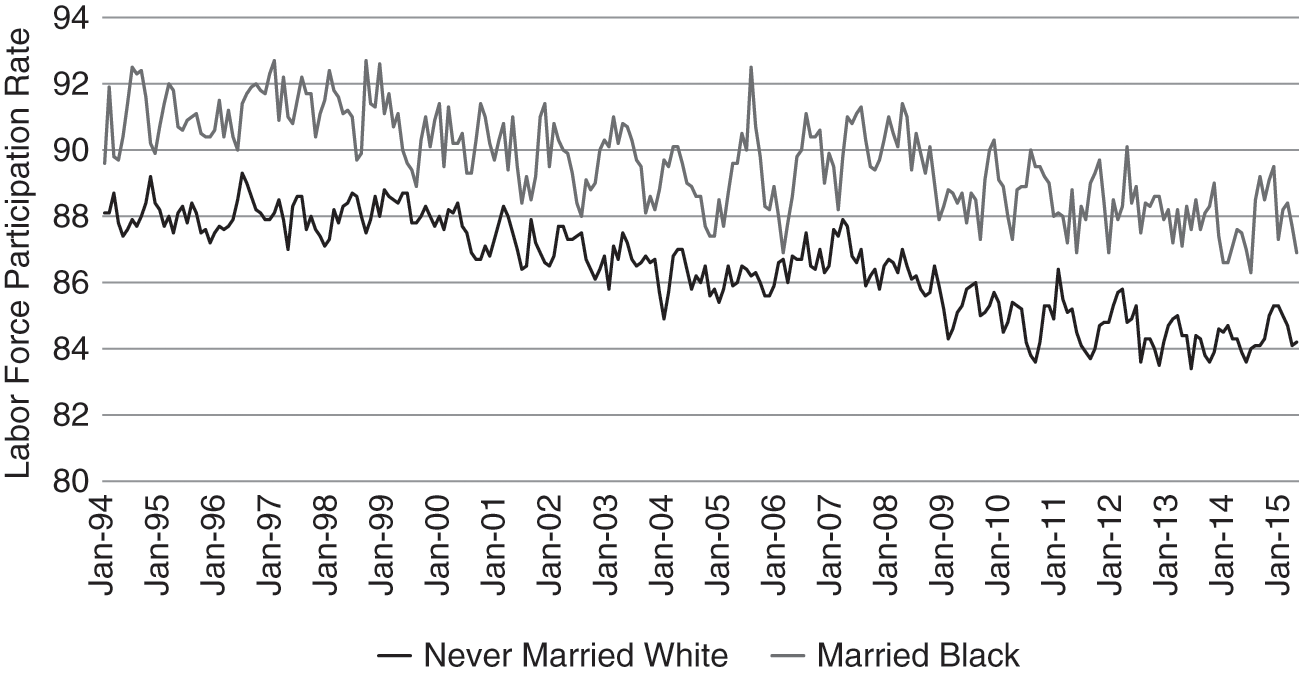
Figure 5.19 Labor force participation rate for males aged 25–54 by marital status and race: married Black vs. never-married White
To be sure, Figure 5.19 does not control for education, and it is possible that the educational profile of married Blacks could be different from (and more favorable than) that of their never-married White peers. However, if we look at education, we find that currently married prime-age men of all ethnicities report higher workforce participation if they are currently married than not currently married (divorced/separated, widowed, or never married) – and that this holds for every level of educational attainment. The lower the level of educational attainment, the greater the gap in workforce participation between men who are married and men who are not. Indeed, despite their ostensible disadvantages in the contemporary labor market, married high school dropouts record roughly the same workforce participation rates as never-married college graduates (see Figure 5.20). Here we see a particularly instructive instance of the “marriage effect,” one in which it apparently compensates entirely for the “education effect” with regard to workforce participation rates for prime-age American men.

Figure 5.20 Labor force participation rate for males aged 25–54 by marital status and educational attainment: never married with bachelor’s degree or higher vs. married high school dropout
I could provide similar examples of the effect of marital status after controlling for race and education, and analogous examples for the influence of the “child at home” effect after controlling for other social factors, but the point should already be clear: Even after controlling for other social factors, we see a strong residual “family structure” effect in play after taking such formidable social forces as race and education into account. The plain fact is, all other things being equal, currently married prime-age men appear to have consistently higher work rates and consistently lower NILF rates than those whose are not currently married – and the same holds true for prime-age men who have children living in their home.
Isolating a “marriage effect” or a “family structure effect,” of course, does nothing to clarify the direction of causality between changes in employment patterns and changes in family patterns. An inherently plausible case can be made that the decline of work is driving the decline of marriage and family formation for men. In this interpretation, the key factor in the decline of male work is a decline in the demand for male labor due to structural economic change: Technological change, globalization and trade, decline of manufacturing, outsourcing and all the rest. (The important 2016 study on the decline in prime age male labor force participation rates by the President’s Council of Economic Advisers is representative of this broadly accepted school of thought.) By this assessment, for example, demand for lower skilled male labor has fallen disproportionately over the postwar era, so marriage among lower skilled men has also fallen disproportionately during the postwar era.
On the face of it, this “demand-side” hypothesis would seem to have much to commend it. I would certainly not contest the proposition that it can explain some, perhaps even much, of the decline in employment for prime-age men over the past two generations. However, it clearly cannot explain all of it. In a number of important respects, the labor market patterns for prime-age men that have unfolded over the past half-century look to be fundamentally inconsistent with the “demand-side” hypothesis – and thus with the assessment that causality leads from changes in work patterns to changes in family structure.
Three empirical challenges to the “demand-side” theory deserve particular attention. The first is the trajectory of the prime-age male “inactivity rate” – the percentage of men not in the workforce – over the 1965–2015 period (see Figure 5.21). The trouble for the “demand-side” theory is the remarkable regularity of this trend: It is almost a straight line upward for fully fifty years. There is no indication whatever of any influence of the business cycle: The Great Recession of 2008/09 is not visible, nor for that matter are any of the previous six recessions that occurred over the decades between 1965 and 2008. Likewise with respect to trade shocks, it is impossible to detect the NAFTA agreement, or of China’s entry into the WTO, in the steadily increasing inactivity rates over these years. As with regard to technological disruptions, it is impossible to identify from the prime-age male inactivity rate the trend line for the advent of personal computers, Internet use, or any of the other great innovations that may have had a profound or disruptive effects on the demand for labor over these years. While the remarkable smoothness of the ascent in inactivity rates does not concord with any of these many major “demand-side” shocks, we note that it does track with the relative smoothness of the trends in changing family structure over the past two generations at the aggregate or national, level.

Figure 5.21 Rate of nonlabor force participation from 1965 to 2016: US civilian noninstitutionalized males aged 25–54
Second, there is the curious and, for the labor market-driven causality theory, rather inconvenient pattern of prime-age male inactivity rates at the state level (see Figure 5.22). From 1980 to 2014, interstate variations in such inactivity rates steadily increased, even though one would ordinarily expect a nationwide labor market to seek equilibrium in the wake of demand shocks. Furthermore, some of the states with the very highest prime-age male inactivity rates (for example, Maine) happened to border some of the states with the very lowest inactivity rates (e.g., New Hampshire – Maine’s only land boundary within the United States). On first impression, these growing state-level imbalances do not look like “demand-side” problems but rather “supply-side” problems: Insufficiency of migration or mobility. However, it should be remembered that the family structure-to-employment profile causation hypothesis is also a “supply-side” labor theory, since it implicitly posits that men who are not currently married and/or do not have children at home are less likely to seek work than those who do.
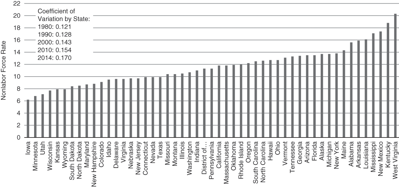
Figure 5.22 Nonlabor force rates among prime-age males by state (2015)
Finally, there is the matter of the wildly disparate workforce participation rates for less skilled men in accordance with their marital status (see Figure 5.23). According to CPS data, in 2015, a gap of almost 20 percentage points separated labor force participation rates for currently married and never-married prime-age male high school dropouts. This means that between 1965 and 2015 prime-age male LFPRs fell by about 8 percentage points for unmarried high school dropouts – somewhat less than for the prime-age male population as a whole – while they fell by almost 28 percentage points for never-married high school dropouts. If we attempt to explain this extraordinary disparity in outcomes as a “demand-side” effect, we are also obliged to come up with an explanation for why the demand for labor would drop so very little for less skilled men with more traditional family structures, and so radically for those with alternative family structures. To date, I am unaware of any such theorizing yet attempting such acrobatics.

Figure 5.23 Labor force participation rate for males aged 25–54 by marital status and educational attainment lower than a high school diploma
These few pages can only begin to address the complexities of a quantitative investigation of family structure as a determinant of male employment patterns in contemporary America. What I hope to have demonstrated, however, is that further rigorous examination of this topic is warranted, as there appears to be evidence of an independent relationship between family structure and employment patterns after holding other potentially confounding variables constant – and reason as well to believe there may be some genuine causal relationship between changes in family structure and changes in male employment patterns in postwar America (in additional to whatever causal relationships may work in the other direction).
Concluding Observations
This chapter has made the case that changing patterns for marriage and living arrangements correspond strongly with changing patterns of male employment in the United States over the postwar era, or, to offer a formulation perhaps more in keeping with the framing of this volume, that there is a strong relationship between increasing family inequality and increasing male employment inequality in contemporary America. I have offered evidence that differences in family structure track with differences in male employment patterns, even after taking account of alternative and perhaps competing social factors, such as race/ethnicity and education. Furthermore, I have offered evidence of a causal relationship between changes in family structure and changes in male employment patterns – evidence that the competing hypothesis of employment (“demand-side”)-driven changes in family patterns cannot explain readily, if at all. This chapter does not presume to undertake an exhaustive examination of the topic, but it does attempt to provide sufficient groundwork to justify and encourage further and more exhaustive research in this area.
It may be suitable to conclude by indicating some potentially fruitful directions for such work. This chapter established evidence of broad relationships on the basis of aggregate “macro”-statistics of a cross-sectional nature. For delving deeper into the dynamics of this relationship, and for teasing out possible causal mechanisms, quantitative analysis microdata would appear to be most suitable – and ideally, microdata from a longitudinal survey, as such information would help us better understand how and whether male employment behavior changes in the aftermath of changes in marital status or living arrangements.
It might also be beneficial, if possible, to add several additional social variables I did not include in my examination for this study. One of these would be prime-age male utilization of government benefits, including means-tested benefits and disability program benefits. Broadly speaking, we know that unemployed men are more likely to participate in such programs nowadays than employed men, and that NILF men are more likely to participate in them than unemployed men, but the interplay with family structure, and the issue of “demand-side” versus “supply-side” drivers of such increased participation, surely deserves more careful illumination. Another, and scarcely less important, variable would be criminal justice system history – in particular, previous criminal conviction record or comparable serious criminal history. Between the early 1960s and 2010, the number of adults in the United States with a criminal record is estimated to have more than quadrupled (Shannon et al. Reference Shannon, Uggen, Schnittker, Thompson, Wakefield and Massoglia2017). Rough calculations suggest that something like one in eight adult men not behind bars in the United States may have a criminal conviction in his past – the figure for prime-age men today may be even higher (Eberstadt Reference Eberstadt2016). Criminal justice status may possibly be the most important typically unexplored variable in social research on the dynamics of change in family structure and male employment. Casting light on this strangely unexplored dimension of modern American life would surely permit us to clarify and refine our understanding of the dynamics of family inequality and employment inequality in modern America.
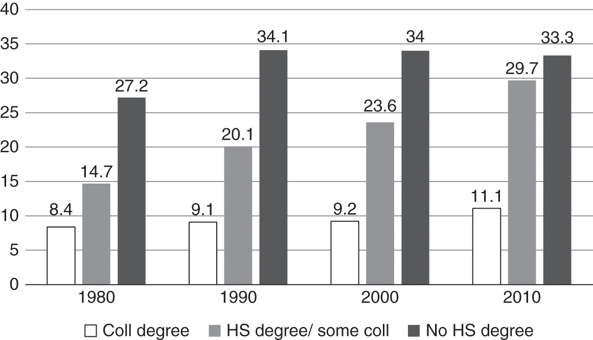
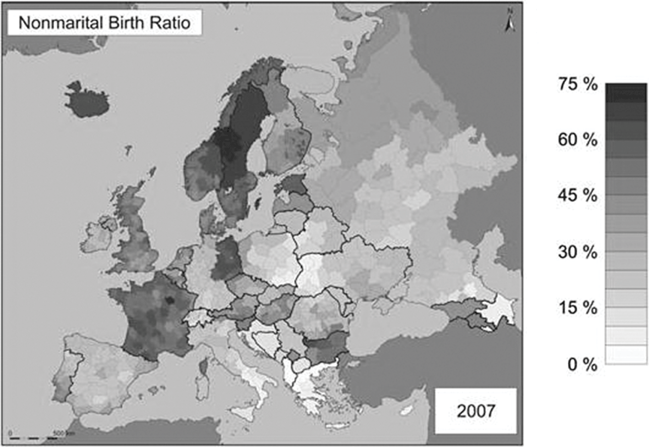

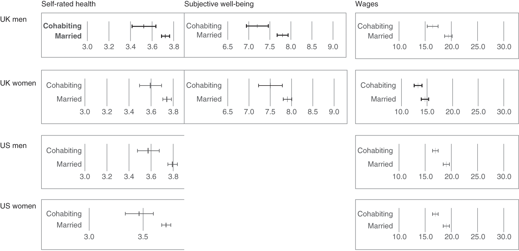


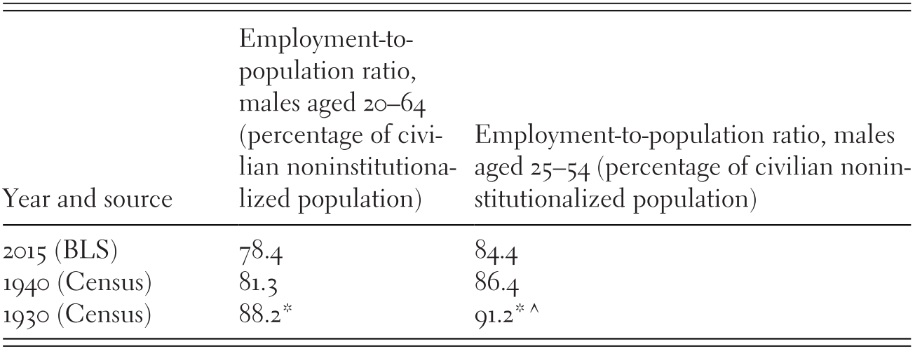

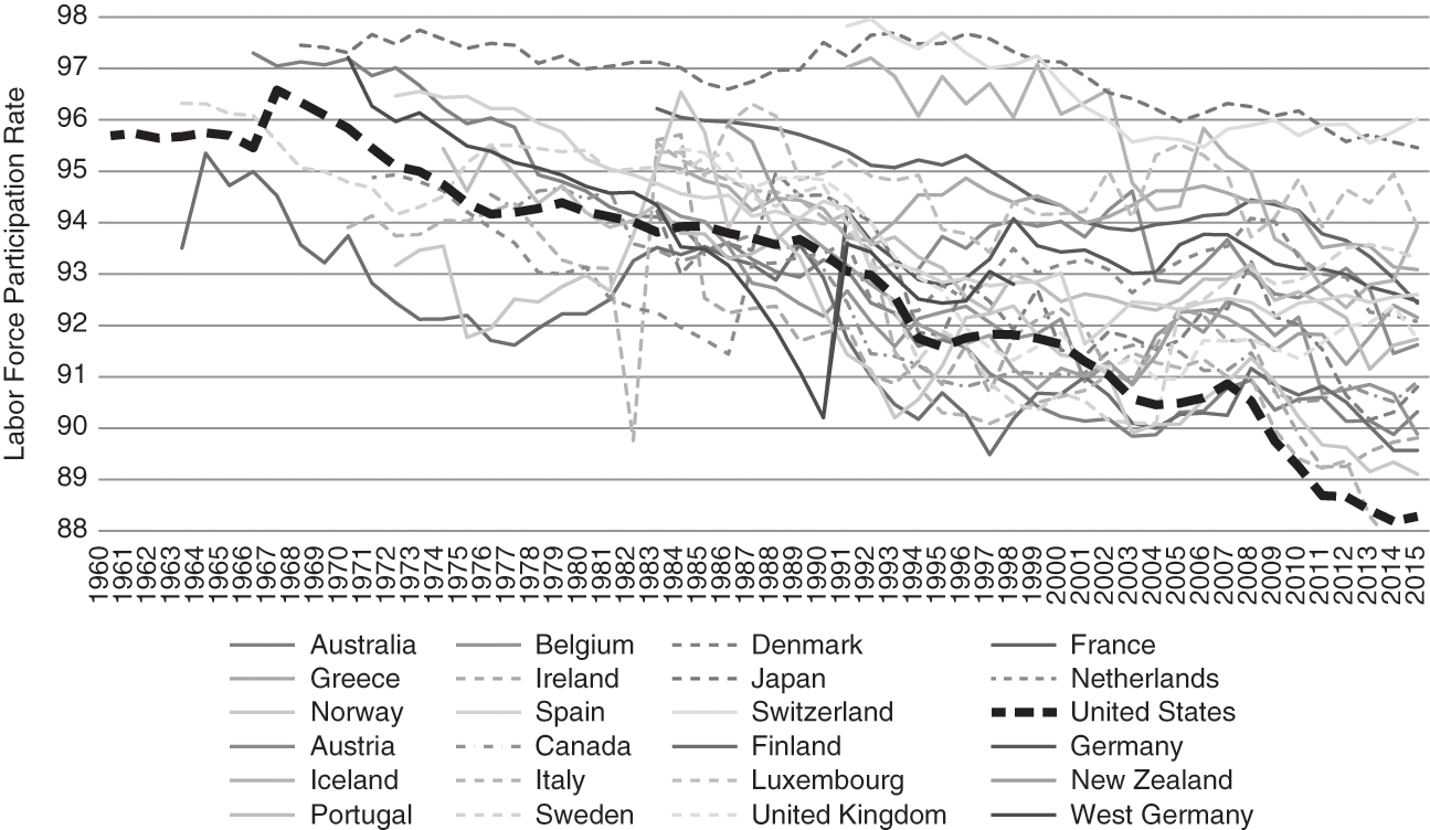


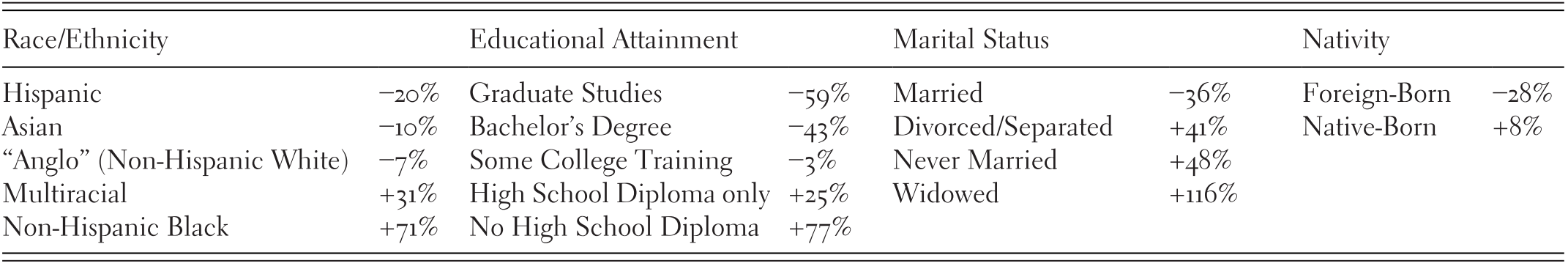


 Open access