


1. Introduction
Response flows driven by libration (small-amplitude harmonic modulation of the fast mean rotation) in axisymmetric containers (spheres, spherical shells, cylinders, annuli) are solely driven by viscous torques. On the other hand, in non-axisymmetric containers, the motions of the walls are not solely tangential to the walls and the effects of the resulting pressure torques can be dominant. These are present as topographic effects in practical situations, but the typically irregular topography leads to challenges in their systematic investigation. A cube rotating about an axis that is neither parallel nor orthogonal to any of its walls provides a simple geometry in which pressure torques are important and yet still allows for both efficient modelling and numerical simulations as well as precise experiments. Of particular interest is how the reflections of inertial wavebeams in rotating containers with some walls neither parallel nor orthogonal to the mean rotation axis introduce peculiar consequences (Phillips Reference Phillips1963), such as their focusing either into interior regions (Maas Reference Maas2001; Manders & Maas Reference Manders and Maas2003; Maas Reference Maas2005; Jouve & Ogilvie Reference Jouve and Ogilvie2014; Klein et al. Reference Klein, Seelig, Kurgansky, Ghasemi, Borcia, Will, Schaller, Egbers and Harlander2014; Sibgatullin & Ermanyuk Reference Sibgatullin and Ermanyuk2019; Boury et al. Reference Boury, Sibgatullin, Ermanyuk, Shmakova, Odier, Joubaud, Maas and Dauxois2021) or onto edges or vertices of the container (Greenspan Reference Greenspan1969; Beardsley Reference Beardsley1970; Troitskaya Reference Troitskaya2010a,Reference Troitskayab; Wu, Welfert & Lopez Reference Wu, Welfert and Lopez2020).
In this paper, we investigate numerically the flow in a cube rapidly rotating about an axis passing through the midpoints of two opposite edges, subjected to small-amplitude librational forcing. In this orientation, two opposite walls of the cube are parallel to the mean rotation axis while the other four walls are oriented obliquely at  ${\pm }{45}^{\circ }$ with respect to the mean rotation axis. The study of this orientation completes the investigation of the impacts of libration on the trilogy of proper rotations of the cube (see figure 1 for schematics of the three scenarios). The first case of the trilogy, where a cube rotating around an axis passing through the centre of two opposite faces, with all faces of the cube either parallel or orthogonal to the axis of rotation, was studied by Maas (Reference Manders and Maas2003) in the linear inviscid setting. Boisson et al. (Reference Boisson, Lamriben, Maas, Cortet and Moisy2012) studied this case experimentally by subjecting the cube to small amplitude librational forcing, and Wu et al. (Reference Wu, Welfert and Lopez2018) reproduced their experimental observations using direct numerical simulations of the Navier–Stokes equations. With none of the cube walls aligned obliquely to the mean rotation axis, the response flows consisted of resonantly excited inertial eigenmodes of the unforced rotating cube together with internal shear layers whose orientations are governed by the linear inviscid dispersion relation. For certain forcing frequencies in the inertial range (libration forcing frequencies less than twice the mean rotation of the cube), the inertial beams retraced and the modes resonated. The second case of the trilogy was studied in Wu et al. (Reference Wu, Welfert and Lopez2020), with the cube mean rotation axis being a diagonal passing through two opposite vertices, such that all walls of the cube are oblique to the rotation axis. In this case the response flows are dominated by inertial wavebeams emitted from some edges and/or vertices of the cube, depending on the libration frequency. Due to the peculiar reflection laws for inertial wavebeams at oblique walls, intricate patterns of intersecting and focusing wavebeams emerged for low Ekman numbers (ratio of mean rotation period to viscous time), which were remarkably well reproduced using a vector-based approach for the inviscid reflection laws.

Figure 1. Schematics of the cube librating about a rotation axis,  $\hat {\boldsymbol {\xi }}$, passing through (a) the centre of opposite faces, considered in Boisson et al. (Reference Boisson, Lamriben, Maas, Cortet and Moisy2012) and Wu, Welfert & Lopez (Reference Wu, Welfert and Lopez2018), (b) opposite vertices, considered in Wu et al. (Reference Wu, Welfert and Lopez2020) and (c) the centre of opposite edges (present study).
In the two earlier studies, both the Ekman number,  $E$, and the relative forcing amplitude,
  $\epsilon$, were kept equal and small, down to
  $E=\epsilon =10^{-6}$ in Wu et al. (Reference Wu, Welfert and Lopez2018) and
  $E=\epsilon =10^{-7}$ in Wu et al. (Reference Wu, Welfert and Lopez2020). With small
  $E$, the fast rotation provides a strong restorative force and any small disturbances introduced into the interior of the container are constrained to being circularly polarized inertial waves aligned with the characteristics (Greenspan Reference Greenspan1968). Keeping the libration amplitude,
  $\epsilon$, small results in the response flow being a synchronous periodic flow, invariant to the spatio-temporal symmetries of the forced system, whose velocity magnitude (relative to the mean solid-body rotation) scales linearly with
  $\epsilon$. For the present study, we are able to further reduce the Ekman number and the relative forcing amplitude by one order of magnitude to
  $E=\epsilon =10^{-8}$ by implementing a new numerical scheme with improved numerical stability characteristics and a third-order accurate temporal integration scheme. The governing equations and their symmetries, and the numerical technique used to solve them are described in § 2. Section 3 presents details of the forced response flow over the whole range of forcing frequencies supporting wavebeams. It is shown to consist, as in Wu et al. (Reference Wu, Welfert and Lopez2020), of unsteady boundary layers on the faces of the cube which meet at edges, with vortex sheets entering into the interior from select edges depending on the forcing frequency. We use the linear inviscid theory developed in Wu et al. (Reference Wu, Welfert and Lopez2020) to trace wavebeams from the edges from which they emerge all the way to the edges and vertices where they focus, following multiple reflections off faces and, possibly, edges. The theoretical predictions are compared in § 5 with the viscous nonlinear simulations from § 3. At low forcing frequencies, the focusing renders nonlinear and viscous effects non-negligible, even in the
  $E=\epsilon =10^{-8}$ case. As noted by Busse (Reference Busse2010), experimental measurements of responses to low-frequency librational forcings are missing from the literature. Simulations and theory in the vanishing forcing frequency regime are also scarce.
2. Governing equations and numerics
Consider a cube of side lengths  $L$, completely filled with an incompressible fluid of kinematic viscosity
  $\nu$ and rotating at a mean rate
  $\varOmega$ that is modulated harmonically at a frequency
  $\sigma$ with amplitude
  $\Delta \varOmega$. The system is non-dimensionalized using
  $L$ as the length scale and
  $1/\varOmega$ as the time scale, and described in terms of a non-dimensional Cartesian coordinate system
  $\boldsymbol {x}=(x,y,z)\in [-0.5,0.5]^{3}$ that is fixed in the cube, with the origin at the cube centre, and the corresponding non-dimensional velocity field is
  $\boldsymbol {u}=(u,v,w)$. The direction of the rotation axis is
  $\hat {\boldsymbol {\xi }}=(0,1,1)/\sqrt {2}$, and the non-dimensional angular velocity is
 \begin{equation} \boldsymbol{\varOmega}(t)=[1+\epsilon \cos(2\omega t)]\,\hat{\boldsymbol{\xi}}, \end{equation}
where the non-dimensional libration frequency  $2\omega =\sigma /\varOmega >0$, and the relative amplitude
  $\epsilon =\Delta \varOmega /\varOmega$ is the corresponding Rossby number. Figure 2 shows a schematic of the system. The non-inertial frame of reference attached to the librating cube introduces both Coriolis and Euler body forces into the (non-dimensional) governing equations
 \begin{equation} \frac{\partial \boldsymbol{u}}{\partial t} +(\boldsymbol{u}\boldsymbol{\cdot}\boldsymbol{\nabla})\boldsymbol{u} +2\boldsymbol{\varOmega} \times \boldsymbol{u} + \frac{{\rm d}\boldsymbol{\varOmega}}{{\rm d}t} \times \boldsymbol{x}={-}\boldsymbol{\nabla}p +E\nabla^{2}\boldsymbol{u}, \quad \boldsymbol{\nabla}\boldsymbol{\cdot}\boldsymbol{u}=0, \end{equation}
where  $E=\nu /\varOmega L^{2}$ is the Ekman number and
  $p$ is the reduced pressure which incorporates the centrifugal force. In this frame of reference, the no-slip boundary conditions are
  $\boldsymbol {u}=\boldsymbol {0}$ on all six walls of the cube. The two faces of the cube at
  $x=\pm 0.5$ are parallel to the axis of rotation. The four remaining faces are inclined at
  $\pm {45}^{\circ }$ relative to the rotation axis
  $\hat {\boldsymbol {\xi }}$. Four of the edges are orthogonal to
  $\hat {\boldsymbol {\xi }}$, while the remaining eight edges are inclined at
  $\pm {45}^{\circ }$ relative to
  $\hat {\boldsymbol {\xi }}$.

Figure 2. Schematic of the cube librating about the rotation axis,  $\hat {\boldsymbol {\xi }}=(0,1,1)/\sqrt {2}$, and three planar cross-sections used for enstrophy density visualizations. The
  $y=z$ plane is a meridional plane with its ‘top’ and ‘bottom’ corresponding to the two polar edges of the cube and the sides are diagonals of the two walls of the cube parallel to the rotation axis. The plane
  $x=0$ is another meridional plane, the ‘top’ and ‘bottom’ corners are the poles where the rotation axis bisects the polar edges of the cube and the side corners bisect the two equatorial edges of the cube. The plane
  $y=-z$ is the equatorial plane, orthogonal to the rotation axis; its ‘top’ and ‘bottom’ are the two equatorial edges of the cube and its sides are the other diagonals of the two walls of the cube parallel to the rotation axis.
In order to study the flow response to librational forcing in the fast mean rotation and small forcing amplitude regimes, the Ekman number  $E$ and forcing amplitude
  $\epsilon$ should be as small as is practical. To put this into perspective, experiments on a librating cube typically have
  $E\sim 10^{-5}$ and
  $\epsilon \sim 10^{-2}$ (Boisson et al. Reference Boisson, Lamriben, Maas, Cortet and Moisy2012), and in the related numerical study, Wu et al. (Reference Wu, Welfert and Lopez2018) used
  $E=\epsilon =10^{-6}$. In the Coriolis platform at Grenoble, the radius is approximately 6.5 m and the maximum rotation rate is approximately
  $0.008\ {\rm rad}\ {\rm s}^{-1}$, so using water at room temperature results in a smallest achievable Ekman number of approximately
  $3\times 10^{-6}$ (Godeferd & Moisy Reference Godeferd and Moisy2015). For the present study, we have been able to reduce these to
  $E=\epsilon =10^{-8}$ by employing a more robust and numerically unconditionally stable spectral scheme developed by Wu, Huang & Shen (Reference Wu, Huang and Shen2022). At present, how small an
  $E$ can be considered is limited not by numerical issues but rather by the available memory to process the solutions, which require greater spatial resolution as
  $E$ is further reduced.
The governing system is discretized in space using the Legendre–Galerkin spectral approach of Shen (Reference Shen1994), with Legendre polynomials of degree  $m$ for the velocity components and
  $m-2$ for the pressure in all three directions, with
  $m$ ranging from
  $m=50$ for the largest Ekman numbers considered to
  $m=350$ for
  $E=10^{-8}$. The resulting semi-discrete system is integrated in time using a consistent splitting scheme for the Navier–Stokes equations, introduced in Guermond & Shen (Reference Guermond and Shen2003), together with the scalar auxiliary variable stabilization scheme for general dissipative systems, developed in Huang, Shen & Yang (Reference Huang, Shen and Yang2020). The resulting scheme is unconditionally stable, third-order accurate in time for both the velocity and the pressure and only requires the solution of decoupled linear systems with constant coefficients at each time step. For all values of the Ekman number
  $E$, the number of time steps per forcing period used ranges from
  $100$ at high forcing half-frequencies,
  $\omega \geqslant 0.1$, to as many as
  $6400$ for
  $0.01\leqslant \omega \leqslant 0.09$. The solution,
  $\boldsymbol {u}$ and
  $p$, at an instant in time for
  $E=10^{-8}$ has
  $4\times 3\times 351^{3}\approx 5\times 10^{8}$ degrees of freedom (the factor 4 accounting for the three components of velocity plus pressure, and the factor 3 accounting for the three stages needed for the third-order temporal scheme). This results in a file of size 4 Gb using double-precision floating point numbers.
The governing equations and boundary conditions are invariant to  $\mathcal {R}$, a discrete rotation of angle
  ${\rm \pi}$ about
  $\hat {\boldsymbol {\xi }}$, and to
  $\mathcal {S}$, a reflection through the ‘equatorial plane’
  $y=-z$ (this plane is shown in the last panel of figure 2). The actions of these two symmetries on the velocity are
 $$\begin{gather} {\mathcal{R}}:[u,v,w](x,y,z,t) \mapsto [{-}u,w,v]({-}x,z,y,t), \end{gather}$$
 $$\begin{gather}{\mathcal{S}}:[u,v,w](x,y,z,t) \mapsto [u,-w,-v](x,-z,-y,t). \end{gather}$$
Their composition,  $\mathcal {C}=\mathcal {R}\mathcal {S}=\mathcal {S}\mathcal {R}$, is a centrosymmetry whose action is
 \begin{equation} {\mathcal{C}}:[u,v,w](x,y,z,t) \mapsto [{-}u,-v,-w]({-}x,-y,-z,t). \end{equation}
As the system is periodically forced, with period  $\tau ={\rm \pi} /\omega$, it is invariant to the time translation symmetry
 \begin{equation} {\mathcal{T}}:[u,v,w](x,y,z,t) \mapsto [u,v,w](x,y,z,t+\tau). \end{equation}
 Keeping the librational forcing amplitude  $\epsilon$ small, the responses are symmetric limit cycle flows synchronous with the forcing, with the Euclidean magnitude of
  $\boldsymbol {u}$ linearly proportional to
  $\epsilon$, with
  $\boldsymbol {u}\to \boldsymbol {0}$ as
  $\epsilon \to 0$. This scaling has been tested using a range of
  $\epsilon$ for fixed
  $E$, with
  $\epsilon < E^{1/2}\ll 1$. All reported results were obtained using
  $\epsilon =E$. All of this makes it convenient and appropriate to introduce a scaled velocity
  $\boldsymbol {v}=\epsilon ^{-1}\boldsymbol {u}$, which remains of order one as
  $\epsilon \to 0$. The Navier–Stokes equations (2.2a,b) can then be rewritten in terms of
  $\boldsymbol {v}$
 \begin{equation} \frac{\partial \boldsymbol{v}}{\partial t} +\epsilon(\boldsymbol{v}\boldsymbol{\cdot}\boldsymbol{\nabla})\boldsymbol{v} +2\boldsymbol{\varOmega} \times \boldsymbol{v} +\boldsymbol{\nabla}q -E\nabla^{2}\boldsymbol{v} =2\omega\sin(2\omega t)\,\hat{\boldsymbol{\xi}}\times \boldsymbol{x}, \quad \boldsymbol{\nabla}\boldsymbol{\cdot}\boldsymbol{v}=0, \end{equation}
where  $q$ is the corresponding scaled pressure. This formulation emphasizes that the modulation associated with the Euler force (right-hand side term) is of order one and drives a flow
  $\boldsymbol {v}$ of order one, while the nonlinear and viscous terms have small equal factors,
  $\epsilon =E\ll 1$.
As with the studies of the other orientations of the librating cube (Wu et al. Reference Wu, Welfert and Lopez2018, Reference Wu, Welfert and Lopez2020), variations in global measures over the inertial frequency range are used to provide a first overview of the forced response flows. The forced flow inside the cube is quantified using two global measures, the kinetic energy and the enstrophy (both associated with  $\boldsymbol {v}$)
 \begin{equation} \mathcal{K} = \tfrac{1}{2}\langle \boldsymbol{v},\boldsymbol{v} \rangle =\tfrac{1}{2} \int_{vol} |\boldsymbol{v}|^{2} \,{\rm d}\boldsymbol{x} \quad\text{and}\quad \mathcal{E} = \langle \boldsymbol{\omega}, \boldsymbol{\omega}\rangle =\int_{vol} |\boldsymbol{\omega}|^{2} \,{\rm d}\boldsymbol{x}, \end{equation}
where  $\boldsymbol {\omega }=\boldsymbol {\nabla }\times \boldsymbol {v}$ is the vorticity,
  $\frac {1}{2}|\boldsymbol {v}|^{2}$ is the kinetic energy density and
  $|\boldsymbol {\omega }|^{2}$ is the enstrophy density. To make a connection between kinetic energy, enstrophy and the librational forcing, we consider the energy equation. Using the following identities relating
  $\boldsymbol {v}$ and
  $\boldsymbol {\omega }$:
 \begin{equation} \left.\begin{gathered} (\boldsymbol{v}\boldsymbol{\cdot}\boldsymbol{\nabla})\boldsymbol{v}= \boldsymbol{\nabla}\left(\tfrac{1}{2}\,|\boldsymbol{v}|^{2}\right)+ \boldsymbol{\omega}\times\boldsymbol{v},\\ {\nabla}^{2}\boldsymbol{v}= \boldsymbol{\nabla}(\boldsymbol{\nabla}\boldsymbol{\cdot}\boldsymbol{v})-\boldsymbol{\nabla}\times\boldsymbol{\omega}={-}\boldsymbol{\nabla}\times\boldsymbol{\omega}, \end{gathered}\right\} \end{equation}
the Navier–Stokes equations in the librating frame of reference, (2.7a,b), can be rewritten as
 \begin{equation} \frac{\partial \boldsymbol{v}}{\partial t} +\boldsymbol{\nabla}\left(q+\frac{\epsilon}{2}\,|\boldsymbol{v}|^{2}\right) +(\epsilon\boldsymbol{\omega}+2\boldsymbol{\varOmega}) \times \boldsymbol{v} +E\,\boldsymbol{\nabla}\times\boldsymbol{\omega} = 2\omega\sin(2\omega t) \, \hat{\boldsymbol{\xi}}\times\boldsymbol{x}. \end{equation}
Multiplying (2.10) by  $\boldsymbol {v}$, using the incompressibility condition and the identity
 \begin{equation} \boldsymbol{v}\boldsymbol{\cdot}(\boldsymbol{\nabla}\times\boldsymbol{\omega})= |\boldsymbol{\omega}|^{2}+\boldsymbol{\nabla}\boldsymbol{\cdot}(\boldsymbol{\omega}\times\boldsymbol{v}), \end{equation}
yields the energy equation
 \begin{equation} \frac{\partial}{\partial t}\left(\frac{1}{2}\,|\boldsymbol{v}|^{2}\right) +E\,|\boldsymbol{\omega}|^{2} + \boldsymbol{\nabla}\boldsymbol{\cdot}\boldsymbol{s} = 2\omega\sin(2\omega t)\, \boldsymbol{v}\boldsymbol{\cdot}\left(\hat{\boldsymbol{\xi}}\times\boldsymbol{x}\right), \end{equation}
where the right-hand side forcing term results from the Euler force associated with the libration, and
 \begin{equation} \boldsymbol{s} = q\boldsymbol{v}+\left(\frac{\epsilon}{2}|\boldsymbol{v}|^{2}\right)\boldsymbol{v} +E(\boldsymbol{\omega}\times\boldsymbol{v}). \end{equation}
The Lamb vector,  $\boldsymbol {\omega }\times \boldsymbol {v}$, plays an important role in the transport of vorticity. Integrating (2.12) over the volume of the cube then leads to
 \begin{equation} \frac{{\rm d}\mathcal{K}}{{\rm d}t} + E\mathcal{E} + D(\boldsymbol{v}) = 2\omega\sin(2\omega t) \int_{vol}\boldsymbol{v}\boldsymbol{\cdot}\left(\hat{\boldsymbol{\xi}} \times\boldsymbol{x}\right){\rm d}\boldsymbol{x}, \end{equation}
where
 \begin{equation} D(\boldsymbol{v})=\int_{vol} \boldsymbol{\nabla}\boldsymbol{\cdot}\boldsymbol{s} \,{\rm d}\boldsymbol{x}. \end{equation}
The relation (2.14) expresses a power balance between global kinetic energy dissipation, enstrophy production, work done by the non-uniform librational (Euler) forcing, with  $\boldsymbol {v}\boldsymbol {\cdot }(\hat {\boldsymbol {\xi }}\times \boldsymbol {x})= \hat {\boldsymbol {\xi }}\boldsymbol {\cdot }(\boldsymbol {x}\times \boldsymbol {v})$ the (relative) axial angular momentum, and a residual term
  $D(\boldsymbol {v})$. When
  $\boldsymbol {v}$ has sufficient regularity, Gauss's divergence theorem together with the no-slip boundary conditions result in
  $D(\boldsymbol {v})=0$. This is the case for numerical simulations with sufficient spatial resolution obtained at finite
  $E$. In the limit
  $E\to 0$, however, (2.14) has to be understood in a distributional sense and (2.15) may not vanish, resulting in anomalous diffusion (Onsager Reference Onsager1949; Duchon & Robert Reference Duchon and Robert2000).
3. Response to low-amplitude librations
3.1. Global responses
We begin by considering how the time-averaged kinetic energy,
 \begin{equation} \bar{\mathcal{K}}=\frac{1}{\tau} \int_0^{\tau} \mathcal{K} \, {\rm d}t, \end{equation}
and the time-averaged enstrophy,
 \begin{equation} \bar{\mathcal{E}}=\frac{1}{\tau} \int_0^{\tau} \mathcal{E} \, {\rm d}t, \end{equation}
vary with the forcing half-frequency  $\omega$, over the range
  $0<\omega \le 1.1$. In view of (2.14), it is natural to consider scaling
  $\bar {\mathcal {E}}$ by
  $E$. Figure 3(a,b) shows the variations of
  $\bar {\mathcal {K}}$ and
  $E\bar {\mathcal {E}}$ with
  $\omega$ for
  $10^{-5}\geqslant E \geqslant 10^{-8}$. These same response diagrams are reproduced in log–log format in figure 3(c,d). Flows with
  $E>10^{-5}$ are not considered as the mean rotation is too weak and the associated response flows are strongly influenced by viscous effects. At any given
  $\omega$, as
  $E$ decreases, the
  $\bar {\mathcal {K}}$ response increases, as can be expected from reduced viscous dissipative effects, while the
  $E\bar {\mathcal {E}}$ response appears to converge to a non-trivial (positive) value for
  $0<\omega <1$. However, both the increase in
  $\bar {\mathcal {K}}$ and the convergence of
  $E\bar {\mathcal {E}}$ appear to be qualitatively different in the forcing frequency ranges (i)
  $\omega \lesssim 0.29$, (ii)
  $0.29\lesssim \omega \lesssim 0.71$ and (iii)
  $0.71\lesssim \omega \lesssim 1$.

Figure 3. (a,b) Variation of  $\bar {\mathcal {K}}$ and
  $E\,\bar {\mathcal {E}}$ with
  $\omega$ at
  $E$ as indicated; (c,d) same as (a,b) using logarithmic scales. (e,f) Ratios of
  $\bar {\mathcal {K}}$ and
  $\bar {\mathcal {E}}$ at consecutive
  $E$ values from (c,d), estimating power-law scalings
  $\bar {\mathcal {K}}\sim E ^{\alpha _{\mathcal {K}}}$ and
  $\bar {\mathcal {E}}\sim E ^{\alpha _{\mathcal {E}}}$. The grey area indicates forcing frequencies beyond the inertial range.
In the range  $\omega \lesssim 0.29$, the increase in
  $\bar {\mathcal {K}}$ is more pronounced and the self-similar collapse of
  $E\bar {\mathcal {E}}$ is faster as
  $E\to 0$, compared with their behaviour at larger
  $\omega$. At
  $\omega \approx 0.29$, the response curves develop a singular behaviour as
  $E\to 0$, with both
  $\bar {\mathcal {K}}$ and
  $E\bar {\mathcal {E}}$ experiencing sharp drops, of up to one order of magnitude for
  $\bar {\mathcal {K}}$, as
  $\omega$ is increased across 0.29. The behaviour at small
  $\omega \lesssim 0.29$ is elucidated in the log–log format of the response diagrams, which show that both
  $\bar {\mathcal {K}}$ and
  $E\bar {\mathcal {E}}$ increase proportionally with
  $\omega ^{2}$, up to
  $\omega \approx 0.1$ for
  $E\bar {\mathcal {E}}$, but only up to a cutoff
  $\omega$, which decreases to
  $0$ with
  $E\to 0$, for
  $\bar {\mathcal {K}}$. At
  $\omega \approx 0.71$, there is a small uptick, especially noticeable in the
  $\bar {\mathcal {K}}$ response at the smaller values of
  $E$. In the upper inertial range and beyond,
  $\omega \gtrsim 1$,
  $\bar {\mathcal {K}}$ appears to converge to a limit as
  $E\to 0$, while
  $\bar {\mathcal {E}}$ varies approximately as
  $E^{-0.5}$.
In order to better capture how  $\bar {\mathcal {K}}$ and
  $\bar {\mathcal {E}}$ scale with
  $E$ as
  $E\to 0$ throughout the inertial range, the base 10 logarithm of ratios of their values obtained at
  $E$ and
  $10E$ for
  $E=10^{-k}$, with
  $5\leqslant k\leqslant 8$ associated with the consecutive response curves in figure 3(c,d), are plotted against
  $\omega$ in figure 3(e,f). These quantities,
  $\alpha _\mathcal {K}$ and
  $\alpha _\mathcal {E}$, provide approximate power-law scalings of the form
  $\bar {\mathcal {K}}\sim E ^{\alpha _\mathcal {K}}$ and
  $\bar {\mathcal {E}}\sim E ^{\alpha _\mathcal {E}}$ within the given range of Ekman numbers,
  $[E,10E]$, confirming the observations made above in the limit
  $E\to 0$: for
  $0<\omega \lesssim 0.29$,
  $\bar {\mathcal {E}}\sim E ^{-1}$, whereas for
  $\omega \gtrsim 1$
  $\bar {\mathcal {K}}$ is independent of
  $E$ and
  $\bar {\mathcal {E}}\sim E ^{-0.5}$. The scalings for
  $\omega \simeq 1$ are consistent with the findings from Nosan et al. (Reference Nosan, Burmann, Davidson and Noir2021), where evanescent disturbances driven by forcing frequencies approximately equal to twice the mean rotation (i.e.
  $\omega \approx 1$) were found to be ‘more or less independent of viscosity’ (i.e. independent of
  $E$).
$E$).
Figure 3(e,f) also reveals that, while one can expect  $\bar {\mathcal {E}}\sim E ^{-1}$ in the limit
  $E\to 0$ to hold uniformly for
  $0<\omega <1$ (excluding
  $\omega \simeq 0.29$ and perhaps
  $0.71$), this asymptotic behaviour remains far from being reached, even at
  $E=10^{-8}$, in the upper inertial
  $\omega$-range. Likewise, the ultimate scaling of
  $\bar {\mathcal {K}}$ as
  $E\to 0$ is also hard to predict, particularly at low
  $\omega$, with a possible singular behaviour at
  $\omega =0$ as well. Quite remarkably, however, the exponents
  $\alpha _\mathcal {K}$ and
  $\alpha _\mathcal {E}$ obtained from figure 3(e,f) at the singular
  $\omega \approx 0.29$ for both
  $\bar {\mathcal {K}}$ and
  $\bar {\mathcal {E}}$ seem stable and independent of
  $E$, namely
  $\bar {\mathcal {K}}\sim E ^{-0.3}$,
  $\bar {\mathcal {E}}\sim E ^{-1.05}$ (
 $\omega \approx 0.29^{-}$) and
  $\bar {\mathcal {E}}\sim E ^{-0.84}$ (
 $\omega \approx 0.29^{+}$).
3.2. Description of the response flows
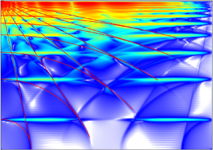
The differences in enstrophy responses in various  $\omega$ ranges noted in figure 3 correspond to distinct spatial features in the enstrophy density
  $|\boldsymbol {\omega }|^{2}$. Figure 4 shows snapshots of
  $E|\boldsymbol {\omega }|^{2}$, for
  $E=10^{-8}$, at the zero phase of the librational forcing for a selection of forcing half-frequencies
  $0<\omega <1$. The first three columns show
  $E|\boldsymbol {\omega }|^{2}$ in the two meridional planes,
  $y=z$ and
  $x=0$, and the equatorial plane,
  $y=-z$. The fourth column shows these planes in the cube with the three-dimensional perspective view corresponding to the schematic in figure 2. The fifth column shows
  $E|\boldsymbol {\omega }|^{2}$ at zero phase on the surface of the cube.

Figure 4. Snapshots of  $E|\boldsymbol {\omega }|^{2}$ at zero phase of the librational forcing on interior planes and on the cube surface (see figure 2 for plane orientations), for
  $E=10^{-8}$ and
  $\omega$ as indicated. Supplementary movie 1 available at https://doi.org/10.1017/jfm.2022.639 shows animations of these over one libration period,
  $\tau ={\rm \pi} /\omega$.
In the  $y=z$ meridional plane, the enstrophy density exhibits characteristics one could anticipate from a purely two-dimensional flow in a container of aspect ratio 1 :
  $\sqrt {2}$, with the rotation axis through the centre and pointing vertically. The linear dispersion relation,
  $\omega ^{2}=\sin ^{2}\theta$, determines the angle
  $\theta$ between the characteristics and the rotation axis. At
  $\omega =1/\sqrt {3}\approx 0.58$, the characteristics emanating from the corners of the rectangular cross-section retrace from diagonally opposite corners. For smaller
  $\omega$, the angle
  $\theta$ becomes smaller and the characteristics emanating from corners reflect off the top and bottom (polar) edges multiple times. The enstrophy density is concentrated along the characteristics. In contrast, for
  $\omega >0.58$, the enstrophy density is no longer concentrated along the characteristics, but instead the characteristics delineate regions of near constant enstrophy density. In addition, in this
  $\omega$-regime, horizontal bands of concentrated enstrophy are also present and become dominant as
  $\omega \to 1$. These bands are not a two-dimensional phenomenon. From the other meridional plane,
  $x=0$, these bands are seen to correspond to other inertial planar wavebeams that intersect the
  $y=z$ meridional plane.
The meridional plane  $x=0$ has aspect ratio 1 : 1, with the axis of rotation being vertical and passing through the centre as well as two corners, corresponding to the midpoints of the two polar edges of the cube at
  $y=z=\pm 0.5$. The sides of this meridional plane make angles
  $\pm {45}^{\circ }$ with the rotation axis. At
  $\omega =1/\sqrt {2}\approx 0.71$, characteristics emanating from the corners are oriented along the sides of the plane. For
  $\omega >0.71$, characteristics from the equatorial corners penetrate into the interior along directions forming the angle
  $\theta$ with the rotation axis consistent with the dispersion relation; these eventually focus into the polar corners following multiple reflections. On the other hand, for
  $\omega <0.71$, the characteristics emanate from the polar corners and tend to focus into the equatorial corners. The intensity of the enstrophy density increases upon each reflection off the walls, which are oblique to the rotation axis. Perhaps unexpectedly from a two-dimensional perspective, the focusing and intensification of the enstrophy density into the equatorial corners is not present in this plane at very low
  $\omega$. There are additional features of the enstrophy density in this plane associated with the three-dimensionality of the flow. For example, at
  $\omega =0.33$, there appear to be two sets of inertial wavebeams emanating from the polar corners, only one of which corresponds to the characteristic directions in that plane. At
  $\omega =0.58$,
  $0.71$ and
  $0.82$, different regions of enstrophy density levels are delimited by curves that appear to be hyperbolic. There is also a vertical line along the rotation axis between the poles, whose intensity depends on
  $\omega$.
The three-dimensional nature of the enstrophy density can be further clarified by considering the equatorial plane,  $y=-z$, in the third column of figure 4. In this view, the rotation axis is orthogonal to the plane and passes through the centre. At frequencies
  $\omega \gtrsim 0.58$ the dominant features are circular shapes together with a horizontal line through the axis. The circular shapes correspond to orthogonal cuts through conical inertial wavebeams emanating from polar vertices above and below the equatorial plane
  $y=-z$, whose intersections with the
  $x=0$ meridional plane produced the observed hyperbolic curves. The horizontal line is coplanar with the vertical line observed in the
  $x=0$ meridional plane, both of which are in the
  $y=z$ meridional plane. At
  $\omega =1/\sqrt {3}\approx 0.58$, the intersection of the four conical beams with the equatorial plane results in two semi-circles which exactly meet at the origin
  $(0,0,0)$. The radius of these circular sections in the equatorial plane is approximately
  $\tan (\theta )/\sqrt {2}=\omega /\sqrt {2(1-\omega ^{2})}$. In particular, this radius is approximately
  $0.25$,
  $0.5$,
  $0.71$ and
  $1$ at
  $\omega =0.33$,
  $0.58$,
  $0.71$ and
  $0.82$, respectively. At low values of
  $\omega$, the conic beams have small aperture resulting in many reflections that intersect the equatorial plane along circular arcs. At
  $\omega =1/\sqrt {2}\approx 0.71$, the conical beams in the equatorial plane touch the equatorial edges (the top and bottom in the planar view). For
  $\omega >1/\sqrt {2}$, the planar beams emanating from the polar edges, that were already observed in the
  $x=0$ meridional plane, intersect the equatorial plane as they reflect on the oblique walls and focus on the equatorial edges. As
  $\omega$ is reduced, the intensification of the enstrophy density associated with the successive reflections of the beams at the oblique walls is strongly biased towards the vertices of the cube at
  $(x,y,z)=(0.5,-0.5,0.5)$ and
  $(-0.5,0.5,-0.5)$. This bias is responsible for the lack of focusing in the
  $x=0$ meridional plane as well as an intricate foliated pattern that radiates out from these two vertices.
The invariance of the flow to the symmetries  $\mathcal {R}$ and
  $\mathcal {S}$ amounts to left–right and up–down reflection symmetries of
  $E|\boldsymbol {\omega }|^{2}$ in the meridional planes
  $y=z$ and
  $x=0$, but only centrosymmetry
  $\mathcal {C}$ in the equatorial plane
  $y=-z$. Column four of figure 4, labelled ‘interior’, shows a three-dimensional perspective view of the enstrophy density in the meridional and equatorial planes, making it easier to reconcile the various traces of planar and conical beams. The symmetry
  $\mathcal {S}$ about the equatorial plane can also be observed on the surface plots of the enstrophy density, shown in column five of figure 4, between the planes
  $y=-0.5$ (top side of cube) and
  $z=0.5$ (right side).
The scaled enstrophy density,  $E|\boldsymbol {\omega }|^{2}$, on the surface of the cube dominates that in the interior by orders of magnitude (note the difference in the colour scales). The predominance of cyan shades indicates that large swathes of enstrophy density with
  $E|\boldsymbol {\omega }|^{2}\sim 1$ form on the surface. This is especially noticeable at
  $\omega =0.71$. At this
  $\omega$, in accord with the dispersion relation, the wavebeams carrying enstrophy are emitted essentially tangentially to the walls and have strong interactions with the boundary layers.
All of the description of flows so far have been of a particular snapshot in time. However, these librationally forced flows are time periodic and, to appreciate this, supplementary movie 1 animates the flows shown in figure 4 over a libration period  $\tau ={\rm \pi} /\omega$. The enstrophy density response in the meridional and equatorial planes are dominated by standing inertial wavebeams. In contrast, the enstrophy density response on the surface shows a distinct progressive wave travelling in the retrograde direction, akin to a Rossby wave resulting from the variable axial distance between the bounding walls (Davidson Reference Davidson2013, chapter 3.5). A similar retrograde wave was also observed in Wu et al. (Reference Wu, Welfert and Lopez2020). Such a wave persists in simulations at
  $\omega >1$ (not shown).
The surface enstrophy density plots at the lower frequencies,  $\omega \lesssim 0.05$, show a focusing of inertial beams into the vertex at
  $(x,y,z)=(0.5,-0.5,0.5)$ and its centro-symmetric counterpart at
  $(-0.5,0.5,-0.5)$, with a distinct foliated pattern. The corresponding interior cross-sectional plots show that this pattern penetrates into the interior of the cube, with a shape which is almost invariant in the direction of the axis of rotation, as is to be expected in the low-frequency regime. Supplementary movie 1 shows that this pattern is also a progressive wave. As
  $\omega$ is increased, the interior cross-sections show a pattern of lines, with focusing shifting from the two equatorial vertices to the equatorial edges for
  $\omega \gtrsim 0.29$, then to the polar edges for
  $\omega \gtrsim 0.71$, with a more uniform response on the surface.
4. Vertex and edgebeam analysis (VEBA)
In this section, we examine to what extent the features of the flows computed at small Ekman number and small libration forcing amplitude,  $E=\epsilon =10^{-8}$, can be captured from linear inviscid considerations.
The librational forcing leads to interactions between boundary layers at contiguous faces resulting in inertial wavebeams being emitted from the vertices and edges of the cube. In the limits of small  $E$ and small
  $\epsilon$, these beams are well described by circularly polarized monochromatic waves with (scaled) velocity
 \begin{equation} \boldsymbol{v} = \boldsymbol{a}\sin\varphi+\boldsymbol{b}\cos\varphi, \end{equation}
where  $\varphi =\boldsymbol {k}\boldsymbol {\cdot }\boldsymbol {x}-2\omega t$,
  $\omega$ is the libration half-frequency,
  $\boldsymbol {k}$ is the wavevector and
  $\boldsymbol {b}=\pm \boldsymbol {a}\times \hat {\boldsymbol {k}}$, where
  $\hat {\boldsymbol {k}}=\boldsymbol {k}/|\boldsymbol {k}|$. The ansatz
  $\boldsymbol {v}$ is a solution of the unforced nonlinear Euler equations, i.e. (2.7a,b) with
  $E=0$ and
  $\omega =0$ (Wu et al. Reference Wu, Welfert and Lopez2020, Appendix A). Note that for this
  $\boldsymbol {v}$, the nonlinear term
  $(\boldsymbol {v}\boldsymbol {\cdot }\boldsymbol {\nabla })\boldsymbol {v}=0$, so that (4.1) is a solution of the unforced equations (free response) for any value of the non-dimensional forcing amplitude
  $\epsilon$.
The energy propagates in the group velocity direction,
 \begin{equation} \hat{\boldsymbol{a}}=\boldsymbol{a}/|\boldsymbol{a}| ={\pm}(1-\omega^{2})^{{-}1/2}\left[\hat{\boldsymbol{\xi}} -(\hat{\boldsymbol{\xi}}\boldsymbol{\cdot}\hat{\boldsymbol{k}})\,\hat{\boldsymbol{k}}\right], \end{equation}
where  $\hat {\boldsymbol {\xi }}$ is the unit vector in the direction of the rotation axis, with
  $\hat {\boldsymbol {a}}\perp \hat {\boldsymbol {k}}$ due to incompressibility. The dispersion relation (Wu et al. Reference Wu, Welfert and Lopez2020, equation (4.6)),
 \begin{equation} (\hat{\boldsymbol{\xi}}\boldsymbol{\cdot}\hat{\boldsymbol{a}})^{2}=1-\omega^{2}, \end{equation}
guarantees that the wave (4.1) solves the unforced inviscid problem. The relation (4.2) can be inverted to recover the wavevector from  $\hat {\boldsymbol {a}}$
 \begin{equation} \hat{\boldsymbol{k}} ={\pm}\omega^{{-}1}\left[\hat{\boldsymbol{\xi}} -(\hat{\boldsymbol{\xi}}\boldsymbol{\cdot}\hat{\boldsymbol{a}})\,\hat{\boldsymbol{a}}\right], \end{equation}
so that  $\hat {\boldsymbol {\xi }}\boldsymbol {\cdot }\hat {\boldsymbol {k}}=\pm \omega$ (Wu et al. Reference Wu, Welfert and Lopez2020, equation (4.2)).
The dispersion relation (4.3) restricts the half-frequency to the inertial range,  $0<\omega <1$, and defines a double cone of rays with directions
 \begin{equation} \hat{\boldsymbol{a}}_\pm = \pm\cos\theta\,\hat{\boldsymbol{\xi}}+\sin\theta\left(\cos\phi\, \hat{\boldsymbol{e}}_x+\sin\phi\, \hat{\boldsymbol{\xi}}\times\hat{\boldsymbol{e}}_x\right), \end{equation}
parameterized by the angle  $-{\rm \pi} <\phi \leqslant {\rm \pi}$, measuring the departure from the direction
  $\hat {\boldsymbol {e}}_x$ of the projection of the beam onto the plane orthogonal to the axis of rotation. In the present problem,
  $\hat {\boldsymbol {\xi }}=(0,1,1)/\sqrt {2}$,
  $\hat {\boldsymbol {e}}_x=(1,0,0)$,
  $\sin \theta =\omega$ and
  $\cos \theta =\sqrt {1-\omega ^{2}}$, with
  $0<\theta <{\rm \pi} /2$. The values of
  $\pm$ and
  $\phi$ depend on
  $\omega$ (i.e.
  $\theta$) and the location and nature of the source of the wave, in particular whether the source is a point or a line.
Each of the eight vertices of the cube acts as a point source from which the energy may propagate into the fluid interior along any ray,  $\hat {\boldsymbol {a}}_\pm$, over an appropriate range of angles,
  $\phi$, that depends on the forcing half-frequency,
  $\omega$. This range can be identified by considering the signs of the three components in the
  $(x,y,z)$ frame of
 \begin{equation} \sqrt{2}\, \hat{\boldsymbol{a}}_\pm = (\sqrt{2}\sin\theta\cos\phi, \pm\cos\theta+\sin\theta\sin\phi, \pm\cos\theta-\sin\theta\sin\phi). \end{equation}
For example, beams emanating from the polar vertex  $\upsilon _1$, at
  $(x,y,z)=(-0.5,-0.5,-0.5)$, must have all three components positive in order to propagate inside the cube, yielding the conditions
  $\pm =+$,
  $\cos \phi >0$ and
  $|\sin \phi |<\textrm {cot}\,\theta =\sqrt {1-\omega ^{2}}/\omega$, i.e.
  $|\phi |<\alpha$ with
  $\alpha ={\rm \pi} /2$ for
  $\omega \leqslant 1/\sqrt {2}$ and
  $\alpha =\arcsin (\sqrt {1-\omega ^{2}}/\omega )$ for
  $\omega >1/\sqrt {2}$. Thus, beams originating at
  $\upsilon _1$ propagate in the interior in directions
  $\hat {\boldsymbol {a}}_+$ for
  $|\phi |<\alpha$. The other three polar vertices in the plane
  $z=y$, labelled
  $\upsilon _2$,
  $\upsilon _3$ and
  $\upsilon _4$, also emit beams in direction
  $\hat {\boldsymbol {a}}_+$ or
  $\hat {\boldsymbol {a}}_-$ into the interior over the whole inertial range. On the other hand, the equatorial vertices in the plane
  $z=-y$, labelled
  $\upsilon _5$,
  $\upsilon _6$,
  $\upsilon _7$ and
  $\upsilon _8$, only emit into the interior of the cube for
  $\omega >1/\sqrt {2}$, but in both
  $\hat {\boldsymbol {a}}_+$ and
  $\hat {\boldsymbol {a}}_-$ directions. The directions of the emitted beams and the corresponding range of
  $\phi$ of the vertex beams associated with the eight vertices are summarized in table 1.
Table 1. Direction of beams emitted in the fluid from each of the eight vertices of the cube over the indicated range of forcing half-frequency  $\omega$. For
  $\omega \leqslant d$,
  $\alpha ={\rm \pi} /2$ and for
  $\omega >d$,
  $\alpha =\arcsin (\sqrt {1-\omega ^{2}}/\omega )$, where
  $d=1/\sqrt {2}$.

The twelve edges of the cube act as line sources. Points on an edge emit beams in parallel directions  $\hat {\boldsymbol {a}}_\pm (\phi )$ that form planar vortex sheets tangent to the conic vortex sheets emanating from the endpoints of the edge, i.e. the associated vertices. This tangentiality condition determines the specific angle
  $\phi$ of the edgebeams in (4.5). The details of how this direction is determined are provided in Appendix A. The resulting direction is consistent with the time-reversal symmetry of the inviscid equations,
 \begin{equation} \mathcal{T}_r: [u,v,w](x,y,z,t)\mapsto[{-}u,-w,-v](x,z,y,-t). \end{equation}
Note that (4.7) is the same symmetry invoked in Wu et al. (Reference Wu, Welfert and Lopez2020) for the case with  $\hat {\boldsymbol {\xi }}=(1,1,1)/\sqrt {3}$ to determine the direction of beams emanating from edges. In both that case and the present case with
  $\hat {\boldsymbol {\xi }}=(0,1,1)/\sqrt {2}$, the
  $y$ and
  $z$ components of
  $\hat {\boldsymbol {\xi }}$ are equal.
Once emitted, the beams eventually reflect on faces, edges or vertices of the cube. A reflected beam is also circularly polarized, with (scaled) velocity
 \begin{equation} \boldsymbol{v}^{\prime} = \boldsymbol{a}^{\prime}\sin\varphi^{\prime}+\boldsymbol{b}^{\prime}\cos\varphi^{\prime}, \end{equation}
where  $\varphi ^{\prime }=\boldsymbol {k}^{\prime }\boldsymbol {\cdot }\boldsymbol {x}-2\omega ^{\prime } t$,
  $\omega ^{\prime }=\pm \omega$ and
  $\boldsymbol {b}^{\prime }=\pm \boldsymbol {a}^{\prime }\times \widehat {\boldsymbol {k}^{\prime }}$. The relation between incident and reflected wavevectors,
  $\boldsymbol {k}$ and
  $\boldsymbol {k}^{\prime }$, follows criteria originally articulated by Phillips (Reference Phillips1963) and recently expressed in vectorial form by Wu et al. (Reference Wu, Welfert and Lopez2020), namely
 \begin{equation} \boldsymbol{k}^{\prime} = \boldsymbol{k}-2s|\boldsymbol{k}|\hat{\boldsymbol{n}}, \end{equation}
where  $\hat {\boldsymbol {n}}$ denotes the normal vector to the reflected surface and
 \begin{equation} s=(\rho-\lambda)/(1-\lambda^{2}), \quad \rho=\hat{\boldsymbol{k}}\boldsymbol{\cdot}\hat{\boldsymbol{n}}, \quad \lambda=(\hat{\boldsymbol{\xi}}\boldsymbol{\cdot}\hat{\boldsymbol{n}})/ (\hat{\boldsymbol{\xi}}\boldsymbol{\cdot}\hat{\boldsymbol{k}}). \end{equation}
The reflection law (4.9) is in general non-Euclidean,  $s\ne \rho$. However, for reflections on faces parallel to the axis of rotation, whose normal vector
  $\hat {\boldsymbol {n}}$ is orthogonal to
  $\hat {\boldsymbol {\xi }}$,
  $\lambda =0$,
  $s=\rho$ and the reflection obeys standard Euclidean laws. This is the case here for reflections on the faces of the cube at
  $x=\pm 0.5$. Similarly, for reflections on a surface with
  $\hat {\boldsymbol {n}}=\pm \hat {\boldsymbol {\xi }}$, the reflection is also Euclidean, with
  $\lambda =1/\rho$ and
  $s=\rho$. This is the case here for reflections on the polar edges at
  $y=z=\pm 0.5$ (
 $e_9$ and
  $e_{10}$ in table 2), using an averaging process to regularize the definition of the normal vector,
  $\hat {\boldsymbol {n}}$, for reflections on edges or vertices, as described in Wu et al. (Reference Wu, Welfert and Lopez2020).
Table 2. Direction of beams emitted in the fluid from points on each of the twelve edges of the cube over the indicated  $\omega$-range. Here,
  $d=1/\sqrt {2}$ and
  $\beta =\textrm {arcsin}(\omega /\sqrt {1-\omega ^{2}})$.

The direction of propagation of the reflected beam's energy is
 \begin{equation} \widehat{\boldsymbol{a}^{\prime}} = \boldsymbol{a}^{\prime}/|\boldsymbol{a}^{\prime}| ={\pm}(1-\omega^{2})^{{-}1/2}\,\left(\hat{\boldsymbol{\xi}} -(\hat{\boldsymbol{\xi}}\boldsymbol{\cdot}\widehat{\boldsymbol{k}^{\prime}}) \widehat{\boldsymbol{k}^{\prime}}\right). \end{equation}
Combining (4.4), (4.9) and (4.11), together with (4.10a–c), leads to the expression
 \begin{equation} \widehat{\boldsymbol{a}^{\prime}} ={\pm}\frac{[(\hat{\boldsymbol{\xi}}\boldsymbol{\cdot}\hat{\boldsymbol{n}})^{2}-\omega^{2}] \hat{\boldsymbol{a}}+ 2(\hat{\boldsymbol{a}}\boldsymbol{\cdot}\hat{\boldsymbol{n}})[\omega^{2}\,\hat{\boldsymbol{n}} -(\hat{ \boldsymbol{\xi}}\boldsymbol{\cdot}\hat{\boldsymbol{n}})\hat{\boldsymbol{\xi}}] } {(\hat{\boldsymbol{\xi}}\boldsymbol{\cdot}\hat{\boldsymbol{n}})^{2}-\omega^{2}- 2(\hat{\boldsymbol{a}}\boldsymbol{\cdot}\hat{\boldsymbol{n}}) (\hat{\boldsymbol{n}}\boldsymbol{\cdot}\hat{\boldsymbol{\xi}}) (\hat{\boldsymbol{\xi}}\boldsymbol{\cdot}\hat{\boldsymbol{a}})}, \end{equation}
in terms of the incident vector  $\hat {\boldsymbol {a}}$, with
  $\hat {\boldsymbol {\xi }}\boldsymbol {\cdot }\hat {\boldsymbol {a}}$ and
  $\omega$ obeying the dispersion relation (4.3). In particular, the direction of
  $\hat {\boldsymbol {a}}^{\prime }$ is independent of the orientation of
  $\hat {\boldsymbol {a}}$,
  $\hat {\boldsymbol {\xi }}$ or
  $\hat {\boldsymbol {n}}$. The ratio
 \begin{equation} |\boldsymbol{a}^{\prime}|/|\boldsymbol{a}| = |\boldsymbol{k}^{\prime}|/|\boldsymbol{k}| = |\alpha|, \end{equation}
where
 \begin{equation} \alpha=1-2\lambda s=(1-2\rho\lambda+\lambda^{2})/(1-\lambda^{2}), \end{equation}
determines the change of wavelength upon reflection (Wu et al. Reference Wu, Welfert and Lopez2020, equations (4.21) and (4.18)). Note that (4.14) is independent of the orientation of  $\hat {\boldsymbol {\xi }}$,
  $\hat {\boldsymbol {k}}$ or
  $\hat {\boldsymbol {n}}$. For Euclidean reflections,
  $\alpha =1$ (
 $\lambda =0$) or
  $\alpha =-1$ (
 $\rho \lambda =1$), and the beam's enstrophy density,
  $|\boldsymbol {\omega }|^{2}$, remains unchanged. Otherwise, the ratio of reflected to incident enstrophy densities is
 \begin{equation} |\boldsymbol{\omega}^{\prime}|^{2}/|\boldsymbol{\omega}|^{2}= |\boldsymbol{a}^{\prime}|^{2}|\boldsymbol{k}^{\prime}|^{2}/|\boldsymbol{a}|^{2}|\boldsymbol{k}|^{2}= \alpha^{4}. \end{equation}
For  $|\alpha |>1$, there is a decrease in the wavelength (focusing) and an increase in the beam's enstrophy density upon reflection.
In the configuration currently being studied, with  $\hat {\boldsymbol {\xi }}=(0,1,1)/\sqrt {2}$, the cube's faces at
  $x=\pm 0.5$ are parallel to the rotation axis, with
  $\lambda =0$, on which reflections are Euclidean. The other four faces are inclined at
  $\pm {45}^{\circ }$ to the rotation axis, with
  $\lambda ^{2}=1/(2\omega ^{2})$ and the reflections are not Euclidean. There are essentially two VEBA regimes for this configuration. In one regime,
  $\omega <1/\sqrt {2}$ and
  $|\lambda |>1$, the beams are emitted from the four polar vertices in the meridional plane
  $y=z$,
  $\upsilon _i$ (
 $1\leqslant i\leqslant 4$), and from any of the ten non-polar edges,
  $e_i$ (
 $1\leqslant i\leqslant 10)$. These beams reflect on the faces of the cube and focus on the equatorial edges,
  $e_{11}$ and
  $e_{12}$. This is illustrated in figure 5(a–d) for
  $\omega =0.33$, with vortex sheets emanating from
  $\upsilon _1$ as well as several edges. The reflections are supercritical on the four faces that are inclined to the rotation axis and Euclidean on the other two faces. In the other regime, with
  $\omega >1/\sqrt {2}$ and
  $|\lambda |<1$, beams are emitted from all eight vertices
  $\upsilon _i$ (
 $1\leqslant i\leqslant 8$), but only from the two equatorial edges,
  $e_{11}$ and
  $e_{12}$. This is illustrated in figure 5(e–g) for
  $\omega =0.82$, with vortex sheets emanating from
  $\upsilon _1$ and equatorial edge
  $e_{11}$. Following subcritical reflections on the inclined faces of the cube and Euclidean reflections on the other two faces, the beams focus on the polar edges
  $e_9$ or
  $e_{10}$. An illustration of reflection criticality is provided in Wu et al. (Reference Wu, Welfert and Lopez2020, figure 7).

Figure 5. The VEBA at half-frequencies (a–d)  $\omega =0.33$ and (e–g)
  $\omega =0.82$, showing
  $10^{-8}\alpha ^{4}$, with beams emitted with enstrophy density
  $\alpha ^{4}=10$. (a) Conic vortex sheet emanating from the polar vertex
  $\upsilon _1$ reflected onto the walls of the cavity and focusing onto equatorial edges
  $e_{11}$ and
  $e_{12}$; (b–d) planar vortex sheets emanating from edges
  $e_{10}$,
  $e_7$ and
  $e_8$, respectively. (e) Conic vertex sheet emanating from
  $\upsilon _1$ and focusing onto edge
  $e_{10}$. (f) Conic vertex sheet emanating from
  $\upsilon _5$ focusing onto edges
  $e_9$ and
  $e_{10}$. (g) Planar vortex sheets emanating from edge
  $e_{11}$.
The explicit determination of the traces of the conic vortex sheet emanating from vertex  $\upsilon _1$, the planar vortex sheet emanating from edge
  $e_1$ and their reflections in the equatorial plane is included in Appendix B. These traces consist of arcs of circles and segments of lines which form, at low
  $\omega$, a criss-crossing pattern whose geometric characteristics are also described in Appendix B.
In both cases, the ratio (4.14), quantifying the change in the beam's energy upon reflection, tends to a limit
 \begin{equation} \alpha_\infty= \frac{1+2\sqrt{\omega^{2}(1-\omega^{2})}}{2\omega^{2}-1}= \frac{\omega+\sqrt{1-\omega^{2}}}{\omega-\sqrt{1-\omega^{2}}}={-}\text{cot}\left(\frac{\rm \pi}{4}-\theta\right), \end{equation}
obtained by applying a result from Wu et al. (Reference Wu, Welfert and Lopez2020, equation (C7)). Note that (4.16) is real over the whole inertial frequency range,  $0<\omega <1$, with
  $|\alpha _\infty |>1$. Also, the asymptotic rate of increase of the wave speed,
  $\alpha _\infty$, is related to the geometric rate of focusing,
  $\gamma =-1/\alpha _\infty$, see (B2). In contrast, the corresponding expression in Wu et al. (Reference Wu, Welfert and Lopez2020, equation (4.25)), resulting from the substitution
  $\omega ^{2}\to 3\omega ^{2}/2$ in (4.16), for libration around an axis
  $(1,1,1)/\sqrt {3}$ passing through opposite vertices of the cube, for which
  $\alpha _\infty$ becomes complex in the range
  $\sqrt {2/3}<\omega <1$, with focusing towards polar vertices. This analogy suggests that the focusing to equatorial vertices observed in the present configuration in the low-
 $\omega$ regime may be a consequence of viscous effects, which create a detuning
  $\omega ^{2}\to \omega ^{2}-\omega _0^{2}$, and the complexification of (4.16) for
  $0<\omega <\omega _0$. This conjecture is supported by the sequence of interior cross-sections of
  $E|\boldsymbol {\omega }|^{2}$ obtained at small Ekman number,
  $E=10^{-8}$, shown in figure 4, with focusing shifting from the equatorial vertices to the equatorial edges.
5. Comparison of inviscid predictions and Navier–Stokes simulations
In the VEBA framework, the enstrophy density is time invariant. As such, it is more appropriate to compare the enstrophy density from VEBA with the time-averaged enstrophy density of the forced response from the Navier–Stokes simulations (direct numerical simulations, DNS) at the smallest values of Ekman number and librational forcing amplitude available, namely  $E=\epsilon =10^{-8}$. The scaled time-averaged enstrophy density,
  $E\overline {|\boldsymbol {\omega }|^{2}}$, for the same forcing half-frequencies
  $\omega$ and planar views as in figure 4, showing snapshots of
  $E|\boldsymbol {\omega }|^{2}$ at the zero phase of the librational forcing, are shown in figure 6. The corresponding view of the enstrophy density from VEBA are shown in figure 7. While VEBA dictates the change in enstrophy density upon reflections, the value of the enstrophy density of the emitted beams is arbitrary and was set to
  $|\boldsymbol {\omega }|^{2}=10$ in figure 7 to visually match the DNS results. The regularization of the normal direction at the polar edges,
  $e_9$ and
  $e_{10}$, results in only Euclidean reflections in the meridional plane
  $y=z$. As a consequence, beams emanating in this plane remain at a fixed energy level upon reflections, and tend to fill the plane after many reflections. In order to match the DNS, a dissipation factor of
  $\sqrt {1-\omega ^{2}}$ is introduced into the VEBA at the polar edges. This is implemented by replacing
  $\alpha$ from (4.14) with
  $\alpha \sqrt {1-\omega ^{2}}$ for reflections at the polar edges. The
  $\sqrt {1-\omega ^{2}}$ factor is not needed for the other two planes visualized in the figure,
  $x=0$ or
  $y=-z$, because beams that solely reside in these planes focus into edges.

Figure 6. Scaled time-averaged enstrophy,  $E\overline {|\boldsymbol {\omega }|^{2}}$, over one period of the librational forcing on interior planes and on the cube surface (see figure 2 for plane orientations), for
  $E=10^{-8}$ and
  $\omega$ as indicated.

Figure 7. The VEBA of  $10^{-8}|\boldsymbol {\omega }|^{2}$ on interior planes and of
  $10^{-4}|\boldsymbol {\omega }|^{2}$ on the cube surface (see figure 2 for plane orientations), for
  $\omega$ as indicated. All beams are emitted with intensity
  $|\boldsymbol {\omega }|^{2}=10$.
There is overall good agreement between the DNS and VEBA both in the interior and the surface, particularly, the sharp maxima of enstrophy density in the DNS. For  $\omega \gtrsim 0.58$, the interior enstrophy density in the DNS has regions of approximately piecewise constant intensity. These regions are demarcated by surfaces corresponding to vortex sheets emanating from vertices and edges which are captured by the VEBA. These were also observed in the librating cube oriented with
  $\hat {\boldsymbol {\xi }}=(1,1,1)/\sqrt {3}$, shown in figure 1(b), but not fully appreciated at the time (Wu et al. Reference Wu, Welfert and Lopez2020). Analogous low-regularity solutions were studied in considerable detail in a stratified flow subjected to periodic horizontal forcing (Grayer et al. Reference Grayer, Yalim, Welfert and Lopez2021).
Another difference between DNS and VEBA is their symmetry; VEBA is an analysis of the inviscid system and has symmetries  $\mathcal {R}$ and
  $\mathcal {S}$ of the full Navier–Stokes system (2.7a,b), as well as the time-reversal symmetry
  $\mathcal {T}$ (4.7). The viscous terms in the full system (2.7a,b) are not invariant to
  $\mathcal {T}$. This difference in symmetries becomes more pronounced as
  $\omega \to 0$, particularly in the equatorial plane
  $y=-z$. Figure 8 shows snapshots at the zero phase of the librational forcing of the enstrophy density in the equatorial plane
  $y=-z$ from DNS responses at Ekman numbers ranging from
  $E=10^{-5}$ to
  $10^{-8}$ and decreasing forcing half-frequency, starting from
  $\omega =0.16$. The figure can be viewed as an array with columns corresponding to fixed values of
  $\omega$, with
  $\omega$ halved in each column to the right, and rows corresponding to fixed
  $E$, with
  $E$ reduced by one order of magnitude in each subsequent row. For fixed
  $\omega$, the patterned vortex structure emanating from the two equatorial vertices,
  $\upsilon _6$ and
  $\upsilon _7$, and already observed at
  $\omega =0.05$ and
  $\omega =0.20$ in figure 4, eventually develops from the faces at
  $x=\pm 0.5$ at sufficiently low
  $E$ for all
  $\omega$ in the range considered in the figure. The extent and intensity of the foliation pattern remain similar along diagonals of the array with the foliations becoming finer with a higher motif count varying approximately inversely proportionally with
  $\omega$ as
  $E$ and
  $\omega$ decrease to
  $0$. At
  $E=10^{-8}$, the DNS at
  $\omega =0.16$ is well described by VEBA, but not for smaller
  $\omega$. The similarity in the DNS along diagonals in the array then allows one to extrapolate how small
  $E$ needs to be at smaller
  $\omega$ for agreement between DNS and VEBA:
  $\omega =0.01$ is four columns to the right of the
  $\omega =0.16$ column, so the
  $E$ for its DNS to be matched by VEBA should be four rows below the
  $E=10^{-8}$ row, giving
  $E=10^{-12}$. From figure 3(d), we also have that
  $E\bar {\mathcal {E}}\sim \omega ^{2}$ is independent of
  $E$ in the limit
  $\omega \to 0$. Moving along the diagonal in figure 8,
  $\omega$ varies with
  $E^{0.3}$ (where
  $0.3\approx \log _2 10$). As a result,
 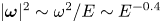 $|\boldsymbol {\omega }|^{2}\sim \omega ^{2}/E \sim E^{-0.4}$.

Figure 8. Snapshots of  $E|\boldsymbol {\omega }|^{2}$ at the zero phase of the librational forcing in the equatorial plane,
  $y=-z$, for
  $\omega$ and
  $E$ as indicated. The bottom row shows the corresponding VEBA of
  $10^{-8}|\boldsymbol {\omega }|^{2}$. Supplementary movie 2 animates these over one libration period,
  $2{\rm \pi} /\omega$.
The foliated pattern remains intact while gaining strength as  $E$ decreases, before eventually being sliced up by the network of planar and conic wavebeams associated with reflections of the beams emanating from polar edges and vertices, resulting in an increasingly denser pattern of horizontal (cyan/yellow) lines and arcs for the enstrophy density response in the equatorial plane. However, this slicing extends in the equatorial plane only up to some distance away from the equatorial edges, which progressively decreases with decreasing
  $E$ at fixed
  $\omega$, and ultimately vanishes in VEBA. The apparent lack of convergence of the exponent
  $\alpha _\mathcal {K}$ in the power law of
  $\mathcal {K}$ in the low-
 $\omega$ regime as
  $E$ is reduced down to
  $10^{-8}$ observed in figure 3(e) is tied to the presence of the foliation pattern. These are manifestations of viscous effects and nonlinear wave–wave interactions not accounted for in VEBA.
6. Flow velocity
The VEBA provides an excellent description of most features of the response flows from the DNS at sufficiently small  $E$ over the entire inertial range, and in particular for
  $\omega \gtrsim 0.29$, although for DNS at
  $\omega \lesssim 0.29$ there is a clear breaking of the inviscid time-reversal symmetry (4.7). For
  $\omega \approx 0.29$, there is a large spike in the time-averaged kinetic energy response diagram (figure 3a), which becomes more pronounced with decreasing
  $E$ but is not predicted by the linear inviscid VEBA. To further investigate the cause of this, we now consider the velocity flow field from DNS in this
  $\omega$ regime. Figure 9(a) shows snapshots at the zero librational forcing phase of coneplots of the velocity,
  $\boldsymbol {v}$, for
  $E=10^{-8}$ and
  $\omega =0.20$ (associated with the peak time-averaged enstrophy response in figure 3b), and
  $\omega =0.29$ and
  $0.30$ either side of the time-averaged kinetic energy peak. The cones represent the local velocity vectors at Legendre–Lobatto points inside the cube. Their size and colour vary logarithmically with speed
  $|\boldsymbol {v}|$, as indicated by the cones along the colour bar. The dominant cyan colour reflects the size of order
  $1$ of speed in the bulk. Figure 9(b) shows a
  $\times 3$ magnification about the vertex
  $\upsilon _6$ of the same three cases. The magnified view not only allows for more densely spaced velocity cones, but the cuts through the cube also allow clearer views of the velocity cones in the interior.

Figure 9. Snapshots of the velocity  $\boldsymbol {v}$, depicted as coneplots, at zero phase for
  $E=10^{-8}$ and
  $\omega$ as indicated. A full view of the cube is presented in row (a), and row (b) shows
  $\times 3$ magnifications near the vertex
  $\upsilon _6$ at
  $(x,y,z)=(0.5,-0.5,0.5)$ for the same cases as in (a). The cones representing the local velocity vectors are shown at Legendre–Lobatto points inside the cube. Their size and colour vary logarithmically with
  $|\boldsymbol {v}|$. Supplementary movie 3 animates these over one libration period
  ${\rm \pi} /\omega$.
While the snapshots are informative, it is essential to view these velocity cones animated over a complete libration period. This is available in supplementary movie 3. The velocity in the interior is clearly circularly polarized, as assumed by the idealization in the VEBA. The speed is slower near the rotation axis. In contrast, near the cube boundaries the polarization tends to ‘snap’ every half-period, with a much more eccentric elliptic polarization. For  $\omega \lesssim 0.29$ the speed is largest in the foliations around the equatorial vertices
  $\upsilon _6$ and
  $\upsilon _7$ only, which are farthest (together with the other two equatorial vertices
  $\upsilon _5$ and
  $\upsilon _8$) from the rotation axis. For
  $\omega =0.30$ the largest magnitudes have shifted along the equatorial edge(s), with a much lower intensity associated with a sharp drop in the time-averaged kinetic energy
  $\bar {\mathcal {K}}$ in figure 3(a), and a more uniformly circularly polarized velocity
  $\boldsymbol {v}$. As
  $\omega$ increases from
  $0.20$ to
  $0.29$ the vertex of the foliation moves from
  $\upsilon _6$ to a point on the equatorial edge, resulting in a whirlpool around the corner
  $\upsilon _6$, before it suddenly disappears at larger
  $\omega$.
The progressive waves noted from the animations of the enstrophy density in supplementary movie 1 can also be seen in the velocity animations in supplementary movie 3. The boundary progressive wave can now be seen to be associated with the phase of the ‘snapping’. This is true across all frequencies. As well, the foliated pattern noted in the enstrophy density is also present in the velocity animations at the lower  $\omega$. The
  $\times 3$ zoom of the
  $\omega =0.20$ case shows this very clearly in the vicinity of the
  $\upsilon _6$ vertex.
7. Conclusions
In this study, we complete the investigation of the three principal orientations of a fluid-filled rapidly rotating cube subjected to libration – small harmonic-in-time modulation of its rotation rate. The three principal orientations are the rotation axis passing through the middle of two opposite faces, through two opposite vertices, and through the middle of two opposite edges. The orientations each have one of the three types of proper rotation symmetries of the cube. Only the first orientation has been studied experimentally (Boisson et al. Reference Boisson, Lamriben, Maas, Cortet and Moisy2012). Our interests lie principally in a number of limiting regimes. One regime is the fast rotation regime, where the mean rotation period is much smaller than the viscous time scale in the cube. The ratio of these two time scales is the Ekman number,  $E=\varOmega L^{2}/\nu$. Another regime is the small forcing amplitude regime, where the amplitude of the modulation of the rotation,
  $\Delta \varOmega$, is small compared with the mean rotation. The ratio
  $\epsilon =\Delta \varOmega /\varOmega$ is the Rossby number for this class of flows. When
  $E$ and
  $\epsilon$ are both sufficiently small, the flow responses to librational forcing are dominated by inertial oscillations when the libration frequency,
  $\sigma$, is less than twice the mean rotation rate, i.e. for
  $\omega =\sigma /2\varOmega \in (0,1)$. The three limits,
  $E\to 0$,
  $\epsilon \to 0$ and
  $\omega \to 0$, are singular. The
  $E\to 0$ and
  $\epsilon \to 0$ limits are often invoked in unbounded domains to arrive at a linear hyperbolic differential equation describing inertial waves, from which a dispersion relation is obtained (Greenspan Reference Greenspan1968). The
  $\omega \to 0$ limit is invoked to arrive at the Taylor–Proudman theorem (Proudman Reference Proudman1916; Taylor Reference Taylor1917). What happens as each of these limits is approached in a confined setting is not at all obvious, especially when the walls of the container have components of their motion that are not tangential. Further complications arise when any of the walls are oblique to the rotation axis. Our results emphasize that the limits
  $E\to 0$ and
  $\epsilon \to 0$ do not mean that
  $E{\nabla }^{2}\boldsymbol {v}\to 0$ or
  $\epsilon (\boldsymbol {v}\boldsymbol {\cdot }\boldsymbol {\nabla })\boldsymbol {v}\to 0$; these terms may remain
  ${O}(1)$ due to
  $\boldsymbol {v}$ tending to being non-smooth (e.g. a delta function-like distribution) in the
  $E\to 0$ limit. In any case, we find that
  $E=\epsilon =10^{-8}$ is still not asymptotically small and viscous and nonlinear effects are not negligible, particularly as
  $\omega \to 0$.
We are able to conclude that  $E=\epsilon =10^{-8}$ is not asymptotically small from DNS of the fully nonlinear Navier–Stokes equations with no-slip boundary conditions. The global measures, such as the kinetic energy and enstrophy in the cube, are far from reaching an asymptotic limit. Furthermore, setting
  $E=\epsilon =0$ allows one to explore the traces of inertial waves of a given frequency (the so-called VEBA) and compare these with the DNS results at small but finite
  $E$ and
  $\epsilon$. As noted by Rabitti & Maas (Reference Rabitti and Maas2014): ‘Understanding the behaviour of internal waves in fully enclosed domains constitutes one of the big challenges in fluid dynamics…. Since analytical solutions for internal waves in arbitrarily shaped domains are not available, numerical approaches or geometrical ray-tracing techniques have been widely used in order to infer properties of the underlying wavefield and energy distribution in the container’. The VEBA, first developed in Wu et al. (Reference Wu, Welfert and Lopez2020), is not only a ray-tracing technique, but also a ray-emitting exercise that considers not just individual rays, but a collection of rays making up sheets that must satisfy continuity and tangentiality conditions. These conditions allow us to determine where beams are emitted from and their direction into the cube. Not all edges emit wavebeams for all
  $\omega$; it all depends on whether the vertices at the ends of the edges emit into the interior or not. This realization clarifies a long-standing question as to why some edges emit beams while others do not. While VEBA captures an overwhelming majority of the details from the DNS, there remain aspects of the DNS response flows that are not captured, particularly at small
  $\omega$.
Supplementary movies
Supplementary movies are available at https://doi.org/10.1017/jfm.2022.639.
Acknowledgments
The direct numerical simulations were performed on ASU Research Computing and Purdue facilities. K. Wu thanks Professor J. Shen, as well as his co-authors, for guidance with the development and construction of the numerical scheme and computer code used in this study.
Declaration of interests
The authors report no conflict of interest.
Appendix A. The confluence of conical and planar vortex sheets.
Edgebeams emanate from each point of a straight edge in parallel directions  $\hat {\boldsymbol {a}}$, forming a planar vortex sheet that merges smoothly and tangentially with the conic vortex sheets emanating from the endpoints of the straight edge. Thus, the direction individual edgebeams are emitted in from an edge depends on whether the endpoints of the edge are emitting into the cube. There are two scenarios, which are illustrated here for
  $\omega <1/\sqrt {2}$. In the first scenario, both endpoints of the edge emit inside the cube, as is the case for example with edge
  $e_{12}$ connecting vertices
  $\upsilon _7$ and
  $\upsilon _8$ (see figure 10a). Since the conic sheets emanating from both vertices are identical, the planar vortex sheet emanating from the edge has a normal perpendicular to
  $\hat {\boldsymbol {e}}_x$, with beams emitted in planes
  $x=\textrm {const.}$, with
  $\phi =-{\rm \pi} /2$ and
 \begin{align} \hat{\boldsymbol{a}}&=\cos\theta\,\hat{\boldsymbol{\xi}} - \sin\theta\,\hat{\boldsymbol{\xi}}\times\hat{\boldsymbol{e}}_x \nonumber\\ &=\frac{\sqrt{1-\omega^{2}}}{\sqrt{2}}(0,1,1)- \frac{\omega}{\sqrt{2}}(0,1,-1) \nonumber\\ &=\frac{1}{\sqrt{2}}\left(0,-\omega+\sqrt{1-\omega^{2}},\omega+\sqrt{1-\omega^{2}}\right). \end{align}
In the other scenario, only one of the endpoints emits vertex beams into the cube, as is the case for edge  $e_1$ connecting vertices
  $\upsilon _1$ and
  $\upsilon _7$ (see figure 10b). The tangentiality condition of the planar vortex sheet emanating from the edge with the conic sheet emanating from
  $\upsilon _1$ results in beams emitted into the direction
 \begin{align} \hat{\boldsymbol{a}} &=\cos\theta\,\hat{\boldsymbol{\xi}} + \sin\theta\left(\cos\phi\,\hat{\boldsymbol{e}}_x + \sin\phi\,\hat{\boldsymbol{\xi}}\times\hat{\boldsymbol{e}}_x\right)\nonumber\\ &=\frac{\sqrt{1-\omega^{2}}}{\sqrt{2}}(0,1,1) +\omega\left[\frac{\sqrt{1-2\omega^{2}} }{\sqrt{ 1-\omega^{2}}}(1,0,0)+ \frac{\omega}{\sqrt{2(1-\omega^{2})}}(0,1,-1)\right]\nonumber\\ &=\frac{1}{\sqrt{2(1-\omega^{2})}} \left[\omega\sqrt{2(1-2\omega^{2})},1,1-2\omega^{2}\right]. \end{align}
A symmetrically related planar sheet is emitted from edge  $e_2$, as shown in figure 10(b). At
  $\omega =1/\sqrt {2}$, the trace of the conic sheet in the equatorial plane kisses the two edges
  $e_1$ and
  $e_2$. For
  $\omega >1/\sqrt {2}$, the edges
  $e_1$ and
  $e_2$ no longer emit beams in the cube.

Figure 10. Illustration of the tangential confluence of a (green) planar vortex sheets made up of edgebeams with either two or one (red) conic vortex sheet(s) emanating from the endpoints of the edge: (a) edgebeams emanating from edge  $e_9$ for
  $\omega <1/\sqrt {2}$; (b) edgebeams emanating from edge
  $e_1$ for
  $\omega <1/\sqrt {2}$. Other vertex beams are shown in red. In this figure
  $\hat {\boldsymbol {\xi }}$ represents a vector parallel to the axis of rotation.
Appendix B. The geometry of VEBA on the equatorial plane
In order to algebraically describe the traces of the vortex sheets emanating from the vertex  $\upsilon _1$ and the edge
  $e_1$, and of their reflections, in the plane
  $x=-0.5$ and the equatorial plane
  $y=z$, it is convenient to introduce a (negatively oriented) frame
  $(\hat {\boldsymbol {e}}_x,\hat {\boldsymbol {e}}_Y,\hat {\boldsymbol {\xi }})$, with
  $\hat {\boldsymbol {e}}_Y=\hat {\boldsymbol {e}}_x\times \hat {\boldsymbol {\xi }}$ and coordinate system
 \begin{equation} (X,Y,Z)=\left[x+0.5,d(1-y+z),d(y+z)\right], \end{equation}
with its origin at vertex  $\upsilon _7$ at
  $(x,y,z)=(-0.5,0.5,-0.5)$, where
  $d=1/\sqrt {2}$ (see figure 11c). In the plane
  $X=0$, the intersections of the beam emanating from
  $\upsilon _1$, or its
  $k$th reflections, and the equatorial plane
  $Z=0$, occur at points
  $Y=\zeta _k$ (see figure 11a). These intersection points converge to the origin, i.e.
  $\zeta _k \to 0$, geometrically with rate
 \begin{equation} \gamma:=\tan\left(\dfrac{\rm \pi}{4}-\theta\right)=\frac{1-t}{1+t}, \quad\text{where}\ t=\tan\theta=\dfrac{\omega}{\sqrt{1-\omega^{2}}}. \end{equation}
Note that  $|\gamma |<1$ over the whole inertial range,
  $0<\omega <1$, but
  $\gamma >0$ only if
  $0<\omega <1/\sqrt {2}$; this is the frequency range considered here and illustrated for
  $\omega =0.33$ in figure 11. Then
 \begin{equation} \zeta_k = \zeta_{k-1}\,\gamma = \zeta_0\,\gamma^{k}=d(1-t)\,\gamma^{k}. \end{equation}
The quantity  $r=at$ in figure 11(b) is the radius of the (arc of) circle centred at the midpoint between vertices
  $\upsilon _1$ and
  $\upsilon _3$,
  $(X,Y)=(0,c_0)=(0,a)$, and represents the trace of the conic vortex sheet emanating from vertex
  $\upsilon _1$ in the equatorial plane
  $Z=0$. The parameterization of this arc,
 \begin{equation} (X,Y) = (r\cos\phi, d-r\sin\phi), \quad 0\leqslant\phi<{\rm \pi}/2, \end{equation}
describes the intersection with the equatorial plane of the edgebeam emanating from vertex  $\upsilon _1$ in the direction
 \begin{equation} \hat{\boldsymbol{a}}= \frac{X\hat{\boldsymbol{e}}_x + (Y-d)\hat{\boldsymbol{e}}_Y + d\hat{\boldsymbol{\xi}}}{\sqrt{X^{2}+(Y-d)^{2}+d^{2}}} = \cos\theta\,\hat{\boldsymbol{\xi}}+\sin\theta(\cos\phi\,\hat{\boldsymbol{e}}_x -\sin\phi\,\hat{\boldsymbol{e}}_Y), \end{equation}
in agreement with (4.5). The corresponding wavevector  $\boldsymbol {k}$ is obtained from (4.4). The wavebeam then alternately reflects onto the walls at
  $y=0.5$ (i.e.
  $Y-Z=0$) and
  $z=-0.5$ (i.e.
  $Y+Z=0$). At reflection
  $k>0$, the unit vector normal to the reflecting wall is
 \begin{equation} \hat{\boldsymbol{n}}=d[\hat{\boldsymbol{\xi}}-({-}1)^{k}\hat{\boldsymbol{e}}_Y]. \end{equation}
The direction of the reflected beam,  $\hat {\boldsymbol {a}}^{(k)}$, can be obtained from that of the incident beam,
  $\hat {\boldsymbol {a}}^{(k-1)}$, using (4.12) with
  $\pm =(-1)^{k}$ and
  $\hat {\boldsymbol {a}}^{(0)}=\hat {\boldsymbol {a}}$ from (B5). This direction is best expressed in the form
 \begin{equation} \hat{\boldsymbol{a}}^{(k)} = ({-}1)^{k}\cos\theta\,\hat{\boldsymbol{\xi}}+\sin\theta\,\hat{\boldsymbol{e}}^{(k)}, \end{equation}
with
 \begin{equation} \hat{\boldsymbol{e}}^{(k)}(b):=\text{sech}(2ka+b)\,\hat{\boldsymbol{e}}_x -\tanh(2ka+b)\,\hat{\boldsymbol{e}}_Y, \end{equation}
where
 \begin{equation} a := \tanh^{{-}1}(t) \quad\text{and}\quad b := \tanh^{{-}1}(\sin\phi)\in[0,\infty). \end{equation}
The beams intersect the equatorial plane  $Z=0$ at
 \begin{equation} M_k(b):=[X_k(b),Y_k(b)] := (0,c_k)+r_k\,\hat{\boldsymbol{e}}^{(k)}(b), \end{equation}
where
 \begin{equation} r_k := d\,\frac{\sinh(2k+1)a}{\cosh a} \quad\text{and}\quad c_k := d\,\frac{\cosh(2k+1)a}{\cosh a} = r_k+\zeta_k, \end{equation}
and are reflected on the walls  $Z = (-1)^{k}Y$ at the points
 \begin{equation} P_k(b):= d\,\frac{\big[\text{sech}\,a\sinh 2ka,\cosh(a-b), -({-}1)^{k}\cosh(a-b)\big] } { \cosh [ (2k-1)a+b ] } . \end{equation}
The proofs of (B7)–(B8) and (B10)–(B12) are fairly technical and outlined in Appendix C. For  $k=0$, the coordinates (B12) reduce to
  $d[0,1,-1]$, i.e. the coordinates of the vertex
  $\upsilon _1$. Moreover,
  $r_0=d\tanh a=\textrm {d}t=r$,
  $c_0=d$ and (B10) reduces to (B4). Note also that
 \begin{equation} \begin{bmatrix} r_k\\c_k\end{bmatrix} =\begin{bmatrix}\cosh(2ka) & \sinh(2ka) \\ \sinh(2ka) & \cosh(2ka) \end{bmatrix}\begin{bmatrix}r\\ {d} \end{bmatrix}. \end{equation}
Thus, for each  $\phi$ (i.e.
  $b$), the associated wavebeam emanating from
  $P_0(b)$ in the direction
  $\hat {\boldsymbol {a}}^{(0)}$ intersects the equatorial plane at
  $M_0(b)$ and is reflected at
  $P_1(b)$ on the plane
  $Z=Y$ in direction
  $\hat {\boldsymbol {a}}^{(1)}$. The reflected beam intersects the equatorial plane at
  $M_1(b)$ before reflecting on the plane
  $Z=-Y$ at
  $P_2(b)$, and so on.

Figure 11. Geometric construction of VEBA traces for  $\omega =0.33$: (a) in the plane
  $x=-0.5$ the conical wavebeam emanating from
  $\upsilon _1$ towards edge
  $e_4$ at an angle
  $\theta$ with the direction of the axis of rotation is reflected successively onto edges
  $e_4$ and
  $e_1$ at a geometric rate
  $\gamma$; (b) the conical vortex sheet emanating from
  $\upsilon _1$ and its reflections intersect the equatorial plane
  $y=z$ along (red) arcs of circles with centres
  $(0,c_k)$ on the
  $Y$ axis. The endpoints
  $M_k(0)$ corresponding to the reflections of the conical wavebeam emitted in direction
  $\phi =0^{+}$ are themselves located on a quarter circle of radius
  $d=1/\sqrt {2}$ centred at
  $(r,0)$ (bold black arc). The planar vortex sheet emanating from edge
  $e_1$ and its reflections intersect the equatorial plane along (red) line segments tangent to the arcs at points
  $M_k(a)$ on a circle of radius
  $\sqrt {d^{2}-r^{2}}$ centred at
  $\upsilon _7$ (light black arc). Panel (c) shows the three-dimensional orientations of the planes in (a,b).
The parametric equations (B10) represent an arc of circle with centre  $(0,c_k)$ and radius
  $r_k$ (see figure 11b). The extremal points of the arc are
 \begin{equation} M_k(\infty)=(0,c_k-r_k)=(0,\zeta_k), \end{equation}
and, using (B13),
 \begin{align} M_k(0)&= \left[r_k\,\text{sech}(2ka),c_k-r_k\tanh(2ka)\right]\nonumber\\ &=(r,0)+d[\tanh(2ka),\text{sech}(2ka)]. \end{align}
The points  $M_k(0)$, which correspond to the traces in the equatorial plane
  $Z=0$ of the successive reflections of the beam emanating from
  $\upsilon _1$ in the
  $\hat {\boldsymbol {e}}_x$ direction, are on a circle of radius
  $d$ centred at
  $(r,0)$; these are shown in figure 11(b) as a thick black arc. Note that
  $M_0(0)$ is in the meridional plane
  $y=z$. The relations (B15) also show that
 \begin{equation} \frac{c_k-Y_k(0)}{X_k(0)}= \sinh(2ka)=\frac{X_k(0)-r}{Y_k(0)}=:\tan\phi_{2k}, \end{equation}
i.e. the radial line between  $(r,0)$ and
  $M_k(0)$ forms an angle
  $\phi _{2k}$ with the
  $Y$ direction and is tangent to the parametric curve (B10) at
  $M_k(0)$.
From Appendix A, the planar edgebeam emanating from the edge  $e_1$ connecting the vertices
  $\upsilon _1$ and
  $\upsilon _7$ is tangent to the conic vertex beam emanating from
  $\upsilon _1$, as are their cross-sections in the equatorial plane. The trace of the edgebeam passes through the origin,
  $(X,Y)=(0,0)$, and is tangent to the circle of radius
  $r$ centred at
  $(0,d)$, at a point associated with an angle
  $\phi$, such that
 \begin{equation} \tanh b = \sin\phi = \frac{r}{d} = t = \tanh a, \end{equation}
i.e.  $b=a$. The points
 \begin{equation} M_k(a) = d\,\text{sech}\,a \left[\tanh(2k+1)a,\text{sech}(2k+1)a\right], \end{equation}
are located on a circle, centred at  $(X,Y)=(0,0)$, of radius
 \begin{equation} d\,\text{sech}\,a = d\sqrt{1-\tanh^{2} a} = d\sqrt{1-t^{2}}=\sqrt{d^{2}-r^{2}}; \end{equation}
these are shown in figure 11(b) as a thin black arc. The angle  $\phi$ formed by the trace of the
  $k$th reflection of the planar vortex sheet with the
  $Y$ direction is such that
 \begin{equation} \tan\phi = \frac{X_k(a)}{Y_k(a)} = \sinh(2k+1)a =: \tan\phi_{2k+1}, \end{equation}
i.e.  $\phi =\phi _{2k+1}$. This angle is also that formed by the line between
  $(0,c_k)$ and
  $M_k(a)$, which is tangent to the circle
  $\mathcal {C}_2$, and the
  $X$ direction (see figure 11b). For
  $0<\eta <{\rm \pi} /2$, the number of reflections needed to reach
  $\phi _{2k+1}\sim {\rm \pi}/2-\eta$ is
 \begin{equation} k\sim\frac{\sinh^{{-}1}(\cot\eta)}{2\tanh^{{-}1}(\tan\theta)} =\frac{\ln[\tan(\eta/2)]}{\ln[\tan({\rm \pi}/4-\theta)]}. \end{equation}
For  $\eta ={\rm \pi} /12$, (B21) yields
  $k\approx 1$, 3, 5 and 20 at the frequencies
  $\omega =0.58$, 0.33, 0.20 and 0.05 considered in figure 12. As
  $\omega \to 0$,
  $\theta \sim \omega$ and
  $k$ is inversely proportional to
  $\omega$. In the DNS, there are also faint traces of the wavebeams slightly beyond the endpoints
  $M_k(a)$ of the VEBA. These are due to the viscous regularization of the normal directions at edges.

Figure 12. Comparisons between the enstrophy density of the response flows at  $E=\epsilon =10^{-8}$ (DNS) and the trace of VEBA in the half-equatorial plane
  $y=z$ (the other half is the mirror image), at
  $\omega$ as indicated: (a) DNS of enstrophy density. (b) Trace of VEBA reflections of the conical vortex sheets originating from
  $\upsilon _1$ and the planar vortex sheets originating from
  $e_1$ (red curves), along with two arcs of circles where the trace of the planar sheet terminates (thin black) and where the trace of the conical sheet terminates (thick black) as described in figure 11. The numbers of reflections shown are 1, 3, 5 and 20 with decreasing
  $\omega$. (c) The VEBA from (b) is overlayed on the DNS from (a).
Note that the reflections of all vertex beams emanating from  $\upsilon _1$ alternate between the planes
  $Z=\pm Y$ only as long as
 \begin{equation} r+d<1,\quad \text{i.e.} \ \omega<\frac{\sqrt{2-\sqrt{2}}}{2}\approx 0.38. \end{equation}
For  $\omega$ above this value, some of the conic beams emanating from
  $\upsilon _1$ eventually reflect (according to Euclidean laws) on lateral walls at
  $X=1$ (i.e.
  $x=+0.5$). For
  $\omega >1/\sqrt {3}\approx 0.58$ this occurs at the very first reflection. The resulting sheet then intersects itself, as seen in figure 5(e).
Appendix C. Proof of (B7)–(B8) and (B10)–(B12)
We show (B7)–(B8) by induction. Assume that
 \begin{equation} \hat{\boldsymbol{a}}^{(k-1)} =X\hat{\boldsymbol{e}}_x+Y\hat{\boldsymbol{e}}_Y+Z\hat{\boldsymbol{\xi}}, \end{equation}
with
 \begin{align} [X,Y,Z]&=[\sin\theta\,\text{sech}\,(2ka+b-2a),\nonumber\\ &\quad -\sin\theta\tanh(2ka+b-2a),({-}1)^{k-1}\cos\theta]. \end{align}
Then, using (4.12) with (B6) and  $2d^{2}=1$,
 \begin{equation} \hat{\boldsymbol{a}}^{(k)}=X'\hat{\boldsymbol{e}}_x+Y'\hat{\boldsymbol{e}}_Y +Z'\hat{\boldsymbol{\xi}}, \end{equation}
where
 $$\begin{gather} X'=\frac{[2Z^{2}-1]X}{1-2({-}1)^{k}YZ} =\sin\theta\,\frac{\cos 2\theta\,\text{sech}(2ka+b-2a)} {1+\sin 2\theta\,\tanh(2ka+b-2a)}, \end{gather}$$
 $$\begin{gather}Y'=\frac{Y-2({-}1)^{k}Z(1-Z^{2})}{1-2({-}1)^{k}YZ} ={-}\sin\theta\,\frac{\tanh(2ka+b-2a)+\sin 2\theta} {1+\sin 2\theta\,\tanh(2ka+b-2a)}, \end{gather}$$
 $$\begin{gather}Z'={-}Z = ({-}1)^{k}\cos\theta. \end{gather}$$
The relations (B9a,b) show that
 $$\begin{gather} \sin 2\theta = \frac{2t}{1+t^{2}}=\frac{2\tanh a}{1+\tanh^{2}a}=\tanh 2a, \end{gather}$$
 $$\begin{gather}\cos 2\theta = \sqrt{1-\sin^{2}2\theta} = \sqrt{1-\tanh^{2}2a} = \text{sech}\,2a, \end{gather}$$
and, therefore,
 \begin{equation} [X',Y',Z']=[\sin\theta\,\text{sech}(2ka+b),-\sin\theta\, \tanh(2(ka+b), ({-}1)^{k}\cos\theta ], \end{equation}
using standard formulae for  $\tanh$ and
  $\textrm {sech}$ of a sum. Note that, for fixed
  $Z$ and
  $\omega$ (i.e. fixed
  $\theta$),
  $[X',Y']$ depends nonlinearly on
  $[X,Y]$, but linearly in projective geometry via homogeneous coordinates,
 \begin{equation} \begin{bmatrix}X'\\Y'\\Z'\end{bmatrix}\propto \begin{bmatrix}2Z^{2}-1 & 0 & 0\\0 & 1 & -2({-}1)^{k}(1-Z^{2})\\0 & 2({-}1)^{k}Z^{2} & -1 \end{bmatrix} \begin{bmatrix}X\\Y\\Z\end{bmatrix}. \end{equation}
To show (B12), it is sufficient to show that  $P_{k+1}(b)-P_k(b)$ is aligned with
  $\hat {\boldsymbol {a}}_k$, given that the coordinates of
  $P_{k+1}(b)$ satisfy
  $Z=(-1)^{k+1}Y$
 \begin{align} &P_{k+1}(b)-P_k(b) \nonumber\\ &\quad \propto\left[\frac{\text{sech}\,a(\sinh(2k+2)a\cosh[(2k-1)a+b]-\sinh 2ka\cosh[ (2k+1)a+b ])}{\cosh(a-b)(\cosh[(2k-1)a+b]+\cosh[(2k+1)a+b])}, \right. \nonumber\\ &\qquad \left. \phantom{\propto} \frac{\cosh[(2k-1)a+b] -\cosh[(2k+1)a+b]}{\cosh[(2k-1)a+b]+\cosh[(2k+1)a+b]},({-}1)^{k} \right] \nonumber\\ &\quad =\left[\frac{\text{sech}\,a[\sinh(3a-b)-\sinh(a+b)]} {\cosh(a-b)\cosh(2ka+b)\cosh a}, -\frac{\sinh(2ka+b)\sinh a}{\cosh(2ka+b)\cosh a}, ({-}1)^{k}\right] \nonumber\\ &\quad =\left[\frac{\text{sech}\,a[\sinh(3a-b)-\sinh(a+b)]} {\cosh(a-b)\cosh(2ka+b)\cosh a}, -\tan\theta\tanh(2ka+b), ({-}1)^{k}\right] \nonumber\\ &\quad =\left[\frac{\sinh 2a}{2\cosh(2ka+b)\cosh^{2}a}, -\tan\theta\tanh(2ka+b), ({-}1)^{k}\right] \nonumber\\ &\quad =\left[\tan\theta\,\text{sech}(2ka+b), -\tan\theta\tanh(2ka+b), ({-}1)^{k}\right] \nonumber\\ &\quad = \text{sec}\,\theta\,\hat{\boldsymbol{a}}^{(k)}. \end{align}
Finally,  $M_k(b)=P_k(b)+\alpha \,\hat {\boldsymbol {a}}^{(k)}$ is obtained by setting its
  $Z$-component to
  $0$, yielding
 \begin{equation} \alpha = d\,\frac{\cosh(a-b)}{\cos[(2k-1)a+b]}. \end{equation}
As a result,
 \begin{align} M_k(b)&=\frac{d}{\cos[(2k-1)a+b]}\nonumber\\ &\quad \times \left[\frac{\sinh 2ka}{\cosh a} +\frac{\cosh(a-b)\tanh a}{\cosh(2ka+b)}, \cos(a-b)[1-\tanh a\tanh(2ka+b)], 0\right]. \end{align}
The relations
 \begin{gather} \sinh 2ka\cosh(2ka+b)+\sinh a\cosh(a-b)=\tfrac{1}{2}\sinh(4ka+b)+\tfrac{1}{2}\sinh(2a-b) \nonumber\\ =\sinh(2k+1)a\cosh[(2k-1)a+b], \end{gather}
 \begin{gather} 1-\tanh a\tanh(2ka+b) = \frac{\cosh a\cosh(2ka+b)-\sinh a\sinh(2ka+b)}{\cosh a\cosh(2ka+b)} \nonumber\\ = \frac{\cosh[(2k-1)a+b]}{\cosh a\cosh(2ka+b)}, \end{gather}
and
 \begin{align} &\frac{\cosh(a-b)}{\cosh a\cosh(2ka+b)}\nonumber\\ &\quad= \frac{\cosh(2k+1)a\cosh(2ka+b) -\sinh(2k+1)a\sinh(2ka+b)}{\cosh a\cosh(2ka+b)} \nonumber\\ &\quad= \frac{\cosh(2k+1)a}{\cosh a} -\frac{\sinh(2k+1)a}{\cosh a}\tanh(2ka+b), \end{align}
then yield
 \begin{align} M_k(b) &=d\left[\frac{\sinh(2k+1)a}{\cosh a}\text{sech}(2ka+b),\right.\nonumber\\ &\qquad \left.\frac{\cosh(2k+1)a}{\cosh a}- \frac{\sinh(2k+1)a}{\cosh a}\tanh(2ka+b),0\right], \end{align}


 Open access