


1. Introduction
Heat-transfer augmentation, i.e. increasing cooling efficiency (Bunker Reference Bunker2013, Reference Bunker2017) dictates the performance of many industrial devices. For example, the output power of a high-speed electric generator depends on its rotational speed, which, in turn, is limited by the cooling efficiency of its components (Bartolo et al. Reference Bartolo, Zhang, Gerada, De Lillo and Gerada2013). To date, active cooling such as impingement jets is the only means of achieving efficient heat-transfer augmentation (Bunker Reference Bunker2013, Reference Bunker2017). However, passive cooling has not yet been conclusively shown to augment heat transfer with a higher efficiency than a smooth surface.
To characterise the heat-transfer efficiency of a target surface relative to the smooth surface, we first calculate its skin-friction coefficient  $C_f$ and Stanton number $C_h$ and then, following Bunker (Reference Bunker2013), we plot the ratio $C_h/C_{h_s}$ versus $C_f/C_{f_s}$ (figure 1), where $C_h,C_f$ and $C_{h_s},C_{f_s}$ correspond to the target surface and smooth surface, respectively (see also Bons Reference Bons2002; Ligrani, Oliveira & Blaskovich Reference Ligrani, Oliveira and Blaskovich2003; Forooghi, Stripf & Frohnapfel Reference Forooghi, Stripf and Frohnapfel2018). Note that we match Reynolds numbers between the flow over the target and smooth surfaces. For instance, Walsh & Weinstein (Reference Walsh and Weinstein1979) and Choi & Orchard (Reference Choi and Orchard1997) study heat transfer in a turbulent boundary layer over riblet and smooth surfaces, and they match Reynolds numbers based on the free stream velocity and the distance downstream of the inlet section. Stalio & Nobile (Reference Stalio and Nobile2003) and Jin & Herwig (Reference Jin and Herwig2014) study heat transfer in a turbulent channel flow over riblet and smooth surfaces, and they match Reynolds numbers based on the bulk velocity and channel height. If $C_h/C_{h_s} > C_f/C_{f_s}$ (above the dashed line in figure 1), the target surface has a higher heat-transfer efficiency than the smooth surface. Otherwise, the target surface has a heat-transfer efficiency equal to the smooth surface, $C_h/C_{h_s} = C_f/C_{f_s}$ (on the dashed line in figure 1), or lower than the smooth surface, $C_h/C_{h_s} < C_f/C_{f_s}$ (below the dashed line in figure 1). The dashed line is called the Reynolds analogy line, as a target surface falling onto this line preserves the Reynolds analogy with fractional increases matching those of the reference smooth surface. In this paper, we classify any technique or surface that is located above the dashed line as favourable, and any technique or surface located below the dashed line as unfavourable. There are also other indicators to characterise the heat-transfer performance, e.g. $C_h/C_{h_s}$ versus $(C_f/C_{f_s})^{1/3}$ (Webb & Eckert Reference Webb and Eckert1972; Lewis Reference Lewis1975; Karwa, Sharma & Karwa Reference Karwa, Sharma and Karwa2013). This indicator, denoting performance at matched pumping power, is used to evaluate rib turbulators, pin fins, swirl chambers or multitube heat exchangers (Karwa et al. Reference Karwa, Sharma and Karwa2013; Ligrani Reference Ligrani2013). When the performances of different surfaces are compared with each other, the indicator based on $C_h/C_{h_s}$ versus $C_f/C_{f_s}$ (Reynolds analogy) and the one based on $C_h/C_{h_s}$ versus $(C_f/C_{f_s})^{1/3}$ show similar trends (Ligrani Reference Ligrani2013). In other words, the best (worst) performing surface designs remain the best (worst) regardless of the chosen indicator. For performance evaluation of riblets (our focus in the present study), previous works have used the Reynolds analogy (Walsh & Weinstein Reference Walsh and Weinstein1979; Stalio & Nobile Reference Stalio and Nobile2003). Therefore, in the present study we use the Reynolds analogy to evaluate the heat-transfer performance.

Figure 1. Reynolds analogy plot (Bunker Reference Bunker2013) for various active and passive cooling techniques. Except wall blowing/suction (grey region with green boundary,  $Pr = 1.0$), the other data-points consider air ( $Pr \approx 0.7$). The dashed line is the Reynolds analogy line ( $C_h/C_{h_s} = C_f/C_{f_s}$), dividing the Reynolds analogy plot into favourable (upper half) and unfavourable (lower half) regions. The highlighted grey regions are three active cooling techniques: impingement jets (Bunker Reference Bunker2013); near-wall cooling (Liang Reference Liang2014); and wall blowing/suction (Hasegawa & Kasagi Reference Hasegawa and Kasagi2011; Yamamoto, Hasegawa & Kasagi Reference Yamamoto, Hasegawa and Kasagi2013). The markers are passive cooling studies on conventional roughness and riblets (table 1). All the passive cooling studies and their markers are listed in the chart above the figure. For each study, we indicate what technique is used: laboratory experiment; direct numerical simulation (DNS); or Reynolds-averaged Navier–Stokes (RANS). Note that the two sets of RANS data by Benhalilou & Kasagi (Reference Benhalilou and Kasagi1999) (filled magenta and blue diamonds) consider the same riblet geometry but different RANS models (table 1). Panels (b,c) magnify (a) within the dotted frame and only show riblets data, with (b) showing DNS and experiments and (c) showing RANS data. In (a), for the roughness studies (filled squares) we show their trend as their equivalent sand-grain roughness $k^+_s$ increases.
A series of numerical studies (Hasegawa & Kasagi Reference Hasegawa and Kasagi2011; Yamamoto et al. Reference Yamamoto, Hasegawa and Kasagi2013; Motoki, Kawahara & Shimizu Reference Motoki, Kawahara and Shimizu2018; Kaithakkal, Kametani & Hasegawa Reference Kaithakkal, Kametani and Hasegawa2020, Reference Kaithakkal, Kametani and Hasegawa2021) consider the Reynolds analogy as the analogy between  $C_f$ and $C_h$ for the target surface. These studies set Prandtl number $Pr = 1.0$, and enforce identical boundary conditions between the velocity and temperature. In this situation, the Reynolds analogy is naturally satisfied between $C_{f_s}$ and $C_{h_s}$ for the smooth surface. Here, however, we follow the definition of the Reynolds analogy based on the fractional changes in $C_f$ and $C_h$ relative to the smooth surface ( $C_f/C_{f_s} = C_h/C_{h_s}$). This definition is widely used by the studies over roughness and riblets (figure 1 and table 1) and various cooling devices (Webb & Eckert Reference Webb and Eckert1972; Lewis Reference Lewis1975; Karwa et al. Reference Karwa, Sharma and Karwa2013). This definition is of interest to the industry (Belnap, Van Rij & Ligrani Reference Belnap, Van Rij and Ligrani2002; Bunker Reference Bunker2013, Reference Bunker2017) as it evaluates the performance of the target surface relative to the smooth surface. To follow this definition, each velocity and thermal condition needs to be matched between the target surface and the smooth surface. The matching conditions include the velocity and thermal boundary conditions, Prandtl number and Reynolds number. However, over the target surface, velocity and thermal conditions can be different from each other, and $Pr$ can be different from unity, provided that each of these conditions is matched between the smooth surface and the target surface.
In figure 1, we compile the heat-transfer efficiency of three active-cooling techniques in addition to several surface types. The active techniques are impingement jets (Bunker Reference Bunker2013), near-wall cooling (Liang Reference Liang2014) and wall blowing/suction (Hasegawa & Kasagi Reference Hasegawa and Kasagi2011; Yamamoto et al. Reference Yamamoto, Hasegawa and Kasagi2013). These techniques are, for example, applied in turbomachinery. The surfaces are either roughness or riblets with different shapes and sizes (table 1). To facilitate clearer inspection, figure 1(a) collects all the data points, and figure 1(b,c) only show the riblet cases by narrowing the plotting range to  $0.7 < C_f/C_{f_s}, C_h/C_{h_s} < 1.5$. Except wall blowing/suction (with Prandtl number $Pr = 1.0$), the other data-points consider $Pr \approx 0.7$, corresponding to air. Note that for different studies that consider the same surface shapes and sizes (in inner wall units), the results still depend on (1) the flow configuration (e.g. boundary layer or channel flow), (2) the definition of $C_f$ and $C_h$ (e.g. based on bulk or free stream quantities), and (3) the definition of the outer Reynolds number for matching between the target and smooth surfaces (e.g. bulk or free stream Reynolds number). Even if (1)–(3) are made consistent, the results mildly depend on (4) the value of the outer Reynolds number (Forooghi et al. Reference Forooghi, Stripf and Frohnapfel2018; Aupoix Reference Aupoix2015).
Figure 1(a) shows that the impingement jets and wall blowing/suction, as active coolers, perform favourably. However, considering all the surfaces, only some riblet cases (green bullets, red bullets, blue filled diamonds, figure 1b,c) perform favourably. The rest perform unfavourably. All the conventional rough surfaces (black, blue and magenta filled squares) perform unfavourably. Their unfavourable performance is exacerbated as the roughness Reynolds number  $k^+_s$ increases ( $k_s$ is the equivalent sand-grain roughness). We conjecture that any other conventional rough surface behaves similarly. For a conventional rough surface, $C_f$ is comprised of viscous drag and pressure drag, while $C_h$ is only comprised of wall heat-flux. Wall heat-flux is a thermal analogue of viscous drag (Dipprey & Sabersky Reference Dipprey and Sabersky1963; Owen & Thomson Reference Owen and Thomson1963). However, pressure drag does not have any thermal analogue. Therefore, loosely speaking, $C_f$ compared with $C_h$ has an additional positive component (pressure drag). This leads to $C_f/C_{f_s} > C_h/C_{h_s}$ for most rough surfaces. Porous media, similar to rough surfaces, suffer from pressure drag (Kaviany Reference Kaviany1985; Huang et al. Reference Huang, Yang, Hwang and Chiu2005; Chu et al. Reference Chu, Yang, Pandey and Weigand2019). Therefore, the study of Chu et al. (Reference Chu, Yang, Pandey and Weigand2019) in a porous medium reveals a larger increase in $C_f$ than in $C_h$. From these studies we conclude that to improve the cooling efficiency of rough surfaces (decrease $C_f/C_{f_s}$ relative to $C_h/C_{h_s}$) we need to minimise the pressure drag. Another possible approach would be to break the analogy between the viscous drag and wall heat-flux.
Riblets do not suffer from pressure drag which motivated previous investigations on the potential of riblets for efficient heat transfer. The experimental cases (green and red bullets) by Walsh & Weinstein (Reference Walsh and Weinstein1979) and Choi & Orchard (Reference Choi and Orchard1997), are encouraging, suggesting the favourable performance of riblets (figure 1b). The computational case (blue filled diamonds) by Benhalilou & Kasagi (Reference Benhalilou and Kasagi1999) also suggests favourable performance (figure 1c). However, for this case RANS modelling was employed. The same case with a different RANS model (magenta filled diamonds) suggests unfavourable performance (figure 1c). Therefore, the RANS studies remain inconclusive. The computational studies are sensitive to the turbulence model (e.g. RANS model) and boundary conditions. Direct numerical simulation is a favourable computational approach since there are no modelling assumptions. Yet unlike for velocity, the boundary condition for temperature is a source of uncertainty. The compiled DNS cases in figure 1 and table 1 (green and red filled circles, green, red and blue filled triangles), consider no-slip and impermeable conditions at the riblet surface, with an assigned mean wall heat-flux following Kasagi, Tomita & Kuroda (Reference Kasagi, Tomita and Kuroda1992). Considering figure 1(b), all the DNS cases perform as well as a smooth surface at best. The DNS case (red filled circles) by Jin & Herwig (Reference Jin and Herwig2014) has similar geometrical properties to the experimental case (red bullet) by Choi & Orchard (Reference Choi and Orchard1997). They both consider triangular riblets with similar tip angles  ${53}^{\circ }, {60}^{\circ }$. However, the DNS suggests unfavourable performance, while the experiment suggests favourable performance. Choi & Orchard (Reference Choi and Orchard1997) noted that the experiments may be affected by thermal radiation or unequal developments of velocity and thermal boundary layers.
The riblet studies in figure 1 and table 1 mostly investigate the global Reynolds analogy behaviour. The global Reynolds analogy is based on the integrated  $C_f$ and $C_h$ over time and the entire surface. In the present study, we follow a local approach and analyse the flow physics in depth. We attempt to relate the local flow physics to the global Reynolds analogy behaviour. Specifically, we identify what flow physics contribute to the favourable breaking of the Reynolds analogy at a local level, and what flow physics contribute to its unfavourable breaking. Our second objective is to understand what geometrical characteristics of the riblets trigger the favourable or unfavourable flow physics. By pursuing these objectives, we can partially explain the scatter of the Reynolds analogy behaviour by different riblet shapes (figure 1b). We can also provide insight for the future riblet designs that aim to enhance the favourable flow events while attenuating the unfavourable ones, hence increasing the heat-transfer efficiency. For these aims, we employ DNS to ensure that the results are free from modelling errors. Also, DNS provides a high-fidelity dataset that allows us to study the underlying physical mechanism in detail. We investigate $20$ riblet cases (table 2) by systematically changing their shape, the angle $\alpha$ and size ( $s^+,k^+$). Our shape choices are broadly similar to the previous riblet studies in table 1 and to other studies on the fluid dynamics of riblets (Luchini, Manzo & Pozzi Reference Luchini, Manzo and Pozzi1991; García-Mayoral & Jiménez Reference García-Mayoral and Jiménez2011b, Reference García-Mayoral and Jiménez2012). In particular, the fluid dynamics of these geometries have been investigated in Endrikat et al. (Reference Endrikat, Modesti, García-Mayoral, Hutchins and Chung2021a,Reference Endrikat, Modesti, MacDonald, García-Mayoral, Hutchins and Chungb) and Modesti et al. (Reference Modesti, Endrikat, Hutchins and Chung2021). Here, we extend this investigation by focusing on heat transport and its (Reynolds) analogy with momentum transport.
Table 1. Previous heat-transfer studies on various surfaces (figure 1), using experimental, DNS or RANS approach. The flow configurations are either boundary layer (BL), channel flow or pipe. The first three studies are over conventional roughness and the rest are over riblets. For the roughness studies,  $k^+_s$ is the roughness Reynolds number based on equivalent sand-grain roughness. For the riblets studies, $s^+$ is the riblet spacing in wall units and $\alpha$ is the riblet tip angle. The last two sets of RANS studies are identical, except for the different turbulent scalar flux models (Launder Reference Launder1988; Myong, Kasagi & Hirata Reference Myong, Kasagi and Hirata1989).

Table 2. Simulation details for all the riblet cases. All the quantities in plus units are scaled by  $\nu,u_\tau$ and $\theta _\tau$. For all cases $Pr = 0.7$. The last column quantifies the Reynolds analogy by listing the heat transfer efficiency $\eta \equiv (C_h/C_{h_s})/(C_f/C_{f_s})$. We underline the cases where $\eta > 1$.

2. Flow set-up
2.1. Direct numerical simulation
We solve the governing equations for an incompressible fluid with constant density  $\rho$, kinematic viscosity $\nu$ and thermal diffusivity $\kappa$:
 $$\begin{gather} \boldsymbol{\nabla}\boldsymbol{\cdot}\boldsymbol{u} = 0 , \end{gather}$$
 $$\begin{gather}\frac{\partial \boldsymbol{u}}{\partial t} + \boldsymbol{\nabla}\boldsymbol{\cdot}\boldsymbol{(uu)} ={-}\frac{1}{\rho}\boldsymbol{\nabla}p' + \nu \nabla^2 \boldsymbol{u} -\frac{1}{\rho}\frac{\mathrm{d}P}{\mathrm{d}\kern0.7pt x}\hat{\boldsymbol{e}}_x, \end{gather}$$
 $$\begin{gather}\frac{\partial \theta}{\partial t} + \boldsymbol{\nabla}\boldsymbol{\cdot}(\boldsymbol{u}\theta) = \kappa \nabla^2 \theta -u\frac{\mathrm{d}T_w}{\mathrm{d}\kern0.7pt x}, \end{gather}$$
where (2.1), (2.2) and (2.3) are continuity, and the velocity and scalar transport equations, respectively. Here, we ignore buoyancy, as appropriate for forced convection. All the riblet studies in table 1 and figure 1 consider air with  $Pr=0.7$ as the working fluid. We adhere to that convention here in order to facilitate comparison of our simulations with the literature. In the equations above, $\boldsymbol {u} = (u,v,w)$ is the velocity vector, and $x$,
$x$,  $y$ and $z$ are the streamwise, spanwise and wall-normal directions, respectively. The global momentum balance for a fully developed channel flow requires the flow to be driven by a uniform pressure gradient $\mathrm {d}P/\mathrm {d}\kern0.7pt x$. Therefore, in (2.2) the total pressure gradient has been decomposed into the driving (mean) part $\mathrm {d}P/\mathrm {d}\kern0.7pt x$ and the periodic (fluctuating) part $\boldsymbol {\nabla } p'$. For the temperature field (2.3), we apply the thermal boundary condition by Kasagi et al. (Reference Kasagi, Tomita and Kuroda1992), which imposes a prescribed mean heat flux at the wall. This condition represents a thermally fully developed flow in a periodic channel flow. In this approach, the total temperature $T = ({\rm d}T_w/{{\rm d}\kern0.7pt x})x + \theta$ is expressed based on the mean part ${\rm d}T_w/{{\rm d}\kern0.7pt x}$ and the periodic (fluctuating) part $\theta$. We substitute this expression for $T$ in the temperature transport equation $\partial T/\partial t + \boldsymbol {\nabla }\boldsymbol {\cdot}(\boldsymbol {u}T) = \kappa \nabla ^2 T$ to obtain (2.3). In fact, the source term $u\,{\rm d}T_w/{{\rm d}\kern0.7pt x}$ is part of $\partial (uT)/\partial x$, the streamwise advection term. Note that for the present straight and unyawed riblets, the surface-normal gradient of total temperature (to compute the wall heat flux) is equal to the surface-normal gradient of $\theta$. Our present thermal boundary condition is also employed by the DNS studies on riblets by Stalio & Nobile (Reference Stalio and Nobile2003) and Jin & Herwig (Reference Jin and Herwig2014) reported in table 1 and figure 1. This makes our present results comparable with the previous DNS studies. To our knowledge, this is the most suitable boundary condition for a periodic domain to mimic a realistic thermally fully developed channel flow. Indeed, Kasagi et al. (Reference Kasagi, Tomita and Kuroda1992) and Watanabe & Takahashi (Reference Watanabe and Takahashi2002) show good agreement between their numerical set-up with this boundary condition and the experimental data.
As discussed in § 1, Reynolds analogy based on  $C_f/C_{f_s} = C_h/C_{h_s}$ does not require identical velocity and thermal boundary conditions, and $Pr$ can be different from unity. However, each of these conditions need to be matched between the flow over the riblet surface and the flow over the smooth surface. We follow this approach here. In the studies that consider the Reynolds analogy as the analogy between $C_f$ and $C_h$ (Hasegawa & Kasagi Reference Hasegawa and Kasagi2011; Yamamoto et al. Reference Yamamoto, Hasegawa and Kasagi2013), they set $Pr = 1$ and enforce identical velocity and thermal boundary conditions. They use a uniform heat source in (2.3), instead of $-u\, {\rm d}T_w/{{\rm d}\kern0.7pt x}$, with isothermal wall condition. The heat source is equal or proportional to $-{\rm d}P/{{\rm d}\kern0.7pt x}$. However, it is not trivial to generate uniform heat source in practice. Nevertheless, we conjecture that the choice of thermal boundary condition (our approach in (2.3) or uniform heat source) has negligible effect on the thermal field inside the riblet groove. In the Appendix, we analyse the velocity and temperature transport terms. We observe that the source terms $-{\rm d}P/{{\rm d}\kern0.7pt x}$ and $-u\,{\rm d}T_w/{{\rm d}\kern0.7pt x}$ have negligible contribution inside the riblet groove. Further, Abe & Antonia (Reference Abe and Antonia2017) compare the thermal boundary condition in (2.3) with the uniform heat source approach for turbulent channel flow with heat transfer. They observe close agreement between the two approaches in various quantities, including the mean temperature profiles up to the logarithmic region, the bulk temperature and the mean thermal dissipation.
We consider open channel flow (figure 2a), with periodic boundary conditions in the streamwise and spanwise directions. The streamwise and spanwise domain sizes are  $L_x$ and $L_y$, respectively. The channel mean height $h$ is measured from the top boundary down to the riblet mean height, i.e. $h \equiv A_c/L_y$, where $A_c$ is the fluid cross-sectional area (shaded in green in figure 2a). The boundary conditions for the velocity at the bottom wall are no-slip and impermeable $(u=v=w=0)$, and at the top boundary are free-slip and impermeable $(\partial u/\partial z = \partial v /\partial z = w = 0)$. The boundary conditions for $\theta$ at the bottom wall and top boundary are $\theta = 0$ and $\partial \theta /\partial z = 0$, respectively. In other words, at the bottom wall the total temperature increases linearly in the $x$-direction, $T = ({\rm d}T_w/{{\rm d}\kern0.7pt x})x$, and the top boundary is adiabatic $(\partial T/\partial z = 0)$. We drive the flow and the thermal convection by assigning $\mathrm {d}P/\mathrm {d}\kern0.7pt x$ and $\mathrm {d}T_w/\mathrm {d}\kern0.7pt x$ in (2.2) and (2.3), respectively. If we average (2.2) and (2.3) over time and the entire fluid domain, we obtain
 \begin{equation} -\frac{1}{\rho}\frac{\mathrm{d}P}{\mathrm{d}\kern0.7pt x}h = \frac{1}{\rho}\frac{F_u}{A_t} = \frac{\left\langle \tau_w \right\rangle}{\rho} \equiv u^2_\tau, \quad -U_b \frac{\mathrm{d}T_w}{\mathrm{d}\kern0.7pt x}h = \frac{(Q_w/A_t)}{\rho c_p} = \frac{\left\langle q_w \right\rangle}{\rho c_p} \equiv \theta_\tau u_\tau, \end{equation}
where  $F_u$ is the wall drag, $A_t$ is the total planar area, $\left \langle \tau _w \right \rangle$ is the average wall shear stress, $u_\tau$ is the friction velocity, $U_b$ is the bulk velocity, $Q_w$ is the wall heat transfer, $\left \langle q_w \right \rangle$ is the average wall heat flux and $\theta _\tau$ is the friction temperature; see figure 2(a) for the schematic representation of these wall fluxes and areas. Considering (2.4a,b) for a given fluid and domain (i.e. fixed $\rho, \nu, \kappa, c_p, h$), we assign $\mathrm {d}P/\mathrm {d}\kern0.7pt x$ based on a desired $u_\tau$, targeting a desired $Re_\tau \equiv u_\tau h/\nu$. Equations (2.1)–(2.3) are solved using the incompressible unstructured second-order accurate finite-volume solver Cliff by Cascade Technologies Inc. (Ham, Mattsson & Iaccarino Reference Ham, Mattsson and Iaccarino2006). The equations are integrated in time using a fractional-step algorithm.

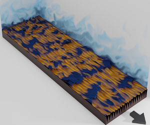
Figure 2. Schematic representation of the simulation domain for the blade riblets (a), where  $L_x$ and $L_y$ are the streamwise and spanwise domain sizes, $A_t$ is the total plan area (purple), $A_c$ is the fluid cross-sectional area (green), $\delta F_u$ is the differential viscous drag, $\delta Q_w$ is the differential wall heat flux and $\delta A_w$ is the differential wetted area. The domain mean height $h \equiv A_c/L_y$ spans from the top boundary to the riblet mean height $z_m$. (b–e) Cross-sectional grid for a sample of each of the four riblet geometries (table 2), where the coordinates are presented in viscous wall units. (b) Triangular T950, (c) trapezoidal TA50, (d) blade BL49 and (e) asymmetric AT50 riblets.
We consider four families of riblet shapes: triangular (figure 2b); trapezoidal (figure 2c); blade (figure 2d); and asymmetric (figure 2e) riblets. We report the simulation parameters for all the cases in table 2. The fluid dynamics of these cases is studied by Endrikat et al. (Reference Endrikat, Modesti, García-Mayoral, Hutchins and Chung2021a,Reference Endrikat, Modesti, MacDonald, García-Mayoral, Hutchins and Chungb) and Modesti et al. (Reference Modesti, Endrikat, Hutchins and Chung2021). For triangular riblets we consider three tip angles  $\alpha = {30}^{\circ }, {60}^{\circ }, {90}^{\circ }$, for trapezoidal riblets we consider $\alpha = {30}^{\circ }$ with $k/s = 0.5$ and for asymmetric riblets we consider $\alpha = {63.4}^{\circ }$ ( $k/s = 0.5$). For the blade riblets, the riblet spacing to the thickness ratio is fixed at $s/t = 5.0$ with $k/s=0.5$. The name of each case consists of one or two letters followed by a number. The letters indicate the riblet geometry: triangular (T); trapezoidal (TA); asymmetric (AT); and blade (BL). The number consists of two digits for all cases, except the triangular riblets (three digits). The two-digit numbers indicate the riblet spacing in wall units $s^+$ (e.g. TA63 has $s^+ = 63$). The three-digit numbers for the triangular riblets indicate $\alpha$ (the first digit is $\alpha /10$) and $s^+$ (the two remaining digits). For example, T321 has $\alpha = {30}^{\circ }$ and $s^+ = 21$. For T950 (triangular riblet with $\alpha = {90}^{\circ }$ and $s^+ = 50$), we include four additional cases from Endrikat et al. (Reference Endrikat, Modesti, MacDonald, García-Mayoral, Hutchins and Chung2021b) to validate the domain size and the grid. Here T950W ( $L^+_y = 450$) and T950N ( $L^+_y = 150$) have wider and narrower spanwise domain sizes, respectively, compared with T950 ( $L^+_y = 250$). Here T950NC ( $\varDelta ^+_x = 8.0, 0.46 \le \varDelta ^+_y \le 8.1$) and T950NVC ( $\varDelta ^+_x = 11.9, 0.65 \le \varDelta ^+_y \le 8.9$) have one level and two levels coarser grid sizes, respectively, compared with T950N ( $\varDelta ^+_x = 6.0, 0.3 \le \varDelta ^+_y \le 7.1$). All the cases are at $Re_\tau = 395$, except T333 where $Re_\tau = 1000$ (triangular riblet with $\alpha = {30}^{\circ }$ and $s^+ = 33$). We also perform two reference smooth-wall simulations at $Re_\tau = 395$ (S395) and $Re_\tau = 1000$ (S1000) to compute the ratios $C_h/C_{h_s}$ and $C_f/C_{f_s}$. The naming of these cases is consistent with Endrikat et al. (Reference Endrikat, Modesti, García-Mayoral, Hutchins and Chung2021a,Reference Endrikat, Modesti, MacDonald, García-Mayoral, Hutchins and Chungb) and Modesti et al. (Reference Modesti, Endrikat, Hutchins and Chung2021). Our choice of $Re_\tau$ ensures that the near-wall flow is fully turbulent. MacDonald et al. (Reference MacDonald, Hutchins and Chung2019) study the Reynolds number effect in turbulent forced convection over rough surfaces (their § 3.2). They compare $Re_\tau = 395$ with $Re_\tau = 590$ in terms of the roughness function $\Delta U^+$ and the temperature difference $\Delta \varTheta ^+$. The difference in $\Delta U^+$ and $\Delta \varTheta ^+$ between the two Reynolds numbers is $0.08$ and $0.1$, respectively.
We perform DNS in a so-called minimal open-channel configuration. In this approach, the domain size  $L_x \times L_y$ is made smaller than the standard full-domain size for channel flow ( $2 {\rm \pi}h \times {\rm \pi}h$, Lozano-Durán & Jiménez (Reference Lozano-Durán and Jiménez2014)). As a result, the computational cost will be reduced (Chung et al. Reference Chung, Chan, MacDonald, Hutchins and Ooi2015). This technique was initially proposed to study the near-wall turbulence in smooth-wall channel flow (Jiménez & Moin Reference Jiménez and Moin1991; Flores & Jiménez Reference Flores and Jiménez2010; Hwang Reference Hwang2013). Later, Chung et al. (Reference Chung, Chan, MacDonald, Hutchins and Ooi2015) and MacDonald et al. (Reference MacDonald, Chung, Hutchins, Chan, Ooi and García-Mayoral2017) adopted this technique to study rough-wall channel flow, demonstrating its accuracy to compute the roughness function $\Delta U^+$. MacDonald et al. (Reference MacDonald, Hutchins and Chung2019) extended the minimal-channel application to turbulent forced convection over rough surfaces, and accurately computed the temperature difference $\Delta \varTheta ^+$.
We show the computational grid for each geometry in figure 2(b–e). The grid points are clustered at the riblet tips and stretched with a hyperbolic-tangent distribution towards the top boundary. For the asymmetric riblets (figure 2e), we perform mesh refinement in the spanwise and wall-normal directions using the adaptive mesh refinement tool Adapt (Cascade Technologies Inc.). In this tool, we specify a set of maximum spacings  $\varDelta ^+_{y_m}, \varDelta ^+_{z_m}$ for a set of heights. The tool creates different mesh zones based on the selected heights and iteratively subdivides the computational cells to meet the target spacings. Specifically, we set $\varDelta ^+_{y_m} = \{ 1.5, 3, 4, 5 \}$ and $\varDelta ^+_{z_m} = \{ 0.9, 2, 4, 6 \}$ for the selected heights of $z^+ - z^+_t \lesssim \{16, 40, 80 \}$ and above, respectively ( $z_t$ is the $z$-coordinate of the riblet tip). We report the grid resolutions in table 2. For the production cases, the number of grid points per riblet spacing ( $n_s \ge 27$) is similar to the previous DNS studies on riblets ( $n_s \ge 24$ in Goldstein, Handler & Sirovich (Reference Goldstein, Handler and Sirovich1995), Goldstein & Tuan (Reference Goldstein and Tuan1998) and García-Mayoral & Jiménez (Reference García-Mayoral and Jiménez2011b)). Also, the grid spacing in the streamwise and spanwise directions ( $\varDelta ^+_x \le 6.5, \varDelta ^+_y \le 7.1$) is similar to the previous DNS studies on riblets ( $\varDelta ^+_x \le 9, \varDelta ^+_y \le 4$ in García-Mayoral & Jiménez (Reference García-Mayoral and Jiménez2011b) and García-Mayoral & Jiménez (Reference García-Mayoral and Jiménez2012)) and roughness ( $\varDelta ^+_x \le 6, \varDelta ^+_y \le 6$ in MacDonald et al. (Reference MacDonald, Hutchins and Chung2019) and Chan et al. (Reference Chan, MacDonald, Chung, Hutchins and Ooi2015)). Nevertheless, a grid-convergence study for the triangular riblet with $\alpha ={90}^{\circ }$ and $s^+ = 50$ (T950) was performed by running one level finer and two levels coarser grids (figure 2 in Endrikat et al. (Reference Endrikat, Modesti, MacDonald, García-Mayoral, Hutchins and Chung2021b)). The reported grid for T950 in table 2 with $n_s = 33, \varDelta ^+_x = 6.0$ and $\varDelta ^+_y \le 7.1$ reaches grid convergence in the mean velocity, turbulent stresses and energy spectra. The same grid yields grid convergence in $C_f/C_{f_s}, C_h/C_{h_s}$ and heat transfer efficiency $\eta \equiv (C_h/C_{h_s})/(C_f/C_{f_s})$. We conclude this by comparing T950N (same grid resolution as T950) with T950NC (one level coarser grid resolution than T950) and T950NVC (two levels coarser grid resolution than T950). The difference between T950N and T950NC in terms of $C_f/C_{f_s}, C_h/C_{h_s}$ and $\eta$ is $0.2\,\%, 0.1\,\%$ and $0.1\,\%$, respectively. Other cases reported in table 2 have similar or finer resolution than T950.
Over riblets, wide Kelvin–Helmholtz (KH) rollers emerge (García-Mayoral & Jiménez Reference García-Mayoral and Jiménez2012). Endrikat et al. (Reference Endrikat, Modesti, MacDonald, García-Mayoral, Hutchins and Chung2021b) demonstrated the suitability of minimal channels for riblets, in particular for the present cases in table 2. They performed domain-independence studies for cases T950 and T321, the former without KH rollers and the latter with the rollers. Endrikat et al. (Reference Endrikat, Modesti, MacDonald, García-Mayoral, Hutchins and Chung2021b) also compared the blade riblet cases BL20 and BL33, computed using minimal channel, with closely matched blade riblet cases 13L and 20L by García-Mayoral & Jiménez (Reference García-Mayoral and Jiménez2012), computed using full-domain simulations. Consistent with the previous minimal channel studies (Chung et al. Reference Chung, Chan, MacDonald, Hutchins and Ooi2015; MacDonald et al. Reference MacDonald, Chung, Hutchins, Chan, Ooi and García-Mayoral2017), with  $L^+_y = 250$ and $L^+_x = 1027$ at $Re_\tau \simeq 395$ and $k^+ \lesssim 40$, the mean velocity is accurately predicted up to $z^+_c \simeq 0.4 L^+_y = 100$ (figure 4 in Endrikat et al. (Reference Endrikat, Modesti, MacDonald, García-Mayoral, Hutchins and Chung2021b)). Also, with this domain size, turbulence remains unaffected (by the domain size) up to $30$ wall units above the riblet crest (§ 3.2 in Endrikat et al. (Reference Endrikat, Modesti, MacDonald, García-Mayoral, Hutchins and Chung2021b)). Therefore, we choose $L^+_y \simeq 250$ and $L^+_x \gtrsim 1027$ at $Re_\tau = 395$, and $L^+_y \simeq 600$ and $L^+_x = 2000$ at $Re_\tau = 1000$. With these choices, we resolve the flow field up to $z^+_c \simeq 100$ ( $Re_\tau = 395$) and $z^+_c \simeq 240$ ( $Re_\tau = 1000$). In § 2.3, we perform domain size study for the velocity and temperature by considering the grid converged case T950 with different domain sizes: T950 ( $L^+_y = 250$) and T950W ( $L^+_y = 450$).
The simulations were run for sufficient flow-through times to obtain statistical uncertainties in  $\Delta U^+$ and $\Delta \varTheta ^+$ of $\pm 0.1$ or less (table 1 in Endrikat et al. (Reference Endrikat, Modesti, MacDonald, García-Mayoral, Hutchins and Chung2021b)). For minimal channels, the required averaging time to obtain a desired level of statistical uncertainty is derived by MacDonald et al. (Reference MacDonald, Chung, Hutchins, Chan, Ooi and García-Mayoral2017) (see § 4). We further checked statistical convergence following Vinuesa et al. (Reference Vinuesa, Prus, Schlatter and Nagib2016) to ensure that the plane and time averaged total stress above the riblet tips is close to linear (§ 2.4 in Endrikat et al. (Reference Endrikat, Modesti, MacDonald, García-Mayoral, Hutchins and Chung2021b)).
2.2. Virtual origin
We need the virtual origin  $d$ to compute $\Delta U^+$ ( $U^+_s - U^+_r$, where subscripts $r$ and $s$ refer to the riblet and smooth cases, respectively) and the temperature difference $\Delta \varTheta ^+$ ( $\varTheta ^+_s - \varTheta ^+_r$). We use $\Delta U^+$ and $\Delta \varTheta ^+$ to compute $C_f$ and $C_h$ (see § 2.3 in MacDonald et al. (Reference MacDonald, Hutchins and Chung2019)). To find $d$, we follow the suggestion by Luchini (Reference Luchini1996). According to Luchini et al. (Reference Luchini, Manzo and Pozzi1991), for a drag reducing riblet ( $\Delta U^+ < 0$) the origin of turbulence is shifted upwards relative to the origin of the riblet mean height $z_m$. This shift appears as a shift in the turbulent part of the Reynolds shear stress $\overline {uw}_T$. Following Endrikat et al. (Reference Endrikat, Modesti, García-Mayoral, Hutchins and Chung2021a), we compute $\overline {uw}_T$ by excluding the form-induced component from the total Reynolds shear stress. Figure 3(a) shows $\overline {uw}_T$ for asymmetric riblets AT15 (black solid line) and AT40 (dashed–dotted line) compared with the smooth wall ( $\circ$).

Figure 3. Profiles of (a,d) turbulent part of Reynolds shear stress  $\overline {uw}_T$, (b,e) turbulent scalar flux $\overline {\theta w}_T$ and (c, f) roughness function $\Delta U^+$ ( $U^+_s - U^+_r$, where subscripts $r$ and $s$ refer to the riblet and smooth cases, respectively) and the temperature difference $\Delta \varTheta ^+$ ( $\varTheta ^+_s - \varTheta ^+_r$). The profiles with black colour correspond to the momentum transport ( $\overline {uw}^+, \Delta U^+$) and those with magenta colour correspond to the temperature transport ( $\overline {\theta w}^+, \Delta \varTheta ^+$). We consider asymmetric riblets AT15 (magenta solid line, black solid line) and AT40 (magenta dashed–dotted line, black dashed–dotted line), and smooth wall case at $Re_\tau = 395$ ( $\circ$). All the quantities in wall units are scaled by $u_\tau$ and $\nu$. Panels (a–c) show the profiles by having the mean riblet height $z_m$ as the origin, and (d–f) show the same profiles by having the virtual origin $d$ as the origin. In (d), $d$ is obtained for the mean velocity by shifting $\overline {uw}_T$, and in (e), $d$ is obtained for the mean temperature by shifting $\overline {\theta w}_T$ (see the text for discussion). In ( f), the profiles of $\Delta U^+$ and $\Delta \varTheta ^+$ are shifted by the values of $d$ obtained from (d) and (e), respectively.
Following Luchini (Reference Luchini1996), we find  $d$ by shifting the $\overline {uw}_T$ profile of the riblet cases to collapse, when plotted against $z-d$, onto the $\overline {uw}_T$ profile of a smooth case at matched $Re_\tau$, when plotted against $z$. We collapse the two profiles at their maximum slope near the wall. This works well for drag-reducing riblets. Endrikat et al. (Reference Endrikat, Modesti, García-Mayoral, Hutchins and Chung2021a) propose an extrapolation for determining $d$ for the other cases of table 2: for each riblet shape at constant $\alpha$ or $t/s$, they find $d$ for the minimum size, e.g. AT15 for asymmetric riblet, and then set the virtual origin of other cases by assuming that $d/k$ is constant. We follow the same approach for the temperature (passive-scalar) field. In figure 3, we consider $\overline {uw}_T$, $\overline {\theta w}_T$, $\Delta U^+$ and $\Delta \varTheta ^+$ for the asymmetric riblet cases AT15 (solid line) and AT42 (dashed–dotted line). In figure 3(a–c), we plot the profiles by taking the riblet mean height $z_m$ as the origin. In figure 3(d–f), we plot the profiles by taking $d$ as the origin. Figure 3( f) shows that accounting for the origin $d$ at the present $Re_\tau$ where the log layer is nascent, results in a wider plateau of near constant $\Delta U^+$ and $\Delta \varTheta ^+$, thereby allowing a more robust measure of the roughness function and temperature difference, and hence $C_f$ and $C_h$. In figure 3( f), the values of $d$ for plotting $\Delta U^+$ and $\Delta \varTheta ^+$ are obtained, respectively, from $\overline {uw}_T$ (figure 3d) and $\overline {\theta w}_T$ (figure 3e). By analysing several riblet cases, we find that the values of $d$ obtained from $\overline {uw}_T$ (for $\Delta U^+$) and $\overline {\theta w}_T$ (for $\Delta \varTheta ^+$) are very close to each other (within 3 % of $k$). Therefore, in the rest of this paper we use one value of $d$ (from $\overline {uw}_T$) to compute $\Delta U^+$ and $\Delta \varTheta ^+$.
2.3. Skin-friction coefficient and Stanton number
The skin-friction coefficient  $C_f$ and Stanton number $C_h$ are defined as
 \begin{equation} C_f \equiv \frac{2\left\langle \tau_w \right\rangle}{\rho U^2_b}=\frac{2}{{U^+_b}^2}, \quad C_h \equiv \frac{\left\langle q_w \right\rangle}{\rho c_p U_b \varTheta_m} = \frac{1}{U^+_b \varTheta^+_m}, \end{equation}
where  $U^+_b$ is the bulk velocity and $\varTheta ^+_m$ is the mixed-mean temperature (Owen & Thomson Reference Owen and Thomson1963; Bird, Stewart & Lightfoot Reference Bird, Stewart and Lightfoot1962). Here
 \begin{align} U^+_b \equiv \frac{1}{\left( z^+_{max}-z^+_{min} \right)} \int_{z^+_{min}}^{z^+_{max}} U^+ \,{\rm d}z^+, \quad \varTheta^+_m \equiv \frac{1}{U^+_b\left( z^+_{max}-z^+_{min} \right)} \int_{z^+_{min}}^{z^+_{max}} U^+ \varTheta^+ \,{\rm d}z^+ \end{align}
where  $z^+_{min}$ and $z^+_{max}$ are the bottom of the riblet groove and top boundary of the domain, respectively. The mixed mean temperature is the temperature one would obtain if the fluid from the channel was discharged into a container and was thoroughly mixed. According to (2.5a,b), we need $U^+_b$ and $\varTheta ^+_m$ to compute $C_f$ and $C_h$. However, we cannot compute $U^+_b$ and $\varTheta ^+_m$ by directly integrating $U^+$ and $\varTheta ^+$ profiles from the minimal-channel configuration. We show this in figure 4. We compare the $U^+$ profile (figure 4a) and $\varTheta ^+$ profile (figure 4b) between the smooth wall case S395 in minimal domain (blue solid line, blue dotted line, $L^+_x \times L^+_y = 1027 \times 250$) and the smooth wall DNS of Kawamura et al. (Reference Kawamura, Ohsaka, Abe and Yamamoto1998) in full domain ( $\circ$, black, $L^+_x \times L^+_y = 2528 \times 1264$). The minimal-domain $U^+$ and $\varTheta ^+$ profiles (blue solid line) reproduce the full-domain profiles ( $\circ$, black) up to $z^+_c \simeq 0.4 L^+_y \simeq 100$. Beyond $z^+_c$, the minimal-domain profiles (blue dotted line) depart from the full-domain profiles ( $\circ$, black), but the universal outer layers can easily be reconstructed. Importantly, the minimal domain resolves the flow up to $z^+_c$ (Chung et al. Reference Chung, Chan, MacDonald, Hutchins and Ooi2015; MacDonald et al. Reference MacDonald, Chung, Hutchins, Chan, Ooi and García-Mayoral2017, Reference MacDonald, Hutchins and Chung2019), which includes the effects of different riblet shapes and sizes. Beyond $z^+_c$, we reconstruct the full-domain profiles (blue dashed line in figure 4a,b) using the composite profiles of full-domain channel flow ( $U^+_f, \varTheta ^+_f$):
 $$\begin{gather} U^+_f = \frac{1}{\kappa_u}\ln(z^+-d^+) + B_u + \frac{2\varPi_u}{\kappa_u}\mathcal{W}_u(z/h) - \Delta U^+, \quad z^+ \ge z^+_c, \end{gather}$$
 $$\begin{gather}\varTheta^+_f = \frac{1}{\kappa_\theta}\ln(z^+-d^+) + B_\theta + \frac{2\varPi_\theta}{\kappa_\theta}\mathcal{W}_\theta(z/h) - \Delta \varTheta^+, \quad z^+ \ge z^+_c . \end{gather}$$
We first reconstruct our smooth cases S395 and S1000 ( $\Delta U^+ = \Delta \varTheta ^+ = 0$). To verify our reconstruction, we use the DNS data of full-domain channel flow at $Re_\tau = 395, Pr=0.71$ (Kawamura et al. Reference Kawamura, Ohsaka, Abe and Yamamoto1998) and $Re_\tau = 1020, Pr=0.71$ (Abe, Kawamura & Matsuo Reference Abe, Kawamura and Matsuo2004). We choose $\kappa _u = 0.4$ and $\kappa _\theta = 0.46$ following Pirozzoli, Bernardini & Orlandi (Reference Pirozzoli, Bernardini and Orlandi2016). We set the offsets $B_u = 5.2$ and $B_\theta = 3.8$ (for $Pr = 0.7$), to make the profiles continuous at $z^+_c$. For the wake functions $\mathcal {W}_u$ and $\mathcal {W}_\theta$, we use the formulation for channel flow by Nagib & Chauhan (Reference Nagib and Chauhan2008) (see their equation (12)). We set the velocity wake parameter $\varPi _u = 0.05$, as suggested by Nagib & Chauhan (Reference Nagib and Chauhan2008) (see their figure 6). We set the temperature wake parameter $\varPi _\theta = 0.08$, to obtain the best fit with the reference DNS (figure 4b, the inset). After reconstructing the smooth channel profiles, we shift them by $\Delta U^+$ and $\Delta \varTheta ^+$ (table 2) to reconstruct the region above $z^+_c$ for the riblet cases.

Figure 4. Assessing the accuracy of the minimal-domain approach for (a,b) smooth case S395 and (c,d) triangular riblet case with  $\alpha = {90}^{\circ }$ and $s^+ = 50$. Panels (a,b), respectively, compare $U^+$ and $\varTheta ^+$ profiles between S395 (blue solid line, blue dotted line) and DNS of full-domain smooth channel flow ( $\circ$, black, Kawamura et al. (Reference Kawamura, Ohsaka, Abe and Yamamoto1998)) at matched $Re_\tau = 395$ and $Pr = 0.71$. The minimal-domain profiles (blue solid line) reproduce the full-domain profiles ( $\circ$, black) up to $z^+_c \simeq 0.4 L^+_y \simeq 100$. Beyond $z^+_c$, the minimal-domain profiles (blue dotted line) depart from the full-domain profiles ( $\circ$, black), because the minimal domain correctly resolves the flow only up to $z^+_c$ (Chung et al. Reference Chung, Chan, MacDonald, Hutchins and Ooi2015; MacDonald et al. Reference MacDonald, Chung, Hutchins, Chan, Ooi and García-Mayoral2017, Reference MacDonald, Hutchins and Chung2019). Beyond $z^+_c$, the profiles are reconstructed (blue dashed line) using the composite profiles of Nagib & Chauhan (Reference Nagib and Chauhan2008). Panels (c,d), respectively, compare $U^+$ and $\varTheta ^+$ profiles between two domain sizes of the same riblet case (triangular riblet with $\alpha = {90}^{\circ }$ and $s^+ = 50$); T950 with $L^+_y = 250$ (black solid line, black dotted line) and T950W with $L^+_y = 450$ (red solid line, red dotted line). Beyond $z^+_c$, the minimal-domain profiles (black dotted line, red dotted line) are replaced by the composite profiles (black dashed line, red dashed line) based on Nagib & Chauhan (Reference Nagib and Chauhan2008).
We show the accuracy of minimal-domain simulation and profile reconstruction in figure 4(a,b) by comparing the resolved and reconstructed profiles for S395 (blue solid line, blue dashed line) with the full-domain reference data ( $\circ$, black) at $Re_\tau = 395$ and $Pr = 0.71$. Figure 4(a) compares the $U^+$ profiles and figure 4(b) compares the $\varTheta ^+$ profiles. We calculate $C_f$ and $C_h$ (2.5a,b) by integrating the resolved (blue solid line) and reconstructed (blue dashed line) portions of the profiles. The obtained $C_{f_s}$ and $C_{h_s}$ for S395 (blue solid line, blue dashed line) are different by $0.4\,\%$ and $0.2\,\%$, respectively, compared with the $C_{f_s}$ and $C_{h_s}$ from the reference full-domain DNS ( $\circ$, black). We further show the accuracy of minimal-domain simulation for the triangular riblet with $\alpha = {90}^{\circ }$ and $s^+ = 50$ (figure 4c,d). We compare different domain sizes: T950 with $L^+_y = 250$ (black solid line, black dotted line) and T950W with $L^+_y = 450$ (red solid line, red dotted line). We compare the $U^+$ profiles (figure 4c) and $\varTheta ^+$ profiles (figure 4d). We reconstruct the profiles beyond $z^+_c \simeq 0.4L^+_y \simeq 100$ for T950 (black dashed line) and beyond $z^+_c \simeq 0.4L^+_y \simeq 180$ for T950W (red dashed line). The profiles from the two domain sizes agree well with each other, both in the resolved (solid lines) and reconstructed (dashed lines) parts. The difference in $C_f/C_{f_s}, C_h/C_{h_s}$ and $\eta$ between the two domain sizes is $1\,\%, 0.5\,\%$ and $0.4\,\%$, respectively. The reported uncertainties for $C_f/C_{f_s}, C_h/C_{h_s}$ and $\eta$ take into account the uncertainty due to the domain size and profile reconstruction together. These quantities are obtained by integrating the resolved portion of the profiles (from the minimal-domain simulation) and the reconstructed portion.
As mentioned in § 1, different studies use different Reynolds number definitions for matching the flow condition between the riblet and smooth surfaces. Experimental studies (Walsh & Weinstein Reference Walsh and Weinstein1979; Choi & Orchard Reference Choi and Orchard1997) consider the developing turbulent boundary layer, and use Reynolds number  $Re_x \equiv U_\infty x/\nu$ based on the free stream velocity $U_\infty$ and the distance $x$ downstream of the test section entrance. Numerical studies (Stalio & Nobile Reference Stalio and Nobile2003; Jin & Herwig Reference Jin and Herwig2014) consider channel flow, and use bulk Reynolds number $Re_b \equiv U_b h/\nu$. Here, we also calculate $C_f/C_{f_s}$ and $C_h/C_{h_s}$ at a matched $Re_b$. For the cases simulated at $Re_\tau = 395$ (table 2), we match at $Re_b = 7038$. For the case T333 simulated at $Re_\tau = 1000$ (triangular riblet at $\alpha = {30}^{\circ }, s^+ \simeq 33$), we match at $Re_b = 20192$. These matched values of $Re_b$ correspond to $Re_\tau = 395$ (at $Re_b = 7038$) and $Re_\tau = 1000$ (at $Re_b = 20192$) for smooth-wall channel flow.
3. Results
3.1. Global investigation of Reynolds analogy
Figure 5 is a comprehensive plot measuring Reynolds analogy for all the cases in table 2. Each marker in figure 5(a–e) corresponds to one riblet case. To identify the markers, we draw a chart above figure 5(a–e) that contains the geometry of each riblet case and its marker. In the chart, we arrange the riblets horizontally based on their spacings  $s^+$ and we arrange the riblets vertically based on their shapes. To facilitate inspection, we show the performance relative to Reynolds analogy of all cases in three plots: triangular riblets (figure 5a); trapezoidal riblets (figure 5b); blade and asymmetric riblets (figure 5c). We also include some comparable cases of the previous studies: Walsh & Weinstein (Reference Walsh and Weinstein1979) (green bullets), Choi & Orchard (Reference Choi and Orchard1997) (red bullet) and Jin & Herwig (Reference Jin and Herwig2014) (blue filled triangle). We draw an ellipse around each comparable pair, both in the chart and in the Reynolds analogy plots.

Figure 5. Reynolds analogy plot for all the cases (table 2) and comparable cases from previous studies. The top chart shows their geometries. In the chart, from top to bottom, riblet geometries are arranged as the following: triangular riblets with  $\alpha = {30}^{\circ }, {60}^{\circ }, {90}^{\circ }$; trapezoidal riblets; blade riblets; and asymmetric riblets. In the horizontal direction, riblets are arranged based on their spacing $s^+$. The previous cases are shown with filled symbols. For each comparable pair from the previous studies and the present data, we draw an underline in the top chart, and we draw an ellipse in the Reynolds analogy plots. We compare different riblet geometries in separate plots: (a) triangular riblets (T3, T6, T9); (b) trapezoidal riblets (TA); (c) blade BL and asymmetric AT riblets. Panels (d,e) magnify the Reynolds analogy plot within the dotted rectangles shown in (a), and only show Reynolds analogy for the triangular riblet at (d) $\alpha = {30}^{\circ }$ and $s^+ = 21$, and (e) $\alpha = {30}^{\circ }$ and $s^+ = 33$. In the chart, the highlighted cases in bold (T333, T950, TA63, BL49) are further analysed in § 3.2.
The trapezoidal (figure 5b), blade and asymmetric riblets (figure 5c) break the Reynolds analogy in an unfavourable way; especially, as  $s^+$ increases. We quantify this in table 2 (the rightmost column) by reporting the heat transfer efficiency $\eta \equiv (C_h/C_{h_s})/(C_f/C_{f_s})$. For the trapezoidal, blade and asymmetric riblets with $s^+ > 50$, $\eta$ varies between $0.955$ and $0.975$. For these cases, if we take into account all the possible simulation uncertainties, $\eta$ is still below unity. We consider the uncertainties due to the statistical averaging and grid (§ 2.1), as well as the domain size and profile reconstruction (§ 2.3). To estimate how the statistical uncertainty of $\pm 0.1$ in $\Delta U^+$ and $\Delta \varTheta ^+$ (§ 2.1) propagate to $\eta$, we use Taylor series expansion of the analytical relation for $\eta (\Delta U^+, \Delta \varTheta ^+)$ (see (11) in Aupoix (Reference Aupoix2015)). For the case BL49, we obtain statistical uncertainty of $\pm 0.008$ in $\eta$ with $\Delta U^+ = 1.84 \pm 0.1, \Delta \varTheta ^+ = 1.10 \pm 0.1$ and the smooth wall coefficients $C_{f_s} = 0.0063, C_{h_s} = 0.0037$ at $Re_\tau = 395$. We also report an uncertainty of $\pm 0.001$ in $\eta$ due to the grid, and a total uncertainty of $\pm 0.004$ due to the domain size and profile reconstruction (§§ 2.1 and 2.3). Summing all the possible uncertainties for BL49, we report $\eta = 0.974 \pm 0.013$, hence we find a statistically robust unfavourable breaking of the global Reynolds analogy. However, the triangular riblets (figure 5a) break the Reynolds analogy to a lesser extent. A closer inspection of figure 5(a) (as shown in figure 5d,e) reveals that the triangular riblet cases T321 with $\alpha = {30}^{\circ }, s^+ = 21$ (figure 5d) and T333 with $\alpha = {30}^{\circ }, s^+ = 33$ (figure 5e) fall onto or slightly above the Reynolds analogy line. Among all the riblet cases in table 2, only T321 and T333 yield $\eta >1$ ( $1.007$ and $1.012$, respectively). These values of $\eta$ are marginally higher than unity. With the levels of simulation uncertainties in $\eta$, it is not possible to definitely conclude that T321 and T333 break the global Reynolds analogy favourably. For the case T321, we obtain statistical uncertainty of $\pm 0.008$ in $\eta$ with $\Delta U^+ = 0.83 \pm 0.1, \Delta \varTheta ^+ = 0.87 \pm 0.1$ and the smooth wall coefficients $C_{f_s} = 0.0063, C_{h_s} = 0.0037$ at $Re_\tau = 395$. For the case T333, we obtain statistical uncertainty of $\pm 0.008$ in $\eta$ with $\Delta U^+ = 2.75 \pm 0.1, \Delta \varTheta ^+ = 2.35 \pm 0.1$ and the smooth wall coefficients $C_{f_s} = 0.0049, C_{h_s} = 0.0029$ at $Re_\tau = 1000$. By adding the grid size, domain size and profile reconstruction uncertainties in $\eta$ ( $\pm 0.005$), we report $\eta = 1.007 \pm 0.013$ and $\eta = 1.012 \pm 0.013$ for T321 and T333, respectively. Hence the observed favourable breaking is within the uncertainty bounds. However, we can definitively conclude that as the viscous-scaled riblet spacing increases from $s^+ = 21$ (T321, figure 5d) to $s^+ = 33$ (T333, figure 5e), the triangular riblet with $\alpha = {30}^{\circ }$ preserves its performance close to the Reynolds analogy line. In contrast, the other riblet shapes (e.g. figure 5b,c) depart from the Reynolds analogy line towards the unfavourable side as $s^+$ increases; this trend is similar to conventional rough surfaces (figure 1a), although roughness departs farther from the Reynolds analogy line. These observations motivate us to investigate the flow physics of T333 ( $\eta \simeq 1.012$) compared with the other riblet cases ( $\eta < 1$) in § 3.2.
Walsh & Weinstein (Reference Walsh and Weinstein1979) experimentally investigated triangular riblets with  $\alpha \simeq {30}^{\circ }$ (green bullets in figure 5a) in addition to sharper and blunter triangular riblets with $\alpha \simeq {16}^{\circ }$ and ${40}^{\circ }$, respectively. To reconstruct the Reynolds analogy plot of Walsh & Weinstein (Reference Walsh and Weinstein1979), we use their reported $C_f/C_{f_s}$ and $\eta$ (see their figures 2 and 3). Walsh & Weinstein (Reference Walsh and Weinstein1979) observe different behaviour in the heat transfer efficiency of triangular riblets with $\alpha \lesssim {30}^{\circ }$ (having $\eta > 1$) compared with those with $\alpha \simeq {40}^{\circ }$ (having $\eta < 1$). Consistently, we see different behaviour in the heat transfer efficiency of triangular riblets with $\alpha = {30}^{\circ }$ ( $\times, *$ with $\eta \gtrsim 1$) and those with $\alpha = {60}^{\circ }$ ( $\bigtriangleup$, $\diamond$ with $\eta < 1$). However, for triangular riblets with $\alpha = {30}^{\circ }$, Walsh & Weinstein (Reference Walsh and Weinstein1979) report a more noticeable favourable breaking of the global Reynolds analogy (green bullets in figure 5a) compared with our observation in the current study ( $\times, *$ in figure 5d,e). The different observations between the experimental and DNS data could be due to the factors discussed in § 1 (flow configuration, definition of $C_f, C_h$ and Reynolds number) in addition to experimental uncertainties. Nevertheless, the consistent observation of the unique behaviour of triangular riblets with $\alpha = {30}^{\circ }$ calls for further exploration of the underlying flow physics. Walsh & Weinstein (Reference Walsh and Weinstein1979) could not investigate the underlying flow physics, owing to experimental limitations. An advantage of DNS is the high-fidelity dataset, particularly in the riblet grooves, to probe the underlying flow structure. We perform such investigations in the following sections.
3.2. Local investigation of Reynolds analogy
The Reynolds analogy plots (figure 5) are constructed based on  $C_f \equiv 2\left \langle \tau _w \right \rangle /(\rho U^2_b)$ and $C_h \equiv \left \langle q_w \right \rangle /(\rho c_p U_b \varTheta _m)$. These quantities are obtained by integrating $\tau _w$ and $q_w$ over time and the entire riblet surface. Therefore, breaking of the analogy between $C_f/C_{f_s}$ and $C_h/C_{h_s}$ (based on $\left \langle \tau _w \right \rangle$ and $\left \langle q_w \right \rangle$) is due to the breaking of the analogy between their local instantaneous counterparts (based on $\tau _w$ and $q_w$). We denote the local counterparts as $\hat {C}_f/C_{f_s}$ and $\hat {C}_h/C_{h_s}$. We use the prefix ‘global’ when we mention $C_f/C_{f_s}$ and $C_h/C_{h_s}$, and we use the prefix ‘local’ when we mention $\hat {C}_f/C_{f_s}$ and $\hat {C}_h/C_{h_s}$. In § 3.2.1, we study the breaking of the analogy between the local $\hat {C}_f/C_{f_s}$ and $\hat {C}_h/C_{h_s}$, hence local breaking of Reynolds analogy. Then in §§ 3.2.2, 3.2.3 and 3.2.4 we uncover the important flow mechanisms that are associated with the local breaking of Reynolds analogy. We identify the favourable and unfavourable flow mechanisms depending on how they locally break Reynolds analogy. Finally, in §§ 3.2.3 and 3.2.4 we analyse the contribution of each important flow mechanism to the global breaking of Reynolds analogy. We investigate how this contribution depends on the riblet geometry.
3.2.1. Local skin-friction coefficient versus local Stanton number
We define the local  $\hat {C}_f$ and $\hat {C}_h$ (figure 6) so that they are relatable to their global counterparts (figure 5). In figure 6, we demonstrate how we define $\hat {C}_h$ for the blade riblet BL49, as an example. We follow the same procedure for $\hat {C}_f$.

Figure 6. Different definitions of local Stanton number for blade riblet BL49, in different coordinates such that  $C_h = (1/A_w)\int _{A_w} \hat {C}_h dA_w$. (a) Here $C^*_h = q_w/(\rho c_p U_b \varTheta _m )$ is a temporary definition based on local wall heat flux $q_w = \mathrm {d}Q_w/\mathrm {d}A_w$ in $x$–
$x$– $y$ coordinate; (b) $C^*_h$ the same as (a) in $x$–
$x$– $\xi$ coordinate; (c) $\hat {C}_h = \hat {q}_w/(\rho c_p U_b \varTheta _m)$ in $x$–
$x$– $\xi$ coordinate based on compensated $\hat {q}_w = (A_w/A_t) q_w$, where $A_w$ and $A_t$ are the total wetted area and total planar area (figure 2), respectively. In the schematic on the top right we colour each part of the three-dimensional sketch of blade riblets. Next to (a,c), we draw the sketch in $x$–
$x$– $y$ and $x$–
$x$– $\xi$ coordinates, respectively. This highlights which parts of the blade surface become visible in each coordinate system.
To the global  $C_h$, each part of the riblet surface contributes proportionally to its wetted area. For example, in the schematic in figure 6 (top right), $C_h$ is obtained through integration of the local wall heat flux $q_w = \delta Q_w/\delta A_w$ over time, and also spatially over the vertical sidewalls (in black), base (in grey) and the crest (in green). Therefore, local investigation based on a view of $q_w$ in the $xy$-plane would suffer from distortion (figure 6a), because the vertical sidewalls are missing. Even for other riblets with tilted sidewalls, the $xy$-plane is not suitable. Therefore, we define a new unfolded coordinate $\xi$ with two properties: (1) it is tangent to the riblet surface, and (2) it is normal to the $x$-coordinate. In the $x\xi$-plane (figure 6b), each part of the riblet surface contributes proportionally to its wetted area. Therefore, we study the local Stanton number in the $x\xi$-plane. A possible definition for local Stanton number is $C^*_h \equiv q_w/(\rho c_p U_b \varTheta _m)$ (figure 6b). Averaging $C^*_h$ over the $x\xi$-plane and time yields $Q_w/(\rho c_p U_b \varTheta _m A_w)$, which differs from the global $C_h \equiv Q_w/(\rho c_p U_b \varTheta _m A_p)$ by a factor of $A_w/A_p$. Therefore, we define the local $\hat {C}_h = (A_w/A_p) C^*_h$ (figure 6c) such that its average over the $x\xi$-plane and time yields $(1/T) (1/A_w)\int _T \int _{A_w}\hat {C}_h \delta A_w\, {\rm d}t = C_h$ where $T$ is the averaging time period. We define $\hat {C}_f$ correspondingly.
Figure 7 compares the global Reynolds analogy (figure 7a,c,e,g) with the local Reynolds analogy (figure 7b,d, f,h) for selected riblet cases (highlighted in bold in the top chart of figure 5). For fair comparison of the global Reynolds analogy between different cases, the size of the plotting range is the same for all figure 7(a,c,e,g). The selected cases have different riblet shapes with a diverse global Reynolds analogy behaviour. The case T333 (figure 7g,h, triangular riblet at  $\alpha = {30}^{\circ }, s^+ = 33$) falls above the Reynolds analogy line, TA63 (figure 7c,d, trapezoidal riblet at $s^+ = 63$) and BL49 (figure 7e, f, blade riblet at $s^+ = 49$) fall below the Reynolds analogy line, and T950 (figure 7a,b, triangular riblet at $\alpha = {90}^{\circ }, s^+ = 50$) almost falls onto the Reynolds analogy line. Our findings based on investigation of these cases are sufficient to explain the behaviour of other cases of the present study. The unique behaviour of T333 in its global Reynolds analogy (§ 3.1, figures 5e and 7g) is also seen in its local Reynolds analogy (figure 7h). In this case, there are distinct patches of $\hat {C}_f < 0$ (highlighted with green boundaries). These patches locally break the Reynolds analogy, because negative $\hat {C}_f$ does not have an analogue in $\hat {C}_h$. Solution to (2.3) obeys $\theta \ge 0$, hence $\hat {C}_h \ge 0$. Therefore, the larger and stronger the patches of $\hat {C}_f<0$ are in a riblet case, the stronger is the local breaking of Reynolds analogy. In T333, patches of $\hat {C}_f<0$ occupy a substantial fraction of the wetted area. To quantify this observation, we report the area of $\hat {C}_f<0$ ( $A_{\hat {C}_f<0}$) at the top of figure 7(b,d, f,h). For T333, $A_{\hat {C}_f<0} \simeq 0.28 A_w$ (figure 7h). However, for the unfavourable cases TA63 and BL49, $A_{\hat {C}_f<0} \simeq 0.01 A_w$ and $0.08A_w$, respectively (figure 7d, f). For T950 that preserves Reynolds analogy, $A_{\hat {C}_f<0} \simeq 0.01 A_w$ (figure 7b). Additionally, in T333 patches of $\hat {C}_f<0$ are more negative than their counterparts in the other riblet cases. To support this observation, we conditionally average $\hat {C}_f/C_{f_s}$ over $A_{\hat {C}_f<0}$, i.e. $\bar {C}_f/C_{f_s}\vert _{\hat {C}_f<0} = (1/A_{\hat {C}_f<0})\int _{A_{\hat {C}_f<0}} \hat {C}_f/C_{f_s} \delta A_w$, and report it on top of figure 7(b,d, f,h). For T333, $\bar {C}_f/C_{f_s}\vert _{\hat {C}_f<0} \simeq -0.74$ (figures 7h), whereas for T950, TA63 and BL49, $\bar {C}_f/C_{f_s}\vert _{\hat {C}_f<0} \simeq -0.07, -0.09$ and $-0.22$, respectively (figure 7b,d, f).

Figure 7. Investigation of local  $\hat {C}_f/C_{f_s}$ and local $\hat {C}_h/C_{h_s}$ (b,d, f,h) for selected cases of figure 5. Panels (a,c,e,g) are Reynolds analogy plots for these cases; for fair comparison, the size of the plotting range is $0.05$ for both $C_f/C_{f_s}$ and $C_h/C_{h_s}$, for all cases. (a,b) Triangular riblet T950 at $\alpha = {90}^{\circ },s^+ \simeq 50$; (c,d) trapezoidal riblet TA63 at $s^+ \simeq 63$; (e, f) blade riblet BL49 at $s^+ \simeq 49$; (g,h) triangular riblet T333 at $\alpha = {30}^{\circ },s^+ \simeq 33$; for T333 we only show the range $0 \le x^+, \xi ^+ \le 1000$ for consistent plotting range with other cases. In (b,d, f,h), local $\hat {C}_f/C_{f_s}$ is on the left-hand subpanel and local $\hat {C}_h/C_{h_s}$ is on the right-hand subpanel. Regions of $\hat {C}_f<0$ are bordered with green lines. For each case, we report the fraction of the wetted area $A_w$ where $\hat {C}_f<0$ ( $A_{\hat {C}_f<0}$). We also report the conditionally averaged $\hat {C}_f/C_{f_s}$ over $A_{\hat {C}_f<0}$ given as $\bar {C}_f/C_{f_s}\vert _{\hat {C}_f<0}$.
From the analysis in this section, we conjecture that the unique behaviour of T333 in global Reynolds analogy (figures 5e and 7g) is due to the large proportion of the wetted area occupied by strong patches of  $\hat {C}_f<0$. We investigate the source of negative $\hat {C}_f$ next.
3.2.2. Source of negative skin-friction coefficient: KH rollers
In figure 8, the flow near the riblet grooves is visualised for T950 (figure 8a,b) and T333 (figure 8c,d): in these cases, patches of negative  $\hat {C}_f$ occupy $0.01A_w$ and $0.28A_w$, respectively. To capture coherent structures, we plot the isosurfaces of pressure fluctuations (subtracted from the $xy$-plane and time averaged pressure) $p'^+ \equiv p'/(\rho u^2_\tau ) = -5$, and the wall-normal velocity fluctuations $w'^+ \equiv w'/u_\tau$ at the riblet crest. Figure 8(c,d), corresponding to T333, reveal that patches of negative $\hat {C}_f$ are due to KH rollers. These rollers are elongated in the spanwise direction, as evidenced in the $p'^+$ isosurfaces and $w'^+$ field (figure 8c). The rollers create local flow reversals inside the riblet groove (figure 8d), hence highly negative patches of $\hat {C}_f$ (figure 7h). For T950 (figure 8a,b) no KH roller is visible, hence patches of negative $\hat {C}_f$ are hardly detected (figure 7b).

Figure 8. Visualisation of the flow for (a,b) triangular riblet T950 at  $\alpha = {90}^{\circ },s^+ \simeq 50$, and (c,d) triangular riblet T333 at $\alpha = {30}^{\circ },s^+ \simeq 33$. In (a,c), we plot the instantaneous fields of wall-normal fluctuating velocity $w'^+$ at the riblet crest, overlaid by the isosurfaces of fluctuating pressure (subtracted from the $xy$-plane and time averaged pressure) $p'^+ \equiv p'/(\rho u^2_\tau ) = -5$ (coloured in blue) to identify KH rollers. In (c) for consistency with (a), we only show $1000$ and $300$ wall units of T333 in the $x^+$ and $y^+$ directions. In (b,d), we plot the flow field on an $xz$-plane passing through the middle of the groove (at $y^+ = 125$ and $283$ in panels (b) and (d), respectively). The horizontal long-dashed magenta line locates the riblet crest. The vertical axis for each plane is $(z-z_w)^+$ where $z_w$ is the $z$-coordinate at the bottom of the groove. On the $xz$-plane, we plot the streamwise velocity field $u^+$ overlaid by the $(u^+,w^+)$ streamlines. We also overlay the temperature profiles $\theta ^+$ (green lines) at two $x^+$ locations. Note that the top axis $x^+$ corresponds to the $u^+$ field and the streamlines, and the bottom axis corresponds to the $\theta ^+$ profiles.
Formation of KH rollers was previously reported over blade riblets and triangular riblets with  $\alpha = {30}^{\circ }$ (García-Mayoral & Jiménez Reference García-Mayoral and Jiménez2011b; Endrikat et al. Reference Endrikat, Modesti, García-Mayoral, Hutchins and Chung2021a,Reference Endrikat, Modesti, MacDonald, García-Mayoral, Hutchins and Chungb). Specifically, Endrikat et al. (Reference Endrikat, Modesti, García-Mayoral, Hutchins and Chung2021a,Reference Endrikat, Modesti, MacDonald, García-Mayoral, Hutchins and Chungb) detected these structures over the blade riblets BL20, BL33, BL39, BL49 and triangular riblets T310, T321, T333 (see figure 9 in Endrikat et al. (Reference Endrikat, Modesti, García-Mayoral, Hutchins and Chung2021a)). They observed that KH rollers over the triangular riblets with $\alpha = {30}^{\circ }$ are much stronger than over the blade riblets (see figure 6 in Endrikat et al. (Reference Endrikat, Modesti, García-Mayoral, Hutchins and Chung2021a)). Kelvin–Helmholtz rollers are also reported over environmental canopies such as terrestrial (Raupach, Finnigan & Brunei Reference Raupach, Finnigan and Brunei1996) and aquatic canopies (Ghisalberti & Nepf Reference Ghisalberti and Nepf2002). These rollers exchange scalar and momentum between the canopy and the overlaying flow (Ghisalberti & Nepf Reference Ghisalberti and Nepf2004, Reference Ghisalberti and Nepf2005; Nepf et al. Reference Nepf, Ghisalberti, White and Murphy2007).
Riblets trigger KH rollers because (1) a mixing layer forms between the slow-moving flow inside the groove and the fast-moving flow above the groove, and (2) the crest has wall-normal permeability to develop flow instability (García-Mayoral & Jiménez Reference García-Mayoral and Jiménez2011a,Reference García-Mayoral and Jiménezb, Reference García-Mayoral and Jiménez2012). Endrikat et al. (Reference Endrikat, Modesti, García-Mayoral, Hutchins and Chung2021a) discover that the riblet geometries that trigger KH rollers (1) have a high level of permeability, and (2) cause a high shear in the mixing layer. Endrikat et al. (Reference Endrikat, Modesti, García-Mayoral, Hutchins and Chung2021a) propose two parameters based on these conditions. The viscous-scaled square root of the groove area  $\ell ^+_g$ is correlated with the wall-normal permeability (figure 13b in Endrikat et al. (Reference Endrikat, Modesti, García-Mayoral, Hutchins and Chung2021a)). Also, large drag at the riblet tip causes high-shear mixing layer (figure 15a in Endrikat et al. (Reference Endrikat, Modesti, García-Mayoral, Hutchins and Chung2021a)). The formation of KH rollers occurs when $15 \lesssim \ell ^+_g \lesssim 40$ and the drag at the tip reaches $50\,\%$ to $90\,\%$ of the total wall drag (figure 15c in Endrikat et al. (Reference Endrikat, Modesti, García-Mayoral, Hutchins and Chung2021a)). The case T333 (figure 8c,d) satisfies these conditions.
Kelvin–Helmholtz rollers have a noticeable impact on the thermal field. They create an isothermal layer of  $\theta \approx 0$ inside the riblet valley. In figure 8(b,d), we plot instantaneous profiles of $\theta ^+$ on an $xz$-plane passing through the middle of the riblet groove. For T333 (figure 8d) where KH rollers are strong, profiles of $\theta ^+$ approach zero inside the valley (with the slope $\partial \theta / \partial z \simeq 0$). As a result, patches of $\hat {C}_h \simeq 0$ appear (figure 7h). On the other hand, for T950 (figure 8b) where KH rollers are absent, such a quiescent thermal field does not appear.
We find some resemblance between KH rollers and the mechanism for breaking the Reynolds analogy through wall blowing/suction (Higashi, Mamori & Fukagata Reference Higashi, Mamori and Fukagata2011; Hasegawa & Kasagi Reference Hasegawa and Kasagi2011; Yamamoto et al. Reference Yamamoto, Hasegawa and Kasagi2013; Kaithakkal et al. Reference Kaithakkal, Kametani and Hasegawa2020, Reference Kaithakkal, Kametani and Hasegawa2021). Wall blowing/suction generates a travelling-wave-like control input that is almost uniform in the spanwise direction and periodic in the streamwise direction. Similarly, KH rollers are spanwise-elongated structures that are periodically advected in the streamwise direction. Wall blowing/suction is an active mechanism, hence it demands an additional actuation cost. However, KH rollers are passively generated, hence demand no additional cost.
Our analysis so far shows the importance of KH rollers in local breaking of the Reynolds analogy. The structure of KH rollers consists of alternating reversed and forward flows (see the streamlines in figure 8d). The reversed flow is associated with the local favourable breaking of the Reynolds analogy ( $\hat {C}_f/C_{f_s} < 0 < \hat {C}_h / C_{h_s}$). On the other hand, the forward flow could cause local unfavourable breaking of the Reynolds analogy if $\hat {C}_f/C_{f_s} > \hat {C}_h / C_{h_s} > 0$. There are also other flow mechanisms that interact with the wall. Each mechanism could locally maintain or break the Reynolds analogy, and each of these mechanisms potentially interact or modulate one another. The global Reynolds analogy behaviour results from a complex interplay between all the wall-interacting flow mechanisms. In the next section, we study the wall effect of all the flow mechanisms; we assess the probability of all the wall events in the $(\hat {C}_f/C_{f_s} , \hat {C}_h / C_{h_s})$ space. We present evidence that KH rollers are the primary mechanisms for the local favourable breaking of the Reynolds analogy. This is due to the flow reversal and deceleration part of KH rollers. We further show that to the global Reynolds analogy, the contribution of the favourable wall events by KH rollers can counter or even outweigh the contribution of the unfavourable wall events, leading to a heat transfer efficiency $\eta$ that exceeds unity.
3.2.3. Kelvin–Helmholtz rollers and favourable breaking of the Reynolds analogy
To relate the local wall events (hence local breaking of the Reynolds analogy) to the global breaking of Reynolds analogy, we study the joint probability density function (j.p.d.f.) between  $\hat {C}_f/C_{f_s}$ and $\hat {C}_h/C_{h_s}$ (figure 9). We consider the favourable case T333 and the other cases of figure 7 (T950, TA63 and BL49). We calculate the j.p.d.f. for the entire wetted area $A_w$ (grey j.p.d.f.s in figure 9a–d). We also partition $A_w$ (top sketches in figure 9), and calculate the conditional j.p.d.f. for each partition (second to last rows of figure 9a–d). Our partitioning is based on geometrical parts (e.g. crest, valley, sidewall). We assign the label side (in blue) to the middle of each sidewall, with an area fraction between 0.6 to 0.8 of the sidewall. Similarly, we assign the label bottom (in orange) to the middle of each bottom wall, with an area fraction between 0.6 to 0.8 of the bottom wall. The remaining top edges or tips are labelled as crest (in pink). The remaining bottom corners or valleys are labelled as valley or corner (in green). The j.p.d.f. of the entire $A_w$ reflects the complex interaction between all the flow mechanisms and the wall. By partitioning $A_w$ and calculating their conditional j.p.d.f.s, we aim to discern the wall effect of different flow mechanisms as much as we can. Also, partitioning allows us to quantify the contribution of local breaking of the Reynolds analogy on each partition to the global breaking of the Reynolds analogy. In other words, for a certain riblet case we can trace the source of its global breaking of the Reynolds analogy (e.g. to the specific regions crest, side or valley).

Figure 9. Joint probability density function (j.p.d.f.) between  $\hat {C}_f/C_{f_s}$ and $\hat {C}_h/C_{h_s}$ for (a) triangular riblet T950 at $\alpha = {90}^{\circ }$ and $s^+ \simeq 50$, (b) triangular riblet T333 at $\alpha = {30}^{\circ }$ and $s^+ \simeq 33$, (c) trapezoidal riblet TA63 at $s^+ \simeq 63$ and (d) blade riblet BL49 at $s^+ \simeq 49$. In each of (a–d), the grey contours show j.p.d.f. of the entire riblet surface. The j.p.d.f. is further conditioned based on the geometrical partitions following (3.1): crest (pink); bottom (orange); side (blue); and corner or valley (green). The second to last rows are the conditional j.p.d.f.s of the partitions with consistent colouring as the sketched partitions at the top. At the top, we report the area (probability of the condition) of each partition. The black dashed line in each j.p.d.f. locates $x_{C_f} = y_{C_h}$, i.e. the Reynolds analogy line. The white bullet point on each j.p.d.f. is the averaged $\hat {C}_f/C_{f_s}$ and $\hat {C}_h/C_{h_s}$ over the corresponding partition, following (3.2). In the j.p.d.f.s with blue checkmark, the white bullet point is above the dashed line, in those with red cross-mark, the bullet point is below the dashed line, and in those with circled dot, the bullet point falls onto the dashed line (within two significant digits). The scattered green dots on each j.p.d.f. are the $xt$-averaged $\hat {C}_f/C_{f_s}$ and $\hat {C}_h/C_{h_s}$; their departure from the dashed line highlights the wall signature of secondary flows.
For j.p.d.f., we choose the sample space  $\{ x_{C_f}: -8 \le x_{C_f} \le 8 \}$ for $\hat {C}_f/C_{f_s}$ and $\{ y_{C_h}: 0 \le y_{C_h} \le 8 \}$ for $\hat {C}_h/C_{h_s}$. Outside of this space, the j.p.d.f. is less than $10^{-3}$. The conditional j.p.d.f. of each partition, e.g. at the crest $P(x_{C_f},y_{C_h}|\mathrm {crest})$, is calculated as follows:
 \begin{align} P(x_{C_f},y_{C_h}|\mathrm{crest}) = \frac{\mathrm{prob}(x_{C_f}\le \hat{C}_f/C_{f_s} < x_{C_f}+ \delta x_{C_f}, y_{C_h}\le \hat{C}_h/C_{h_s} < y_{C_h}+ \delta y_{C_h},\mathrm{crest}) }{ \delta x_{C_f} \delta y_{C_h} (A_{crest}/A_w) }. \end{align}
Here,  $A_{crest}/A_w$ is the wall-wetted area fraction of the crest (also coloured magenta on top of figure 9). Each of figure 9(a–d), corresponds to one riblet case, listing the j.p.d.f. of its entire wetted area and the conditional j.p.d.f. of contributing partitions. The j.p.d.f.s consist of two quadrants: $Q_1(x_{C_f} \ge 0, y_{C_h} \ge 0)$ and $Q_2(x_{C_f} \le 0, y_{C_h} \ge 0)$. The black dashed line in each plot, locates $y_{C_h} = x_{C_f}$ which is the Reynolds analogy line. Below the dashed line in $Q_1$ is the unfavourable side, and above the dashed line in $Q_1$ and the entire $Q_2$ are grouped as the favourable side.
Among the four riblet cases in figure 9, the j.p.d.f.s of T333 are unique (figure 9b). This is the only case that triggers strong KH rollers (figures 7h and 8d). The j.p.d.f. of this case on the sidewalls (blue j.p.d.f., figure 9b) leans towards the favourable side to a large extent (upper half of  $Q_1$ and the entire $Q_2$). This is associated with the flow reversal ( $\hat {C}_f < 0$) and flow deceleration by KH rollers (figures 7h and 8d). The j.p.d.f.s of other riblet cases do not extensively lean towards the favourable side in any of their partitions. In the other riblet cases, KH rollers are weak or non-existent. Therefore, the flow reversal and deceleration by KH rollers are the primary mechanisms for extending the j.p.d.f. to the favourable side, hence local favourable breaking of the Reynolds analogy. On the other hand, some flow phenomena extend the j.p.d.f. to the unfavourable side (lower half of $Q_1$); the forward accelerating part of KH rollers is among these phenomena, see for example the blue j.p.d.f. in figure 9(b). There are also some flow phenomena that evenly distribute the j.p.d.f. close to the Reynolds analogy line (dashed line), like a smooth wall.
The global  $(C_f/C_{f_s}, C_h/C_{h_s})$ is the integration of all the events on all sides of the j.p.d.f. Global favourable breaking of the Reynolds analogy is possible if the favourable side of the j.p.d.f. contributes more to the integral. For T333 (figure 9b), we quantitatively show that the contribution of the favourable side counters or even outweighs the unfavourable side. As a result, the global $(C_f/C_{f_s}, C_h/C_{h_s})$ stays on or slightly falls above the Reynolds analogy line (figures 7g and 9b, grey j.p.d.f.). This is primarily due to KH rollers that skew the sidewall (blue) j.p.d.f. towards the favourable side. For this quantitative analysis, we compute the averaged $\hat {C}_f/C_{f_s}$ and $\hat {C}_h/C_{h_s}$ over the entire surface and each partition by integrating its j.p.d.f., e.g.
 \begin{equation} \frac{C_{f_{crest}}}{C_{f_s}} = \int_{0}^\infty \int_{-\infty}^\infty x_{C_f}P(x_{C_f}, y_{C_h}|\mathrm{crest}) {\rm d}\kern0.7pt x_{C_f} {\rm d} y_{C_h}. \end{equation}
Then we overlay the averaged ( $\hat {C}_f/C_{f_s}, \hat {C}_h/C_{h_s}$) as a white bullet point to each j.p.d.f. (figure 9a–d). Next to each bullet point, we report its location. To facilitate locating the bullet point relative to the dashed line, we checkmark (in blue) the j.p.d.f. if the bullet point falls above the dashed line (favourable breaking), we cross-mark (in red) the j.p.d.f. if the bullet point falls below the dashed line (unfavourable breaking), and we circle dot (in black) the j.p.d.f. if the bullet point falls onto the dashed line (no breaking). The location of the bullet point on each partition helps to explain the global Reynolds analogy behaviour. The global $C_f/C_{f_s}$ can be obtained from its partial compartments. For example, for the triangular riblets (figure 9a,b) we have
 \begin{equation} \frac{C_f}{C_{f_s}} = \frac{C_{f_{crest}}}{C_{f_s}} \left( \frac{A_{crest}}{A_w} \right) + \frac{C_{f_{side}}}{C_{f_s}} \left( \frac{A_{side}}{A_w} \right) + \frac{C_{f_{valley}}}{C_{f_s}} \left( \frac{A_{valley}}{A_w} \right), \end{equation}
the same summation relation applies for  $C_h/C_{h_s}$. This quantification reveals: (1) whether the events on each partition break Reynolds analogy favourably or unfavourably, and (2) how much each partition contributes to the global breaking of Reynolds analogy.
Considering the sharp triangular riblet T333 (figure 9b), the conditionally averaged ( $C_{f_{side}}/C_{f_s}, C_{h_{side}}/C_{h_s}$) over the sidewalls (blue j.p.d.f.) show noticeable breaking of the Reynolds analogy in a favourable way. On the sidewalls the conditionally averaged $C_{h_{side}}/C_{h_s} \simeq 1.00$ is approximately $10\,\%$ higher than $C_{f_{side}}/C_{f_s} \simeq 0.91$. On the crest (figure 9b, pink j.p.d.f.), however, the Reynolds analogy is broken unfavourably. In total, the favourable breaking of the Reynolds analogy on the sidewalls counter (or slightly outweigh) the unfavourable breaking of the Reynolds analogy on the crest (grey j.p.d.f. in figure 9b).
We can explain the correlation between the strength of KH rollers and favourable breaking of the Reynolds analogy through figures 7 and 9. In figure 7(b,d, f,h), the conditionally averaged  $\bar {C}_f/C_{f_s}\vert _{\hat {C}_f<0}$ is a measure of the strength of KH rollers in each riblet case. Therefore, the strength of KH rollers in TA63 (figure 7d), BL49 (figure 7f) and T333 (figure 7h) is low, moderate and high, respectively. As KH rollers become stronger, the sidewall j.p.d.f.s progressively lean towards the favourable side from TA63 (figure 9c) to BL49 (figure 9d) and T333 (figure 9b). As a result, the Reynolds analogy on the sidewalls (white bullet point on the blue j.p.d.f.) is broken unfavourably for TA63 (figure 9c), is maintained for BL49 (figure 9d) and is broken favourably for T333 (figure 9b). This quantitative analysis reveals the delicate interaction between KH rollers and riblet shape in contributing to the global favourable breaking of Reynolds analogy.
3.2.4. Secondary flows and unfavourable breaking of the Reynolds analogy
With the j.p.d.f.s, we can also explain the cases that unfavourably break the Reynolds analogy. The cases TA63 (figure 9c) and BL49 (figure 9d) unfavourably break the global Reynolds analogy (grey j.p.d.f.s). The source of unfavourable breaking is at the crest (pink j.p.d.f.s). Other partitions (blue, green or orange j.p.d.f.s) also yield unfavourable breaking, but the level of breaking at the crest is more noticeable (compare the location of the white bullet point between the pink j.p.d.f.s and the other partitions).
We conjecture that the unfavourable breaking at the crest is primarily related to the secondary flows (Modesti et al. Reference Modesti, Endrikat, Hutchins and Chung2021). Several reasons support our conjecture. First, the secondary flows form at the sharp tips or edges of the riblets crest (figures 9–11 in Modesti et al. (Reference Modesti, Endrikat, Hutchins and Chung2021) or § 3.1 in Stroh et al. (Reference Stroh, Schäfer, Forooghi and Frohnapfel2020)). These are the locations where unfavourable breaking of the Reynolds analogy is high (figure 9c,d, pink j.p.d.f.s). Second, increase in  $C_f$ is correlated with the strength of secondary flows (Modesti et al. Reference Modesti, Endrikat, Hutchins and Chung2021). In other words, with stronger secondary flows, the j.p.d.f. extends to the lower side of $Q_1$ quadrant. Finally, increasing the riblets spacing $s^+$ intensifies secondary flows especially for the trapezoidal riblets (Modesti et al. Reference Modesti, Endrikat, Hutchins and Chung2021), hence further extension to the lower side of $Q_1$ quadrant. This is consistent with the behaviour of the trapezoidal and blade riblets (figure 5b,c); increasing $s^+$ exacerbates their unfavourable behaviour.
We can explore the wall effect of secondary flows, especially at the riblets crest, by investigating how much the  $xt$-averaged $C_f/C_{f_s}$ and $C_h/C_{h_s}$ (green dots in figure 9) deviate from the Reynolds analogy line. Secondary flows appear in the $xt$-averaged flow field (Modesti et al. Reference Modesti, Endrikat, Hutchins and Chung2021). Therefore, the wall signature of secondary flows should be reflected in the behaviour of the green dots in figure 9. The green dots fall onto the Reynolds analogy line if the local flow mimics that of a smooth wall, which has no secondary flow or KH rollers. This is noticeable on the partitions that are minimally influenced by the secondary flows or KH rollers, e.g. the bottom wall of TA63 and BL49 (orange j.p.d.f.s, figure 9c,d) or the sidewall of TA63 (blue j.p.d.f., figure 9c). The KH rollers favourably break the analogy between $xt$-averaged $C_f$ and $xt$-averaged $C_h$ (blue j.p.d.f., figure 9b) by creating patches of negative $C_f$. However, the streamwise aligned secondary flows, evident in the analysis by Modesti et al. (Reference Modesti, Endrikat, Hutchins and Chung2021), unfavourably break the analogy between $xt$-averaged $C_f$ and $xt$-averaged $C_h$. As a result, the green dots at the crest of TA63 and BL49 (pink j.p.d.f.s, figure 9c,d) deviate from the Reynolds analogy line towards the lower side of the $Q_1$ quadrant. Modesti et al. (Reference Modesti, Endrikat, Hutchins and Chung2021) visualise secondary flows over the same riblet cases (their figures 9 and 11). They observe that secondary flows are stronger over TA63 and BL49 compared with T950 and T333. Consistently, here we observe that the green dots in TA63 and BL49 (figure 9c,d) depart farther from the Reynolds analogy line compared with T950 and T333 (figure 9a,b). This observation further supports the unfavourable role of secondary flows in breaking the Reynolds analogy.
Secondary flows are also observed over spanwise-alternating strips of LEGO baseboard and LEGO brick (Vanderwel et al. Reference Vanderwel, Stroh, Kriegseis, Frohnapfel and Ganapathisubramani2019). Vanderwel et al. (Reference Vanderwel, Stroh, Kriegseis, Frohnapfel and Ganapathisubramani2019) find that secondary flows are time-averaged representation of a complex vortex interaction with various sizes and shapes. This vortex interaction predominantly occurs above the surface ridges. As a result, we observe secondary flows above the riblets crest (figure 11 in Modesti et al. (Reference Modesti, Endrikat, Hutchins and Chung2021)). The  $xt$-averaged $(\hat {C}_f/C_{f_s}, \hat {C}_h/C_{h_s})$ at the riblet crest (the green dots on the pink j.p.d.f.s in figure 9) represent the net contribution of this vortex interaction to the global breaking of Reynolds analogy. We find that this contribution is unfavourable.
4. Conclusions
We investigate the Reynolds analogy over riblets by analysing a DNS dataset of 20 riblet cases with various shapes and sizes. We uncover the important flow physics that contribute to the local favourable breaking of the Reynolds analogy, and the flow physics that contribute to its unfavourable breaking. We also uncover how changing the riblet shape and size triggers the local favourable and unfavourable flow events. It is possible to explore these aspects with the high-fidelity DNS data and the wide range of riblet geometries that we consider.
Global breaking of the Reynolds analogy results from an interplay between various flow mechanisms: each mechanism contributes through local breaking of the Reynolds analogy. We find evidence that riblet-generated KH rollers and secondary flows are the primary drivers for breaking the Reynolds analogy. Kelvin–Helmholtz rollers locally break the Reynolds analogy in a favourable way. These rollers extend from the riblet crest down to the valley, and create patches of negative wall shear-stress in the riblet grooves. Patches of negative wall shear-stress do not have an analogue in the wall heat-flux (as it is a non-negative quantity – e.g. heat only transfers from a hot wall to cold fluid). On the other hand, secondary flows are associated with the local unfavourable breaking of the Reynolds analogy. Our finding is supported by the study of Modesti et al. (Reference Modesti, Endrikat, Hutchins and Chung2021), observing secondary flows near the riblets crest which is the prominent locale for unfavourable breaking of the Reynolds analogy. Further support is provided by the wall signature of secondary flows on the riblet surface that coincide with an unfavourable larger fractional increase in the skin-friction coefficient than in the Stanton number. Considered together, we can conclude that the global Reynolds analogy performance of a riblet (i.e. its heat-transfer efficiency) results from the competition between KH rollers and secondary flows.
Among the considered riblet cases, KH rollers are noticeably stronger over the triangular riblets with  $\alpha = {30}^{\circ }$ and secondary flows are relatively weak, especially for the case T333 ( $s^+ = 33$). For this riblet shape, favourable breaking of the Reynolds analogy by KH rollers counter the unfavourable breaking of the Reynolds analogy associated with the secondary flows. However, in the other considered riblet shapes (triangular riblets with $\alpha = {60}^{\circ }, {90}^{\circ }$, trapezoidal, blade and asymmetric riblets), KH rollers are weak or non-existent, yet secondary flows are persistent especially with increasing $s^+$. As a result, the global Reynolds analogy in most of the considered riblet cases is broken unfavourably. The exceptions are the triangular riblet with $\alpha = {30}^{\circ }, s^+ = 21$ (T321) and $\alpha = {30}^{\circ }, s^+ = 33$ (T333). These cases fall onto or slightly above the Reynolds analogy line (in the favourable side).
With the knowledge of the present study, we can partially explain and predict the Reynolds analogy behaviour of common riblet shapes (e.g. triangular, blade, trapezoidal). Also, the present study provides insight for the future of the riblet designs towards higher heat-transfer efficiencies. Especially towards the designs that enhance KH rollers. Kelvin–Helmholtz rollers generate flow reversals which are favourable events for breaking the Reynolds analogy. However, unlike the flow reversals in conventional rough surfaces, KH rollers are not accompanied by pressure drag as an unfavourable source for breaking the Reynolds analogy. We have to emphasise that our notion of favourable is based on heat-transfer efficiency, i.e. achieving maximum heat transfer with the minimum drag. However, depending on the importance of the drag in different applications, both riblets and roughness can be used for controlling heat transfer.
Funding
This work has been partly funded by Australian Research Council Discovery Project DP170102595 and by Mitsubishi Heavy Industries, Ltd., whose permission to publish the results is acknowledged. We acknowledge the resources provided by the Pawsey Supercomputing Centre with funding from the Australian Government and the Government of Western Australia, and the National Computing Infrastructure (NCI), which is supported by the Australian Government. We also acknowledge the Argali HPC Service provided by the Melbourne School of Engineering at the University of Melbourne.
Declaration of interests
The authors report no conflict of interest.
Appendix. Analysis of the transport terms for the streamwise momentum and temperature equations
In figure 10, we assess the contribution of different transport terms to the  $u$-momentum equation (streamwise component of 2.2) and $\theta$-transport equation (2.3); we present all the terms in viscous units (scaled by $\nu, u_\tau$ and $\theta _\tau$). We consider T333, triangular riblet with $\alpha = {30}^{\circ }$ and $s^+ = 33$ (figure 10n). This is the case that triggers strong KH rollers (figures 7h and 8c,d). We focus on the riblet groove, in the presence of KH rollers (figure 10a). For both $u$ and $\theta$, we plot the streamwise and wall-normal advection terms (figure 10b,c,i,j), streamwise and wall-normal diffusion terms (figure 10d,e,k,l), and the mean driving source terms (figure 10f,m). We also plot the streamwise gradient of fluctuating pressure $\partial p'^+/\partial x^+$ for the $u$-momentum (figure 10g). This term has no analogue in the $\theta$-transport equation.

Figure 10. Different transport terms for the  $u$-momentum and $\theta$-transport equations for the triangular riblet case T333 with $\alpha = {30}^{\circ }$ and $s^+ = 33$. We consider an $xz$-plane passing through the middle of the riblet groove, indicated with vertical red line in (n), same plane as in figure 8(d). Panels (a–g) correspond to $u$, and (h–m) correspond to $\theta$. Panels (a,h) show the instantaneous fields of $u^+$ and $\theta ^+$. The $(u^+,w^+)$ streamlines are overlaid on (a). For $u$-momentum, we consider the streamwise and wall-normal advection terms $\partial u^+ u^+/\partial x^+, \partial u^+ w^+/\partial z^+$ (b,c), streamwise and wall-normal diffusion terms $\partial ^2 u^+/\partial {x^+}^2, \partial ^2 u^+/\partial {z^+}^2$ (d,e), mean and fluctuating pressure gradient terms $-{\rm d}P^+/{{\rm d}\kern0.7pt x}^+,-\partial p'^+/\partial x^+$ ( f,g). For $\theta$-transport, we consider the streamwise and wall-normal advection terms $\partial \theta ^+ u^+/\partial x^+,\partial \theta ^+ w^+/\partial z^+$ (i,j), streamwise and wall-normal diffusion terms $(1/Pr)\partial ^2 \theta ^+/\partial {x^+}^2,(1/Pr)\partial ^2 \theta ^+/\partial {z^+}^2$ (k,l), and temperature source term $-u^+\,{\rm d}T^+_w/{{\rm d}\kern0.7pt x}^+$ (m). We present all the terms in viscous units (scaled by $\nu, u_\tau$ and $\theta _\tau$). The riblet crest is located with a horizontal dashed line in (a–g). The colourbar and its range is the same for (a) $u^+$ and (h) $\theta ^+$, and is shown next to (h). To fairly compare different transport terms with each other, the colourbar and its range is the same for the $u$-momentum and $\theta$-transport terms, and is shown next to (i).
The mean driving source terms  $-{\rm d}P^+/{{\rm d}\kern0.7pt x}^+$ and $-u^+\,{\rm d}T^+_w/{{\rm d}\kern0.7pt x}^+$ (figure 10f,m) have negligible contribution inside the riblet groove. In some numerical studies, they drive the thermal field with $-{\rm d}P^+/{{\rm d}\kern0.7pt x}^+$, similar to the velocity field (Kim & Moin Reference Kim and Moin1989; Hasegawa & Kasagi Reference Hasegawa and Kasagi2011; Yamamoto et al. Reference Yamamoto, Hasegawa and Kasagi2013). These studies aim to enforce the analogy between the $u$-momentum and $\theta$-transport equations. From figure 10( f,m), we conjecture that the thermal field inside the riblet groove is insensitive to the mean driving source term.


 Open access