


Introduction
Stimson (Reference Stimson1985) introduced political science to the promise and peril of “regression in space and time,” heralding a boom in research using space–time data. During the 35+ years since, panel and time-series cross-section (TSCS) data have come to dominate quantitative empirical analyses in political science. Figure 1 illustrates with yearly counts of keyword text-identified TSCS articles appearing in American Political Science Review, American Journal of Political Science, and Journal of Politics from 1980 to 2019.Footnote 1 In recent years, 2012–2019, at least 201 articles, nearly 1 of every 8, contained TSCS data analysis, yet very few of these analyses of data in “space and time” seem to meaningfully consider both temporal and spatial dependence.

Figure 1. Count of Articles Using TSCS Data in the “Top-3” General PS Journals, 1980–2019
Our manual review of these 201 TSCS articles found only 94 that model temporal dependence directly, via the inclusion of time lags;Footnote 2 only about 23 model spatial dependence directly, using spatial lags,Footnote 3 and merely 12, less than 6%, model both temporal and spatial dependence directly. The dearth of TSCS studies directly addressing space and time is especially problematic because, as we will demonstrate, proper accounting of both is crucial for accurate estimation of, and valid inference regarding, spatiotemporal dynamics and covariate effects.
Applied researchers are not alone in neglecting to address spatial and temporal dependence jointly; many of the unique statistical challenges of TSCS data analysis remain un- or underaddressed in methodological research too. In particular, inadequate attention has been paid to the methodological challenges presented in modeling spatial–temporal dependence in TSCS data. Current understandings of the problems arising from neglecting temporal or spatial/cross-unit dependence derive from considerations of one-way time-serial or cross-sectional data or stylized two-way TSCS data, with dependence assumed in only one dimension. As a result, researchers have largely borrowed strategies from time-serial or spatial-statistical methods designed for unidimensional data, with little consideration of two-dimensional spatial–temporal dependence and its implications for diagnostics, specification, estimation, and inference.Footnote 4
We show that when both spatial and temporal dependence are present, as in most real-world TSCS data, a more complex set of relationships manifests because temporal and spatial dependence are necessarily related, and, therefore, cannot generally be safely considered separately. Consequently, one cannot simply import strategies from time-series or cross-sectional analysis but instead must directly confront the time-series-cross-sectional nature of the data—that is, address both time and space. Failing to do so will bias estimates of all dependence parameters, which in turn will induce biases also in estimates of the other covariates’ coefficients and their dynamic and total effects, and such mismodeled spatiotemporal dependence thereby also compromises standard diagnostic tests used to guide model specification. To list briefly our conclusions, as demonstrated analytically and in simulation below: inadequate address of spatial or temporal dependence (1) biases the estimated coefficients on both temporal and spatial lags, with the better-specified process overestimated and the less-well-specified underestimated, which (2) induces omitted-variable bias in other covariates’ coefficient-estimates, and these biased dependence parameters and covariate coefficients combine to bias (3) the estimated spatiotemporal effects and (4) the diagnostic and specification tests derived from them. In sum, therefore, careful specification of both temporal and spatial dependence is essential for accurate estimates and valid inferences in TSCS data analysis.
Furthermore, far from being a purely methodological exercise, crucial political science substance is at stake in thusly modeling well both the temporal and spatial processes inherent in TSCS data. Consider, for instance, the well-known “development and democracy” (Lipset Reference Lipset1959) and “democratic dominoes” (Starr Reference Starr1991) propositions. We know that more-developed political economies are more likely to become, and far more likely to remain, democracies (Przeworski et al. Reference Przeworski, Alvarez, Alvarez, Cheibub, Limongi and Neto2000; Robinson Reference Robinson2006), indicating temporal dependence. We also know that democracy clusters spatially: “the probability that a randomly chosen nation would be a democracy is about 0.75 if a majority of its neighbors are democracies, but only 0.14 if a majority of its neighbors are non-democracies” (Gleditsch and Ward Reference Gleditsch and Ward2006, 916), suggesting spatial dependence. However, simply knowing outcomes persist in time or cluster in space is insufficient for model specification, as one must determine the source of the observed spatial or temporal dependence. Spatiotemporal patterns of association may arise from spatiotemporal dependence in the outcome itself, spatial spillovers or temporal ‘spillforwards’ in the observed covariates, spatiotemporal dependence in the unobserved/unmodeled residual, or any combination thereof (see Cook, Hays, and Franzese Reference Cook, Hays, Franzese, Curini and Franzese2020). These different sources correspond to very different theories of our phenomena of interest, motivate distinct empirical models, and imply substantively importantly different effects. Consider our development-and-democracy example; temporal dependence may be present because (1) democracies persist because accumulating experience with democracy reinforces its institutionalization (i.e., autodependence in the outcome); (2) economic development causes democracy contemporaneously and economic development persists or (3) past economic development produces present democracy (i.e., spill-forwards in covariates); and/or (4) some unobserved/unmodeled covariate of democracy, culture perhaps, persists or has a persistent effect on democracy (i.e., serial dependence in the residuals). Analogously, the observed spatial association or clustering of democracy may arise because (1) economic development causes democracy and development clusters spatially (i.e., spatial clustering in observed covariates), (2) developed or underdeveloped neighbors spur democracy at home (i.e., spillovers in covariates), (3) clustering occurs through unobserved/unmodeled external or foreign factors (i.e., clustered unobservables or spatially correlated errors),Footnote 5 and/or (4) foreign democracy directly influences domestic democracy, as argued in the democratic dominoes literature (i.e., contagion or interdependence).
Empirically distinguishing between these theoretically competing sources of spatial or temporal dependence is difficult, even confining attention to a single dimension, time or space, because spatial or temporal lags of one type—for example, spatial lags of the outcome—have power against alternative spatial processes—for example, spatial spillovers in covariates.Footnote 6 The empirical distinction is further complicated in TSCS data, as dependence processes modeled in one dimension, say spatial, will have power against dependence processes in the other dimension, temporal, and vice versa. For example, if democracies are both serially autodependent (persist in time) and spatially interdependent (contagious) for the reasons given above, then any omitted spatial lag of the outcome would also be serially autodependent and any omitted temporal lag would also be spatially interdependent. As a result, the included or better-modeled one of the dependence processes would have power against the other omitted or poorer-modeled process and so suffer omitted-variable bias. This is why researchers must jointly model the spatiotemporal process: when both spatial and temporal dependence are present, obtaining accurate estimates of one dimension of dependence while neglecting the other is impossible.
Accurately distinguishing and estimating both spatial and temporal dependence is also essential for obtaining good estimates and tests of “the effect of x on y,” even if researchers have little interest in theoretically understanding the spatiotemporal process itself. First, as the spatiotemporal processes of the outcome y and of the included x’s are generally related, any failure to sufficiently model spatiotemporal autodependence will bias covariate coefficient estimates on which tests of causal-effect existence rely. Second, in the presence of spatiotemporal lags of outcomes and/or covariates, the coefficients on x alone are not the sought effect of x on y. As Franzese and Hays (Reference Franzese and Hays2007; Reference Franzese, Hays, Box-Steffensmeier, Brady and Collier2008a; Reference Franzese and Hays2008b) and Cook, Hays, and Franzese (Reference Cook, Hays, Franzese, Curini and Franzese2020) show, different forms of spatiotemporal dependence imply substantively importantly different effects, meaning how outcomes, y, respond across units over time to hypothetical or counterfactual “shocks” in covariates, d x.Footnote 7 Temporal and/or spatial dependence in outcomes y are autoregressive processes, which imply geometrically fading dynamics and long-run steady-state multipliers. For example, a democratization event in one country at some time propagates forward in time infinitely, fading geometrically, and reverberates around through neighboring countries, and then neighbors of neighbors, and neighbors of neighbors’ neighbors, and so on infinitely, again fading geometrically. This is distinct from the effects of x on y if the spatiotemporal dependence arises instead from spatial spillovers or temporal spill-forwards in x, where shocks only affect directly adjacent neighbors or periods, or spatiotemporal autoregression in the unobserved or unmodeled errors, where shocks in x only affect the specific unit-time shocked. Thus, good estimates of how development affects democracy, to continue our example, will require proper specification of both spatial and temporal dependencies.
Our suggested Spatiotemporal Autoregressive Distributed Lag (STADL) model, which follows on and builds from Elhorst (Reference Elhorst2001; Reference Elhorst2014), spans these dependence source and dimension possibilities—that is, the STADL nests within it most common spatial, temporal, and spatiotemporal specifications—enabling proper address of both spatial and temporal dependence and therefore valid statistical tests and good substantive estimates of spatiotemporal dynamic effects, making the STADL an effective starting point for researchers’ TSCS data analyses.
Spatial, Temporal, and Spatiotemporal Dependence
Spatial and temporal dependence have received considerable attention elsewhere, separately, including by political scientists (e.g., Box-Steffensmeier et al. Reference Box-Steffensmeier, Freeman, Hitt and Jon2014; Franzese and Hays Reference Franzese and Hays2007; Reference Franzese, Hays, Box-Steffensmeier, Brady and Collier2008a), so readers likely have some familiarity with both the statistical importance and the practical challenges of accounting for dependence in political-science TSCS data. Accordingly, this section is brief in reviewing these conventional separate understandings of spatial and temporal dependence, focusing primarily on identifying and modeling the source(s) of this dependence. We then demonstrate that spatial and temporal dependencies are necessarily intertwined and therefore spatiotemporal dependence is best considered jointly simultaneously. The next section offers the STADL as a practical and effective strategy for doing so.
Spatial Dependence
Cross-sectional or spatial dependence—meaning “nearby” units have more-similar or less-similar realizations than expected by chance alone—will manifest whenever multiple units are observed in nonrandom samples. For instance, with nearby defined geographically, mappings of almost any variable—for example, the level of democracy—will exhibit geospatial clustering of so-called hotspots or coldspots. As previously noted, however, such spatial dependence can arise by several subtly, but substantively importantly, distinct reasons: common traits among spatially proximate units; exogenous spillovers in covariates across units; interdependence/contagion in outcomes between units; and/or due to clustering, spillovers, or interdependence in unobservables.Footnote 8 Whether by clustering, spillovers, or contagion, we can expect spatial (cross-unit) dependence to manifest across the entire substantive range of political science—intergovernmental diffusion of policies and institutions among nations or subnational jurisdictions (e.g., Graham, Shipan, and Volden Reference Graham, Shipan and Volden2013); international diffusion of democracy (e.g., Starr Reference Starr1991); parties’, representatives’, and citizens’ votes and other behaviors in legislatures and elections (e.g., Baybeck and Huckfeldt Reference Baybeck and Huckfeldt2002; Kirkland Reference Kirkland2011; Tam Cho and Fowler Reference Cho, Wendy and Fowler2010); interdependence in globalization studies (e.g., Simmons and Elkins Reference Simmons and Elkins2004); contextual/neighborhood effects in microbehavioral research (e.g., Huckfeldt and Sprague Reference Huckfeldt and Sprague1987); wars, coups, riots, civil wars, revolutions, terrorism (e.g., Buhaug and Gleditsch Reference Buhaug and Gleditsch2008)—and many more. Indeed, interdependence across units is a defining characteristic of the social sciences, where its study is prominent also in geography and environmental sciences; in regional, urban, and real-estate economics; in public health and epidemiology; in education, psychology, sociology, and social psychology; and beyond.
Spatial dependence, in short, is everywhere, empirically and theoretically. Applied researchers almost always, perhaps unknowingly, account for some clustering in regression models simply through the inclusion of exogenous covariates, which are also often spatially clustered. We call this clustering in observed covariates and note that its corresponding model is nonspatial (NON): $ {y}_{it}\hskip0.15em =\hskip0.15em {\mathbf{x}}_{it}\beta +{\varepsilon}_{it}. $
Footnote
9
Insofar as these spatially clustered x are omitted or are inadequate to account for all of the spatial dependence in the dependent variable, the remainder will manifest as spatially correlated errors, as anything omitted from the systematic component is shunted to the residual component. As shown elsewhere (Franzese and Hays Reference Franzese and Hays2007; Reference Franzese, Hays, Box-Steffensmeier, Brady and Collier2008a), left unaddressed, such spatial dependence risks inefficiency at best and typically bias as well.
$ {y}_{it}\hskip0.15em =\hskip0.15em {\mathbf{x}}_{it}\beta +{\varepsilon}_{it}. $
Footnote
9
Insofar as these spatially clustered x are omitted or are inadequate to account for all of the spatial dependence in the dependent variable, the remainder will manifest as spatially correlated errors, as anything omitted from the systematic component is shunted to the residual component. As shown elsewhere (Franzese and Hays Reference Franzese and Hays2007; Reference Franzese, Hays, Box-Steffensmeier, Brady and Collier2008a), left unaddressed, such spatial dependence risks inefficiency at best and typically bias as well.
Often, though, additional sources of spatial correlation—correlated unobservables, exogenous spillovers, and/or outcome interdependence—are also present. When other manifest sources are omitted, including spatially correlated x regressors not only fails to fully address spatial dependence but can actually further compromise our understanding of the data-generating process. These included x have power against the unmodeled spatial processes, which biases their coefficient estimates following the familiar omitted-variable bias (OVB) formula and logic (Franzese and Hays Reference Franzese and Hays2007; Reference Franzese, Hays, Box-Steffensmeier, Brady and Collier2008a). Accordingly, political scientists have increasingly sought to model these other spatial processes directly also, using the workhorse models of spatial econometrics—spatial-error model (SEM), spatially-lagged x model (SLX), and spatial-lag (of y) model (SAR)—each of which assumes and reflects a single additional source of cross-unit dependence—correlated unobservables, exogenous spillovers, and outcome interdependence, respectively—via an additional modeling device, the spatial lag, to bring “neighboring” values of ε, x, or y into the model. A brief summary of these models will help familiarize concepts and notation.
Each of these spatial models, and indeed any spatial analysis whatsoever, must begin with specifying the connectivity or spatial-weights matrix, W, an N × N matrix with elements $ {w}_{ij} $
reflecting the relative connection, tie, distance, or potential influence, from unit j to unit i. This prespecification of W is primary to any spatial analysis (Neumayer and Plümper Reference Neumayer and Plümper2016), being essential for everything from preliminary descriptives and diagnostics through model specification and estimation to effects calculation. Any relational data (e.g., trade, alliance comembership) can undergird W, and theory and substance should always be paramount in this indispensable foundational step of spatial analysis. Absent strong theory, though, researchers often use geographic proximity because geography correlates with so many other potential bases for interconnection (e.g., economic interchange, cultural and linguistic similarities, and flows of people and information).Footnote
10
$ {w}_{ij} $
reflecting the relative connection, tie, distance, or potential influence, from unit j to unit i. This prespecification of W is primary to any spatial analysis (Neumayer and Plümper Reference Neumayer and Plümper2016), being essential for everything from preliminary descriptives and diagnostics through model specification and estimation to effects calculation. Any relational data (e.g., trade, alliance comembership) can undergird W, and theory and substance should always be paramount in this indispensable foundational step of spatial analysis. Absent strong theory, though, researchers often use geographic proximity because geography correlates with so many other potential bases for interconnection (e.g., economic interchange, cultural and linguistic similarities, and flows of people and information).Footnote
10
Different specifications of W allow researchers to study alternative substantive/theoretical bases of cross-unit relations.Footnote
11
The researcher defines the relevant concept of space and metric of distance for her application—again, geographic distance or contiguity is a convenient and powerful default and will be ours here—and then usually normalizes this W in some way to ease interpretation, reduce dependence on scale factors, ensure the invertibility of the spatial multiplier, etc. The most-common row normalization divides each $ {w}_{ij} $
by the row-sum
$ {w}_{ij} $
by the row-sum $ {\sum}_j{w}_{ij} $
, which makes spatial lags equal to weighted averages and thereby facilitates direct interpretation of lag coefficients.Footnote
12
With W specified and normalized, it then premultiplies a vector—
ε
, x, or y—to produce so-called spatial lags—Wε, Wx, or Wy, which are weighted averages of neighbors’ errors, covariates, or outcomes—for use in preliminary measures and tests of spatial correlation, in specification and estimation of spatial models, and in interpretation of spatial effects.
$ {\sum}_j{w}_{ij} $
, which makes spatial lags equal to weighted averages and thereby facilitates direct interpretation of lag coefficients.Footnote
12
With W specified and normalized, it then premultiplies a vector—
ε
, x, or y—to produce so-called spatial lags—Wε, Wx, or Wy, which are weighted averages of neighbors’ errors, covariates, or outcomes—for use in preliminary measures and tests of spatial correlation, in specification and estimation of spatial models, and in interpretation of spatial effects.
Quickly reviewing the baseline spatial models, the spatial error model (SEM) assumes spatially autocorrelated residuals, which are orthogonal to the included regressors. Spatial-error processes result in nonspherical error variance–covariance matrices and consequently inefficient ordinary least squares estimates with incorrect standard errors, but coefficient estimates remain unbiased. In the democracy-development example, spatial error dependence may occur due to unmodeled country-specific determinants of democracy—for example cultural/historical legacies (Acemoglu et al. Reference Acemoglu, Johnson, Robinson and Yared2008)—or from unmodeled spatially correlated heterogeneity across countries in the effect of development on democracy. Formally, the SEM model isFootnote 13
 $$ \mathbf{y}\hskip0.70em =\hskip0.70em \mathbf{x}\beta +\mathbf{u},\mathrm{with}\;\mathbf{u}\hskip0.35em =\hskip0.35em \lambda \mathbf{Wu}+\boldsymbol{\varepsilon}, $$
with W the N × N connectivity matrix defined above and λ the strength of spatial autocorrelation propagated in this predetermined pattern, W.
Next, cross-unit spillovers or externalities in exogenous observed factors (regressors, x) can also produce spatial dependence in outcomes. In our democracy-development example, exogenous spillovers occur if economic development in a country influences not only its own democracy but also that of neighboring countries, perhaps via development spurring the emergence of transnational advocacy networks as Keck and Sikkink (Reference Keck and Sikkink1998) propose. Alternatively, conflict or public health in neighboring countries, xj , may influence democratic emergence or stability at home, yi. The spatial-lag x or SLX model captures exogenous spillovers like these:
 $$ \mathbf{y}\hskip0.35em =\hskip0.35em \mathbf{x}\beta +\mathbf{Wx}\theta +\boldsymbol{\varepsilon} . $$
Here, the spatial lag of regressor, Wx, introduces neighboring (as per W) values of $ {x}_{\hskip-.05em j\ne i} $
into the model for yi.
Footnote
14
With x exogenous, Wx is too, so SLX models can be estimated efficiently by ordinary least squares, with
$ {x}_{\hskip-.05em j\ne i} $
into the model for yi.
Footnote
14
With x exogenous, Wx is too, so SLX models can be estimated efficiently by ordinary least squares, with $ \hat{\theta} $
giving the strength of these exogenous spatial spillovers. Halleck Vega, and Elhorst (Reference Halleck Vega and Elhorst2015) and Wimpy, Whitten, and Williams (Reference Wimpy, Whitten and Williams2021) offer further discussions of SLX.
$ \hat{\theta} $
giving the strength of these exogenous spatial spillovers. Halleck Vega, and Elhorst (Reference Halleck Vega and Elhorst2015) and Wimpy, Whitten, and Williams (Reference Wimpy, Whitten and Williams2021) offer further discussions of SLX.
Finally, where theory and/or substance indicate interdependence or contagion in outcomes, a process autoregressive in y like the increasingly widely used SAR model is called for:
 $$ \mathbf{y}\hskip0.35em =\hskip0.35em \rho \mathbf{Wy}+\mathbf{x}\beta +\boldsymbol{\varepsilon} . $$
This spatial-lag y model may be most familiar to readers, having quickly become the dominant model of applied spatial work in political science. In the democracy-development example, Starr’s (Reference Starr1991) democratic dominoes notion implicates such spatial autoregression directly: democracy is contagious; neighboring democracies cause democracy at home. Mechanisms for causal contagion could be suasion, diplomacy, foreign policy, or demonstration effects: being surrounded by democracies could reveal much to domestic actors about the workings, requisites, benefits, and costs of democracy (Elkink Reference Elkink2011).
The primary substantive differences of spatial-autoregressive processes compared with the alternative sources are its aforementioned exponentially reverberating dynamic and steady-state effects. The main methodological difference is that the spatial lag, Wy, being other units’ outcomes, is an endogenous regressor. Thus, consistent estimation of SAR models requires instrumental variables (spatial two-stage least-squares or generalized method-of-moments) or systems maximum likelihood (spatial ML). We suspect SAR’s popularity among these single-source spatial models owes, first, to its substantive resonance in political science, where outcomes are often social and/or strategic behaviors wherein some units’ outcomes/choices directly influence others’ outcomes/choices. Second, the other single-source models imply that clustering or spillovers occur only in observed/modeled or only in unobserved/unmodeled components, which seems generally less plausible than that dependence would operate in both as in SAR.Footnote 15
In any case, these single-source models can be combined in whatever pairs may be substantively/theoretically implicated.Footnote 16 For example, if one expects spillovers in observed covariates (SLX) and in unobserved features (SEM), but not necessarily to the same extent or autoregressively as SAR implies, this SLX + SEM combination gives the so-called spatial Durbin error model (SDEM):
 $$ \mathbf{y}\hskip0.35em =\hskip0.35em \mathbf{x}\beta +\mathbf{Wx}\theta +\mathbf{u},\mathrm{with}\hskip0.35em \mathbf{u}\hskip0.35em =\hskip0.35em \lambda \mathbf{Wu}+\boldsymbol{\varepsilon} . $$
These multisource models are advantageous in that they allow researchers to simultaneously account for alternative spatial processes, here exogenous spatial spillovers and spatial error autocorrelation. This is significant because spatial-model specifications often have power against incorrect alternative spatial processes: SAR, SLX, or SEM lag-coefficients or tests will pick up unmodeled SLX, SEM, or SAR processes.Footnote 17 As a consequence, modeling one source of spatial dependence (e.g., SAR) while neglecting others (e.g., SEM) risks inaccurate estimates of the included dependence parameter. Therefore, researchers are advised to condition on these potential alternative processes when performing diagnostic tests (Anselin et al. Reference Anselin, Bera, Florax and Yoon1996) or specifying their empirical models (Cook, Hays, and Franzese Reference Cook, Hays, Franzese, Curini and Franzese2020). Below we build on this, demonstrating that in TSCS data different spatial models have power against not only alternative spatial processes but also alternative temporal processes. This motivates our suggested STADL model, which combines multiple dependence sources across both spatial and temporal dimensions.
Temporal Dependence
Many readers may be more familiar with the time-series analogs to the spatial processes/models just described, owing to discussions in Keele and Kelly (Reference Keele and Kelly2006) and elsewhere, so we will be very brief here. As with space, temporal dependence or serial correlation may arise from four sources: yt
may correlate with $ {y}_{t-1} $
simply because exogenous covariates x correlate over time, because unobserved/unmodeled factors ε exhibit serial correlation, because past values of
$ {y}_{t-1} $
simply because exogenous covariates x correlate over time, because unobserved/unmodeled factors ε exhibit serial correlation, because past values of $ {\mathbf{x}}_{t-s} $
have lagged effects on current outcomes yt
, and/or because past outcomes
$ {\mathbf{x}}_{t-s} $
have lagged effects on current outcomes yt
, and/or because past outcomes $ {y}_{t-s} $
themselves continue to shape current outcomes yt
—that is, outcomes are persistent, exhibiting inertia. Also as with space, these alternative sources correspond to distinct substantive/theoretical processes and model specifications.
$ {y}_{t-s} $
themselves continue to shape current outcomes yt
—that is, outcomes are persistent, exhibiting inertia. Also as with space, these alternative sources correspond to distinct substantive/theoretical processes and model specifications.
Identical to the nonspatial model is the static model, $ {y}_t\hskip0.35em =\hskip0.35em {x}_t\beta +{\varepsilon}_t $
; here, democracy exhibits serial correlation simply because the exogenous-covariate development does. The SEM analog is the classic serially correlated errors (SCE) model,
$ {y}_t\hskip0.35em =\hskip0.35em {x}_t\beta +{\varepsilon}_t $
; here, democracy exhibits serial correlation simply because the exogenous-covariate development does. The SEM analog is the classic serially correlated errors (SCE) model, $ {y}_t\hskip0.35em =\hskip0.35em {x}_t\beta +{u}_t $
with
$ {y}_t\hskip0.35em =\hskip0.35em {x}_t\beta +{u}_t $
with $ {u}_t\hskip0.35em =\hskip0.35em \delta {u}_{t-1}+{\varepsilon}_t $
,Footnote
18
which reflects persistence in unobserved/unmodeled factors, such as cultural-historical legacies, perhaps. The finite distributed-lag (FDL) model,
$ {u}_t\hskip0.35em =\hskip0.35em \delta {u}_{t-1}+{\varepsilon}_t $
,Footnote
18
which reflects persistence in unobserved/unmodeled factors, such as cultural-historical legacies, perhaps. The finite distributed-lag (FDL) model, $ {y}_t\hskip0.35em =\hskip0.35em {x}_t\beta +{x}_{t-1}\gamma +{\varepsilon}_t $
, corresponds to the SLX model; substantively this would reflect that past development directly affects present democracy, perhaps through long-term structural changes whose effects materialize later. Finally, in the temporal autoregressive outcome process—the lagged-dependent-variable (LDV) model—
$ {y}_t\hskip0.35em =\hskip0.35em {x}_t\beta +{x}_{t-1}\gamma +{\varepsilon}_t $
, corresponds to the SLX model; substantively this would reflect that past development directly affects present democracy, perhaps through long-term structural changes whose effects materialize later. Finally, in the temporal autoregressive outcome process—the lagged-dependent-variable (LDV) model— $ {y}_t\hskip0.35em =\hskip0.35em \phi {y}_{t-1}+{x}_t\beta +{\varepsilon}_t $
, past democracy directly influences present democracy, a persistent or inertial process, which here substantively may reflect democratic institutionalization wherein experience with democracy itself yields increasingly entrenched or consolidated democracy (Alexander Reference Alexander2001; Diamond Reference Diamond1994). Again in parallel with the spatial context, effects of x on y in the static or SCE model are static:
$ {y}_t\hskip0.35em =\hskip0.35em \phi {y}_{t-1}+{x}_t\beta +{\varepsilon}_t $
, past democracy directly influences present democracy, a persistent or inertial process, which here substantively may reflect democratic institutionalization wherein experience with democracy itself yields increasingly entrenched or consolidated democracy (Alexander Reference Alexander2001; Diamond Reference Diamond1994). Again in parallel with the spatial context, effects of x on y in the static or SCE model are static: $ \frac{dy_t}{dx_t}\hskip0.35em =\hskip0.35em \beta \hskip0.35em \mathrm{and}\hskip0.35em \frac{dy_s}{dx_t}\hskip0.35em =\hskip0.35em 0\hskip0.35em \forall s\ne t $
, whereas effects are dynamic in the FDL and LDV models, decaying discretely and persisting only to the lag-length order in FDL models but persisting infinitely with exponential/geometric decay, implying long-run steady-state (LRSS) multipliers,
$ \frac{dy_t}{dx_t}\hskip0.35em =\hskip0.35em \beta \hskip0.35em \mathrm{and}\hskip0.35em \frac{dy_s}{dx_t}\hskip0.35em =\hskip0.35em 0\hskip0.35em \forall s\ne t $
, whereas effects are dynamic in the FDL and LDV models, decaying discretely and persisting only to the lag-length order in FDL models but persisting infinitely with exponential/geometric decay, implying long-run steady-state (LRSS) multipliers, $ \frac{1}{1-\phi } $
, and cumulative LRSS effects,
$ \frac{1}{1-\phi } $
, and cumulative LRSS effects, $ \frac{1}{1-\phi}\cdot dx\cdot \beta $
, in the autoregressive LDV model.Footnote
19
$ \frac{1}{1-\phi}\cdot dx\cdot \beta $
, in the autoregressive LDV model.Footnote
19
Spatiotemporal Dependence
With readers (re)familiarized with the base temporal and spatial dependence models/processes, we turn next to illustrating how these spatial and temporal dependencies are necessarily related. Start with the simple static/nonspatial linear-regression model, now indexed by unit i and time t:
 $$ {y}_{it}\hskip0.35em =\hskip0.35em {\beta}_0+{\beta}_1{x}_{it}+{u}_{it}, $$
except here assume that some residual dependence may result from omitted $ {y}_{i,t-1} $
,
$ {y}_{i,t-1} $
, $ {y}_{\hskip-.05em j,t} $
, or both:
$ {y}_{\hskip-.05em j,t} $
, or both:
 $$ {u}_{it}\hskip0.35em =\hskip0.35em {\phi}_y{y}_{i,t-1}+{\rho}_y\sum \limits_{n\hskip0.35em =\hskip0.35em 1}^N{w}_{ij}{y}_{\hskip-.05em j\ne i,t}+{\varepsilon}_{it},\hskip0.35em \mathrm{with}\hskip0.35em {\varepsilon}_{it}\sim N\left(0,{\sigma}^2\right), $$
where $ {\sum}_{n\hskip0.35em =\hskip0.35em 1}^N{w}_{ij}{y}_{\hskip-.05em j\ne i,t} $
is the scalar representation of spatial lag y presented above in matrix form: Wy. Furthermore, let x be stochastic, exogenous, and follow its own spatiotemporal process:
$ {\sum}_{n\hskip0.35em =\hskip0.35em 1}^N{w}_{ij}{y}_{\hskip-.05em j\ne i,t} $
is the scalar representation of spatial lag y presented above in matrix form: Wy. Furthermore, let x be stochastic, exogenous, and follow its own spatiotemporal process:
 $$ {x}_{it}\hskip0.35em =\hskip0.35em {\phi}_x{x}_{i,t-1}+{\rho}_x\sum \limits_{n\hskip0.35em =\hskip0.35em 1}^N{w}_{ij}{x}_{\hskip-.05em j\ne i,t}+{e}_{it},\hskip0.15em \mathrm{with}\ {e}_{it}\sim N\left(0,{\sigma}^2\right). $$
Given all standard regression assumptions otherwise, we now walk through the relationship between spatial and temporal dependence (also depicted visually in Figures 2–5).

Figure 2. Static Relationship
First, restricting both $ {\phi}_y\hskip0.35em =\hskip0.35em 0 $
and
$ {\phi}_y\hskip0.35em =\hskip0.35em 0 $
and $ {\rho}_y\hskip0.35em =\hskip0.35em 0 $
produces i.i.d. residuals
$ {\rho}_y\hskip0.35em =\hskip0.35em 0 $
produces i.i.d. residuals $ {u}_{it} $
, so the nonspatial, static Equation 5 depicted in Figure 2 fully accurately models the relationship of x to y. Relaxing one restriction, say
$ {u}_{it} $
, so the nonspatial, static Equation 5 depicted in Figure 2 fully accurately models the relationship of x to y. Relaxing one restriction, say $ {\phi}_y\ne 0 $
, but keeping the other,
$ {\phi}_y\ne 0 $
, but keeping the other, $ {\rho}_y\hskip0.35em =\hskip0.35em 0\hskip-.3em $
, induces time-serial dependence in the residuals u, which biases
$ {\rho}_y\hskip0.35em =\hskip0.35em 0\hskip-.3em $
, induces time-serial dependence in the residuals u, which biases $ \hat{\beta} $
in the static model if
$ \hat{\beta} $
in the static model if $ {\phi}_x\ne 0 $
. This situation, depicted in Figure 3, is textbook omitted-variable bias (OVB)—with
$ {\phi}_x\ne 0 $
. This situation, depicted in Figure 3, is textbook omitted-variable bias (OVB)—with $ \mathrm{Cov}\left({x}_t,{y}_{t-1}\right) $
increasing in
$ \mathrm{Cov}\left({x}_t,{y}_{t-1}\right) $
increasing in $ {\phi}_x $
—and is easily remedied by including time-lagged y (LDV model) as is commonly done. Similarly, freeing
$ {\phi}_x $
—and is easily remedied by including time-lagged y (LDV model) as is commonly done. Similarly, freeing $ {\rho}_y\ne 0 $
while keeping
$ {\rho}_y\ne 0 $
while keeping $ {\phi}_y\hskip0.35em =\hskip0.35em 0 $
also threatens OVB in the static model. Again, OVB arises if x has dependence in the same dimension as y, here if
$ {\phi}_y\hskip0.35em =\hskip0.35em 0 $
also threatens OVB in the static model. Again, OVB arises if x has dependence in the same dimension as y, here if $ {\rho}_x\ne 0 $
as depicted in Figure 4, so that
$ {\rho}_x\ne 0 $
as depicted in Figure 4, so that $ \mathrm{Cov}({x}_i{y}_j)\ne 0\hskip-.3em $
, and the simple remedy, increasingly common in applied work, adds spatial lag y to form the spatially dynamic SAR model.
$ \mathrm{Cov}({x}_i{y}_j)\ne 0\hskip-.3em $
, and the simple remedy, increasingly common in applied work, adds spatial lag y to form the spatially dynamic SAR model.
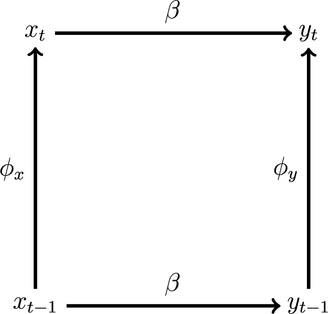
Figure 3. Time-serial Dependence

Figure 4. Cross-Sectional Dependence
This is all familiar: with single-dimensional dependence, purely cross-sectional/spatial or time-serial modeling suffices. However, if both $ {\phi}_y\ne 0 $
and
$ {\phi}_y\ne 0 $
and $ {\rho}_y\ne 0 $
as in Figure 5 so that both temporal and spatial dependence manifest, researchers must model dependence in both dimensions adequately. Omitting/mismodeling spatial dynamics, for example, will leave residual time-serial correlation because the omitted/mismodeled spatial lag yjt
is serially correlated with
$ {\rho}_y\ne 0 $
as in Figure 5 so that both temporal and spatial dependence manifest, researchers must model dependence in both dimensions adequately. Omitting/mismodeling spatial dynamics, for example, will leave residual time-serial correlation because the omitted/mismodeled spatial lag yjt
is serially correlated with $ {y}_{j,t-1} $
, which in turn exhibits that same omitted/mismodeled spatial relation to the included time lag
$ {y}_{j,t-1} $
, which in turn exhibits that same omitted/mismodeled spatial relation to the included time lag $ {y}_{i,t-1} $
. Symmetrically, failing to model temporal dynamics adequately will leave spatial autocorrelation, as the missed aspect of the past,
$ {y}_{i,t-1} $
. Symmetrically, failing to model temporal dynamics adequately will leave spatial autocorrelation, as the missed aspect of the past, $ {y}_{i,t-1} $
, has the same spatial relation to
$ {y}_{i,t-1} $
, has the same spatial relation to $ {y}_{j,t-1} $
as does yit
to the included spatial lag, yjt.
$ {y}_{j,t-1} $
as does yit
to the included spatial lag, yjt.

Figure 5. Space-Time Dependence
To see that spatiotemporal dependence causes bias (OVB) when only one of spatial or temporal dependence is modeled, consider the spatiotemporal-lag model: $ {\mathbf{y}}_t\hskip0.35em =\hskip0.35em \beta {\mathbf{x}}_t+\rho {\mathbf{Wy}}_t+\phi {\mathbf{y}}_{t-1}+{\boldsymbol{\varepsilon}}_t $
(which is also Equation 20), as depicted in Figure 5. If the truth is Equation 20 but one omits
$ {\mathbf{y}}_t\hskip0.35em =\hskip0.35em \beta {\mathbf{x}}_t+\rho {\mathbf{Wy}}_t+\phi {\mathbf{y}}_{t-1}+{\boldsymbol{\varepsilon}}_t $
(which is also Equation 20), as depicted in Figure 5. If the truth is Equation 20 but one omits $ \phi {\mathbf{y}}_{t-1} $
to estimate SAR or omits
$ \phi {\mathbf{y}}_{t-1} $
to estimate SAR or omits $ \rho {\mathbf{Wy}}_t $
to estimate LDV, then OVB arises if
$ \rho {\mathbf{Wy}}_t $
to estimate LDV, then OVB arises if $ \rho \phi \mathrm{Cov}\left({\mathbf{Wy}}_t,{\mathbf{y}}_{t-1}\right)\ne 0 $
. This covariance is necessarily nonzero because spatial dependence implies
$ \rho \phi \mathrm{Cov}\left({\mathbf{Wy}}_t,{\mathbf{y}}_{t-1}\right)\ne 0 $
. This covariance is necessarily nonzero because spatial dependence implies $ {\mathbf{Wy}}_t\leftrightarrow {\mathbf{y}}_t $
and temporal dependence implies
$ {\mathbf{Wy}}_t\leftrightarrow {\mathbf{y}}_t $
and temporal dependence implies $ {\mathbf{y}}_{t-1}\to {\mathbf{y}}_t $
, so
$ {\mathbf{y}}_{t-1}\to {\mathbf{y}}_t $
, so $ {\mathbf{y}}_{t-1}\to {\mathbf{y}}_t\leftrightarrow {\mathbf{Wy}}_t, $
meaning that
$ {\mathbf{y}}_{t-1}\to {\mathbf{y}}_t\leftrightarrow {\mathbf{Wy}}_t, $
meaning that $ \mathrm{Cov}\left({\mathbf{Wy}}_t,{\mathbf{y}}_{t-1}\right)\hskip0.35em =\hskip0.35em \mathrm{Cov}\left(f\left({\mathbf{y}}_t\right),{\mathbf{y}}_{t-1}\right)\ne 0 $
. The sign and magnitude of these OVB can be seen in Achen’s (Reference Achen2000) derivation of the biased
$ \mathrm{Cov}\left({\mathbf{Wy}}_t,{\mathbf{y}}_{t-1}\right)\hskip0.35em =\hskip0.35em \mathrm{Cov}\left(f\left({\mathbf{y}}_t\right),{\mathbf{y}}_{t-1}\right)\ne 0 $
. The sign and magnitude of these OVB can be seen in Achen’s (Reference Achen2000) derivation of the biased $ {\hat{\phi}}_y $
and
$ {\hat{\phi}}_y $
and $ \hat{\beta} $
in an LDV model when additional, unmodeled dynamics
$ \hat{\beta} $
in an LDV model when additional, unmodeled dynamics $ {\phi}_e $
remain in the residual:
$ {\phi}_e $
remain in the residual:
 $$ \mathrm{plim}\;{\hat{\phi}}_y\hskip0.35em =\hskip0.35em {\phi}_y+\left[\frac{\phi_e{\sigma}^2}{\left(1-{\phi}_e{\phi}_y\right){s}^2}\right], $$
and
 $$ \mathrm{plim}\;\hat{\beta}\hskip0.35em =\hskip0.35em \left[1-\frac{\phi_xg}{1-{\phi}_x{\phi}_y}\right]\beta, $$
where $ {s}^2\hskip0.35em =\hskip0.35em {\sigma}_{y_{t-1},x}^2 $
and
$ {s}^2\hskip0.35em =\hskip0.35em {\sigma}_{y_{t-1},x}^2 $
and $ g\hskip0.35em =\hskip0.35em plim\left({\hat{\phi}}_y\right)-{\phi}_y $
(see also Keele and Kelly Reference Keele and Kelly2006). As Achen (Reference Achen2000) notes, any
$ g\hskip0.35em =\hskip0.35em plim\left({\hat{\phi}}_y\right)-{\phi}_y $
(see also Keele and Kelly Reference Keele and Kelly2006). As Achen (Reference Achen2000) notes, any $ {\phi}_e>0 $
inflates
$ {\phi}_e>0 $
inflates $ {\hat{\phi}}_y $
and attenuates
$ {\hat{\phi}}_y $
and attenuates $ \hat{\beta} $
estimates, and as just proven, any unmodeled spatial dependence necessarily produces precisely these same conditions because
$ \hat{\beta} $
estimates, and as just proven, any unmodeled spatial dependence necessarily produces precisely these same conditions because $ {y}_{i,t}\hskip0.35em =\hskip0.35em {\phi}_y{y}_{i,t-1} + {x}_{i,t}\beta +{u}_{i,t}{y}_{\hskip-.05em j,t}\hskip0.35em =\hskip0.35em {\phi}_y{y}_{\hskip-.05em j,t-1}+{x}_{\hskip-.05em j,t}\beta +{u}_{\hskip-.01em j,t}. $
Therefore, any
$ {y}_{i,t}\hskip0.35em =\hskip0.35em {\phi}_y{y}_{i,t-1} + {x}_{i,t}\beta +{u}_{i,t}{y}_{\hskip-.05em j,t}\hskip0.35em =\hskip0.35em {\phi}_y{y}_{\hskip-.05em j,t-1}+{x}_{\hskip-.05em j,t}\beta +{u}_{\hskip-.01em j,t}. $
Therefore, any $ {\rho}_y\ne 0 $
produces
$ {\rho}_y\ne 0 $
produces $ {\phi}_e>0 $
and “Achen’s LDV-bias” manifests. By the usual OVB logic, it follows also that omission or underestimation of
$ {\phi}_e>0 $
and “Achen’s LDV-bias” manifests. By the usual OVB logic, it follows also that omission or underestimation of $ {\rho}_y $
induces primarily overestimation (inflation bias) of
$ {\rho}_y $
induces primarily overestimation (inflation bias) of $ {\hat{\phi}}_y $
, being the coefficient on the included regressor most related to the omitted/mismeasured Wy, and those two biases in turn induce partially compensatory bias of
$ {\hat{\phi}}_y $
, being the coefficient on the included regressor most related to the omitted/mismeasured Wy, and those two biases in turn induce partially compensatory bias of $ {\hat{\beta}}_x $
, with the resultant direction depending on whether the spatial or temporal dependence in x is stronger and resembles more-closely those dependencies in y.
$ {\hat{\beta}}_x $
, with the resultant direction depending on whether the spatial or temporal dependence in x is stronger and resembles more-closely those dependencies in y.
These biases arise because, in TSCS analysis with temporal dependence modeled but spatial dependence excluded, for instance, the factor among the included that is most like the omitted “today’s democracy abroad”—say German democracy today, yj,t
, as omitted explanator of French democracy today, yi,t
—is “yesterday’s democracy at home”—that is, French democracy yesterday, time-lagged $ {y}_{i,t-1} $
. Intuitively, this is because insofar as, “Germany yesterday” relates to “France yesterday”—spatial dependence is present—and “Germany yesterday” relates to “Germany today”—temporal dependence is also present—the omitted “Germany today” relates to the included “France yesterday”. Of course, all of the analogous holds also in the other direction, regarding the omission or relatively inadequate address of temporal dependence.Footnote
20
$ {y}_{i,t-1} $
. Intuitively, this is because insofar as, “Germany yesterday” relates to “France yesterday”—spatial dependence is present—and “Germany yesterday” relates to “Germany today”—temporal dependence is also present—the omitted “Germany today” relates to the included “France yesterday”. Of course, all of the analogous holds also in the other direction, regarding the omission or relatively inadequate address of temporal dependence.Footnote
20
In sum, even if Stimson’s (Reference Stimson1985) “inherent” temporal autocorrelation is accurately modeled, misspecification of the spatial dynamics sets off a chain of biases: the primary attenuation bias (or “zeroing” if omitted) of $ {\rho}_y $
induces overestimation/inflation bias (OVB) of
$ {\rho}_y $
induces overestimation/inflation bias (OVB) of $ {\phi}_y $
, which combine to induce misestimation of
$ {\phi}_y $
, which combine to induce misestimation of $ {\beta}_x $
, usually attenuation because temporal dependence is generally stronger than spatial. Naturally, these biased coefficient estimates mean any related causal-inference tests are biased too, as are estimates of the dynamic and total causal effects of x on y. Specifically regarding effect estimates, typically, the initial “impulses” from x to y (
$ {\beta}_x $
, usually attenuation because temporal dependence is generally stronger than spatial. Naturally, these biased coefficient estimates mean any related causal-inference tests are biased too, as are estimates of the dynamic and total causal effects of x on y. Specifically regarding effect estimates, typically, the initial “impulses” from x to y ( $ {\beta}_x $
) are underestimated and the spatiotemporal dynamics misconstrued as “too-persistent” if spatial dependence is the mismodeled process and, conversely, initial impulses overestimated and spatiotemporal dynamics “too-contagious” if temporal dependence is the mismodeled process. In either case, long-run steady-state effect estimates are biased also.
$ {\beta}_x $
) are underestimated and the spatiotemporal dynamics misconstrued as “too-persistent” if spatial dependence is the mismodeled process and, conversely, initial impulses overestimated and spatiotemporal dynamics “too-contagious” if temporal dependence is the mismodeled process. In either case, long-run steady-state effect estimates are biased also.
Given that inadequate address of spatiotemporal dependence will bias inferential tests and estimates of coefficients, dynamics, and steady-state effects, even researchers for whom spatiotemporal dynamics and dependencies are a nuisance cannot neglect giving them their careful attention. Furthermore, these biases induced by relative neglect of spatial or, less commonly, temporal dependence are of central substantive-theoretical importance as well. In our development-and-democracy terms, relative inadequacy in addressing spatial dependence—inadequate account in the model that, and by what process, democracy clusters—yields estimates that imply inaccurately greater temporal persistence of democracy—for example, an overestimate of democratic-institutionalization and democratic-consolidation effects. If democratic persistence derives from a temporally autoregressive process as such arguments imply, this overestimated temporal dependence will mean smaller immediate-effect estimates—that is, smaller $ {\hat{\beta}}_x $
, with slower decay and so larger long-run-steady-state multipliers in other covariates’ effects on democracy. Beyond these misestimated dynamic and steady-state effects, the biased
$ {\hat{\beta}}_x $
, with slower decay and so larger long-run-steady-state multipliers in other covariates’ effects on democracy. Beyond these misestimated dynamic and steady-state effects, the biased $ {\hat{\beta}}_x $
means that hypothesis tests about the effects of x on y will be biased too, likely increasing false negatives (failure to reject when should).Footnote
21
$ {\hat{\beta}}_x $
means that hypothesis tests about the effects of x on y will be biased too, likely increasing false negatives (failure to reject when should).Footnote
21
Applied researchers also commonly deploy unit and/or period fixed effects to account for spatial or temporal dependence. Unit or period dummies or random effects do address particular forms of spatiotemporal dependence (Elhorst Reference Elhorst2014), but they often fail to adequately capture the spatiotemporal dependence typically present in TSCS data. Unit indicators absorb long-run, fixed or constant, spatial clustering in outcomes, plus any other time-invariant unmodeled unit-specific factors. However, these captured “effects” are additive mean shifts, time-invariant clustering, and not autoregressive or distributed-lag in form. Unit-specific effects also cannot account time-varying unmodeled effects, such as evolving spatially clustered sociocultural or institutional factors. Analogously, period fixed effects/time-dummies account for spatially invariant, uniform shocks common across all units. These too are fixed, additive mean shifts, and so they cannot well-account autoregressive or distributed-lag processes or unit or regional variation in clustered additive shocks, such as influences diffusing among members of regional organizations.
Finally, given the substantively and statistically critical importance of adequately addressing spatiotemporal dependence, researchers will want to conduct appropriate and effective specification testing. In principle, one can conduct specification searches from specific-to-general, starting with sparse spatiotemporal models and determining, using Lagrange-Multiplier (LM) tests, whether to add spatiotemporal-lag terms, or general-to-specific (Hendry Reference Hendry1995), starting with a more-general specification and using Wald or likelihood-ratio (LR) tests to decide whether some spatiotemporal-lag terms may safely be omitted. However, in practice in this context, LM tests of underspecified models will have power against incorrect alternatives (Anselin Reference Anselin1988): for example, LM tests may reject the nonspatial model indicating missing spatial lag y (SAR) or spatial-lag error (SEM) when actually temporal dependence is the missing/poorly-specified process. LM tests can be adjusted using cross-partial gradients of the fuller-specification likelihood to prevent such false/misleading rejections, but these robust-LM tests (Anselin et al. Reference Anselin, Bera, Florax and Yoon1996) as-yet exist for very few combinations of spatiotemporal processes. Instead, we suggest the (first-order) spatiotemporal autoregressive-distributed-lag (STADL) model as a convenient and effective more-general starting point (see Footnote footnote 6), and “testing down.” Researchers can test down using either Wald tests or fit statistics and loss-of-fit tests, such as likelihood and LR tests (Juhl Reference Juhl2021) or R
2 and F-tests of $ \Delta {R}^2 $
, but fit-testing may be preferred given that Wald-testing can be sensitive to reparameterization.Footnote
22
Perhaps better still, researchers can use Akaike or Bayesian–Schwartz Information Criteria (AIC or BIC) fit statistics, which penalize more appropriately for degrees of freedom consumed/excess paramterization than do LR or F and also enable nonnested model comparison, the latter being particularly important given the many alternative models contained within STADL to compare.
$ \Delta {R}^2 $
, but fit-testing may be preferred given that Wald-testing can be sensitive to reparameterization.Footnote
22
Perhaps better still, researchers can use Akaike or Bayesian–Schwartz Information Criteria (AIC or BIC) fit statistics, which penalize more appropriately for degrees of freedom consumed/excess paramterization than do LR or F and also enable nonnested model comparison, the latter being particularly important given the many alternative models contained within STADL to compare.
In summary, as we will further demonstrate by simulation and in reanalyses of real-world applications below, TSCS analyses that relatively neglect spatial (temporal) dependence will estimate greater temporal (spatial) dependence than is actually present and correspondingly misestimate spatiotemporal dynamic and cumulative effects, yielding biased tests and erroneous inferences regarding substantive theoretical propositions. The more-general STADL model offers an effective alternative for applied TSCS analyses.
The STADL Model
The workhorse cross-sectional and time-serial models from spatial and time-series econometrics were introduced above. To review compactly, the baseline spatial-econometric models correspond to the different potential sources for observed spatial association: nonspatial models (NON) for spatially clustered exogenous covariates (including fixed effects), spatial error (SEM) for clustering in unobservables, spatially lagged covariates (SLX) for exogenous spillovers/externalities, and spatial-lag/spatial-autoregressive (SAR) models for endogenous contagion/interdependence:
 $$ {\displaystyle \begin{array}{l}\hskip2pc \mathrm{Clustered}\ \mathrm{Covariates}= NON:\\ {}{\mathbf{y}}_t={\mathbf{x}}_t\beta +{\boldsymbol{\varepsilon}}_t,\mathrm{with}\;{\mathbf{x}}_t\;\mathrm{spatially}\ \mathrm{correlated}.\ \end{array}} $$
 $$ {\displaystyle \begin{array}{l}\mathrm{Clustered}\ \mathrm{Unobservables}= SEM:\\ {}{\mathbf{y}}_t={\mathbf{x}}_t\beta +{\mathbf{u}}_t,\mathrm{with}\;{\mathbf{u}}_t=\lambda {\mathbf{Wu}}_t+{\boldsymbol{\varepsilon}}_t.\end{array}} $$
 $$ {\displaystyle \begin{array}{l}\mathrm{Spillovers}/\mathrm{Externalities}\hskip0.35em =\hskip0.35em SLX:\\ {}\hskip2pc {\mathbf{y}}_t\hskip0.35em =\hskip0.35em {\mathbf{x}}_t\beta +{\mathbf{Wx}}_t\theta +{\boldsymbol{\varepsilon}}_t.\end{array}} $$
 $$ {\displaystyle \begin{array}{l}\mathrm{Interdependence}/\mathrm{Contagion}\hskip0.35em =\hskip0.35em SAR:\\ {}\hskip2pc {\mathbf{y}}_t\hskip0.35em =\hskip0.35em \rho {\mathbf{Wy}}_t+{\mathbf{x}}_t\beta +{\boldsymbol{\varepsilon}}_t.\end{array}} $$
Vectors y
t, x
t, and
ε
t
are N × 1; the matrix W is N × N. Notice, crucially, that “the effect of x” differs importantly across these models/sources/processes. With clustered exogenous covariates (NON), $ \frac{dy_{it}}{dx_{it}}\hskip0.35em =\hskip0.35em \beta $
, and
$ \frac{dy_{it}}{dx_{it}}\hskip0.35em =\hskip0.35em \beta $
, and $ \frac{dy_{js}}{dx_{it}}\hskip0.35em =\hskip0.35em 0\hskip0.20em \forall \hskip0.15em j\ne i,s\ne t $
. Likewise with spatial dependence confined to the orthogonal unobserved component (SEM), the effect of x on y is merely
$ \frac{dy_{js}}{dx_{it}}\hskip0.35em =\hskip0.35em 0\hskip0.20em \forall \hskip0.15em j\ne i,s\ne t $
. Likewise with spatial dependence confined to the orthogonal unobserved component (SEM), the effect of x on y is merely $ \frac{dy_{it}}{dx_{it}}\hskip0.35em =\hskip0.35em \beta $
, and
$ \frac{dy_{it}}{dx_{it}}\hskip0.35em =\hskip0.35em \beta $
, and $ \frac{dy_{js}}{dx_{it}}\hskip0.35em =\hskip0.35em 0\ \forall \hskip0.15em j\ne i,s\ne t $
. In both of these models, with respect to the effect of x on y, “What happens in France stays in France.” With exogenous externalities—that is, in the spatial distributed-lag model (SLX)—“What happens in France spills over into Germany (and France’s other first-order neighbors according to W),” and the story ends there: d
y = W ⋅ d
x
t
⋅ θ + d
x
t
⋅ β. Notice that both the hypothetical/counterfactual, d
x
t, and the effect, d
y
t, are vectors, not scalars: with spatial spillovers, the effect of x differs depending on which units are shocked, and these effects manifest not only in yi
of the shocked unit(s) but also in their first-order neighbors.Footnote
23
In the spatial-autoregressive (SAR) model corresponding to interdependent/contagious contexts, “What happens in France also influences Germany and France’s other neighbors, which in turn influence their neighbors, including France, which influences those neighbors’ neighbors’ neighbors, including Germany again, and so on,” with the effect of d
x
t on y
t reverberating outward and back thusly in an exponentiating series:
$ \frac{dy_{js}}{dx_{it}}\hskip0.35em =\hskip0.35em 0\ \forall \hskip0.15em j\ne i,s\ne t $
. In both of these models, with respect to the effect of x on y, “What happens in France stays in France.” With exogenous externalities—that is, in the spatial distributed-lag model (SLX)—“What happens in France spills over into Germany (and France’s other first-order neighbors according to W),” and the story ends there: d
y = W ⋅ d
x
t
⋅ θ + d
x
t
⋅ β. Notice that both the hypothetical/counterfactual, d
x
t, and the effect, d
y
t, are vectors, not scalars: with spatial spillovers, the effect of x differs depending on which units are shocked, and these effects manifest not only in yi
of the shocked unit(s) but also in their first-order neighbors.Footnote
23
In the spatial-autoregressive (SAR) model corresponding to interdependent/contagious contexts, “What happens in France also influences Germany and France’s other neighbors, which in turn influence their neighbors, including France, which influences those neighbors’ neighbors’ neighbors, including Germany again, and so on,” with the effect of d
x
t on y
t reverberating outward and back thusly in an exponentiating series:
 $$ \begin{align}{\displaystyle \begin{array}{l}d{\mathbf{y}}_t\\ =\Bigg(\underset{\mathrm{self}}{\underbrace{\mathbf{I}}}+\underset{\mathrm{neighbors}}{\underbrace{\rho \mathbf{W}}}+\underset{\mathrm{neighbors}'\mathrm{neighbors}}{\underbrace{\rho^2{\mathbf{W}}^2}}+\underset{\mathrm{neighs}'\mathrm{neighs}'\mathrm{neighs}}{\underbrace{\rho^3{\mathbf{W}}^3}}+\underset{{\mathrm{neighbors}}^4}{\underbrace{\rho^4{\mathbf{W}}^4}}+\dots \Bigg)\cdot d{\mathbf{x}}_t\cdot \beta \\ =\left(\sum \limits_{m=0}^{\infty }{\rho}^m{\mathbf{W}}^m\right)\cdot d{\mathbf{x}}_t\cdot \beta \hskip0.35em =\hskip-0.15em \underset{\mathrm{spatial}\ \mathrm{multiplier}}{\underbrace{{\left(\mathbf{I}-\rho \mathbf{W}\right)}^{-1}}}\cdot \underset{\mathrm{shock}}{\underbrace{d{\mathbf{x}}_t}}\cdot \underset{\mathrm{impulse}}{\underbrace{\beta}}\end{array}} \end{align}$$
Again, insofar as researchers omit or misspecify the spatial-dependence process, say Wy, $ \rho $
is underestimated (
$ \rho $
is underestimated ( $ \hat{\rho}\hskip0.35em =\hskip0.35em 0 $
if omitted), and the OVB formula and intuition implies inflated
$ \hat{\rho}\hskip0.35em =\hskip0.35em 0 $
if omitted), and the OVB formula and intuition implies inflated $ \hat{\beta} $
, with those biases distributed proportionately across the
$ \hat{\beta} $
, with those biases distributed proportionately across the $ {\hat{\beta}}_x $
according to those x’s partial association with the misspecified/omitted Wy, meaning larger induced biases will accrue to the
$ {\hat{\beta}}_x $
according to those x’s partial association with the misspecified/omitted Wy, meaning larger induced biases will accrue to the $ {\hat{\beta}}_x $
whose x cluster spatially more similarly to the pattern implied by W.
$ {\hat{\beta}}_x $
whose x cluster spatially more similarly to the pattern implied by W.
The time-series analogs, also first-order, are compactly expressed using the lag operator, $ {L}^s{y}_t\equiv {y}_{t-s}\forall t>s $
, or the matrix equivalent, Ly
t
(see Footnote footnote 26), as the serially correlated errors (SCE), finite distributed lag (FDL), and lagged dependent variable (LDV) models, along with the static model (StM) with serially correlated exogenous covariates, including time-period fixed effects:
$ {L}^s{y}_t\equiv {y}_{t-s}\forall t>s $
, or the matrix equivalent, Ly
t
(see Footnote footnote 26), as the serially correlated errors (SCE), finite distributed lag (FDL), and lagged dependent variable (LDV) models, along with the static model (StM) with serially correlated exogenous covariates, including time-period fixed effects:
 $$ StM:{\mathbf{y}}_t\hskip0.35em =\hskip0.35em {\mathbf{x}}_t\beta +{\mathbf{u}}_t,\mathrm{with}\;{\mathbf{x}}_t\;\mathrm{serially}\ \mathrm{correlated}. $$
 $$ \hskip-4.45em SCE:{\mathbf{y}}_t\hskip0.35em =\hskip0.35em {\mathbf{x}}_t\beta +{\mathbf{u}}_t,\mathrm{with}\;{\mathbf{u}}_t\hskip0.35em =\hskip0.35em \delta {\mathbf{Lu}}_t+{\boldsymbol{\varepsilon}}_t. $$
 $$ \hskip-10.2em FDL:{\mathbf{y}}_t\hskip0.35em =\hskip0.35em {\mathbf{x}}_t\beta +{\mathbf{Lx}}_t\gamma +{\boldsymbol{\varepsilon}}_t. $$
 $$ \hskip-10.3em LDV:{\mathbf{y}}_t\hskip0.35em =\hskip0.35em \phi {\mathbf{Ly}}_t+{\mathbf{x}}_t\beta +{\boldsymbol{\varepsilon}}_t. $$
Notice again the dynamics, or lack thereof, of the effects of x on y in these time-series models. In the static and serially correlated errors models, the effect of xt
is confined to yt
; there are no temporal dynamics: $ \frac{dy_t}{dx_t}\hskip0.35em =\hskip0.35em \beta \hskip0.3em \mathrm{and}\hskip0.3em \frac{dy_s}{dx_t}\hskip0.35em =\hskip0.35em 0\hskip0.35em \forall\ s\ne t $
. In distributed-lag or autoregressive processes, contrarily, and again paralleling the spatial case, we need first specify dx when? and expand our question to be about the effect on y when? In the distributed-lag case, the effects of x simply spill forward the number of periods equal to the lag-order,
$ \frac{dy_t}{dx_t}\hskip0.35em =\hskip0.35em \beta \hskip0.3em \mathrm{and}\hskip0.3em \frac{dy_s}{dx_t}\hskip0.35em =\hskip0.35em 0\hskip0.35em \forall\ s\ne t $
. In distributed-lag or autoregressive processes, contrarily, and again paralleling the spatial case, we need first specify dx when? and expand our question to be about the effect on y when? In the distributed-lag case, the effects of x simply spill forward the number of periods equal to the lag-order, $ d{\mathbf{y}}_t\hskip0.35em =\hskip0.35em \mathbf{L} $ $ \cdot $ $ d{\mathbf{x}}_t\cdot \beta $
, and are completely dissipated beyond that:
$ d{\mathbf{x}}_t\cdot \beta $
, and are completely dissipated beyond that: $ \frac{d{\mathbf{y}}_{t+s}}{d{\mathbf{x}}_t}\hskip0.35em =\hskip0.35em 0\hskip0.35em \forall\ s>p $
. Temporally autoregressive processes, finally, imply exponentiating decay for temporary shocks, or decaying accumulation for permanent shocks, of long-run steady-state effects going forward infinitely in time, like so:
$ \frac{d{\mathbf{y}}_{t+s}}{d{\mathbf{x}}_t}\hskip0.35em =\hskip0.35em 0\hskip0.35em \forall\ s>p $
. Temporally autoregressive processes, finally, imply exponentiating decay for temporary shocks, or decaying accumulation for permanent shocks, of long-run steady-state effects going forward infinitely in time, like so:
 $$ {\displaystyle \begin{array}{rcl}\underset{\begin{array}{l}\hskip0.24em \mathrm{LRSS}\\ {}\mathrm{response}\end{array}}{\underbrace{dy_{\infty }}}& =& \underset{\mathrm{period}\;0}{\underbrace{\beta dx}}+\underset{\mathrm{period}\;1}{\underbrace{\phi \beta dx}}+\underset{\mathrm{period}\;2}{\underbrace{\phi^2\beta dx}}+\underset{\mathrm{period}\;3}{\underbrace{\phi^3\beta dx}}+\dots \\ {}& =& \underset{\mathrm{if}\hskip0.15em 0<\phi <1,\Rightarrow }{\underbrace{\sum \limits_{s=0}^{\infty }{\phi}^s\beta dx}}\\ {}& =& \underset{\mathrm{LR}\;\mathrm{multiplier}}{\underbrace{\left(\frac{1}{1-\phi}\right)}}\times \underset{\mathrm{impulse}}{\underbrace{\beta}}\times \underset{\begin{array}{l}\mathrm{perm}.\ \\ {}\mathrm{shock}\end{array}}{\underbrace{dx}}\end{array}} $$
From these differing expressions of the effects of x on y implied by the range of possible spatial and temporal processes, one can see how omissions or misspecifications of either temporal or spatial dependence will yield inaccurate tests and estimates of the substantive effects of interest.
Given this critical substantive and statistical importance of allowing the estimation model to express the spatiotemporal dependence inherent to TSCS data in the manner that it manifests, we suggest a combined spatiotemporal autoregressive-distributed-lag (STADL) model of order $ \left({sy}^0,{sx}^0,{se}^0;{ty}^1,{tx}^1,{te}^1\right) $
, where the s or t indicate spatial or temporal lag, the y, x, e indicate which terms are lagged, and the superscript indicates the temporal order of the lag.Footnote
24
We recommend labeling only the terms actually used, so STADL(
$ \left({sy}^0,{sx}^0,{se}^0;{ty}^1,{tx}^1,{te}^1\right) $
, where the s or t indicate spatial or temporal lag, the y, x, e indicate which terms are lagged, and the superscript indicates the temporal order of the lag.Footnote
24
We recommend labeling only the terms actually used, so STADL( $ {sy}^0,{ty}^1 $
) would indicate a first-order spatiotemporal-lag model:
$ {sy}^0,{ty}^1 $
) would indicate a first-order spatiotemporal-lag model:
 $$ {\mathbf{y}}_t\hskip0.35em =\hskip0.35em \rho {\mathbf{Wy}}_t+\phi {\mathbf{Ly}}_t+{\mathbf{x}}_t\beta +{\boldsymbol{\varepsilon}}_t, $$
whereas the general version of the STADL( $ {ty}^p,{tx}^q,{te}^r,{sy}^P,{sx}^Q,{sx}^R $
) is
$ {ty}^p,{tx}^q,{te}^r,{sy}^P,{sx}^Q,{sx}^R $
) is
 $$ \hskip-17em {\mathbf{My}}_t = {\mathbf{Fx}}_t+\mathbf{A}{\boldsymbol{\varepsilon}}_t, $$
 $$ \hskip-4.8em \mathbf{M}\equiv \left(\mathbf{I}-{\phi}_1\mathbf{L}-\dots -{\phi}_p{\mathbf{L}}^p-{\rho}_0\mathbf{W}-\dots -{\rho}_{P-1}{\mathbf{W}}^{P-1}\right), $$
 $$ \hskip-1pc \mathbf{F}\equiv \left(\mathbf{I}\beta +\mathbf{L}{\gamma}_1+\dots +{\mathbf{L}}^q{\gamma}_q+\mathbf{W}{\theta}_0+\dots +{\mathbf{W}}^{Q-1}{\theta}_{Q-1}\right), $$
and
 $$ \hskip-2em \mathbf{A}\equiv {\left(\mathbf{I}-{\unicode{x03B4}}_1\mathbf{L}-\dots -{\unicode{x03B4}}_r{\mathbf{L}}^r-{\unicode{x03BB}}_0\mathbf{W}-\dots -{\unicode{x03BB}}_{R-1}{\mathbf{W}}^{R-1}\right)}^{-1}, $$
where, M, F, and A are the space-time filters of the outcome, predictors, and residuals, respectively.Footnote 25
We express a first-order STADL conveniently for interpretation of spatiotemporal effects as
 $$ \hskip-0.75em \mathbf{y}\hskip0.35em =\hskip0.35em \phi \mathbf{L}\mathbf{y}+\rho \mathbf{W}\mathbf{y}+\mathbf{x}\beta +\mathbf{Lx}\gamma +\mathbf{Wx}\theta +{\left(\mathbf{I}-\delta \mathbf{L}-\lambda \mathbf{W}\right)}^{-1}\boldsymbol{\varepsilon}, $$
 $$ \mathbf{y}\hskip0.35em =\hskip0.35em {\left(\mathbf{I}-\phi \mathbf{L}-\rho \mathbf{W}\right)}^{-1}\left(\mathbf{x}\beta +\mathbf{Lx}\gamma +\mathbf{Wx}\theta +{\left(\mathbf{I}-\delta \mathbf{L}-\lambda \mathbf{W}\right)}^{-1}\boldsymbol{\varepsilon} \right), $$
where I, L, and W are NT × NT; y, x, and
ε
are NT × 1; and L creates a one-period time lag of variables it premultiplies.Footnote
26
Recall that in spatiotemporal analyses of the effect of x, one must specify which units are shocked and when—this is the “treatment”—and, correspondingly, the responses or “effects” will be across all units over all time-periods as determined by the spatiotemporal process given in W and L. In time-series analysis, one must specify when shock dx occurs, and the default shocks are temporary, a one-period shock—dx = +1 in period t
0 with x reverting to its previous level thereafter—and permanent—dx = +1 in time t
0 with the higher x persisting infinitely. In spatial analysis, one must specify where $ dx $
occurs, and the analogous defaults are dx = +1 in one unit and dx = +1 in all units. In space-time analysis, the combined spatial and temporal defaults yield four default shocks: {unit-i or all-units}×{1-period or permanent}.Footnote
27
$ dx $
occurs, and the analogous defaults are dx = +1 in one unit and dx = +1 in all units. In space-time analysis, the combined spatial and temporal defaults yield four default shocks: {unit-i or all-units}×{1-period or permanent}.Footnote
27
A convenient way to express Equation 22 for differentiation by x to track responses over time across all units to some series of hypothetical/counterfactual shocks in N units over T periods, is to create a NT × 1 vector, $ d\mathbf{x}, $
containing the desired spatiotemporal series of shocks:
$ d\mathbf{x}, $
containing the desired spatiotemporal series of shocks:
 $$ d\mathbf{y}\hskip0.35em =\hskip0.35em {\left(\mathbf{I}-\phi \mathbf{L}-\rho \mathbf{W}\right)}^{-1}\cdot \left(\mathbf{I}\beta +\mathbf{L}\gamma +\mathbf{W}\theta \right)\cdot d\mathbf{x}. $$
The NT × 1 vector d y gives the response across all N units period-by-period to this series of shocks, d x. So, for instance, the 1-period, 1-unit default shock is a 1 in that unit’s row of the first N × 1 vector and 0 elsewhere. The 1-unit permanent shock repeats this N × 1 vector down T periods. The all-units 1-period shock starts with an N × 1 vector of ones, and all subsequent elements are 0. The all-units permanent shock is an NT × 1 vector of ones. Beyond these defaults, any set of substantive hypothetical/counterfactual shocks across units over time that researchers may wish to consider may simply be entered as that d x. Indeed, multiple columns of hypothetical shocks can be offered and responses calculated at once, with say NT × N matrices d X and d Y. We suggest N columns here to facilitate the scalar summaries of spatial effects that LeSage and Pace (Reference LeSage and Pace2009) call impacts. Working in a single-period cross-section, they suggest a set of shocks across units given by the N × N identity matrix, which corresponds to shocking each unit alone—that is, the 1-unit default shock, one at a time, column-by-column. For TSCS data, the other T - 1 N × N blocks are all-zeros for the 1-period shock, and the I N repeats over all T for the permanent shock. In a cross-section, the average of the diagonal elements of the N × N d Y gives LeSage and Pace’s (Reference LeSage and Pace2009) average direct effect (ADE) of unit on itself, inclusive of spatiotemporal feedback, and the sum of the off-diagonal elements divided by N gives the average indirect effects (AIE), a summary of the spillover effects. With d X just the identity matrix I N , it may be dropped from Equation 23 and the elements of the multiplier times coefficients matrices may simply be summed and averaged in these ways as LeSage and Pace (Reference LeSage and Pace2009) do.
Long-run steady-state (LRSS) responses in all N units to some permanent N × 1 set of shocks, d
x, is found by returning to Equation 22a, setting $ {\mathbf{y}}_{t-1}\hskip0.35em =\hskip0.35em {\mathbf{y}}_t $
and
$ {\mathbf{y}}_{t-1}\hskip0.35em =\hskip0.35em {\mathbf{y}}_t $
and $ {\mathbf{x}}_{t-1}\hskip0.35em =\hskip0.35em {\mathbf{x}}_t $
by definition of LRSS, to obtain
$ {\mathbf{x}}_{t-1}\hskip0.35em =\hskip0.35em {\mathbf{x}}_t $
by definition of LRSS, to obtain
 $$ d\mathbf{y}\hskip0.35em =\hskip0.35em {\left(\mathbf{I}-\phi \mathbf{I}-\rho \mathbf{W}\right)}^{-1}\left(\mathbf{I}\beta +\mathbf{I}\gamma +\mathbf{W}\theta \right)\cdot d\mathbf{x}. $$
Note both the shocks/treatments d
x and responses/effects d
y reference all N × 1 units $ i $
.Footnote
28
$ i $
.Footnote
28
STADL models can be estimated via maximum-likelihood (or Bayesian) methods, with likelihoods (posteriors) given in Elhorst (Reference Elhorst2001) and LeSage and Pace (Reference LeSage and Pace2009) and maximization detailed in Anselin (Reference Anselin1988).Footnote 29 , Footnote 30 Even previous works that discuss spatiotemporal models and their estimation have neither discussed or derived analytically, as above, nor evaluated through simulation as next, the biases from omitting or mismodeling one of the dependence dimensions in estimates of the other dependence parameters, the covariate coefficients, and the dynamic and total effects.
Monte Carlo Analysis of Dynamic TSCS Models
Our Monte Carlo analyses demonstrate that the biases shown analytically above are of substantively important magnitudes in spatiotemporal TSCS data with properties designed to be representative of common political-science application contexts.
Given the combinatorically vast number of STADL-model variations—26 = 64 first-order models alone—we focus on evaluating the two currently most-widely used in political science: LDV and SAR—that is, STADL( $ {ty}^1 $
) and STADL(
$ {ty}^1 $
) and STADL( $ {sy}^0 $
). LDV and SAR model performance under various forms of temporal or spatial dependence is well known, but we know little as yet about how either one-way model performs under spatiotemporal dependence in both dimensions. Therefore, we generate data from a STADL(
$ {sy}^0 $
). LDV and SAR model performance under various forms of temporal or spatial dependence is well known, but we know little as yet about how either one-way model performs under spatiotemporal dependence in both dimensions. Therefore, we generate data from a STADL( $ {sy}^0,{ty}^1 $
)—that is, the first-order spatiotemporal autoregressive model—with the exogenous covariate x also following a STADL(
$ {sy}^0,{ty}^1 $
)—that is, the first-order spatiotemporal autoregressive model—with the exogenous covariate x also following a STADL( $ {sy}^0,{ty}^1 $
) process, for realism and so induced biases will manifest entirely in
$ {sy}^0,{ty}^1 $
) process, for realism and so induced biases will manifest entirely in $ \hat{\beta} $
:
$ \hat{\beta} $
:
 $$ {\mathbf{y}}_t\hskip0.35em =\hskip0.35em {\phi}_y{\mathbf{y}}_{t-1}+{\rho}_y{\mathbf{Wy}}_t+{\mathbf{x}}_t\beta +{\boldsymbol{\varepsilon}}_{\mathbf{y}}, $$
and
 $$ {\mathbf{x}}_t\hskip0.35em =\hskip0.35em {\phi}_x{\mathbf{x}}_{t-1}+{\rho}_x{\mathbf{Wx}}_t+{\boldsymbol{\varepsilon}}_{\mathbf{x}}, $$
with x
0,
ε
y
, and
ε
x
drawn independent standard-normal. To focus comparisons, we fix several conditions across all simulations: N = 50 and T = 20, giving balanced panels with common sampling dimensions (e.g., U.S. states over 20 years); W generated as k-nearest-neighbor binary-contiguity (k = 5), row-normalized, based on xy-coordinate locations for each unit drawn U(0,100); and parameters β=2, $ {\phi}_x\hskip0.35em =\hskip0.35em 0.6 $
, and ρx
=0.3. We vary the strength of temporal,
$ {\phi}_x\hskip0.35em =\hskip0.35em 0.6 $
, and ρx
=0.3. We vary the strength of temporal, $ {\phi}_y, $
and spatial, ρy
, dependence in the outcome y (further design details in the Appendix).Footnote
31
$ {\phi}_y, $
and spatial, ρy
, dependence in the outcome y (further design details in the Appendix).Footnote
31
Figures 6 and 7 present simulation results for the LDV-model estimates. Figure 6 shows that temporal-lag coefficient-estimate $ {\hat{\phi}}_y $
suffers inflation bias for all true spatial-lag coefficients
$ {\hat{\phi}}_y $
suffers inflation bias for all true spatial-lag coefficients $ {\rho}_y>0 $
, with the bias magnitude increasing in both
$ {\rho}_y>0 $
, with the bias magnitude increasing in both $ {\rho}_y $
and
$ {\rho}_y $
and $ {\phi}_y $
. Even when
$ {\phi}_y $
. Even when $ {\phi}_y\hskip0.35em =\hskip0.35em 0 $
, substantial bias obtains—
$ {\phi}_y\hskip0.35em =\hskip0.35em 0 $
, substantial bias obtains— $ {\hat{\phi}}_y $
reaches 0.18 at the modest maximum spatial dependence considered here: ρy
= .3—and this bias grows as
$ {\hat{\phi}}_y $
reaches 0.18 at the modest maximum spatial dependence considered here: ρy
= .3—and this bias grows as $ {\phi}_y $
increases, the very condition making account of temporal dependence more important. The intuition is simple: the modeled temporal dependence can partially compensate for the missing (or, by extension, mismodeled) spatial dependence, in omitted-variable-bias fashion.
$ {\phi}_y $
increases, the very condition making account of temporal dependence more important. The intuition is simple: the modeled temporal dependence can partially compensate for the missing (or, by extension, mismodeled) spatial dependence, in omitted-variable-bias fashion.

Figure 6. LDV Performance with Spatial Dependence—Bias in $ {\hat{\phi}}_y $

Figure 7. LDV Performance with Spatial Dependence—Bias in $ \hat{\beta} $
Although the strength of temporal dependence is important in itself, researchers often have greater interest in $ \hat{\beta} $
for testing and for estimating the effects of covariates x. Figure 7 shows how the inflated
$ \hat{\beta} $
for testing and for estimating the effects of covariates x. Figure 7 shows how the inflated $ {\hat{\phi}}_y $
estimate generally attenuates the
$ {\hat{\phi}}_y $
estimate generally attenuates the $ \hat{\beta} $
estimate, with this induced attenuation bias also quite sizable and increasing in ρy
and
$ \hat{\beta} $
estimate, with this induced attenuation bias also quite sizable and increasing in ρy
and $ {\phi}_y $
. This is striking given that, with ρy
> 0 and
$ {\phi}_y $
. This is striking given that, with ρy
> 0 and $ \mathrm{Cov}\left(\mathbf{x},\mathbf{Wy}\right)>0 $
, textbook discussion on omitting the spatial lag indicates inflationary OVB in
$ \mathrm{Cov}\left(\mathbf{x},\mathbf{Wy}\right)>0 $
, textbook discussion on omitting the spatial lag indicates inflationary OVB in $ \hat{\beta} $
. The opposite obtains here because that textbook inflationary bias manifests so strongly in
$ \hat{\beta} $
. The opposite obtains here because that textbook inflationary bias manifests so strongly in $ {\hat{\phi}}_y $
as to induce a countervailing deflationary bias in
$ {\hat{\phi}}_y $
as to induce a countervailing deflationary bias in $ \hat{\beta} $
, underscoring how conventional understandings from single-dimensional analyses do not extend straightforwardly to TSCS contexts.Footnote
32
$ \hat{\beta} $
, underscoring how conventional understandings from single-dimensional analyses do not extend straightforwardly to TSCS contexts.Footnote
32
Furthermore, the unmodeled spatial dependence also undermines standard LM tests for serial correlation in the LDV-model estimation residuals, producing an unacceptably high false-positive rate, meaning that using “remaining residual autocorrelation” to assess the adequacy of the LDV in addressing dependence will fail to guide specification properly (see Appendix).
In summary, with spatiotemporal dependence, LDV underestimates the “impulse” effect of xt
, $ \frac{\partial {y}_t}{\partial {x}_t}\hskip0.35em =\hskip0.35em \beta $
, but overestimates
$ \frac{\partial {y}_t}{\partial {x}_t}\hskip0.35em =\hskip0.35em \beta $
, but overestimates $ {\phi}_y $
. Thus, researchers may wonder how well these biases offset in long-run steady-state effect-estimates. In the LDV, the LRSS effect on unit i of permanent dxi
, is
$ {\phi}_y $
. Thus, researchers may wonder how well these biases offset in long-run steady-state effect-estimates. In the LDV, the LRSS effect on unit i of permanent dxi
, is
 $$ \frac{dy_{i, ss}}{dx_i}\hskip0.35em =\hskip0.35em \frac{\beta }{1-{\phi}_y}\;\mathrm{and}\;\frac{dy_{i, ss}}{dx_j}\hskip0.35em =\hskip0.35em 0\hskip0.35em \forall\ j\ne i, $$
whereas the contemporaneous spatial steady-state effect s of one-unit d x on y in the SAR model are
 $$ \frac{d\mathbf{y}}{d\mathbf{x}}\hskip0.35em =\hskip0.35em {\left(\mathbf{I} - \rho \mathbf{W}\right)}^{-1}\beta, $$
which is an N × N matrix of the effects, column-by-column, of dx
i in that column-unit i on y in all units. Thus, the single estimated LRSS effect of x on y from the LDV, or any other nonspatial model, is not even in the correct dimensionality of the spatial effects (plural) of d
x on d
y. As emphasized above, spatial dynamics imply changes in x in any unit have effects across all connected units and changes in x in different units have different effects because units are differently connected to each other. LeSage and Pace’s (Reference LeSage and Pace2009) average direct effects (ADE) scalar summary of the average across i of $ \frac{dx_i}{dy_i} $
, inclusive of spatial dynamics, can be obtained, but even the ADE will not compare closely to the LDV’s LRSS because the LDV’s temporal dynamics are quite imperfect substitutes for SAR’s spatial dynamics.
$ \frac{dx_i}{dy_i} $
, inclusive of spatial dynamics, can be obtained, but even the ADE will not compare closely to the LDV’s LRSS because the LDV’s temporal dynamics are quite imperfect substitutes for SAR’s spatial dynamics.
The correctly spatiotemporal dynamic and LRSS effects of d
X in the general first-order STADL, inclusive of both spatial and temporal dynamics and feedback, are given in Equations 23 and 24. Their simplifications to this STADL( $ {sy}^0,{ty}^1 $
) model are
$ {sy}^0,{ty}^1 $
) model are
 $$ {\displaystyle \begin{array}{l}\mathrm{STADL}\left({\mathrm{sy}}^0,{\mathrm{ty}}^1\right)\;\mathrm{LRSS}\ \mathrm{Effects}:\\ {}\hskip8pt d\mathbf{Y}\hskip0.35em =\hskip0.35em {\left(\mathbf{I}-\phi \mathbf{I}-\rho \mathbf{W}\right)}^{-1}\cdot d\mathbf{X}\cdot \beta, \end{array}} $$
and
 $$ {\displaystyle \begin{array}{l}\mathrm{STADL}\left({\mathrm{sy}}^0,{\mathrm{ty}}^1\right)\;\mathrm{Dynamic}\ \mathrm{Effects}:\\ {}\hskip1em d\mathbf{Y}={\left(\mathbf{I}-\phi \mathbf{L}-\rho \mathbf{W}\right)}^{-1}\cdot d\mathbf{X}\cdot \beta .\end{array}} $$
As explained above, for shocks to one unit at a time, column-by-column, d X is the N × N identity matrix, I N , in the LRSS-effects Equation 28a, and, in the dynamic-effects Equation 28b, d X is that I N stacked vertically T times for permanent shocks, and only in the first N × N block for 1-period shocks. Each (N × 1) column of the resulting d Y in Equation 28a gives the LRSS effects in all N units to shocking the column-unit. In Equation 28b, these N × N blocks of effects in d Y evolve period-by-period T times vertically. The scalar summaries of LRSS or period-by-period ADE and AIE are found by averaging across the N × N effects-block’s diagonals or over all its off-diagonal elements as before. Given all this, clearly, even if the LDV model accurately recovered the LRSS ADE—we will show it does not—it would still produce biased estimates of these unit-specific responses.
Figures 8 and 9 illustrate all this, for single-unit shocks under one set of conditions: $ {\phi}_y\hskip0.35em =\hskip0.35em 0.5 $
and ρy
=0.3. Figure 8 compares the N marginal period-by-period incremental response paths—that is, impulse-response functions, also known as the responses to temporary (1-period) shocks—using Equation 28b of (i) the true STADL model: N gray thinner response-lines, and heavier black response-line average; (ii) the estimated LDV model: one dashed response-line; and (iii) the estimated static-model: one dotted response-line.Footnote
33
Labeled “Direct” are effects of shocks to unit i on outcomes in unit i; “Indirect” are summed responses in units
$ {\phi}_y\hskip0.35em =\hskip0.35em 0.5 $
and ρy
=0.3. Figure 8 compares the N marginal period-by-period incremental response paths—that is, impulse-response functions, also known as the responses to temporary (1-period) shocks—using Equation 28b of (i) the true STADL model: N gray thinner response-lines, and heavier black response-line average; (ii) the estimated LDV model: one dashed response-line; and (iii) the estimated static-model: one dotted response-line.Footnote
33
Labeled “Direct” are effects of shocks to unit i on outcomes in unit i; “Indirect” are summed responses in units $ j\ne i $
to shocks in unit i; and “Total” sums Direct and Indirect. Figure 9 plots the analogous cumulative response paths to permanent single-unit shocks.Footnote
34
As shown analytically above, the LDV substantially underestimates the contemporaneous effect for all N units, and it overestimates the temporal persistence, giving incorrectly slower decay. Thus, the LDV estimates one smaller, but more-persistent, effect than the true STADL’s heterogeneous, larger, quicker-decaying correct effects. The LDV also overestimates (underestimates) the cumulative LRSS direct (total) effect at 6.41, to which it arrives more slowly, compared with the average cumulative LRSS direct effect of 4.39 and total effect of 10.0 from the correct STADL, to which the STADL responses arrive more quickly. The static model, meanwhile, radically overstates direct (and total) contemporaneous effect and badly mischaracterizes (and understates) the direct (and total) cumulative effects. In sum, even on average—that is, disregarding the unit-specific variation—the LDV model performs poorly, and the static nonspatial model very poorly.
$ j\ne i $
to shocks in unit i; and “Total” sums Direct and Indirect. Figure 9 plots the analogous cumulative response paths to permanent single-unit shocks.Footnote
34
As shown analytically above, the LDV substantially underestimates the contemporaneous effect for all N units, and it overestimates the temporal persistence, giving incorrectly slower decay. Thus, the LDV estimates one smaller, but more-persistent, effect than the true STADL’s heterogeneous, larger, quicker-decaying correct effects. The LDV also overestimates (underestimates) the cumulative LRSS direct (total) effect at 6.41, to which it arrives more slowly, compared with the average cumulative LRSS direct effect of 4.39 and total effect of 10.0 from the correct STADL, to which the STADL responses arrive more quickly. The static model, meanwhile, radically overstates direct (and total) contemporaneous effect and badly mischaracterizes (and understates) the direct (and total) cumulative effects. In sum, even on average—that is, disregarding the unit-specific variation—the LDV model performs poorly, and the static nonspatial model very poorly.

Figure 8. Response-Path Estimates of LDV Model with Spatial Dependence
Note: dotted line = Static; dashed line = LDV; gray lines = STADL unit-by-unit; black line = STADL average.

Figure 9. Cumulative Response-Path Estimates of LDV Model with Spatial Dependence
Note: dotted line = Static; dashed line = LDV; gray lines = STADL unit-by-unit; black line = STADL average.
The analogous explorations of SAR-model estimation performance show (Figure 10) the expected inflation bias in $ {\hat{\rho}}_y $
when temporal dependence is present but unmodeled. When
$ {\hat{\rho}}_y $
when temporal dependence is present but unmodeled. When $ {\phi}_y\hskip0.35em =\hskip0.35em 0.5 $
, for example, the
$ {\phi}_y\hskip0.35em =\hskip0.35em 0.5 $
, for example, the $ {\hat{\rho}}_y $
estimates from the SAR model average more than two times (!) the true value of
$ {\hat{\rho}}_y $
estimates from the SAR model average more than two times (!) the true value of $ {\rho}_y $
. As researchers more commonly attach theoretic importance to their spatial-dependence specifications than to temporal dependence—selecting connectivity matrices to test competing theories of diffusion, for example—this is per se more substantively concerning than in the LDV case. Researchers interested in evaluating spatial theories must attend equally highly carefully to accurately modeling temporal dynamics. Even with spatial processes well-specified, and W and the spatial-lag terms correct and well-measured in the model, failing to adequately address temporal dependence can produce wildly inaccurate understandings of the spatial processes actually operating in the data.Footnote
35
$ {\rho}_y $
. As researchers more commonly attach theoretic importance to their spatial-dependence specifications than to temporal dependence—selecting connectivity matrices to test competing theories of diffusion, for example—this is per se more substantively concerning than in the LDV case. Researchers interested in evaluating spatial theories must attend equally highly carefully to accurately modeling temporal dynamics. Even with spatial processes well-specified, and W and the spatial-lag terms correct and well-measured in the model, failing to adequately address temporal dependence can produce wildly inaccurate understandings of the spatial processes actually operating in the data.Footnote
35

Figure 10. SAR Performance with Temporal Dependence—Bias in ρ y
Regarding $ \hat{\beta} $
, Figure 11 reveals the expected inflationary bias from failing to model temporal dependence, and this bias increases in the unmodeled
$ \hat{\beta} $
, Figure 11 reveals the expected inflationary bias from failing to model temporal dependence, and this bias increases in the unmodeled $ {\phi}_y $
. However, this bias does not also increase with ρy. Why? First, temporal dependence often, as in our simulation, far exceeds spatial dependence. Therefore, the inflationary bias in
$ {\phi}_y $
. However, this bias does not also increase with ρy. Why? First, temporal dependence often, as in our simulation, far exceeds spatial dependence. Therefore, the inflationary bias in $ \hat{\beta} $
from the unmodeled temporal dynamics weighs more heavily against the downward bias from overestimated
$ \hat{\beta} $
from the unmodeled temporal dynamics weighs more heavily against the downward bias from overestimated $ {\hat{\rho}}_y $
than in the reverse scenario. Second, our simulation parameters, again realistically, set x also to manifest greater temporal than spatial dependence:
$ {\hat{\rho}}_y $
than in the reverse scenario. Second, our simulation parameters, again realistically, set x also to manifest greater temporal than spatial dependence: $ {\phi}_x\hskip0.35em =\hskip0.35em 0.6 $
versus ρx
= 0.3. Thus, the correlation between
$ {\phi}_x\hskip0.35em =\hskip0.35em 0.6 $
versus ρx
= 0.3. Thus, the correlation between $ {x}_{i,t} $
and
$ {x}_{i,t} $
and $ {y}_{i,t-1} $
, and so the bias from omitting the latter, is greater than the bias induced by overestimating
$ {y}_{i,t-1} $
, and so the bias from omitting the latter, is greater than the bias induced by overestimating $ {\hat{\rho}}_y $
and the correlation of
$ {\hat{\rho}}_y $
and the correlation of $ {x}_{i,t} $
and
$ {x}_{i,t} $
and $ {y}_{j,t} $
.Footnote
36
$ {y}_{j,t} $
.Footnote
36

Figure 11. SAR Performance with Temporal Dependence — Bias in $ \beta $
Although the $ \hat{\beta} $
estimate is inflated in proportion solely to the temporal-dependence misspecification, that bias plus the inflation bias also in
$ \hat{\beta} $
estimate is inflated in proportion solely to the temporal-dependence misspecification, that bias plus the inflation bias also in $ {\hat{\rho}}_y $
seriously compromises the effects estimates. Recall that in spatial-autoregressive models, as in all models beyond the purely linear-additive and separable, the effect of x on y is not β, which is merely the pre-spatiotemporal impulse, but instead the effects are given by Equations 23 and 24. For scalar summaries of these multidimensional effects, we use the average-direct and average-indirect effects, ADE and AIE, described above. Comparing the values estimated by the incorrect SAR with those from the true STADL, we find that SAR overestimates the single-unit-shock responses, SAR ADE = 3.96 versus STADL ADE = 2.03, and radically overestimates the AIE, SAR AIE = 6.76 versus STADL AIE = 0.82, and so the average total effects (ATE), SAR ATE = 10.72 versus STADL ATE = 2.85. Furthermore, despite the absence of temporal dynamics from the estimation model, the long-run steady-state (LRSS) total effects are also modestly overestimated: SAR LRSS ATE = 10.72 versus STADL LRSS ATE = 10.
$ {\hat{\rho}}_y $
seriously compromises the effects estimates. Recall that in spatial-autoregressive models, as in all models beyond the purely linear-additive and separable, the effect of x on y is not β, which is merely the pre-spatiotemporal impulse, but instead the effects are given by Equations 23 and 24. For scalar summaries of these multidimensional effects, we use the average-direct and average-indirect effects, ADE and AIE, described above. Comparing the values estimated by the incorrect SAR with those from the true STADL, we find that SAR overestimates the single-unit-shock responses, SAR ADE = 3.96 versus STADL ADE = 2.03, and radically overestimates the AIE, SAR AIE = 6.76 versus STADL AIE = 0.82, and so the average total effects (ATE), SAR ATE = 10.72 versus STADL ATE = 2.85. Furthermore, despite the absence of temporal dynamics from the estimation model, the long-run steady-state (LRSS) total effects are also modestly overestimated: SAR LRSS ATE = 10.72 versus STADL LRSS ATE = 10.
Empirical Reanalyses
To demonstrate the importance of modeling spatiotemporal dependence appropriately in applied TSCS data analysis, we conduct two brief reanalyses of prominent recent studies. First, we revisit Acemoglu et al. (Reference Acemoglu, Johnson, Robinson and Yared2008) to evaluate empirically the development–democracy connection, our running illustration. Particularly apt for our purposes, they include temporal autoregressive dependence and fixed unit and period effects, but they otherwise neglect spatial dependence. Second, we analyze data from Lührmann, Marquardt, and Mechkova (Reference Lührmann, Marquardt and Mechkova2020), who develop several new country-year indices of vertical, horizontal, and diagonal political accountability, plus an overall accountability index. The article focuses on demonstrating the content, convergent, and construct validity of these measures, but includes analyses of accountability and infant morality in which they account for spatial dependence and include fixed unit and period effects while omitting autoregressive temporal dependence. These reanalyses also nicely parallel our simulation studies: one models temporal dependence while relatively neglecting spatial dependence; the other models spatial dependence while relatively neglecting temporal dependence.
Reanalysis of Acemoglu et al. (Reference Acemoglu, Johnson, Robinson and Yared2008) on Development and Democracy
Acemoglu et al.’s (Reference Acemoglu, Johnson, Robinson and Yared2008) main finding is that the otherwise robust positive relation of economic development with democratization disappears with country fixed effects included. Table 1 reports five models using their data to regress Polity IV Democracy on lagged real GDP per capita (RGDPpc), plus various combinations of fixed effects and autoregressive lags, with column 4 replicating their main two-way-fixed-effects regression. The results starkly highlight how these specification choices affect one’s analysis and inferences.
Table 1. Reanalysis of Development and Democracy in Acemoglu et al. (Reference Acemoglu, Johnson, Robinson and Yared2008)

Note: *p < 0.10, ** p < 0.05, *** p < 0.01.
The column 1 model includes a spatial lag created with a row-standardized nearest-neighbor weights matrix (autogenerated by our tscsdep R package). With this spatial autoregression the only spatiotemporal dependence in model 1, the positive and significant spatial-lag coefficient may be an overestimate. Column 2 adds fixed year-effects. Because democracy trends globally over the sample period, this addition greatly improves model fit: log likelihood increases over 30% (-162.34 to -129.62) and BIC decreases from 351.7 to 340.2. The coefficient estimates are affected only slightly, but notably $ \hat{\rho} $
becomes larger and more significant.
$ \hat{\rho} $
becomes larger and more significant.
Column 3 adds country fixed effects, and column 4 replaces the spatial lag with a temporal lag, the latter replicating Acemoglu et al.’s (Reference Acemoglu, Johnson, Robinson and Yared2008) Table 3, column 2. These results reflect the contribution from their analysis: the statistical significance of the RGDPpc coefficient estimate disappears with country fixed effects added. The spatial-lag coefficient also becomes insignificant in column 3, with the country fixed effects apparently absorbing sizable time-invariant spatial clustering in both RGDPpc and democracy. However, the influence on model fit is less clear. LL improves greatly, but the BIC fit statistic, which penalizes for overparameterizing the model and overfitting the sample, gets much worse, increasing almost 40% (340.2 to 472.3). Scholars can reasonably disagree about the model-selection implications of these comparisons, but BIC strongly indicates that the LL improvement from the country dummies does not merit the 133 degrees of freedom they consume.
Acemoglu et al.’s (Reference Acemoglu, Johnson, Robinson and Yared2008) column 4 model improves on 2 and 3 in terms of both coefficient significance and model fit, underscoring the crucial importance of temporally autoregressive dynamics in democratic development. The final column 5 presents results from the model with by far the best BIC (-406.6) and LL close to model 3 despite 132 fewer estimated parameters. The likelihood-ratio test of Model 5, which includes both temporal and spatial lag, and period fixed effects, versus Model 3 yields a chi-square statistic of 12.06, which with 132 degrees of freedom overwhelmingly fails to reject: $ p\approx 1.0 $
. The STADL(
$ p\approx 1.0 $
. The STADL( $ {s}_y^0,{t}_y^1 $
) plus time dummies model is therefore overwhelmingly preferred by our model-selection criteria. The coefficients on RGDPpc, the temporal lag, and the spatial lag are all statistically significant. The comparison of the STADL
$ {s}_y^0,{t}_y^1 $
) plus time dummies model is therefore overwhelmingly preferred by our model-selection criteria. The coefficients on RGDPpc, the temporal lag, and the spatial lag are all statistically significant. The comparison of the STADL $ \left({s}_y^0,{t}_y^1\right) $
plus time dummies 5 with Acemoglu et al.’s temporally autoregressive two-way fixed-effects model 4 is similar to the comparison of the models in columns 3 and 2: the inclusion of country fixed effects leads to a significant improvement in LL, but if we penalize for overparameterizing and overfitting, the BIC concludes emphatically that the LL increase does not remotely justify the cost in parsimony terms (consumed degrees of freedom).
$ \left({s}_y^0,{t}_y^1\right) $
plus time dummies 5 with Acemoglu et al.’s temporally autoregressive two-way fixed-effects model 4 is similar to the comparison of the models in columns 3 and 2: the inclusion of country fixed effects leads to a significant improvement in LL, but if we penalize for overparameterizing and overfitting, the BIC concludes emphatically that the LL increase does not remotely justify the cost in parsimony terms (consumed degrees of freedom).
Comparing the coefficient estimates across these models also nicely illustrates in real-data application the conclusions drawn above in our analytics and simulations. Failing to include a temporal lag in model 2 results in larger estimates of $ \hat{\rho} $
and
$ \hat{\rho} $
and $ \hat{\beta} $
relative to model 5, where temporal dependence is directly accounted. This parallels our simulations’ findings that SAR (here model 2) suffers inflation bias in
$ \hat{\beta} $
relative to model 5, where temporal dependence is directly accounted. This parallels our simulations’ findings that SAR (here model 2) suffers inflation bias in $ \hat{\rho} $
and
$ \hat{\rho} $
and $ \hat{\beta} $
when temporal dependence is present but unmodeled. In the simulations, the SAR model
$ \hat{\beta} $
when temporal dependence is present but unmodeled. In the simulations, the SAR model $ \hat{\rho} $
averaged about twice the true STADL ρ; similarly here,
$ \hat{\rho} $
averaged about twice the true STADL ρ; similarly here, $ \hat{\rho} $
from model 5 is 0.091, whereas model 2
$ \hat{\rho} $
from model 5 is 0.091, whereas model 2 $ \hat{\rho} $
is roughly 1.8 times larger at 0.167.
$ \hat{\rho} $
is roughly 1.8 times larger at 0.167.
This also has substantively important implications for how development is estimated to affect democracy across space and time. The positive, significant temporal-lag and spatial-lag coefficients in our preferred model 5 indicate that development effects on democracy in one country at one time reverberate autoregressively both forward in time and across countries in space. We can calculate summaries of these average short-run (first-period) and long-run direct, indirect, and total effects (ADE, AIE, ATE) as shown in Equations 28a and 28b. Using model 5 coefficient estimates, a one-unit single-country shock to RGDPpc has contemporaneous ADE of +0.053 on democracy in that same country and AIE of +0.005 on democracy in other countries, for a combined ATE of +0.058. The respective long-run cumulative estimates are LRSS ADE = +0.209, LRSS AIE = +0.021, and LRSS ATE = +0.230. These differ considerably from model (2), where the estimated effects have no temporal dynamics and are instead instantaneous at ADE = +0.237, AIE = +0.036, and ATE = +0.273. Although these latter static SAR-model estimated effects might seem not too dissimilar from the long-run effects from spatiotemporally dynamic STADL model 5—differences of ADE +.028 $ \approx $
13%, AIE + .015
$ \approx $
13%, AIE + .015 $ \approx $
71%, and ATE = +.043
$ \approx $
71%, and ATE = +.043 $ \approx $
19%—the effects from model 2 incur immediately and fully, so the same-country, same-period effects from a change in development on democracy is ADE = +0.053 in model 5 versus ADE = +0.237 in model 2, more than a fourfold (
$ \approx $
19%—the effects from model 2 incur immediately and fully, so the same-country, same-period effects from a change in development on democracy is ADE = +0.053 in model 5 versus ADE = +0.237 in model 2, more than a fourfold ( $ \approx $
447%) difference.
$ \approx $
447%) difference.
In short, the choice of spatiotemporal model dramatically affects one’s conclusions both of whether and of how development relates to democracy.
Reanalysis of Lührmann, Marquardt, and Mechkova (Reference Lührmann, Marquardt and Mechkova2020) on Accountability and Infant Mortality
In their recent APSR article, Lührmann, Marquardt, and Mechkova (Reference Lührmann, Marquardt and Mechkova2020) demonstrate construct validity for their overall index of political accountability (in part) by verifying its negative correlation with infant-mortality rates. They estimate four time-series-cross-sectional regressions, both in isolation and in combination with alternative measures of accountability taken from the World Bank and Freedom House. We reanalyze one of their primary regressions: MODEL 1 in their Figure 8. The model includes the new overall accountability index and a large set of controls, including country and year fixed effects as some account of spatial and temporal dependence, plus a regional-average infant-mortality variable. This regional-average variable is actually a kind of spatial lag, being the average dependent variable among regional neighbors, but it is treated as an exogenous regressor. Beyond the time-period indicators, temporal dependence and dynamics are not modeled.
The country indicators account for fixed (long-run) additive spatial clustering in the outcome, infant mortality rates. Fixed here means constant over the entire sample period (1960–2010). Additive means the clustering manifests as a single mean shift, as opposed to a multiplicative effect on some observed or unobserved covariate or an autoregressive spatially dynamic process. The regional-average variable, which instead gives a spatial-autoregressive process, accounts for potential time-varying (long-run) spatial clustering. If there are multiple regional equilibria over time (e.g., Southeast Asia 1961–1980; Southeast Asia 1981–2000; Southeast Asia 2001–2010), though, the regional-average spatial lag cannot account for this. Country fixed effects cannot either.
The year fixed effects can account for “short-run” (unique year-by-year) common shocks that are global in scope. Again, these are additive: some mean shift each year that is common across all countries. The same infant-mortality shock, equal to that year’s single time-dummy coefficient, hits every country. Year fixed effects cannot account for common shocks that are regional or otherwise subglobal in nature—for example an infant-mortality shock specific to Southeast Asia. If the relevant regions or groups of countries were known preanalysis, regional-period shock indicators (e.g., Southeast Asia 1987) could be included in regression models, but the relevant spatiotemporal units are rarely known, and this strategy quickly overloads degrees of freedom.
An alternative strategy to account for regional common shocks is to add spatial lags in first differences to regression models. Because spatial lags represent autoregression in space—countries influence first-, second-, and third-order (etc.) neighbors with geometrically decaying influence—they provide a certain flexibility with respect to identifying the geographical boundaries of shocks that regional indicators do not. The spatial-weights matrix could connect $ k $
-nearest neighbors—for example, around each country (automatically generated using tscsdep), whereas regions must be preidentified for indicator-variable strategies. Spatial lags are also more parsimonious than regional-period indicators because a single spatial lag defines a “neighborhood” for every sample-unit.
$ k $
-nearest neighbors—for example, around each country (automatically generated using tscsdep), whereas regions must be preidentified for indicator-variable strategies. Spatial lags are also more parsimonious than regional-period indicators because a single spatial lag defines a “neighborhood” for every sample-unit.
More generally, in STADL models, time-differenced right-hand-side variables produce only short-run effects in left-hand-side outcomes, whereas regressors in levels produce long-run effects through temporal multipliers. Lührmann, Marquardt, and Mechkova’s (Reference Lührmann, Marquardt and Mechkova2020) MODEL 1 includes a de facto endogenous spatial lag in the regional averages, which, for our reanalysis purposes, we will retain as an (erroneously) exogenous regressor and will assume to reasonably proxy the true spatial-dependence process. MODEL 1 also includes country and year fixed effects, but no temporal dynamics, a stark omission given that infant-mortality rates are highly persistent temporally. We also think heterogeneous regional infant-mortality shocks are highly plausible. Therefore, we add to our reanalysis model a temporal lag and a time-differenced nearest-neighbor spatial lag:
 $$ {y}_{it}\hskip0.35em =\hskip0.35em {\mathbf{x}}_{it}\beta +\phi {y}_{it-1}+\rho {\mathbf{w}}_i\Delta {\mathbf{y}}_t+{f}_i+{g}_t+{\boldsymbol{\varepsilon}}_{it}, $$
with yit
being infant mortality in unit i in year t, x
it
a 1 × k vector of exogenous covariates for unit-year it, β a k × 1 vector of coefficients, ρ the spatial-lag coefficient, w
i
unit-i’s 1 × N vector of spatial weights on units j, $ \Delta {\mathbf{y}}_t $
the time-t N × 1 vector of differenced outcomes, fi
a fixed-unit effect, gt
a fixed-period effect, and
$ \Delta {\mathbf{y}}_t $
the time-t N × 1 vector of differenced outcomes, fi
a fixed-unit effect, gt
a fixed-period effect, and $ {\boldsymbol{\varepsilon}}_{it} $
an
$ {\boldsymbol{\varepsilon}}_{it} $
an $ i.i.d. $
disturbance for unit-time it. Some algebraic manipulation rewrites this with a differenced outcome (more convenient for expressing the likelihood):
$ i.i.d. $
disturbance for unit-time it. Some algebraic manipulation rewrites this with a differenced outcome (more convenient for expressing the likelihood):
 $$ \Delta {y}_{it}\hskip0.35em =\hskip0.35em {\mathbf{x}}_{it}\beta +\left(\phi -1\right){y}_{it-1}+\rho {\mathbf{w}}_i\Delta {\mathbf{y}}_t+{f}_i+{g}_t+{\boldsymbol{\varepsilon}}_{it}. $$
Although the regional-average variable (treated as exogenous still for comparability) incorporates some spatial dependence, its coefficient is likely overestimated because temporal dependence, likely very high in infant mortality, is omitted, beyond the year effects—and year effects, due to regional concentration in infant-mortality shocks, likely miss considerable spatiotemporal dependence also. Our analyses above suggest that the unfortunate consequence of this misestimation of the spatiotemporal dependence is that Lührmann, Marquardt, and Mechkova (Reference Lührmann, Marquardt and Mechkova2020) may have underestimated the strength of their political-accountability measure’s relationship to infant mortality.
Table 2 column 1 replicates their original results. Then, with tscsdep, we create a nearest-neighbor spatial-weights matrix and estimate the spatiotemporal-autoregressive STADL $ \left({sy}^0,{ty}^1\right) $
model incorporating spatially and temporally lagged dependent-variable regressors, reported in the second column. The LRSS effectsFootnote
37
of each covariate x in xit
are given in the third column. Comparing the implicit spatial steady state implied by the regional-average variable in the original regression, which ignores temporal (autoregressive) dynamics, with our estimate of the spatial steady-state effect, we estimate that the former overstates the extent of spatial dependence by nearly 44% in this comparison. More simply and starkly, comparing the first and third columns, we estimate that the spatiotemporal LRSS effect of Lührmann, Marquardt, and Mechkova’s (Reference Lührmann, Marquardt and Mechkova2020) political accountability on infant mortality rates (
$ \left({sy}^0,{ty}^1\right) $
model incorporating spatially and temporally lagged dependent-variable regressors, reported in the second column. The LRSS effectsFootnote
37
of each covariate x in xit
are given in the third column. Comparing the implicit spatial steady state implied by the regional-average variable in the original regression, which ignores temporal (autoregressive) dynamics, with our estimate of the spatial steady-state effect, we estimate that the former overstates the extent of spatial dependence by nearly 44% in this comparison. More simply and starkly, comparing the first and third columns, we estimate that the spatiotemporal LRSS effect of Lührmann, Marquardt, and Mechkova’s (Reference Lührmann, Marquardt and Mechkova2020) political accountability on infant mortality rates ( $ -9.500 $
) is more than double the effect they reported
$ -9.500 $
) is more than double the effect they reported $ \left(\hat{\beta}\hskip0.35em =\hskip0.35em -4.339\right) $
, which mostly ignores these important spatial and temporal dynamic dependencies. In column 4 (model 3), we drop the country dummies from model 2. In contrast with the analysis in Table 1, we find that the inclusion of country fixed effects here leads to unambiguous improvement in model fit by either LL or BIC. Model 2 is clearly the preferred model among this set.
$ \left(\hat{\beta}\hskip0.35em =\hskip0.35em -4.339\right) $
, which mostly ignores these important spatial and temporal dynamic dependencies. In column 4 (model 3), we drop the country dummies from model 2. In contrast with the analysis in Table 1, we find that the inclusion of country fixed effects here leads to unambiguous improvement in model fit by either LL or BIC. Model 2 is clearly the preferred model among this set.
Table 2. Reanalysis of the Accountability/Infant Mortality Regression in Lührmann, Marquardt, and Mechkova (Reference Lührmann, Marquardt and Mechkova2020)

Note: *p < 0.10, ** p < 0.05, *** p < 0.01.
Conclusion
This paper considers the implications of the multidimensional dependence, dynamics in both space and time, that typically manifests in TSCS data. With both spatial and temporal dependence present, we have shown that modeling dependence in only one dimension while neglecting the other biases estimates of all dependence parameters, usually resulting in inflation bias in the parameter(s) of the included or better-specified dimension. Not only does this risk misunderstandings about whether the observed spatiotemporal patterns are due to temporal or spatial dependence; it can also threaten researchers’ ability to effectively discriminate between competing sources of dependence—dependent outcomes, covariates, or unobservables—along either dimension. These biases in the dependence parameter estimates also induce biases in the covariate coefficient estimates. With these dependence parameter and covariate coefficient estimates both biased, spatiotemporal-dynamic and long-run-steady-state effects are biased too, as are hypothesis tests and inferences made using these estimates. Furthermore, we demonstrate that these estimation biases with dependence in both space and time differ from those considered heretofore in textbook treatments of temporal or spatial dependence alone. For example, usually omitted spatial interdependence results in partially offsetting inflationary bias in the covariate coefficients. However, we showed that in TSCS analyses, if a time-lagged outcome is included in the model, then the inflationary bias from the omitted spatial lag will primarily manifest in this temporal lag, and that in turn induces partially offsetting attenuation in the covariate coefficients. Thus, researchers’ previous methodological understandings, which derived from single-dimensional studies, can sometimes provide poor guidance when analyzing TSCS data.
Given these concerns, we propose that researchers instead use a spatiotemporal model, the first-order STADL, as an effective starting point that nests many of the most-widely used space-time specifications in political science (e.g., the first-order LDV, ADL, SAR, and SDM) and combinations thereof. We suggested that beginning with this more-general STADL specification and using model-restriction tests and goodness-of-fit statistics to guide model refinement reduces the risk of unmodeled dynamics, and so of biased estimation and invalid inferences. Although estimating these models is not significantly more difficult than estimating single-dimensional analogs, interpretation of the results raises considerable challenges because the meanings of both βx
and the calculation of $ \frac{d\mathbf{y}}{d\mathbf{x}} $
changes for different STADL models. Therefore, we have discussed at length the varieties of spatiotemporally dynamic effects that different STADL specifications entail. To better enable researchers to adopt the strategies presented here, we developed R package tscsdep (see Appendix for detail; GitHub to download https://github.com/judechays/STADL) to automate the construction of common weights matrices, W, including for unbalanced panels, estimation of the first-order STADL model, and calculation of STADL dynamic and LRSS effects.
$ \frac{d\mathbf{y}}{d\mathbf{x}} $
changes for different STADL models. Therefore, we have discussed at length the varieties of spatiotemporally dynamic effects that different STADL specifications entail. To better enable researchers to adopt the strategies presented here, we developed R package tscsdep (see Appendix for detail; GitHub to download https://github.com/judechays/STADL) to automate the construction of common weights matrices, W, including for unbalanced panels, estimation of the first-order STADL model, and calculation of STADL dynamic and LRSS effects.
We see several priorities for expanding upon our recommended STADL approach for TSCS data analysis. First, we have not addressed the topic of order specification, focusing instead on source specification. Second, we did not raise the possibility of overfitting STADL models to sample idiosyncrasies. Finally, we have not discussed the implications of measurement error, particularly with respect to W, in spatiotemporally interdependent data. We believe effective approaches to these challenges extend naturally from time-series and spatial econometrics. For instance, autocorrelation and partial autocorrelation (AC, PAC) functions used to guide time-series order specification might be extended to spatiotemporal AC and PAC functions. Likewise, cross-validation and out-of-sample performance are the gold-standard safeguards against overfitting and are similarly extendable to spatiotemporal TSCS contexts. On measurement error, various Bayesian strategies of model averaging (Juhl Reference Juhl2020) and/or combining measurement and estimation models seem most promising to us. These projects head our research agenda going forward.
Supplementary Materials
To view supplementary material for this article, please visit http://doi.org/10.1017/S0003055422000272.
DATA AVAILABILITY STATEMENT
Research documentation and data that support the findings of this study are openly available at the Amercian Political Science Review Dataverse: https://doi.org/10.7910/DVN/DBMJQZ.
ACKNOWLEDGMENTS
We thank the organizers and participants of the workshop conference on “Modeling Politics and Policy in Time and Space” held at Texas A&M University, where the earliest seeds of this research were sown in April 2017. We are also extremely grateful to the editor and three anonymous reviewers for tremendously constructive comments, criticisms, and suggestions.
FUNDING STATEMENT
This research was funded by the National Science Foundation [NSF DMS-1925119 to SJC].
CONFLICT OF INTEREST
The authors declare no ethical issues or conflicts of interest in this research.
ETHICAL STANDARDS
The authors affirm this research did not involve human subjects.


 Open access