


1. Introduction
Perhaps the most fundamentally important statistical description of an irregular sea is the probability density function (PDF) for the surface elevation itself. The positive tail of the PDF is of special importance, as it governs the likelihood of extreme positive surface elevations, typical of rogue waves. In his classical work, Longuet-Higgins (Reference Longuet-Higgins1963) showed that this PDF could be formulated in terms of an integral arising from the cumulant generating function. His formulation is free of assumptions involving narrow-bandedness of the spectrum or small directionality of the wave field. To leading order, the result is Gaussian, whereas Longuet-Higgins (Reference Longuet-Higgins1963) derived approximate Gram–Charlier series solutions for this PDF to second and third order. Recently, the present authors (henceforth referred to as FKZ, Fuhrman, Klahn & Zhai Reference Fuhrman, Klahn and Zhai2023) have shown that, to second order, the integral of Longuet-Higgins (Reference Longuet-Higgins1963) can be solved exactly in terms of the Airy function. Notably, the FKZ distribution includes an inherently heavy tail, i.e. slower exponential decay in the probability density of large surface elevations, relative to the Gram–Charlier series solutions of Longuet-Higgins (Reference Longuet-Higgins1963). Through asymptotic analysis, FKZ showed that to second order, this tail is theoretically governed by the skewness (equivalently, the third cumulant). FKZ likewise showed that their exact second-order theory is more accurate than both second- and third-order approximate solutions provided by Longuet-Higgins (Reference Longuet-Higgins1963), especially in the heavy-tailed region. However, in the most nonlinear cases considered, it was also evident that even the tail of the second-order FKZ distribution is not sufficiently heavy to match those from the data sets considered. Heavy positive tails are likewise apparent in PDFs stemming from numerous other numerical (e.g. Klahn, Madsen & Fuhrman Reference Klahn, Madsen and Fuhrman2021b; Liu et al. Reference Liu, Zhang, Yang and Yao2022), experimental (see e.g. Onorato et al. Reference Onorato2009; Trulsen et al. Reference Trulsen, Raustol, Jorde and Rye2020; Zhang & Benoit Reference Zhang and Benoit2021; Zhang, Ma & Benoit Reference Zhang, Ma and Benoit2024) and field measured (see e.g. Tayfun & Alkhalidi Reference Tayfun and Alkhalidi2020) data sets involving nonlinear irregular wave fields. Hence it seems clear that heavy positive tails are indeed representative of real ocean waves, and in highly nonlinear conditions, PDFs properly accounting for the additional effects of kurtosis (and potentially even higher-order statistical moments) are required.
Motivated by this need, in the present work we further our efforts to determine the PDF for the surface elevation in nonlinear, irregular seas to even higher order. Towards this end, the remainder of this paper is organized as follows. In § 2, we will derive a new ordinary differential equation (ODE), theoretically governing the PDF to any order in nonlinearity. Section 3 will present exact solutions to this ODE at first and second order, which will be shown to be consistent with previously obtained results. At third and higher order, no known exact solutions to the ODE exist. Hence in § 4, we will derive new asymptotic solutions to the ODE, in the limit of large surface elevation, employing the method of dominant balance. These will be derived explicitly up to fifth order in nonlinearity, and will demonstrate precisely how higher-order cumulants (involving statistical moments such as the kurtosis, hyperskewness and hyperkurtosis) govern the tail at third, fourth and fifth order, respectively. Moreover, in § 5, we will show how the asymptotic solutions may be utilized to derive necessary boundary conditions for the ODE, such that it may be solved numerically. This methodology, for the first time, enables the theoretical PDF to be determined, effectively to any desired order in nonlinearity. Section 6 will compare the new high-order PDFs with those based on challenging, highly nonlinear data sets involving irregular waves in finite water depth. Conclusions will finally be drawn in § 7.
2. An ODE governing  $p(\zeta )$

Consider a nonlinear, irregular wave field having surface elevation  $\eta$, with standard deviation $\sigma$. We define the non-dimensional surface elevation as $\zeta \equiv \eta / \sigma$, and assume that it can be expressed in terms of a classical Stokes-type perturbation series, i.e.
 \begin{equation} \zeta = \zeta_1 + \zeta_2 + \zeta_3 + \cdots, \end{equation}
such that the  $n$th term in the series is $O(\varepsilon ^{n-1})$, where $\varepsilon$ is a characteristic wave steepness. As first discussed by Longuet-Higgins (Reference Longuet-Higgins1963), in this perturbative setting, the PDF of $\zeta$ is most conveniently expressed in terms of its cumulants $\kappa _n$, since these are ordered in powers of $\varepsilon$ for $n \ge 3$. In fact, choosing the coordinate system such that $\eta$ has zero mean, we have $\kappa _1 = 0$, the normalization implies that $\kappa _2 = 1$, and $\kappa _n = O(\varepsilon ^{n-2})$ for $n\ge 3$; see e.g. (2.18) of Longuet-Higgins (Reference Longuet-Higgins1963). For completeness, we mention that $\kappa _3$ equals the skewness $\mathcal {S}\equiv \langle \zeta ^3\rangle$ of $\eta$, and that $\kappa _4$ equals the excess kurtosis $\mathcal {K}-3$, where $\mathcal {K}\equiv \langle \zeta ^4\rangle$ is the kurtosis of $\eta$. Expressions for higher cumulants in terms of the statistical moments are provided in table 2 below. For clarity, we emphasize that the $n$th-order nonlinear approximation of the full system will refer to that in which the first $n$ terms in (2.1), and the first $n+1$ cumulants, are retained.
Using the cumulant generating function, Longuet-Higgins (Reference Longuet-Higgins1963) has shown that the PDF of  $\zeta$ can be expressed as
 \begin{equation} p(\zeta) =\frac{1}{2{\rm \pi}}\int_{-\infty}^{\infty} \exp \left(- \frac{1}{2}\,s^2- {\rm i} \zeta s+ \frac{1}{6}\,\kappa_3 ({\rm i}s)^3 + \frac{1}{24}\,\kappa_4 ({\rm i}s)^4+ \cdots\right) \mathrm{d} s. \end{equation}
In the following, we will show how this integral representation may be used to find an ODE of infinite order, which governs the behaviour of  $p(\zeta )$. To that end, we start by rewriting the integral as
 \begin{align} p(\zeta) &= \frac{1}{\rm \pi}\int_{0}^{\infty} \exp \left(- \frac{1}{2}\,s^2 + \sum_{n = 2}^{\infty}\frac{({-}1)^{n}}{(2n)!}\,\kappa_{2n} s^{2n}\right) \nonumber\\ &\quad \times\cos \left(\zeta s- \sum_{n = 1}^{\infty} \frac{({-}1)^{n}}{(2n+1)!}\,\kappa_{2n+1} s^{2n+1}\right) \mathrm{d} s, \end{align}
where the trigonometric representation of the complex exponential function is utilized. If we differentiate this expression an odd number of times, say  $2m-1$, then we find that
 \begin{align} \frac{\mathrm{d}^{2m-1} p}{\mathrm{d} \zeta^{2m-1}} &= \frac{1}{\rm \pi} \int_{0}^{\infty}({-}1)^{m} s^{2m-1}\exp \left(- \frac{1}{2}\,s^2+ \sum_{n = 2}^{\infty} \frac{({-}1)^{n}}{(2n)!}\,\kappa_{2n} s^{2n}\right) \nonumber\\ &\quad \times\sin \left(\zeta s- \sum_{n = 1}^{\infty} \frac{({-}1)^{n}}{(2n+1)!}\,\kappa_{2n+1} s^{2n+1}\right) \mathrm{d} s. \end{align}
 Likewise, if we differentiate the expression an even number of times, say  $2m$, then we find that
 \begin{align} \frac{\mathrm{d}^{2m} p}{\mathrm{d} \zeta^{2m}} &= \frac{1}{\rm \pi}\int_{0}^{\infty} ({-}1)^m s^{2m} \exp \left(- \frac{1}{2}\,s^2 + \sum_{n = 2}^{\infty}\frac{({-}1)^{n}}{(2n)!}\,\kappa_{2n} s^{2n}\right) \nonumber\\ &\quad \times\cos \left(\zeta s- \sum_{n = 1}^{\infty} \frac{({-}1)^{n}}{(2n+1)!}\,\kappa_{2n+1} s^{2n+1}\right) \mathrm{d} s. \end{align}
Moreover, we must have
 \begin{align} 0 &= \frac{1}{\rm \pi} \int_{0}^{\infty}\frac{\partial}{\partial s} \left(\exp \left(- \frac{1}{2}\,s^2+ \sum_{n = 2}^{\infty} \frac{({-}1)^{n}}{(2n)!}\,\kappa_{2n} s^{2n}\right) \right.\nonumber\\ &\quad \left.\times\sin \left(\zeta s- \sum_{n = 1}^{\infty} \frac{({-}1)^{n}}{(2n+1)!}\,\kappa_{2n+1} s^{2n+1}\right)\right) \mathrm{d} s, \end{align}
since the sine function containing the odd powers of  $s$ vanishes at $s = 0$, and the exponential function must vanish at infinity; if it did not, then the integral (2.2) would not be convergent. If we now combine this identity with the product rule and the results (2.4) and (2.5), then we find that
 \begin{equation} 0 = \zeta p + \sum_{n = 1}^{\infty} ({-}1)^{n+1}\,\frac{\kappa_{n+1}}{n!}\,\frac{\mathrm{d}^n p}{\mathrm{d} \zeta^n}, \end{equation}
which is the desired ODE governing  $p(\zeta )$.
Equation (2.7) is new. In what follows, we will truncate the summation in the ODE at various orders. We will denote the equation that arises when truncating the sum at the  $n$th term as the $n$th-order equation, consistent with the $n$th-order approximation defined above.
3. Exact solutions of the ODE
To first and second order, (2.7) admits exact analytical solutions, and we briefly review these here for the sake of completeness and to demonstrate consistency with previously known solutions. In addition, we discuss an important property of solutions of the ODE for order greater than two, which may be derived without knowing the exact solution.
3.1. Exact first-order solution
To first order, the ODE (2.7) is simply
 \begin{equation} 0 = \zeta p + \frac{\mathrm{d} p}{\mathrm{d}\zeta}, \end{equation}
where it has been invoked that  $\kappa _2 = 1$, again by definition of $\zeta$. This equation has the general solution
 \begin{equation} p(\zeta) = B\exp\left(-\frac{\zeta^2}{2}\right), \end{equation}
where  $B$ is an arbitrary constant. Requiring the PDF to have unit integral yields $B=1/\sqrt {2{\rm \pi} }$, such that the solution becomes the standard normal (Gaussian) distribution
 \begin{equation} p(\zeta) = \frac{1}{\sqrt{2{\rm \pi}}}\exp\left(-\frac{\zeta^2}{2}\right), \end{equation}
which is well known to be the correct linear result.
3.2. Exact second-order solution
To second order, the ODE (2.7) is
 \begin{equation} 0 = \zeta p + \frac{\mathrm{d} p}{\mathrm{d}\zeta} - \frac{\kappa_3}{2}\,\frac{\mathrm{d}^2p}{\mathrm{d}\zeta^2}. \end{equation}
Being a linear, second-order differential equation, its solutions are, in general, a linear combination of two linearly independent solutions. By insertion, it may be shown that these linearly independent solutions are  $\exp (\zeta /\kappa _3)\,\text {Ai}(\chi )$ and $\exp (\zeta /\kappa _3)\, \text {Bi}(\chi )$, respectively, where Ai( $\chi$) and Bi( $\chi$) are Airy functions of the first and second kind, and
 \begin{equation} \chi = \left(\frac{2}{\kappa_3}\right)^{1/3}\left(\frac{1}{2\kappa_3}+\zeta\right). \end{equation}
Now,  $\text {Bi}(\chi )$, grows exponentially as $\zeta$ becomes large, and can therefore not be part of the solution of present interest. Hence $p(\zeta )$ must be of the form $B \exp (\zeta /\kappa _3)\,\text {Ai} (\chi )$, and choosing $B$ such that $p$ has unit integral then finally gives
 \begin{equation} p(\zeta)=\left(\frac{2}{\kappa_3}\right)^{1/3} \exp\left(\frac{1}{3\kappa_3^2} + \frac{\zeta}{\kappa_3}\right)\mbox{Ai}(\chi). \end{equation}
This result was first derived very recently by FKZ, who evaluated the integral (2.2) directly using a novel change of coordinates. We note that the above derivation represents an alternative (arguably simpler) way in which it may be derived, newly enabled by the governing ODE (2.7).
3.3. A property of third- and higher-order solutions
To  $N$th order, the ODE reads
 \begin{equation} 0 = \zeta p + \sum_{n = 1}^{N} ({-}1)^{n+1}\,\frac{\kappa_{n+1}}{n!}\,\frac{\mathrm{d}^n p}{\mathrm{d} \zeta^n}. \end{equation}
To the best of our knowledge, no analytical solution of this equation has yet been found for  $N \ge 3$. However, $N$ linearly independent solutions must exist, since the equation is linear and of $N$th order. Moreover, since the coefficients of $p$ and its derivatives in (3.7) are all entire (i.e. everywhere analytic) functions in the complex $\zeta$-plane, these linearly independent solutions must all be entire functions themselves (see e.g. § 3.1 of Bender & Orszag Reference Bender and Orszag1999). This result, which holds for arbitrary, finite $N$, is remarkable when considering that the integral (2.2) does not even converge when truncated at orders $4m$ and $4m+1$ ( $m$ being a positive integer), i.e. when the highest even power is evenly divisible by 4. Thus while it is seemingly not possible to obtain e.g. the third-order distribution by evaluating the integral (2.2) directly, either analytically or numerically, the ODE approach provides a novel vehicle for obtaining this distribution.
4. Asymptotic solutions of the ODE in the limit $\zeta \rightarrow \infty$

In this section, we will solve the ODE (2.7) analytically in the limit of large  $\zeta$. To do so, we make use of the method of dominant balance (see e.g. § 3.4 of Bender & Orszag Reference Bender and Orszag1999), which assumes that the asymptotic form of the solution is
 \begin{equation} p(\zeta) \sim B \exp(A(\zeta)) \end{equation}
as  $\zeta \rightarrow \infty$. Here, $A(\zeta )$ is a function to be determined, and $B$ is a constant. In the following, we present a detailed derivation to find the form of $A(\zeta )$ for the case where (2.7) is truncated at second order, and leave the determination of $B$ to § 5. As the method is conceptually easily generalized to higher order, but involves algebra of rapidly increasing complexity with each order, we give a less detailed derivation for the third-order case, and merely present the key points and results for the general order case. Finally, we discuss the asymptotic behaviour of $A(\zeta )$ in the limit where the nonlinear order becomes large.
4.1. Asymptotic solution to second order
When truncated at second order, (2.7) becomes
 \begin{equation} 0 = \zeta p + \frac{\mathrm{d} p}{\mathrm{d} \zeta} - \frac{\kappa_3}{2}\,\frac{\mathrm{d}^2 p}{\mathrm{d} \zeta^2}, \end{equation}
and on insertion of the asymptotic form (4.1), it turns into the asymptotic relation
 \begin{equation} \zeta \sim\frac{\kappa_3}{2} \left(\frac{\mathrm{d} A}{\mathrm{d} \zeta}\right)^2 - \frac{\mathrm{d} A}{\mathrm{d} \zeta}+ \frac{\kappa_3}{2}\,\frac{\mathrm{d}^2 A}{\mathrm{d} \zeta^2} \end{equation}
after cancellation of factors  $B \exp (A(\zeta ))$. To find the leading behaviour of $A(\zeta )$ when $\zeta$ becomes large, we now assume that one of the three terms on the right-hand side is much larger than the other two in this limit. If we keep either the term $- \mathrm {d} A/\mathrm {d} \zeta$ or the term $(\kappa _3/2)\,\mathrm {d}^2 A/\mathrm {d} \zeta ^2$ and solve the resulting asymptotic relation, it is easily seen that the assumption is violated; in both cases, the term proportional to $(\mathrm {d} A/ \mathrm {d} \zeta )^2$ will be much larger than the other two terms. Hence to find the leading behaviour of $A(\zeta )$, we assume
 \begin{equation} \zeta \sim \frac{\kappa_3}{2} \left( \frac{\mathrm{d} A}{\mathrm{d} \zeta}\right)^2, \end{equation}
which is readily solved to give
 \begin{equation} A(\zeta) \sim{-} \frac{2}{3} \left(\frac{2}{\kappa_3} \right)^{1/2}\zeta^{3/2} \end{equation}
after taking the negative square root. We note that the positive square root in this case would not make sense, as a PDF must have a decreasing tail. To proceed from here, we define  $A_1(\zeta ) \equiv - (2/3)(2/\kappa _3)^{1/2} \zeta ^{3/2}$ and write $A(\zeta ) = A_1(\zeta ) + A_2(\zeta )$, with $A_2$ being the remainder, which is much smaller than $A_1$ when $\zeta$ is large. To find the leading behaviour of $A_2$, we insert the new form of $A$ into (4.3), which gives the asymptotic relation
 \begin{equation} \kappa_3\,\frac{\mathrm{d} A_1}{\mathrm{d} \zeta}\,\frac{\mathrm{d} A_2}{\mathrm{d} \zeta} \sim\frac{\mathrm{d} A_1}{\mathrm{d} \zeta}- \frac{\kappa_3}{2} \left( \frac{\mathrm{d} A_2}{\mathrm{d} \zeta} \right)^2. \end{equation}
We now again assume that one of the terms on the right-hand side is much larger than the other. It is clear that assuming the second term to be largest leads to  $A_2(\zeta ) \sim -2 A_1(\zeta )$, and this contradicts the assumption that $A_2$ is much smaller than $A_1$. For that reason, we keep the term $\mathrm {d} A_1 / \mathrm {d} \zeta$, and upon solving the resulting asymptotic relation, we find that
 \begin{equation} A_2(\zeta) \sim \frac{\zeta}{\kappa_3}. \end{equation}
The next step of the method is to define  $A_2 \equiv \zeta /\kappa _3$ and write $A(\zeta ) = A_1(\zeta ) + A_2(\zeta ) + A_3(\zeta )$, with $A_3$ assumed small relative to $A_1$ and $A_2$ in the limit of large $\zeta$. Inserting this form of $A$ into (4.3) and making assumptions similar to those above then gives
 \begin{equation} A_3(\zeta) \sim{-} \frac{2}{(2\kappa_3)^{3/2}}\,\zeta^{1/2}. \end{equation}
Doing this once more, now with  $A(\zeta ) = A_1(\zeta ) + A_2(\zeta ) + A_3(\zeta ) + A_4(\zeta )$, yields
 \begin{equation} A_4(\zeta) \sim{-} \tfrac{1}{4} \log(\zeta), \end{equation}
where  $\log (\cdot )$ denotes the natural logarithm. At this stage, we could keep on finding more terms in the asymptotic expansion of $A$, but as it turns out, the next term in the series is proportional to $\zeta ^{-1/2}$, and is thus irrelevant for the asymptotic behaviour of $p(\zeta )$, since it goes to zero in the limit $\zeta \rightarrow \infty$. We have thus shown that the asymptotic form is
 \begin{equation} p(\zeta) \sim\frac{B}{\zeta^{1/4}} \exp \left(- \frac{2}{3} \left(\frac{2}{\kappa_3}\right)^{1/2} \zeta^{3/2} + \frac{1}{\kappa_3}\,\zeta- \frac{2}{(2\kappa_3)^{3/2}}\,\zeta^{1/2}\right). \end{equation}
Note that the present asymptotic solution provides independent confirmation of (4.1) of FKZ. As also pointed out by FKZ, at second order, the highest-power  $\zeta$ term in the exponential has power $3/2$. This is less than the power 2 in the exponential of the Gaussian distribution (3.3), which defines the first-order asymptotics. Additionally, FKZ showed that the asymptotic forms of the Gram–Charlier series approximations of Longuet-Higgins (Reference Longuet-Higgins1963) likewise had power 2 on $\zeta$ in the exponential. As a result, the second-order FKZ distribution has an inherent heavy positive tail, as discussed in detail therein.
4.2. Asymptotic solution to third order
To third order, the ODE (2.7) is
 \begin{equation} 0 = \zeta p+ \frac{\mathrm{d} p}{\mathrm{d} \zeta} -\frac{\kappa_3}{2}\,\frac{\mathrm{d}^2 p}{\mathrm{d} \zeta^2} +\frac{\kappa_4}{6}\,\frac{\mathrm{d}^3 p}{\mathrm{d} \zeta^3}. \end{equation}
Inserting (4.1) into this equation and cancelling factors of  $B \exp (A(\zeta ))$ yields the asymptotic relation
 \begin{equation} \zeta \sim{-} \frac{\kappa_4}{6} \left(\left(\frac{\mathrm{d} A}{\mathrm{d} \zeta}\right)^{3} + 3\,\frac{\mathrm{d} A}{\mathrm{d} \zeta}\,\frac{\mathrm{d}^2 A}{\mathrm{d} \zeta^2} + \frac{\mathrm{d}^3 A}{\mathrm{d} \zeta^3}\right) + \frac{\kappa_3}{2} \left(\left(\frac{\mathrm{d} A}{\mathrm{d} \zeta} \right)^2 + \frac{\mathrm{d}^2 A}{\mathrm{d} \zeta^2}\right)- \frac{\mathrm{d} A}{\mathrm{d} \zeta}. \end{equation}
To find the leading behaviour of  $A(\zeta )$, we neglect all but a single term on the right-hand side. Guessing that the leading behaviour is a constant times $\zeta ^\alpha$, where $\alpha > 1$, it is clear that the dominant term must be $(-\kappa _4/6) (\mathrm {d} A/ \mathrm {d} \zeta )^3$. Solving the resulting asymptotic relation, we find that
 \begin{equation} A(\zeta) \sim a_1 \zeta^{4/3},\quad a_1 ={-}\frac{3}{2} \left(\frac{3}{4 \kappa_4} \right)^{1/3}, \end{equation}
in the limit of large  $\zeta$. Proceeding as in the previous subsection, one may show that the full asymptotic form of $A(\zeta )$ is
 \begin{equation} A(\zeta) \sim{-} a_0\log(\zeta)+ a_1\zeta^{4/3} +a_2\zeta+a_3\zeta^{2/3}+a_4\zeta^{1/3}, \end{equation}
where  $a_0 = 1/3$, and the remaining coefficients are
 \begin{equation} a_2 = \frac{\kappa_3}{\kappa_4},\quad a_3 = \frac{3^{2/3}(2\kappa_4-\kappa_3^2)}{2\times 2^{1/3}\kappa_4^{5/3}},\quad a_4 ={-}\frac{2^{1/3}(3\kappa_3\kappa_4-\kappa_3^3)}{3^{2/3}\kappa_4^{7/3}}. \end{equation}
The final third-order result is thus
 \begin{equation} p(\zeta) \sim \frac{B}{\zeta^{1/3}} \exp (a_1\zeta^{4/3}+a_2\zeta+a_3\zeta^{2/3}+a_4\zeta^{1/3}), \end{equation}
where the  $a_i$ coefficients are as given above, and $a_0$ is invoked directly as the power of $\zeta$ in the denominator of the leading factor.
This form (4.16) of the positive tail to third order is new. We note that for sufficiently large  $\zeta$, it will be dominated by the largest power term in the exponential, i.e. $a_1\zeta ^{4/3}$, where it is noted that $a_1$ involves only the kurtosis and no other statistical moments. As the $4/3$ power is even less than the $3/2$ power dominating the tail for large $\zeta$ to second order, this implies that in cases where third-order effects (i.e. kurtosis) are significant, the positive tail of the PDF will be even heavier than that at second order. Moreover, we note that the form of the positive tail is in stark contrast to the third-order Gram–Charlier approximation derived by Longuet-Higgins (Reference Longuet-Higgins1963), which for large $\zeta$ is dominated by the skewness, and not the excess kurtosis, as shown by FKZ; see their (4.3).
4.3. Asymptotic solution to higher order
Inserting the asymptotic form (4.1) into the general,  $N$th-order ODE (3.7) leads to the asymptotic relation
 \begin{equation} \zeta \sim \sum_{n = 1}^{N} ({-}1)^{n}\,\frac{\kappa_{n+1}}{n!}\,D_n, \end{equation}
after factors  $B \exp (A(\zeta ))$ have been cancelled. Here, $D_n$ is the factor in front of the exponential function after having differentiated (4.1) $n$ times with respect to $\zeta$, and $D_1$ is therefore simply $\mathrm {d} A/ \mathrm {d} \zeta$. For $n \ge 2$, $D_n$ is determined by the recurrence relation
 \begin{equation} D_n = \frac{\mathrm{d} D_{n-1}}{\mathrm{d} \zeta}+ D_{n-1}\,\frac{\mathrm{d} A}{\mathrm{d} \zeta}, \end{equation}
from which it follows that  $D_n$ must contain the term $(\mathrm {d} A/ \mathrm {d} \zeta )^n$. If $A$ grows asymptotically as $\zeta ^\alpha$, where $\alpha > 1$, then the only way the asymptotic balance in (4.17) can hold is if $D_n \sim (\mathrm {d} A/\mathrm {d} \zeta )^n$, hence from (4.17),
 \begin{equation} \left(\frac{\mathrm{d} A}{\mathrm{d} \zeta}\right)^N \sim({-}1)^{N}\,\frac{N!}{\kappa_{N+1}}\,\zeta. \end{equation}
Taking the  $N$th root such that the right-hand side is negative, and solving the resulting relation for $A$, then gives the leading behaviour of $A$, which is
 \begin{equation} A(\zeta) \sim{-} \frac{N}{N+1} \left( \frac{N!}{\kappa_{N+1}}\right)^{1/N} \zeta^{(N+1)/N}. \end{equation}
To find the next term in the asymptotic expansion of  $A$, we define $A_1$ to be the right-hand side of (4.20), and write $A(\zeta ) = A_1(\zeta ) + A_2(\zeta )$. Having removed the largest terms of the asymptotic relation (4.17), we now seek its second largest terms. These turn out to be the terms $N (\mathrm {d} A_1 / \mathrm {d} \zeta )^{N-1} (\mathrm {d} A_2 / \mathrm {d} \zeta )$ and $(\mathrm {d} A_1 / \mathrm {d} \zeta )^{N-1}$, which originate from the term $(\mathrm {d} A/ \mathrm {d} \zeta )^{N}$ of $D_N$ and the term $(\mathrm {d} A/ \mathrm {d} \zeta )^{N-1}$ of $D_{N-1}$, respectively. Balancing these terms scaled with the coefficients of the right-hand side sum of (4.17) gives the relation $\mathrm {d} A_2 / \mathrm {d} \zeta \sim \kappa _{N} / \kappa _{N+1}$, which is readily solved to give
 \begin{equation} A_2(\zeta) \sim \frac{\kappa_{N}}{\kappa_{N+1}}\,\zeta. \end{equation}
At this stage, the number of terms that must be considered in order to find more terms in the expansion of  $A$ quickly increases, and we therefore stop our detailed derivation here. What one finds by continuing the procedure is that the general asymptotic form of $A$ is
 \begin{equation} A(\zeta) \sim{-}a_0 \log(\zeta)+ a_1 \zeta^{(N+1)/N}+ a_2 \zeta^{N/N}+ a_3 \zeta^{(N-1)/N} + \cdots+ a_{N+1} \zeta^{1/N}, \end{equation}
i.e. a power series in  $\zeta ^{1/N}$ plus a logarithmic term. The general, $N$th-order asymptotic form of $p$ is therefore
 \begin{equation} p(\zeta) \sim \frac{B}{\zeta^{a_0}}\exp (a_1 \zeta^{(N+1)/N} + a_2 \zeta^{N/N}+ a_3 \zeta^{(N-1)/N}+ \cdots+ a_{N+1} \zeta^{1/N}), \end{equation}
where the expressions for the coefficients  $a_0, a_1,\ldots, a_{N+1}$ are listed in table 1 for the orders $N = 2, 3, 4, 5$. This result is new, and we note that it implies that the tail of $p(\zeta )$ is dominated by the highest-order cumulant retained in the approximation, since the coefficient $a_1$ depends only on $\kappa _{N+1}$. The first six cumulants, as required up to order $N=5$, are likewise presented in terms of the statistical moments in table 2.
Table 1. The coefficients in the asymptotic expansion of  $A$ (see (4.22)) for different nonlinear orders $N$. ‘NN’ signifies that the coefficient is not needed in the expansion.

Table 2. The first six cumulants expressed in terms of the skewness  $\mathcal {S}$, kurtosis $\mathcal {K}$, hyperskewness $\mathcal {S}_h\equiv \langle \zeta ^5\rangle$ and hyperkurtosis $\mathcal {K}_h\equiv \langle \zeta ^6\rangle$.

Moreover, we note that the leading power of  $\zeta$, i.e. $(N+1)/N$, decreases with $N$, hence $p(\zeta )$ becomes increasingly heavy tailed with each nonlinear order. In this connection, an interesting observation is that the leading power approaches unity in the limit of large $N$, and one may therefore conjecture that the fully nonlinear tail of $p(\zeta )$ (that is, when all cumulants are retained) behaves like $\exp (a_1 \zeta + \cdots )$ for large $\zeta$. However, one should be careful in this connection as the coefficients in the series (4.22) may become arbitrarily large when $N$ is large; for example, using Stirling's approximation for the factorial function, one may show that $a_1 \sim - N/({\rm e}\,\kappa _{N+1}^{1/N})$ in this limit, where ${\rm e}$ is Euler's number. Since $\kappa _{N+1} = O(\epsilon ^{N-1})$, it is expected that $a_1$ grows asymptotically linearly in magnitude with $N$, and as such, there is no guarantee that the series (4.22) converges for the fully nonlinear case.
5. Numerical solution of the ODE to yield $p(\zeta )$ to any order

In the previous section, we derived the form of the positive tail of  $p(\zeta )$ for general order $N$, up to a multiplicative constant $B$. Combining this result with numerical integration of the ODE (3.7), $p(\zeta )$ may be determined for all values of $\zeta$. In fact, an algorithm to determine $p(\zeta )$ as well as its asymptotic tail with the correct value of $B$ is as follows:
(i) Assume a value for
$B$.(ii) Use the asymptotic tail solution to establish boundary conditions for
$p(\zeta )$ and its first $N-1$ derivatives at some large positive $\zeta =\zeta _{max}$.(iii) Solve the ODE numerically, integrating backwards from
$\zeta _{max}$ to some negative $\zeta _{min}$.(iv) Compute numerically the integral
(5.1)\begin{equation} \int_{\zeta_{min}}^{\zeta_{max}} p(\zeta)\,\mathrm{d}\zeta . \end{equation}(v) Adjust the assumed value for
$B$ accordingly, and repeat the procedure until (5.1) is sufficiently close to unity.


We find that this process may be performed manually without great difficulty, though it is even more conveniently automated. To hopefully encourage use by others, Matlab functions automating the process described above are freely provided to third, fourth and fifth order, as indicated in the supplementary material available at https://doi.org/10.11583/DTU.24720564. These solutions use Matlab's zero finder (fzero) to obtain  $B$, such that the integral (5.1) is exactly equal to unity. Backward integration of the ODE is performed numerically, utilizing Matlab's fourth-order Runge–Kutta scheme (ode45), with built in error control. Utilizing these, the tail (determined analytically, with correct $B$) and $p(\zeta )$ (determined numerically) may be obtained to the desired order, requiring only the necessary cumulants (determined from statistical moments; see again table 2) as input, in addition to an appropriately chosen range of $\zeta$. From our own testing, the method is quite robust, as will be demonstrated. (Note that analogous implementations written in Python are likewise freely provided in the supplementary material.)
Example solutions to third, fourth and fifth order are depicted in figure 1. Parameters utilized in these examples are as indicated in table 3. We emphasize that these parameters are made up and not based on any experiment or simulation. However, their magnitudes are definitely reasonable, as is illustrated e.g. by table 4. Dashed lines depict the analytical tail solutions, whereas solid lines depict the numerical solutions for the full PDF. It is seen that in all cases, the asymptotic tail closely matches the full PDF for large  $\zeta$. It is likewise seen that for negative $\zeta$, the numerical solutions eventually turn oscillatory. This behaviour is similar to the theoretical second-order solution of FKZ based on the Airy function; see (3.6). The oscillatory part of the solutions (sometimes yielding negative $p(\zeta )$) is obviously unphysical. In the present cases, they are sometimes even divergent; see e.g. the exponential growth in oscillation amplitude for $\zeta <0$ in figures 1(b,c). Therefore, we choose to avoid this unphysical region altogether, and in all subsequent applications, the oscillatory parts of the solution will be removed. This is easily achieved simply by replacing the oscillatory part (taken as where $\zeta$ is less than the first zero crossing during the backward integration in $\zeta$) with zeros after the solution is found, such that this part of the solution does not contribute to (5.1). Note that this is equivalent to taking $\zeta _{min}$ as equal to the zero closest to $\zeta =0$, which is our general recommendation for practical use.

Figure 1. Example solutions depicting numerical  $p(\zeta )$ (solid lines) and analytic asymptotic tail solutions (dashed lines) to (a) third, (b) fourth and (c) fifth order. Parameters utilized are as indicated in table 3.
Table 3. Summary of parameters utilized in the example PDFs presented in figure 1.

Table 4. Summary of cases considered in the present work.

6. Comparisons
In this section, we will validate the new high-order PDFs through comparisons with those based on various data sets. As the novelty of the present work begins at third order, we will focus exclusively on challenging data sets involving highly nonlinear irregular waves in finite water depth, where the second-order FKZ distribution is not sufficiently accurate. As discussed in the forthcoming subsections, the data sets to be considered have been generated through a variety of means, i.e. theoretically, numerically or experimentally. Results will be shown up to the minimum order required. All cases considered utilize  $\zeta _{min}$ equal to the zero crossing closest to $\zeta =0$, such that the (unphysical) oscillatory part of the solution is omitted naturally, as described in the previous section.
6.1. Comparison with data from irregular wave theory
As a first means of validation, we will compare against a data set generated from the multi-directional irregular wave theory of Madsen & Fuhrman (Reference Madsen and Fuhrman2012), carried out to second order, as considered previously by FKZ in their figure 9. For the present purpose, we will compare against the most nonlinear (i.e. challenging) of those considered by FKZ, from their figure 9(c). The data for this case consist of numerous time series, generated based on directionally spread irregular waves having characteristic dimensionless depth  $k_ph=1.2$ and resulting characteristic steepness $\varepsilon =k_p H_{m0}/2=2k_p\sigma =0.2057$, where $k_p$ is the peak wavenumber, $h$ is the water depth, and $H_{m0}$ is the spectral significant wave height. The irregular waves were generated based on a JONSWAP (Hasselmann Reference Hasselmann1973) spectrum
 \begin{equation} S(\omega)=S_0\left(\frac{\omega}{\omega_p}\right)^{{-}5} \exp\left(-\frac{5}{4}\left(\frac{\omega}{\omega_p}\right)^{{-}4}\right) \gamma_s^{\exp(-(\omega/\omega_p-1)^2/(2\sigma_s^2))}, \end{equation}
where  $\omega$ is the angular frequency, $\omega _p$ is the peak angular frequency, $\gamma _s=3.3$, and $\sigma _s=0.07$ if $\omega <\omega _p$ and 0.09 otherwise. A cutoff frequency $\omega _{c}=3\omega _p$ is utilized, such that $S(\omega >\omega _{c})=0$. The constant $S_0$ is defined such that the first-order spectrum (6.1) satisfies
 \begin{equation} \int_0^\infty S(\omega)\,\mathrm{d}\omega = \sigma^2, \end{equation}
with second-order components added afterwards. The waves are directionally spread based on
 \begin{equation} D(\theta)=\begin{cases} \dfrac{\varGamma(N_D/2+1)}{\sqrt{\rm \pi}(\varGamma(N_D+1)/2)} \cos^{N_D}(\theta) & \text{if}\ |\theta|\leq\dfrac{\rm \pi}{2}, \\ 0 & \text{otherwise}, \end{cases} \end{equation}
where  $\varGamma (\cdot )$ denotes the gamma function, and $N_D=50$ is the directional spreading parameter, which governs the width of the directional spectrum. Other details are as described in § 6.1 of FKZ. The data set has e.g. $\mathcal {S}=0.3355$ and $\mathcal {K}=3.190$, leading to the cumulants listed in table 4 (top row).
Comparison of the data-based PDF with those based on theory are depicted in figure 2. The numerically determined (third-order) PDF has utilized  $\zeta _{max}=8$. The PDF from the data has utilized bin size ${\rm \Delta} \zeta =0.2$. Error bars are estimated as $\pm p(\zeta )/\sqrt {N_b}$, where $N_b$ is the number of samples in each bin, following Onorato et al. (Reference Onorato2009). It is clear from this figure that the case is sufficiently nonlinear that neither the first-order (Gaussian, blue dotted line) nor second-order (FKZ, green dashed line) distribution matches e.g. the probability density of the extreme positive tail. It is, however, very clear from figure 2 that the present third-order result (solid line) matches the extreme tail, and the PDF in general, very well for, say, $\zeta >-3$. Results utilizing the present fourth-order PDF essentially overlay that at third-order, and are thus not shown for brevity. This case confirms accuracy of the new PDFs developed in the present work to third order in nonlinearity.

Figure 2. Comparison of the PDF computed from the second-order directionally spread irregular wave theory of Madsen & Fuhrman (Reference Madsen and Fuhrman2012, referred to as MF12) (circles, with error bars) with linear theory (blue dotted line), second-order theory of FKZ (green dashed line), and the present third-order solution (solid line).
It should be mentioned that comparison utilizing a third-order statistical distribution with data generated from a second-order irregular wave theory is legitimate. This is because the surface elevations stemming from second-order Stokes-type wave theories do contain kurtosis, such that third-order effects from the statistical perspective are present. The comparison made in figure 2 thus demonstrates that the under-prediction of the positive tail by the second-order FKZ distribution is due to third-order effects associated with kurtosis, confirming the speculation of FKZ.
6.2. Comparison with data from a fully nonlinear wave model
As a second means of comparison, we will consider data generated by the fully nonlinear, spectrally accurate wave model of Klahn et al. (Reference Klahn, Madsen and Fuhrman2021c), as previously utilized and validated in e.g. Klahn et al. (Reference Klahn, Madsen and Fuhrman2021b) and Klahn, Madsen & Fuhrman (Reference Klahn, Madsen and Fuhrman2021a), and FKZ. The comparisons with data generated from this model within FKZ utilized directionally spread irregular wave fields with  $1.0\leq k_ph\leq \infty$, and all were quite closely matched by their second-order distribution. Thus for the present purpose we have performed additional simulations with this model in reduced water depth, to generate an even more nonlinear and challenging data set. The simulations are again based on a JONSWAP spectrum, utilizing $k_ph=0.6$ and $N_D=2$. Simulations have been performed on large $2048\times 2048$ horizontal grids, with 11 points distributed in the vertical direction. Following Klahn et al. (Reference Klahn, Madsen and Fuhrman2021b), the computational domain has horizontal lengths $L_x=100\lambda _p$ and $L_y=100(1+N_D)^{1/2}\lambda _p$, where $\lambda _p=2{\rm \pi} /k_p$ is the peak wavelength, which provides similar resolution in both horizontal directions. Simulations are initialized with linearized initial conditions, with nonlinear terms ramped to fully on over a duration $10T_p$, where $T_p$ is the peak wave period, utilizing time step ${\rm \Delta} t=T_p/50$. Simulations have been considered up to time $100T_p$. Five different simulations have been performed, each of which requires several months on a single processor. We have found that in this case, the free surface statistics become reasonably stable for $t>20T_p$, and results have been sampled at $t=50T_p$ for the present purposes. Note that the characteristic Ursell number in this case corresponds to $Ur=H_{m0}\lambda _p^2/h^3=2(2{\rm \pi} )^2\varepsilon /(k_ph)^3\approx 26.6$, which indicates that the case is indeed quite nonlinear for an irregular wave field. Collectively, the simulations result in a steepness $\varepsilon =2k_p\sigma =0.0727$, and the statistical moments $\mathcal {S}=0.3974$, $\mathcal {K}=3.212$, hyperskewness $\mathcal {S}_h=4.092$ and hyperkurtosis $\mathcal {K}_h=19.84$, leading to the cumulants listed in table 4 (second row). An example of a zoomed-in region of the computed free surface (spanning $4\lambda _p\times 4\lambda _p$) containing multiple rogue waves is depicted in figure 3. A longer space series spanning $100\lambda _p$ along the line containing the largest crest elevation is likewise provided in figure 4.

Figure 3. Snapshot of the surface elevation in the vicinity of the largest surface elevation generated by the fully nonlinear model of Klahn et al. (Reference Klahn, Madsen and Fuhrman2021c). The horizontal axes are to scale, whereas the vertical axis is exaggerated by a factor of two. The horizontal area shown is  $4\lambda _p\times 4\lambda _p$.

Figure 4. Example free surface elevation along the line containing the largest crest generated by the fully nonlinear wave model. The inset depicts a zoomed-in region immediately surrounding the largest crest. The variable  $x_p$ denotes the $x$-position of the largest value of $\zeta$.
The resulting PDF from this data set is depicted in figure 5 (circles, utilizing bin size and error bars calculated as before). For comparison, also shown are the PDFs from linear theory (Gaussian) and the second-order FKZ distribution, as well as the present distributions carried out to third and fourth order (computed utilizing  $\zeta _{max}=9$). It is seen that while the second-order FKZ distribution is a significant improvement over the Gaussian, it fails to capture the extreme positive tail adequately. Conversely, the extension to third or even fourth order, as newly enabled by the present work, captures the positive tail much more convincingly, such that they could seemingly be utilized reliably to predict the probability of e.g. extreme wave crests arising from rogue waves. Note that there are only minor differences between the present third- and fourth-order results, indicating convergence at fourth order. We have confirmed that fifth-order results are visually indistinguishable from those at fourth order, and are thus not shown for brevity. This case can be taken as validation of the present method for determining the PDF up to fourth order.

Figure 5. Comparison of the PDF computed from the fully nonlinear model (circles, with error bars) with linear theory (blue dotted line), second-order theory of FKZ (green dashed line), and the present third-order (red dash-dotted line) and fourth-order solutions (solid line).
6.3. Comparison with experimental data
As a final means of validation, we will compare with measured results of Trulsen et al. (Reference Trulsen, Raustol, Jorde and Rye2020), who performed wave flume experiments of long-crested irregular waves propagating over a trapezoidal bar. These experiments resulted in extremely nonlinear surface elevations on top of the bar, and hence present an appropriately challenging case to compare with the higher-order PDFs developed in the present work. For the present purpose, we will focus exclusively on their run 3 data. This case utilized JONSWAP irregular waves with peak period  $T_p=1.1$ s and significant wave height $H_{m0}=2.5$ cm at the wave maker (water depth $h=53$ cm). The waves were shoaled to the top of the bar with water depth $h=11$ cm, again resulting locally in an extremely nonlinear wave field. Here, we will focus exclusively on the surface elevation data from the most nonlinear position $x=2.2$ m; see e.g. figures 4 and 5 of Trulsen et al. (Reference Trulsen, Raustol, Jorde and Rye2020). The measured surface elevation time series at this position has $\mathcal {S}=0.7888$, $\mathcal {K}=4.193$, $\mathcal {S}_h=10.35$ and $\mathcal {K}_h=44.56$. These lead to the cumulants listed in table 4 (final row), which are seen to be extremely large relative to the cases considered previously. An example time series segment spanning $100T_p$ is provided in figure 6, which is seen to contain several rogue waves.

Figure 6. Example time series involving the largest crests (occurring at time  $t=t_p$) from experiments of Trulsen et al. (Reference Trulsen, Raustol, Jorde and Rye2020). The inset depicts the region immediately surrounding the largest crest.
The PDF from this data set is compared with the present higher-order (third to fifth order, computed utilizing  $\zeta _{max}=9$) distributions in figure 7. Also included for completeness are the first-order Gaussian and second-order FKZ distributions. It is clear in this case that the surface elevation is strongly non-Gaussian. Even though the surface elevation in this case stems from a non-uniform water depth, the PDF is predicted quite reasonably by both the present new fourth-order and (especially) fifth-order distributions. This is especially true for the heavy positive tail, which is likely of most practical interest e.g. for predicting the exceedance probability of extreme wave crests.

Figure 7. Comparison of the PDF from the experiments of Trulsen et al. (Reference Trulsen, Raustol, Jorde and Rye2020) (circles with error bars) with linear theory (blue dotted line) and second-order FKZ distribution (green dashed line), as well as the present third- (red dash-dotted line), fourth- and fifth-order (solid lines) solutions.
Let us utilize the present case to emphasize the potential importance of the higher-order PDFs made possible in the present work, regarding e.g. the probability of rogue waves with surface elevation exceeding a given threshold  $\zeta _0$. The exceedance probability is defined by
 \begin{equation} P(\zeta\geq\zeta_{0}) = \int_{\zeta_{0}}^\infty p(\zeta)\,\mathrm{d}\zeta. \end{equation}
 Results are shown in table 5 for several exceedance thresholds, ranging from  $\zeta _0=3$ to $\zeta _0=6$, i.e. surface elevations exceeding 3–6 standard deviations above the mean. Convergence to the precision shown has been confirmed by varying $\zeta _{max}$. For the sake of discussion, we will focus on the results with threshold $\zeta _0=6$. It is seen that the present fifth-order result predicts a probability of rogue waves with surface elevation exceeding $6\sigma$ that is more than 4000 times greater than would be expected from linear theory, and 12.8 times greater than would be expected based on the second-order theory of FKZ. Only starting at third order is the exceedance probability the correct order of magnitude, which is still approximately half that predicted at fifth order.
Table 5. Exceedance probabilities for the case considered of Trulsen et al. (Reference Trulsen, Raustol, Jorde and Rye2020).

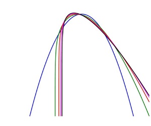
We finally compare the present results for this case with other previously proposed nonlinear distributions in figure 8. This figure specifically compares the data of Trulsen et al. (Reference Trulsen, Raustol, Jorde and Rye2020) and the present fifth-order PDF with (i) the third-order PDF of Longuet-Higgins (Reference Longuet-Higgins1963),
 \begin{equation} p(\zeta) =\frac{1}{\sqrt{2{\rm \pi}}}\exp\left(-\frac{\zeta^2}{2}\right) \left[1+\frac{\mathcal{S}}{6}\,H_3 + \left\{\frac{\mathcal{K}-3}{24}\,H_4+ \frac{\mathcal{S}^2}{72}H_6\right\} \right], \end{equation}
where
 $$\begin{gather} H_3 = \zeta^3 - 3\zeta, \end{gather}$$
 $$\begin{gather}H_4 = \zeta^4 - 6\zeta^2 + 3, \end{gather}$$
 $$\begin{gather}H_6 = \zeta^6 - 15\zeta^4 + 45\zeta^2 - 15, \end{gather}$$
and (ii) the second-order Tayfun (Reference Tayfun1980) distribution,
 \begin{equation} p(\zeta) = \frac{2}{{\rm \pi}\varepsilon}\int_{0}^\infty \left(\exp \left(- \frac{2x^2+2(1-C)^2}{\varepsilon^2} \right) + \exp \left(- \frac{2x^2+2(1+C)^2}{\varepsilon^2}\right)\right) \frac{\mathrm{d}\kern0.7pt x }{C}, \end{equation}
where
 \begin{equation} C = \sqrt{1+\varepsilon \zeta +x^2}. \end{equation}
Note that the Tayfun (Reference Tayfun1980) distribution assumes both narrow-bandedness of the spectrum as well as unidirectionality of the wave field. Note also that the integral in (6.7) is computed numerically, rather than utilizing e.g. the asymptotic approximation of Socquet-Juglard et al. (Reference Socquet-Juglard, Dysthe, Trulsen, Krogstad and Liu2005). Figure 8 clearly demonstrates that these previously proposed theoretical PDFs do not accurately describe the heavy positive tail inherent in this data set, which is again quite well predicted by the present fifth-order theory. It is emphasized that the present PDF requires only the relevant statistical moments (alternatively, the relevant cumulants) as input. Accurate reproduction of this challenging PDF has previously required detailed numerical simulations with fully nonlinear wave models; see e.g. figure 13(c) of Zhang & Benoit (Reference Zhang and Benoit2021).

Figure 8. Comparison of the PDF from the experiments of Trulsen et al. (Reference Trulsen, Raustol, Jorde and Rye2020) (circles with error bars) with the present fifth-order solution (solid line), the Tayfun (Reference Tayfun1980) second-order distribution (6.7) (red dashed line) and the Longuet-Higgins (Reference Longuet-Higgins1963, referred to as LH63) third-order distribution (6.5) (blue dotted line).
7. Conclusions
In this work, we have revisited the probability density function (PDF) for the free surface elevation in nonlinear irregular seas, based on the integral found originally by Longuet-Higgins (Reference Longuet-Higgins1963), stemming from the cumulant generating function. A new ordinary differential equation (ODE) has been derived, which governs this PDF to any desired order in nonlinearity, presented as (2.7). We emphasize that this ODE is free of any assumptions regarding narrow-bandedness of the spectrum or the directionality of the wave field. It has been confirmed that exact solutions of this ODE lead to the Gaussian distribution at first order, and the recently found Fuhrman et al. (Reference Fuhrman, Klahn and Zhai2023) distribution at second order.
Asymptotic solutions of this governing ODE have been derived analytically in the limit of large surface elevation, making use of the method of dominant balance. Up to a multiplicative constant, these provide the theoretical form of the positive tail of the PDF, thus newly clarifying how high-order cumulants (involving statistical moments such as the kurtosis, hyperskewness and hyperkurtosis) theoretically govern the positive tail. It is shown that the positive tail gets heavier at each successive order, implying increased probability of large surface elevations typical of rogue waves.
The asymptotic solutions have been utilized to generate boundary conditions, enabling backward numerical integration of the governing ODE. By ensuring a unit integral, this enables determination of the multiplicative constant, and hence the full theoretical PDF. The present work thus enables novel determination of the PDF to third order and above. Results up to fifth order have been derived explicitly, but the methodology can be extended trivially to any desired order in nonlinearity.
The new higher-order PDFs have been compared against those from data sets generated from irregular wave theory and fully nonlinear numerical simulations, as well as laboratory experiments. Focus has been exclusively on highly nonlinear cases in finite water depth, where second order is demonstrably inadequate. Generally excellent results have been found, even in the most challenging cases, confirming accuracy of the new high-order PDFs. In such highly nonlinear circumstances, the new PDFs have been shown to be far superior to previously existing theoretical methods.
Matlab and Python functions returning the new PDFs up to fifth order in nonlinearity are freely provided in the supplementary material. The authors sincerely hope that these may be useful for others wishing to utilize the new high-order PDFs in practice.
Supplementary material
Supplementary material for the present paper is available at https://doi.org/10.11583/DTU.24720564. This includes both Matlab and Python functions for computing PDFs (and tails) up to fifth order, as described in § 5. Additionally, the computed surface elevation data from § 6.2 are provided at https://doi.org/10.11583/DTU.25486948.
Funding
This research has been supported financially by the Independent Research Fund Denmark project STORM: STatistics and fOrces on stRuctures from extreMe water waves in finite depth (D.R.F. grant ID 10.46540/2035-00064B). This support is greatly appreciated.
Declaration of interests
The authors report no conflict of interest.


 Open access