


1. Introduction
The capability to predict high-Reynolds-number turbulent flows is essential for many natural and engineering flows such as external aerodynamics of wind turbines and aircraft wings, flow over the hull of marine vehicles, and atmospheric boundary-layer flow over complex landscapes and cityscapes, to name a few. However, due to extreme disparity of scales present in high-Reynolds-number wall-bounded turbulent flows, any attempt to simulate these flows directly on a computational grid without resorting to modelling of some sort results in prohibitively large computational cost. To resolve all the scales of the near-wall turbulent motions using direct numerical simulation (DNS), the required number of grid points scales as  $O(Re^{37/14})$, where $Re$ is the characteristic Reynolds number. Wall-resolved large-eddy simulation (WRLES), which resolves only the large (stress-carrying) eddies, reduces the grid point requirement to $O(Re^{13/7})$ (Choi & Moin Reference Choi and Moin2012). However, this level of computational cost is still unaffordable when the Reynolds number is high. As a cost-effective alternative to the above two approaches, wall-modelled large-eddy simulation (WMLES) resolves only the energetic eddies in the outer portion of the boundary layer, while the momentum transport within the unresolved near-wall region is accounted for by augmenting the wall-flux through a wall model. Thus, the no-slip condition at the wall is replaced by the Neumann boundary condition supplied by the wall model in the form of the wall shear stress. Note that the wall shear stress is computed by the wall model without ever resolving the near-wall scales. Therefore, the grid point requirement for WMLES reduces to $O(Re)$ (Choi & Moin Reference Choi and Moin2012), making the simulations of high-Reynolds-number flows feasible.
To date, several wall models have been proposed, most of which are based on some form of the law-of-the-wall or solving a set of simplified or full Reynolds-averaged Navier–Stokes (RANS) equations. Deardorff (Reference Deardorff1970) and Schumann (Reference Schumann1975) were the first to recognize the need for wall modelling to perform LES of high-Reynolds-number plane channels and annuli to overcome lack of computing resources in the 1970s. Grötzbach (Reference Grötzbach1987) later improved the model by removing the necessity of a priori knowledge of the mean wall shear stress. The geometry of the near-wall eddies was incorporated in the work of Piomelli et al. (Reference Piomelli, Ferziger, Moin and Kim1989) to account for the inclination of the vortical structures in the streamwise/wall-normal plane. Wang & Moin (Reference Wang and Moin2002) proposed an ordinary differential equation (ODE) based wall model derived from the equilibrium assumption (Degraaff & Eaton Reference Degraaff and Eaton2000), which later was extended to compressible flows (Bodart & Larsson Reference Bodart and Larsson2011; Kawai & Larsson Reference Kawai and Larsson2012). The ODE equilibrium wall model excludes the non-equilibrium effects such as pressure gradient, and considers the wall-normal diffusion only. Non-equilibrium wall models based on full three-dimensional (3-D) RANS equations were investigated by Balaras, Benoccis & Piomelli (Reference Balaras, Benoccis and Piomelli1996), Wang & Moin (Reference Wang and Moin2002), Cabot & Moin (Reference Cabot and Moin2000), Kawai & Larsson (Reference Kawai and Larsson2013) and Park & Moin (Reference Park and Moin2014, Reference Park and Moin2016a). Yang et al. (Reference Yang, Sadique, Mittal and Meneveau2015) introduced the integral non-equilibrium wall model based on the integrated boundary layer equations and assumed velocity profiles, which can be considered as a compromise between the aforementioned two classes of wall models. Similarly, Fowler, Zaki & Meneveau (Reference Fowler, Zaki and Meneveau2022) substituted the law-of-the-wall velocity profile into the wall normal integrated momentum balance and derived a Lagrangian relaxation towards an equilibrium transport equation for the friction-velocity vector. Several efforts have also been directed towards formulating wall models which are not based on RANS. Bose & Moin (Reference Bose and Moin2014) and Bae et al. (Reference Bae, Lozano-Durán, Bose and Moin2019) proposed a differential filter-based wall model which introduced a slip-velocity applied in the form of Robin boundary condition at the wall. Chung & Pullin (Reference Chung and Pullin2009) proposed a virtual wall model with a slip velocity boundary condition specified on the lifted virtual wall. Gao et al. (Reference Gao, Zhang, Cheng and Samtaney2019) extended this virtual wall model in a generalized curvilinear coordinate. Advances on WMLES were reviewed by Piomelli & Balaras (Reference Piomelli and Balaras2002), and more recently by Larsson et al. (Reference Larsson, Kawai, Bodart and Bermejo-Moreno2016) and Bose & Park (Reference Bose and Park2018). With the development of novel wall models and increase in the computing capacity, WMLES is becoming an indispensable tool for predictive but affordable scale-resolving simulation of practical engineering flows at high Reynolds numbers. Recent applications to external aerodynamics applications include simulation of a wing-body junction flow (Lozano-Durán, Bose & Moin Reference Lozano-Durán, Bose and Moin2022) and flow over a realistic aircraft model in landing configuration deploying high-lift devices (Goc et al. Reference Goc, Lehmkuhl, Park, Bose and Moin2021).
Although WMLES is now gaining popularity as a high-fidelity tool balancing the computational cost and the accuracy, with the potential to be used for design and optimization in practical engineering applications because of its reasonable turnaround times, comprehensive benchmark studies on the comparison of different wall models in complex flows are lacking. There have been a number of comparative studies of WMLES with different wall models or subgrid scale (SGS) models in canonical flows. For instance, Wang, Hu & Zheng (Reference Wang, Hu and Zheng2020) assessed the predictive capability of three wall models paired with four SGS models for the turbulence kinetic energy spectrum in the outer region in periodic channel flow to find out that the choice of SGS models (but not wall models) affect the result. Yang & Bose (Reference Yang and Bose2017) also conducted WMLES in periodic channel flow to provide a physics-based interpretation of the equivalence between the Robin-type wall closure (slip wall model) and the equilibrium wall model, along with comparison to the integral non-equilibrium wall model. Rezaeiravesh, Mukha & Liefvendahl (Reference Rezaeiravesh, Mukha and Liefvendahl2019) systematically studied the accuracy of WMLES using an algebraic wall model in predicting periodic channel flow, focusing on sensitivities to the choice of SGS models, matching height, grid resolution, and law of the wall parameters. It should be noted that the non-equilibrium terms that are added to the more complicated wall models are essentially inactive in canonical flows like a periodic channel flow. This fact limits the full understanding of the performance of wall models. Therefore, comparative studies of different wall models in more realistic turbulent flows with non-equilibrium effects, such as pressure gradient and mean-flow three-dimensionality, are highly desirable to understand the mechanism of certain wall models performing better than others, and to seek improvements of models based on such findings. Park (Reference Park2017) compared the performance of ODE equilibrium wall model and PDE non-equilibrium wall model in a separating and reattaching flow over the NASA wall-mounted hump. Kawai & Asada (Reference Kawai and Asada2013) investigated the capability of WMLES in transitional and separated flow over an airfoil near-stall condition with the equilibrium and non-equilibrium wall models. Lozano-Durán et al. (Reference Lozano-Durán, Giometto, Park and Moin2020) tested three RANS-based wall models (ODE equilibrium wall model, integral non-equilibrium wall model and PDE non-equilibrium wall model) in a three-dimensional transient channel flow. For the latter study, it is worth noting that the three wall models were not tested using the same LES code. The lack of a like-for-like comparison of different wall models, especially in flows with non-equilibrium effects such as mean-flow three-dimensionality and pressure gradient, warrants a systematic study of various wall models under the identical settings of the same solver and the same flow conditions. This will facilitate a clear assessment of the differences in the performance of different wall models, both in terms of accuracy and computational cost. Foregoing in view, in the present work, we test three wall models in a 3-D turbulent boundary layer (3DTBL) flow: an ODE equilibrium wall model (EQWM), an integral non-equilibrium wall model (integral NEQWM) and a PDE non-equilibrium wall model (PDE NEQWM). These three models respectively represent increasing model complexity with correspondingly increasing physical fidelity for predicting 3DTBL. The equilibrium wall model assumes that the velocity profile is unidirectional and neglects all non-equilibrium effects, while the latter two are capable of representing skewed velocity profiles and incorporate some or all non-equilibrium effects, albeit in an averaged sense.
Before describing the 3DTBL in more detail, a few remarks are in order regarding the suitability of the current choice of 3DTBL flow to conduct the comparative study of wall models with different physical fidelity. Historically, much of the research on wall turbulence has focused on statistically two-dimensional (2-D) equilibrium turbulence in simple geometries (e.g. channel, pipe and flat plate). Different wall models perform equally well therein, making it hard to justify the use of more complex models. Furthermore, many practical flows of interest, such as those found on the swept wings of aircraft, wing/body juncture, bow/stern regions of ships and turbomachinery, are strongly affected by the mean-flow three-dimensionality. Such 3DTBLs challenge the validity of the theories and models established from the canonical 2-D wall turbulence and thus provide a good stage to exhibit the distinctive capabilities of different wall models. Therefore, the current study of turbulent boundary layer with mean-flow three-dimensionality is well suited to test different wall models and to explain the physical origins of the differences in the results of these models.
The 3DTBLs can be classified as pressure-driven (also termed skew-induced (Bradshaw Reference Bradshaw1987) or inviscid-induced Lozano-Durán et al. Reference Lozano-Durán, Giometto, Park and Moin2020) or shear-driven (also termed viscous-induced Lozano-Durán et al. Reference Lozano-Durán, Giometto, Park and Moin2020) ones, according to the mechanisms by which the mean three-dimensionality is introduced into the flow. For the pressure-driven 3DTBLs, the cross-flow is induced by the imposition of spanwise pressure gradient. More specifically, the mean three-dimensionality is produced by reorienting (tilting) the existing mean spanwise vorticity to generate non-zero streamwise vorticity. This process is often referred to as ‘inviscid skewing’ due to its quasi-inviscid nature, and streamwise variation in the imposed spanwise pressure gradient often facilitates this vorticity tilting (Coleman, Kim & Spalart Reference Coleman, Kim and Spalart2000). Examples of this type of 3DTBLs include flows in a square duct with a bend (Flack & Johnston Reference Flack and Johnston1994; Schwarz & Bradshaw Reference Schwarz and Bradshaw1994), in an S-shaped duct (Bruns, Fernholz & Monkewitz Reference Bruns, Fernholz and Monkewitz1999), over wing-body junctures (Rumsey Reference Rumsey2018), over swept wings (Bradshaw & Pontikos Reference Bradshaw and Pontikos1985) and over prolate spheroids (Chesnakas & Simpson Reference Chesnakas and Simpson1994). For the shear-driven 3DTBLs, the cross-flow is induced by the viscous diffusion of mean spanwise shear from the wall. Examples of this class include flows within a spinning cylinder (Bissonnette & Mellor Reference Bissonnette and Mellor1974; Lohmann Reference Lohmann1976; Driver & Hebbar Reference Driver and Hebbar1989), over a rotating disk (Littell & Eaton Reference Littell and Eaton1993), over turbomachinery and in Ekman layers. In the present work, we are interested in the skew-induced cases which are more prevalent in external hydrodynamics or aerodynamics applications.
Over the past decades, studies on a 3DTBL have unravelled its distinctive features which set it apart from the canonical 2-D wall turbulence. First, the mean-flow direction in a 3DTBL varies along the wall-normal direction, resulting in a skewed velocity profile. The law-of-the-wall, which is the characteristic of the canonical 2-D wall turbulence, is therefore challenged in a 3DTBL. Second, the Reynolds shear stress vector is not aligned with the mean velocity gradient vector in 3DTBLs. Thus, the Reynolds shear stress response in a 3DTBL can lag behind or lead that predicted by the isotropic eddy viscosity models which assume perfect alignment of the two. Third, a reduction in the structure parameter (the ratio of the total Reynolds shear stress magnitude to twice the turbulent kinetic energy) is often observed in 3DTBLs, whereas this parameter is nearly constant (roughly 0.15) in the outer layer of a 2DTBL. The aforementioned features of a 3DTBL pose a fundamental challenge to the validity of the underlying assumptions in many turbulence models (including wall models) that are based on a 2DTBL, and therefore bring into question the reliability of these models when applied to practical flows.
The numerical studies of 3DTBLs using direct numerical simulation (DNS) and large-eddy simulation (LES) have mostly focused on deformed 2-D wall turbulence. These studies include channel flow subject to sudden cross-flow pressure gradients (Sendstad Reference Sendstad1992; Lozano-Durán et al. Reference Lozano-Durán, Giometto, Park and Moin2020), channel flow with spanwise wall motions, channel flow subject to mean strains (Coleman et al. Reference Coleman, Kim and Spalart2000), a TBL over an idealized infinite swept wing generated by a transpiration profile (Coleman, Rumsey & Spalart Reference Coleman, Rumsey and Spalart2019), a TBL subject to streamwise-varying pressure gradient (Bentaleb & Leschziner Reference Bentaleb and Leschziner2013) and a TBL on a flat plate with a time-dependent freestream velocity vector (Spalart Reference Spalart1989). These numerical studies are limited to relatively low Reynolds number and idealized 3DTBLs due to the large computational cost. The present study focuses on a realistic, spatially developing, pressure-driven 3DTBL over the floor of a duct with a bend (Schwarz & Bradshaw Reference Schwarz and Bradshaw1994), which is at a considerably higher Reynolds number than the past studies but still provides a good balance between the physical realism, the tractability of the underlying 3DTBL mechanisms, and the computational cost of the simulations.
The major objectives of this work is to systematically compare wall models in a skew-induced 3DTBL and to provide a physics-based explanation of their differing performances. We consider the three aforementioned wall models that potentially span the complete spectrum of the available RANS-based wall models with varying physical details and complexity. A fully 3-D flow with no homogeneous direction is considered for this purpose. Another objective is to understand the characteristics of the skew-induced 3DTBL, especially compared with the viscous-induced 3DTBL. The paper is organised as follows. The computational details including the flow configuration, boundary conditions and wall-model formulations are discussed in § 2. The flow statistics obtained from WMLES are presented in § 3. Based on these results, the performance of different wall models are compared and the characteristics of this pressure-driven 3DTBL are discussed based on the anisotropy invariant map and the Johnston triangular plot. The effects of different non-equilibrium terms in wall models in terms of predicting near-wall flow direction are also quantified. Finally, conclusions are given in § 4.
2. Computational details
2.1. Flow configuration
The reference configuration for the present study is the experimental set-up of Schwarz & Bradshaw (Reference Schwarz and Bradshaw1994). While numerous experimental studies have been reported on 3DTBLs (as discussed in Johnston & Flack Reference Johnston and Flack1996), our choice of the reference experiment was motivated primarily by the following aspects of Schwarz & Bradshaw (Reference Schwarz and Bradshaw1994) which we found to be favourable to the goals of this study: (1) the highest Reynolds number among the pressure-driven 3DTBLs experiments reported by Johnston & Flack (Reference Johnston and Flack1996); (2) availability of the mean velocity and full Reynolds stress profiles; and of (3) the skin friction (magnitude and orientation) and pressure distribution along the wall. However, some remarks are also in order regarding limitations of the experiment. First, direct wall-stress data are not available, instead, a fit to the log law near  $y^+ \approx 100$ was used for indirect stress measurement. Second, the description of the zero-pressure gradient region far upstream of the bend region for the purpose of computational fluid dynamics (CFD) inflow generation is incomplete, therefore requiring an iterative procedure in the inflow generation to match the reported statistics at the first streamwise measurement station.
The experiment featured a spatially developing incompressible turbulent boundary layer, growing along the floor of a square duct with a 30 $^{\circ }$ bend (see figure 1). It should be noted that the boundary layer on the floor was very thin compared to the duct height, with $\delta _{99}/D$ ranging between 0.026 and 0.07 throughout the test section, where $D$ is the width (or height) of the square duct. The flow was far from being fully developed, and the secondary flow near the corner regions was expected to have negligible influence on the centreline region, which was the primary region of interest in the experiment.

Figure 1. Schematic of the floor of the duct (reproduction from figure 1 of Schwarz & Bradshaw Reference Schwarz and Bradshaw1994). The measurement locations in the experiment are marked as numbers 0–21 along the duct centreline. Two coordinate systems are employed. Here,  $(x,y,z)$ is a fixed coordinate system with the origin located at the inlet and $(x',y',z')$ is a curvilinear coordinate system aligned with the local duct centreline (measurements in mm).
Following Schwarz & Bradshaw (Reference Schwarz and Bradshaw1994), two coordinate systems are employed here to facilitate the presentation of the results:  $(x,y,z)$ denotes the global Cartesian coordinate system; $(x',y',z')$ denotes a curvilinear coordinate system aligned with the local duct centreline. Here, $y = y'$ are the wall-normal coordinates (distance from the floor of the duct). In the experiment, the boundary layer on the floor was tripped using a trip wire at the duct inlet located at $x'=0$, thus ensuring a turbulent boundary layer over the entire floor of the test section. Boundary layers on the other three walls of the duct were not tripped (Schwarz, private communication, 2019). The Reynolds number was moderately high, with $Re_{\theta }$ ranging between 4100 and 8500 (or $Re_{\tau }$ roughly ranging between 1500 and 3900). The flow along the centreline upstream of the bend was reported to exhibit typical characteristics of the canonical 2-D zero pressure gradient (ZPG) flat-plate boundary layer. Mean-flow three-dimensionality was generated in the bend region approximately between $x'=1626$ mm and $x'=2224$ mm due to the cross-stream pressure gradient induced by the bend. The surface streamlines were deflected by up to $22^{\circ }$ relative to the local duct centreline. Downstream of the bend, the 3DTBL gradually returned to a 2DTBL owing to the vanished spanwise pressure gradient. The experimental study focused on the boundary layer along the local centreline where the streamwise pressure gradient was found to be small.
The computational domain is identical to the test section in the experiment, which consisted of a square duct ( $D\times D= 0.762\ {\rm m} \times 0.762\ {\rm m}$) with a total curved length of $L = 3.748$ m, as shown in figure 1. Two grid resolutions are considered in the present study: a coarse mesh with 8 million control volumes and a fine mesh with 38 million control volumes. Figure 2 shows the near-wall grid spacing distributions along the duct centreline in the two meshes. The computational meshes are designed to maintain adequate wall-modelled LES grid resolution in the test section such that the local boundary layer contains approximately 16–23 and 32–45 cells across its thickness in the coarse and fine computational meshes, respectively. Local grid adaptations were applied in the near-wall region with the effect that the grid resolution transitions from the coarser isotropic-cell region in the free stream ( $\varDelta = 0.008$ m at $y/D > 0.1$) towards the finer near-wall region on the duct floor through anisotropic grid refinements. This resulted in wall-parallel grid resolutions ( ${\rm \Delta} x = {\rm \Delta} z$) of 4 and 2 mm for the coarse and fine meshes, respectively. In the region upstream of the bend ( $x'/L \le 0.43$) where the boundary layer was thin but grew fast, the wall-normal grid spacings were varied with $x'$ to keep the number of boundary-layer-resolving cells approximately constant, resulting in ${\rm \Delta} y = 0.86\ {\rm mm} \sim 2.2\ {\rm mm}$ and ${\rm \Delta} {y} = 0.43\ {\rm mm} \sim 1.1\ {\rm mm}$ for the coarse and fine meshes, respectively. At $x'/L \ge 0.43$, ${\rm \Delta} y$ was fixed at their maximum values aforementioned. Compared to Cho et al. (Reference Cho, Lozano-Durán, Moin and Park2021) where WMLES of the same geometry using isotropic voronoi cells was reported, the present study using anisotropic hexahedral cells deploys roughly the same wall-normal resolutions and approximately twice coarser wall-parallel resolutions in and downstream of the bend. Total cell counts are significantly reduced as a result, while maintaining higher numbers of cells across the thickness of the local boundary layer. The grid-resolution transition zones are located sufficiently away from the shear layer on the duct floor, so that the solution therein is not affected by the accuracy degradation associated with abrupt changes in grid resolution.

Figure 2. (a) Near-wall grid spacing distributions in wall units (based on the local skin friction) along the duct centreline. (b) Near-wall grid spacing distributions (normalized by duct height  $D$) along the duct centreline. Solid lines, wall-parallel grid spacing ( ${\rm \Delta} x = {\rm \Delta} z$); dashed lines, wall-normal grid spacing ( ${\rm \Delta} y$). Black, coarse mesh; blue, fine mesh.
2.2. Inflow characterization and boundary conditions
Setting the appropriate boundary conditions in the simulation, particularly for the reproduction of flow characteristics upstream of the bend region where a typical equilibrium 2DTBL is expected, is crucial before attempting to compare the simulation results with the experimental results at any downstream location. However, the experiment reports flow statistics at the 22 locations shown in figure 1 along the duct centreline, with the first measurement location being far downstream of the test section inlet (at  $x'=826$ mm). In the absence of this critical flow information at $x'=0$ mm, where the boundary layer on the floor was tripped in the experiment, we resort to a synthetic turbulence generation based on a digital filter approach (Klein, Sadiki & Janicka Reference Klein, Sadiki and Janicka2003) for approximating the inflow boundary condition, rather than trying to replicate the trip-wire transition in the experiment. This approach requires iterative guesses on the length of the development region (if any) to be appended upstream of the nominal trip location in the experiment ( $x'=0$ mm), and the state of the inflow to be prescribed at the new inlet location. It should be noted that the goal here is to reproduce the 2DTBL upstream of the bend reasonably well, which then acts as the inflow for the 3DTBL within the bend, rather than to exactly match the flow conditions at the test section inlet. After iterating on several inflow conditions and the inlet location, we found that prescribing a flat-plate turbulent boundary layer at $Re_{\theta }=2560$ (Schlatter et al. Reference Schlatter, Li, Brethouwer, Johansson and Henningson2010) at the nominal inlet ( $x'=0$ mm) reproduces the boundary layer statistics well at the first measurement location (station 0: $x'=826$ mm). As shown in figure 3, the simulation agrees well with the experiment in terms of the distributions of the boundary layer and momentum thicknesses. In figure 4, it is observed that the profiles of the mean velocity and Reynolds stress components from the present calculation agree well with the experiment at the first measurement station (station 0: $x'=826$ mm), as well as with a WRLES of a zero pressure gradient flat-plate boundary layer (ZPGFPBL) at a comparable Reynolds number ( $Re_\theta = 4100$, Schlatter et al. Reference Schlatter, Li, Brethouwer, Johansson and Henningson2010).

Figure 3. Centreline distributions of (a) boundary layer thickness and (b) momentum thickness (coarse mesh). Symbols, experiment; red dash–dotted line, equilibrium wall model; blue solid line, PDE non-equilibrium wall model; green dashed line, integral non-equilibrium wall model. Black vertical dashed lines denote the start and end of the bend region.

Figure 4. (a) Mean velocity profile at the first measurement station in the experiment (station 0:  $x'= 826$ mm). Black squares are from the experiment. Black dots, WRLES by Schlatter et al. (Reference Schlatter, Li, Brethouwer, Johansson and Henningson2010) at the same Reynolds number ( $Re_{\theta } = 4100$); red, equilibrium wall model; blue, PDE non-equilibrium wall model; green, integral non-equilibrium wall model (solid lines represent coarse mesh results; dashed lines represent fine mesh results). Black dashed lines denote the law of the wall (viscous sublayer: $u^+ = y^+$; log-law: $u^+ = \frac {1}{0.41}\log y^++5.2$). (b) Reynolds stress profiles at the first measurement location (station 0: $x'=826$ mm). Big symbols are from the experiment: circles, $\overline {u'u'}$; stars, $\overline {v'v'}$; triangles, $\overline {w'w'}$; squares, $\overline {u'v'}$. Different lines and dots have the same denotations as in panel (a).
The prescription of boundary conditions on the rest of the boundaries is relatively straightforward. A subsonic Navier–Stokes characteristic boundary condition (Poinsot & Lele Reference Poinsot and Lele1992) is imposed at the outlet of the duct. No attempt was made to resolve the boundary layers on the two side walls and the top wall which were not tripped in the experiment. The no-slip boundary condition is applied to each of these walls. The wall model is applied to the bottom wall, and the wall stress calculated from the wall-model solution is used as the Neumann boundary condition on this wall. All walls are assumed to be thermally adiabatic.
The computational time step was fixed at  $U_\infty {\rm \Delta} t / D = 2.2 \times 10^{-4}$ in all calculations with the coarse mesh. All simulations were initialized with a uniform flow everywhere in the domain. After ten flow-through times ( $L/U_{\infty }$), the flow was observed to be free from the initial transient and deemed fully developed. After this initial transient, the flow statistics were accumulated over additional ten flow-through times.
2.3. Flow solver and subgrid scale (SGS) / near-wall modelling
The simulations were performed with CharLES, an unstructured cell-centred finite-volume compressible LES solver developed at Cascade Technologies, Inc. The solver employs an explicit third-order Runge–Kutta (RK3) scheme for time advancement and a second-order central scheme for spatial discretization. More details regarding the flow solver have been reported by Khalighi et al. (Reference Khalighi, Nichols, Ham, Lele and Moin2011) and Park & Moin (Reference Park and Moin2016a). The Vreman model (Vreman Reference Vreman2004) is used to close the SGS stress and heat flux. In Appendix A, the effect of SGS stress models is discussed along with the results obtained with the dynamic Smagorinsky model and dynamic tensor-coefficient Smagorinsky model (Moin et al. Reference Moin, Squires, Cabot and Lee1991; Lilly Reference Lilly1992; Agrawal et al. Reference Agrawal, Whitmore, Griffin, Bose and Moin2022).
In WMLES, LES equations are solved on a coarse mesh, where the stress-carrying eddies in the near-wall region are mostly unresolved. The LES mesh alone cannot represent the sharp velocity gradients and the momentum transport near the wall. This causes SGS models to produce insufficient levels of modelled stresses. Wall modelling aims to compensate for such numerical and modelling errors in the underresolved near-wall region of LES, by augmenting the total stresses directly through the imposition of the modelled stress boundary condition at the wall in lieu of the no-slip condition. In the present work, wall models solve simplified, vertically integrated or full RANS equations on a separate near-wall mesh. The grid for wall models have fine resolution in the wall-normal direction (with the exception of the integral non-equilibrium wall model, which does not require a wall-normal grid), but the wall-parallel grid resolution (if any) is identical to or coarser than the LES grid. All wall models in this study are driven by the LES states imposed at their top boundaries, which are taken at a specified matching height in the LES grid. At each time step, wall stress and heat flux obtained from the wall model are used as the Neumann wall boundary condition for the LES. Figure 5 shows a schematic of the wall modelled LES procedure employed in the present work.

Figure 5. Sketch of the wall-modelling procedure (reproduction from figure 1 of Park & Moin Reference Park and Moin2016a). Wall shear stress ( $\tau _w$) and heat flux ( $q_w$) are solved from the wall model equations on a separate near-wall mesh. Wall models are driven by the LES states imposed at their top boundaries while the no-slip condition is applied at the wall.
In the present work, the location at which the wall-models take input from the LES (matching height, denoted as  $h_{wm}(x)$) is fixed across different grid resolutions by setting it to the centroids of the third off-wall cells or the top faces of the fifth off-wall cells in the coarse and fine meshes, respectively, corresponding to $10^3 h_{wm} / D = 3 \sim 7$ or $h^+_{wm} = 175 \sim 375$ in inner units. This has the effect of fixing the wall-modelled regions in LES during grid refinements, so that improvement in LES prediction is not associated with the change in wall-modelling details, but it is attributed largely to the grid adaptation. This choice is also motivated by our experience with the flow solver, where restricting $h_{wm}$ to the first off-wall cell or in the buffer layer produced non-trivial log-layer mismatch in channel flow calculations, even with the filtration of the wall-model input as suggested by Yang, Park & Moin (Reference Yang, Park and Moin2017) for a structured pseudospectral/finite-difference code. Owen et al. (Reference Owen, Chrysokentis, Avila, Mira, Houzeaux, Borrell, Cajas and Lehmkuhl2020a) reported a similar need for using the LES velocity further away from the wall in their finite-element-based WMLES of channel and wall-mounted hump. Readers are referred to Appendix B, where additional accounts on the matching height are provided along with numerical experiments to examine the effect of varying matching height on the prediction of mean three-dimensionality.
The three wall models considered in the present study are an equilibrium stress model (EQWM) in the form of ordinary differential equations, an integral non-equilibrium wall model (integral NEQWM) that solves the vertically integrated Navier–Stokes equations and a PDE non-equilibrium wall model (PDE NEQWM) that retains the complexity of the full Navier–Stokes equations. All three wall models parametrize the unresolved turbulence in the wall-model domain in a statistical sense using simple RANS models based on the mixing-length formulation. Note that the EQWM and PDE NEQWM have previously been implemented in CharLES, and they have been tested extensively through various studies (Bodart & Larsson Reference Bodart and Larsson2012; Park & Moin Reference Park and Moin2014, Reference Park and Moin2016a,Reference Park and Moinb; Park Reference Park2017). The integral NEQWM was recently integrated into CharLES, the implementation aspects of which will be discussed in a future article (Hayat & Park Reference Hayat and Park2021). A brief description of each of these models is given below.
The EQWM (Bodart & Larsson Reference Bodart and Larsson2011; Kawai & Larsson Reference Kawai and Larsson2012) solves the simplified boundary layer equations which account only for the wall-normal diffusion:
 $$\begin{gather} \frac{{\rm d}}{{\rm d} \eta}\left[(\mu + \mu_{t})\frac{{\rm d} u_{||}}{{\rm d} \eta}\right] = 0, \end{gather}$$
 $$\begin{gather}\frac{{\rm d}}{{\rm d} \eta}\left[(\mu + \mu_{t})u_{||}\frac{{\rm d} u_{||}}{{\rm d} \eta}+(\lambda + \lambda_{t})\frac{{\rm d}T}{{\rm d} \eta}\right] = 0, \end{gather}$$
where  $\eta$ is the local wall-normal coordinate, $u_{||}$ is the wall-parallel velocity magnitude, $T$ is the temperature, $\mu$ is the molecular viscosity, $\lambda$ is the molecular thermal conductivity, and $\mu _t$ and $\lambda _t$ are the turbulent eddy viscosity and conductivity, respectively. It should be note that Ma = 0.2 in the simulations (the Mach number was not reported in the experiment as the authors of the experiment clearly assumed the flow was incompressible). Although the energy equation is solved, variations of thermodynamic variables are very small, and the energy equation does not play an important role in the present study. The velocity vector is assumed to be aligned with the LES velocity at the matching height. Owing to this intrinsic assumption, the equilibrium wall model is incapable of predicting skewed velocity profiles within the wall-modelled domain. Also, due to the unidirectionality and the condition $\mu +\mu _t > 0$, the EQWM can represent monotonic velocity profiles only, and it cannot predict velocity profiles with sign changes in the slope as found in the near-wall regions of separated shear layers. The wall-model eddy viscosity $\mu _t$ is based on the following mixing-length formula:
 \begin{equation} \mu_{t} = \kappa \rho y\sqrt{\frac{\tau_w}{\rho}}D,\quad D=[1-{\rm exp}(-y^+{/}A^+)]^2. \end{equation}
However, the PDE NEQWM (Park & Moin Reference Park and Moin2014, Reference Park and Moin2016a) solves the full 3-D unsteady RANS equations:
 $$\begin{gather} \frac{\partial \rho}{\partial t} + \frac{\partial \rho u_{j}}{\partial x_{j}}=0, \end{gather}$$
 $$\begin{gather}\frac{\partial \rho u_{i}}{\partial t} + \frac{\partial \rho u_{i}u_{j}}{\partial x_{j}} + \frac{\partial p}{\partial x_{i}}=\frac{\partial \tau_{ij}}{\partial x_{j}}, \end{gather}$$
 $$\begin{gather}\frac{\partial \rho E}{\partial t} + \frac{\partial(\rho E+p)u_{j}}{\partial x_{j}}=\frac{\partial \tau_{ij}u_{i}}{\partial x_{j}}-\frac{\partial q_{j}}{\partial x_{j}}, \end{gather}$$
where  $\rho$ is the density and $u_{i}$ is the velocity component, $p$ is pressure and $E=p/[\rho (\gamma -1)]+u_{k}u_{k}/2$ is the total energy. The stress tensor and heat flux are given by $\tau _{ij}=2(\mu +\mu _t){\mathsf{S}}_{ij}^d$ and $q_{j}=-(\lambda + \lambda _{t})({\partial T}/{\partial x_{j}})$. For the RANS closure, a novel mixing-length model is used, which dynamically accounts for the resolved Reynolds stresses carried by the wall model (Park & Moin Reference Park and Moin2014). The wall-model mesh for the PDE NEQWM has the same wall-parallel grid content as in the coarse LES mesh, but it is refined in the wall-normal direction to resolve the viscous sublayer.
Lastly, the integral NEQWM formulation solves a similar set of equations as the PDE NEQWM, albeit in a wall-normal integrated form. Currently, this formulation is limited to incompressible flows, and therefore the energy equation is not solved. For the sake of brevity, only the 2-D formulation (the wall-normal and one wall-parallel velocity components) is presented below, and the reader is referred to Yang et al. (Reference Yang, Sadique, Mittal and Meneveau2015) for the details of full 3-D formulation. The vertically integrated momentum equation is given by
 \begin{align} \frac{\partial}{\partial t}\int_{0}^{h_{wm}} u\, {{\rm d} y} + \frac{\partial }{\partial x} \int_{0}^{h_{wm}} u^2\, {{\rm d} y} - U_{LES} \frac{\partial}{\partial x} \int_{0}^{h_{wm}} u\, {{\rm d} y} = \frac{1}{\rho} \left[-\frac{\partial p}{\partial x} h_{wm} +\tau_{h_{wm}} - \tau_{w}\right], \end{align}
where  $x$ and $y$ represent the local wall-parallel and wall-normal coordinates, $h_{wm}$ is the matching height, $U_{LES}$ is the time-filtered velocity from the LES solution at the matching location. Here, $\tau _{w} = \mu ({\partial u}/{\partial y})|_{y=0}$ and $\tau _{h_{wm}} = (\mu +\mu _{t})({\partial u}/{\partial y})|_{y=h_{wm}}$ are the shear stresses at the wall and at the matching location, respectively. The integral terms are evaluated by assuming an analytical composite profile for the velocity within the wall model, which has the form:
 $$\begin{gather} u = u_{\tau} \frac{y}{\delta_{\nu}} = \frac{u_{\tau}^2}{\nu}y, \quad 0 \leq y \leq \delta_{i}, \end{gather}$$
 $$\begin{gather}u = u_{\tau}\left[\frac{1}{\kappa} \log \frac{y}{h_{wm}}+C\right]+u_{\tau} A \frac{y}{h_{wm}}, \quad \delta_{i}< y \leq h_{wm}, \end{gather}$$
where the unknown parameters  $A$,
$A$,  $C$,
$C$,  $u_{\tau }$ and $\delta _{i}$ are determined from the solution of (2.7) along with suitable matching and boundary conditions. For the full 3-D formulation consisting of two wall-parallel velocity components, like that employed for the present study, the composite profiles have a total of 11 unknown parameters. This approach attempts to model the effects of pressure gradient and advection through the last term in (2.9) representing linear departure from the log law.
It is worth mentioning here that in the original 3-D formulation of Yang et al. (Reference Yang, Sadique, Mittal and Meneveau2015), the assumed form of the viscous-sublayer velocity profiles in the two wall-parallel directions ((C5) in Yang et al. Reference Yang, Sadique, Mittal and Meneveau2015) resulted in inconsistent asymptotic behaviour of velocity near the wall. This made the wall-stress predictions of the wall model highly sensitive to the choice of the local  $x/z$ coordinate axes. In our current integral NEQWM formulation, we modify the assumed viscous-sublayer profile to ensure consistent near-wall asymptotic behaviour as given by the Taylor series expansion. The modified formulation is briefly described in Appendix C, and its details along with its implementation in an unstructured solver are presented by Hayat & Park (Reference Hayat and Park2021). A MATLAB implementation for the EQWM and the modified integral NEQWM is available on GitHub at https://github.com/imranhayat29/Wall-Models-for-LES.
A remark is in order regarding the overall cost of simulations with different wall models. The computational costs of the three wall models were compared by running the simulations on the fine LES mesh with 256 CPU cores for three convective flow-through times. When the cost of the simulation without any wall model (no-slip LES) is taken as the unity, the simulation costs are 1.27, 1.2 and 2.2 with the EQWM, the integral NEQWM and the PDE NEQWM, respectively. The higher cost with the PDE NEQWM is due to the inversion of a large linear system required as a part of implicit time advancement.
3. Results
Results from the WMLES simulations are discussed in this section. Overall characteristics of the flow are first highlighted from the instantaneous flow field standpoint. Mean and turbulence statistics obtained with different wall models are then assessed against the experimental data. Furthermore, the three-dimensionality of the outer portion of the boundary layer is examined with the aid of Reynolds stress anisotropy and the Johnston triangular plot.
Some remarks are in order concerning the ways in which the main results are presented in this paper. The primary interest of the experiment was to examine the effect of the mean three-dimensionality in the absence of strong streamwise pressure gradient. To this end, the experiment presented the key flow statistics along the floor centreline, where the axial pressure gradient was observed to be nearly zero. It should be noted, however, that the mean-flow trajectory near the wall deviates somewhat substantially from the centreline as the flow passes through the bend region, as observed from the instantaneous flow field (figure 7) and the near-wall streamlines (figure 10b). This leaves some ambiguity in the interpretation of the statistics presented along the centreline, because any two fluid particles on the centreline (in and after the bend region) would have travelled along different Lagrangian trajectories, experiencing different history effects (most notably, they are subject to different upstream axial/spanwise pressure gradients). With this limitation in mind, we still choose to show our results along the centreline, as all experimental data (except the wall-pressure) were presented as so.
3.1. Grid convergence
Figure 6 shows the mean-flow statistics and the Reynolds stresses at  $x'=1875$ mm (the eighth measurement station in figure 1), as well as the centreline skin-friction coefficient $C_{f}$ distribution obtained from the EQWM LES with the coarse and the fine grids described in § 2.1. The skin-friction coefficient is defined as
 \begin{equation} C_{f}=\frac{\tau_{w}}{\frac{1}{2}\rho U^2_{e}}, \quad \frac{U_e}{U_{ref}}=(1-C_{p})^{1/2}, \end{equation}
where  $\tau _w = \sqrt {\tau _{w,x}^2+\tau _{w,z}^2}$ is the magnitude of the mean wall shear stress vector and $U_e$ is the local free stream velocity. The pressure coefficient is defined as
 \begin{equation} C_{p} = \frac{p-p_{ref}}{\frac{1}{2}\rho U^2_{ref}}. \end{equation}
Following the experiment,  $p_{ref}$ is the static pressure at $x'=0$ mm and $U_{ref}$ is the free stream velocity at $x'=826$ mm (defined at the spanwise centreline). Although only the EQWM results are shown here for brevity, it is noted that the other two wall models exhibited similar grid-convergence characteristics. In figure 6(a), both the mean velocity and the mean-flow direction (defined by the angle between the mean velocity vector and the free stream velocity vector) profiles obtained from the coarse-grid calculation are already in good agreement with the experiment, and the results only improve marginally with the grid refinement. More importantly, this points towards the grid convergence of the results for the refinement level used in this study. Figure 6(b) shows the skin-friction distribution along the centreline of the duct. Between the first and the last measurement stations, we observe a reasonably converged $C_{f}$, with the fine-grid calculation producing slight improvement in $C_{f}$. In figure 6(c), a similar trend is observed for all the Reynolds stress components shown, with the exception of the streamwise component of the Reynolds normal stress, which shows noticeable variation with grid refinement in the near-wall region; however, the Reynolds stresses in the outer portion of the boundary layer have largely converged. Having established reasonable evidence of grid-convergence for most of the flow statistics on the coarse grid, the remainder of this paper will focus largely on discussing the results obtained with the coarse grid unless stated otherwise.

Figure 6. Grid convergence of the EQWM LES. (a) Blue, mean-flow direction versus distance from the wall; red, mean velocity magnitude profile. (b) Centreline distribution of the skin-friction coefficient and (c) Reynolds-stress profiles. Red,  $\overline {u'u'}$; blue, $-\overline {u'v'}$; green, $\overline {v'w'}$. Solid lines, coarse grid; dashed line, fine grid. Profiles in panels (a) and (c) are at $x'=1875$ mm (station 8). Black vertical dashed lines in panel (b) denote the start and end of the bend region.
3.2. Instantaneous flow field
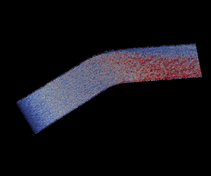
Figure 7 visualizes the vortical structures in the floor boundary layer. Near the inlet (approximately within 20 times the inlet boundary-layer thickness from the inlet), structures with less coherence resulting from the synthetic inflow turbulence generation are observed. The floor boundary layer then gradually develops into a coherent fully developed state far upstream of the bend region, which is also verified by the velocity profile at  $x'=826$ mm (figure 4) following the typical law of the wall observed in a 2-D turbulent boundary layer. When the flow enters the bend region, a clear contrast of two boundary layers with different origins (blue and red regions) are observed. The boundary layer in the red region is thicker than that in the blue region, showing that a new boundary layer is emerging from the concave sidewall within the bend region (at $z<0$) and the original boundary layer developed from the upstream section is turning rapidly towards the convex side (at $z>0$). This overall flow behaviour is visually in fair agreement with the surface oil visualization in the experiment as shown in the inset in figure 7.

Figure 7. Visualization of the near-wall vortical structures using the isosurfaces of  $Q$ (
$Q$ ( $Q = Q_{rms}$, where $Q$ is the second invariant of the velocity gradient tensor), coloured by the distance from the floor of the duct. Flow is from the bottom left to the top right. Surface oil visualization from the experiment (Schwarz & Bradshaw Reference Schwarz and Bradshaw1994) is shown in the inset (figure reprinted with permission from Schwarz & Bradshaw (Reference Schwarz and Bradshaw1994).
3.3. Mean-flow statistics
The cross-stream pressure gradient is the source of the mean three-dimensionality in the bend region. It acts to deflect the streamlines close to the wall more strongly than those near the free stream. It is therefore important to first establish close agreement in the pressure distribution close to the bend between the simulation and the experiment. Note that in the current case without flow separation, the pressure distribution is determined largely by the wall geometry and the inviscid effect, presumably unaffected by the wall-modelling details. Figure 8 shows the distribution of the static wall-pressure coefficient on the floor of the duct. The wall-pressure probing lines are parallel to the duct centreline, as shown in the inset figure. The figure shows good agreement between the simulation and the experiment, except in the recovery region downstream of the bend. The axial pressure gradient is almost zero along the centreline. However, a significant spanwise pressure gradient starts to develop upstream of the bend, reaches a maximum within the bend region and eventually decays to zero downstream of the bend. The reason for disagreement in the recovery region remains unclear to us. While  $C_p$ in the experiment remains to be slightly negative near the outlet, $C_p$ in the simulation naturally vanishes to its upstream zero value as the flow relaxes back to its 2-D ZPG state. Note that the experiment reported only the centreline distribution in this region and that extending the duct further downstream in the simulation did not change the trend.

Figure 8. Variation of the wall-pressure coefficient from coarse EQWM simulation (results from the other wall models and resolutions are almost identical). Symbols are from the experiment. Colours denote different spanwise locations corresponding to the inset figure. Here,  $z':0$ mm, ${\pm }127$ mm, ${\pm }254$ mm, ${\pm }368$ mm.
Figure 9 shows the distribution of the skin-friction coefficient along the duct centreline. The centreline mean-flow is expected to agree well with the canonical ZPG 2DTBL in this region. A deviation of the skin friction from the ZPG 2DTBL near the inlet is the artefact of the inflow treatment. Note that the synthetic inflow turbulence generation methods when applied to DNS or wall-resolved LES of low Reynolds number are known to produce a development length of 10–20 initial boundary layer thicknesses ( $\delta _{in}$), through which coherence-lacking artificial structures mature into fully developed turbulence (e.g. Patterson, Balin & Jansen (Reference Patterson, Balin and Jansen2021), Sandberg (Reference Sandberg2012), Larsson (Reference Larsson2021) where $Re_\tau = 400 \sim 500$). The present high-Reynolds-number case simulated with very coarse meshes produced longer development lengths ( $30\unicode{x2013}40 \delta _{in}$). The flow was observed to be fully developed from slightly upstream of the first measurement station, after which the WMLES results are in reasonable agreement with the experiment as well as with an empirical correlation (Fernholz & Finley Reference Fernholz and Finley1996) and a wall-resolved LES of ZPG 2DTBL (Eitel-Amor, Orlu & Schlatter Reference Eitel-Amor, Orlu and Schlatter2014). In figure 9(b), slight overprediction of the skin friction from WMLES is observed throughout the duct. A similar trend was reported by Cho et al. (Reference Cho, Lozano-Durán, Moin and Park2021), where the EQWM was used with up to 76 million control volumes in LES. It should be noted that the wall shear stresses were measured indirectly in the experiment using a Preston tube and Patel's calibration (Patel Reference Patel1965) for a 2DTBL. Patel (Reference Patel1965) reported that errors as large as 6 % could occur when a Preston tube is used in flows with moderate streamwise pressure gradient. Next, we examine the mean three-dimensionality of the flow in the duct. The variation of the surface flow direction relative to the free stream direction is a measure of the mean-flow three-dimensionality. As shown in figure 10(a), the cross-flow is almost zero in the upstream and it grows rapidly as the flow approaches the bend. The resulting turning angle reaches the maximum near the end of the bend and decays gradually thereafter. These observations are consistent with the development of the spanwise pressure gradient. All three wall models predict the general trend in the turning-angle variation correctly; however, the PDE NEQWM gives the most accurate prediction among the three (especially within the bend region), followed by the integral NEQWM and then the EQWM. The maximum difference between the PDE NEQWM and the EQWM is roughly $5^{\circ }$ occurring at $x'/L=0.49$ within the bend. Note that the total flow turning is an accumulative effect of the local flow change, and the area under the curve in figure 10(a) can be thought of as an approximation of the near-wall total flow turning angle. Related to this, figure 10(b) visually highlights predictions of the near-wall flow direction by different wall models in terms of the select surface streamlines calculated from the mean wall shear-stress vector. It can be clearly seen that the flow deviates from the local centreline; however, the deviation is not predicted evenly across the different wall models, consistent with our observation in the flow turning angles in figure 10(a). The surface flow from the PDE NEQWM turns much more rapidly than that from the EQWM. In figure 11, profiles of the mean-velocity magnitude are compared between the different wall models and the experiment, at several locations along the centreline, including upstream of, within and downstream of the bend. It can be seen that the no-slip LES, which does not employ a wall model, gives a very poor prediction of the mean velocity. Here, a higher momentum is imparted to the boundary layer as a consequence of the underpredicted wall shear force. With the introduction of wall modelling, a significant improvement is achieved in the predicted mean-velocity profiles. In line with the predictions of the skin-friction coefficient in figure 9, the mean velocity profiles across the three wall models are almost identical. Note that here, the profiles only show the magnitude of the mean velocity, thus lacking information on the three-dimensionality of the mean flow.

Figure 9. Centreline distribution of the skin-friction coefficient ( $C_f$). (a) $C_f$ versus $Re_{\theta }$ upstream of the bend. (b) $C_f$ versus axial location. Squares, experiment; red dash–dotted line, EQWM; blue solid line, PDE NEQWM; green dashed line, integral NEQWM. In panel (a): black dotted line, ZPGFPBL empirical correlation ((9) in Fernholz & Finley Reference Fernholz and Finley1996); black dashed line, WRLES of ZPGFPBL (Eitel-Amor et al. Reference Eitel-Amor, Orlu and Schlatter2014).

Figure 10. (a) Centreline distribution of the surface flow turning angles with respect to the free stream ( $\gamma _w = \tan ^{-1}(\tau _{w,z}/\tau _{w,x})$ is the wall shear stress direction, $\gamma _{\infty } = \tan ^{-1}(W_e/U_e)$ is the free stream direction). (b) Streamlines of wall shear stress. Squares, experiment; red line, equilibrium wall model; blue line, PDE non-equilibrium wall model; green line, integral non-equilibrium wall model. Solid and dashed lines are for coarse and find grids, respectively.

Figure 11. Profiles of the mean-velocity magnitude at five measurement locations (stations 4, 8, 12, 16 and 20, from left to right). Station 4 is upstream of the bend; station 8 is within the bend; stations 12, 16 and 20 are downstream of the bend. Red dash–dotted line, EQWM; blue solid line, PDE NEQWM; green dashed line, integral NEQWM; magenta dotted line, no-slip LES; black circle, experiment. Profiles are shifted along the abscissa by 1.
To complete this picture, figure 12 shows how the flow direction changes along the wall-normal direction. The mean-flow three-dimensionality is the strongest at the wall and becomes weaker with the increase in distance from the wall, as evident from the diminishing cross-flow away from the wall. A difference of approximately  $3^{\circ }$ is observed between the WMLES and the experimental results. However, the predicted angles from the different wall models are almost identical, indicating that the difference in the wall-model outputs (the wall shear force direction observed in figure 10b) is not felt by the LES solutions away from the wall.

Figure 12. Mean-flow direction relative to the local free stream as a function of wall distance. Red dash–dotted line, EQWM; blue solid line, PDE NEQWM; green dashed line, integral NEQWM; magenta dotted line, no-slip LES; black solid line, experiment. Symbols are used to differentiate stations along the duct floor centreline only (square, station 0; triangle, station 6; diamond, station 10). Lines with the same symbols denote the results at the same stations.
3.4. Reynolds stress
We now turn our attention to the turbulent content of the 3DTBL and its role in distinguishing this flow from the canonical 2DTBL by examining the Reynolds-stress-related statistics. Indeed, the Reynolds stresses in the 3DTBL exhibit unique characteristics not seen in the 2DTBL, as we will see shortly.
Figure 13 shows the profiles of the Reynolds normal stresses at the same five centreline locations which were chosen to depict the mean velocity profiles. Note that the experiment did not have access to the Reynolds-stress data in the inner layer, therefore missing information on the peak values and their locations. The no-slip LES acutely underpredicts the Reynolds normal stress, pointing towards the grid resolution being insufficient for the no-slip LES to resolve the near-wall eddies. All three wall models significantly improve the prediction of the normal stresses, bringing the profiles closer to the experimental results. The predicted Reynolds normal stresses in the wall-parallel directions show remarkable agreement with the experiment, whereas those in the wall-normal direction are underpredicted near the wall. Figure 14 shows the profiles of the Reynolds shear stresses, where substantial improvement with wall modelling is also observed.

Figure 13. Reynolds normal stress profiles at the same five measurement stations as the mean velocity profiles in figure 11. Red dash–dotted line, EQWM; blue solid line, PDE NEQWM; green dashed line, integral NEQWM; magenta dotted line, no-slip LES; black circle, experiment. Profiles are shifted along the abscissa by multiples of 10, 2 and 4 for  $\overline {u'u'}$, $\overline {v'v'}$ and $\overline {w'w'}$, respectively.

Figure 14. Reynolds shear stress profiles at the same five locations as the mean velocity profiles in figure 11. Red dash–dotted line, EQWM; blue solid line, PDE NEQWM; green dashed line, integral NEQWM; magenta dotted line, no-slip LES; black circle, experiment. Profiles are shifted along the abscissa by multiples of 1.5, 2 and 1 for  $-\overline {u'v'}$, $-\overline {u'w'}$ and $\overline {v'w'}$, respectively.
An important characteristic of the 3DTBL is that the Reynolds shear stress vectors are not necessarily aligned with the mean velocity gradient vectors, which challenges the fundamental assumption of the commonly used isotropic eddy viscosity model. The directions of these two vectors are characterized by the angles defined as
 \begin{equation} \gamma_{\tau}=\tan^{-1}\left(\frac{\overline{v'w'}}{\overline{u'v'}}\right), \quad \gamma_{g}=\tan^{-1}\left(\frac{\partial W/\partial y}{\partial U/\partial y}\right). \end{equation}
Figure 15(a) clearly shows that the Reynolds shear stress vector lags behind the mean velocity gradient vector within the bend where mean-flow three-dimensionality is strongest. Downstream of the bend where mean-flow three-dimensionality declines, the difference between the two vectors also decreases (figure 15b). Furthermore, this lag appears to be a function of the distance from the wall. The experiment shows that the lag decreases with wall distance in the outer layer above  $y/\delta _{99} \approx 0.7$ within the bend. Downstream of the bend, the Reynolds shear stress vector even starts to lead to a mean velocity gradient vector above $y/\delta _{99} \approx 0.8$, and this leads to increases with the wall distance. These behaviours and the shear-stress angles therein are not captured well in LES. We conjecture that computation of the angles in this region is prone to contamination by numerical error or measurement noise, because both the Reynolds shear stress and the mean velocity gradient values are very small there. At $y/\delta _{99} \le 0.7$, a reasonable agreement between the simulations and the experiment is observed, and results from the different wall models not showing a notable difference.

Figure 15. Directions (relative to the local free stream) of the mean velocity gradient vector and the Reynolds shear stress vector: (a) station 10; (b) station 17. Red, EQWM; blue, PDE NEQWM; green, integral NEQWM; black, experiment. Circle, angle between the Reynolds shear stress vector  $\gamma _{\tau }$ and the local free stream; cross, angle between the mean velocity gradient vector $\gamma _{g}$ and the local free stream.
3.5. Lumley triangle: anisotropy invariant map
We have noted that the Reynolds stresses from the simulations agree reasonably well with the experiment. This makes it possible to further investigate the anisotropy of the Reynolds stress in the outer layer of this 3DTBL using the WMLES solution. In this section, using the fine grid prediction, we employ the Lumley triangle to analyse the Reynolds-stress anisotropy. Following Pope (Reference Pope2000), the normalized anisotropy tensor is defined as
 \begin{equation} {\mathsf{b}}_{ij} = \frac{\langle u_{i}u_{j} \rangle}{\langle u_{k}u_{k} \rangle} - \frac{1}{3}\delta_{ij}. \end{equation}
The anisotropy tensor has zero trace and thus has two independent principal invariants. It is convenient to define two variables  $\xi$ and $\eta$, corresponding to the two invariants, as
 $$\begin{gather} 6\eta^2=-2I_{2}={\mathsf{b}}^2_{ii}={\mathsf{b}}_{ij}{\mathsf{b}}_{ji}, \end{gather}$$
 $$\begin{gather}6\xi^3=3I_{3}={\mathsf{b}}^3_{ii}={\mathsf{b}}_{ij}{\mathsf{b}}_{jk}{\mathsf{b}}_{ki}. \end{gather}$$
The state of anisotropy can be characterized by the above two variables  $\xi$ and $\eta$. All realizable Reynolds-stress states must be located within a triangular region in the $\xi$– $\eta$ plane, which is known as the Lumley triangle. The boundary of the Lumley triangle corresponds to some special states of the Reynolds-stress tensor: the origin corresponds to the isotropic turbulence; the left corner point corresponds to the two-component (2C) axisymmetric state; the right corner point corresponds to the one-component (1C) state; the left straight line corresponds to the axisymmetric contraction and the right straight line corresponds to the axisymmetric expansion; the top curve represents the two component (2C) turbulence.
The evolution of the Reynolds stress anisotropies through the bend is shown in figure 16. Comparisons to a statistically 2-D channel flow at  $Re_\tau = 2003$ (Hoyas & Jimenez Reference Hoyas and Jimenez2006) and a transient statistically 3-D channel flow at $Re_\tau = 546$ (Lozano-Durán et al. Reference Lozano-Durán, Giometto, Park and Moin2020) can be also made from these data shown in figure 16(d). Lozano-Durán et al. (Reference Lozano-Durán, Giometto, Park and Moin2020) studied a transient three-dimensional channel flow, where an initially statistically one-dimensional flow in a doubly periodic channel evolves to a new state after a sudden imposition of a spanwise pressure gradient. This flow models a shear-driven 3DTBL, and it can be used for comparison to the pressure-driven case discussed in the current work. Right upstream of the bend, the wall-normal distribution of the anisotropies away from the wall shows some similarity to that in the 2-D channel (figure 16a), exhibiting a characteristic S-shape lying close to the axisymmetric-expansion (AE) limit. As the flow passes through the bend, the left cusp of this S curve rapidly dislocates towards inside the triangle, leaving less points close to the AE limit. The non-monotonic decrease of the anisotropies (with increasing wall distance) is also observed vividly, which is only weakly present in the 2-D channel. Although station 18 is considerably downstream of the bend region, the anisotropies are still seen to further depart from its 2-D behaviour. This is consistent with the observation in figure 15 that the Reynolds stresses respond more slowly than the mean to the imposed three-dimensionality. Also, in figure 16(d), note the similarity of the anisotropy distributions in the duct and the shear-driven 3DTBL from the transient channel flow, although departure from the 2-D behaviour is much stronger in the duct case.

Figure 16. Lumley triangle of the WMLES results along the wall-normal direction: (a) station 4; (b) station 10; (c) station 12; (d) station 18. Coloured dots, fine grid PDE NEQWM result (all the wall models give almost identical results, and thus only PDE-NEQWM is shown here); black dash–dotted line, canonical 2-D channel flow at  $Re_{\tau }=2003$ (Hoyas & Jimenez Reference Hoyas and Jimenez2006); red solid line, shear-driven 3DTBL from transient channel at $Re_{\tau }=546$ at $t^+=192$ (Lozano-Durán et al. Reference Lozano-Durán, Giometto, Park and Moin2020). Colour bar denotes the wall distance normalized by the local boundary layer thickness.
3.6. Triangular plot
In the present work, the mean three-dimensionality in the outer layer is created by the inviscid skewing mechanism, where the streamwise vorticity is produced by reorientation of the spanwise vorticity. A popular way of representing the cross-flow so developed is the ‘Johnston triangular plot’ (Johnston Reference Johnston1960), which is the triangular plot of  $U_s$ against $U_n$, where $U_s$ and $U_n$ are along and normal to the local free stream direction, respectively. In particular, the outer-layer mean velocity profile of the skew-induced 3DTBLs can be accurately approximated by the Squire–Winter–Hawthorne (SWH) relation (Hawthorne Reference Hawthorne1951; Squire & Winter Reference Squire and Winter1951; Bradshaw Reference Bradshaw1987):
 \begin{equation} \frac{U_{n}}{U_{e}}=2\gamma_{e}\left(1-\frac{U_{s}}{U_{e}}\right), \end{equation}
where  $\gamma _{e}$ is the free stream turning along the streamline. This is a special case of the vorticity transport equation in which viscous terms and Reynolds stresses are neglected. The SWH relation shows up as a straight line with a negative slope towards the right end of the triangular plot. In figure 17, we present the mean velocity for the current bent duct flow and a temporally developing shear-driven 3-D channel flow from Lozano-Durán et al. (Reference Lozano-Durán, Giometto, Park and Moin2020) in the triangular plot. It is observed that the mean velocities in the outer layer from the duct flow satisfy the SWH formula well, whereas they deviate from the SWH relation in the shear-driven case, as expected. The slope in the SWH relation represents the free stream turning angle with respect to the upstream flow, and the free stream slope in the triangular plot (figure 17a) therefore increases towards the downstream direction.

Figure 17. Johnston triangular plots. (a) WMLES of the bent square duct (all the wall models give almost identical results, and thus only PDE-NEQWM is shown here): square, station 0; circle, station 4; triangle, station 6; cross, station 8; diamond, station 10; star, station 12. (b) DNS of the shear-driven 3DTBL from the transient channel flow at  $Re_{\tau }=546$ at $t^+=192$ (Lozano-Durán et al. Reference Lozano-Durán, Giometto, Park and Moin2020). Red straight line, the SWH formula (3.7). Colour bar denotes the wall distance normalized by the local boundary layer thickness.
The wall model solutions (defined only close to the wall) are also visualized along with the outer LES solution in figure 18. It gives us a vivid picture of the different wall models’ capabilities to depict skewed mean-velocity profiles. In the triangular plot, the wall model solutions are from the origin to the third cell LES solutions (coarse grid resolution). The EQWM, due to its unidirectional assumption, cannot describe skewed mean-velocity profiles, and it shows up as a straight line starting from the origin in the triangular plot. However, the PDE NEQWM and the integral NEQWM are able to represent skewed mean-velocity profiles. They show up as curved lines in the triangular plot, implying that the flow direction changes with the wall distance. During the cross-flow developing stage (figure 18a), the difference between the two NEQWM solutions and the EQWM solution gradually grows. Notice that the PDE NEQWM is able to represent a richer variation of the slope (flow direction) along the wall-normal direction than the integral NEQWM. During the cross-flow decaying stage (figure 18b), the difference among three wall model solutions gradually decreases. All three wall model solutions become almost unidirectional close to the end of the duct.

Figure 18. Johnston triangular plot of LES and wall-model solutions. (a) Cross-flow developing stage: square, station 0; circle, station 4; triangle, station 6; cross, station 8; diamond, station 10; star, station 12. (b) Cross-flow decaying stage: square, station 12; circle, station 14; triangle, station 16; cross, station 18; diamond, station 20; star, station 21. Red solid straight line, relation given by the SWH formula (3.7); red dash–dotted line, EQWM; blue solid line, PDE NEQWM; green dashed line, integral NEQWM. Lines with symbols represent the WMLES solution similar to figure 17(a). Colour bar denotes the wall distance normalized by the local boundary layer thickness.
3.7. Quantification of the non-equilibrium contributions to the wall shear stress direction
In this section, the non-equilibrium effects neglected in the EQWM are analysed through the full RANS equations used in the non-equilibrium wall models. This analysis highlights the importance of accounting for the non-equilibrium effects in wall modelling for accurate prediction of the surface flow direction, as well as the subtle difference in how these effects are incorporated in different wall models. Our analysis is based on the solutions of the PDE NEQWM and the integral NEQWM. Ideally, this analysis should be done in a priori sense using the fully resolved flow fields, as attempted by Hickel et al. (Reference Hickel, Touber, Bodart and Larsson2012). This was deemed infeasible in the present case due to the high Reynolds number.
Assuming incompressible flow, the time-averaged momentum equations in the PDE NEQWM can be recast as
 $$\begin{gather} \frac{\partial}{\partial y}\left[(\nu+\nu_t)\frac{\partial \langle u\rangle }{\partial y}\right] = S_x, \end{gather}$$
 $$\begin{gather}\frac{\partial}{\partial y}\left[(\nu+\nu_t)\frac{\partial \langle w\rangle }{\partial y}\right] = S_z, \end{gather}$$
where  $S_x$ and $S_z$ are the non-equilibrium source terms comprising the following terms ( $S = A + P - D$):
 $$\begin{gather} \textrm{advection } A_x = \frac{\partial \langle u\rangle^2}{\partial x} + \frac{\partial \langle u\rangle \langle v\rangle }{\partial y} + \frac{\partial \langle u\rangle \langle w\rangle }{\partial z} +\frac{\partial \langle u'u'\rangle}{\partial x} + \frac{\partial \langle u'v'\rangle}{\partial y} + \frac{\partial \langle u'w'\rangle}{\partial z}, \end{gather}$$
 $$\begin{gather}\textrm{advection } A_z = \frac{\partial \langle w\rangle^2}{\partial z} + \frac{\partial \langle v\rangle \langle w\rangle }{\partial y} + \frac{\partial \langle u\rangle \langle w\rangle }{\partial x} +\frac{\partial \langle w'w'\rangle}{\partial z} + \frac{\partial \langle v'w'\rangle}{\partial y} + \frac{\partial \langle u'w'\rangle}{\partial x}, \end{gather}$$
 $$\begin{gather}\textrm{pressure gradient } P_x = \frac{1}{\rho}\frac{\partial \langle P\rangle}{\partial x}, \end{gather}$$
 $$\begin{gather}\textrm{pressure gradient } P_z = \frac{1}{\rho}\frac{\partial \langle P\rangle}{\partial z}, \end{gather}$$
 $$\begin{gather}\textrm{lateral diffusion } D_x = \frac{\partial}{\partial x}\left[(\nu+\nu_t)\frac{\partial \langle u\rangle }{\partial x}\right] + \frac{\partial}{\partial z}\left[(\nu+\nu_t)\frac{\partial \langle u\rangle }{\partial z}\right], \end{gather}$$
 $$\begin{gather}\textrm{lateral diffusion } D_z = \frac{\partial}{\partial x}\left[(\nu+\nu_t)\frac{\partial \langle w\rangle }{\partial x}\right] + \frac{\partial}{\partial z}\left[(\nu+\nu_t)\frac{\partial \langle w\rangle }{\partial z}\right]. \end{gather}$$
By integrating (3.8) and (3.9) twice, the following expressions of the wall shear stress for the PDE NEQWM are obtained:
 $$\begin{gather} \tau_{w,x} = \frac{\displaystyle U_{LES}-\int_{0}^{h_{wm}}\frac{\displaystyle \int_{0}^{y}S_x\, {\rm d} y}{\nu+\nu_t}{{\rm d} y}}{\displaystyle \int_{0}^{h_{wm}}\frac{1}{\nu+\nu_t}{{\rm d} y}}, \end{gather}$$
 $$\begin{gather}\tau_{w,z} = \frac{\displaystyle W_{LES}-\int_{0}^{h_{wm}}\frac{\displaystyle \int_{0}^{y}S_z\, {\rm d} y}{\nu+\nu_t}{{\rm d} y}}{\displaystyle \int_{0}^{h_{wm}}\frac{1}{\nu+\nu_t}{{\rm d} y}}, \end{gather}$$
where  $U_{LES}$ and $W_{LES}$ are the LES velocity components at the matching location. A similar expression has been reported by Wang & Moin (Reference Wang and Moin2002). As shown in the previous sections, $U_{LES}$ and $W_{LES}$ are almost identical among the simulations with the different wall models. The wall shear stress direction, which is the quantity of interest exhibiting the most significant difference among the three wall models, is then expressed as
 \begin{equation} \frac{\tau_{w,z}}{\tau_{w,x}} = \frac{W_{LES}-I_z}{U_{LES}-I_x}, \end{equation}
where  $I_z = \int _{0}^{h_{wm}}({\int _{0}^{y}S_z\, {\rm d} y}/({\nu +\nu _t}))\,{{\rm d} y}$ and $I_x = \int _{0}^{h_{wm}}({\int _{0}^{y}S_x\, {\rm d} y}/({\nu +\nu _t}))\,{{\rm d} y}$. When all the non-equilibrium effects are neglected (i.e. letting $S_x=S_z=0$), this relation reduces to the wall shear stress direction predicted by the EQWM which assumes unidirectional flow ( ${\tau _{w,z}}/{\tau _{w,x}} = {W_{LES}}/{U_{LES}}$). The fidelity with which the constitutive terms of $I_x$ and $I_z$ are modelled is, therefore, crucial to the performance of wall models in predicting the surface flow direction.
To separate the non-equilibrium contributions from the flow direction predicted by the EQWM, we can first reorganize (3.18) as
 \begin{equation} \frac{\tau_{w,z}}{\tau_{w,x}} = \frac{W_{LES}}{U_{LES}}\left(\frac{1-I_z/W_{LES}}{1-I_x/U_{LES}}\right). \end{equation}
 For the present flow, it is shown in figure 19 that  $I_x$ is relatively small compared to $U_{LES}$, which permits the use of a truncated Taylor series expansion of ${1}/({1-I_x/U_{LES}})$,
 \begin{equation} \frac{\tau_{w,z}}{\tau_{w,x}} = \frac{W_{LES}}{U_{LES}}\left(1-\frac{I_z}{W_{LES}}\right) \left[1+\frac{I_x}{U_{LES}}+O\left(\frac{I_x}{U_{LES}}\right)^2\right]. \end{equation}
Figure 19. Centreline distribution of the non-equilibrium contributions (from PDE NEQWM). Red solid line,  $U_{LES}/U_{ref}$; red dashed line, $W_{LES}/U_{ref}$; black solid line, $-I_x/U_{ref}$; black dashed line, $-I_z/U_{ref}$.
Equation (3.20) can be further expanded as
 \begin{equation} \frac{\tau_{w,z}}{\tau_{w,x}} = \frac{W_{LES}}{U_{LES}}\left(1-\frac{I_z}{W_{LES}}+ \frac{I_x}{U_{LES}}+\cdots\right). \end{equation}
The terms  $I_x/U_{LES}$ and $I_z/W_{LES}$ can be viewed as representing the corrective contributions from the non-equilibrium effects to the surface flow direction predicted by the EQWM. In essence, (3.21) enables the surface flow angle to be decomposed into distinct contributions originating from the equilibrium and the non-equilibrium terms. Although not shown here for brevity, this truncated relation was found to provide almost identical description as the actual wall flow direction ( $\tau _{w,z}/\tau _{w,x}$). Note that (3.21) applies to the integral NEQWM as well. However, the terms $I_x$ and $I_z$ therein are largely modelled using the assumed velocity profile, in contrast to the PDE NEQWM where these terms are largely solved for using the full RANS equations.
To further compare the wall models, we plot the two leading order terms of (3.21) for the two non-equilibrium wall models in figure 20 (all non-equilibrium terms are zero for EQWM and they are not plotted.) Several interesting observations are made. First, the two non-equilibrium wall models show that the total non-equilibrium angle corrections are large at the beginning of the bend region and that they gradually decrease to zero towards the end of the duct. That is, the non-equilibrium models properly sense the region where non-equilibrium effects are important and attempt to model them therein. Second, the two non-equilibrium wall models produce comparable distributions of  $I_x/U_{LES}$, implying that the axial ( $x$) contents of the non-equilibrium effects are modelled almost identically by the two wall models. Third, the difference between the wall models appears to be concentrated in $-I_z/W_{LES}$, i.e. in the way the models sense and model the cross-flow ( $z$) component of the non-equilibrium effects. The integral NEQWM underpredicts $-I_z/W_{LES}$ throughout the duct compared to the PDE NEQWM. Furthermore, within the bend, the signs of this term are opposite in the two wall models. This term comprises advection ( $A_z$), pressure gradient ( $P_z$), lateral diffusion ( $D_z$) and $W_{LES}$. Among these terms, $P_z$ and $W_{LES}$ are imposed largely from the LES solution (which are seen to be identical from the simulations using the two wall models), and $D$ is seen to be negligible in its magnitude. Therefore, we conjecture that the difference of $-I_z/W_{LES}$ in the integral wall model originates largely from its assumed velocity profile, which is directly used in computing the advection term $A_{z}$. It should be noted that the lines representing $-I_z/W_{LES}$ in figure 20 show rapid changes in the upstream region ( $0.2\leq x'/L \leq 0.4$) because the spanwise velocity $W_{LES}$ is almost zero therein. This makes these terms ill-behaved (division by 0) in this region with an extreme data range. It should also be noted that these terms will be multiplied by $W_{LES}/U_{LES}$ in the end, as in (3.21). When $W_{LES}$ is almost zero, the flow angle will just be zero. Therefore, the focus should be on the bend and the downstream regions.

Figure 20. Centreline distribution of the non-equilibrium contribution to the flow direction. Solid line,  $I_x/U_{LES}$; dashed line, $-I_z/W_{LES}$; dotted line, total non-equilibrium correction. Blue, NEQWM; green, integral NEQWM. Black vertical dashed lines, start and end of the bend region.
Furthermore, the individual contributions from different non-equilibrium effects are also analysed. Starting from (3.18) with  $I_x = I_z =0$ (corresponding to the EQWM prediction), we examine the change in the surface flow turning angle by systematically including the contributions from various non-equilibrium effects (advection, pressure gradient and lateral diffusion) to $I_x$ and $I_z$. Note that this is done in a post-processing manner using the solution of the PDE NEQWM. The results are shown in figure 21. When all the non-equilibrium effects are taken into account, the reconstructed surface flow turning-angle agrees with the PDE NEQWM prediction, as expected. The lateral diffusion terms have negligible contributions to the surface flow turning angle. The pressure gradient and advection terms are significant within the bend, where the mean three-dimensionality develops. However, these terms appear to have a competing effect within the bend. The pressure gradient tends to make the flow deviate more from the local free stream, while the advection tends to make the flow deviate less from the local free stream. These two contributions largely cancel out each other, but a subtle balance between the two appears to be crucial in prediction of the surface flow direction.

Figure 21. Centreline distribution of the surface flow turning angles with respect to the free stream ( $\gamma _w$ is the wall shear stress direction, $\gamma _{\infty }$ is the free stream direction): (a) including all non-equilibrium effects; (b) including diffusion only; (c) including pressure gradient only; and (d) including advection only. Red dash–dotted line, EQWM; blue dashed line, PDE NEQWM; blue solid line with circles, reconstruction with non-equilibrium contributions; black squares, experiment; black vertical dashed line, start and end of the bend region.
4. Conclusion
In the present work, we have studied a spatially developing pressure-driven 3DTBL over the floor of a square duct with a  $30^{\circ }$ bend using WMLES. The major focus of this study is to contrast the performance of three commonly used wall models in a high-Reynolds-number pressure-driven 3DTBL.
These models represent varying degrees of physical fidelity: the EQWM solves the simplified boundary-layer equations which neglect all non-equilibrium effects and assume the flow is unidirectional in the wall-modelled region; the PDE NEQWM solves unsteady 3-D RANS equations which maintain much of the non-equilibrium effects; and the integral NEQWM represents a compromise between the two models. Algebraic complexity is kept low thanks to the presumed velocity profile, while the non-equilibrium effect is represented by the linear perturbation to the logarithmic law of the wall.
The mean-flow statistics and the Reynolds stresses are predicted reasonably well by the WMLES under the current grid resolutions, which are too coarse for the no-slip LES. The more comprehensive PDE NEQWM does show improvement against the integral NEQWM (which is in turn better than the EQWM) in predicting the direction of mean wall shear stress. The error in the local wall shear force direction accumulates along the surface streamlines, leading to significant difference of the surface flow at the end of the duct. Budget analyses have been conducted to elucidate precise mechanisms by which the three wall models produce different predictions of the wall shear stress directions given almost identical inputs. For the present flow, the surface flow direction is shown to have separable contributions from the equilibrium part of the wall models and the integrated non-equilibrium effects (advection and pressure transports). It was shown that a difference in how the cross-flow component of the non-equilibrium contribution is modelled leads to different behaviours of the models. Additionally, the pressure gradient and the advection are shown to have a competing effect in deflecting the surface flow within the bend. Although these terms largely cancel out each other, neglecting any of them produces large errors in the surface flow direction, and a subtle balance between the two appears to be crucial in prediction of the surface flow.
However, such difference in the wall shear stress direction predicted by the wall models appears to be not felt by the (outer) LES solution. The three wall models produce almost the same mean velocity and Reynolds stresses profiles. A possible explanation for this phenomenon comes from the nature of the pressure-driven 3DTBL. In the duct flow under consideration, the mean-flow three-dimensionality in the outer layer is largely controlled by the ‘inviscid skewing’ mechanism, which is not affected by the near wall viscous effects. In this class of 3DTBL, the outer-layer mean-flow appears to be robustly set up by the inviscid effect, provided that the momentum drain by the wall is specified with reasonable accuracy only (in particular, its magnitude rather than the direction).
The characteristics of the 3DTBL are also analysed. The anisotropy of turbulence along the wall-normal direction is investigated with the Lumley triangle. Compared to the 2DTBL, a large inward pointing sharp corner is presented in the Lumley triangle plot of 3DTBL in the downstream section. This large sharp corner represents a non-monotonic decrease of anisotopy for increasing wall distance. When the mean cross-flow is generated by the inviscid effect (reorientation of spanwise vorticity), the relation between spanwise and streamwise velocity in the local free stream coordinate system in the outer part of the boundary layer shows as a straight line predicted by the SWH formula. In the present duct flow, the outer LES results show good agreement with the SWH formula, which shows that the ‘inviscid skewing’ mechanism is the major effect for generating mean three-dimensionality in the outer layer. The triangular plot of the inner wall-model solution reveals that the PDE NEQWM is most capable of representing the change in the flow direction along the wall-normal direction. The EQWM is most restrictive in this sense with its unidirectional flow assumption. The integral NEQWM is in between the two.
Funding
This research was sponsored by NASA's Transformational Tools and Technologies Project of the Transformative Aeronautics Concepts Program under the Aeronautics Research Mission Directorate (grant 80NSSC18M0155), and by the Office of Naval Research (ONR) (grant N000141712310). Computational resources supporting this work were provided by the NASA High-End Computing Program through the NASA Advanced Supercomputing Division at Ames Research Center.
Declaration of interests
The authors report no conflict of interest.
Appendix A. Effects of the SGS modelling
To evaluate the effects of SGS modelling on the prediction of the mean three dimensionality, another WMLES (with EQWM) was performed with the dynamic Smagorinsky model (DSM) (Moin et al. Reference Moin, Squires, Cabot and Lee1991; Lilly Reference Lilly1992) using the coarse mesh. Since there is no homogeneous direction available in this flow, the commonly deployed practice of averaging the model expression along the homogeneous spatial directions to regularize the behaviour of the model coefficient is replaced with averaging over neighbour cells using the test filter. It was observed that the DSM produces a similar eddy viscosity field as the Vreman model does. The results of the near wall flow turning and flow direction with respect to wall distance are shown in figure 22. The DSM results are almost identical to the Vreman model results. Although not shown for brevity, similar trends were observed in all other flow statistics.

Figure 22. (a) Centreline distribution of the surface flow turning angles with respect to the free stream ( $\gamma _w = \tan ^{-1}(\tau _{w,z}/\tau _{w,x})$ is the wall shear stress direction, $\gamma _{\infty } = \tan ^{-1}(W_e/U_e)$ is the free stream direction). Squares, experiment; red solid line, EQWM with Vreman model; red dashed line, EQWM with DSM. (b) Mean-flow direction relative to the local free stream as a function of wall distance. Red solid line, EQWM with Vreman model; red dashed line, EQWM with DSM; black solid line, experiment. Symbols are used to differentiate stations along the duct floor centreline only (square, station 0; triangle, station 6; diamond, station 10). Lines with the same symbols denote the results at the same stations.
Both the Vreman model and DSM are isotropic eddy viscosity models, which assume a perfect alignment between the strain-rate tensor and the SGS stress tensor. This is likely invalid in 3DTBL, similar to the well-known misalignment of the Reynolds stress tensor and the mean strain-rate tensor in 3DTBLs in the RANS context. Agrawal et al. (Reference Agrawal, Whitmore, Griffin, Bose and Moin2022) recently proposed a dynamic tensor-coefficient Smagorinsky model (DTCSM), where the SGS stress tensor is related to the filtered rate-of-strain tensor through a second-order tensor of model coefficients with four independent parameters. This tensor-coefficient-based SGS model is also examined under the same numerical set-up as with the DSM model. The results of flow directions are presented in figure 23. The effect of DTCSM is shown to be most pronounced in the region where the mean-flow three-dimensionality is strongest. It is noted that the surface flow turning angles (wall model, figure 23a) and the mean-flow direction near the wall (LES, figure 23b) are both underpredicted with the DTCSM as compared to the other SGS models deployed. However, the prediction seems to improve as the distance from the wall increases (figure 23b). Within  $0.015 \leq y/D \leq 0.025$, DTCSM and Vreman results are almost the same. Further away from the wall, the DTCSM results have better agreement with the experiment.

Figure 23. (a) Centreline distribution of the surface flow turning angles with respect to the free stream ( $\gamma _w = \tan ^{-1}(\tau _{w,z}/\tau _{w,x})$ is the wall shear stress direction, $\gamma _{\infty } = \tan ^{-1}(W_e/U_e)$ is the free stream direction). Squares, experiment; red solid line, EQWM with Vreman model; blue dashed line, EQWM with DTCSM. (b) Mean-flow direction relative to the local free stream as a function of wall distance. Red solid line, EQWM with Vreman model; blue dashed line, EQWM with DTCSM; black solid line, experiment. Symbols are used to differentiate stations along the duct floor centreline only (square, station 0; triangle, station 6; diamond, station 10). Lines with the same symbols denote the results at the same stations.
Appendix B. Effects of the matching height
The wall-model/LES matching height ( $h_{wm}$), which dictates the extent of the wall-modelled region, is an implicit model parameter in the majority of wall models. Previous studies reported potential sensitivities of WMLES results with respect to $h_{wm}$ (Kawai & Larsson Reference Kawai and Larsson2012; Yang et al. Reference Yang, Park and Moin2017). Log-layer mismatch associated with over- or underprediction of the wall shear stress is known to occur when this interface is placed near the wall-adjacent cells in LES or when $h_{wm}$ lies below the buffer layer. Some remedies, such as filtering the wall-model input in time (Yang et al. Reference Yang, Park and Moin2017), taking the model input from farther away from the wall (Kawai & Larsson Reference Kawai and Larsson2012) or a combination of the two (Owen et al. Reference Owen, Chrysokentis, Avila, Mira, Houzeaux, Borrell, Cajas and Lehmkuhl2020b), are reported to resolve this issue. In the present study, we adopt the method of Kawai & Larsson (Reference Kawai and Larsson2012), as it was shown effective enough to eliminate log-layer mismatch issue in the previous studies (Park & Moin Reference Park and Moin2014, Reference Park and Moin2016a). The practice of using the information away from the wall for wall modelling can, however, pose a challenge to the wall models in complex flows. It is often argued that wall models can better reflect the local near-wall flow when operating with the near-wall information, particularly in separated flows with locally reversed fluid motion, and in 3DTBLs where the flow direction changes with wall distance. Sensitivity of the WMLES results to $h_{wm}$ has not been reported in 3DTBLs to the best of our knowledge. This issue is discussed in this section using the three wall models deployed in the present study.
To test the effects of the matching height on the prediction of the mean three dimensionality, WMLES with double the matching height of the original simulations were performed using the three wall models on the coarse mesh. The new matching height is still found to be well within the log layer, and the log-layer mismatch is avoided as in the original calculations. While the outer-layer flow statistics in the LES were found to be largely unchanged, notable changes in the surface flow angle were found. From figure 24(a), it is clear that prediction of the near wall flow turning becomes worse when  $h_{wm}$ is increased. Note that the PDE NEQWM is much less sensitive to change in $h_{wm}$ compared to the other two wall models: the changes in the prediction with the PDE NEQWM simulation are smaller than those with the other two wall models when the matching height is doubled, particularly for the maximum turning angle ( $\max (\gamma _w - \gamma _{\infty }$)). This is consistent with the fact that the PDE NEQWM has the superior capability among the three models of representing the flow-direction variation with respect to wall distance, as discussed in figure 18(a). However, the EQWM assumes a unidirectional flow within the wall model, imposing the flow direction from the LES at the matching height. This makes the EQWM result sensitive to $h_{wm}$ when the flow direction varies with wall distance. The integral NEQWM models the two wall-parallel velocity components separately, assuming a linear sublayer near the wall and a linear departure from the log law elsewhere. This appears to render the sensitivity of the integral NEQWM to be in between the PDE NEQWM and the EQWM, albeit it is closer to the EQWM. As noted earlier, this change in the surface flow direction appears to have limited impact on the outer layer of 3DTBLs driven with the inviscid skewing mechanism. From figure 24(b), the mean-flow direction with respect to the wall distance shows negligible difference for the two matching heights.

Figure 24. (a) Centreline distribution of the surface flow turning angles with respect to the free stream ( $\gamma _w = \tan ^{-1}(\tau _{w,z}/\tau _{w,x})$ is the wall shear stress direction, $\gamma _{\infty } = \tan ^{-1}(W_e/U_e)$ is the free stream direction). Squares, experiment; red line, EQWM; blue line, PDE NEQWM; green line, integral NEQWM. Dashed lines denote calculations run with double the matching height. Solid lines denote the baseline calculations as in figure 10. (b) Mean-flow direction relative to the local free stream as a function of wall distance. Red solid line, EQWM with the original matching height; red dashed line, EQWM with double the matching height; black solid line, experiment. Symbols are used to differentiate stations along the duct floor centreline only (square, station 0; triangle, station 6; diamond, station 10). Lines with the same symbols denote the results at the same stations.
Appendix C. Modifications to the original integral NEQWM
In the original 3-D integral NEQWM formulation of Yang et al. (Reference Yang, Sadique, Mittal and Meneveau2015), the assumed velocity profiles for the two wall-parallel velocity components in the viscous sublayer were given by
 \begin{equation} \left.\begin{array}{c@{}} \displaystyle u = u_{\tau,x} \dfrac{y}{\delta_{\nu}}, \\ \displaystyle w = u_{\tau,z} \dfrac{y}{\delta_{\nu}}, \end{array}\right\} \end{equation}
where  $u_{\tau,x} \equiv ({\tau _{w,x}}/{\rho })^{1/2}$ and $u_{\tau,z} \equiv ({\tau _{w,z}}/{\rho })^{1/2}$ are the local $x$ and $z$ components of friction velocity, $\delta _{\nu }$ is the viscous length-scale obtained from the consistent relation $u_{\tau }^4 = u_{\tau,x}^4 + u_{\tau,z}^4$ and $y$ is the wall-normal distance from the wall. In our current formulation, we modify the sublayer profile as follows:
 \begin{equation} \left.\begin{array}{c@{}} \displaystyle u = sign(u_{\tau,x}) \dfrac{u_{\tau,x}^{2}}{u_{\tau}} \dfrac{y}{\delta_{\nu}} ,\\ \displaystyle w = sign(u_{\tau,z}) \dfrac{u_{\tau,z}^{2}}{u_{\tau}} \dfrac{y}{\delta_{\nu}}, \end{array}\right\} \end{equation}
where  $sign()$ operator outputs the sign of the quantity within the parenthesis.
The desired asymptotic behaviour of velocity near the wall is given by the Taylor series expansion as
 \begin{equation} u = u(0) + \left.\frac{\partial u}{\partial y}\right|_{w} y + O(y^2) \approx \left(\frac{\tau_{w,x}}{\mu}\right) y, \end{equation}
where  $u(0)$ is zero due to the no-slip condition and the higher order terms are ignored as $y \to 0$. With the original formulation (C1), the following asymptotic behaviour is obtained (derivation is provided by Hayat & Park Reference Hayat and Park2021):
 \begin{equation} u = \left(\frac{\tau_{w,x}}{\mu}\right) y \frac{1}{\sqrt{\cos^2\theta + \cos \theta \sin \theta}}, \end{equation}
where  $\theta = \arctan ({\tau _{w,z}}/{\tau _{w,x}})$. Note that $\theta$ is dependent on the choice of local $x/z$ coordinate system through the respective components of the predicted wall shear stress along those coordinate axes. The additional factor ${1}/{\sqrt {\cos ^2\theta + \cos \theta \sin \theta }}$ in (C4) compared to (C3) is what renders the original formulation inconsistent. It can be shown (Hayat & Park Reference Hayat and Park2021) that the new choice of assumed sublayer profile in (C2) always results in the consistent near-wall asymptotic behaviour as given by (C3), irrespective of the choice of local $x/z$ coordinate system. Therefore, consistent results are obtained with arbitrary choices of the local wall-parallel coordinate axes in our current formulation.
Further improvements to the original integral NEQWM include those on the implementation side. Specifically, the model is extended to unstructured solvers, which require the spatial gradients within the wall model to be computed using the cell-based gradient routine of the LES solver. This requires exchanging information between wall model and LES solvers, for which new communication protocols have been implemented. For details of this implementation, the reader is referred to the work of Hayat & Park (Reference Hayat and Park2021).


 Open access