


1 Background and outline
This paper is concerned with the interactions between currents and surface gravity waves in the oceanic surface mixed layer. These interactions play a crucial role in the dynamics of wave properties (e.g. Peregrine & Jonsson Reference Peregrine and Jonsson1983) as well as in the dynamics of various wave-averaged circulations. (In general, a wave-averaged circulation refers to the circulation obtained by averaging a flow field to remove the wave oscillations from it. The specifics of the averaging method vary between papers, and those used in this paper are detailed in § 2.2.) Some examples of wave-averaged circulations are Langmuir circulations (e.g. Leibovich Reference Leibovich1983), coastal currents (e.g. Longuet-Higgins Reference Longuet-Higgins1970; McWilliams, Restrepo & Lane Reference McWilliams, Restrepo and Lane2004), shallow-water eddies (Bühler & McIntyre Reference Bühler and McIntyre2003) and submesoscale flows (McWilliams & Fox-Kemper Reference McWilliams and Fox-Kemper2013; Haney et al. Reference Haney, Fox-Kemper, Julien and Webb2015; Suzuki et al. Reference Suzuki, Fox-Kemper, Hamlington and Van Roekel2016; McWilliams Reference McWilliams2018). They are in turn fundamental to a multitude of upper-ocean properties (e.g. ice formation: Drucker, Martin & Moritz Reference Drucker, Martin and Moritz2003; Dethleff & Kempema Reference Dethleff and Kempema2007).
The main circulations considered in this paper are Langmuir circulations penetrating deep into the mixed layer. They are made of flow structures each of which consists of a roll and an along-roll jet, also known as a streak, as shown in figure 1. Because this structure also appears in submesoscale frontal circulations, this study also applies to them. For a submesoscale front, the streak is the geostrophic jet, and the roll is the ageostrophic circulation. Hereafter, the
 $x$
-direction and the
$x$
-direction and the
 $y$
-direction shown in figure 1 are called the streamwise direction and the spanwise direction, respectively. Importantly, this structure can have vertical velocities and (spanwise and vertical) velocity gradients that are significant enough to affect the overlapping wave field.
$y$
-direction shown in figure 1 are called the streamwise direction and the spanwise direction, respectively. Importantly, this structure can have vertical velocities and (spanwise and vertical) velocity gradients that are significant enough to affect the overlapping wave field.

Figure 1. Rough illustration of a current structure having a roll (black arrows) and an along-roll jet (grey arrows). This jet is also known as a streak. The roll is the quasi-two-dimensional vortex formed by the spanwise and vertical velocities of the current field. It lies along the
 $x$
-axis. The streak is the streamwise flow of the current field. For a typical Langmuir cell, its streamwise length scale is much longer than the wavelength of the dominant wave, while its spanwise and vertical length scales can be longer or shorter than the wavelength (e.g. Faller & Caponi Reference Faller and Caponi1978; Leibovich Reference Leibovich1983; Phillips Reference Phillips2001). The near-surface along-roll jet occurs on the downwelling side. Also illustrated is the surface-following coordinate system (dashed lines) used in this paper.
$x$
-axis. The streak is the streamwise flow of the current field. For a typical Langmuir cell, its streamwise length scale is much longer than the wavelength of the dominant wave, while its spanwise and vertical length scales can be longer or shorter than the wavelength (e.g. Faller & Caponi Reference Faller and Caponi1978; Leibovich Reference Leibovich1983; Phillips Reference Phillips2001). The near-surface along-roll jet occurs on the downwelling side. Also illustrated is the surface-following coordinate system (dashed lines) used in this paper.
The aim of the present paper (hereafter, S19) is to improve our theoretical understanding of how this complex current structure affects the overlapping wave field and how the modified wave field exerts forces on the wave-averaged circulations. The seminal works by Craik & Leibovich (Reference Craik and Leibovich1976) and Leibovich (Reference Leibovich1977, Reference Leibovich1980) have developed the Craik–Leibovich (CL) theory, which is concerned with currents that are much slower than the wave phase speed and wave fields that do not evolve due to the currents. S19 aims to improve the CL theory by taking account of the current-induced evolution of the wave field such as wave refraction. In order to highlight the effect solely due to this difference, S19 intentionally keeps the scaling conditions for the currents the same as the CL theory. The current-induced evolution of the wave field has been previously considered by McWilliams et al. (Reference McWilliams, Restrepo and Lane2004) under the scaling conditions appropriate for coastal circulations. Compared to their study, the horizontal gradients and vertical velocities of the current field considered in S19 are allowed to be much more significant. As a result, the current field in S19 affects the wave field more significantly and in several additional ways. Another related theory has been pioneered by Craik (Reference Craik1982), who takes account of a spanwise (higher-order) modulation of the wave field induced by a strong current field. Phillips (Reference Phillips1998) has broadened Craik’s theory to include the influence of arbitrarily strong currents, viscosity and growing waves, and has subsequently applied the theory to the stability analysis of vertically sheared, density-stratified and temporally evolving mean flows beneath growing or decaying waves (Phillips Reference Phillips2002) and also to the analysis of the Langmuir circulations typical in laboratory experiments (Phillips Reference Phillips2005). An important difference between the Craik–Phillips theory and S19 is, among other things, that the leading-order wave field in the former does not refract due to the current field while it refracts in the latter. As a result, S19 finds that, when the wave refraction causes a temporal change in the wave properties, the force that drives Langmuir circulations can be decreased by a factor of 5–10 (§ 6.3).
Proper accounting for the effect of the wave evolution involving refraction requires great care. This is because a temporal change in the spatial variation of the wavenumber or amplitude affects the wave-induced mass flux and its divergence. This, in turn, affects the wave-averaged pressure and thereby the wave-averaged circulations (§§ 6.1 and 6.2). (Note that the wave-averaged pressure is different from the Bernoulli head appearing in the CL theory or McWilliams et al. (Reference McWilliams, Restrepo and Lane2004); that is, the Bernoulli head is independent of the mass conservation, while the wave-averaged pressure develops due to the mass conservation.) In order to accurately represent these processes, S19 is developed without extrapolating the water flow into the region outside the water and also without mapping the position of a physical quantity carried by a water parcel onto a position (such as the parcel’s mean position) different from the parcel’s instantaneous position. This approach is different from the approaches used in the aforementioned previous theories, but it is a standard surface-following approach (§§ 2.2 and 2.3) used in interfacial or boundary-layer problems (e.g. Hsu, Hsu & Street Reference Hsu, Hsu and Street1981).
The value of this approach becomes clear when it is compared to other theories in terms of how the wave-induced mass divergence is treated. For example, the original CL theory (i.e. Craik & Leibovich Reference Craik and Leibovich1976; Leibovich Reference Leibovich1977) is formulated based on the Eulerian wave averaging, which either neglects the water region above the wave-trough height or extrapolates the water flow into the air region above the troughs. Doing so, however, makes the wave’s mean momentum (Phillips Reference Phillips1977, p. 40), the wave-induced mass flux and its connection to the wave-averaged pressure invisible. Hasselmann (Reference Hasselmann1971) improves the Eulerian mean formulation by taking into consideration the wave-induced mass divergence as a source or sink of mass at the surface. A similar approach is used also by McWilliams et al. (Reference McWilliams, Restrepo and Lane2004, p. 156). This method, however, does not represent the vertical distribution of the wave-induced mass divergence. It is uncertain whether or not this approximation is sufficient for the problem considered in S19. Therefore, S19 uses the surface-following formulation, which resolves the vertical distribution of the wave-induced mass divergence.
Furthermore, there is another group of theories (e.g. Garrett Reference Garrett1976; Smith Reference Smith2006) which consider this issue by vertically integrating the governing equations from the bottom to the instantaneous water surface. This approach can naturally show that a time-dependent wave-induced mass divergence affects the wave-averaged pressure. However, it does not let us see the vertical structure of the flow. Like the aforementioned extrapolation above the wave troughs, mapping of the flow field can also affect the representation of the mass divergence. (Readers interested in an example of mappings and some effects on the mass divergence are referred to McIntyre (Reference McIntyre1988), Phillips (Reference Phillips1998) and Ardhuin, Rascle & Belibassakis (Reference Ardhuin, Rascle and Belibassakis2008, Reference Ardhuin, Rascle and Belibassakis2017).) Therefore, S19 uses no mapping and thereby makes the effect of the wave undulation on the mass divergence explicit (§§ 4 and 6.1). In this way, S19 aims to make the representation of the mass divergence as transparent as possible.
In order to derive the wave-averaged dynamics, it is necessary to first determine the motion and properties of the current-affected wave field. This is done in § 5. The waves considered are propagating roughly in the streamwise direction because this is the typical situation for Langmuir circulations. As mentioned already, the current and wave velocity scales used in S19 are the same as in the CL theory; that is, the wave orbital and current velocities are, at most, of first order and second order, respectively, where the wave phase speed is of zeroth order. Then, the largest current effects – such as the advection of the first-order wave velocities by the current velocities – on the wave motion occur in the third-order governing equations. At the same time, the largest forces – such as the advection of the current velocities by the current velocities – pertinent to the wave-averaged dynamics are of fourth order. Now, note that some wave–wave nonlinear effects – such as the advection of the first-order wave velocities by the current-induced (i.e. third-order) wave velocities – are of fourth order. Therefore, although the third-order wave dynamics might seem negligible to some readers, in fact the third-order waves are involved in the leading-order balances of the wave-averaged dynamics.
In the literature, there are three types of approaches to dealing with the current-induced wave–wave nonlinear effects. The first approach (Craik & Leibovich Reference Craik and Leibovich1976; McWilliams et al.
Reference McWilliams, Restrepo and Lane2004) directly evaluates the nonlinear effects by using theoretical solutions for the current-induced wave motions. Importantly, if the nonlinear effects are evaluated without the current-induced wave motions, as done for example by Mellor (Reference Mellor2016, equations 1,2, and 35b), then the forces driving Langmuir circulations cannot be properly derived. The second approach is that of the generalised Lagrangian mean (GLM) theory, and it takes into account the nonlinear effects by taking a product of a wave quantity and the equations of motion, as shown in equation (B1) of Andrews & McIntyre (Reference Andrews and McIntyre1978). (This operation yields terms that contain the current-induced wave–wave nonlinear effects such as
 $\unicode[STIX]{x1D6EF}_{j,3}\bar{u}_{1}^{L}u_{j,1}^{\unicode[STIX]{x1D709}}$
, where the notation of Andrews & McIntyre (Reference Andrews and McIntyre1978) is used. Note that
$\unicode[STIX]{x1D6EF}_{j,3}\bar{u}_{1}^{L}u_{j,1}^{\unicode[STIX]{x1D709}}$
, where the notation of Andrews & McIntyre (Reference Andrews and McIntyre1978) is used. Note that
 $\unicode[STIX]{x1D6EF}_{j,3}$
contains the leading-order wave, and
$\unicode[STIX]{x1D6EF}_{j,3}$
contains the leading-order wave, and
 $\bar{u}_{1}^{L}u_{j,1}^{\unicode[STIX]{x1D709}}$
contains the information of a current-induced wave. This can be seen by comparing (6.8) of S19 to
$\bar{u}_{1}^{L}u_{j,1}^{\unicode[STIX]{x1D709}}$
contains the information of a current-induced wave. This can be seen by comparing (6.8) of S19 to
 $\bar{u}_{1}^{L}u_{j,1}^{\unicode[STIX]{x1D709}}$
.) The third approach (Garrett Reference Garrett1976; Smith Reference Smith2006) utilises an equation that relates the nonlinear effects to the evolution of the wave’s mean momentum (see equation (3.8) of Garrett (Reference Garrett1976)) based on the wave action density conservation (Bretherton & Garrett Reference Bretherton and Garrett1968) together with an equation for the wavenumber. S19 takes the approach of the first type. Thus, S19 derives the current-affected wave solutions in § 5 and directly evaluates the nonlinear effects in § 6. The physical meanings of the derived wave solutions are analysed in § 5.2. Crucially, if one wishes to use the approach of the third type, then one must use the wave dynamics – such as the wave action density conservation – which is valid in the presence of the complex circulation shown in figure 1. To the author’s knowledge, such wave dynamics is not well known, and S19 derives the dynamics from the current-affected higher-order dynamics in §§ 5.3 and 5.4.
$\bar{u}_{1}^{L}u_{j,1}^{\unicode[STIX]{x1D709}}$
.) The third approach (Garrett Reference Garrett1976; Smith Reference Smith2006) utilises an equation that relates the nonlinear effects to the evolution of the wave’s mean momentum (see equation (3.8) of Garrett (Reference Garrett1976)) based on the wave action density conservation (Bretherton & Garrett Reference Bretherton and Garrett1968) together with an equation for the wavenumber. S19 takes the approach of the first type. Thus, S19 derives the current-affected wave solutions in § 5 and directly evaluates the nonlinear effects in § 6. The physical meanings of the derived wave solutions are analysed in § 5.2. Crucially, if one wishes to use the approach of the third type, then one must use the wave dynamics – such as the wave action density conservation – which is valid in the presence of the complex circulation shown in figure 1. To the author’s knowledge, such wave dynamics is not well known, and S19 derives the dynamics from the current-affected higher-order dynamics in §§ 5.3 and 5.4.
In passing, note that there is an interesting similarity between Langmuir circulations and the vortex–wave interaction (Hall & Smith Reference Hall and Smith1991; Hall & Sherwin Reference Hall and Sherwin2010; Deguchi & Hall Reference Deguchi and Hall2014a ,Reference Deguchi and Hall b ) seen in flat-wall boundary-layer flows. In both cases, a non-oscillatory flow consisting of streamwise rolls and streaks coexists with an oscillatory flow, and the oscillatory flow drives the rolls by the wave–wave nonlinear forces. Moreover, the oscillatory flow is crucially modified by the non-oscillatory flow. However, the wave fields in the flat-wall boundary-layer flows are neither interfacial waves nor gravity waves. As a result, they are quite different from the wave field found in S19. The physical processes that produce the current-induced wave–wave nonlinear effects in Langmuir circulations are analysed in § 6.4.
In order to develop the wave and wave-averaged theories in §§ 5 and 6, S19 first lays out the foundational formulation including the flow components, the surface-following coordinate system and the governing equations in § 2. Then, the conditions of the wave field and circulation considered are detailed in § 3. After that, two effects of the wave field on the divergence of the current velocity are explained in § 4. The main outcomes are the governing equations for the wave properties such as the wave action density, namely (5.45), and those for the wave-averaged circulation, namely (6.3), (6.5) and (6.6). S19 is less than comprehensive in that it does not present long-term consequences of the governing equations (e.g. stability analysis) nor a comparison with observations. (These topics are currently being investigated and will be reported elsewhere.) However, it does provide the theory necessary to enable these further investigations.
2 Formulation
2.1 Characteristic scales
The characteristic scales used throughout S19 are
 $k$
and
$k$
and
 $c^{[0]}$
, where
$c^{[0]}$
, where
 $k$
is the magnitude of the wavenumber and
$k$
is the magnitude of the wavenumber and
 $c^{[0]}$
is the leading-order term of the intrinsic phase speed
$c^{[0]}$
is the leading-order term of the intrinsic phase speed
 $c$
. Some typical example values are
$c$
. Some typical example values are
 $(c^{[0]},k)\approx (3~\text{m}~\text{s}^{-1},1~\text{rad}~\text{m}^{-1})$
,
$(c^{[0]},k)\approx (3~\text{m}~\text{s}^{-1},1~\text{rad}~\text{m}^{-1})$
,
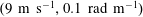 $(9~\text{m}~\text{s}^{-1},0.1~\text{rad}~\text{m}^{-1})$
and
$(9~\text{m}~\text{s}^{-1},0.1~\text{rad}~\text{m}^{-1})$
and
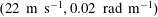 $(22~\text{m}~\text{s}^{-1},0.02~\text{rad}~\text{m}^{-1})$
for a wave whose wavelength is 5 m, 50 m and 300 m, respectively. For any variable
$(22~\text{m}~\text{s}^{-1},0.02~\text{rad}~\text{m}^{-1})$
for a wave whose wavelength is 5 m, 50 m and 300 m, respectively. For any variable
 $\unicode[STIX]{x1D711}$
, its perturbation series is denoted as
$\unicode[STIX]{x1D711}$
, its perturbation series is denoted as
 $$\begin{eqnarray}\unicode[STIX]{x1D711}=\mathop{\sum }_{n}\unicode[STIX]{x1D711}^{[n]},\end{eqnarray}$$
where
 $n$
is an integer index and the superscript
$n$
is an integer index and the superscript
 $[n]$
denotes the
$[n]$
denotes the
 $n$
th term of the series. When the
$n$
th term of the series. When the
 $n$
th term is non-dimensionalised with
$n$
th term is non-dimensionalised with
 $k$
and
$k$
and
 $c^{[0]}$
, it is at most of
$c^{[0]}$
, it is at most of
 $O(\unicode[STIX]{x1D716}^{n})$
, where
$O(\unicode[STIX]{x1D716}^{n})$
, where
 $\unicode[STIX]{x1D716}\equiv 0.1$
in S19. Note that
$\unicode[STIX]{x1D716}\equiv 0.1$
in S19. Note that
 $\unicode[STIX]{x1D716}$
is defined as 0.1 for two reasons. Firstly, specifying a value of
$\unicode[STIX]{x1D716}$
is defined as 0.1 for two reasons. Firstly, specifying a value of
 $\unicode[STIX]{x1D716}$
is necessary to evaluate the orders of the coefficients contained in some terms of the governing equations. Secondly, this definition keeps the notation simple because it then allows the order of any quantity appearing in S19 to be expressed in terms of
$\unicode[STIX]{x1D716}$
is necessary to evaluate the orders of the coefficients contained in some terms of the governing equations. Secondly, this definition keeps the notation simple because it then allows the order of any quantity appearing in S19 to be expressed in terms of
 $\unicode[STIX]{x1D716}$
. In general, one may wish to introduce multiple scaling symbols: e.g. one for the wave amplitude and another for the current speeds. However, this is unnecessary here because S19 considers only a (typical oceanic) condition where the wave amplitude is of
$\unicode[STIX]{x1D716}$
. In general, one may wish to introduce multiple scaling symbols: e.g. one for the wave amplitude and another for the current speeds. However, this is unnecessary here because S19 considers only a (typical oceanic) condition where the wave amplitude is of
 $O(0.1k^{-1})$
and the current speeds are, at most, of
$O(0.1k^{-1})$
and the current speeds are, at most, of
 $O(0.1^{2}c^{[0]})$
. (Note that common current speeds relevant to oceanic submesoscale and Langmuir circulations are of order of
$O(0.1^{2}c^{[0]})$
. (Note that common current speeds relevant to oceanic submesoscale and Langmuir circulations are of order of
 $1{-}10~\text{cm}~\text{s}^{-1}$
(e.g. Suzuki et al.
Reference Suzuki, Fox-Kemper, Hamlington and Van Roekel2016), neglecting the intermittent currents that may be produced by wave breaking.) More details are given in § 3.1.
$1{-}10~\text{cm}~\text{s}^{-1}$
(e.g. Suzuki et al.
Reference Suzuki, Fox-Kemper, Hamlington and Van Roekel2016), neglecting the intermittent currents that may be produced by wave breaking.) More details are given in § 3.1.
2.2 Flow components
Throughout this paper, the following subscript indices are used for the tensor indices:
 $H=1,2$
;
$H=1,2$
;
 $h=1,2$
;
$h=1,2$
;
 $i=1,2,3$
; and
$i=1,2,3$
; and
 $\ell =1,2,3,t$
. Here, 1 and 2 are for the horizontal dimensions, 3 is for the vertical dimension, and
$\ell =1,2,3,t$
. Here, 1 and 2 are for the horizontal dimensions, 3 is for the vertical dimension, and
 $t$
is for the time dimension. The Einstein summation convention is used throughout. At any position in the water, the fluid velocity
$t$
is for the time dimension. The Einstein summation convention is used throughout. At any position in the water, the fluid velocity
 $(u_{1},u_{2},u_{3})\equiv (u,v,w)$
consists solely of the current velocity
$(u_{1},u_{2},u_{3})\equiv (u,v,w)$
consists solely of the current velocity
 $(u_{1}^{c},u_{2}^{c},u_{3}^{c})\equiv (u^{c},v^{c},w^{c})$
and the wave velocity
$(u_{1}^{c},u_{2}^{c},u_{3}^{c})\equiv (u^{c},v^{c},w^{c})$
and the wave velocity
 $(u_{1}^{w},u_{2}^{w},u_{3}^{w})\equiv (u^{w},v^{w},w^{w})$
: that is,
$(u_{1}^{w},u_{2}^{w},u_{3}^{w})\equiv (u^{w},v^{w},w^{w})$
: that is,
 $u_{i}=u_{i}^{c}+u_{i}^{w}$
. Every point of the physical Euclidean space is given both a Cartesian coordinate
$u_{i}=u_{i}^{c}+u_{i}^{w}$
. Every point of the physical Euclidean space is given both a Cartesian coordinate
 $(x,y,z)$
and a surface-following coordinate
$(x,y,z)$
and a surface-following coordinate
 $(x,y,\unicode[STIX]{x1D701})$
, as illustrated in figure 1. The horizontal coordinate system of the surface-following coordinate system is identical to the Cartesian one. The surface labelled with a constant value of
$(x,y,\unicode[STIX]{x1D701})$
, as illustrated in figure 1. The horizontal coordinate system of the surface-following coordinate system is identical to the Cartesian one. The surface labelled with a constant value of
 $\unicode[STIX]{x1D701}$
follows the vertical displacement due to the wave motion, as detailed in § 2.3.
$\unicode[STIX]{x1D701}$
follows the vertical displacement due to the wave motion, as detailed in § 2.3.
All velocities are measured with respect to the Cartesian coordinate system, and the directions of
 $u$
,
$u$
,
 $v$
and
$v$
and
 $w$
are the same as the directions of
$w$
are the same as the directions of
 $x$
,
$x$
,
 $y$
and
$y$
and
 $z$
, respectively, even when the position of a velocity is indicated with
$z$
, respectively, even when the position of a velocity is indicated with
 $(x,y,\unicode[STIX]{x1D701})$
. That is,
$(x,y,\unicode[STIX]{x1D701})$
. That is,
 $u_{i}(x,y,\unicode[STIX]{x1D701},t)=u_{i}(x,y,z(x,y,\unicode[STIX]{x1D701},t),t)$
, where
$u_{i}(x,y,\unicode[STIX]{x1D701},t)=u_{i}(x,y,z(x,y,\unicode[STIX]{x1D701},t),t)$
, where
 $z(x,y,\unicode[STIX]{x1D701},t)$
is the Cartesian vertical coordinate of the position indicated by
$z(x,y,\unicode[STIX]{x1D701},t)$
is the Cartesian vertical coordinate of the position indicated by
 $(x,y,\unicode[STIX]{x1D701},t)$
. In other words, the velocity of a fluid parcel is described using the Cartesian velocity components, and its position is indicated using a surface-following curvilinear coordinate system. This approach is commonly used in interfacial or boundary-layer problems (e.g. Hsu et al.
Reference Hsu, Hsu and Street1981; Hunt, Leibovich & Richards Reference Hunt, Leibovich and Richards1988; Belcher & Hunt Reference Belcher and Hunt1993) involving a surface undulation, when it is desirable to distinguish the momentum (e.g. current) extrinsic to the surface undulation from that (e.g. wave) intrinsic to the surface undulation. This distinction can be often most meaningfully made with respect to a Cartesian basis while taking into account the material-surface displacement induced by the flow intrinsic to the surface undulation. Moreover, this description facilitates interpretation of observational data (Hsu et al.
Reference Hsu, Hsu and Street1981). A detailed discussion on the advantages of this approach over other coordinate systems or other velocity descriptions is given in Hsu et al. (Reference Hsu, Hsu and Street1981).
$(x,y,\unicode[STIX]{x1D701},t)$
. In other words, the velocity of a fluid parcel is described using the Cartesian velocity components, and its position is indicated using a surface-following curvilinear coordinate system. This approach is commonly used in interfacial or boundary-layer problems (e.g. Hsu et al.
Reference Hsu, Hsu and Street1981; Hunt, Leibovich & Richards Reference Hunt, Leibovich and Richards1988; Belcher & Hunt Reference Belcher and Hunt1993) involving a surface undulation, when it is desirable to distinguish the momentum (e.g. current) extrinsic to the surface undulation from that (e.g. wave) intrinsic to the surface undulation. This distinction can be often most meaningfully made with respect to a Cartesian basis while taking into account the material-surface displacement induced by the flow intrinsic to the surface undulation. Moreover, this description facilitates interpretation of observational data (Hsu et al.
Reference Hsu, Hsu and Street1981). A detailed discussion on the advantages of this approach over other coordinate systems or other velocity descriptions is given in Hsu et al. (Reference Hsu, Hsu and Street1981).
Consider a deep-water surface gravity wave field whose leading-order displacement of the water surface is given by
 $a(x,y,t)\cos \unicode[STIX]{x1D712}$
. Here,
$a(x,y,t)\cos \unicode[STIX]{x1D712}$
. Here,
 $a$
is the amplitude and
$a$
is the amplitude and
 $\unicode[STIX]{x1D712}$
is defined as
$\unicode[STIX]{x1D712}$
is defined as
 $$\begin{eqnarray}\unicode[STIX]{x1D712}\equiv s(x,y,t)-\unicode[STIX]{x1D6E9},\end{eqnarray}$$
where
 $s(x,y,t)$
is the phase function and
$s(x,y,t)$
is the phase function and
 $\unicode[STIX]{x1D6E9}$
is the phase shift parameter. The phase shift parameter is a real variable and is independent of the coordinate variables. The wavenumber
$\unicode[STIX]{x1D6E9}$
is the phase shift parameter. The phase shift parameter is a real variable and is independent of the coordinate variables. The wavenumber
 $k\hat{k}_{h}$
and the apparent frequency
$k\hat{k}_{h}$
and the apparent frequency
 $k(c+\hat{k}_{h}u_{h}^{D})$
are defined as
$k(c+\hat{k}_{h}u_{h}^{D})$
are defined as
 $$\begin{eqnarray}k\hat{k}_{h}\equiv \unicode[STIX]{x2202}_{h}s=\unicode[STIX]{x2202}_{h}\unicode[STIX]{x1D712},\quad k(c+\hat{k}_{h}u_{h}^{D})\equiv -\unicode[STIX]{x2202}_{t}s=-\unicode[STIX]{x2202}_{t}\unicode[STIX]{x1D712},\end{eqnarray}$$
where
 $(\hat{k}_{1},\hat{k}_{2})$
is the unit vector of the wavenumber and
$(\hat{k}_{1},\hat{k}_{2})$
is the unit vector of the wavenumber and
 $(u_{1}^{D},u_{2}^{D})$
is the Doppler shift velocity. From these definitions, it is evident that
$(u_{1}^{D},u_{2}^{D})$
is the Doppler shift velocity. From these definitions, it is evident that
 $a$
,
$a$
,
 $k$
,
$k$
,
 $\hat{k}_{h}$
,
$\hat{k}_{h}$
,
 $c$
and
$c$
and
 $u_{h}^{D}$
are independent of
$u_{h}^{D}$
are independent of
 $\unicode[STIX]{x1D6E9}$
,
$\unicode[STIX]{x1D6E9}$
,
 $z$
and
$z$
and
 $\unicode[STIX]{x1D701}$
. The apparent frequency or equivalently
$\unicode[STIX]{x1D701}$
. The apparent frequency or equivalently
 $c$
and
$c$
and
 $u_{h}^{D}$
are unknown variables to be determined as part of the wave solutions.
$u_{h}^{D}$
are unknown variables to be determined as part of the wave solutions.
The wave solutions sought correct to
 $O(\unicode[STIX]{x1D716}^{3})$
in § 5 are functions of
$O(\unicode[STIX]{x1D716}^{3})$
in § 5 are functions of
 $(x,y,\unicode[STIX]{x1D701},t,\unicode[STIX]{x1D6E9})$
and periodic in
$(x,y,\unicode[STIX]{x1D701},t,\unicode[STIX]{x1D6E9})$
and periodic in
 $\unicode[STIX]{x1D6E9}$
, that is,
$\unicode[STIX]{x1D6E9}$
, that is,
 $$\begin{eqnarray}u_{i}^{w}(x,y,\unicode[STIX]{x1D701},t,\unicode[STIX]{x1D6E9})=u_{i}^{w}(x,y,\unicode[STIX]{x1D701},t,\unicode[STIX]{x1D6E9}+2\unicode[STIX]{x03C0}).\end{eqnarray}$$
Importantly, a periodicity in time or space is not required. Hence, the amplitude or wavenumber can change in time and space. Because the wave solutions at any value of
 $\unicode[STIX]{x1D6E9}$
satisfy the governing equations,
$\unicode[STIX]{x1D6E9}$
satisfy the governing equations,
 $u_{i}^{w}(x,y,\unicode[STIX]{x1D701},t,\unicode[STIX]{x1D6E9})$
represents a one-parameter family of solutions which are all valid at
$u_{i}^{w}(x,y,\unicode[STIX]{x1D701},t,\unicode[STIX]{x1D6E9})$
represents a one-parameter family of solutions which are all valid at
 $(x,y,\unicode[STIX]{x1D701},t)$
. Denote the averaging over this solution family at a coordinate
$(x,y,\unicode[STIX]{x1D701},t)$
. Denote the averaging over this solution family at a coordinate
 $(x,y,\unicode[STIX]{x1D701},t)$
by
$(x,y,\unicode[STIX]{x1D701},t)$
by
 $$\begin{eqnarray}\langle \unicode[STIX]{x1D711}\rangle (x,y,\unicode[STIX]{x1D701},t)\equiv \frac{1}{2\unicode[STIX]{x03C0}}\int _{0}^{2\unicode[STIX]{x03C0}}\unicode[STIX]{x1D711}(x,y,\unicode[STIX]{x1D701},t,\unicode[STIX]{x1D6E9})\,\text{d}\unicode[STIX]{x1D6E9}\end{eqnarray}$$
for any function
 $\unicode[STIX]{x1D711}$
. Crucially,
$\unicode[STIX]{x1D711}$
. Crucially,
 $\langle ~\rangle$
exactly commutes with the spatial and temporal partial differentiation operators with respect to
$\langle ~\rangle$
exactly commutes with the spatial and temporal partial differentiation operators with respect to
 $(x,y,\unicode[STIX]{x1D701},t)$
. (In contrast,
$(x,y,\unicode[STIX]{x1D701},t)$
. (In contrast,
 $\langle ~\rangle$
may not commute with the partial differentiation operators with respect to
$\langle ~\rangle$
may not commute with the partial differentiation operators with respect to
 $(x,y,z,t)$
because the averaging
$(x,y,z,t)$
because the averaging
 $\langle ~\rangle$
is not done at a fixed
$\langle ~\rangle$
is not done at a fixed
 $(x,y,z,t)$
.) Moreover,
$(x,y,z,t)$
.) Moreover,
 $\langle ~\rangle$
is idempotent:
$\langle ~\rangle$
is idempotent:
 $\langle \langle \unicode[STIX]{x1D711}\rangle \rangle =\langle \unicode[STIX]{x1D711}\rangle$
. If
$\langle \langle \unicode[STIX]{x1D711}\rangle \rangle =\langle \unicode[STIX]{x1D711}\rangle$
. If
 $\unicode[STIX]{x1D711}$
is independent of
$\unicode[STIX]{x1D711}$
is independent of
 $\unicode[STIX]{x1D6E9}$
, then
$\unicode[STIX]{x1D6E9}$
, then
 $\langle \unicode[STIX]{x1D711}\rangle =\unicode[STIX]{x1D711}$
. These properties are essential for mathematical rigour. Physically,
$\langle \unicode[STIX]{x1D711}\rangle =\unicode[STIX]{x1D711}$
. These properties are essential for mathematical rigour. Physically,
 $\langle ~\rangle$
represents the ensemble averaging at a given
$\langle ~\rangle$
represents the ensemble averaging at a given
 $(x,y,\unicode[STIX]{x1D701},t)$
over the ensemble of states having the same current and wave properties (i.e.
$(x,y,\unicode[STIX]{x1D701},t)$
over the ensemble of states having the same current and wave properties (i.e.
 $a$
and
$a$
and
 $s$
) but different values of the phase shift parameter
$s$
) but different values of the phase shift parameter
 $\unicode[STIX]{x1D6E9}$
. This use of
$\unicode[STIX]{x1D6E9}$
. This use of
 $\unicode[STIX]{x1D6E9}$
follows that of Hayes (Reference Hayes1970) and Grimshaw (Reference Grimshaw1984). The wave motion consists of the ensemble average
$\unicode[STIX]{x1D6E9}$
follows that of Hayes (Reference Hayes1970) and Grimshaw (Reference Grimshaw1984). The wave motion consists of the ensemble average
 $\mathfrak{U}_{i}\equiv \langle u_{i}^{w}\rangle$
and the oscillatory deviations from it, that is,
$\mathfrak{U}_{i}\equiv \langle u_{i}^{w}\rangle$
and the oscillatory deviations from it, that is,
 $$\begin{eqnarray}u_{i}^{w}(x,y,\unicode[STIX]{x1D701},t,\unicode[STIX]{x1D6E9})=\mathfrak{U}_{i}(x,y,\unicode[STIX]{x1D701},t)+[u_{i}^{w}(x,y,\unicode[STIX]{x1D701},t,\unicode[STIX]{x1D6E9})-\mathfrak{U}_{i}(x,y,\unicode[STIX]{x1D701},t)].\end{eqnarray}$$
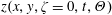
2.3 Coordinate systems
Let us call the surface-following coordinate system the
 $\unicode[STIX]{x1D701}$
-coordinate system. Recall that
$\unicode[STIX]{x1D701}$
-coordinate system. Recall that
 $(x,y,t,\unicode[STIX]{x1D6E9})$
are identical between the Cartesian and
$(x,y,t,\unicode[STIX]{x1D6E9})$
are identical between the Cartesian and
 $\unicode[STIX]{x1D701}$
-coordinate systems. Also recall that the
$\unicode[STIX]{x1D701}$
-coordinate systems. Also recall that the
 $z$
-coordinate – i.e. the height – of a point
$z$
-coordinate – i.e. the height – of a point
 $(x,y,\unicode[STIX]{x1D701},t,\unicode[STIX]{x1D6E9})$
is
$(x,y,\unicode[STIX]{x1D701},t,\unicode[STIX]{x1D6E9})$
is
 $z(x,y,\unicode[STIX]{x1D701},t,\unicode[STIX]{x1D6E9})$
. Hereafter, let us use the following notation: for any variable
$z(x,y,\unicode[STIX]{x1D701},t,\unicode[STIX]{x1D6E9})$
. Hereafter, let us use the following notation: for any variable
 $\unicode[STIX]{x1D711}$
,
$\unicode[STIX]{x1D711}$
,
 $$\begin{eqnarray}\displaystyle & \displaystyle \unicode[STIX]{x2202}_{\ell }^{z}\unicode[STIX]{x1D711}\equiv \frac{\unicode[STIX]{x2202}\unicode[STIX]{x1D711}(x,y,z,t,\unicode[STIX]{x1D6E9})}{\unicode[STIX]{x2202}x_{\ell }}\quad \text{where }(x_{1},x_{2},x_{3},x_{t})\equiv (x,y,z,t), & \displaystyle\end{eqnarray}$$
 $$\begin{eqnarray}\displaystyle & \displaystyle \unicode[STIX]{x2202}_{\ell }^{\unicode[STIX]{x1D701}}\unicode[STIX]{x1D711}\equiv \frac{\unicode[STIX]{x2202}\unicode[STIX]{x1D711}(x,y,\unicode[STIX]{x1D701},t,\unicode[STIX]{x1D6E9})}{\unicode[STIX]{x2202}x_{\ell }}\quad \text{where }(x_{1},x_{2},x_{3},x_{t})\equiv (x,y,\unicode[STIX]{x1D701},t). & \displaystyle\end{eqnarray}$$
Multiple operations are denoted by
 $(\unicode[STIX]{x2202}_{\ell }^{\unicode[STIX]{x1D701}})^{n}$
, e.g.
$(\unicode[STIX]{x2202}_{\ell }^{\unicode[STIX]{x1D701}})^{n}$
, e.g.
 $(\unicode[STIX]{x2202}_{2}^{\unicode[STIX]{x1D701}})^{2}\equiv \unicode[STIX]{x2202}_{2}^{\unicode[STIX]{x1D701}}\unicode[STIX]{x2202}_{2}^{\unicode[STIX]{x1D701}}$
. Because
$(\unicode[STIX]{x2202}_{2}^{\unicode[STIX]{x1D701}})^{2}\equiv \unicode[STIX]{x2202}_{2}^{\unicode[STIX]{x1D701}}\unicode[STIX]{x2202}_{2}^{\unicode[STIX]{x1D701}}$
. Because
 $a$
,
$a$
,
 $k$
,
$k$
,
 $\hat{k}_{h}$
,
$\hat{k}_{h}$
,
 $c$
and
$c$
and
 $u_{h}^{D}$
are functions only of
$u_{h}^{D}$
are functions only of
 $(x,y,t)$
, their derivatives do not have the superscript
$(x,y,t)$
, their derivatives do not have the superscript
 $z$
or
$z$
or
 $\unicode[STIX]{x1D701}$
on
$\unicode[STIX]{x1D701}$
on
 $\unicode[STIX]{x2202}_{\ell }$
.
$\unicode[STIX]{x2202}_{\ell }$
.
Now, let us more precisely define the constant-
 $\unicode[STIX]{x1D701}$
surfaces to be used as the
$\unicode[STIX]{x1D701}$
surfaces to be used as the
 $\unicode[STIX]{x1D701}$
-coordinates. First, let the water surface be the constant-
$\unicode[STIX]{x1D701}$
-coordinates. First, let the water surface be the constant-
 $\unicode[STIX]{x1D701}$
surface labelled with
$\unicode[STIX]{x1D701}$
surface labelled with
 $\unicode[STIX]{x1D701}=0$
. Then, the height of the water surface – namely,
$\unicode[STIX]{x1D701}=0$
. Then, the height of the water surface – namely,
 $z(x,y,\unicode[STIX]{x1D701}=0,t,\unicode[STIX]{x1D6E9})$
– satisfies
$z(x,y,\unicode[STIX]{x1D701}=0,t,\unicode[STIX]{x1D6E9})$
– satisfies
 $\unicode[STIX]{x2202}_{t}^{\unicode[STIX]{x1D701}}z=w-u_{h}\unicode[STIX]{x2202}_{h}^{\unicode[STIX]{x1D701}}z$
. This is the standard kinematic boundary condition for the free surface. In S19, let us limit our consideration to only those currents whose vertical velocities
$\unicode[STIX]{x2202}_{t}^{\unicode[STIX]{x1D701}}z=w-u_{h}\unicode[STIX]{x2202}_{h}^{\unicode[STIX]{x1D701}}z$
. This is the standard kinematic boundary condition for the free surface. In S19, let us limit our consideration to only those currents whose vertical velocities
 $w^{c}$
are zero at the water surface. That is,
$w^{c}$
are zero at the water surface. That is,
 $w=w^{w}$
at the water surface. Therefore, the water surface satisfies
$w=w^{w}$
at the water surface. Therefore, the water surface satisfies
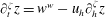 $\unicode[STIX]{x2202}_{t}^{\unicode[STIX]{x1D701}}z=w^{w}-u_{h}\unicode[STIX]{x2202}_{h}^{\unicode[STIX]{x1D701}}z$
. Now, let us define every constant-
$\unicode[STIX]{x2202}_{t}^{\unicode[STIX]{x1D701}}z=w^{w}-u_{h}\unicode[STIX]{x2202}_{h}^{\unicode[STIX]{x1D701}}z$
. Now, let us define every constant-
 $\unicode[STIX]{x1D701}$
surface in the interior by the following equation for its
$\unicode[STIX]{x1D701}$
surface in the interior by the following equation for its
 $z$
-coordinate
$z$
-coordinate
 $z(x,y,\unicode[STIX]{x1D701},t,\unicode[STIX]{x1D6E9})$
:
$z(x,y,\unicode[STIX]{x1D701},t,\unicode[STIX]{x1D6E9})$
:
 $$\begin{eqnarray}\unicode[STIX]{x2202}_{t}^{\unicode[STIX]{x1D701}}z=w^{w}-u_{h}\unicode[STIX]{x2202}_{h}^{\unicode[STIX]{x1D701}}z.\end{eqnarray}$$
Here any initial condition or constant of integration should be chosen so that the constant-
 $\unicode[STIX]{x1D701}$
surfaces become identical to the constant-
$\unicode[STIX]{x1D701}$
surfaces become identical to the constant-
 $z$
surfaces in the absence of waves (or any other disturbances such as geostrophically balanced surface tilts, which are negligible at the orders concerned in S19). If
$z$
surfaces in the absence of waves (or any other disturbances such as geostrophically balanced surface tilts, which are negligible at the orders concerned in S19). If
 $w^{w}$
in (2.9) is replaced with
$w^{w}$
in (2.9) is replaced with
 $w$
, then the constant-
$w$
, then the constant-
 $\unicode[STIX]{x1D701}$
surfaces defined in this way are the interior material surfaces. However, (2.9) uses
$\unicode[STIX]{x1D701}$
surfaces defined in this way are the interior material surfaces. However, (2.9) uses
 $w^{w}$
so that the constant-
$w^{w}$
so that the constant-
 $\unicode[STIX]{x1D701}$
surfaces follow the displacement due to the wave vertical velocities, rather than the fluid vertical velocities. Thus, current vertical velocity
$\unicode[STIX]{x1D701}$
surfaces follow the displacement due to the wave vertical velocities, rather than the fluid vertical velocities. Thus, current vertical velocity
 $w^{c}$
, which may be of
$w^{c}$
, which may be of
 $O(\unicode[STIX]{x1D716}^{2}c^{[0]})$
in the interior, goes through (i.e. does not move) the constant-
$O(\unicode[STIX]{x1D716}^{2}c^{[0]})$
in the interior, goes through (i.e. does not move) the constant-
 $\unicode[STIX]{x1D701}$
surfaces. Note that the kinematic boundary condition for the water surface is the same as (2.9) at
$\unicode[STIX]{x1D701}$
surfaces. Note that the kinematic boundary condition for the water surface is the same as (2.9) at
 $\unicode[STIX]{x1D701}=0$
.
$\unicode[STIX]{x1D701}=0$
.
In S19, the amplitude is of first order, i.e.
 $a=O(\unicode[STIX]{x1D716}k^{-1})$
. Therefore, the perturbation series of
$a=O(\unicode[STIX]{x1D716}k^{-1})$
. Therefore, the perturbation series of
 $z(x,y,\unicode[STIX]{x1D701},t,\unicode[STIX]{x1D6E9})$
is
$z(x,y,\unicode[STIX]{x1D701},t,\unicode[STIX]{x1D6E9})$
is
 $$\begin{eqnarray}z(x,y,\unicode[STIX]{x1D701},t,\unicode[STIX]{x1D6E9})=\unicode[STIX]{x1D701}+\mathop{\sum }_{n\geqslant 1}z^{[n]}(x,y,\unicode[STIX]{x1D701},t,\unicode[STIX]{x1D6E9}),\end{eqnarray}$$
where
 $z^{[n]}\leqslant O(\unicode[STIX]{x1D716}^{n}k^{-1})$
. The value of
$z^{[n]}\leqslant O(\unicode[STIX]{x1D716}^{n}k^{-1})$
. The value of
 $\unicode[STIX]{x1D701}$
is equal to the unperturbed height and
$\unicode[STIX]{x1D701}$
is equal to the unperturbed height and
 $\sum z^{[n]}$
is the perturbation.
$\sum z^{[n]}$
is the perturbation.
Let us define the constant-
 $\unicode[STIX]{x1D701}$
layer containing a point
$\unicode[STIX]{x1D701}$
layer containing a point
 $(x,y,\unicode[STIX]{x1D701},t,\unicode[STIX]{x1D6E9})$
as the layer containing the point and bounded by two infinitesimally close constant-
$(x,y,\unicode[STIX]{x1D701},t,\unicode[STIX]{x1D6E9})$
as the layer containing the point and bounded by two infinitesimally close constant-
 $\unicode[STIX]{x1D701}$
surfaces. The concept of a layer is useful because the wave motion undulates both the slope and thickness of a material layer. The constant-
$\unicode[STIX]{x1D701}$
surfaces. The concept of a layer is useful because the wave motion undulates both the slope and thickness of a material layer. The constant-
 $\unicode[STIX]{x1D701}$
surface and layer at
$\unicode[STIX]{x1D701}$
surface and layer at
 $(x,y,\unicode[STIX]{x1D701},t,\unicode[STIX]{x1D6E9})$
have the following properties:
$(x,y,\unicode[STIX]{x1D701},t,\unicode[STIX]{x1D6E9})$
have the following properties:
 $$\begin{eqnarray}\displaystyle & \displaystyle \text{vertical motion of the surface,}\quad S_{t}\equiv \unicode[STIX]{x2202}_{t}^{\unicode[STIX]{x1D701}}z=\unicode[STIX]{x2202}_{t}^{\unicode[STIX]{x1D701}}\mathop{\sum }_{n\geqslant 1}z^{[n]}, & \displaystyle\end{eqnarray}$$
 $$\begin{eqnarray}\displaystyle & \displaystyle \text{slope of the surface,}\quad S_{h}\equiv \unicode[STIX]{x2202}_{h}^{\unicode[STIX]{x1D701}}z=\unicode[STIX]{x2202}_{h}^{\unicode[STIX]{x1D701}}\mathop{\sum }_{n\geqslant 1}z^{[n]}, & \displaystyle\end{eqnarray}$$
 $$\begin{eqnarray}\displaystyle & \displaystyle \text{layer-thickness perturbation,}\quad S_{3}\equiv \unicode[STIX]{x2202}_{3}^{\unicode[STIX]{x1D701}}\mathop{\sum }_{n\geqslant 1}z^{[n]}, & \displaystyle\end{eqnarray}$$
 $$\begin{eqnarray}\displaystyle & \displaystyle \text{normalised layer thickness,}\quad J\equiv \unicode[STIX]{x2202}_{3}^{\unicode[STIX]{x1D701}}z=1+S_{3}. & \displaystyle\end{eqnarray}$$
Here
 $J$
is the layer thickness normalised with the undeformed thickness and is also the Jacobian determinant (i.e.
$J$
is the layer thickness normalised with the undeformed thickness and is also the Jacobian determinant (i.e.
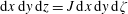 $\text{d}x\,\text{d}y\,\text{d}z=J\,\text{d}x\,\text{d}y\,\text{d}\unicode[STIX]{x1D701}$
). The commutation of the differential operators yields the following identities:
$\text{d}x\,\text{d}y\,\text{d}z=J\,\text{d}x\,\text{d}y\,\text{d}\unicode[STIX]{x1D701}$
). The commutation of the differential operators yields the following identities:
 $\unicode[STIX]{x2202}_{\ell }^{\unicode[STIX]{x1D701}}J=\unicode[STIX]{x2202}_{\ell }^{\unicode[STIX]{x1D701}}S_{3}$
and
$\unicode[STIX]{x2202}_{\ell }^{\unicode[STIX]{x1D701}}J=\unicode[STIX]{x2202}_{\ell }^{\unicode[STIX]{x1D701}}S_{3}$
and
 $\unicode[STIX]{x2202}_{\ell }^{\unicode[STIX]{x1D701}}S_{m}=\unicode[STIX]{x2202}_{m}^{\unicode[STIX]{x1D701}}S_{\ell }$
for
$\unicode[STIX]{x2202}_{\ell }^{\unicode[STIX]{x1D701}}S_{m}=\unicode[STIX]{x2202}_{m}^{\unicode[STIX]{x1D701}}S_{\ell }$
for
 $m=1,2,3,t$
.
$m=1,2,3,t$
.
Since
 $\unicode[STIX]{x2202}_{3}^{z}x$
,
$\unicode[STIX]{x2202}_{3}^{z}x$
,
 $\unicode[STIX]{x2202}_{3}^{z}y$
and
$\unicode[STIX]{x2202}_{3}^{z}y$
and
 $\unicode[STIX]{x2202}_{3}^{z}t$
are all zero, the standard chain rule for
$\unicode[STIX]{x2202}_{3}^{z}t$
are all zero, the standard chain rule for
 $\unicode[STIX]{x2202}_{3}^{z}$
yields
$\unicode[STIX]{x2202}_{3}^{z}$
yields
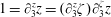 $1=\unicode[STIX]{x2202}_{3}^{z}z=(\unicode[STIX]{x2202}_{3}^{z}\unicode[STIX]{x1D701})\unicode[STIX]{x2202}_{3}^{\unicode[STIX]{x1D701}}z$
. Therefore,
$1=\unicode[STIX]{x2202}_{3}^{z}z=(\unicode[STIX]{x2202}_{3}^{z}\unicode[STIX]{x1D701})\unicode[STIX]{x2202}_{3}^{\unicode[STIX]{x1D701}}z$
. Therefore,
 $J^{-1}=\unicode[STIX]{x2202}_{3}^{z}\unicode[STIX]{x1D701}$
. Then, the chain rules for
$J^{-1}=\unicode[STIX]{x2202}_{3}^{z}\unicode[STIX]{x1D701}$
. Then, the chain rules for
 $\unicode[STIX]{x2202}_{3}^{z}$
and
$\unicode[STIX]{x2202}_{3}^{z}$
and
 $\unicode[STIX]{x2202}_{\ell }^{\unicode[STIX]{x1D701}}$
yield
$\unicode[STIX]{x2202}_{\ell }^{\unicode[STIX]{x1D701}}$
yield
 $$\begin{eqnarray}\unicode[STIX]{x2202}_{3}^{z}\unicode[STIX]{x1D711}=(\unicode[STIX]{x2202}_{3}^{z}\unicode[STIX]{x1D701})\unicode[STIX]{x2202}_{3}^{\unicode[STIX]{x1D701}}\unicode[STIX]{x1D711}=J^{-1}\unicode[STIX]{x2202}_{3}^{\unicode[STIX]{x1D701}}\unicode[STIX]{x1D711}\quad \text{and}\quad \unicode[STIX]{x2202}_{\ell }^{z}=\unicode[STIX]{x2202}_{\ell }^{\unicode[STIX]{x1D701}}-S_{\ell }J^{-1}\unicode[STIX]{x2202}_{3}^{\unicode[STIX]{x1D701}}.\end{eqnarray}$$
2.4 Equations of motion
Hereafter, consider an inviscid and incompressible fluid having a uniform density
 $\unicode[STIX]{x1D70C}_{0}$
. Thus, the equations of motion with respect to the Cartesian coordinate system are
$\unicode[STIX]{x1D70C}_{0}$
. Thus, the equations of motion with respect to the Cartesian coordinate system are
 $$\begin{eqnarray}\displaystyle & \displaystyle \unicode[STIX]{x2202}_{t}^{z}u_{i}+u_{h}\unicode[STIX]{x2202}_{h}^{z}u_{i}+w\unicode[STIX]{x2202}_{3}^{z}u_{i}=-\unicode[STIX]{x2202}_{i}^{z}P, & \displaystyle\end{eqnarray}$$
 $$\begin{eqnarray}\displaystyle & \displaystyle \unicode[STIX]{x2202}_{i}^{z}u_{i}=0, & \displaystyle\end{eqnarray}$$
where
 $P\equiv p/\unicode[STIX]{x1D70C}_{0}+gz$
, with
$P\equiv p/\unicode[STIX]{x1D70C}_{0}+gz$
, with
 $p$
the pressure and
$p$
the pressure and
 $g$
the gravitational acceleration. According to (2.15) and
$g$
the gravitational acceleration. According to (2.15) and
 $w=w^{c}+w^{w}$
, (2.16) and (2.17) are equivalent to
$w=w^{c}+w^{w}$
, (2.16) and (2.17) are equivalent to
 $$\begin{eqnarray}\displaystyle & \displaystyle \text{momentum equations,}\quad \unicode[STIX]{x2202}_{t}^{\unicode[STIX]{x1D701}}u_{i}+u_{h}\unicode[STIX]{x2202}_{h}^{\unicode[STIX]{x1D701}}u_{i}+w^{c}J^{-1}\unicode[STIX]{x2202}_{3}^{\unicode[STIX]{x1D701}}u_{i}=-\unicode[STIX]{x2202}_{i}^{\unicode[STIX]{x1D701}}P+S_{i}J^{-1}\unicode[STIX]{x2202}_{3}^{\unicode[STIX]{x1D701}}P, & \displaystyle\end{eqnarray}$$
 $$\begin{eqnarray}\displaystyle & \displaystyle \text{incompressibility,}\quad \unicode[STIX]{x2202}_{i}^{\unicode[STIX]{x1D701}}u_{i}-S_{i}J^{-1}\unicode[STIX]{x2202}_{3}^{\unicode[STIX]{x1D701}}u_{i}=0. & \displaystyle\end{eqnarray}$$
The lower and upper boundary conditions for deep-water waves without wind forcing are
 $$\begin{eqnarray}\displaystyle & \displaystyle u_{i}^{w}=0\quad \text{at }\unicode[STIX]{x1D701}=-\infty , & \displaystyle\end{eqnarray}$$
 $$\begin{eqnarray}\displaystyle & \displaystyle \frac{1}{g}\unicode[STIX]{x2202}_{t}^{\unicode[STIX]{x1D701}}P-w^{w}+u_{h}S_{h}=0\quad \text{at }\unicode[STIX]{x1D701}=0, & \displaystyle\end{eqnarray}$$
where
 $w^{c}=0$
at
$w^{c}=0$
at
 $\unicode[STIX]{x1D701}=0$
in S19. Equation (2.21) is the joint condition between the kinematic upper boundary condition (i.e.
$\unicode[STIX]{x1D701}=0$
in S19. Equation (2.21) is the joint condition between the kinematic upper boundary condition (i.e.
 $\unicode[STIX]{x2202}_{t}^{\unicode[STIX]{x1D701}}z=w-u_{h}\unicode[STIX]{x2202}_{h}^{\unicode[STIX]{x1D701}}z$
) and the dynamic upper boundary condition (i.e.
$\unicode[STIX]{x2202}_{t}^{\unicode[STIX]{x1D701}}z=w-u_{h}\unicode[STIX]{x2202}_{h}^{\unicode[STIX]{x1D701}}z$
) and the dynamic upper boundary condition (i.e.
 $p=\text{const.}$
at
$p=\text{const.}$
at
 $\unicode[STIX]{x1D701}=0$
). The definition of
$\unicode[STIX]{x1D701}=0$
). The definition of
 $P$
and the dynamic upper boundary condition give
$P$
and the dynamic upper boundary condition give
 $\unicode[STIX]{x2202}_{t}^{\unicode[STIX]{x1D701}}P=g\unicode[STIX]{x2202}_{t}^{\unicode[STIX]{x1D701}}z$
at
$\unicode[STIX]{x2202}_{t}^{\unicode[STIX]{x1D701}}P=g\unicode[STIX]{x2202}_{t}^{\unicode[STIX]{x1D701}}z$
at
 $\unicode[STIX]{x1D701}=0$
. Combining this and the kinematic upper boundary condition yields (2.21).
$\unicode[STIX]{x1D701}=0$
. Combining this and the kinematic upper boundary condition yields (2.21).
3 Conditions of the wave field and circulation
3.1 Scaling conditions
S19 considers the following conditions:
 $a=O(\unicode[STIX]{x1D716}k^{-1})$
, to consider a typical non-breaking wave field;
$a=O(\unicode[STIX]{x1D716}k^{-1})$
, to consider a typical non-breaking wave field;
 $\hat{k}_{1}=O(1)$
and
$\hat{k}_{1}=O(1)$
and
 $\hat{k}_{2}\leqslant O(\unicode[STIX]{x1D716})$
, because the wave propagation is roughly in the streamwise direction;
$\hat{k}_{2}\leqslant O(\unicode[STIX]{x1D716})$
, because the wave propagation is roughly in the streamwise direction;
 $\mathfrak{U}_{h}\leqslant O(\unicode[STIX]{x1D716}^{2}\hat{k}_{h}c^{[0]})$
and
$\mathfrak{U}_{h}\leqslant O(\unicode[STIX]{x1D716}^{2}\hat{k}_{h}c^{[0]})$
and
 $\mathfrak{U}_{3}\leqslant O(\unicode[STIX]{x1D716}^{4}c^{[0]})$
, being consistent with a largely uniform and first-order-irrotational wave field; and
$\mathfrak{U}_{3}\leqslant O(\unicode[STIX]{x1D716}^{4}c^{[0]})$
, being consistent with a largely uniform and first-order-irrotational wave field; and
 $u_{i}^{c}\leqslant O(\unicode[STIX]{x1D716}^{2}c^{[0]})$
, like the CL theory. (Higher-order irrotationality of the wave motion is not assumed in S19.) However, unlike the CL theory, S19 does not assume that the current velocity field is non-divergent. Therefore, S19 anticipates a condition
$u_{i}^{c}\leqslant O(\unicode[STIX]{x1D716}^{2}c^{[0]})$
, like the CL theory. (Higher-order irrotationality of the wave motion is not assumed in S19.) However, unlike the CL theory, S19 does not assume that the current velocity field is non-divergent. Therefore, S19 anticipates a condition
 $\unicode[STIX]{x2202}_{i}^{\unicode[STIX]{x1D701}}u_{i}^{c}\leqslant O(\unicode[STIX]{x1D716}^{4}c^{[0]}k)$
, being consistent with the order of
$\unicode[STIX]{x2202}_{i}^{\unicode[STIX]{x1D701}}u_{i}^{c}\leqslant O(\unicode[STIX]{x1D716}^{4}c^{[0]}k)$
, being consistent with the order of
 $\unicode[STIX]{x2202}_{i}^{\unicode[STIX]{x1D701}}\mathfrak{U}_{i}$
. The orders of all other quantities are listed in appendix A. Many of these conditions are roughly depicted in figure 1. Importantly, S19 considers only those current structures whose spanwise widths are wider than roughly one wavelength so that the fourth and higher spanwise derivatives of
$\unicode[STIX]{x2202}_{i}^{\unicode[STIX]{x1D701}}\mathfrak{U}_{i}$
. The orders of all other quantities are listed in appendix A. Many of these conditions are roughly depicted in figure 1. Importantly, S19 considers only those current structures whose spanwise widths are wider than roughly one wavelength so that the fourth and higher spanwise derivatives of
 $u^{c}$
and
$u^{c}$
and
 $w^{c}$
are insignificant compared to their lower spanwise derivatives (see table 4). The anticipated gradients of the wave properties due to the wave–current interaction are specified later in table 5. Note that these scaling conditions are validly possible; that is, these scales are self-consistent with the scales implied by the equations of the wave properties and of the wave-averaged circulation derived later in §§ 5 and 6. An example of the self-consistency conditions is
$w^{c}$
are insignificant compared to their lower spanwise derivatives (see table 4). The anticipated gradients of the wave properties due to the wave–current interaction are specified later in table 5. Note that these scaling conditions are validly possible; that is, these scales are self-consistent with the scales implied by the equations of the wave properties and of the wave-averaged circulation derived later in §§ 5 and 6. An example of the self-consistency conditions is
 $O(\unicode[STIX]{x2202}_{\ell }\unicode[STIX]{x1D711})\geqslant O([c^{[0]}k]^{-1}\unicode[STIX]{x2202}_{t}\unicode[STIX]{x2202}_{\ell }\unicode[STIX]{x1D711})$
for any quantity
$O(\unicode[STIX]{x2202}_{\ell }\unicode[STIX]{x1D711})\geqslant O([c^{[0]}k]^{-1}\unicode[STIX]{x2202}_{t}\unicode[STIX]{x2202}_{\ell }\unicode[STIX]{x1D711})$
for any quantity
 $\unicode[STIX]{x1D711}$
. This is a statement that
$\unicode[STIX]{x1D711}$
. This is a statement that
 $\unicode[STIX]{x2202}_{\ell }\unicode[STIX]{x1D711}$
remains negligible at least during one characteristic period
$\unicode[STIX]{x2202}_{\ell }\unicode[STIX]{x1D711}$
remains negligible at least during one characteristic period
 $(c^{[0]}k)^{-1}$
, if it is initially negligible. To achieve self-consistency, the scales specified here and the results in §§ 5 and 6 are iteratively derived. (This, of course, does not eliminate a possibility of having another validly possible set of scaling conditions.)
$(c^{[0]}k)^{-1}$
, if it is initially negligible. To achieve self-consistency, the scales specified here and the results in §§ 5 and 6 are iteratively derived. (This, of course, does not eliminate a possibility of having another validly possible set of scaling conditions.)
The aforementioned scaling conditions imply an important relationship between the current velocity and its ensemble average (see § A.2 for derivation), namely,
 $$\begin{eqnarray}u_{i}^{c}=\langle u_{i}^{c}\rangle +O(\unicode[STIX]{x1D716}^{4}c^{[0]}).\end{eqnarray}$$
3.2 The class of the current structures assumed in § 5
In § 5, the wave solutions are obtained for a particular class of current structures having the form
 $u^{c}=\sum _{n\geqslant 1}u_{(n)}^{c}$
and
$u^{c}=\sum _{n\geqslant 1}u_{(n)}^{c}$
and
 $w^{c}=\sum _{n\geqslant 1}w_{(n)}^{c}$
where
$w^{c}=\sum _{n\geqslant 1}w_{(n)}^{c}$
where
 $$\begin{eqnarray}\left.\begin{array}{@{}c@{}}u_{(1)}^{c}=C_{\mathbb{A}(1)}{\mathcal{U}}_{(1)}(x,\unicode[STIX]{x1D701},t),\\ u_{(n)}^{c}=B_{\mathbb{A}(n)}\cos \left(\sqrt{K_{\mathbb{A}(n)}^{2}-k^{2}}y+C_{\mathbb{A}(n)}\right){\mathcal{U}}_{(n)}(x,\unicode[STIX]{x1D701},t)\quad \text{for }n\geqslant 2,\end{array}\right\}\end{eqnarray}$$
and
 $$\begin{eqnarray}\left.\begin{array}{@{}c@{}}w_{(1)}^{c}=C_{\mathbb{B}(1)}{\mathcal{W}}_{(1)}(x,\unicode[STIX]{x1D701},t),\\ w_{(n)}^{c}=B_{\mathbb{B}(n)}\cos \left(\sqrt{K_{\mathbb{B}(n)}^{2}-k^{2}}y+C_{\mathbb{B}(n)}\right){\mathcal{W}}_{(n)}(x,\unicode[STIX]{x1D701},t)\quad \text{for }n\geqslant 2.\end{array}\right\}\end{eqnarray}$$
The subscript indices are surrounded with parentheses to avoid possible confusion with the tensor indices. In (3.2) and (3.3),
 $B_{\mathbb{A}(n)}$
,
$B_{\mathbb{A}(n)}$
,
 $C_{\mathbb{A}(n)}$
,
$C_{\mathbb{A}(n)}$
,
 $B_{\mathbb{B}(n)}$
and
$B_{\mathbb{B}(n)}$
and
 $C_{\mathbb{B}(n)}$
are real constants;
$C_{\mathbb{B}(n)}$
are real constants;
 $K_{\mathbb{A}(n)}$
and
$K_{\mathbb{A}(n)}$
and
 $K_{\mathbb{B}(n)}$
(for
$K_{\mathbb{B}(n)}$
(for
 $n\geqslant 2$
) are real parameters in the range of
$n\geqslant 2$
) are real parameters in the range of
 $k<K_{\mathbb{A}(n)}\leqslant 1.15k$
and
$k<K_{\mathbb{A}(n)}\leqslant 1.15k$
and
 $k<K_{\mathbb{B}(n)}\leqslant 1.15k$
(see § A.3 for their scaling conditions); and
$k<K_{\mathbb{B}(n)}\leqslant 1.15k$
(see § A.3 for their scaling conditions); and
 ${\mathcal{U}}_{(n)}$
and
${\mathcal{U}}_{(n)}$
and
 ${\mathcal{W}}_{(n)}$
may be any functions of
${\mathcal{W}}_{(n)}$
may be any functions of
 $(x,\unicode[STIX]{x1D701},t)$
as long as they satisfy the scaling conditions. The upper bound (i.e.
$(x,\unicode[STIX]{x1D701},t)$
as long as they satisfy the scaling conditions. The upper bound (i.e.
 $1.15k$
) of
$1.15k$
) of
 $K_{\mathbb{A}(n)}$
and
$K_{\mathbb{A}(n)}$
and
 $K_{\mathbb{B}(n)}$
gives the narrowest (i.e. 88 % of the wavelength
$K_{\mathbb{B}(n)}$
gives the narrowest (i.e. 88 % of the wavelength
 $2\unicode[STIX]{x03C0}k^{-1}$
) current structure considered in S19. For theoretical consistency,
$2\unicode[STIX]{x03C0}k^{-1}$
) current structure considered in S19. For theoretical consistency,
 $u_{(n)}^{c}$
and
$u_{(n)}^{c}$
and
 $w_{(n)}^{c}$
should individually satisfy the scaling conditions. Figure 2 shows an example.
$w_{(n)}^{c}$
should individually satisfy the scaling conditions. Figure 2 shows an example.

Figure 2. An example of the current structures satisfying (3.2) and (3.3). The wave solutions in § 5 are derived assuming that the current field satisfies (3.2) and (3.3). The background colour shows
 $u^{c}/c^{[0]}$
, and the contours show the streamfunction of
$u^{c}/c^{[0]}$
, and the contours show the streamfunction of
 $(v^{c},w^{c})$
. The sense of rotation of each roll is indicated by the arrows. In this example,
$(v^{c},w^{c})$
. The sense of rotation of each roll is indicated by the arrows. In this example,
 $K_{\mathbb{A}(2)}=K_{\mathbb{B}(2)}=1.15k$
,
$K_{\mathbb{A}(2)}=K_{\mathbb{B}(2)}=1.15k$
,
 $u^{c}=u_{(1)}^{c}+u_{(2)}^{c}={\mathcal{U}}_{(1)}-\cos (\sqrt{K_{\mathbb{A}(2)}^{2}-k^{2}}y+\unicode[STIX]{x03C0}){\mathcal{U}}_{(2)}$
, the streamfunction of
$u^{c}=u_{(1)}^{c}+u_{(2)}^{c}={\mathcal{U}}_{(1)}-\cos (\sqrt{K_{\mathbb{A}(2)}^{2}-k^{2}}y+\unicode[STIX]{x03C0}){\mathcal{U}}_{(2)}$
, the streamfunction of
 $(v^{c},w^{c})=(v^{c},w_{(2)}^{c})$
is
$(v^{c},w^{c})=(v^{c},w_{(2)}^{c})$
is
 $-(K_{\mathbb{B}(2)}^{2}-k^{2})^{-1/2}\cos (\sqrt{K_{\mathbb{B}(2)}^{2}-k^{2}}y+0.5\unicode[STIX]{x03C0}){\mathcal{W}}_{(2)}$
,
$-(K_{\mathbb{B}(2)}^{2}-k^{2})^{-1/2}\cos (\sqrt{K_{\mathbb{B}(2)}^{2}-k^{2}}y+0.5\unicode[STIX]{x03C0}){\mathcal{W}}_{(2)}$
,
 ${\mathcal{U}}_{(1)}={\mathcal{U}}_{(2)}=1.5\text{e}^{0.6k\unicode[STIX]{x1D701}}\unicode[STIX]{x1D716}^{2}c^{[0]}$
and
${\mathcal{U}}_{(1)}={\mathcal{U}}_{(2)}=1.5\text{e}^{0.6k\unicode[STIX]{x1D701}}\unicode[STIX]{x1D716}^{2}c^{[0]}$
and
 ${\mathcal{W}}_{(2)}=-3k\unicode[STIX]{x1D701}\text{e}^{0.3k\unicode[STIX]{x1D701}}\unicode[STIX]{x1D716}^{2}c^{[0]}$
.
${\mathcal{W}}_{(2)}=-3k\unicode[STIX]{x1D701}\text{e}^{0.3k\unicode[STIX]{x1D701}}\unicode[STIX]{x1D716}^{2}c^{[0]}$
.
4 Two effects of the wave field on the divergence of the current velocity
According to the chain rule (2.15), the divergence of the current velocity is equal to
 $$\begin{eqnarray}\unicode[STIX]{x2202}_{i}^{z}u_{i}^{c}=\unicode[STIX]{x2202}_{i}^{\unicode[STIX]{x1D701}}u_{i}^{c}-S_{i}J^{-1}\unicode[STIX]{x2202}_{3}^{\unicode[STIX]{x1D701}}u_{i}^{c}.\end{eqnarray}$$
Note that, according to (3.1), the first term on the right-hand side is, to third order, independent of the phase shift parameter
 $\unicode[STIX]{x1D6E9}$
. The wave field can make this term non-zero via the divergence of the wave-driven mass fluxes (as detailed in § 6.1).
$\unicode[STIX]{x1D6E9}$
. The wave field can make this term non-zero via the divergence of the wave-driven mass fluxes (as detailed in § 6.1).
By contrast, the second term on the right-hand side depends on
 $\unicode[STIX]{x1D6E9}$
at third order. This term shows that the divergence of the current velocity fluctuates with
$\unicode[STIX]{x1D6E9}$
at third order. This term shows that the divergence of the current velocity fluctuates with
 $\unicode[STIX]{x1D6E9}$
when the current field is vertically sheared and coexists with the undulation
$\unicode[STIX]{x1D6E9}$
when the current field is vertically sheared and coexists with the undulation
 $S_{i}$
. Thus, hereafter, this term is called the undulation-induced divergence of the current. Figure 3 shows how a vertical gradient of the current yields the undulation-induced divergence when the wave generates the layer-thickness perturbation
$S_{i}$
. Thus, hereafter, this term is called the undulation-induced divergence of the current. Figure 3 shows how a vertical gradient of the current yields the undulation-induced divergence when the wave generates the layer-thickness perturbation
 $S_{3}$
or slope
$S_{3}$
or slope
 $S_{h}$
. The undulation-induced divergence is crucial because it induces important higher-order wave motions. These higher-order wave motions cancel the undulation-induced divergence so that the fluid remains incompressible (§ 5.2).
$S_{h}$
. The undulation-induced divergence is crucial because it induces important higher-order wave motions. These higher-order wave motions cancel the undulation-induced divergence so that the fluid remains incompressible (§ 5.2).

Figure 3. The mechanism responsible for the undulation-induced divergence of the current velocity field. The dashed lines are constant-
 $\unicode[STIX]{x1D701}$
surfaces, and the arrows and
$\unicode[STIX]{x1D701}$
surfaces, and the arrows and
 $\odot$
are the currents. The currents are uniform along each constant-
$\odot$
are the currents. The currents are uniform along each constant-
 $\unicode[STIX]{x1D701}$
surface. The wave motion displaces water parcels and the current velocities carried by them. In panel (a),
$\unicode[STIX]{x1D701}$
surface. The wave motion displaces water parcels and the current velocities carried by them. In panel (a),
 $\unicode[STIX]{x2202}_{3}^{\unicode[STIX]{x1D701}}u^{c}$
is positive (only the relative difference from
$\unicode[STIX]{x2202}_{3}^{\unicode[STIX]{x1D701}}u^{c}$
is positive (only the relative difference from
 $u^{c}$
at the layer middle is shown). As a result, an excess mass is incoming at contour 2 and outgoing at contour 4 due to the mass flux
$u^{c}$
at the layer middle is shown). As a result, an excess mass is incoming at contour 2 and outgoing at contour 4 due to the mass flux
 $\unicode[STIX]{x1D70C}_{0}u^{c}$
through the tilted constant-
$\unicode[STIX]{x1D70C}_{0}u^{c}$
through the tilted constant-
 $\unicode[STIX]{x1D701}$
surfaces. In panel (b),
$\unicode[STIX]{x1D701}$
surfaces. In panel (b),
 $\unicode[STIX]{x2202}_{3}^{\unicode[STIX]{x1D701}}w^{c}\approx -\unicode[STIX]{x2202}_{2}^{\unicode[STIX]{x1D701}}v^{c}$
is positive (only the relative difference of
$\unicode[STIX]{x2202}_{3}^{\unicode[STIX]{x1D701}}w^{c}\approx -\unicode[STIX]{x2202}_{2}^{\unicode[STIX]{x1D701}}v^{c}$
is positive (only the relative difference of
 $w^{c}$
at the two surfaces is shown). As a result, an excess mass is outgoing at contour 1 and incoming at contour 3, because
$w^{c}$
at the two surfaces is shown). As a result, an excess mass is outgoing at contour 1 and incoming at contour 3, because
 $w^{c}$
carries out an equal amount of water from each contour whereas
$w^{c}$
carries out an equal amount of water from each contour whereas
 $v^{c}$
carries in the largest amount of water at contour 3, which has the largest sidewalls. For each panel, the sign of the undulation-induced divergence changes if the current gradient is negative.
$v^{c}$
carries in the largest amount of water at contour 3, which has the largest sidewalls. For each panel, the sign of the undulation-induced divergence changes if the current gradient is negative.
5 The motion and properties of the current-affected wave field
5.1 The wave solutions correct to third order
Using (2.1), the governing equations (2.9) and (2.18)–(2.21) can be written as
 $$\begin{eqnarray}\displaystyle & \displaystyle \mathop{\sum }_{m,n,q=0}^{\infty }(\unicode[STIX]{x2202}_{t}^{\unicode[STIX]{x1D701}}u_{i}^{[m]}+u_{h}^{[n]}\unicode[STIX]{x2202}_{h}^{\unicode[STIX]{x1D701}}u_{i}^{[m]}+w^{c}(J^{-1})^{[q]}\unicode[STIX]{x2202}_{3}^{\unicode[STIX]{x1D701}}u_{i}^{[m]}+\unicode[STIX]{x2202}_{i}^{\unicode[STIX]{x1D701}}P^{[m]}-S_{i}^{[n]}(J^{-1})^{[q]}\unicode[STIX]{x2202}_{3}^{\unicode[STIX]{x1D701}}P^{[m]})=0, & \displaystyle\end{eqnarray}$$
 $$\begin{eqnarray}\displaystyle & \displaystyle \mathop{\sum }_{m,n,q=0}^{\infty }(\unicode[STIX]{x2202}_{i}^{\unicode[STIX]{x1D701}}u_{i}^{[m]}-S_{i}^{[n]}(J^{-1})^{[q]}\unicode[STIX]{x2202}_{3}^{\unicode[STIX]{x1D701}}u_{i}^{[m]})=0, & \displaystyle\end{eqnarray}$$
 $$\begin{eqnarray}\displaystyle & \displaystyle \mathop{\sum }_{m,n=0}^{\infty }(S_{t}^{[m]}-{w^{w}}^{[m]}+u_{h}^{[m]}S_{h}^{[n]})=0, & \displaystyle\end{eqnarray}$$
 $$\begin{eqnarray}\displaystyle & \displaystyle \mathop{\sum }_{m=0}^{\infty }{u_{i}^{w}}^{[m]}=0\quad \text{at }\unicode[STIX]{x1D701}=-\infty , & \displaystyle\end{eqnarray}$$
 $$\begin{eqnarray}\displaystyle & \displaystyle \mathop{\sum }_{m,n=0}^{\infty }\left(\frac{1}{g}\unicode[STIX]{x2202}_{t}^{\unicode[STIX]{x1D701}}P^{[m]}-{w^{w}}^{[m]}+u_{h}^{[m]}S_{h}^{[n]}\right)=0\quad \text{at }\unicode[STIX]{x1D701}=0, & \displaystyle\end{eqnarray}$$
where
 $m$
,
$m$
,
 $n$
and
$n$
and
 $q$
are integers, and
$q$
are integers, and
 $S_{\ell }^{[n]}=(\sum _{m=1}^{n}\unicode[STIX]{x2202}_{\ell }^{\unicode[STIX]{x1D701}}z^{[m]})^{[n]}$
. Note that
$S_{\ell }^{[n]}=(\sum _{m=1}^{n}\unicode[STIX]{x2202}_{\ell }^{\unicode[STIX]{x1D701}}z^{[m]})^{[n]}$
. Note that
 $S_{\ell }^{[0]}=0$
,
$S_{\ell }^{[0]}=0$
,
 $u_{i}^{[0]}=0$
,
$u_{i}^{[0]}=0$
,
 $P^{[0]}=0$
and
$P^{[0]}=0$
and
 $J^{[0]}=1$
because
$J^{[0]}=1$
because
 $ak=O(\unicode[STIX]{x1D716})$
. Also note that
$ak=O(\unicode[STIX]{x1D716})$
. Also note that
 $(J^{-1})^{[0]}=1$
,
$(J^{-1})^{[0]}=1$
,
 $(J^{-1})^{[1]}=-{S_{3}}^{[1]}$
,
$(J^{-1})^{[1]}=-{S_{3}}^{[1]}$
,
 $(J^{-1})^{[2]}=({S_{3}}^{[1]})^{2}-{S_{3}}^{[2]}$
and
$(J^{-1})^{[2]}=({S_{3}}^{[1]})^{2}-{S_{3}}^{[2]}$
and
 $(J^{-1})^{[3]}=2{S_{3}}^{[1]}{S_{3}}^{[2]}-({S_{3}}^{[1]})^{3}-{S_{3}}^{[3]}$
. This follows from (2.14) and the fact that
$(J^{-1})^{[3]}=2{S_{3}}^{[1]}{S_{3}}^{[2]}-({S_{3}}^{[1]})^{3}-{S_{3}}^{[3]}$
. This follows from (2.14) and the fact that
 $J^{-1}$
can be expressed in series form as
$J^{-1}$
can be expressed in series form as
 $J^{-1}=1-S_{3}+S_{3}^{2}-S_{3}^{3}+\cdots \,$
because
$J^{-1}=1-S_{3}+S_{3}^{2}-S_{3}^{3}+\cdots \,$
because
 $J=1+S_{3}$
.
$J=1+S_{3}$
.
Now, as mentioned in § 2.2, we look for a local wave solution satisfying
 $z^{[1]}=a(x,y,t)\cos \unicode[STIX]{x1D712}$
at the water surface (
$z^{[1]}=a(x,y,t)\cos \unicode[STIX]{x1D712}$
at the water surface (
 $\unicode[STIX]{x1D701}=0$
). According to the scaling conditions (§ 3), the governing equations (5.1)–(5.5) yield the first-order equations as
$\unicode[STIX]{x1D701}=0$
). According to the scaling conditions (§ 3), the governing equations (5.1)–(5.5) yield the first-order equations as
 $$\begin{eqnarray}\displaystyle & \displaystyle \unicode[STIX]{x2202}_{t}^{\unicode[STIX]{x1D701}}{u_{i}^{w}}^{[1]}+\unicode[STIX]{x2202}_{i}^{\unicode[STIX]{x1D701}}P^{[1]}=O(\unicode[STIX]{x1D716}^{2}{c^{[0]}}^{2}k), & \displaystyle\end{eqnarray}$$
 $$\begin{eqnarray}\displaystyle & \displaystyle \unicode[STIX]{x2202}_{i}^{\unicode[STIX]{x1D701}}{u_{i}^{w}}^{[1]}=O(\unicode[STIX]{x1D716}^{2}c^{[0]}k), & \displaystyle\end{eqnarray}$$
 $$\begin{eqnarray}\displaystyle & \displaystyle {S_{t}}^{[1]}-{w^{w}}^{[1]}=O(\unicode[STIX]{x1D716}^{2}c^{[0]}), & \displaystyle\end{eqnarray}$$
 $$\begin{eqnarray}\displaystyle & \displaystyle {u_{i}^{w}}^{[1]}=O(\unicode[STIX]{x1D716}^{2}c^{[0]})\quad \text{at }\unicode[STIX]{x1D701}=-\infty , & \displaystyle\end{eqnarray}$$
 $$\begin{eqnarray}\displaystyle & \displaystyle (1/g)\unicode[STIX]{x2202}_{t}^{\unicode[STIX]{x1D701}}P^{[1]}-{w^{w}}^{[1]}=O(\unicode[STIX]{x1D716}^{2}c^{[0]})\quad \text{at }\unicode[STIX]{x1D701}=0. & \displaystyle\end{eqnarray}$$
 $$\begin{eqnarray}\displaystyle & \displaystyle {u_{h}^{w}}^{[1]}=\hat{k}_{h}c^{[0]}ak\text{e}^{k\unicode[STIX]{x1D701}}\cos \unicode[STIX]{x1D712}, & \displaystyle\end{eqnarray}$$
 $$\begin{eqnarray}\displaystyle & \displaystyle {w^{w}}^{[1]}=c^{[0]}ak\text{e}^{k\unicode[STIX]{x1D701}}\sin \unicode[STIX]{x1D712}, & \displaystyle\end{eqnarray}$$
 $$\begin{eqnarray}\displaystyle & \displaystyle P^{[1]}={c^{[0]}}^{2}ak\text{e}^{k\unicode[STIX]{x1D701}}\cos \unicode[STIX]{x1D712}, & \displaystyle\end{eqnarray}$$
 $$\begin{eqnarray}\displaystyle & \displaystyle z^{[1]}=a\text{e}^{k\unicode[STIX]{x1D701}}\cos \unicode[STIX]{x1D712}, & \displaystyle\end{eqnarray}$$
 $$\begin{eqnarray}\displaystyle & \displaystyle {c^{[0]}}^{2}=g/k. & \displaystyle\end{eqnarray}$$
 $\text{e}^{kz}$
in the standard solutions is rewritten using (2.10).
$\text{e}^{kz}$
in the standard solutions is rewritten using (2.10).Substitution of (5.7) in (5.1)–(5.5) yields the second-order equations as
 $$\begin{eqnarray}\displaystyle & \displaystyle \unicode[STIX]{x2202}_{t}^{\unicode[STIX]{x1D701}}{u_{h}^{w}}^{[2]}+\unicode[STIX]{x2202}_{h}^{\unicode[STIX]{x1D701}}P^{[2]}+\hat{k}_{h}c^{[0]}c^{[1]}ak^{2}\text{e}^{k\unicode[STIX]{x1D701}}\sin \unicode[STIX]{x1D712}=O(\unicode[STIX]{x1D716}^{3}{c^{[0]}}^{2}k), & \displaystyle\end{eqnarray}$$
 $$\begin{eqnarray}\displaystyle & \displaystyle \unicode[STIX]{x2202}_{t}^{\unicode[STIX]{x1D701}}{w^{w}}^{[2]}+\unicode[STIX]{x2202}_{3}^{\unicode[STIX]{x1D701}}P^{[2]}-c^{[0]}c^{[1]}ak^{2}\text{e}^{k\unicode[STIX]{x1D701}}\cos \unicode[STIX]{x1D712}=O(\unicode[STIX]{x1D716}^{3}{c^{[0]}}^{2}k), & \displaystyle\end{eqnarray}$$
 $$\begin{eqnarray}\displaystyle & \displaystyle \unicode[STIX]{x2202}_{i}^{\unicode[STIX]{x1D701}}{u_{i}^{w}}^{[2]}=O(\unicode[STIX]{x1D716}^{3}c^{[0]}k), & \displaystyle\end{eqnarray}$$
 $$\begin{eqnarray}\displaystyle & \displaystyle \unicode[STIX]{x2202}_{t}^{\unicode[STIX]{x1D701}}z^{[2]}-{w^{w}}^{[2]}+c^{[1]}ak\text{e}^{k\unicode[STIX]{x1D701}}\sin \unicode[STIX]{x1D712}-{\textstyle \frac{1}{2}}c^{[0]}a^{2}k^{2}\text{e}^{2k\unicode[STIX]{x1D701}}\sin (2\unicode[STIX]{x1D712})=O(\unicode[STIX]{x1D716}^{3}c^{[0]}), & \displaystyle\end{eqnarray}$$
 $$\begin{eqnarray}\displaystyle & \displaystyle {u_{i}^{w}}^{[2]}=O(\unicode[STIX]{x1D716}^{3}c^{[0]})\quad \text{at }\unicode[STIX]{x1D701}=-\infty , & \displaystyle\end{eqnarray}$$
 $$\begin{eqnarray}\displaystyle & \displaystyle \frac{1}{g}\unicode[STIX]{x2202}_{t}^{\unicode[STIX]{x1D701}}P^{[2]}-{w^{w}}^{[2]}-\frac{1}{2}c^{[0]}a^{2}k^{2}\sin (2\unicode[STIX]{x1D712})+c^{[1]}ak\sin \unicode[STIX]{x1D712}=O(\unicode[STIX]{x1D716}^{3}c^{[0]})\quad \text{at }\unicode[STIX]{x1D701}=0. & \displaystyle\end{eqnarray}$$
 $$\begin{eqnarray}\displaystyle & \displaystyle {u_{h}^{w}}^{[2]}={\textstyle \frac{1}{2}}\hat{k}_{h}c^{[0]}a^{2}k^{2}\text{e}^{2k\unicode[STIX]{x1D701}}\cos (2\unicode[STIX]{x1D712})+\mathfrak{U}_{h}, & \displaystyle\end{eqnarray}$$
 $$\begin{eqnarray}\displaystyle & \displaystyle {w^{w}}^{[2]}={\textstyle \frac{1}{2}}c^{[0]}a^{2}k^{2}\text{e}^{2k\unicode[STIX]{x1D701}}\sin (2\unicode[STIX]{x1D712}), & \displaystyle\end{eqnarray}$$
 $$\begin{eqnarray}\displaystyle & \displaystyle P^{[2]}={\textstyle \frac{1}{2}}{c^{[0]}}^{2}a^{2}k^{2}\text{e}^{2k\unicode[STIX]{x1D701}}\cos (2\unicode[STIX]{x1D712}), & \displaystyle\end{eqnarray}$$
 $$\begin{eqnarray}\displaystyle & \displaystyle z^{[2]}={\textstyle \frac{1}{2}}a^{2}k\text{e}^{2k\unicode[STIX]{x1D701}}\cos (2\unicode[STIX]{x1D712}), & \displaystyle\end{eqnarray}$$
 $$\begin{eqnarray}\displaystyle & \displaystyle c^{[1]}=0, & \displaystyle\end{eqnarray}$$
 $\mathfrak{U}_{h}$
is so far any function that satisfies
$\mathfrak{U}_{h}$
is so far any function that satisfies
 $\mathfrak{U}_{h}=0$
at
$\mathfrak{U}_{h}=0$
at
 $\unicode[STIX]{x1D701}=-\infty$
and its scaling conditions listed in § 3. One can verify these solutions by substituting (5.9) into (5.8). The velocity solutions (5.9a
) and (5.9b
) are consistent with the standard (Eulerian) solutions of the second-order, deep-water waves if
$\unicode[STIX]{x1D701}=-\infty$
and its scaling conditions listed in § 3. One can verify these solutions by substituting (5.9) into (5.8). The velocity solutions (5.9a
) and (5.9b
) are consistent with the standard (Eulerian) solutions of the second-order, deep-water waves if
 $\mathfrak{U}_{h}$
is constrained to be
$\mathfrak{U}_{h}$
is constrained to be
 $\mathfrak{U}_{h}=(1/2)c^{[0]}a^{2}k^{2}\text{e}^{2k\unicode[STIX]{x1D701}}\hat{k}_{h}+O(\unicode[STIX]{x1D716}^{3}c^{[0]})$
. This additional constraint is a result of the wave irrotationality assumed in the standard theory. (One can verify this by applying the chain rule (2.15) to
$\mathfrak{U}_{h}=(1/2)c^{[0]}a^{2}k^{2}\text{e}^{2k\unicode[STIX]{x1D701}}\hat{k}_{h}+O(\unicode[STIX]{x1D716}^{3}c^{[0]})$
. This additional constraint is a result of the wave irrotationality assumed in the standard theory. (One can verify this by applying the chain rule (2.15) to
 $\unicode[STIX]{x1D735}\times \boldsymbol{u}^{w}$
.) In contrast,
$\unicode[STIX]{x1D735}\times \boldsymbol{u}^{w}$
.) In contrast,
 $\mathfrak{U}_{h}$
is not constrained at this point because the wave irrotationality at second and higher orders is not assumed in S19. For the pressure, the second-order-accurate solution
$\mathfrak{U}_{h}$
is not constrained at this point because the wave irrotationality at second and higher orders is not assumed in S19. For the pressure, the second-order-accurate solution
 $P^{[1]}+P^{[2]}$
is consistent with the second-order-accurate Eulerian solution
$P^{[1]}+P^{[2]}$
is consistent with the second-order-accurate Eulerian solution
 ${c^{[0]}}^{2}ak\text{e}^{kz}\cos \unicode[STIX]{x1D712}-(1/2)(c^{[0]})^{2}a^{2}k^{2}\text{e}^{2kz}$
known for the Stokes waves (Dean & Dalrymple Reference Dean and Dalrymple1991). This is shown by the solid line in figure 4. Note that the Eulerian first-order solution
${c^{[0]}}^{2}ak\text{e}^{kz}\cos \unicode[STIX]{x1D712}-(1/2)(c^{[0]})^{2}a^{2}k^{2}\text{e}^{2kz}$
known for the Stokes waves (Dean & Dalrymple Reference Dean and Dalrymple1991). This is shown by the solid line in figure 4. Note that the Eulerian first-order solution
 ${c^{[0]}}^{2}ak\text{e}^{kz}\cos \unicode[STIX]{x1D712}$
has a second-order mean error (the dotted line in figure 4). Therefore, the Eulerian second-order correction is a correction in the mean:
${c^{[0]}}^{2}ak\text{e}^{kz}\cos \unicode[STIX]{x1D712}$
has a second-order mean error (the dotted line in figure 4). Therefore, the Eulerian second-order correction is a correction in the mean:
 $-(1/2)(c^{[0]})^{2}a^{2}k^{2}\text{e}^{2kz}$
. In contrast, the first-order solution
$-(1/2)(c^{[0]})^{2}a^{2}k^{2}\text{e}^{2kz}$
. In contrast, the first-order solution
 $P^{[1]}$
has a second-order second-harmonic error (the dashed line in figure 4). Therefore, it results in (5.9c
).
$P^{[1]}$
has a second-order second-harmonic error (the dashed line in figure 4). Therefore, it results in (5.9c
).

Figure 4. The second-order errors (at
 $\unicode[STIX]{x1D701}=0$
) in the first-order pressure solutions of the Eulerian theory and of S19 are shown by the difference between
$\unicode[STIX]{x1D701}=0$
) in the first-order pressure solutions of the Eulerian theory and of S19 are shown by the difference between
 $P_{plot}$
and S19’s second-order-accurate solution
$P_{plot}$
and S19’s second-order-accurate solution
 $P^{[1]}+P^{[2]}$
shown in (5.7c
) and (5.9c
). For the dotted line,
$P^{[1]}+P^{[2]}$
shown in (5.7c
) and (5.9c
). For the dotted line,
 $P_{plot}$
is the first-order solution of the Eulerian theory,
$P_{plot}$
is the first-order solution of the Eulerian theory,
 ${c^{[0]}}^{2}ak\text{e}^{kz}\cos \unicode[STIX]{x1D712}$
. For the dashed line,
${c^{[0]}}^{2}ak\text{e}^{kz}\cos \unicode[STIX]{x1D712}$
. For the dashed line,
 $P_{plot}$
is the first-order solution of S19,
$P_{plot}$
is the first-order solution of S19,
 $P^{[1]}$
. For the solid line,
$P^{[1]}$
. For the solid line,
 $P_{plot}$
is the second-order-accurate solution of the Eulerian theory,
$P_{plot}$
is the second-order-accurate solution of the Eulerian theory,
 ${c^{[0]}}^{2}ak\text{e}^{kz}\cos \unicode[STIX]{x1D712}-(1/2){c^{[0]}}^{2}a^{2}k^{2}\text{e}^{2kz}$
.
${c^{[0]}}^{2}ak\text{e}^{kz}\cos \unicode[STIX]{x1D712}-(1/2){c^{[0]}}^{2}a^{2}k^{2}\text{e}^{2kz}$
.
Substitution of the first-order and second-order wave solutions (5.7) and (5.9) in the governing equations (5.1)–(5.5) yields the third-order governing equations as listed in appendix B. The third-order wave solutions can be obtained by using the complex Fourier series
 $$\begin{eqnarray}{u_{i}^{w}}^{[3]}=\mathop{\sum }_{n=1}^{3}u_{i}^{\{n\}}\text{e}^{\text{i}n\unicode[STIX]{x1D712}},\quad P^{[3]}=\mathop{\sum }_{n=1}^{3}P^{\{n\}}\text{e}^{\text{i}n\unicode[STIX]{x1D712}},\quad z^{[3]}=\mathop{\sum }_{n=1}^{3}z^{\{n\}}\text{e}^{\text{i}n\unicode[STIX]{x1D712}},\end{eqnarray}$$
where
 $u_{i}^{\{n\}}$
,
$u_{i}^{\{n\}}$
,
 $P^{\{n\}}$
and
$P^{\{n\}}$
and
 $z^{\{n\}}$
are third-order complex functions. Do not confuse the superscripts
$z^{\{n\}}$
are third-order complex functions. Do not confuse the superscripts
 $[n]$
and
$[n]$
and
 $\{n\}$
; the former denotes the
$\{n\}$
; the former denotes the
 $n$
th-order term of the perturbation series, and the latter denotes the
$n$
th-order term of the perturbation series, and the latter denotes the
 $n$
th harmonic of the third-order solutions. The harmonics other than
$n$
th harmonic of the third-order solutions. The harmonics other than
 $n=1,2,3$
are not needed because the terms appearing in the third-order equations do not contain the other harmonics.
$n=1,2,3$
are not needed because the terms appearing in the third-order equations do not contain the other harmonics.
In addition to the governing equations in appendix B, the wave solutions being sought are constrained by the phase function properties (2.3) and the lower-order dispersion relations (5.7e ) and (5.9e ). In particular, these equations imply that
 $$\begin{eqnarray}\displaystyle & \displaystyle \unicode[STIX]{x2202}_{\ell }c^{[0]}=-\frac{c^{[0]}}{2k}\unicode[STIX]{x2202}_{\ell }k, & \displaystyle\end{eqnarray}$$
 $$\begin{eqnarray}\displaystyle & \displaystyle \unicode[STIX]{x2202}_{t}(k\hat{k}_{h})=\unicode[STIX]{x2202}_{t}\unicode[STIX]{x2202}_{h}\unicode[STIX]{x1D712}=\unicode[STIX]{x2202}_{h}\unicode[STIX]{x2202}_{t}\unicode[STIX]{x1D712}=-\unicode[STIX]{x2202}_{h}\left(kc^{[0]}+k\mathop{\sum }_{n\geqslant 2}c^{[n]}+k\hat{k}_{H}u_{H}^{D}\right), & \displaystyle\end{eqnarray}$$
 $$\begin{eqnarray}\displaystyle & \displaystyle \unicode[STIX]{x2202}_{t}k=-\frac{1}{2}c^{[0]}\hat{k}_{h}\unicode[STIX]{x2202}_{h}k-\hat{k}_{h}\unicode[STIX]{x2202}_{h}\left(k\mathop{\sum }_{n\geqslant 2}c^{[n]}+k\hat{k}_{H}u_{H}^{D}\right). & \displaystyle\end{eqnarray}$$
Here, (5.7e
) yields (5.11); (2.3) and (5.9e
) yield (5.12); and (5.11), (5.12) and
 $\hat{k}_{h}\unicode[STIX]{x2202}_{t}\hat{k}_{h}=0$
yield (5.13).
$\hat{k}_{h}\unicode[STIX]{x2202}_{t}\hat{k}_{h}=0$
yield (5.13).
The solutions of
 ${u_{i}^{w}}^{[3]}$
,
${u_{i}^{w}}^{[3]}$
,
 $P^{[3]}$
and
$P^{[3]}$
and
 $z^{[3]}$
are derived in appendix D and presented in a physically understandable way in § 5.2. Crucially, the third-order dynamics determines not only
$z^{[3]}$
are derived in appendix D and presented in a physically understandable way in § 5.2. Crucially, the third-order dynamics determines not only
 ${u_{i}^{w}}^{[3]}$
,
${u_{i}^{w}}^{[3]}$
,
 $P^{[3]}$
and
$P^{[3]}$
and
 $z^{[3]}$
but also the solution of
$z^{[3]}$
but also the solution of
 $\hat{k}_{1}u_{1}^{D}+c^{[2]}$
and the evolution of
$\hat{k}_{1}u_{1}^{D}+c^{[2]}$
and the evolution of
 $a$
. Namely, substituting (D 1) and (D 2c
) into the upper boundary condition (B 6a
) yields the equations for
$a$
. Namely, substituting (D 1) and (D 2c
) into the upper boundary condition (B 6a
) yields the equations for
 $\unicode[STIX]{x2202}_{t}a$
and
$\unicode[STIX]{x2202}_{t}a$
and
 $\hat{k}_{1}u_{1}^{D}+c^{[2]}$
. The one for
$\hat{k}_{1}u_{1}^{D}+c^{[2]}$
. The one for
 $\unicode[STIX]{x2202}_{t}a$
is
$\unicode[STIX]{x2202}_{t}a$
is
 $$\begin{eqnarray}\unicode[STIX]{x2202}_{t}a+c_{h}^{g}\unicode[STIX]{x2202}_{h}a=-\frac{a}{2}D^{g}-\frac{1}{4c^{[0]}k}\text{i}\unicode[STIX]{x2202}_{t}\,\text{Im}(G)-\frac{1}{2}\,\text{Re}(G)+O(\unicode[STIX]{x1D716}^{4}c^{[0]}),\end{eqnarray}$$
where
 $$\begin{eqnarray}\displaystyle & \displaystyle c_{h}^{g}\equiv \frac{c^{[0]}}{2}\hat{k}_{h}, & \displaystyle\end{eqnarray}$$
 $$\begin{eqnarray}\displaystyle & \displaystyle D^{g}\equiv \unicode[STIX]{x2202}_{h}c_{h}^{g}-\mathop{\sum }_{n\geqslant 1}\frac{k(K_{\mathbb{B}(n)}+k)}{K_{\mathbb{B}(n)}}\int _{-\infty }^{0}\text{e}^{(K_{\mathbb{B}(n)}+k)\unicode[STIX]{x1D701}^{\prime }}(\unicode[STIX]{x2202}_{3}^{\unicode[STIX]{x1D701}}w_{(n)}^{c})^{\prime }\,\text{d}\unicode[STIX]{x1D701}^{\prime }, & \displaystyle\end{eqnarray}$$
 $$\begin{eqnarray}\displaystyle & \displaystyle G\equiv \frac{2\unicode[STIX]{x2202}_{t}C_{(2)}}{g}+\mathop{\sum }_{n\geqslant 1}\cos \left(\sqrt{K_{(n)}^{2}-k^{2}}y+C_{(n,4)}\right)\left[\frac{K_{(n)}-k}{c^{[0]}k}\text{i}C_{(n,3)}+\frac{K_{(n)}+k}{gk}\unicode[STIX]{x2202}_{t}C_{(n,3)}\right]. & \displaystyle \nonumber\\ \displaystyle & & \displaystyle\end{eqnarray}$$
Here,
 $(\unicode[STIX]{x2202}_{3}^{\unicode[STIX]{x1D701}}w_{(n)}^{c})^{\prime }$
is
$(\unicode[STIX]{x2202}_{3}^{\unicode[STIX]{x1D701}}w_{(n)}^{c})^{\prime }$
is
 $\unicode[STIX]{x2202}_{3}^{\unicode[STIX]{x1D701}}w_{(n)}^{c}$
at
$\unicode[STIX]{x2202}_{3}^{\unicode[STIX]{x1D701}}w_{(n)}^{c}$
at
 $(x,y,\unicode[STIX]{x1D701}^{\prime },t)$
and
$(x,y,\unicode[STIX]{x1D701}^{\prime },t)$
and
 $K_{\mathbb{B}(n)}$
,
$K_{\mathbb{B}(n)}$
,
 $C_{(2)}$
,
$C_{(2)}$
,
 $C_{(n,3)}$
,
$C_{(n,3)}$
,
 $C_{(n,4)}$
, and
$C_{(n,4)}$
, and
 $K_{(n)}$
are defined in table 1;
$K_{(n)}$
are defined in table 1;
 $c_{h}^{g}$
is the leading-order group velocity;
$c_{h}^{g}$
is the leading-order group velocity;
 $D^{g}$
is the horizontal divergence of
$D^{g}$
is the horizontal divergence of
 $c_{h}^{g}$
and of the surface water (that is,
$c_{h}^{g}$
and of the surface water (that is,
 $\unicode[STIX]{x2202}_{3}^{\unicode[STIX]{x1D701}}w^{c}=-\unicode[STIX]{x2202}_{2}^{\unicode[STIX]{x1D701}}v^{c}+O(\unicode[STIX]{x1D716}^{3}c^{[0]}k)$
); and
$\unicode[STIX]{x2202}_{3}^{\unicode[STIX]{x1D701}}w^{c}=-\unicode[STIX]{x2202}_{2}^{\unicode[STIX]{x1D701}}v^{c}+O(\unicode[STIX]{x1D716}^{3}c^{[0]}k)$
); and
 $G$
is the contribution to the upper boundary condition made by the pressure homogeneous solution
$G$
is the contribution to the upper boundary condition made by the pressure homogeneous solution
 $P_{\mathbb{H}}^{\{1\}}$
shown later in (5.23a
). Importantly, the orders of
$P_{\mathbb{H}}^{\{1\}}$
shown later in (5.23a
). Importantly, the orders of
 $\unicode[STIX]{x2202}_{2}^{4}G$
,
$\unicode[STIX]{x2202}_{2}^{4}G$
,
 $\unicode[STIX]{x2202}_{t}\unicode[STIX]{x2202}_{2}G$
,
$\unicode[STIX]{x2202}_{t}\unicode[STIX]{x2202}_{2}G$
,
 $\unicode[STIX]{x2202}_{t}^{2}G$
and
$\unicode[STIX]{x2202}_{t}^{2}G$
and
 $\unicode[STIX]{x2202}_{1}G$
are fourth or higher, according to the scaling conditions in § A.4. Note that the advective effect of the current – that is,
$\unicode[STIX]{x2202}_{1}G$
are fourth or higher, according to the scaling conditions in § A.4. Note that the advective effect of the current – that is,
 $u_{h}^{D}\unicode[STIX]{x2202}_{h}a$
– is negligible at this order. The most crucial result of (5.14a
) is that the roll (i.e.
$u_{h}^{D}\unicode[STIX]{x2202}_{h}a$
– is negligible at this order. The most crucial result of (5.14a
) is that the roll (i.e.
 $\unicode[STIX]{x2202}_{3}^{\unicode[STIX]{x1D701}}w^{c}$
) affects the amplitude evolution at its leading-order balance.
$\unicode[STIX]{x2202}_{3}^{\unicode[STIX]{x1D701}}w^{c}$
) affects the amplitude evolution at its leading-order balance.
The solution of
 $\hat{k}_{1}u_{1}^{D}+c^{[2]}$
may be split (according to the dependence on
$\hat{k}_{1}u_{1}^{D}+c^{[2]}$
may be split (according to the dependence on
 $u^{c}$
) as
$u^{c}$
) as
 $$\begin{eqnarray}\displaystyle & \displaystyle u_{1}^{D}=u^{c}(\unicode[STIX]{x1D701}=0)-\mathop{\sum }_{n\geqslant 1}\frac{K_{\mathbb{A}(n)}+k}{2K_{\mathbb{A}(n)}}\int _{-\infty }^{0}\text{e}^{(K_{\mathbb{A}(n)}+k)\unicode[STIX]{x1D701}^{\prime }}(\unicode[STIX]{x2202}_{3}^{\unicode[STIX]{x1D701}}u_{(n)}^{c})^{\prime }\,\text{d}\unicode[STIX]{x1D701}^{\prime }+O(\unicode[STIX]{x1D716}^{3}c^{[0]}), & \displaystyle\end{eqnarray}$$
 $$\begin{eqnarray}\displaystyle & \displaystyle c^{[2]}=\frac{c^{[0]}a^{2}k^{2}}{4}+2k\int _{-\infty }^{0}\text{e}^{2k\unicode[STIX]{x1D701}^{\prime }}\hat{k}_{1}\mathfrak{U}_{1}^{\prime }\,\text{d}\unicode[STIX]{x1D701}^{\prime }-\frac{c^{[0]}\unicode[STIX]{x2202}_{2}\unicode[STIX]{x2202}_{2}a}{4ak^{2}}-\frac{\text{i}\,\text{Im}(G)}{2ak}+\frac{\unicode[STIX]{x2202}_{t}\,\text{Re}(G)}{4c^{[0]}ak^{2}}+O(\unicode[STIX]{x1D716}^{3}c^{[0]}), & \displaystyle \nonumber\\ \displaystyle & & \displaystyle\end{eqnarray}$$
 $u^{c}(\unicode[STIX]{x1D701}=0)\equiv u^{c}(x,y,\unicode[STIX]{x1D701}=0,t)$
,
$u^{c}(\unicode[STIX]{x1D701}=0)\equiv u^{c}(x,y,\unicode[STIX]{x1D701}=0,t)$
,
 $(\unicode[STIX]{x2202}_{3}^{\unicode[STIX]{x1D701}}u_{(n)}^{c})^{\prime }\equiv (\unicode[STIX]{x2202}_{3}^{\unicode[STIX]{x1D701}}u_{(n)}^{c})(x,y,\unicode[STIX]{x1D701}^{\prime },t)$
and
$(\unicode[STIX]{x2202}_{3}^{\unicode[STIX]{x1D701}}u_{(n)}^{c})^{\prime }\equiv (\unicode[STIX]{x2202}_{3}^{\unicode[STIX]{x1D701}}u_{(n)}^{c})(x,y,\unicode[STIX]{x1D701}^{\prime },t)$
and
 $\mathfrak{U}_{1}^{\prime }\equiv \mathfrak{U}_{1}(x,y,\unicode[STIX]{x1D701}^{\prime },t)$
. A subset of (5.15) is obtained by Stewart & Joy (Reference Stewart and Joy1974) for a horizontally uniform current with
$\mathfrak{U}_{1}^{\prime }\equiv \mathfrak{U}_{1}(x,y,\unicode[STIX]{x1D701}^{\prime },t)$
. A subset of (5.15) is obtained by Stewart & Joy (Reference Stewart and Joy1974) for a horizontally uniform current with
 $w^{c}=0$
and
$w^{c}=0$
and
 $\unicode[STIX]{x2202}_{2}\unicode[STIX]{x2202}_{2}a=0$
and
$\unicode[STIX]{x2202}_{2}\unicode[STIX]{x2202}_{2}a=0$
and
 $G=0$
. For irrotational waves, the value of
$G=0$
. For irrotational waves, the value of
 $\mathfrak{U}_{h}$
is constrained to be
$\mathfrak{U}_{h}$
is constrained to be
 $\mathfrak{U}_{h}=(1/2)c^{[0]}a^{2}k^{2}\text{e}^{2k\unicode[STIX]{x1D701}}\hat{k}_{h}+O(\unicode[STIX]{x1D716}^{3}c^{[0]})$
. Thus, for irrotational waves satisfying
$\mathfrak{U}_{h}=(1/2)c^{[0]}a^{2}k^{2}\text{e}^{2k\unicode[STIX]{x1D701}}\hat{k}_{h}+O(\unicode[STIX]{x1D716}^{3}c^{[0]})$
. Thus, for irrotational waves satisfying
 $\unicode[STIX]{x2202}_{2}\unicode[STIX]{x2202}_{2}a=0$
and
$\unicode[STIX]{x2202}_{2}\unicode[STIX]{x2202}_{2}a=0$
and
 $G=0$
, (5.15b
) simplifies to
$G=0$
, (5.15b
) simplifies to
 $c^{[2]}=c^{[0]}a^{2}k^{2}/2$
, which is known as the second-order phase speed of the Stokes waves (Hui & Tenti Reference Hui and Tenti1982).
$c^{[2]}=c^{[0]}a^{2}k^{2}/2$
, which is known as the second-order phase speed of the Stokes waves (Hui & Tenti Reference Hui and Tenti1982).
Table 1. Definitions of some variables.

5.2 Physical interpretation of the third-order wave solutions: seven wave types
The third-order solutions derived in appendix D consist of seven types of independent wave motions, hereafter called
 $\mathbb{H}$
-,
$\mathbb{H}$
-,
 $\mathbb{A}$
-,
$\mathbb{A}$
-,
 $\mathbb{B}$
-,
$\mathbb{B}$
-,
 $\mathbb{C}$
-,
$\mathbb{C}$
-,
 $\mathbb{D}$
-,
$\mathbb{D}$
-,
 $\mathbb{E}$
- and
$\mathbb{E}$
- and
 $\mathbb{F}$
-waves. Each is characterised by a unique divergence and force balance. To see this, write the incompressibility equation (2.17) as
$\mathbb{F}$
-waves. Each is characterised by a unique divergence and force balance. To see this, write the incompressibility equation (2.17) as
 $\unicode[STIX]{x2202}_{i}^{z}({u_{i}^{w}}^{[1]}+{u_{i}^{w}}^{[2]}-\mathfrak{U}_{i})+\unicode[STIX]{x2202}_{i}^{z}\mathfrak{U}_{i}+\unicode[STIX]{x2202}_{i}^{z}u_{i}^{c}=-\unicode[STIX]{x2202}_{i}^{z}{u_{i}^{w}}^{[3]}+O(\unicode[STIX]{x1D716}^{4}c^{[0]}k)$
. Each term on the left-hand side is divergent and therefore requires divergent third-order waves that cancel their divergence. In addition to the divergent waves, there are divergence-free waves required by the boundary conditions or momentum conservation. To see this, write the momentum equations (2.18) as
$\unicode[STIX]{x2202}_{i}^{z}({u_{i}^{w}}^{[1]}+{u_{i}^{w}}^{[2]}-\mathfrak{U}_{i})+\unicode[STIX]{x2202}_{i}^{z}\mathfrak{U}_{i}+\unicode[STIX]{x2202}_{i}^{z}u_{i}^{c}=-\unicode[STIX]{x2202}_{i}^{z}{u_{i}^{w}}^{[3]}+O(\unicode[STIX]{x1D716}^{4}c^{[0]}k)$
. Each term on the left-hand side is divergent and therefore requires divergent third-order waves that cancel their divergence. In addition to the divergent waves, there are divergence-free waves required by the boundary conditions or momentum conservation. To see this, write the momentum equations (2.18) as
 $$\begin{eqnarray}\unicode[STIX]{x2202}_{t}^{\unicode[STIX]{x1D701}}{u_{i}^{w}}^{[3]}+\unicode[STIX]{x2202}_{i}^{\unicode[STIX]{x1D701}}P^{[3]}+F_{\mathbb{ A}i}+F_{\mathbb{B}i}+F_{\mathbb{C}i}+F_{\mathbb{D}i}+F_{\mathbb{E}i}+F_{\mathbb{F}i}=O(\unicode[STIX]{x1D716}^{4}{c^{[0]}}^{2}k),\end{eqnarray}$$
where
 $$\begin{eqnarray}\displaystyle & \displaystyle F_{\mathbb{A}i}\equiv (u_{h}^{c}-u_{h}^{D})\unicode[STIX]{x2202}_{h}^{\unicode[STIX]{x1D701}}{u_{i}^{w}}^{[1]}, & \displaystyle\end{eqnarray}$$
 $$\begin{eqnarray}\displaystyle & \displaystyle F_{\mathbb{B}i}\equiv w^{c}\unicode[STIX]{x2202}_{3}^{\unicode[STIX]{x1D701}}{u_{i}^{w}}^{[1]}, & \displaystyle\end{eqnarray}$$
 $$\begin{eqnarray}\displaystyle & \displaystyle F_{\mathbb{C}i}\equiv [u_{h}^{w}\unicode[STIX]{x2202}_{h}^{\unicode[STIX]{x1D701}}u_{i}^{w}-S_{i}J^{-1}\unicode[STIX]{x2202}_{3}^{\unicode[STIX]{x1D701}}P]-c^{[2]}\hat{k}_{h}\unicode[STIX]{x2202}_{h}^{\unicode[STIX]{x1D701}}{u_{i}^{w}}^{[1]}, & \displaystyle\end{eqnarray}$$
 $$\begin{eqnarray}\displaystyle & \displaystyle (F_{\mathbb{D}1},F_{\mathbb{D}2},F_{\mathbb{D}3})\equiv ((\unicode[STIX]{x2202}_{t}\hat{k}_{1})c^{[0]}ak\text{e}^{k\unicode[STIX]{x1D701}}\text{e}^{\text{i}\unicode[STIX]{x1D712}}+g\unicode[STIX]{x2202}_{1}^{\unicode[STIX]{x1D701}}(a\text{e}^{k\unicode[STIX]{x1D701}})\text{e}^{\text{i}\unicode[STIX]{x1D712}},(\unicode[STIX]{x2202}_{t}\hat{k}_{2})c^{[0]}ak\text{e}^{k\unicode[STIX]{x1D701}}\text{e}^{\text{i}\unicode[STIX]{x1D712}},0), & \displaystyle\end{eqnarray}$$
 $$\begin{eqnarray}\displaystyle & \displaystyle (F_{\mathbb{E}1},F_{\mathbb{E}2},F_{\mathbb{E}3})\equiv (0,g\unicode[STIX]{x2202}_{2}^{\unicode[STIX]{x1D701}}(a\text{e}^{k\unicode[STIX]{x1D701}})\text{e}^{\text{i}\unicode[STIX]{x1D712}},0), & \displaystyle\end{eqnarray}$$
 $$\begin{eqnarray}\displaystyle & \displaystyle (F_{\mathbb{F}1},F_{\mathbb{F}2},F_{\mathbb{F}3})\equiv (\hat{k}_{1}\unicode[STIX]{x2202}_{t}^{\unicode[STIX]{x1D701}}(c^{[0]}ak\text{e}^{k\unicode[STIX]{x1D701}})\text{e}^{\text{i}\unicode[STIX]{x1D712}},0,-\text{i}\unicode[STIX]{x2202}_{t}^{\unicode[STIX]{x1D701}}(c^{[0]}ak\text{e}^{k\unicode[STIX]{x1D701}})\text{e}^{\text{i}\unicode[STIX]{x1D712}}). & \displaystyle\end{eqnarray}$$
Note that, according to the lower-order wave solutions (5.7) and (5.9), the sum
 $F_{\mathbb{D}i}+F_{\mathbb{E}i}+F_{\mathbb{F}i}$
is the third-order imbalance in the Doppler-shifted linear balance of the lower-order waves; that is,
$F_{\mathbb{D}i}+F_{\mathbb{E}i}+F_{\mathbb{F}i}$
is the third-order imbalance in the Doppler-shifted linear balance of the lower-order waves; that is,
 $\unicode[STIX]{x2202}_{t}^{\unicode[STIX]{x1D701}}({u_{i}^{w}}^{[1]}+{u_{i}^{w}}^{[2]})+\unicode[STIX]{x2202}_{i}^{\unicode[STIX]{x1D701}}(P^{[1]}+P^{[2]})+(u_{h}^{D}+c^{[2]}\hat{k}_{h})\unicode[STIX]{x2202}_{h}^{\unicode[STIX]{x1D701}}{u_{i}^{w}}^{[1]}=F_{\mathbb{D}i}+F_{\mathbb{E}i}+F_{\mathbb{F}i}+O(\unicode[STIX]{x1D716}^{4}{c^{[0]}}^{2}k)$
. This imbalance becomes significant when, for example, the current causes a non-zero
$\unicode[STIX]{x2202}_{t}^{\unicode[STIX]{x1D701}}({u_{i}^{w}}^{[1]}+{u_{i}^{w}}^{[2]})+\unicode[STIX]{x2202}_{i}^{\unicode[STIX]{x1D701}}(P^{[1]}+P^{[2]})+(u_{h}^{D}+c^{[2]}\hat{k}_{h})\unicode[STIX]{x2202}_{h}^{\unicode[STIX]{x1D701}}{u_{i}^{w}}^{[1]}=F_{\mathbb{D}i}+F_{\mathbb{E}i}+F_{\mathbb{F}i}+O(\unicode[STIX]{x1D716}^{4}{c^{[0]}}^{2}k)$
. This imbalance becomes significant when, for example, the current causes a non-zero
 $\unicode[STIX]{x2202}_{t}a$
or
$\unicode[STIX]{x2202}_{t}a$
or
 $\unicode[STIX]{x2202}_{t}\hat{k}_{2}$
. Based on these divergence balance and momentum balance, we can decompose the derived third-order solutions in the following way.
$\unicode[STIX]{x2202}_{t}\hat{k}_{2}$
. Based on these divergence balance and momentum balance, we can decompose the derived third-order solutions in the following way.
5.2.1
 $\mathbb{H}$
-wave
$\mathbb{H}$
-wave

The
 $\mathbb{H}$
-wave corresponds to the homogeneous pressure solution. It exists to satisfy the upper boundary condition for the third harmonics and the horizontal boundary conditions for all harmonics. Define the
$\mathbb{H}$
-wave corresponds to the homogeneous pressure solution. It exists to satisfy the upper boundary condition for the third harmonics and the horizontal boundary conditions for all harmonics. Define the
 $\mathbb{H}$
-wave as
$\mathbb{H}$
-wave as
 $u_{\mathbb{H}i}\equiv u_{\mathbb{H}i}^{\{1\}}\text{e}^{\text{i}\unicode[STIX]{x1D712}}+\sum _{n=2}^{3}u_{i}^{\{n\}}\text{e}^{\text{i}n\unicode[STIX]{x1D712}}$
,
$u_{\mathbb{H}i}\equiv u_{\mathbb{H}i}^{\{1\}}\text{e}^{\text{i}\unicode[STIX]{x1D712}}+\sum _{n=2}^{3}u_{i}^{\{n\}}\text{e}^{\text{i}n\unicode[STIX]{x1D712}}$
,
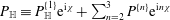 $P_{\mathbb{H}}\equiv P_{\mathbb{H}}^{\{1\}}\text{e}^{\text{i}\unicode[STIX]{x1D712}}+\sum _{n=2}^{3}P^{\{n\}}\text{e}^{\text{i}n\unicode[STIX]{x1D712}}$
and
$P_{\mathbb{H}}\equiv P_{\mathbb{H}}^{\{1\}}\text{e}^{\text{i}\unicode[STIX]{x1D712}}+\sum _{n=2}^{3}P^{\{n\}}\text{e}^{\text{i}n\unicode[STIX]{x1D712}}$
and
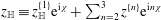 $z_{\mathbb{H}}\equiv z_{\mathbb{H}}^{\{1\}}\text{e}^{\text{i}\unicode[STIX]{x1D712}}+\sum _{n=2}^{3}z^{\{n\}}\text{e}^{\text{i}n\unicode[STIX]{x1D712}}$
, where
$z_{\mathbb{H}}\equiv z_{\mathbb{H}}^{\{1\}}\text{e}^{\text{i}\unicode[STIX]{x1D712}}+\sum _{n=2}^{3}z^{\{n\}}\text{e}^{\text{i}n\unicode[STIX]{x1D712}}$
, where
 $$\begin{eqnarray}\displaystyle & \displaystyle P_{\mathbb{H}}^{\{1\}}=C_{(2)}\text{e}^{k\unicode[STIX]{x1D701}}+\mathop{\sum }_{n\geqslant 1}C_{(n,3)}\cos \left(\sqrt{K_{(n)}^{2}-k^{2}}y+C_{(n,4)}\right)\text{e}^{K_{(n)}\unicode[STIX]{x1D701}}, & \displaystyle\end{eqnarray}$$
 $$\begin{eqnarray}\displaystyle & \displaystyle u_{\mathbb{H}}^{\{1\}}=\frac{\hat{k}_{1}}{c^{[0]}}P_{\mathbb{H}}^{\{1\}}-\frac{\text{i}\hat{k}_{1}}{g}\unicode[STIX]{x2202}_{t}^{\unicode[STIX]{x1D701}}P_{\mathbb{ H}}^{\{1\}}, & \displaystyle\end{eqnarray}$$
 $$\begin{eqnarray}\displaystyle & \displaystyle v_{\mathbb{H}}^{\{1\}}=-\frac{\text{i}}{c^{[0]}k}\unicode[STIX]{x2202}_{2}^{\unicode[STIX]{x1D701}}P_{\mathbb{H}}^{\{1\}}-\frac{1}{gk}\unicode[STIX]{x2202}_{2}^{\unicode[STIX]{x1D701}}\unicode[STIX]{x2202}_{t}^{\unicode[STIX]{x1D701}}P_{\mathbb{ H}}^{\{1\}}, & \displaystyle\end{eqnarray}$$
 $$\begin{eqnarray}\displaystyle & \displaystyle w_{\mathbb{H}}^{\{1\}}=-\frac{\text{i}}{c^{[0]}k}\unicode[STIX]{x2202}_{3}^{\unicode[STIX]{x1D701}}P_{\mathbb{H}}^{\{1\}}-\frac{1}{gk}\unicode[STIX]{x2202}_{3}^{\unicode[STIX]{x1D701}}\unicode[STIX]{x2202}_{t}^{\unicode[STIX]{x1D701}}P_{\mathbb{ H}}^{\{1\}}, & \displaystyle\end{eqnarray}$$
 $$\begin{eqnarray}\displaystyle & \displaystyle z_{\mathbb{H}}^{\{1\}}=\frac{1}{gk}\unicode[STIX]{x2202}_{3}^{\unicode[STIX]{x1D701}}P_{\mathbb{ H}}^{\{1\}}-\text{i}\frac{2}{gc^{[0]}k^{2}}\unicode[STIX]{x2202}_{3}^{\unicode[STIX]{x1D701}}\unicode[STIX]{x2202}_{t}^{\unicode[STIX]{x1D701}}P_{\mathbb{H}}^{\{1\}}. & \displaystyle\end{eqnarray}$$
 $P^{\{2\}}$
,
$P^{\{2\}}$
,
 $u_{i}^{\{2\}}$
,
$u_{i}^{\{2\}}$
,
 $z^{\{2\}}$
,
$z^{\{2\}}$
,
 $P^{\{3\}}$
,
$P^{\{3\}}$
,
 $u_{i}^{\{3\}}$
and
$u_{i}^{\{3\}}$
and
 $z^{\{3\}}$
are given by (D 4) and (D 5), and
$z^{\{3\}}$
are given by (D 4) and (D 5), and
 $C_{(2)}$
,
$C_{(2)}$
,
 $C_{(n,3)}$
,
$C_{(n,3)}$
,
 $C_{(n,4)}$
and
$C_{(n,4)}$
and
 $K_{(n)}$
are defined in § A.4. The
$K_{(n)}$
are defined in § A.4. The
 $\mathbb{H}$
-wave is the only wave type that contains the second and third harmonics. The
$\mathbb{H}$
-wave is the only wave type that contains the second and third harmonics. The
 $\mathbb{H}$
-wave satisfies
$\mathbb{H}$
-wave satisfies  $$\begin{eqnarray}\displaystyle & \displaystyle \unicode[STIX]{x1D735}\boldsymbol{\cdot }\boldsymbol{u}_{\mathbb{H}}=\unicode[STIX]{x2202}_{i}^{z}{u_{\mathbb{H}}}_{i}=O(\unicode[STIX]{x1D716}^{4}c^{[0]}k), & \displaystyle\end{eqnarray}$$
 $$\begin{eqnarray}\displaystyle & \displaystyle \unicode[STIX]{x2202}_{t}^{\unicode[STIX]{x1D701}}{u_{\mathbb{H}}}_{i}+\unicode[STIX]{x2202}_{i}^{\unicode[STIX]{x1D701}}P_{\mathbb{H}}=O(\unicode[STIX]{x1D716}^{4}{c^{[0]}}^{2}k). & \displaystyle\end{eqnarray}$$
Therefore, the
 $\mathbb{H}$
-wave is divergence-free to third order, and it is driven solely by the boundary conditions.
$\mathbb{H}$
-wave is divergence-free to third order, and it is driven solely by the boundary conditions.
5.2.2
$\mathbb{A}$
-wave

The
 $\mathbb{A}$
-wave occurs due to the coexistence of the leading-order wave
$\mathbb{A}$
-wave occurs due to the coexistence of the leading-order wave
 ${u_{i}^{w}}^{[1]}$
and the vertical shear of the along-roll jet
${u_{i}^{w}}^{[1]}$
and the vertical shear of the along-roll jet
 $\unicode[STIX]{x2202}_{3}^{\unicode[STIX]{x1D701}}u_{1}^{c}$
. Define the
$\unicode[STIX]{x2202}_{3}^{\unicode[STIX]{x1D701}}u_{1}^{c}$
. Define the
 $\mathbb{A}$
-wave as
$\mathbb{A}$
-wave as
 $u_{\mathbb{A}i}\equiv u_{\mathbb{A}i}^{\{1\}}\text{e}^{\text{i}\unicode[STIX]{x1D712}}$
,
$u_{\mathbb{A}i}\equiv u_{\mathbb{A}i}^{\{1\}}\text{e}^{\text{i}\unicode[STIX]{x1D712}}$
,
 $P_{\mathbb{A}}\equiv P_{\mathbb{A}}^{\{1\}}\text{e}^{\text{i}\unicode[STIX]{x1D712}}$
and
$P_{\mathbb{A}}\equiv P_{\mathbb{A}}^{\{1\}}\text{e}^{\text{i}\unicode[STIX]{x1D712}}$
and
 $z_{\mathbb{A}}\equiv z_{\mathbb{A}}^{\{1\}}\text{e}^{\text{i}\unicode[STIX]{x1D712}}$
, where
$z_{\mathbb{A}}\equiv z_{\mathbb{A}}^{\{1\}}\text{e}^{\text{i}\unicode[STIX]{x1D712}}$
, where
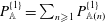 $P_{\mathbb{A}}^{\{1\}}=\sum _{n\geqslant 1}P_{\mathbb{A}(n)}^{\{1\}}$
and
$P_{\mathbb{A}}^{\{1\}}=\sum _{n\geqslant 1}P_{\mathbb{A}(n)}^{\{1\}}$
and
 $$\begin{eqnarray}\displaystyle P_{\mathbb{A}(n)}^{\{1\}} & = & \displaystyle \int _{\unicode[STIX]{x1D701}^{\prime }=\unicode[STIX]{x1D701}}^{0}\text{e}^{K_{\mathbb{A}(n)}(\unicode[STIX]{x1D701}-\unicode[STIX]{x1D701}^{\prime })}\frac{\mathbb{A}_{(n)}(x,y,\unicode[STIX]{x1D701}^{\prime },t)}{2K_{\mathbb{A}(n)}}\,\text{d}\unicode[STIX]{x1D701}^{\prime }\nonumber\\ \displaystyle & & \displaystyle +\,\int _{\unicode[STIX]{x1D701}^{\prime }=-\infty }^{\unicode[STIX]{x1D701}}\text{e}^{K_{\mathbb{A}(n)}(\unicode[STIX]{x1D701}^{\prime }-\unicode[STIX]{x1D701})}\frac{\mathbb{A}_{(n)}(x,y,\unicode[STIX]{x1D701}^{\prime },t)}{2K_{\mathbb{A}(n)}}\,\text{d}\unicode[STIX]{x1D701}^{\prime },\end{eqnarray}$$
 $$\begin{eqnarray}\displaystyle & \displaystyle u_{\mathbb{A}}^{\{1\}}=\frac{\hat{k}_{1}}{c^{[0]}}P_{\mathbb{A}}^{\{1\}}+\hat{k}_{1}ak\text{e}^{k\unicode[STIX]{x1D701}}\hat{k}_{1}(u_{1}^{c}-u_{1}^{D}), & \displaystyle\end{eqnarray}$$
 $$\begin{eqnarray}\displaystyle & \displaystyle v_{\mathbb{A}}^{\{1\}}=-\frac{\text{i}}{c^{[0]}k}\unicode[STIX]{x2202}_{2}^{\unicode[STIX]{x1D701}}P_{\mathbb{A}}^{\{1\}}, & \displaystyle\end{eqnarray}$$
 $$\begin{eqnarray}\displaystyle & \displaystyle w_{\mathbb{A}}^{\{1\}}=-\frac{\text{i}}{c^{[0]}k}\unicode[STIX]{x2202}_{3}^{\unicode[STIX]{x1D701}}P_{\mathbb{A}}^{\{1\}}-\text{i}ak\text{e}^{k\unicode[STIX]{x1D701}}\hat{k}_{1}(u_{1}^{c}-u_{1}^{D}), & \displaystyle\end{eqnarray}$$
 $$\begin{eqnarray}\displaystyle & \displaystyle z_{\mathbb{A}}^{\{1\}}=\frac{1}{gk}\unicode[STIX]{x2202}_{3}^{\unicode[STIX]{x1D701}}P_{\mathbb{ A}}^{\{1\}}+\frac{2a}{c^{[0]}}\text{e}^{k\unicode[STIX]{x1D701}}\hat{k}_{1}(u_{1}^{c}-u_{1}^{D}). & \displaystyle\end{eqnarray}$$
 $u_{1}^{D}$
is given by (5.15a
), and
$u_{1}^{D}$
is given by (5.15a
), and
 $\mathbb{A}_{(n)}$
and
$\mathbb{A}_{(n)}$
and
 $K_{\mathbb{A}(n)}$
are given in table 1. The
$K_{\mathbb{A}(n)}$
are given in table 1. The
 $\mathbb{A}$
-wave is divergent and cancels the undulation-induced divergence of the current shown in (4.1) and figure 3(a), namely,
$\mathbb{A}$
-wave is divergent and cancels the undulation-induced divergence of the current shown in (4.1) and figure 3(a), namely,  $$\begin{eqnarray}\unicode[STIX]{x2202}_{i}^{z}{u_{\mathbb{ A}}}_{i}-S_{h}^{[1]}\unicode[STIX]{x2202}_{3}^{\unicode[STIX]{x1D701}}u_{h}^{c}=O(\unicode[STIX]{x1D716}^{4}c^{[0]}k).\end{eqnarray}$$
The
 $\mathbb{A}$
-wave satisfies the momentum balance as
$\mathbb{A}$
-wave satisfies the momentum balance as
 $$\begin{eqnarray}\unicode[STIX]{x2202}_{t}^{\unicode[STIX]{x1D701}}{u_{\mathbb{ A}}}_{i}+\unicode[STIX]{x2202}_{i}^{\unicode[STIX]{x1D701}}P_{\mathbb{ A}}+F_{\mathbb{A}i}=O(\unicode[STIX]{x1D716}^{4}{c^{[0]}}^{2}k).\end{eqnarray}$$
Note that
 $u_{h}^{c}-u_{h}^{D}$
in (5.17) represents the vertically sheared part of the horizontal current. Therefore,
$u_{h}^{c}-u_{h}^{D}$
in (5.17) represents the vertically sheared part of the horizontal current. Therefore,
 $F_{\mathbb{A}i}$
is the advection of the leading-order wave velocities
$F_{\mathbb{A}i}$
is the advection of the leading-order wave velocities
 ${u_{i}^{w}}^{[1]}$
by the vertically sheared part of the horizontal current. Figure 5 shows the velocities of the
${u_{i}^{w}}^{[1]}$
by the vertically sheared part of the horizontal current. Figure 5 shows the velocities of the
 $\mathbb{A}$
-wave due to the current shown in figure 2 and the leading-order wave having
$\mathbb{A}$
-wave due to the current shown in figure 2 and the leading-order wave having
 $(\hat{k}_{1},\hat{k}_{2})=(1,0)$
. Note that
$(\hat{k}_{1},\hat{k}_{2})=(1,0)$
. Note that
 $u_{\mathbb{A}}$
is in phase with
$u_{\mathbb{A}}$
is in phase with
 $\unicode[STIX]{x2202}_{1}^{\unicode[STIX]{x1D701}}{w^{w}}^{[1]}$
. This correlation is crucial because it converts the oscillatory motion
$\unicode[STIX]{x2202}_{1}^{\unicode[STIX]{x1D701}}{w^{w}}^{[1]}$
. This correlation is crucial because it converts the oscillatory motion
 ${w^{w}}^{[1]}$
into a non-oscillatory vertical motion via the advection
${w^{w}}^{[1]}$
into a non-oscillatory vertical motion via the advection
 $u_{\mathbb{A}}\unicode[STIX]{x2202}_{1}^{\unicode[STIX]{x1D701}}{w^{w}}^{[1]}$
at the fourth-order balance. The
$u_{\mathbb{A}}\unicode[STIX]{x2202}_{1}^{\unicode[STIX]{x1D701}}{w^{w}}^{[1]}$
at the fourth-order balance. The
 $\mathbb{A}$
-wave is divergent at the places corresponding to contours 2 and 4 of figure 3(a) to cancel the undulation-induced divergence of the current. The
$\mathbb{A}$
-wave is divergent at the places corresponding to contours 2 and 4 of figure 3(a) to cancel the undulation-induced divergence of the current. The
 $\mathbb{A}$
-wave ceases towards the upwelling section because the vertical shear of
$\mathbb{A}$
-wave ceases towards the upwelling section because the vertical shear of
 $u_{1}^{c}$
ceases towards the upwelling section in this example (figure 2). We have that
$u_{1}^{c}$
ceases towards the upwelling section in this example (figure 2). We have that
 $w_{\mathbb{A}}$
is negligible because the first and second terms on the right-hand side of (5.26d
) largely cancel each other. On the other hand,
$w_{\mathbb{A}}$
is negligible because the first and second terms on the right-hand side of (5.26d
) largely cancel each other. On the other hand,
 $u_{\mathbb{A}}$
is approximately twice as large as each term on the right-hand side of (5.26b
) because the two terms on the right-hand side of (5.26b
) are similar to each other. The profile of
$u_{\mathbb{A}}$
is approximately twice as large as each term on the right-hand side of (5.26b
) because the two terms on the right-hand side of (5.26b
) are similar to each other. The profile of
 $u_{1}^{c}$
in this example and the corresponding
$u_{1}^{c}$
in this example and the corresponding
 $u_{1}^{D}$
computed from (5.15a
) are shown in figure 6.
$u_{1}^{D}$
computed from (5.15a
) are shown in figure 6.

Figure 5. The
 $\mathbb{A}$
-wave at the downwelling section (
$\mathbb{A}$
-wave at the downwelling section (
 $ky=0$
), at the middle section (
$ky=0$
), at the middle section (
 $ky=0.9\unicode[STIX]{x03C0}$
) and at the upwelling section (
$ky=0.9\unicode[STIX]{x03C0}$
) and at the upwelling section (
 $ky=1.8\unicode[STIX]{x03C0}$
) shown in figure 2. The colour shows
$ky=1.8\unicode[STIX]{x03C0}$
) shown in figure 2. The colour shows
 $u_{\mathbb{A}i}/(\unicode[STIX]{x1D716}^{3}c^{[0]})$
.
$u_{\mathbb{A}i}/(\unicode[STIX]{x1D716}^{3}c^{[0]})$
.

Figure 6. Plots of
 $u_{1}^{c}$
(solid) and
$u_{1}^{c}$
(solid) and
 $u_{1}^{D}$
(dashed) at the downwelling section (
$u_{1}^{D}$
(dashed) at the downwelling section (
 $ky=0$
), at the middle section (
$ky=0$
), at the middle section (
 $ky=0.9\unicode[STIX]{x03C0}$
) and at the upwelling section (
$ky=0.9\unicode[STIX]{x03C0}$
) and at the upwelling section (
 $ky=1.8\unicode[STIX]{x03C0}$
) in figure 2. The velocities in (c) are zero.
$ky=1.8\unicode[STIX]{x03C0}$
) in figure 2. The velocities in (c) are zero.

Figure 7. The
 $\mathbb{B}$
-wave at the downwelling section (
$\mathbb{B}$
-wave at the downwelling section (
 $ky=0$
), at the middle section (
$ky=0$
), at the middle section (
 $ky=0.9\unicode[STIX]{x03C0}$
) and at the upwelling section (
$ky=0.9\unicode[STIX]{x03C0}$
) and at the upwelling section (
 $ky=1.8\unicode[STIX]{x03C0}$
) shown in figure 2. The colour shows
$ky=1.8\unicode[STIX]{x03C0}$
) shown in figure 2. The colour shows
 $u_{\mathbb{B}i}/(\unicode[STIX]{x1D716}^{3}c^{[0]})$
.
$u_{\mathbb{B}i}/(\unicode[STIX]{x1D716}^{3}c^{[0]})$
.
5.2.3
$\mathbb{B}$
-wave

The
 $\mathbb{B}$
-wave occurs due to the coexistence of the leading-order wave and the roll. Define the
$\mathbb{B}$
-wave occurs due to the coexistence of the leading-order wave and the roll. Define the
 $\mathbb{B}$
-wave as
$\mathbb{B}$
-wave as
 $u_{\mathbb{B}i}\equiv u_{\mathbb{B}i}^{\{1\}}\text{e}^{\text{i}\unicode[STIX]{x1D712}}$
,
$u_{\mathbb{B}i}\equiv u_{\mathbb{B}i}^{\{1\}}\text{e}^{\text{i}\unicode[STIX]{x1D712}}$
,
 $P_{\mathbb{B}}\equiv P_{\mathbb{B}}^{\{1\}}\text{e}^{\text{i}\unicode[STIX]{x1D712}}$
and
$P_{\mathbb{B}}\equiv P_{\mathbb{B}}^{\{1\}}\text{e}^{\text{i}\unicode[STIX]{x1D712}}$
and
 $z_{\mathbb{B}}\equiv z_{\mathbb{B}}^{\{1\}}\text{e}^{\text{i}\unicode[STIX]{x1D712}}$
, where
$z_{\mathbb{B}}\equiv z_{\mathbb{B}}^{\{1\}}\text{e}^{\text{i}\unicode[STIX]{x1D712}}$
, where
 $P_{\mathbb{B}}^{\{1\}}=\sum _{n\geqslant 1}P_{\mathbb{B}(n)}^{\{1\}}$
and
$P_{\mathbb{B}}^{\{1\}}=\sum _{n\geqslant 1}P_{\mathbb{B}(n)}^{\{1\}}$
and
 $$\begin{eqnarray}\displaystyle P_{\mathbb{B}(n)}^{\{1\}} & = & \displaystyle \int _{\unicode[STIX]{x1D701}^{\prime }=\unicode[STIX]{x1D701}}^{0}\text{e}^{K_{\mathbb{B}(n)}(\unicode[STIX]{x1D701}-\unicode[STIX]{x1D701}^{\prime })}\frac{\mathbb{B}_{(n)}(x,y,\unicode[STIX]{x1D701}^{\prime },t)}{2K_{\mathbb{B}(n)}}\,\text{d}\unicode[STIX]{x1D701}^{\prime }\nonumber\\ \displaystyle & & \displaystyle +\,\int _{\unicode[STIX]{x1D701}^{\prime }=-\infty }^{\unicode[STIX]{x1D701}}\text{e}^{K_{\mathbb{B}(n)}(\unicode[STIX]{x1D701}^{\prime }-\unicode[STIX]{x1D701})}\frac{\mathbb{B}_{(n)}(x,y,\unicode[STIX]{x1D701}^{\prime },t)}{2K_{\mathbb{B}(n)}}\,\text{d}\unicode[STIX]{x1D701}^{\prime },\end{eqnarray}$$
 $$\begin{eqnarray}\displaystyle & \displaystyle u_{\mathbb{B}}^{\{1\}}=\frac{\hat{k}_{1}}{c^{[0]}}P_{\mathbb{B}}^{\{1\}}-\text{i}\hat{k}_{1}ak\text{e}^{k\unicode[STIX]{x1D701}}w^{c}, & \displaystyle\end{eqnarray}$$
 $$\begin{eqnarray}\displaystyle & \displaystyle v_{\mathbb{B}}^{\{1\}}=-\frac{\text{i}}{c^{[0]}k}\unicode[STIX]{x2202}_{2}^{\unicode[STIX]{x1D701}}P_{\mathbb{B}}^{\{1\}}, & \displaystyle\end{eqnarray}$$
 $$\begin{eqnarray}\displaystyle & \displaystyle w_{\mathbb{B}}^{\{1\}}=-\frac{\text{i}}{c^{[0]}k}\unicode[STIX]{x2202}_{3}^{\unicode[STIX]{x1D701}}P_{\mathbb{B}}^{\{1\}}-ak\text{e}^{k\unicode[STIX]{x1D701}}w^{c}, & \displaystyle\end{eqnarray}$$
 $$\begin{eqnarray}\displaystyle & \displaystyle z_{\mathbb{B}}^{\{1\}}=\frac{1}{gk}\unicode[STIX]{x2202}_{3}^{\unicode[STIX]{x1D701}}P_{\mathbb{ B}}^{\{1\}}-\text{i}\frac{a}{c^{[0]}}\text{e}^{k\unicode[STIX]{x1D701}}w^{c}. & \displaystyle\end{eqnarray}$$
 $\mathbb{B}_{(n)}$
and
$\mathbb{B}_{(n)}$
and
 $K_{\mathbb{B}(n)}$
are given in table 1. The
$K_{\mathbb{B}(n)}$
are given in table 1. The
 $\mathbb{B}$
-wave exists to cancel the undulation-induced divergence of the current due to
$\mathbb{B}$
-wave exists to cancel the undulation-induced divergence of the current due to
 $\unicode[STIX]{x2202}_{3}^{\unicode[STIX]{x1D701}}w^{c}$
and
$\unicode[STIX]{x2202}_{3}^{\unicode[STIX]{x1D701}}w^{c}$
and
 $S_{3}$
shown in (4.1) and figure 3(b), namely,
$S_{3}$
shown in (4.1) and figure 3(b), namely,  $$\begin{eqnarray}\unicode[STIX]{x2202}_{i}^{z}{u_{\mathbb{ B}}}_{i}-S_{3}^{[1]}\unicode[STIX]{x2202}_{3}^{\unicode[STIX]{x1D701}}w^{c}=O(\unicode[STIX]{x1D716}^{4}c^{[0]}k).\end{eqnarray}$$
Therefore, according to (4.1), (5.27) and (5.30), the
 $\mathbb{A}$
- and
$\mathbb{A}$
- and
 $\mathbb{B}$
-waves cancel the current divergence to third order:
$\mathbb{B}$
-waves cancel the current divergence to third order:
 $\unicode[STIX]{x1D735}\boldsymbol{\cdot }(\boldsymbol{u}^{c}+\boldsymbol{u}_{\mathbb{A}}+\boldsymbol{u}_{\mathbb{B}})=O(\unicode[STIX]{x1D716}^{4}c^{[0]}k)$
. The
$\unicode[STIX]{x1D735}\boldsymbol{\cdot }(\boldsymbol{u}^{c}+\boldsymbol{u}_{\mathbb{A}}+\boldsymbol{u}_{\mathbb{B}})=O(\unicode[STIX]{x1D716}^{4}c^{[0]}k)$
. The
 $\mathbb{B}$
-wave satisfies
$\mathbb{B}$
-wave satisfies
 $$\begin{eqnarray}\unicode[STIX]{x2202}_{t}^{\unicode[STIX]{x1D701}}{u_{\mathbb{ B}}}_{i}+\unicode[STIX]{x2202}_{i}^{\unicode[STIX]{x1D701}}P_{\mathbb{ B}}+F_{\mathbb{B}i}=O(\unicode[STIX]{x1D716}^{4}{c^{[0]}}^{2}k).\end{eqnarray}$$
The
 $F_{\mathbb{B}i}$
defined in (5.18) is the vertical advection of the leading-order wave momentum by the vertical current. Figure 7 shows the velocities of the
$F_{\mathbb{B}i}$
defined in (5.18) is the vertical advection of the leading-order wave momentum by the vertical current. Figure 7 shows the velocities of the
 $\mathbb{B}$
-wave due to the current shown in figure 2 and the leading-order wave having
$\mathbb{B}$
-wave due to the current shown in figure 2 and the leading-order wave having
 $(\hat{k}_{1},\hat{k}_{2})=(1,0)$
. The
$(\hat{k}_{1},\hat{k}_{2})=(1,0)$
. The
 $\mathbb{B}$
-wave is divergent at the places corresponding to contours 1 and 3 of figure 3(b). Unlike the
$\mathbb{B}$
-wave is divergent at the places corresponding to contours 1 and 3 of figure 3(b). Unlike the
 $\mathbb{A}$
-wave, the
$\mathbb{A}$
-wave, the
 $\mathbb{B}$
-wave has significant
$\mathbb{B}$
-wave has significant
 $v_{\mathbb{B}}$
and
$v_{\mathbb{B}}$
and
 $w_{\mathbb{B}}$
.
$w_{\mathbb{B}}$
.
5.2.4
$\mathbb{C}$
-wave

The
 $\mathbb{C}$
-wave exists for the same reason as the
$\mathbb{C}$
-wave exists for the same reason as the
 $\mathbb{A}$
-wave except that the relevant flow is
$\mathbb{A}$
-wave except that the relevant flow is
 $u_{1}^{c}$
for the
$u_{1}^{c}$
for the
 $\mathbb{A}$
-wave and
$\mathbb{A}$
-wave and
 $\mathfrak{U}_{1}$
for the
$\mathfrak{U}_{1}$
for the
 $\mathbb{C}$
-wave. Define the
$\mathbb{C}$
-wave. Define the
 $\mathbb{C}$
-wave as
$\mathbb{C}$
-wave as
 $u_{\mathbb{C}i}\equiv u_{\mathbb{C}i}^{\{1\}}\text{e}^{\text{i}\unicode[STIX]{x1D712}}$
,
$u_{\mathbb{C}i}\equiv u_{\mathbb{C}i}^{\{1\}}\text{e}^{\text{i}\unicode[STIX]{x1D712}}$
,
 $P_{\mathbb{C}}\equiv P_{\mathbb{C}}^{\{1\}}\text{e}^{\text{i}\unicode[STIX]{x1D712}}$
and
$P_{\mathbb{C}}\equiv P_{\mathbb{C}}^{\{1\}}\text{e}^{\text{i}\unicode[STIX]{x1D712}}$
and
 $z_{\mathbb{C}}\equiv z_{\mathbb{C}}^{\{1\}}\text{e}^{\text{i}\unicode[STIX]{x1D712}}$
, where
$z_{\mathbb{C}}\equiv z_{\mathbb{C}}^{\{1\}}\text{e}^{\text{i}\unicode[STIX]{x1D712}}$
, where
 $$\begin{eqnarray}\displaystyle & \displaystyle P_{\mathbb{C}}^{\{1\}}=\int _{\unicode[STIX]{x1D701}^{\prime }=\unicode[STIX]{x1D701}}^{0}\text{e}^{k(\unicode[STIX]{x1D701}-\unicode[STIX]{x1D701}^{\prime })}\frac{\mathbb{C}(x,y,\unicode[STIX]{x1D701}^{\prime },t)}{2k}\,\text{d}\unicode[STIX]{x1D701}^{\prime }+\int _{\unicode[STIX]{x1D701}^{\prime }=-\infty }^{\unicode[STIX]{x1D701}}\text{e}^{k(\unicode[STIX]{x1D701}^{\prime }-\unicode[STIX]{x1D701})}\frac{\mathbb{C}(x,y,\unicode[STIX]{x1D701}^{\prime },t)}{2k}\,\text{d}\unicode[STIX]{x1D701}^{\prime },\quad & \displaystyle\end{eqnarray}$$
 $$\begin{eqnarray}\displaystyle & \displaystyle u_{\mathbb{C}}^{\{1\}}=\frac{\hat{k}_{1}}{c^{[0]}}P_{\mathbb{C}}^{\{1\}}+\hat{k}_{1}ak\text{e}^{k\unicode[STIX]{x1D701}}\left(\hat{k}_{1}\mathfrak{U}_{1}-c^{[2]}+\frac{1}{2}c^{[0]}a^{2}k^{2}\text{e}^{2k\unicode[STIX]{x1D701}}\right)+\text{i}\hat{k}_{1}\frac{a}{c^{[0]}}\text{e}^{k\unicode[STIX]{x1D701}}\unicode[STIX]{x2202}_{t}c^{[2]},\quad & \displaystyle\end{eqnarray}$$
 $$\begin{eqnarray}\displaystyle & \displaystyle v_{\mathbb{C}}^{\{1\}}=-\frac{\text{i}}{c^{[0]}k}\unicode[STIX]{x2202}_{2}^{\unicode[STIX]{x1D701}}P_{\mathbb{C}}^{\{1\}}, & \displaystyle\end{eqnarray}$$
 $$\begin{eqnarray}\displaystyle & \displaystyle w_{\mathbb{C}}^{\{1\}}=-\frac{\text{i}}{c^{[0]}k}\unicode[STIX]{x2202}_{3}^{\unicode[STIX]{x1D701}}P_{\mathbb{C}}^{\{1\}}-\text{i}ak\text{e}^{k\unicode[STIX]{x1D701}}\left(\hat{k}_{1}\mathfrak{U}_{1}-c^{[2]}+\frac{1}{2}c^{[0]}a^{2}k^{2}\text{e}^{2k\unicode[STIX]{x1D701}}\right)+\frac{a}{c^{[0]}}\text{e}^{k\unicode[STIX]{x1D701}}\unicode[STIX]{x2202}_{t}c^{[2]},\quad & \displaystyle\end{eqnarray}$$
 $$\begin{eqnarray}\displaystyle & \displaystyle z_{\mathbb{C}}^{\{1\}}=\frac{1}{gk}\unicode[STIX]{x2202}_{3}^{\unicode[STIX]{x1D701}}P_{\mathbb{ C}}^{\{1\}}+\frac{2a}{c^{[0]}}\text{e}^{k\unicode[STIX]{x1D701}}\left(\hat{k}_{1}\mathfrak{U}_{1}-c^{[2]}+\frac{3}{8}c^{[0]}a^{2}k^{2}\text{e}^{2k\unicode[STIX]{x1D701}}\right)+\text{i}\frac{3a}{g}\text{e}^{k\unicode[STIX]{x1D701}}\unicode[STIX]{x2202}_{t}c^{[2]}. & \displaystyle\end{eqnarray}$$
 $\mathbb{C}$
is defined in table 1, and
$\mathbb{C}$
is defined in table 1, and
 $c^{[2]}$
and
$c^{[2]}$
and
 $\unicode[STIX]{x2202}_{t}c^{[2]}$
are given by (5.15b
) and (D 3b
). The
$\unicode[STIX]{x2202}_{t}c^{[2]}$
are given by (5.15b
) and (D 3b
). The
 $\mathbb{C}$
-wave is divergent and cancels the undulation-induced divergence of
$\mathbb{C}$
-wave is divergent and cancels the undulation-induced divergence of
 $\mathfrak{U}_{h}$
, namely,
$\mathfrak{U}_{h}$
, namely,  $$\begin{eqnarray}\unicode[STIX]{x2202}_{i}^{z}u_{\mathbb{ C}i}-S_{h}^{[1]}\unicode[STIX]{x2202}_{3}^{\unicode[STIX]{x1D701}}\mathfrak{U}_{h}=O(\unicode[STIX]{x1D716}^{4}c^{[0]}k).\end{eqnarray}$$
Then, because
 $\unicode[STIX]{x2202}_{i}^{z}\mathfrak{U}_{i}=-S_{h}^{[1]}\unicode[STIX]{x2202}_{3}^{\unicode[STIX]{x1D701}}\mathfrak{U}_{h}+O(\unicode[STIX]{x1D716}^{4}c^{[0]}k)$
according to the chain rule (2.15) and the scaling conditions in § 3, the
$\unicode[STIX]{x2202}_{i}^{z}\mathfrak{U}_{i}=-S_{h}^{[1]}\unicode[STIX]{x2202}_{3}^{\unicode[STIX]{x1D701}}\mathfrak{U}_{h}+O(\unicode[STIX]{x1D716}^{4}c^{[0]}k)$
according to the chain rule (2.15) and the scaling conditions in § 3, the
 $\mathbb{C}$
-wave cancels the divergence of
$\mathbb{C}$
-wave cancels the divergence of
 $\mathfrak{U}_{i}$
to third order: that is,
$\mathfrak{U}_{i}$
to third order: that is,
 $\unicode[STIX]{x2202}_{i}^{z}(u_{\mathbb{C}i}+\mathfrak{U}_{i})=O(\unicode[STIX]{x1D716}^{4}c^{[0]}k)$
. The
$\unicode[STIX]{x2202}_{i}^{z}(u_{\mathbb{C}i}+\mathfrak{U}_{i})=O(\unicode[STIX]{x1D716}^{4}c^{[0]}k)$
. The
 $\mathbb{C}$
-wave is driven by
$\mathbb{C}$
-wave is driven by
 $F_{\mathbb{C}i}$
as
$F_{\mathbb{C}i}$
as
 $$\begin{eqnarray}\unicode[STIX]{x2202}_{t}^{\unicode[STIX]{x1D701}}{u_{\mathbb{ C}}}_{i}+\unicode[STIX]{x2202}_{i}^{\unicode[STIX]{x1D701}}P_{\mathbb{ C}}+F_{\mathbb{C}i}=O(\unicode[STIX]{x1D716}^{4}{c^{[0]}}^{2}k).\end{eqnarray}$$
According to the first- and second-order wave solutions (5.7) and (5.9) as well as the scaling conditions in § 3, the term surrounded by the square brackets in (5.19) satisfies
 $$\begin{eqnarray}[u_{h}^{w}\unicode[STIX]{x2202}_{h}^{\unicode[STIX]{x1D701}}u_{i}^{w}-S_{i}J^{-1}\unicode[STIX]{x2202}_{3}^{\unicode[STIX]{x1D701}}P]=(\mathfrak{U}_{h}+{\textstyle \frac{1}{2}}c^{[0]}a^{2}k^{2}\text{e}^{2k\unicode[STIX]{x1D701}}\hat{k}_{h})\unicode[STIX]{x2202}_{h}^{\unicode[STIX]{x1D701}}{u_{i}^{w}}^{[1]}+O(\unicode[STIX]{x1D716}^{4}{c^{[0]}}^{2}k).\end{eqnarray}$$
Therefore,
 $F_{\mathbb{C}i}$
is analogous to
$F_{\mathbb{C}i}$
is analogous to
 $F_{\mathbb{A}i}$
, with
$F_{\mathbb{A}i}$
, with
 $u_{h}^{c}$
corresponding to
$u_{h}^{c}$
corresponding to
 $\mathfrak{U}_{h}+(1/2)c^{[0]}a^{2}k^{2}\text{e}^{2k\unicode[STIX]{x1D701}}\hat{k}_{h}$
and
$\mathfrak{U}_{h}+(1/2)c^{[0]}a^{2}k^{2}\text{e}^{2k\unicode[STIX]{x1D701}}\hat{k}_{h}$
and
 $u_{h}^{D}$
corresponding to
$u_{h}^{D}$
corresponding to
 $c^{[2]}\hat{k}_{h}$
.
$c^{[2]}\hat{k}_{h}$
.
5.2.5
$\mathbb{D}$
-wave

The
 $\mathbb{D}$
-wave exists due to the divergence of the
$\mathbb{D}$
-wave exists due to the divergence of the
 $\unicode[STIX]{x1D6E9}$
-dependent motions of the lower-order waves (i.e.
$\unicode[STIX]{x1D6E9}$
-dependent motions of the lower-order waves (i.e.
 ${u_{i}^{w}}^{[1]}+{u_{i}^{w}}^{[2]}-\mathfrak{U}_{i}$
). This divergence becomes non-zero to third order when the wave properties (
${u_{i}^{w}}^{[1]}+{u_{i}^{w}}^{[2]}-\mathfrak{U}_{i}$
). This divergence becomes non-zero to third order when the wave properties (
 $a$
,
$a$
,
 $k$
,
$k$
,
 $\hat{k}_{h}$
) vary. Define the
$\hat{k}_{h}$
) vary. Define the
 $\mathbb{D}$
-wave as
$\mathbb{D}$
-wave as
 $u_{\mathbb{D}i}\equiv u_{\mathbb{D}i}^{\{1\}}\text{e}^{\text{i}\unicode[STIX]{x1D712}}$
,
$u_{\mathbb{D}i}\equiv u_{\mathbb{D}i}^{\{1\}}\text{e}^{\text{i}\unicode[STIX]{x1D712}}$
,
 $P_{\mathbb{D}}\equiv P_{\mathbb{D}}^{\{1\}}\text{e}^{\text{i}\unicode[STIX]{x1D712}}$
and
$P_{\mathbb{D}}\equiv P_{\mathbb{D}}^{\{1\}}\text{e}^{\text{i}\unicode[STIX]{x1D712}}$
and
 $z_{\mathbb{D}}\equiv z_{\mathbb{D}}^{\{1\}}\text{e}^{\text{i}\unicode[STIX]{x1D712}}$
, where
$z_{\mathbb{D}}\equiv z_{\mathbb{D}}^{\{1\}}\text{e}^{\text{i}\unicode[STIX]{x1D712}}$
, where
 $$\begin{eqnarray}\displaystyle & \displaystyle P_{\mathbb{D}}^{\{1\}}=\unicode[STIX]{x1D6FC}_{\mathbb{D}}\unicode[STIX]{x1D701}^{2}\text{e}^{k\unicode[STIX]{x1D701}}+\unicode[STIX]{x1D6FD}_{\mathbb{D}}\unicode[STIX]{x1D701}\text{e}^{k\unicode[STIX]{x1D701}}+\unicode[STIX]{x1D6FE}_{\mathbb{D}}\text{e}^{k\unicode[STIX]{x1D701}}, & \displaystyle\end{eqnarray}$$
 $$\begin{eqnarray}\displaystyle & \displaystyle u_{\mathbb{D}}^{\{1\}}=\frac{\hat{k}_{1}}{c^{[0]}}P_{\mathbb{D}}^{\{1\}}-\frac{\text{i}\hat{k}_{1}}{g}\unicode[STIX]{x2202}_{t}^{\unicode[STIX]{x1D701}}P_{\mathbb{ D}}^{\{1\}}-\text{i}a\text{e}^{k\unicode[STIX]{x1D701}}\unicode[STIX]{x2202}_{t}\hat{k}_{1}-\text{i}c^{[0]}\unicode[STIX]{x2202}_{1}^{\unicode[STIX]{x1D701}}(a\text{e}^{k\unicode[STIX]{x1D701}}), & \displaystyle\end{eqnarray}$$
 $$\begin{eqnarray}\displaystyle & \displaystyle v_{\mathbb{D}}^{\{1\}}=-\frac{\text{i}}{c^{[0]}k}\unicode[STIX]{x2202}_{2}^{\unicode[STIX]{x1D701}}P_{\mathbb{D}}^{\{1\}}-\frac{1}{gk}\unicode[STIX]{x2202}_{2}^{\unicode[STIX]{x1D701}}\unicode[STIX]{x2202}_{t}^{\unicode[STIX]{x1D701}}P_{\mathbb{ D}}^{\{1\}}-\text{i}a\text{e}^{k\unicode[STIX]{x1D701}}\unicode[STIX]{x2202}_{t}\hat{k}_{2}-\frac{a}{c^{[0]}k}\text{e}^{k\unicode[STIX]{x1D701}}\unicode[STIX]{x2202}_{t}\unicode[STIX]{x2202}_{t}\hat{k}_{2}, & \displaystyle\end{eqnarray}$$
 $$\begin{eqnarray}\displaystyle & \displaystyle w_{\mathbb{D}}^{\{1\}}=-\frac{\text{i}}{c^{[0]}k}\unicode[STIX]{x2202}_{3}^{\unicode[STIX]{x1D701}}P_{\mathbb{D}}^{\{1\}}-\frac{1}{gk}\unicode[STIX]{x2202}_{3}^{\unicode[STIX]{x1D701}}\unicode[STIX]{x2202}_{t}^{\unicode[STIX]{x1D701}}P_{\mathbb{ D}}^{\{1\}}, & \displaystyle\end{eqnarray}$$
 $$\begin{eqnarray}\displaystyle & \displaystyle z_{\mathbb{D}}^{\{1\}}=\frac{1}{gk}\unicode[STIX]{x2202}_{3}^{\unicode[STIX]{x1D701}}P_{\mathbb{ D}}^{\{1\}}-\text{i}\frac{2}{gc^{[0]}k^{2}}\unicode[STIX]{x2202}_{3}^{\unicode[STIX]{x1D701}}\unicode[STIX]{x2202}_{t}^{\unicode[STIX]{x1D701}}P_{\mathbb{D}}^{\{1\}}. & \displaystyle\end{eqnarray}$$
 $\unicode[STIX]{x1D6FC}_{\mathbb{D}}$
,
$\unicode[STIX]{x1D6FC}_{\mathbb{D}}$
,
 $\unicode[STIX]{x1D6FD}_{\mathbb{D}}$
and
$\unicode[STIX]{x1D6FD}_{\mathbb{D}}$
and
 $\unicode[STIX]{x1D6FE}_{\mathbb{D}}$
are defined in table 1;
$\unicode[STIX]{x1D6FE}_{\mathbb{D}}$
are defined in table 1;
 $\unicode[STIX]{x2202}_{t}\hat{k}_{1}$
,
$\unicode[STIX]{x2202}_{t}\hat{k}_{1}$
,
 $\unicode[STIX]{x2202}_{t}\hat{k}_{2}$
and
$\unicode[STIX]{x2202}_{t}\hat{k}_{2}$
and
 $\unicode[STIX]{x2202}_{t}\unicode[STIX]{x2202}_{t}\hat{k}_{2}$
are given by (D 3c
), (C 5) and (D 3d
); and
$\unicode[STIX]{x2202}_{t}\unicode[STIX]{x2202}_{t}\hat{k}_{2}$
are given by (D 3c
), (C 5) and (D 3d
); and
 $\unicode[STIX]{x2202}_{t}^{\unicode[STIX]{x1D701}}P_{\mathbb{D}}^{\{1\}}$
to third order is given by (5.36a
) and (C 5). The
$\unicode[STIX]{x2202}_{t}^{\unicode[STIX]{x1D701}}P_{\mathbb{D}}^{\{1\}}$
to third order is given by (5.36a
) and (C 5). The
 $\mathbb{D}$
-wave satisfies
$\mathbb{D}$
-wave satisfies  $$\begin{eqnarray}\displaystyle & \displaystyle \unicode[STIX]{x2202}_{i}^{z}({u_{\mathbb{D}}}_{i}+{u_{i}^{w}}^{[1]}+{u_{i}^{w}}^{[2]}-\mathfrak{U}_{i})=O(\unicode[STIX]{x1D716}^{4}c^{[0]}k), & \displaystyle\end{eqnarray}$$
 $$\begin{eqnarray}\displaystyle & \displaystyle \unicode[STIX]{x2202}_{t}^{\unicode[STIX]{x1D701}}{u_{\mathbb{D}}}_{i}+\unicode[STIX]{x2202}_{i}^{\unicode[STIX]{x1D701}}P_{\mathbb{D}}+F_{\mathbb{D}i}=O(\unicode[STIX]{x1D716}^{4}{c^{[0]}}^{2}k). & \displaystyle\end{eqnarray}$$
Therefore, the
 $\mathbb{D}$
-wave cancels the divergence of the lower-order
$\mathbb{D}$
-wave cancels the divergence of the lower-order
 $\unicode[STIX]{x1D6E9}$
-dependent motions, and it is forced by the imbalance
$\unicode[STIX]{x1D6E9}$
-dependent motions, and it is forced by the imbalance
 $F_{\mathbb{D}i}$
due to a non-zero
$F_{\mathbb{D}i}$
due to a non-zero
 $\unicode[STIX]{x2202}_{t}\hat{k}_{h}$
,
$\unicode[STIX]{x2202}_{t}\hat{k}_{h}$
,
 $\unicode[STIX]{x2202}_{1}a$
or
$\unicode[STIX]{x2202}_{1}a$
or
 $\unicode[STIX]{x2202}_{1}k$
in (5.20).
$\unicode[STIX]{x2202}_{1}k$
in (5.20).
5.2.6
$\mathbb{E}$
-wave

The
 $\mathbb{E}$
-wave exists due to a non-zero
$\mathbb{E}$
-wave exists due to a non-zero
 $\unicode[STIX]{x2202}_{2}a$
or
$\unicode[STIX]{x2202}_{2}a$
or
 $\unicode[STIX]{x2202}_{2}k$
. Define the
$\unicode[STIX]{x2202}_{2}k$
. Define the
 $\mathbb{E}$
-wave as
$\mathbb{E}$
-wave as
 $u_{\mathbb{E}i}\equiv u_{\mathbb{E}i}^{\{1\}}\text{e}^{\text{i}\unicode[STIX]{x1D712}}$
,
$u_{\mathbb{E}i}\equiv u_{\mathbb{E}i}^{\{1\}}\text{e}^{\text{i}\unicode[STIX]{x1D712}}$
,
 $P_{\mathbb{E}}\equiv P_{\mathbb{E}}^{\{1\}}\text{e}^{\text{i}\unicode[STIX]{x1D712}}$
and
$P_{\mathbb{E}}\equiv P_{\mathbb{E}}^{\{1\}}\text{e}^{\text{i}\unicode[STIX]{x1D712}}$
and
 $z_{\mathbb{E}}\equiv z_{\mathbb{E}}^{\{1\}}\text{e}^{\text{i}\unicode[STIX]{x1D712}}$
, where
$z_{\mathbb{E}}\equiv z_{\mathbb{E}}^{\{1\}}\text{e}^{\text{i}\unicode[STIX]{x1D712}}$
, where
 $$\begin{eqnarray}\displaystyle & \displaystyle P_{\mathbb{E}}^{\{1\}}=-\frac{g}{2k}(\unicode[STIX]{x2202}_{2}\unicode[STIX]{x2202}_{2}a)\unicode[STIX]{x1D701}\text{e}^{k\unicode[STIX]{x1D701}}+\frac{g}{8k^{2}}(\unicode[STIX]{x2202}_{2}\unicode[STIX]{x2202}_{2}a)\text{e}^{k\unicode[STIX]{x1D701}}, & \displaystyle\end{eqnarray}$$
 $$\begin{eqnarray}\displaystyle & \displaystyle u_{\mathbb{E}}^{\{1\}}=\frac{\hat{k}_{1}}{c^{[0]}}P_{\mathbb{E}}^{\{1\}}-\frac{\text{i}\hat{k}_{1}}{g}\unicode[STIX]{x2202}_{t}^{\unicode[STIX]{x1D701}}P_{\mathbb{ E}}^{\{1\}}, & \displaystyle\end{eqnarray}$$
 $$\begin{eqnarray}\displaystyle v_{\mathbb{E}}^{\{1\}} & = & \displaystyle -\frac{\text{i}}{c^{[0]}k}\unicode[STIX]{x2202}_{2}^{\unicode[STIX]{x1D701}}P_{\mathbb{E}}^{\{1\}}-\frac{1}{gk}\unicode[STIX]{x2202}_{2}^{\unicode[STIX]{x1D701}}\unicode[STIX]{x2202}_{t}^{\unicode[STIX]{x1D701}}P_{\mathbb{ E}}^{\{1\}}-\text{i}c^{[0]}\unicode[STIX]{x2202}_{2}^{\unicode[STIX]{x1D701}}(a\text{e}^{k\unicode[STIX]{x1D701}})\nonumber\\ \displaystyle & & \displaystyle -\,\frac{1}{k}\text{e}^{k\unicode[STIX]{x1D701}}\unicode[STIX]{x2202}_{2}\unicode[STIX]{x2202}_{t}a+\frac{\text{i}}{c^{[0]}k^{2}}\text{e}^{k\unicode[STIX]{x1D701}}\unicode[STIX]{x2202}_{2}\unicode[STIX]{x2202}_{t}\unicode[STIX]{x2202}_{t}a,\end{eqnarray}$$
 $$\begin{eqnarray}\displaystyle & \displaystyle w_{\mathbb{E}}^{\{1\}}=-\frac{\text{i}}{c^{[0]}k}\unicode[STIX]{x2202}_{3}^{\unicode[STIX]{x1D701}}P_{\mathbb{E}}^{\{1\}}-\frac{1}{gk}\unicode[STIX]{x2202}_{3}^{\unicode[STIX]{x1D701}}\unicode[STIX]{x2202}_{t}^{\unicode[STIX]{x1D701}}P_{\mathbb{ E}}^{\{1\}}, & \displaystyle\end{eqnarray}$$
 $$\begin{eqnarray}\displaystyle & \displaystyle z_{\mathbb{E}}^{\{1\}}=\frac{1}{gk}\unicode[STIX]{x2202}_{3}^{\unicode[STIX]{x1D701}}P_{\mathbb{ E}}^{\{1\}}-\text{i}\frac{2}{gc^{[0]}k^{2}}\unicode[STIX]{x2202}_{3}^{\unicode[STIX]{x1D701}}\unicode[STIX]{x2202}_{t}^{\unicode[STIX]{x1D701}}P_{\mathbb{E}}^{\{1\}}. & \displaystyle\end{eqnarray}$$
 $\unicode[STIX]{x2202}_{t}a$
and
$\unicode[STIX]{x2202}_{t}a$
and
 $\unicode[STIX]{x2202}_{t}\unicode[STIX]{x2202}_{t}a$
are given by (5.14a
) and (D 3a
). Equation (5.14a
) and (5.39a
) give
$\unicode[STIX]{x2202}_{t}\unicode[STIX]{x2202}_{t}a$
are given by (5.14a
) and (D 3a
). Equation (5.14a
) and (5.39a
) give
 $\unicode[STIX]{x2202}_{t}^{\unicode[STIX]{x1D701}}P_{\mathbb{E}}^{\{1\}}$
to third order. The
$\unicode[STIX]{x2202}_{t}^{\unicode[STIX]{x1D701}}P_{\mathbb{E}}^{\{1\}}$
to third order. The
 $\mathbb{E}$
-wave satisfies
$\mathbb{E}$
-wave satisfies  $$\begin{eqnarray}\displaystyle & \displaystyle \unicode[STIX]{x2202}_{i}^{z}{u_{\mathbb{E}}}_{i}=O(\unicode[STIX]{x1D716}^{4}c^{[0]}k), & \displaystyle\end{eqnarray}$$
 $$\begin{eqnarray}\displaystyle & \displaystyle \unicode[STIX]{x2202}_{t}^{\unicode[STIX]{x1D701}}{u_{\mathbb{E}}}_{i}+\unicode[STIX]{x2202}_{i}^{\unicode[STIX]{x1D701}}P_{\mathbb{E}}+F_{\mathbb{E}i}=O(\unicode[STIX]{x1D716}^{4}{c^{[0]}}^{2}k). & \displaystyle\end{eqnarray}$$
Therefore, the
 $\mathbb{E}$
-wave is divergence-free to third order, and it is forced by the imbalance
$\mathbb{E}$
-wave is divergence-free to third order, and it is forced by the imbalance
 $F_{\mathbb{E}i}$
due to a non-zero
$F_{\mathbb{E}i}$
due to a non-zero
 $\unicode[STIX]{x2202}_{2}a$
or
$\unicode[STIX]{x2202}_{2}a$
or
 $\unicode[STIX]{x2202}_{2}k$
in (5.21).
$\unicode[STIX]{x2202}_{2}k$
in (5.21).
5.2.7
$\mathbb{F}$
-wave

The
 $\mathbb{F}$
-wave exists due to a temporal change in
$\mathbb{F}$
-wave exists due to a temporal change in
 $a$
or
$a$
or
 $k$
. Define the
$k$
. Define the
 $\mathbb{F}$
-wave as
$\mathbb{F}$
-wave as
 $u_{\mathbb{F}i}\equiv u_{\mathbb{F}i}^{\{1\}}\text{e}^{\text{i}\unicode[STIX]{x1D712}}$
,
$u_{\mathbb{F}i}\equiv u_{\mathbb{F}i}^{\{1\}}\text{e}^{\text{i}\unicode[STIX]{x1D712}}$
,
 $P_{\mathbb{F}}\equiv P_{\mathbb{F}}^{\{1\}}\text{e}^{\text{i}\unicode[STIX]{x1D712}}$
and
$P_{\mathbb{F}}\equiv P_{\mathbb{F}}^{\{1\}}\text{e}^{\text{i}\unicode[STIX]{x1D712}}$
and
 $z_{\mathbb{F}}\equiv z_{\mathbb{F}}^{\{1\}}\text{e}^{\text{i}\unicode[STIX]{x1D712}}$
, where
$z_{\mathbb{F}}\equiv z_{\mathbb{F}}^{\{1\}}\text{e}^{\text{i}\unicode[STIX]{x1D712}}$
, where
 $$\begin{eqnarray}\displaystyle & \displaystyle P_{\mathbb{F}}^{\{1\}}=\text{i}\frac{c^{[0]}a}{2}(\unicode[STIX]{x2202}_{t}k)\unicode[STIX]{x1D701}\text{e}^{k\unicode[STIX]{x1D701}}, & \displaystyle\end{eqnarray}$$
 $$\begin{eqnarray}\displaystyle & \displaystyle u_{\mathbb{F}}^{\{1\}}=\frac{\hat{k}_{1}}{c^{[0]}}P_{\mathbb{F}}^{\{1\}}-\text{i}\frac{\hat{k}_{1}}{c^{[0]}k}\unicode[STIX]{x2202}_{t}^{\unicode[STIX]{x1D701}}(c^{[0]}ak\text{e}^{k\unicode[STIX]{x1D701}})-\frac{\hat{k}_{1}}{c^{[0]}k}\text{e}^{k\unicode[STIX]{x1D701}}\unicode[STIX]{x2202}_{t}\unicode[STIX]{x2202}_{t}a, & \displaystyle\end{eqnarray}$$
 $$\begin{eqnarray}\displaystyle & \displaystyle v_{\mathbb{F}}^{\{1\}}=-\frac{\text{i}}{c^{[0]}k}\unicode[STIX]{x2202}_{2}^{\unicode[STIX]{x1D701}}P_{\mathbb{F}}^{\{1\}}, & \displaystyle\end{eqnarray}$$
 $$\begin{eqnarray}\displaystyle & \displaystyle w_{\mathbb{F}}^{\{1\}}=-\frac{\text{i}}{c^{[0]}k}\unicode[STIX]{x2202}_{3}^{\unicode[STIX]{x1D701}}P_{\mathbb{F}}^{\{1\}}-\frac{1}{c^{[0]}k}\unicode[STIX]{x2202}_{t}^{\unicode[STIX]{x1D701}}(c^{[0]}ak\text{e}^{k\unicode[STIX]{x1D701}})+\text{i}\frac{1}{c^{[0]}k}\text{e}^{k\unicode[STIX]{x1D701}}\unicode[STIX]{x2202}_{t}\unicode[STIX]{x2202}_{t}a, & \displaystyle\end{eqnarray}$$
 $$\begin{eqnarray}\displaystyle & \displaystyle z_{\mathbb{F}}^{\{1\}}=\frac{1}{gk}\unicode[STIX]{x2202}_{3}^{\unicode[STIX]{x1D701}}P_{\mathbb{ F}}^{\{1\}}-\frac{\text{i}}{c^{[0]}k}\unicode[STIX]{x2202}_{t}^{\unicode[STIX]{x1D701}}(a\text{e}^{k\unicode[STIX]{x1D701}})-\frac{\text{i}}{gk}\unicode[STIX]{x2202}_{t}^{\unicode[STIX]{x1D701}}(c^{[0]}ak\text{e}^{k\unicode[STIX]{x1D701}})-\frac{3}{gk}\text{e}^{k\unicode[STIX]{x1D701}}\unicode[STIX]{x2202}_{t}\unicode[STIX]{x2202}_{t}a. & \displaystyle\end{eqnarray}$$
 $\unicode[STIX]{x2202}_{t}a$
and
$\unicode[STIX]{x2202}_{t}a$
and
 $\unicode[STIX]{x2202}_{t}\unicode[STIX]{x2202}_{t}a$
are given by (5.14a
) and (D 3a
). The
$\unicode[STIX]{x2202}_{t}\unicode[STIX]{x2202}_{t}a$
are given by (5.14a
) and (D 3a
). The
 $\mathbb{F}$
-wave satisfies
$\mathbb{F}$
-wave satisfies  $$\begin{eqnarray}\displaystyle & \displaystyle \unicode[STIX]{x2202}_{i}^{z}{u_{\mathbb{F}}}_{i}=O(\unicode[STIX]{x1D716}^{4}c^{[0]}k), & \displaystyle\end{eqnarray}$$
 $$\begin{eqnarray}\displaystyle & \displaystyle \unicode[STIX]{x2202}_{t}^{\unicode[STIX]{x1D701}}{u_{\mathbb{F}}}_{i}+\unicode[STIX]{x2202}_{i}^{\unicode[STIX]{x1D701}}P_{\mathbb{F}}+F_{\mathbb{F}i}=O(\unicode[STIX]{x1D716}^{4}{c^{[0]}}^{2}k). & \displaystyle\end{eqnarray}$$
Therefore, the
 $\mathbb{F}$
-wave is divergence-free to third order, and it is forced by the imbalance
$\mathbb{F}$
-wave is divergence-free to third order, and it is forced by the imbalance
 $F_{\mathbb{F}i}$
due to a non-zero
$F_{\mathbb{F}i}$
due to a non-zero
 $\unicode[STIX]{x2202}_{t}a$
or
$\unicode[STIX]{x2202}_{t}a$
or
 $\unicode[STIX]{x2202}_{t}k$
in (5.22).
$\unicode[STIX]{x2202}_{t}k$
in (5.22).
5.3 Wave action density conservation
The dispersion relations (5.7e
) and (5.9e
) and the phase function (2.2) determine
 $\unicode[STIX]{x2202}_{t}c^{[0]}$
and
$\unicode[STIX]{x2202}_{t}c^{[0]}$
and
 $\unicode[STIX]{x2202}_{t}k$
as (5.11) and (5.13), respectively. Meanwhile,
$\unicode[STIX]{x2202}_{t}k$
as (5.11) and (5.13), respectively. Meanwhile,
 $\unicode[STIX]{x2202}_{t}a$
is required by the governing equations to satisfy (5.14). These equations then yield the time derivative of
$\unicode[STIX]{x2202}_{t}a$
is required by the governing equations to satisfy (5.14). These equations then yield the time derivative of
 $c^{[0]}a^{2}/2$
as
$c^{[0]}a^{2}/2$
as
 $$\begin{eqnarray}\unicode[STIX]{x2202}_{t}\frac{c^{[0]}a^{2}}{2}+c_{h}^{g}\unicode[STIX]{x2202}_{h}\frac{c^{[0]}a^{2}}{2}=-\frac{c^{[0]}a^{2}}{2}D^{g}-\frac{c^{[0]}a}{2}\,\text{Re}(G)-\frac{a}{4k}\text{i}\unicode[STIX]{x2202}_{t}\,\text{Im}(G)+O(\unicode[STIX]{x1D716}^{5}{c^{[0]}}^{2}k^{-1}),\end{eqnarray}$$
where
 $c_{h}^{g}$
,
$c_{h}^{g}$
,
 $D^{g}$
and
$D^{g}$
and
 $G$
are defined by (5.14b
)–(5.14d
). Because of (5.7e
), the quantity
$G$
are defined by (5.14b
)–(5.14d
). Because of (5.7e
), the quantity
 $c^{[0]}a^{2}/2$
is equal to the wave energy density (divided by the water density)
$c^{[0]}a^{2}/2$
is equal to the wave energy density (divided by the water density)
 $ga^{2}/2$
divided by the intrinsic frequency
$ga^{2}/2$
divided by the intrinsic frequency
 $\sqrt{gk}$
. Thus,
$\sqrt{gk}$
. Thus,
 $c^{[0]}a^{2}/2$
can be recognised as the leading-order wave action density.
$c^{[0]}a^{2}/2$
can be recognised as the leading-order wave action density.
If
 $w^{c}=w_{(2)}^{c}$
in (3.3), then
$w^{c}=w_{(2)}^{c}$
in (3.3), then
 $w_{(n)}^{c}=0$
for
$w_{(n)}^{c}=0$
for
 $n\neq 2$
and
$n\neq 2$
and
 $\unicode[STIX]{x2202}_{3}^{\unicode[STIX]{x1D701}}w_{(2)}^{c}=-\unicode[STIX]{x2202}_{2}^{\unicode[STIX]{x1D701}}v^{c}+O(\unicode[STIX]{x1D716}^{3}c^{[0]}k)$
according to the current’s scales listed in § 3. Thus, in this case, (5.14c
) reduces to
$\unicode[STIX]{x2202}_{3}^{\unicode[STIX]{x1D701}}w_{(2)}^{c}=-\unicode[STIX]{x2202}_{2}^{\unicode[STIX]{x1D701}}v^{c}+O(\unicode[STIX]{x1D716}^{3}c^{[0]}k)$
according to the current’s scales listed in § 3. Thus, in this case, (5.14c
) reduces to
 $$\begin{eqnarray}D^{g}=\unicode[STIX]{x2202}_{h}(c_{h}^{g}+u_{h}^{g})+O(\unicode[STIX]{x1D716}^{3}c^{[0]}k),\end{eqnarray}$$
where
 $$\begin{eqnarray}u_{h}^{g}\equiv \frac{k(K_{\mathbb{B}(2)}+k)}{K_{\mathbb{B}(2)}}\int _{\unicode[STIX]{x1D701}^{\prime }=-\infty }^{0}\text{e}^{(K_{\mathbb{B}(2)}+k)\unicode[STIX]{x1D701}^{\prime }}u_{h}^{c}(x,y,\unicode[STIX]{x1D701}^{\prime },t)\,\text{d}\unicode[STIX]{x1D701}^{\prime }.\end{eqnarray}$$
Therefore, in this case, (5.45) and (5.46) yield
 $$\begin{eqnarray}\unicode[STIX]{x2202}_{t}\frac{c^{[0]}a^{2}}{2}+\unicode[STIX]{x2202}_{h}\left((c_{h}^{g}+u_{h}^{g})\frac{c^{[0]}a^{2}}{2}\right)=-\frac{c^{[0]}a}{2}\,\text{Re}(G)-\frac{a}{4k}\text{i}\unicode[STIX]{x2202}_{t}\,\text{Im}(G)+O(\unicode[STIX]{x1D716}^{5}{c^{[0]}}^{2}k^{-1}).\end{eqnarray}$$
Then,
 $c_{h}^{g}+u_{h}^{g}$
is the velocity appropriate for the flux of the action in the sheared currents.
$c_{h}^{g}+u_{h}^{g}$
is the velocity appropriate for the flux of the action in the sheared currents.
When
 $G$
and
$G$
and
 $w^{c}$
are negligible, equation (5.45) reduces to the leading-order expression of the conventional equation for an inviscid, deep-water wave without wind forcing (Bretherton & Garrett Reference Bretherton and Garrett1968). Therefore, equation (5.45) generalises the wave action density conservation to include the effect of the roll and the along-roll jet. It shows that the upwelling (i.e.
$w^{c}$
are negligible, equation (5.45) reduces to the leading-order expression of the conventional equation for an inviscid, deep-water wave without wind forcing (Bretherton & Garrett Reference Bretherton and Garrett1968). Therefore, equation (5.45) generalises the wave action density conservation to include the effect of the roll and the along-roll jet. It shows that the upwelling (i.e.
 $\unicode[STIX]{x2202}_{3}^{\unicode[STIX]{x1D701}}w^{c}<0$
in (5.14c
)) of the roll has an effect of reducing the action density, and the downwelling (
$\unicode[STIX]{x2202}_{3}^{\unicode[STIX]{x1D701}}w^{c}<0$
in (5.14c
)) of the roll has an effect of reducing the action density, and the downwelling (
 $\unicode[STIX]{x2202}_{3}^{\unicode[STIX]{x1D701}}w^{c}>0$
) of the roll has an effect of increasing the action density.
$\unicode[STIX]{x2202}_{3}^{\unicode[STIX]{x1D701}}w^{c}>0$
) of the roll has an effect of increasing the action density.
5.4 Evolution of the wave energy and
$U_{h}^{S}$

According to (5.14), the wave energy density (divided by the water density) evolves as
 $$\begin{eqnarray}\unicode[STIX]{x2202}_{t}E+c_{h}^{g}\unicode[STIX]{x2202}_{h}E=-ED^{g}-\frac{ga}{2}\,\text{Re}(G)-\frac{c^{[0]}a}{4}\text{i}\unicode[STIX]{x2202}_{t}\,\text{Im}(G)+O(\unicode[STIX]{x1D716}^{5}{c^{[0]}}^{3}),\end{eqnarray}$$
where
 $E\equiv ga^{2}/2$
. Note that the advection of
$E\equiv ga^{2}/2$
. Note that the advection of
 $E$
by the current is of sixth order.
$E$
by the current is of sixth order.
Combining (5.12), (5.13), (5.45) and the identities listed in appendix C yields
 $$\begin{eqnarray}\displaystyle \unicode[STIX]{x2202}_{t}^{\unicode[STIX]{x1D701}}U_{1}^{S}+c_{H}^{g}\unicode[STIX]{x2202}_{H}^{\unicode[STIX]{x1D701}}U_{1}^{S} & = & \displaystyle -U_{1}^{S}D^{g}-c^{[0]}ak^{2}\text{e}^{2k\unicode[STIX]{x1D701}}\hat{k}_{1}\,\text{Re}(G)\nonumber\\ \displaystyle & & \displaystyle -\,\frac{ak}{2}\text{e}^{2k\unicode[STIX]{x1D701}}\hat{k}_{1}\text{i}\unicode[STIX]{x2202}_{t}\,\text{Im}(G)+O(\unicode[STIX]{x1D716}^{5}{c^{[0]}}^{2}k),\end{eqnarray}$$
 $$\begin{eqnarray}\unicode[STIX]{x2202}_{t}^{\unicode[STIX]{x1D701}}U_{2}^{S}+c_{H}^{g}\unicode[STIX]{x2202}_{H}^{\unicode[STIX]{x1D701}}U_{2}^{S}=-U_{1}^{S}\unicode[STIX]{x2202}_{2}(u_{1}^{D}+c^{[2]}\hat{k}_{1})+O(\unicode[STIX]{x1D716}^{5}{c^{[0]}}^{2}k),\end{eqnarray}$$
 $U_{h}^{S}\equiv c^{[0]}a^{2}k^{2}\text{e}^{2k\unicode[STIX]{x1D701}}\hat{k}_{h}$
. The first term on the right-hand side of (5.50b
) is the effect of the wave refraction due to the along-roll jet. Similarly to the wave action density,
$U_{h}^{S}\equiv c^{[0]}a^{2}k^{2}\text{e}^{2k\unicode[STIX]{x1D701}}\hat{k}_{h}$
. The first term on the right-hand side of (5.50b
) is the effect of the wave refraction due to the along-roll jet. Similarly to the wave action density,
 $\unicode[STIX]{x2202}_{t}E$
and
$\unicode[STIX]{x2202}_{t}E$
and
 $\unicode[STIX]{x2202}_{t}^{\unicode[STIX]{x1D701}}U_{1}^{S}$
are affected by the roll via the divergence term
$\unicode[STIX]{x2202}_{t}^{\unicode[STIX]{x1D701}}U_{1}^{S}$
are affected by the roll via the divergence term
 $D^{g}$
defined in (5.14c
).
$D^{g}$
defined in (5.14c
).5.5 Thickness-weighted ensemble average of the wave momentum
According to (2.5), (2.6) and (2.14), the thickness-weighted ensemble average of the wave momentum is
 $$\begin{eqnarray}u_{i}^{S}(x,y,\unicode[STIX]{x1D701},t)\equiv \frac{1}{2\unicode[STIX]{x03C0}}\int _{0}^{2\unicode[STIX]{x03C0}}J(x,y,\unicode[STIX]{x1D701},t,\unicode[STIX]{x1D6E9})u_{i}^{w}(x,y,\unicode[STIX]{x1D701},t,\unicode[STIX]{x1D6E9})\,\text{d}\unicode[STIX]{x1D6E9}\equiv \langle Ju_{i}^{w}\rangle =\mathfrak{U}_{i}+\langle S_{3}u_{i}^{w}\rangle .\end{eqnarray}$$
Note that
 $Ju_{h}^{w}$
is equal to the flux of volume through the relevant sidewall of the volume element of the
$Ju_{h}^{w}$
is equal to the flux of volume through the relevant sidewall of the volume element of the
 $\unicode[STIX]{x1D701}$
-coordinate system (see figures 1 and 3 for the volume elements). The values of
$\unicode[STIX]{x1D701}$
-coordinate system (see figures 1 and 3 for the volume elements). The values of
 $\langle S_{3}u_{h}^{w}\rangle$
computed using the wave solutions in §§ 5.1 and 5.2 and appendices D and E are shown in (F 1) and (F 2) in appendix F. These results (F 1) and (F 2) show that
$\langle S_{3}u_{h}^{w}\rangle$
computed using the wave solutions in §§ 5.1 and 5.2 and appendices D and E are shown in (F 1) and (F 2) in appendix F. These results (F 1) and (F 2) show that
 $u_{h}^{S}$
is
$u_{h}^{S}$
is
 $u_{h}^{S}=\mathfrak{U}_{h}+(1/2)U_{h}^{S}$
to third order but has a complex expression at fourth order. The terms
$u_{h}^{S}=\mathfrak{U}_{h}+(1/2)U_{h}^{S}$
to third order but has a complex expression at fourth order. The terms
 $(1/2)U_{h}^{S}$
in (F 1) and (F 2) result from the correlation between
$(1/2)U_{h}^{S}$
in (F 1) and (F 2) result from the correlation between
 ${u_{h}^{w}}^{[1]}$
and
${u_{h}^{w}}^{[1]}$
and
 $J^{[1]}={S_{3}}^{[1]}$
.
$J^{[1]}={S_{3}}^{[1]}$
.
6 The physics of wave-averaged circulations
6.1 The pseudo-incompressibility necessary for the wave-averaged governing equations
In general, it is possible to define different types of wave-averaged flows such as the ensemble average
 $\langle \boldsymbol{u}\rangle$
(as defined in (2.5)), the thickness-weighted ensemble average
$\langle \boldsymbol{u}\rangle$
(as defined in (2.5)), the thickness-weighted ensemble average
 $\langle J\boldsymbol{u}\rangle$
, an Eulerian average and the generalised Lagrangian mean. Regardless of the averaging method used in a given theory, the wave-averaged flow (say,
$\langle J\boldsymbol{u}\rangle$
, an Eulerian average and the generalised Lagrangian mean. Regardless of the averaging method used in a given theory, the wave-averaged flow (say,
 $\bar{\boldsymbol{u}}$
) in the given theory is forced by the corresponding wave-averaged pressure (say,
$\bar{\boldsymbol{u}}$
) in the given theory is forced by the corresponding wave-averaged pressure (say,
 $\bar{p}$
) typically in the form
$\bar{p}$
) typically in the form
 $\bar{\unicode[STIX]{x2202}}_{t}\bar{u}_{i}+\bar{\unicode[STIX]{x2202}}_{i}\bar{p}=\bar{F}_{i}$
, where
$\bar{\unicode[STIX]{x2202}}_{t}\bar{u}_{i}+\bar{\unicode[STIX]{x2202}}_{i}\bar{p}=\bar{F}_{i}$
, where
 $\bar{\unicode[STIX]{x2202}}_{\ell }$
and
$\bar{\unicode[STIX]{x2202}}_{\ell }$
and
 $\bar{F}_{i}$
are the gradient operators and forces in the given theory. For an incompressible fluid,
$\bar{F}_{i}$
are the gradient operators and forces in the given theory. For an incompressible fluid,
 $\bar{p}$
is typically an unknown variable, and its solution must be obtained by solving the Poisson equation typically formulated as
$\bar{p}$
is typically an unknown variable, and its solution must be obtained by solving the Poisson equation typically formulated as
 $\bar{\unicode[STIX]{x2202}}_{i}\bar{\unicode[STIX]{x2202}}_{t}\bar{u}_{i}+\bar{\unicode[STIX]{x2202}}_{i}\bar{\unicode[STIX]{x2202}}_{i}\bar{p}=\bar{\unicode[STIX]{x2202}}_{i}\bar{F}_{i}$
. Therefore, the Poisson equation – hence, the governing equations of
$\bar{\unicode[STIX]{x2202}}_{i}\bar{\unicode[STIX]{x2202}}_{t}\bar{u}_{i}+\bar{\unicode[STIX]{x2202}}_{i}\bar{\unicode[STIX]{x2202}}_{i}\bar{p}=\bar{\unicode[STIX]{x2202}}_{i}\bar{F}_{i}$
. Therefore, the Poisson equation – hence, the governing equations of
 $\bar{\boldsymbol{u}}$
and
$\bar{\boldsymbol{u}}$
and
 $\bar{p}$
– can be solved only if the unwanted unknown variable
$\bar{p}$
– can be solved only if the unwanted unknown variable
 $\bar{\unicode[STIX]{x2202}}_{i}\bar{\unicode[STIX]{x2202}}_{t}\bar{u}_{i}$
is zero (or takes a known value). However, in general, the property that
$\bar{\unicode[STIX]{x2202}}_{i}\bar{\unicode[STIX]{x2202}}_{t}\bar{u}_{i}$
is zero (or takes a known value). However, in general, the property that
 $\bar{\unicode[STIX]{x2202}}_{i}\bar{u}_{i}=0$
– hence,
$\bar{\unicode[STIX]{x2202}}_{i}\bar{u}_{i}=0$
– hence,
 $\bar{\unicode[STIX]{x2202}}_{i}\bar{\unicode[STIX]{x2202}}_{t}\bar{u}_{i}=0$
– may not be satisfied even if the fluid is incompressible (i.e.
$\bar{\unicode[STIX]{x2202}}_{i}\bar{\unicode[STIX]{x2202}}_{t}\bar{u}_{i}=0$
– may not be satisfied even if the fluid is incompressible (i.e.
 $\unicode[STIX]{x2202}_{i}^{z}u_{i}=0$
). Therefore, it is crucial that the theory is built for a solvable wave-averaged flow, which satisfies
$\unicode[STIX]{x2202}_{i}^{z}u_{i}=0$
). Therefore, it is crucial that the theory is built for a solvable wave-averaged flow, which satisfies
 $\bar{\unicode[STIX]{x2202}}_{i}\bar{u}_{i}=0$
. Hereafter, let us call this property (i.e.
$\bar{\unicode[STIX]{x2202}}_{i}\bar{u}_{i}=0$
. Hereafter, let us call this property (i.e.
 $\bar{\unicode[STIX]{x2202}}_{i}\bar{u}_{i}=0$
) the pseudo-incompressibility of
$\bar{\unicode[STIX]{x2202}}_{i}\bar{u}_{i}=0$
) the pseudo-incompressibility of
 $\bar{\boldsymbol{u}}$
, as opposed to the incompressibility of
$\bar{\boldsymbol{u}}$
, as opposed to the incompressibility of
 $\bar{\boldsymbol{u}}$
(i.e.
$\bar{\boldsymbol{u}}$
(i.e.
 $\unicode[STIX]{x2202}_{i}^{z}\bar{u}_{i}=0$
). The solvability for
$\unicode[STIX]{x2202}_{i}^{z}\bar{u}_{i}=0$
). The solvability for
 $\bar{\boldsymbol{u}}$
requires the pseudo-incompressibility of
$\bar{\boldsymbol{u}}$
requires the pseudo-incompressibility of
 $\bar{\boldsymbol{u}}$
, rather than its incompressibility.
$\bar{\boldsymbol{u}}$
, rather than its incompressibility.
To this end, consider any velocity field
 $\vec{\mathbb{U}}$
and its thickness-weighted divergence
$\vec{\mathbb{U}}$
and its thickness-weighted divergence
 $J\unicode[STIX]{x2202}_{i}^{z}\mathbb{U}_{i}$
. According to the chain rule (2.15) and the identities
$J\unicode[STIX]{x2202}_{i}^{z}\mathbb{U}_{i}$
. According to the chain rule (2.15) and the identities
 $\unicode[STIX]{x2202}_{\ell }^{\unicode[STIX]{x1D701}}J=\unicode[STIX]{x2202}_{\ell }^{\unicode[STIX]{x1D701}}S_{3}$
and
$\unicode[STIX]{x2202}_{\ell }^{\unicode[STIX]{x1D701}}J=\unicode[STIX]{x2202}_{\ell }^{\unicode[STIX]{x1D701}}S_{3}$
and
 $\unicode[STIX]{x2202}_{\ell }^{\unicode[STIX]{x1D701}}S_{m}=\unicode[STIX]{x2202}_{m}^{\unicode[STIX]{x1D701}}S_{\ell }$
(for
$\unicode[STIX]{x2202}_{\ell }^{\unicode[STIX]{x1D701}}S_{m}=\unicode[STIX]{x2202}_{m}^{\unicode[STIX]{x1D701}}S_{\ell }$
(for
 $m=1,2,3,t$
), the thickness-weighted divergence of
$m=1,2,3,t$
), the thickness-weighted divergence of
 $\vec{\mathbb{U}}$
satisfies the following identity:
$\vec{\mathbb{U}}$
satisfies the following identity:
 $$\begin{eqnarray}J\unicode[STIX]{x2202}_{i}^{z}\mathbb{U}_{i}=J\unicode[STIX]{x2202}_{h}^{\unicode[STIX]{x1D701}}\mathbb{U}_{h}-S_{h}\unicode[STIX]{x2202}_{3}^{\unicode[STIX]{x1D701}}\mathbb{U}_{h}+\unicode[STIX]{x2202}_{3}^{\unicode[STIX]{x1D701}}\mathbb{U}_{3}=\unicode[STIX]{x2202}_{h}^{\unicode[STIX]{x1D701}}(J\mathbb{U}_{h})+\unicode[STIX]{x2202}_{3}^{\unicode[STIX]{x1D701}}(\mathbb{U}_{3}-S_{h}\mathbb{U}_{h}).\end{eqnarray}$$
The right-hand side is the net mass transfer per second (divided by the mass of the undeformed element
 $\unicode[STIX]{x1D70C}_{0}\,\text{d}x\,\text{d}y\,\text{d}\unicode[STIX]{x1D701}$
) due to
$\unicode[STIX]{x1D70C}_{0}\,\text{d}x\,\text{d}y\,\text{d}\unicode[STIX]{x1D701}$
) due to
 $\vec{\mathbb{U}}$
across the surfaces of the instantaneous (or frozen) volume element of the
$\vec{\mathbb{U}}$
across the surfaces of the instantaneous (or frozen) volume element of the
 $\unicode[STIX]{x1D701}$
-coordinate system. (See figures 1 and 3 for the volume elements of the
$\unicode[STIX]{x1D701}$
-coordinate system. (See figures 1 and 3 for the volume elements of the
 $\unicode[STIX]{x1D701}$
-coordinate system.) Physically,
$\unicode[STIX]{x1D701}$
-coordinate system.) Physically,
 $J\mathbb{U}_{1}$
and
$J\mathbb{U}_{1}$
and
 $J\mathbb{U}_{2}$
are the mass fluxes through the sidewalls of the volume element. On the other hand,
$J\mathbb{U}_{2}$
are the mass fluxes through the sidewalls of the volume element. On the other hand,
 $\mathbb{U}_{3}-S_{h}\mathbb{U}_{h}$
is the mass flux through the tilted top or bottom wall of the volume element. Here,
$\mathbb{U}_{3}-S_{h}\mathbb{U}_{h}$
is the mass flux through the tilted top or bottom wall of the volume element. Here,
 $\mathbb{U}_{3}$
is the mass flux through the horizontal-plane projection of the tilted surface and
$\mathbb{U}_{3}$
is the mass flux through the horizontal-plane projection of the tilted surface and
 $-S_{h}\mathbb{U}_{h}$
is the sum of the mass fluxes through the vertical-plane projections of the tilted top or bottom surface. The term
$-S_{h}\mathbb{U}_{h}$
is the sum of the mass fluxes through the vertical-plane projections of the tilted top or bottom surface. The term
 $\mathbb{U}_{3}-S_{h}\mathbb{U}_{h}$
is also the vertical velocity of the tilted surface due to
$\mathbb{U}_{3}-S_{h}\mathbb{U}_{h}$
is also the vertical velocity of the tilted surface due to
 $\vec{\mathbb{U}}$
(cf. (2.9)). Now, the ensemble average (2.5) of (6.1) yields
$\vec{\mathbb{U}}$
(cf. (2.9)). Now, the ensemble average (2.5) of (6.1) yields
 $\langle J\unicode[STIX]{x2202}_{i}^{z}\mathbb{U}_{i}\rangle =\unicode[STIX]{x2202}_{h}^{\unicode[STIX]{x1D701}}\langle J\mathbb{U}_{h}\rangle +\unicode[STIX]{x2202}_{3}^{\unicode[STIX]{x1D701}}\langle \mathbb{U}_{3}-S_{h}\mathbb{U}_{h}\rangle$
. Therefore,
$\langle J\unicode[STIX]{x2202}_{i}^{z}\mathbb{U}_{i}\rangle =\unicode[STIX]{x2202}_{h}^{\unicode[STIX]{x1D701}}\langle J\mathbb{U}_{h}\rangle +\unicode[STIX]{x2202}_{3}^{\unicode[STIX]{x1D701}}\langle \mathbb{U}_{3}-S_{h}\mathbb{U}_{h}\rangle$
. Therefore,
 $$\begin{eqnarray}\langle J\unicode[STIX]{x2202}_{i}^{z}\mathbb{U}_{i}\rangle =0\quad \Longleftrightarrow \quad \unicode[STIX]{x2202}_{h}^{\unicode[STIX]{x1D701}}\langle J\mathbb{U}_{h}\rangle +\unicode[STIX]{x2202}_{3}^{\unicode[STIX]{x1D701}}\langle \mathbb{U}_{3}-S_{h}\mathbb{U}_{h}\rangle =0.\end{eqnarray}$$
That is, the pseudo-incompressibility of the velocity field
 $(\langle J\mathbb{U}_{h}\rangle ,\langle \mathbb{U}_{3}-S_{h}\mathbb{U}_{h}\rangle )$
is equivalent to the property that the thickness-weighted ensemble average of
$(\langle J\mathbb{U}_{h}\rangle ,\langle \mathbb{U}_{3}-S_{h}\mathbb{U}_{h}\rangle )$
is equivalent to the property that the thickness-weighted ensemble average of
 $\unicode[STIX]{x1D735}\boldsymbol{\cdot }\vec{\mathbb{U}}$
is zero.
$\unicode[STIX]{x1D735}\boldsymbol{\cdot }\vec{\mathbb{U}}$
is zero.
Because the fluid velocity
 $\boldsymbol{u}$
is incompressible, equation (6.2) for
$\boldsymbol{u}$
is incompressible, equation (6.2) for
 $\vec{\mathbb{U}}=\boldsymbol{u}$
yields
$\vec{\mathbb{U}}=\boldsymbol{u}$
yields
 $$\begin{eqnarray}\unicode[STIX]{x2202}_{i}^{\unicode[STIX]{x1D701}}U_{i}=0,\end{eqnarray}$$
where
 $\boldsymbol{U}\equiv (U_{1},U_{2},U_{3})\equiv (U,V,W)$
and
$\boldsymbol{U}\equiv (U_{1},U_{2},U_{3})\equiv (U,V,W)$
and
 $$\begin{eqnarray}\displaystyle & \displaystyle U\equiv \langle Ju\rangle =\langle u\rangle +\langle S_{3}u\rangle =\langle u^{c}\rangle +\mathfrak{U}_{1}+\langle S_{3}u\rangle , & \displaystyle\end{eqnarray}$$
 $$\begin{eqnarray}\displaystyle & \displaystyle V\equiv \langle Jv\rangle =\langle v\rangle +\langle S_{3}v\rangle =\langle v^{c}\rangle +\mathfrak{U}_{2}+\langle S_{3}v\rangle , & \displaystyle\end{eqnarray}$$
 $$\begin{eqnarray}\displaystyle & \displaystyle W\equiv \langle w-S_{h}u_{h}\rangle =\langle w\rangle -\langle S_{h}u_{h}\rangle =\langle w^{c}\rangle +\mathfrak{U}_{3}-\langle S_{h}u_{h}\rangle . & \displaystyle\end{eqnarray}$$
 $\boldsymbol{U}$
consists of the non-oscillatory flow
$\boldsymbol{U}$
consists of the non-oscillatory flow
 $\langle u_{i}^{c}\rangle +\mathfrak{U}_{i}$
as well as the horizontal bolus velocity
$\langle u_{i}^{c}\rangle +\mathfrak{U}_{i}$
as well as the horizontal bolus velocity
 $\langle S_{3}u_{h}\rangle$
and the average mass flux
$\langle S_{3}u_{h}\rangle$
and the average mass flux
 $\langle -S_{h}u_{h}\rangle$
through the vertical-plane projections of the tilted surface. Therefore,
$\langle -S_{h}u_{h}\rangle$
through the vertical-plane projections of the tilted surface. Therefore,
 $\boldsymbol{U}$
represents the wave-averaged flow of material. Hereafter, let us call
$\boldsymbol{U}$
represents the wave-averaged flow of material. Hereafter, let us call
 $\boldsymbol{U}$
the wave-averaged material flow. Crucially, the pseudo-incompressibility of
$\boldsymbol{U}$
the wave-averaged material flow. Crucially, the pseudo-incompressibility of
 $\boldsymbol{U}$
– i.e. (6.3) – is equivalent to
$\boldsymbol{U}$
– i.e. (6.3) – is equivalent to
 $\langle J\unicode[STIX]{x1D735}\boldsymbol{\cdot }\boldsymbol{u}\rangle =0$
and ensures that
$\langle J\unicode[STIX]{x1D735}\boldsymbol{\cdot }\boldsymbol{u}\rangle =0$
and ensures that
 $\boldsymbol{U}$
and the corresponding wave-averaged pressure are solvable. Physically, this means that the wave-averaged pressure develops in such a way that
$\boldsymbol{U}$
and the corresponding wave-averaged pressure are solvable. Physically, this means that the wave-averaged pressure develops in such a way that
 $\unicode[STIX]{x2202}_{i}^{\unicode[STIX]{x1D701}}U_{i}$
and equivalently
$\unicode[STIX]{x2202}_{i}^{\unicode[STIX]{x1D701}}U_{i}$
and equivalently
 $\langle J\unicode[STIX]{x1D735}\boldsymbol{\cdot }\boldsymbol{u}\rangle$
remain zero. This is in contrast with the fact that the pressure without being averaged develops in such a way that
$\langle J\unicode[STIX]{x1D735}\boldsymbol{\cdot }\boldsymbol{u}\rangle$
remain zero. This is in contrast with the fact that the pressure without being averaged develops in such a way that
 $\unicode[STIX]{x1D735}\boldsymbol{\cdot }\boldsymbol{u}$
remains zero.
$\unicode[STIX]{x1D735}\boldsymbol{\cdot }\boldsymbol{u}$
remains zero. Unlike the wave-averaged material flow
 $\boldsymbol{U}$
, other wave-averaged flows – namely,
$\boldsymbol{U}$
, other wave-averaged flows – namely,
 $\langle \boldsymbol{u}\rangle$
,
$\langle \boldsymbol{u}\rangle$
,
 $\langle \boldsymbol{u}^{c}\rangle$
and
$\langle \boldsymbol{u}^{c}\rangle$
and
 $\boldsymbol{u}^{Q}\equiv (\langle u_{h}\rangle -U_{h}^{S}/2,\langle w\rangle )$
– are not guaranteed to satisfy their pseudo-incompressibility (appendix G). Therefore, only
$\boldsymbol{u}^{Q}\equiv (\langle u_{h}\rangle -U_{h}^{S}/2,\langle w\rangle )$
– are not guaranteed to satisfy their pseudo-incompressibility (appendix G). Therefore, only
 $\boldsymbol{U}$
is appropriately solvable. This is a crucial point which differentiates S19 from the CL theory. In the latter, the Eulerian mean velocity (which is closely related to
$\boldsymbol{U}$
is appropriately solvable. This is a crucial point which differentiates S19 from the CL theory. In the latter, the Eulerian mean velocity (which is closely related to
 $\langle \boldsymbol{u}^{c}\rangle$
) is assumed to be pseudo-incompressible (and also incompressible) and is thereby considered to govern the wave-averaged pressure. In contrast, in S19,
$\langle \boldsymbol{u}^{c}\rangle$
) is assumed to be pseudo-incompressible (and also incompressible) and is thereby considered to govern the wave-averaged pressure. In contrast, in S19,
 $\langle \boldsymbol{u}^{c}\rangle$
is neither pseudo-incompressible nor incompressible, and the wave-averaged pressure is governed by
$\langle \boldsymbol{u}^{c}\rangle$
is neither pseudo-incompressible nor incompressible, and the wave-averaged pressure is governed by
 $\boldsymbol{U}$
.
$\boldsymbol{U}$
.
Table 2. The non-zero terms in the ensemble-averaged horizontal momentum equations.

Table 3. The non-zero terms in the ensemble-averaged vertical momentum equation.

Table 4. The orders of the derivatives of
 $u_{i}^{c}$
and
$u_{i}^{c}$
and
 $\mathfrak{U}_{i}$
. The order of a higher derivative that is not listed in the table is equal to or higher than the highest order of the listed derivatives contained in the higher derivative: e.g.
$\mathfrak{U}_{i}$
. The order of a higher derivative that is not listed in the table is equal to or higher than the highest order of the listed derivatives contained in the higher derivative: e.g.
 $\unicode[STIX]{x2202}_{1}^{\unicode[STIX]{x1D701}}\unicode[STIX]{x2202}_{2}^{\unicode[STIX]{x1D701}}u_{i}^{c}\leqslant O(\unicode[STIX]{x1D716}^{3}c^{[0]}k^{2})$
because
$\unicode[STIX]{x2202}_{1}^{\unicode[STIX]{x1D701}}\unicode[STIX]{x2202}_{2}^{\unicode[STIX]{x1D701}}u_{i}^{c}\leqslant O(\unicode[STIX]{x1D716}^{3}c^{[0]}k^{2})$
because
 $\unicode[STIX]{x2202}_{1}^{\unicode[STIX]{x1D701}}u_{i}^{c}\leqslant O(\unicode[STIX]{x1D716}^{3}c^{[0]}k)$
.
$\unicode[STIX]{x2202}_{1}^{\unicode[STIX]{x1D701}}u_{i}^{c}\leqslant O(\unicode[STIX]{x1D716}^{3}c^{[0]}k)$
.
Table 5. The orders of the derivatives of
 $a$
,
$a$
,
 $k$
,
$k$
,
 $\hat{k}_{h}$
,
$\hat{k}_{h}$
,
 $c^{[0]}$
and
$c^{[0]}$
and
 $c^{[2]}$
. For
$c^{[2]}$
. For
 $a$
, any derivative not included in the table is of fourth or higher order. For
$a$
, any derivative not included in the table is of fourth or higher order. For
 $k$
,
$k$
,
 $\hat{k}_{h}$
,
$\hat{k}_{h}$
,
 $c^{[0]}$
and
$c^{[0]}$
and
 $c^{[2]}$
, any derivative left blank or not included in the table is of third or higher order.
$c^{[2]}$
, any derivative left blank or not included in the table is of third or higher order.

6.2 The momentum equations and upper boundary condition of
$\boldsymbol{U}$

Substitution of the first- to third-order wave solutions presented in § 5 and appendix E into (5.1) yields the momentum equations of
 $\boldsymbol{u}$
at fourth order. These momentum equations have some terms that have a non-zero ensemble average to fourth order; all of these terms are listed in tables 2 and 3. According to these results, the momentum equations of
$\boldsymbol{u}$
at fourth order. These momentum equations have some terms that have a non-zero ensemble average to fourth order; all of these terms are listed in tables 2 and 3. According to these results, the momentum equations of
 $\boldsymbol{U}$
are (as derived in appendix H)
$\boldsymbol{U}$
are (as derived in appendix H)
 $$\begin{eqnarray}\displaystyle & \displaystyle \unicode[STIX]{x2202}_{t}^{\unicode[STIX]{x1D701}}U_{1}+(U_{H}\unicode[STIX]{x2202}_{H}^{\unicode[STIX]{x1D701}}+W\unicode[STIX]{x2202}_{3}^{\unicode[STIX]{x1D701}})(U_{1}-U_{1}^{S})+\unicode[STIX]{x2202}_{1}^{\unicode[STIX]{x1D701}}\langle P^{[4]}\rangle +\unicode[STIX]{x2202}_{1}^{\unicode[STIX]{x1D701}}\unicode[STIX]{x1D6F9}-\unicode[STIX]{x2202}_{t}^{\unicode[STIX]{x1D701}}U_{1}^{S}+\unicode[STIX]{x1D6EC}_{1}=O(\unicode[STIX]{x1D716}^{5}{c^{[0]}}^{2}k),\qquad & \displaystyle\end{eqnarray}$$
 $$\begin{eqnarray}\displaystyle & \displaystyle \unicode[STIX]{x2202}_{t}^{\unicode[STIX]{x1D701}}U_{2}+(U_{H}\unicode[STIX]{x2202}_{H}^{\unicode[STIX]{x1D701}}+W\unicode[STIX]{x2202}_{3}^{\unicode[STIX]{x1D701}})(U_{2}-U_{2}^{S})+\unicode[STIX]{x2202}_{2}^{\unicode[STIX]{x1D701}}\langle P^{[4]}\rangle +\unicode[STIX]{x2202}_{2}^{\unicode[STIX]{x1D701}}\unicode[STIX]{x1D6F9}+c_{H}^{g}\unicode[STIX]{x2202}_{H}^{\unicode[STIX]{x1D701}}U_{2}^{S}=O(\unicode[STIX]{x1D716}^{5}{c^{[0]}}^{2}k),\qquad & \displaystyle\end{eqnarray}$$
 $$\begin{eqnarray}\displaystyle & & \displaystyle \unicode[STIX]{x2202}_{t}^{\unicode[STIX]{x1D701}}W+(U_{H}\unicode[STIX]{x2202}_{H}^{\unicode[STIX]{x1D701}}+W\unicode[STIX]{x2202}_{3}^{\unicode[STIX]{x1D701}})W+\unicode[STIX]{x2202}_{3}^{\unicode[STIX]{x1D701}}\langle P^{[4]}\rangle +\unicode[STIX]{x2202}_{3}^{\unicode[STIX]{x1D701}}\unicode[STIX]{x1D6F9}-2\unicode[STIX]{x2202}_{3}^{\unicode[STIX]{x1D701}}\unicode[STIX]{x1D719}\nonumber\\ \displaystyle & & \displaystyle \quad +\,(U_{1}-u_{1}^{D}-c^{[2]}\hat{k}_{1})\unicode[STIX]{x2202}_{3}^{\unicode[STIX]{x1D701}}U_{1}^{S}=O(\unicode[STIX]{x1D716}^{5}{c^{[0]}}^{2}k),\end{eqnarray}$$
where
 $$\begin{eqnarray}\displaystyle \unicode[STIX]{x1D6F7} & \equiv & \displaystyle \frac{1}{2}a\text{e}^{k\unicode[STIX]{x1D701}}\left(k\,\text{Re}(P^{\{1\}})-\unicode[STIX]{x2202}_{3}^{\unicode[STIX]{x1D701}}\,\text{Re}(P^{\{1\}})-\frac{1}{c^{[0]}}\text{i}\unicode[STIX]{x2202}_{t}^{\unicode[STIX]{x1D701}}\,\text{Im}(P^{\{1\}})+\frac{2}{c^{[0]}k}\text{i}\unicode[STIX]{x2202}_{3}^{\unicode[STIX]{x1D701}}\unicode[STIX]{x2202}_{t}^{\unicode[STIX]{x1D701}}\,\text{Im}(P^{\{1\}})\right)\nonumber\\ \displaystyle & & \displaystyle \quad -\,\frac{1}{8}U_{H}^{S}U_{H}^{S}+a\text{e}^{2k\unicode[STIX]{x1D701}}\unicode[STIX]{x2202}_{t}\unicode[STIX]{x2202}_{t}a,\end{eqnarray}$$
 $$\begin{eqnarray}\displaystyle & \displaystyle \unicode[STIX]{x1D719}\equiv \frac{a}{2c^{[0]}}\text{e}^{k\unicode[STIX]{x1D701}}(\text{i}\unicode[STIX]{x2202}_{t}^{\unicode[STIX]{x1D701}}\,\text{Im}(P^{\{1\}})+c^{[0]}\text{e}^{k\unicode[STIX]{x1D701}}\unicode[STIX]{x2202}_{t}\unicode[STIX]{x2202}_{t}a), & \displaystyle\end{eqnarray}$$
 $$\begin{eqnarray}\displaystyle & \displaystyle \unicode[STIX]{x1D6F9}\equiv \unicode[STIX]{x1D6F7}+\unicode[STIX]{x1D719}+\frac{1}{4}U_{H}^{S}U_{H}^{S}-U_{1}^{S}(U_{1}-u_{1}^{D}-c^{[2]}\hat{k}_{1}), & \displaystyle\end{eqnarray}$$
 $$\begin{eqnarray}\displaystyle \unicode[STIX]{x1D6EC}_{1} & \equiv & \displaystyle -\hat{k}_{1}\frac{ak}{2c^{[0]}}\text{e}^{k\unicode[STIX]{x1D701}}\left(\unicode[STIX]{x2202}_{t}^{\unicode[STIX]{x1D701}}\,\text{Re}(P^{\{1\}})+\frac{2}{k}\unicode[STIX]{x2202}_{3}^{\unicode[STIX]{x1D701}}\unicode[STIX]{x2202}_{t}^{\unicode[STIX]{x1D701}}\,\text{Re}(P^{\{1\}})+\frac{1}{k^{2}}\unicode[STIX]{x2202}_{3}^{\unicode[STIX]{x1D701}}\unicode[STIX]{x2202}_{3}^{\unicode[STIX]{x1D701}}\unicode[STIX]{x2202}_{t}^{\unicode[STIX]{x1D701}}\,\text{Re}(P^{\{1\}})\right)\nonumber\\ \displaystyle & & \displaystyle +\,3a^{2}k^{2}\text{e}^{2k\unicode[STIX]{x1D701}}\hat{k}_{1}\unicode[STIX]{x2202}_{t}c^{[2]},\end{eqnarray}$$
and
 $\hat{k}_{1}u_{1}^{D}+c^{[2]}$
,
$\hat{k}_{1}u_{1}^{D}+c^{[2]}$
,
 $\unicode[STIX]{x2202}_{t}^{\unicode[STIX]{x1D701}}U_{1}^{S}$
,
$\unicode[STIX]{x2202}_{t}^{\unicode[STIX]{x1D701}}U_{1}^{S}$
,
 $\unicode[STIX]{x2202}_{t}\unicode[STIX]{x2202}_{t}a$
,
$\unicode[STIX]{x2202}_{t}\unicode[STIX]{x2202}_{t}a$
,
 $\unicode[STIX]{x2202}_{t}c^{[2]}$
and
$\unicode[STIX]{x2202}_{t}c^{[2]}$
and
 $P^{\{1\}}$
are given in (5.15), (5.50), (D 3) and (D 1). For additional information on the wave-related terms, note that
$P^{\{1\}}$
are given in (5.15), (5.50), (D 3) and (D 1). For additional information on the wave-related terms, note that
 $\unicode[STIX]{x2202}_{t}^{\unicode[STIX]{x1D701}}P^{\{1\}}=\unicode[STIX]{x2202}_{t}^{\unicode[STIX]{x1D701}}(P_{\mathbb{D}}^{\{1\}}+P_{\mathbb{E}}^{\{1\}}+P_{\mathbb{H}}^{\{1\}})+O(\unicode[STIX]{x1D716}^{4}{c^{[0]}}^{3}k)$
, and also see (5.11), (5.14), (C 3) and (C 5).
$\unicode[STIX]{x2202}_{t}^{\unicode[STIX]{x1D701}}P^{\{1\}}=\unicode[STIX]{x2202}_{t}^{\unicode[STIX]{x1D701}}(P_{\mathbb{D}}^{\{1\}}+P_{\mathbb{E}}^{\{1\}}+P_{\mathbb{H}}^{\{1\}})+O(\unicode[STIX]{x1D716}^{4}{c^{[0]}}^{3}k)$
, and also see (5.11), (5.14), (C 3) and (C 5).
According to the wave solutions in § 5, the terms
 $\unicode[STIX]{x1D6EC}_{1}$
and
$\unicode[STIX]{x1D6EC}_{1}$
and
 $-2\unicode[STIX]{x2202}_{3}^{\unicode[STIX]{x1D701}}\unicode[STIX]{x1D719}$
depend mostly on
$-2\unicode[STIX]{x2202}_{3}^{\unicode[STIX]{x1D701}}\unicode[STIX]{x1D719}$
depend mostly on
 $P_{\mathbb{H}}^{\{1\}}$
given by (5.23a
). Therefore, if there is no forcing of the third-order waves through the horizontal boundary condition (thus,
$P_{\mathbb{H}}^{\{1\}}$
given by (5.23a
). Therefore, if there is no forcing of the third-order waves through the horizontal boundary condition (thus,
 $P_{\mathbb{H}}^{\{1\}}=0$
, as explained in § 5.2), then
$P_{\mathbb{H}}^{\{1\}}=0$
, as explained in § 5.2), then
 $\unicode[STIX]{x1D6EC}_{1}$
and
$\unicode[STIX]{x1D6EC}_{1}$
and
 $-2\unicode[STIX]{x2202}_{3}^{\unicode[STIX]{x1D701}}\unicode[STIX]{x1D719}$
become negligible for the fourth-order balance. In (6.5c
), the term
$-2\unicode[STIX]{x2202}_{3}^{\unicode[STIX]{x1D701}}\unicode[STIX]{x1D719}$
become negligible for the fourth-order balance. In (6.5c
), the term
 $(-u_{1}^{D}-c^{[2]}\hat{k}_{1})\unicode[STIX]{x2202}_{3}^{\unicode[STIX]{x1D701}}U_{1}^{S}$
derives from the fact that the waves are refracted and Doppler shifted according to (5.50b
). These equations are expressed in terms of the Stokes shear force (Suzuki & Fox-Kemper Reference Suzuki and Fox-Kemper2016). The equivalent equations expressed in terms of the vortex force are shown in appendix I. The Stokes shear force – rather than the vortex force – is useful for physical analysis because a large part of the vortex force is equal to a potential force. Since a potential force cannot inject vorticity or energy (except through the energy flux at the boundaries), the evolution of the roll is easier to understand in terms of a force that is not dominated by a potential force. In contrast, most potential force in the Stokes shear force is simply the horizontal mean of the Stokes shear force and easily removable with the same procedure as the familiar separation of the horizontal mean buoyancy and the buoyancy perturbation.
$(-u_{1}^{D}-c^{[2]}\hat{k}_{1})\unicode[STIX]{x2202}_{3}^{\unicode[STIX]{x1D701}}U_{1}^{S}$
derives from the fact that the waves are refracted and Doppler shifted according to (5.50b
). These equations are expressed in terms of the Stokes shear force (Suzuki & Fox-Kemper Reference Suzuki and Fox-Kemper2016). The equivalent equations expressed in terms of the vortex force are shown in appendix I. The Stokes shear force – rather than the vortex force – is useful for physical analysis because a large part of the vortex force is equal to a potential force. Since a potential force cannot inject vorticity or energy (except through the energy flux at the boundaries), the evolution of the roll is easier to understand in terms of a force that is not dominated by a potential force. In contrast, most potential force in the Stokes shear force is simply the horizontal mean of the Stokes shear force and easily removable with the same procedure as the familiar separation of the horizontal mean buoyancy and the buoyancy perturbation.
Finally, averaging (5.5) with (2.5) yields the upper boundary condition for
 $\boldsymbol{U}$
as
$\boldsymbol{U}$
as
 $$\begin{eqnarray}\frac{1}{g}\unicode[STIX]{x2202}_{t}^{\unicode[STIX]{x1D701}}\langle P\rangle -W=0\quad \text{at }\unicode[STIX]{x1D701}=0.\end{eqnarray}$$
Here,
 $\langle P\rangle =\langle P^{[4]}\rangle +O(\unicode[STIX]{x1D716}^{5}{c^{[0]}}^{2})$
according to the wave solutions given in § 5. Note that the averaged kinematic boundary condition is
$\langle P\rangle =\langle P^{[4]}\rangle +O(\unicode[STIX]{x1D716}^{5}{c^{[0]}}^{2})$
according to the wave solutions given in § 5. Note that the averaged kinematic boundary condition is
 $\unicode[STIX]{x2202}_{t}^{\unicode[STIX]{x1D701}}\langle z\rangle =\langle w\rangle -\langle S_{h}u_{h}\rangle =W$
. The value of
$\unicode[STIX]{x2202}_{t}^{\unicode[STIX]{x1D701}}\langle z\rangle =\langle w\rangle -\langle S_{h}u_{h}\rangle =W$
. The value of
 $\langle S_{h}u_{h}\rangle =\langle S_{h}u_{h}^{w}\rangle +O(\unicode[STIX]{x1D716}^{5}c^{[0]})$
is shown in (F 3) in appendix F. An important point of (F 3) is that the averaged vertical motion of the water surface,
$\langle S_{h}u_{h}\rangle =\langle S_{h}u_{h}^{w}\rangle +O(\unicode[STIX]{x1D716}^{5}c^{[0]})$
is shown in (F 3) in appendix F. An important point of (F 3) is that the averaged vertical motion of the water surface,
 $\unicode[STIX]{x2202}_{t}^{\unicode[STIX]{x1D701}}\langle z\rangle$
, due to the correlation
$\unicode[STIX]{x2202}_{t}^{\unicode[STIX]{x1D701}}\langle z\rangle$
, due to the correlation
 $\langle u_{h}S_{h}\rangle$
is of fourth order. Therefore,
$\langle u_{h}S_{h}\rangle$
is of fourth order. Therefore,
 $\langle u_{h}S_{h}\rangle$
cannot be neglected for the wave-averaged governing equations.
$\langle u_{h}S_{h}\rangle$
cannot be neglected for the wave-averaged governing equations.
6.3 Implications of (6.3) and (6.5)
The fundamental difference between the CL theory and S19 is the recognition that the wave-averaged mass conservation is satisfied by the wave-averaged material flow
 $\boldsymbol{U}$
(§ 6.1). This difference is crucial because it allows S19 to deal with the current-induced evolution of the wave field without neglecting the evolution of the wave-induced mass divergence and its effect on the wave-averaged pressure. This point is exemplified here by contrasting a case having time-dependent wave properties with another case having time-independent wave properties.
$\boldsymbol{U}$
(§ 6.1). This difference is crucial because it allows S19 to deal with the current-induced evolution of the wave field without neglecting the evolution of the wave-induced mass divergence and its effect on the wave-averaged pressure. This point is exemplified here by contrasting a case having time-dependent wave properties with another case having time-independent wave properties.
Before discussing the two cases, let us note the following essential facts. It can be shown (e.g. by taking the curl of (6.5)) that the rolls of typical Langmuir circulations are driven mainly by the term
 $c_{H}^{g}\unicode[STIX]{x2202}_{H}^{\unicode[STIX]{x1D701}}U_{2}^{S}$
in (6.5b
) and the term
$c_{H}^{g}\unicode[STIX]{x2202}_{H}^{\unicode[STIX]{x1D701}}U_{2}^{S}$
in (6.5b
) and the term
 $(U_{1}-u_{1}^{D}-c^{[2]}\hat{k}_{1})\unicode[STIX]{x2202}_{3}^{\unicode[STIX]{x1D701}}U_{1}^{S}$
in (6.5c
). The former represents the propagation of
$(U_{1}-u_{1}^{D}-c^{[2]}\hat{k}_{1})\unicode[STIX]{x2202}_{3}^{\unicode[STIX]{x1D701}}U_{1}^{S}$
in (6.5c
). The former represents the propagation of
 $U_{2}^{S}$
at the group velocity. The latter is the counterpart of the Stokes shear force (hereafter, SSF),
$U_{2}^{S}$
at the group velocity. The latter is the counterpart of the Stokes shear force (hereafter, SSF),
 $U_{1}\unicode[STIX]{x2202}_{3}^{\unicode[STIX]{x1D701}}U_{1}^{S}$
, discussed in Suzuki & Fox-Kemper (Reference Suzuki and Fox-Kemper2016), and it is different from the SSF by
$U_{1}\unicode[STIX]{x2202}_{3}^{\unicode[STIX]{x1D701}}U_{1}^{S}$
, discussed in Suzuki & Fox-Kemper (Reference Suzuki and Fox-Kemper2016), and it is different from the SSF by
 $(-u_{1}^{D}-c^{[2]}\hat{k}_{1})\unicode[STIX]{x2202}_{3}^{\unicode[STIX]{x1D701}}U_{1}^{S}$
. This difference originates from the wave refraction effect explicit in the governing equations of
$(-u_{1}^{D}-c^{[2]}\hat{k}_{1})\unicode[STIX]{x2202}_{3}^{\unicode[STIX]{x1D701}}U_{1}^{S}$
. This difference originates from the wave refraction effect explicit in the governing equations of
 $\boldsymbol{U}$
. The SSF of Suzuki & Fox-Kemper (Reference Suzuki and Fox-Kemper2016) lacks the refraction effect because the equations of Suzuki & Fox-Kemper (Reference Suzuki and Fox-Kemper2016) are equivalent to the CL equations, which lack the refraction effect. Hereafter,
$\boldsymbol{U}$
. The SSF of Suzuki & Fox-Kemper (Reference Suzuki and Fox-Kemper2016) lacks the refraction effect because the equations of Suzuki & Fox-Kemper (Reference Suzuki and Fox-Kemper2016) are equivalent to the CL equations, which lack the refraction effect. Hereafter,
 $(U_{1}-u_{1}^{D}-c^{[2]}\hat{k}_{1})\unicode[STIX]{x2202}_{3}^{\unicode[STIX]{x1D701}}U_{1}^{S}$
is called the refraction-affected Stokes shear force (RASSF). According to (6.4a
), RASSF is equal to
$(U_{1}-u_{1}^{D}-c^{[2]}\hat{k}_{1})\unicode[STIX]{x2202}_{3}^{\unicode[STIX]{x1D701}}U_{1}^{S}$
is called the refraction-affected Stokes shear force (RASSF). According to (6.4a
), RASSF is equal to
 $(\langle u_{1}^{c}\rangle +\mathfrak{U}_{1}+\langle S_{3}u_{1}\rangle -u_{1}^{D}-c^{[2]}\hat{k}_{1})\unicode[STIX]{x2202}_{3}^{\unicode[STIX]{x1D701}}U_{1}^{S}$
.
$(\langle u_{1}^{c}\rangle +\mathfrak{U}_{1}+\langle S_{3}u_{1}\rangle -u_{1}^{D}-c^{[2]}\hat{k}_{1})\unicode[STIX]{x2202}_{3}^{\unicode[STIX]{x1D701}}U_{1}^{S}$
.
Because the RASSF is a vertical force, its horizontal mean is hydrostatically balanced and dynamically unimportant (like the horizontal mean of buoyancy). Thus, what is dynamically important is the RASSF perturbation from the horizontal mean. Under the scaling conditions being considered (§ 3), the horizontal perturbation in
 $\langle u_{1}^{c}\rangle -u_{1}^{D}$
is much larger than the horizontal perturbation in
$\langle u_{1}^{c}\rangle -u_{1}^{D}$
is much larger than the horizontal perturbation in
 $\mathfrak{U}_{1}+\langle S_{3}u_{1}\rangle -c^{[2]}\hat{k}_{1}$
or in
$\mathfrak{U}_{1}+\langle S_{3}u_{1}\rangle -c^{[2]}\hat{k}_{1}$
or in
 $U_{1}^{S}$
. Therefore, the RASSF perturbation is approximately equal to
$U_{1}^{S}$
. Therefore, the RASSF perturbation is approximately equal to
 $(\langle u_{1}^{c}\rangle -u_{1}^{D})\unicode[STIX]{x2202}_{3}^{\unicode[STIX]{x1D701}}U_{1}^{S}$
and occurs at the along-roll jets. When the waves are propagating in the downstream direction of the along-roll jets, the signs of
$(\langle u_{1}^{c}\rangle -u_{1}^{D})\unicode[STIX]{x2202}_{3}^{\unicode[STIX]{x1D701}}U_{1}^{S}$
and occurs at the along-roll jets. When the waves are propagating in the downstream direction of the along-roll jets, the signs of
 $\langle u_{1}^{c}\rangle -u_{1}^{D}$
and
$\langle u_{1}^{c}\rangle -u_{1}^{D}$
and
 $U_{1}^{S}$
are the same at the jets. Therefore, in this situation, the RASSF perturbation at the jets is a downward force. This is why the RASSF perturbation drives the downwellings at the along-roll jets (figures 1 and 2). This effect of the RASSF perturbation is the same as that of the SSF perturbation
$U_{1}^{S}$
are the same at the jets. Therefore, in this situation, the RASSF perturbation at the jets is a downward force. This is why the RASSF perturbation drives the downwellings at the along-roll jets (figures 1 and 2). This effect of the RASSF perturbation is the same as that of the SSF perturbation
 $\langle u_{1}^{c}\rangle \unicode[STIX]{x2202}_{3}^{\unicode[STIX]{x1D701}}U_{1}^{S}$
, as detailed in Suzuki & Fox-Kemper (Reference Suzuki and Fox-Kemper2016). Now, let us consider the aforementioned two cases.
$\langle u_{1}^{c}\rangle \unicode[STIX]{x2202}_{3}^{\unicode[STIX]{x1D701}}U_{1}^{S}$
, as detailed in Suzuki & Fox-Kemper (Reference Suzuki and Fox-Kemper2016). Now, let us consider the aforementioned two cases.
6.3.1 Case I:
$x$
-independent but
$t$
-dependent wave properties


When the wave properties are independent of
 $x$
, (5.50b
) shows that
$x$
, (5.50b
) shows that
 $c_{H}^{g}\unicode[STIX]{x2202}_{H}^{\unicode[STIX]{x1D701}}U_{2}^{S}$
is negligible while
$c_{H}^{g}\unicode[STIX]{x2202}_{H}^{\unicode[STIX]{x1D701}}U_{2}^{S}$
is negligible while
 $\unicode[STIX]{x2202}_{t}^{\unicode[STIX]{x1D701}}U_{2}^{S}$
is significant due to the refraction. Hence, the wave properties change with time. Moreover, (5.50b
) shows that
$\unicode[STIX]{x2202}_{t}^{\unicode[STIX]{x1D701}}U_{2}^{S}$
is significant due to the refraction. Hence, the wave properties change with time. Moreover, (5.50b
) shows that
 $\unicode[STIX]{x2202}_{t}^{\unicode[STIX]{x1D701}}\unicode[STIX]{x2202}_{2}^{\unicode[STIX]{x1D701}}U_{2}^{S}$
is of fourth order. Then, as shown in § 6.1 and appendix G, the evolution of the wave-induced mass divergence can affect the wave-averaged pressure at its leading order (i.e. fourth order). Therefore, the dynamics of
$\unicode[STIX]{x2202}_{t}^{\unicode[STIX]{x1D701}}\unicode[STIX]{x2202}_{2}^{\unicode[STIX]{x1D701}}U_{2}^{S}$
is of fourth order. Then, as shown in § 6.1 and appendix G, the evolution of the wave-induced mass divergence can affect the wave-averaged pressure at its leading order (i.e. fourth order). Therefore, the dynamics of
 $\boldsymbol{U}$
described by (6.3) and (6.5) is crucial. Then, because
$\boldsymbol{U}$
described by (6.3) and (6.5) is crucial. Then, because
 $c_{H}^{g}\unicode[STIX]{x2202}_{H}^{\unicode[STIX]{x1D701}}U_{2}^{S}$
in (6.5b
) is negligible, the rolls are driven solely by the RASSF perturbation. This is in contrast to the CL theory, in which the rolls are driven by the SSF perturbation.
$c_{H}^{g}\unicode[STIX]{x2202}_{H}^{\unicode[STIX]{x1D701}}U_{2}^{S}$
in (6.5b
) is negligible, the rolls are driven solely by the RASSF perturbation. This is in contrast to the CL theory, in which the rolls are driven by the SSF perturbation.

Figure 8. Comparison between the RASSF and the SSF.
For example, consider a current structure having
 $K_{\mathbb{A}(2)}^{2}-k^{2}=0.0051~\text{rad}~\text{m}^{-1}$
in (3.2) and an along-roll jet
$K_{\mathbb{A}(2)}^{2}-k^{2}=0.0051~\text{rad}~\text{m}^{-1}$
in (3.2) and an along-roll jet
 $\langle u_{1}^{c}\rangle$
shown in figure 8(c). In the same panel, the Doppler-shift velocities (5.15a
) of a wave whose wavelength
$\langle u_{1}^{c}\rangle$
shown in figure 8(c). In the same panel, the Doppler-shift velocities (5.15a
) of a wave whose wavelength
 $\unicode[STIX]{x1D706}$
is 10 m and of another wave whose
$\unicode[STIX]{x1D706}$
is 10 m and of another wave whose
 $\unicode[STIX]{x1D706}$
is 50 m are also shown. In this example, both the shorter and longer waves have
$\unicode[STIX]{x1D706}$
is 50 m are also shown. In this example, both the shorter and longer waves have
 $ak=0.1$
and
$ak=0.1$
and
 $(\hat{k}_{1},\hat{k}_{2})=(1,0)$
at the time of consideration. Because the shorter wave has a larger
$(\hat{k}_{1},\hat{k}_{2})=(1,0)$
at the time of consideration. Because the shorter wave has a larger
 $\unicode[STIX]{x2202}_{3}^{\unicode[STIX]{x1D701}}U_{1}^{S}$
near the surface, it produces a larger SSF perturbation (figure 8
a). However, as shown in figure 8(b), the refraction effect makes the following two differences: first, the longer wave becomes more important than the shorter wave because
$\unicode[STIX]{x2202}_{3}^{\unicode[STIX]{x1D701}}U_{1}^{S}$
near the surface, it produces a larger SSF perturbation (figure 8
a). However, as shown in figure 8(b), the refraction effect makes the following two differences: first, the longer wave becomes more important than the shorter wave because
 $\langle u_{1}^{c}\rangle -u_{1}^{D}$
near the surface is larger for the longer wave; and second, the magnitude of
$\langle u_{1}^{c}\rangle -u_{1}^{D}$
near the surface is larger for the longer wave; and second, the magnitude of
 $(\langle u_{1}^{c}\rangle -u_{1}^{D})\unicode[STIX]{x2202}_{3}^{\unicode[STIX]{x1D701}}U_{1}^{S}$
is much smaller than that of
$(\langle u_{1}^{c}\rangle -u_{1}^{D})\unicode[STIX]{x2202}_{3}^{\unicode[STIX]{x1D701}}U_{1}^{S}$
is much smaller than that of
 $\langle u_{1}^{c}\rangle \unicode[STIX]{x2202}_{3}^{\unicode[STIX]{x1D701}}U_{1}^{S}$
because
$\langle u_{1}^{c}\rangle \unicode[STIX]{x2202}_{3}^{\unicode[STIX]{x1D701}}U_{1}^{S}$
because
 $u_{1}^{D}$
is close to
$u_{1}^{D}$
is close to
 $\langle u_{1}^{c}\rangle$
near the surface. More specifically, compared to the SSF perturbation, the RASSF perturbation is decreased by a factor of 10 for the shorter wave and 5 for the longer wave for this example current. Therefore, unlike the CL theory, S19 predicts that long waves are more critical than short waves in driving the rolls and thereby upper-ocean mixing. Meanwhile, the energy transfer from the waves to the rolls is likely to be overestimated by the CL theory in a situation like case I. Furthermore, because
$\langle u_{1}^{c}\rangle$
near the surface. More specifically, compared to the SSF perturbation, the RASSF perturbation is decreased by a factor of 10 for the shorter wave and 5 for the longer wave for this example current. Therefore, unlike the CL theory, S19 predicts that long waves are more critical than short waves in driving the rolls and thereby upper-ocean mixing. Meanwhile, the energy transfer from the waves to the rolls is likely to be overestimated by the CL theory in a situation like case I. Furthermore, because
 $u_{1}^{D}$
is determined essentially by the current profile at depths shallower than the wavelength, S19 is much more sensitive to the near-surface current profile.
$u_{1}^{D}$
is determined essentially by the current profile at depths shallower than the wavelength, S19 is much more sensitive to the near-surface current profile.
6.3.2 Case II:
$x$
-dependent but
$t$
-independent wave properties


In this case, (5.50b
) shows that
 $c_{H}^{g}\unicode[STIX]{x2202}_{H}^{\unicode[STIX]{x1D701}}U_{2}^{S}=-U_{1}^{S}\unicode[STIX]{x2202}_{2}(u_{1}^{D}+c^{[2]}\hat{k}_{1})+O(\unicode[STIX]{x1D716}^{5}{c^{[0]}}^{2}k)$
. Thus, the rolls are driven by both
$c_{H}^{g}\unicode[STIX]{x2202}_{H}^{\unicode[STIX]{x1D701}}U_{2}^{S}=-U_{1}^{S}\unicode[STIX]{x2202}_{2}(u_{1}^{D}+c^{[2]}\hat{k}_{1})+O(\unicode[STIX]{x1D716}^{5}{c^{[0]}}^{2}k)$
. Thus, the rolls are driven by both
 $c_{H}^{g}\unicode[STIX]{x2202}_{H}^{\unicode[STIX]{x1D701}}U_{2}^{S}$
and the RASSF. Because the wave properties do not evolve, the evolution of the wave-induced mass divergence is zero and the refraction becomes irrelevant for the unsteady part of
$c_{H}^{g}\unicode[STIX]{x2202}_{H}^{\unicode[STIX]{x1D701}}U_{2}^{S}$
and the RASSF. Because the wave properties do not evolve, the evolution of the wave-induced mass divergence is zero and the refraction becomes irrelevant for the unsteady part of
 $\boldsymbol{U}$
. This can be easily seen from (I 1)–(I 3) (which are equivalent to (6.5)) in appendix I. That is, in (I 2), the refraction term is cancelled by the propagation of
$\boldsymbol{U}$
. This can be easily seen from (I 1)–(I 3) (which are equivalent to (6.5)) in appendix I. That is, in (I 2), the refraction term is cancelled by the propagation of
 $U_{2}^{S}$
. Because of this cancellation, (I 2) and (I 3) yield the same vortex force as the CL equations. Therefore, if the wave properties do not evolve, then S19 essentially reduces to the CL theory (provided that the wave-averaged mass conservation pertaining to the steady component of
$U_{2}^{S}$
. Because of this cancellation, (I 2) and (I 3) yield the same vortex force as the CL equations. Therefore, if the wave properties do not evolve, then S19 essentially reduces to the CL theory (provided that the wave-averaged mass conservation pertaining to the steady component of
 $\boldsymbol{U}$
is properly taken into account).
$\boldsymbol{U}$
is properly taken into account).
In summary, S19 may be regarded as an extension of the CL theory to deal with the current-induced evolution of the wave field, which produces an evolving wave-induced mass divergence. In passing, let us note another important point of the wave effects: namely, the wave field produces a potential force
 $\unicode[STIX]{x2202}_{i}^{\unicode[STIX]{x1D701}}\unicode[STIX]{x1D6F9}$
in (6.5). In S19, the value of
$\unicode[STIX]{x2202}_{i}^{\unicode[STIX]{x1D701}}\unicode[STIX]{x1D6F9}$
in (6.5). In S19, the value of
 $\unicode[STIX]{x1D6F9}$
to fourth order can be explicitly computed using the wave solutions obtained in § 5. It is worth noting that
$\unicode[STIX]{x1D6F9}$
to fourth order can be explicitly computed using the wave solutions obtained in § 5. It is worth noting that
 $\langle P^{[4]}\rangle$
and
$\langle P^{[4]}\rangle$
and
 $\unicode[STIX]{x1D6F9}$
may be combined and treated as a generalised pressure, as other theories do. However, it is crucial to note that the explicit value of
$\unicode[STIX]{x1D6F9}$
may be combined and treated as a generalised pressure, as other theories do. However, it is crucial to note that the explicit value of
 $\unicode[STIX]{x1D6F9}$
to fourth order is required when the boundaries are either flexible or non-periodic (at least at the boundaries so that the energy fluxes at the boundaries due to
$\unicode[STIX]{x1D6F9}$
to fourth order is required when the boundaries are either flexible or non-periodic (at least at the boundaries so that the energy fluxes at the boundaries due to
 $\unicode[STIX]{x1D6F9}$
are correct).
$\unicode[STIX]{x1D6F9}$
are correct).
6.4 Wave–wave nonlinear processes producing the RASSF
The RASSF results from the wave–wave nonlinearity due to the first-order wave and the sum of the
 $\mathbb{A}$
- and
$\mathbb{A}$
- and
 $\mathbb{C}$
-waves (§ 5.2). These waves horizontally displace each other’s vertical velocities via the advection terms
$\mathbb{C}$
-waves (§ 5.2). These waves horizontally displace each other’s vertical velocities via the advection terms
 ${u_{1}^{w}}^{[1]}\unicode[STIX]{x2202}_{1}^{\unicode[STIX]{x1D701}}{w^{w}}^{[3]}$
and
${u_{1}^{w}}^{[1]}\unicode[STIX]{x2202}_{1}^{\unicode[STIX]{x1D701}}{w^{w}}^{[3]}$
and
 ${u_{1}^{w}}^{[3]}\unicode[STIX]{x2202}_{1}^{\unicode[STIX]{x1D701}}{w^{w}}^{[1]}$
. The ensemble averages of these terms are non-zero as shown in table 3. In this way, they convert the oscillatory velocities
${u_{1}^{w}}^{[3]}\unicode[STIX]{x2202}_{1}^{\unicode[STIX]{x1D701}}{w^{w}}^{[1]}$
. The ensemble averages of these terms are non-zero as shown in table 3. In this way, they convert the oscillatory velocities
 ${w^{w}}^{[1]}$
and
${w^{w}}^{[1]}$
and
 ${w^{w}}^{[3]}$
into the non-oscillatory velocity
${w^{w}}^{[3]}$
into the non-oscillatory velocity
 $W$
. Furthermore, the
$W$
. Furthermore, the
 $\mathbb{A}$
- and
$\mathbb{A}$
- and
 $\mathbb{C}$
-waves also alter the gradients of the first-order wave pressure by undulating the constant-
$\mathbb{C}$
-waves also alter the gradients of the first-order wave pressure by undulating the constant-
 $\unicode[STIX]{x1D701}$
surfaces. The ensemble averages of these perturbations are non-zero as the presence of
$\unicode[STIX]{x1D701}$
surfaces. The ensemble averages of these perturbations are non-zero as the presence of
 $S_{i}^{[3]}\unicode[STIX]{x2202}_{3}^{\unicode[STIX]{x1D701}}P^{[1]}$
in tables 2 and 3 shows. In this way, the first-order wave pressure also forces
$S_{i}^{[3]}\unicode[STIX]{x2202}_{3}^{\unicode[STIX]{x1D701}}P^{[1]}$
in tables 2 and 3 shows. In this way, the first-order wave pressure also forces
 $\boldsymbol{U}$
. According to (5.26) and (5.32), the sum of the
$\boldsymbol{U}$
. According to (5.26) and (5.32), the sum of the
 $\mathbb{A}$
- and
$\mathbb{A}$
- and
 $\mathbb{C}$
-waves is
$\mathbb{C}$
-waves is
 $$\begin{eqnarray}\displaystyle & \displaystyle \,\text{Re}(u_{\mathbb{A}}^{\{1\}}\text{e}^{\text{i}\unicode[STIX]{x1D712}}+u_{\mathbb{C}}^{\{1\}}\text{e}^{\text{i}\unicode[STIX]{x1D712}})=\frac{\hat{k}_{1}}{c^{[0]}}(P_{\mathbb{A}}^{\{1\}}+P_{\mathbb{C}}^{\{1\}})\cos \unicode[STIX]{x1D712}-\frac{\hat{k}_{1}a}{c^{[0]}}\text{e}^{k\unicode[STIX]{x1D701}}(\unicode[STIX]{x2202}_{t}c^{[2]})\sin \unicode[STIX]{x1D712}+u^{\unicode[STIX]{x1D6E4}}, & \displaystyle\end{eqnarray}$$
 $$\begin{eqnarray}\displaystyle & \displaystyle \,\text{Re}(v_{\mathbb{A}}^{\{1\}}\text{e}^{\text{i}\unicode[STIX]{x1D712}}+v_{\mathbb{C}}^{\{1\}}\text{e}^{\text{i}\unicode[STIX]{x1D712}})=\frac{1}{c^{[0]}k}\unicode[STIX]{x2202}_{2}^{\unicode[STIX]{x1D701}}(P_{\mathbb{A}}^{\{1\}}+P_{\mathbb{C}}^{\{1\}})\sin \unicode[STIX]{x1D712}, & \displaystyle\end{eqnarray}$$
 $$\begin{eqnarray}\displaystyle & \displaystyle \,\text{Re}(w_{\mathbb{A}}^{\{1\}}\text{e}^{\text{i}\unicode[STIX]{x1D712}}+w_{\mathbb{C}}^{\{1\}}\text{e}^{\text{i}\unicode[STIX]{x1D712}})=\frac{1}{c^{[0]}k}\unicode[STIX]{x2202}_{3}^{\unicode[STIX]{x1D701}}(P_{\mathbb{A}}^{\{1\}}+P_{\mathbb{C}}^{\{1\}})\sin \unicode[STIX]{x1D712}+\frac{a}{c^{[0]}}\text{e}^{k\unicode[STIX]{x1D701}}(\unicode[STIX]{x2202}_{t}c^{[2]})\cos \unicode[STIX]{x1D712}+w^{\unicode[STIX]{x1D6E4}},\qquad & \displaystyle\end{eqnarray}$$
 $$\begin{eqnarray}\displaystyle \,\text{Re}(z_{\mathbb{A}}^{\{1\}}\text{e}^{\text{i}\unicode[STIX]{x1D712}}+z_{\mathbb{C}}^{\{1\}}\text{e}^{\text{i}\unicode[STIX]{x1D712}}) & = & \displaystyle \frac{1}{gk}\unicode[STIX]{x2202}_{3}^{\unicode[STIX]{x1D701}}(P_{\mathbb{ A}}^{\{1\}}+P_{\mathbb{ C}}^{\{1\}})\cos \unicode[STIX]{x1D712}-\frac{1}{4c^{[0]}}a\text{e}^{k\unicode[STIX]{x1D701}}\hat{k}_{1}U_{1}^{S}\cos \unicode[STIX]{x1D712}\nonumber\\ \displaystyle & & \displaystyle -\,\frac{3a}{g}\text{e}^{k\unicode[STIX]{x1D701}}(\unicode[STIX]{x2202}_{t}c^{[2]})\sin \unicode[STIX]{x1D712}+z^{\unicode[STIX]{x1D6E4}},\end{eqnarray}$$
 $$\begin{eqnarray}\displaystyle & \displaystyle u^{\unicode[STIX]{x1D6E4}}\equiv \hat{k}_{1}ak\text{e}^{k\unicode[STIX]{x1D701}}\hat{k}_{1}(U_{1}-u_{1}^{D}-c^{[2]}\hat{k}_{1})\cos \unicode[STIX]{x1D712}, & \displaystyle\end{eqnarray}$$
 $$\begin{eqnarray}\displaystyle & \displaystyle w^{\unicode[STIX]{x1D6E4}}\equiv ak\text{e}^{k\unicode[STIX]{x1D701}}\hat{k}_{1}(U_{1}-u_{1}^{D}-c^{[2]}\hat{k}_{1})\sin \unicode[STIX]{x1D712}, & \displaystyle\end{eqnarray}$$
 $$\begin{eqnarray}\displaystyle & \displaystyle z^{\unicode[STIX]{x1D6E4}}\equiv \frac{2}{c^{[0]}}a\text{e}^{k\unicode[STIX]{x1D701}}\hat{k}_{1}(U_{1}-u_{1}^{D}-c^{[2]}\hat{k}_{1})\cos \unicode[STIX]{x1D712}. & \displaystyle\end{eqnarray}$$
 $\mathbb{A}$
- and
$\mathbb{A}$
- and
 $\mathbb{C}$
-waves: namely,
$\mathbb{C}$
-waves: namely,
 $u^{\unicode[STIX]{x1D6E4}}$
,
$u^{\unicode[STIX]{x1D6E4}}$
,
 $w^{\unicode[STIX]{x1D6E4}}$
and
$w^{\unicode[STIX]{x1D6E4}}$
and
 $z^{\unicode[STIX]{x1D6E4}}$
. Thus, let us now analyse the wave effects on
$z^{\unicode[STIX]{x1D6E4}}$
. Thus, let us now analyse the wave effects on
 $W$
pertaining to these parts. In the vertical momentum equation of (2.18),
$W$
pertaining to these parts. In the vertical momentum equation of (2.18),
 $w^{\unicode[STIX]{x1D6E4}}$
is advected by
$w^{\unicode[STIX]{x1D6E4}}$
is advected by
 ${u^{w}}^{[1]}$
. Likewise,
${u^{w}}^{[1]}$
. Likewise,
 ${w^{w}}^{[1]}$
is advected by
${w^{w}}^{[1]}$
is advected by
 $u^{\unicode[STIX]{x1D6E4}}$
. These advection terms have non-zero ensemble averages, namely,
$u^{\unicode[STIX]{x1D6E4}}$
. These advection terms have non-zero ensemble averages, namely,  $$\begin{eqnarray}\displaystyle & \displaystyle -\langle {u^{w}}^{[1]}\unicode[STIX]{x2202}_{1}^{\unicode[STIX]{x1D701}}w^{\unicode[STIX]{x1D6E4}}\rangle =-{\textstyle \frac{1}{4}}(U_{1}-u_{1}^{D}-c^{[2]}\hat{k}_{1})\unicode[STIX]{x2202}_{3}^{\unicode[STIX]{x1D701}}U_{1}^{S}+O(\unicode[STIX]{x1D716}^{5}{c^{[0]}}^{2}k), & \displaystyle\end{eqnarray}$$
 $$\begin{eqnarray}\displaystyle & \displaystyle -\langle u^{\unicode[STIX]{x1D6E4}}\unicode[STIX]{x2202}_{1}^{\unicode[STIX]{x1D701}}{w^{w}}^{[1]}\rangle =-{\textstyle \frac{1}{4}}(U_{1}-u_{1}^{D}-c^{[2]}\hat{k}_{1})\unicode[STIX]{x2202}_{3}^{\unicode[STIX]{x1D701}}U_{1}^{S}+O(\unicode[STIX]{x1D716}^{5}{c^{[0]}}^{2}k), & \displaystyle\end{eqnarray}$$
according to (2.5), (5.7a
), (5.7b
), (6.8a
) and (6.8b
). Here, the signs are chosen so that these terms appear on the right-hand side of (6.5c
). Equations (6.9) and (6.10) show that the sum of these two advection terms makes one half of the RASSF. The other half comes from the correlation between the vertical gradient of the first-order pressure and the displacement
 $z^{\unicode[STIX]{x1D6E4}}$
involved in the last term on the right-hand side of (2.18). This correlation produces a potential force and one half of the RASSF because
$z^{\unicode[STIX]{x1D6E4}}$
involved in the last term on the right-hand side of (2.18). This correlation produces a potential force and one half of the RASSF because
 $$\begin{eqnarray}\displaystyle & \displaystyle \langle S_{1}^{\unicode[STIX]{x1D6E4}}\unicode[STIX]{x2202}_{3}^{\unicode[STIX]{x1D701}}P^{[1]}\rangle =\unicode[STIX]{x2202}_{1}^{\unicode[STIX]{x1D701}}\langle z^{\unicode[STIX]{x1D6E4}}\unicode[STIX]{x2202}_{3}^{\unicode[STIX]{x1D701}}P^{[1]}\rangle +O(\unicode[STIX]{x1D716}^{6}{c^{[0]}}^{2}k), & \displaystyle\end{eqnarray}$$
 $$\begin{eqnarray}\displaystyle & \displaystyle \langle S_{2}^{\unicode[STIX]{x1D6E4}}\unicode[STIX]{x2202}_{3}^{\unicode[STIX]{x1D701}}P^{[1]}\rangle =\unicode[STIX]{x2202}_{2}^{\unicode[STIX]{x1D701}}\langle z^{\unicode[STIX]{x1D6E4}}\unicode[STIX]{x2202}_{3}^{\unicode[STIX]{x1D701}}P^{[1]}\rangle +O(\unicode[STIX]{x1D716}^{6}{c^{[0]}}^{2}k), & \displaystyle\end{eqnarray}$$
 $$\begin{eqnarray}\displaystyle & \displaystyle \langle S_{3}^{\unicode[STIX]{x1D6E4}}\unicode[STIX]{x2202}_{3}^{\unicode[STIX]{x1D701}}P^{[1]}\rangle =\unicode[STIX]{x2202}_{3}^{\unicode[STIX]{x1D701}}\langle z^{\unicode[STIX]{x1D6E4}}\unicode[STIX]{x2202}_{3}^{\unicode[STIX]{x1D701}}P^{[1]}\rangle -\langle z^{\unicode[STIX]{x1D6E4}}\unicode[STIX]{x2202}_{3}^{\unicode[STIX]{x1D701}}\unicode[STIX]{x2202}_{3}^{\unicode[STIX]{x1D701}}P^{[1]}\rangle , & \displaystyle\end{eqnarray}$$
where
 $S_{i}^{\unicode[STIX]{x1D6E4}}\equiv \unicode[STIX]{x2202}_{i}^{\unicode[STIX]{x1D701}}z^{\unicode[STIX]{x1D6E4}}$
is the part of
$S_{i}^{\unicode[STIX]{x1D6E4}}\equiv \unicode[STIX]{x2202}_{i}^{\unicode[STIX]{x1D701}}z^{\unicode[STIX]{x1D6E4}}$
is the part of
 $S_{i}$
due to
$S_{i}$
due to
 $z^{\unicode[STIX]{x1D6E4}}$
according to the definitions (2.12) and (2.13) of
$z^{\unicode[STIX]{x1D6E4}}$
according to the definitions (2.12) and (2.13) of
 $S_{i}$
. Note that the first terms on the right-hand side of (6.11)–(6.13) form a potential force. Meanwhile, the last term on the right-hand side of (6.13) gives half the RASSF, that is,
$S_{i}$
. Note that the first terms on the right-hand side of (6.11)–(6.13) form a potential force. Meanwhile, the last term on the right-hand side of (6.13) gives half the RASSF, that is,
 $$\begin{eqnarray}-\langle z^{\unicode[STIX]{x1D6E4}}\unicode[STIX]{x2202}_{3}^{\unicode[STIX]{x1D701}}\unicode[STIX]{x2202}_{3}^{\unicode[STIX]{x1D701}}P^{[1]}\rangle =-{\textstyle \frac{1}{2}}(U_{1}-u_{1}^{D}-c^{[2]}\hat{k}_{1})\unicode[STIX]{x2202}_{3}^{\unicode[STIX]{x1D701}}U_{1}^{S}+O(\unicode[STIX]{x1D716}^{5}{c^{[0]}}^{2}k),\end{eqnarray}$$
according to (5.7c
) and (6.8c
). The physical meaning of
 $-z^{\unicode[STIX]{x1D6E4}}\unicode[STIX]{x2202}_{3}^{\unicode[STIX]{x1D701}}\unicode[STIX]{x2202}_{3}^{\unicode[STIX]{x1D701}}P^{[1]}$
is the following. Among many other forces, the fluid is forced by the pressure gradient force
$-z^{\unicode[STIX]{x1D6E4}}\unicode[STIX]{x2202}_{3}^{\unicode[STIX]{x1D701}}\unicode[STIX]{x2202}_{3}^{\unicode[STIX]{x1D701}}P^{[1]}$
is the following. Among many other forces, the fluid is forced by the pressure gradient force
 $-\unicode[STIX]{x2202}_{i}^{z}P$
. The chain rules (2.15) imply
$-\unicode[STIX]{x2202}_{i}^{z}P$
. The chain rules (2.15) imply
 $-\langle \unicode[STIX]{x2202}_{i}^{z}P\rangle =-\unicode[STIX]{x2202}_{i}^{\unicode[STIX]{x1D701}}\langle P\rangle +\langle S_{i}\unicode[STIX]{x2202}_{3}^{z}P\rangle$
. The term
$-\langle \unicode[STIX]{x2202}_{i}^{z}P\rangle =-\unicode[STIX]{x2202}_{i}^{\unicode[STIX]{x1D701}}\langle P\rangle +\langle S_{i}\unicode[STIX]{x2202}_{3}^{z}P\rangle$
. The term
 $-\unicode[STIX]{x2202}_{i}^{\unicode[STIX]{x1D701}}\langle P\rangle$
represents the pressure gradient force disregarding the effects of the undulation of the constant-
$-\unicode[STIX]{x2202}_{i}^{\unicode[STIX]{x1D701}}\langle P\rangle$
represents the pressure gradient force disregarding the effects of the undulation of the constant-
 $\unicode[STIX]{x1D701}$
surfaces and the fluctuation in
$\unicode[STIX]{x1D701}$
surfaces and the fluctuation in
 $P$
. The effects of the surface undulation and the fluctuation in
$P$
. The effects of the surface undulation and the fluctuation in
 $P$
are represented by
$P$
are represented by
 $\langle S_{i}\unicode[STIX]{x2202}_{3}^{z}P\rangle$
, and the leading-order effect of
$\langle S_{i}\unicode[STIX]{x2202}_{3}^{z}P\rangle$
, and the leading-order effect of
 $z^{\unicode[STIX]{x1D6E4}}$
in this term is the left-hand side of (6.11)–(6.13). Figure 9 shows the directions of
$z^{\unicode[STIX]{x1D6E4}}$
in this term is the left-hand side of (6.11)–(6.13). Figure 9 shows the directions of
 $\langle S_{i}^{\unicode[STIX]{x1D6E4}}\unicode[STIX]{x2202}_{3}^{\unicode[STIX]{x1D701}}P^{[1]}\rangle$
. These directions imply that a significant portion of
$\langle S_{i}^{\unicode[STIX]{x1D6E4}}\unicode[STIX]{x2202}_{3}^{\unicode[STIX]{x1D701}}P^{[1]}\rangle$
. These directions imply that a significant portion of
 $\langle S_{i}^{\unicode[STIX]{x1D6E4}}\unicode[STIX]{x2202}_{3}^{\unicode[STIX]{x1D701}}P^{[1]}\rangle$
is a potential force. According to (6.11)–(6.13), the separation of the potential force from
$\langle S_{i}^{\unicode[STIX]{x1D6E4}}\unicode[STIX]{x2202}_{3}^{\unicode[STIX]{x1D701}}P^{[1]}\rangle$
is a potential force. According to (6.11)–(6.13), the separation of the potential force from
 $\langle S_{i}^{\unicode[STIX]{x1D6E4}}\unicode[STIX]{x2202}_{3}^{\unicode[STIX]{x1D701}}P^{[1]}\rangle$
leaves half the RASSF.
$\langle S_{i}^{\unicode[STIX]{x1D6E4}}\unicode[STIX]{x2202}_{3}^{\unicode[STIX]{x1D701}}P^{[1]}\rangle$
leaves half the RASSF.

Figure 9. Diagram showing the directions of the forces
 $S_{2}^{\unicode[STIX]{x1D6E4}}\unicode[STIX]{x2202}_{3}^{\unicode[STIX]{x1D701}}P^{[1]}$
(solid arrows) and
$S_{2}^{\unicode[STIX]{x1D6E4}}\unicode[STIX]{x2202}_{3}^{\unicode[STIX]{x1D701}}P^{[1]}$
(solid arrows) and
 $S_{3}^{\unicode[STIX]{x1D6E4}}\unicode[STIX]{x2202}_{3}^{\unicode[STIX]{x1D701}}P^{[1]}$
(dashed arrows) at different phases indicated in the two panels. According to (5.7c
), the sign of
$S_{3}^{\unicode[STIX]{x1D6E4}}\unicode[STIX]{x2202}_{3}^{\unicode[STIX]{x1D701}}P^{[1]}$
(dashed arrows) at different phases indicated in the two panels. According to (5.7c
), the sign of
 $\unicode[STIX]{x2202}_{3}^{\unicode[STIX]{x1D701}}P^{[1]}$
is the same as the sign of
$\unicode[STIX]{x2202}_{3}^{\unicode[STIX]{x1D701}}P^{[1]}$
is the same as the sign of
 $\cos \unicode[STIX]{x1D712}$
. In these panels, there is an along-roll jet at the location indicated by
$\cos \unicode[STIX]{x1D712}$
. In these panels, there is an along-roll jet at the location indicated by
 $\odot$
. Thus,
$\odot$
. Thus,
 $U_{1}-u_{1}^{D}-c^{[2]}\hat{k}_{1}$
has a positive maximum there. The solid lines depict the corresponding
$U_{1}-u_{1}^{D}-c^{[2]}\hat{k}_{1}$
has a positive maximum there. The solid lines depict the corresponding
 $z^{\unicode[STIX]{x1D6E4}}$
in (6.8c
). Because the signs of
$z^{\unicode[STIX]{x1D6E4}}$
in (6.8c
). Because the signs of
 $\unicode[STIX]{x2202}_{3}^{\unicode[STIX]{x1D701}}P^{[1]}$
and
$\unicode[STIX]{x2202}_{3}^{\unicode[STIX]{x1D701}}P^{[1]}$
and
 $S_{i}^{\unicode[STIX]{x1D6E4}}$
change with
$S_{i}^{\unicode[STIX]{x1D6E4}}$
change with
 $\cos \unicode[STIX]{x1D712}$
, the arrows always point towards
$\cos \unicode[STIX]{x1D712}$
, the arrows always point towards
 $\odot$
and produce a non-zero wave average.
$\odot$
and produce a non-zero wave average.
6.5 Is it necessary to determine
$\mathfrak{U}_{i}$
separately from
$\langle u_{i}^{c}\rangle$
?


In § 5,
 $\mathfrak{U}_{i}$
and
$\mathfrak{U}_{i}$
and
 $u_{i}^{c}$
are separately treated in order to make the logical structure of the theory clearer. Then, the preceding sections show that the value of
$u_{i}^{c}$
are separately treated in order to make the logical structure of the theory clearer. Then, the preceding sections show that the value of
 $\mathfrak{U}_{i}$
is not determined by the balance correct to third order, but it is determined by the balance at fourth order. However, the fourth-order balance does not dictate
$\mathfrak{U}_{i}$
is not determined by the balance correct to third order, but it is determined by the balance at fourth order. However, the fourth-order balance does not dictate
 $\mathfrak{U}_{i}$
and
$\mathfrak{U}_{i}$
and
 $u_{i}^{c}$
separately. Therefore, separation of
$u_{i}^{c}$
separately. Therefore, separation of
 $\mathfrak{U}_{i}$
and
$\mathfrak{U}_{i}$
and
 $u_{i}^{c}$
is not possible unless we introduce an additional definition about how to distinguish
$u_{i}^{c}$
is not possible unless we introduce an additional definition about how to distinguish
 $\mathfrak{U}_{i}$
from
$\mathfrak{U}_{i}$
from
 $u_{i}^{c}$
or an additional and unnecessary constraint such as the wave’s second-order irrotationality. Meanwhile, such separation of
$u_{i}^{c}$
or an additional and unnecessary constraint such as the wave’s second-order irrotationality. Meanwhile, such separation of
 $\mathfrak{U}_{i}$
and
$\mathfrak{U}_{i}$
and
 $u_{i}^{c}$
is unnecessary unless one tries to separate the
$u_{i}^{c}$
is unnecessary unless one tries to separate the
 $\mathbb{A}$
- and
$\mathbb{A}$
- and
 $\mathbb{C}$
-waves or
$\mathbb{C}$
-waves or
 $\hat{k}_{1}u_{1}^{D}$
and
$\hat{k}_{1}u_{1}^{D}$
and
 $c^{[2]}$
. However, such separation is unnecessary because they always appear in pairs. For example,
$c^{[2]}$
. However, such separation is unnecessary because they always appear in pairs. For example,
 $\mathfrak{U}_{1}$
can be always treated together with
$\mathfrak{U}_{1}$
can be always treated together with
 $u_{(1)}^{c}$
in (3.2) as
$u_{(1)}^{c}$
in (3.2) as
 $\mathfrak{U}_{1}+u_{(1)}^{c}$
because they appear in parallel in the driving functions
$\mathfrak{U}_{1}+u_{(1)}^{c}$
because they appear in parallel in the driving functions
 $\mathbb{A}$
and
$\mathbb{A}$
and
 $\mathbb{C}$
(table 1 and appendix D) and in (5.26a
) and (5.32a
). In this way, the sum of the
$\mathbb{C}$
(table 1 and appendix D) and in (5.26a
) and (5.32a
). In this way, the sum of the
 $\mathbb{A}$
- and
$\mathbb{A}$
- and
 $\mathbb{C}$
-waves can be computed without ever separating
$\mathbb{C}$
-waves can be computed without ever separating
 $\mathfrak{U}_{1}$
and
$\mathfrak{U}_{1}$
and
 $u_{1}^{c}$
. Likewise, the sum
$u_{1}^{c}$
. Likewise, the sum
 $\hat{k}_{1}u_{1}^{D}+c^{[2]}$
can be computed without ever separating
$\hat{k}_{1}u_{1}^{D}+c^{[2]}$
can be computed without ever separating
 $\mathfrak{U}_{i}$
and
$\mathfrak{U}_{i}$
and
 $u_{i}^{c}$
by using the identity
$u_{i}^{c}$
by using the identity
 $2k\int _{-\infty }^{0}\text{e}^{2k\unicode[STIX]{x1D701}^{\prime }}\hat{k}_{1}\mathfrak{U}_{1}(x,y,\unicode[STIX]{x1D701}^{\prime },t)\,\text{d}\unicode[STIX]{x1D701}^{\prime }=\hat{k}_{1}\mathfrak{U}_{1}(\unicode[STIX]{x1D701}=0)-\hat{k}_{1}\int _{-\infty }^{0}\text{e}^{2k\unicode[STIX]{x1D701}^{\prime }}(\unicode[STIX]{x2202}_{3}^{\unicode[STIX]{x1D701}}\mathfrak{U}_{1})^{\prime }\,\text{d}\unicode[STIX]{x1D701}^{\prime }$
in (5.15). Here,
$2k\int _{-\infty }^{0}\text{e}^{2k\unicode[STIX]{x1D701}^{\prime }}\hat{k}_{1}\mathfrak{U}_{1}(x,y,\unicode[STIX]{x1D701}^{\prime },t)\,\text{d}\unicode[STIX]{x1D701}^{\prime }=\hat{k}_{1}\mathfrak{U}_{1}(\unicode[STIX]{x1D701}=0)-\hat{k}_{1}\int _{-\infty }^{0}\text{e}^{2k\unicode[STIX]{x1D701}^{\prime }}(\unicode[STIX]{x2202}_{3}^{\unicode[STIX]{x1D701}}\mathfrak{U}_{1})^{\prime }\,\text{d}\unicode[STIX]{x1D701}^{\prime }$
in (5.15). Here,
 $(\unicode[STIX]{x2202}_{3}^{\unicode[STIX]{x1D701}}\mathfrak{U}_{1})^{\prime }$
is
$(\unicode[STIX]{x2202}_{3}^{\unicode[STIX]{x1D701}}\mathfrak{U}_{1})^{\prime }$
is
 $\unicode[STIX]{x2202}_{3}^{\unicode[STIX]{x1D701}}\mathfrak{U}_{1}$
at
$\unicode[STIX]{x2202}_{3}^{\unicode[STIX]{x1D701}}\mathfrak{U}_{1}$
at
 $(x,y,\unicode[STIX]{x1D701}^{\prime },t)$
. Finally, note that
$(x,y,\unicode[STIX]{x1D701}^{\prime },t)$
. Finally, note that
 $\unicode[STIX]{x2202}_{t}c^{[2]}=\unicode[STIX]{x2202}_{t}(\hat{k}_{1}u_{1}^{D}+c^{[2]})+O(\unicode[STIX]{x1D716}^{4}{c^{[0]}}^{2}k)$
.
$\unicode[STIX]{x2202}_{t}c^{[2]}=\unicode[STIX]{x2202}_{t}(\hat{k}_{1}u_{1}^{D}+c^{[2]})+O(\unicode[STIX]{x1D716}^{4}{c^{[0]}}^{2}k)$
.
6.6 Value of
$\mathfrak{U}_{i}$
in the current’s absence

Consider a case in which
 $u_{i}^{c}$
and
$u_{i}^{c}$
and
 $P_{\mathbb{H}}^{\{1\}}$
are zero. In this case,
$P_{\mathbb{H}}^{\{1\}}$
are zero. In this case,
 $\langle u_{i}\rangle =\mathfrak{U}_{i}$
;
$\langle u_{i}\rangle =\mathfrak{U}_{i}$
;
 $u_{1}^{D}$
and
$u_{1}^{D}$
and
 $G$
are zero;
$G$
are zero;
 $\unicode[STIX]{x2202}_{t}\unicode[STIX]{x2202}_{2}\hat{k}_{2}$
,
$\unicode[STIX]{x2202}_{t}\unicode[STIX]{x2202}_{2}\hat{k}_{2}$
,
 $\unicode[STIX]{x2202}_{t}c^{[2]}$
,
$\unicode[STIX]{x2202}_{t}c^{[2]}$
,
 $\unicode[STIX]{x2202}_{2}\unicode[STIX]{x2202}_{2}c^{[2]}$
and
$\unicode[STIX]{x2202}_{2}\unicode[STIX]{x2202}_{2}c^{[2]}$
and
 $\unicode[STIX]{x2202}_{2}\unicode[STIX]{x2202}_{2}D^{g}$
are of third order; and
$\unicode[STIX]{x2202}_{2}\unicode[STIX]{x2202}_{2}D^{g}$
are of third order; and
 $\unicode[STIX]{x2202}_{t}\unicode[STIX]{x2202}_{t}a$
,
$\unicode[STIX]{x2202}_{t}\unicode[STIX]{x2202}_{t}a$
,
 $\unicode[STIX]{x2202}_{t}\unicode[STIX]{x2202}_{2}\unicode[STIX]{x2202}_{2}a$
,
$\unicode[STIX]{x2202}_{t}\unicode[STIX]{x2202}_{2}\unicode[STIX]{x2202}_{2}a$
,
 $\unicode[STIX]{x2202}_{t}^{\unicode[STIX]{x1D701}}\,\text{Re}(P^{\{1\}})$
and
$\unicode[STIX]{x2202}_{t}^{\unicode[STIX]{x1D701}}\,\text{Re}(P^{\{1\}})$
and
 $\text{i}\unicode[STIX]{x2202}_{t}^{\unicode[STIX]{x1D701}}\,\text{Im}(P^{\{1\}})$
are of fourth order. Thus, (H 1) becomes
$\text{i}\unicode[STIX]{x2202}_{t}^{\unicode[STIX]{x1D701}}\,\text{Im}(P^{\{1\}})$
are of fourth order. Thus, (H 1) becomes
 $$\begin{eqnarray}\displaystyle & \displaystyle \unicode[STIX]{x2202}_{t}^{\unicode[STIX]{x1D701}}\mathfrak{U}_{1}={\textstyle \frac{1}{2}}\unicode[STIX]{x2202}_{t}^{\unicode[STIX]{x1D701}}U_{1}^{S}-\unicode[STIX]{x2202}_{1}^{\unicode[STIX]{x1D701}}\breve{\unicode[STIX]{x1D6F7}}+O(\unicode[STIX]{x1D716}^{5}{c^{[0]}}^{2}k), & \displaystyle\end{eqnarray}$$
 $$\begin{eqnarray}\displaystyle & \displaystyle \unicode[STIX]{x2202}_{t}^{\unicode[STIX]{x1D701}}\mathfrak{U}_{2}={\textstyle \frac{1}{2}}\unicode[STIX]{x2202}_{t}^{\unicode[STIX]{x1D701}}U_{2}^{S}-\unicode[STIX]{x2202}_{2}^{\unicode[STIX]{x1D701}}\breve{\unicode[STIX]{x1D6F7}}+O(\unicode[STIX]{x1D716}^{5}{c^{[0]}}^{2}k), & \displaystyle\end{eqnarray}$$
 $$\begin{eqnarray}\displaystyle & \displaystyle \unicode[STIX]{x2202}_{t}^{\unicode[STIX]{x1D701}}\mathfrak{U}_{3}=-\unicode[STIX]{x2202}_{3}^{\unicode[STIX]{x1D701}}\breve{\unicode[STIX]{x1D6F7}}+O(\unicode[STIX]{x1D716}^{5}{c^{[0]}}^{2}k), & \displaystyle\end{eqnarray}$$
 $\breve{\unicode[STIX]{x1D6F7}}\equiv \langle P^{[4]}\rangle +(4k)^{-1}ga(\unicode[STIX]{x2202}_{2}\unicode[STIX]{x2202}_{2}a)\text{e}^{2k\unicode[STIX]{x1D701}}$
. In (6.15a
) and (6.15b
), the terms
$\breve{\unicode[STIX]{x1D6F7}}\equiv \langle P^{[4]}\rangle +(4k)^{-1}ga(\unicode[STIX]{x2202}_{2}\unicode[STIX]{x2202}_{2}a)\text{e}^{2k\unicode[STIX]{x1D701}}$
. In (6.15a
) and (6.15b
), the terms
 $\unicode[STIX]{x2202}_{t}^{\unicode[STIX]{x1D701}}U_{h}^{S}/2$
derive from the nonlinear terms
$\unicode[STIX]{x2202}_{t}^{\unicode[STIX]{x1D701}}U_{h}^{S}/2$
derive from the nonlinear terms
 $\langle {u_{H}^{w}}^{[1]}\unicode[STIX]{x2202}_{H}^{\unicode[STIX]{x1D701}}{u_{h}^{w}}^{[1]}\rangle$
,
$\langle {u_{H}^{w}}^{[1]}\unicode[STIX]{x2202}_{H}^{\unicode[STIX]{x1D701}}{u_{h}^{w}}^{[1]}\rangle$
,
 $\langle {u_{H}^{w}}^{[1]}\unicode[STIX]{x2202}_{H}^{\unicode[STIX]{x1D701}}{u_{h}^{w}}^{[3]}\rangle$
and
$\langle {u_{H}^{w}}^{[1]}\unicode[STIX]{x2202}_{H}^{\unicode[STIX]{x1D701}}{u_{h}^{w}}^{[3]}\rangle$
and
 $\langle -S_{h}^{[3]}\unicode[STIX]{x2202}_{3}^{\unicode[STIX]{x1D701}}P^{[1]}\rangle$
shown in table 2. Therefore, these equations show that, if
$\langle -S_{h}^{[3]}\unicode[STIX]{x2202}_{3}^{\unicode[STIX]{x1D701}}P^{[1]}\rangle$
shown in table 2. Therefore, these equations show that, if
 $u_{i}^{c}$
,
$u_{i}^{c}$
,
 $P_{\mathbb{H}}^{\{1\}}$
and
$P_{\mathbb{H}}^{\{1\}}$
and
 $\breve{\unicode[STIX]{x1D6F7}}$
are negligible, then
$\breve{\unicode[STIX]{x1D6F7}}$
are negligible, then
 $(\mathfrak{U}_{h},\mathfrak{U}_{3})$
is equal to
$(\mathfrak{U}_{h},\mathfrak{U}_{3})$
is equal to
 $(U_{h}^{S}/2,0)$
at this accuracy and is driven by these nonlinear effects. As a result, the wave motion becomes irrotational at least to second order (see (5.9)). In addition, the wave’s mean momentum
$(U_{h}^{S}/2,0)$
at this accuracy and is driven by these nonlinear effects. As a result, the wave motion becomes irrotational at least to second order (see (5.9)). In addition, the wave’s mean momentum
 $u_{h}^{S}$
becomes the same as
$u_{h}^{S}$
becomes the same as
 $U_{h}^{S}$
to third order (see § 5.5); hence,
$U_{h}^{S}$
to third order (see § 5.5); hence,
 $u_{h}^{S}$
becomes the same as the conventional Stokes drift velocity. (Note that, in the standard wave theory, the conventional value of the Stokes drift velocity requires the assumption of the second-order wave irrotationality, which implies that the second-order Eulerian wave velocity has no Eulerian mean.) This result clearly shows that the wave’s second-order irrotationality, which is typically treated as an assumption in a standard wave theory, does not have to be an assumption but is rather a dynamical consequence when
$u_{h}^{S}$
becomes the same as the conventional Stokes drift velocity. (Note that, in the standard wave theory, the conventional value of the Stokes drift velocity requires the assumption of the second-order wave irrotationality, which implies that the second-order Eulerian wave velocity has no Eulerian mean.) This result clearly shows that the wave’s second-order irrotationality, which is typically treated as an assumption in a standard wave theory, does not have to be an assumption but is rather a dynamical consequence when
 $u_{i}^{c}$
,
$u_{i}^{c}$
,
 $P_{\mathbb{H}}^{\{1\}}$
and
$P_{\mathbb{H}}^{\{1\}}$
and
 $\breve{\unicode[STIX]{x1D6F7}}$
are negligible.
$\breve{\unicode[STIX]{x1D6F7}}$
are negligible.7 Summary and outlook
S19 presents a theory of the physical mechanisms of the two-way coupling between a surface wave field and a roll–streak circulation, especially for a situation involving the wave refraction due to the circulation. The key quantities pertinent to this problem are: (i) the current-induced wave–wave nonlinearity; (ii) the current-induced evolution of the wave-induced mass divergence; and (iii) its effect on the wave-averaged pressure. In order to accurately represent these quantities, the theory is developed without relying on any extrapolation, any spatiotemporal mapping or an approximation that treats the wave-induced mass divergence as being concentrated at the surface. The theory also does not assume the wave’s second-order irrotationality.
The roll–streak circulation has significant vertical velocities and (horizontal and vertical) gradients and thereby induces wave refraction, amplitude modulation and higher-order waves. For the second-order current speeds considered here, the leading order of the current-induced waves are of third order. These third-order waves consist of seven types of independent motions, each of which has a clear physical origin according to the divergence balance and the force balance (§ 5.2). The wave dynamics valid in the presence of the roll–streak circulation is determined; this includes the wave amplitude evolution (5.14), the wave action density conservation (§ 5.3) and other second-order wave quantities (§ 5.4). Both the amplitude and wave action density are affected by the upwelling or downwelling.
The current-induced third-order wave motions produce wave–wave nonlinear effects by interacting with the first-order wave motion (§ 6.4). These wave–wave nonlinear effects are leading-order forces acting on wave-averaged flows (§ 6.2). The vortex force terms (appendix I) derive from the terms involving
 $\unicode[STIX]{x2202}_{i}^{\unicode[STIX]{x1D701}}\,\text{Re}(z^{\{1\}})$
in
$\unicode[STIX]{x2202}_{i}^{\unicode[STIX]{x1D701}}\,\text{Re}(z^{\{1\}})$
in
 $\langle -S_{i}^{[3]}\unicode[STIX]{x2202}_{3}^{\unicode[STIX]{x1D701}}P^{[1]}\rangle$
(tables 2 and 3). When these terms are neglected, as done for example by Mellor (Reference Mellor2003, Reference Mellor2005, Reference Mellor2011, Reference Mellor2015, Reference Mellor2016, Reference Mellor2017), the vortex force terms cannot be derived.
$\langle -S_{i}^{[3]}\unicode[STIX]{x2202}_{3}^{\unicode[STIX]{x1D701}}P^{[1]}\rangle$
(tables 2 and 3). When these terms are neglected, as done for example by Mellor (Reference Mellor2003, Reference Mellor2005, Reference Mellor2011, Reference Mellor2015, Reference Mellor2016, Reference Mellor2017), the vortex force terms cannot be derived.
The new wave-averaged theory presents the governing equations for the wave-averaged circulation which satisfies the wave-averaged mass conservation: namely, (6.3), (6.5) and (6.6). These equations show that the CL equations are suitable only if the wave field does not change with time due to the wave–current interactions. When the wave field evolves due to the refraction, the CL equations may significantly overpredict the wave effect (§ 6.3). For the physics of wave-averaged flows, the divergence property that matters is the thickness-weighted ensemble average
 $\langle J\unicode[STIX]{x1D735}\boldsymbol{\cdot }\boldsymbol{u}\rangle$
of the divergence of the fluid flow
$\langle J\unicode[STIX]{x1D735}\boldsymbol{\cdot }\boldsymbol{u}\rangle$
of the divergence of the fluid flow
 $\boldsymbol{u}$
(§ 6.1). This is because the wave-averaged pressure develops to satisfy
$\boldsymbol{u}$
(§ 6.1). This is because the wave-averaged pressure develops to satisfy
 $\langle J\unicode[STIX]{x1D735}\,\boldsymbol{\cdot }\,\boldsymbol{u}\rangle =0$
. To represent this fact, the concept of pseudo-incompressibility is developed, and it is shown that the pseudo-incompressibility of the wave-averaged material flow
$\langle J\unicode[STIX]{x1D735}\,\boldsymbol{\cdot }\,\boldsymbol{u}\rangle =0$
. To represent this fact, the concept of pseudo-incompressibility is developed, and it is shown that the pseudo-incompressibility of the wave-averaged material flow
 $\boldsymbol{U}$
is equivalent to
$\boldsymbol{U}$
is equivalent to
 $\langle J\unicode[STIX]{x1D735}\boldsymbol{\cdot }\boldsymbol{u}\rangle =0$
(§ 6.1). Therefore, the pseudo-incompressibility of
$\langle J\unicode[STIX]{x1D735}\boldsymbol{\cdot }\boldsymbol{u}\rangle =0$
(§ 6.1). Therefore, the pseudo-incompressibility of
 $\boldsymbol{U}$
governs the wave-averaged pressure. As a result, the wave-averaged governing equations must be written for
$\boldsymbol{U}$
governs the wave-averaged pressure. As a result, the wave-averaged governing equations must be written for
 $\boldsymbol{U}$
. This is the fundamental difference from the CL equations, in which the wave-averaged pressure is taken to be governed by the current’s incompressibility.
$\boldsymbol{U}$
. This is the fundamental difference from the CL equations, in which the wave-averaged pressure is taken to be governed by the current’s incompressibility.
The RASSF perturbation is the main force that drives the roll (§ 6.3), and it is induced by the
 $\mathbb{A}$
-wave (§ 6.4). It is crucial to note that the
$\mathbb{A}$
-wave (§ 6.4). It is crucial to note that the
 $\mathbb{A}$
-wave exists because of the undulation-induced divergence (§ 4) of the current and the advection of the leading-order wave momentum by the current (§ 5.2). Meanwhile, as is evident in figure 3, the existence of the undulation-induced divergence does not rely on the simplifying conditions such as the small orders of the wave slope and current velocities or the exact sinusoidal shape of the leading-order wave. In other words, a steeper wave and a larger vertical gradient of the current will produce more pronounced undulation-induced divergence of the current. Likewise, the advection becomes stronger for a steeper wave and a stronger current. Therefore, although it is difficult to show mathematically, it is likely that the wave effect that drives rolls becomes more significant for steeper waves. These simplifying conditions are needed only for the simplicity of the mathematical descriptions and not for the physics revealed here.
$\mathbb{A}$
-wave exists because of the undulation-induced divergence (§ 4) of the current and the advection of the leading-order wave momentum by the current (§ 5.2). Meanwhile, as is evident in figure 3, the existence of the undulation-induced divergence does not rely on the simplifying conditions such as the small orders of the wave slope and current velocities or the exact sinusoidal shape of the leading-order wave. In other words, a steeper wave and a larger vertical gradient of the current will produce more pronounced undulation-induced divergence of the current. Likewise, the advection becomes stronger for a steeper wave and a stronger current. Therefore, although it is difficult to show mathematically, it is likely that the wave effect that drives rolls becomes more significant for steeper waves. These simplifying conditions are needed only for the simplicity of the mathematical descriptions and not for the physics revealed here.
S19 considers a simple system in order to highlight the basic physics of the wave–current interactions. It is desired that S19 provides a step towards studying a more complete system including, for example, winds and a spectrum of leading-order waves. Winds, for example, are essential at least for maintaining the streaks of Langmuir circulations. Further coupling involving winds may occur in a situation where the structure of the wind field is correlated with the structure of the current field. For further development in this field, it is important to note that certain wave phenomena are precluded in the mathematical formulation of S19 (although it seems acceptable for the conditions considered here). These phenomena include partial reflection (McKee Reference McKee2006) and a first- and second-order modulation of the wave amplitude. Such an amplitude variation may occur when the currents are of
 $O(c^{[0]})$
–
$O(c^{[0]})$
–
 $O(\unicode[STIX]{x1D716}c^{[0]})$
(e.g. Veron & Melville Reference Veron and Melville2001, figure 15). In such a situation, the modal approach of Shrira & Slunyaev (Reference Shrira and Slunyaev2014) and a related formulation by Craik (Reference Craik1982), Phillips & Wu (Reference Phillips and Wu1994) and Phillips (Reference Phillips1998, Reference Phillips2005) are very important. Note that, for the
$O(\unicode[STIX]{x1D716}c^{[0]})$
(e.g. Veron & Melville Reference Veron and Melville2001, figure 15). In such a situation, the modal approach of Shrira & Slunyaev (Reference Shrira and Slunyaev2014) and a related formulation by Craik (Reference Craik1982), Phillips & Wu (Reference Phillips and Wu1994) and Phillips (Reference Phillips1998, Reference Phillips2005) are very important. Note that, for the
 $O(\unicode[STIX]{x1D716}^{2}c^{[0]})$
current considered here, S19 allows the same order (i.e. third order) of amplitude variation as Craik’s and Phillips’s formulation (i.e.
$O(\unicode[STIX]{x1D716}^{2}c^{[0]})$
current considered here, S19 allows the same order (i.e. third order) of amplitude variation as Craik’s and Phillips’s formulation (i.e.
 $\unicode[STIX]{x1D6E5}=10^{-2}$
in equation (2.4) of Phillips (Reference Phillips2005)). The width of the current structure considered in S19 is wider than roughly one wavelength (§ 3.2); it is unclear what mathematical formulation is most appropriate for conditions involving very narrow current structures such as those in Tsai et al. (Reference Tsai, Lu, Chen, Dai and Phillips2017, figure 1). It is also unclear which of case I and case II discussed in § 6.3 is more relevant to Langmuir circulations in nature and submesoscale fronts. The answer is likely to depend on the wavelength and the vertical structure of the streak. To answer these questions, instability analysis based on S19 and comparison with wave-resolving numerical simulation or observation are much needed.
$\unicode[STIX]{x1D6E5}=10^{-2}$
in equation (2.4) of Phillips (Reference Phillips2005)). The width of the current structure considered in S19 is wider than roughly one wavelength (§ 3.2); it is unclear what mathematical formulation is most appropriate for conditions involving very narrow current structures such as those in Tsai et al. (Reference Tsai, Lu, Chen, Dai and Phillips2017, figure 1). It is also unclear which of case I and case II discussed in § 6.3 is more relevant to Langmuir circulations in nature and submesoscale fronts. The answer is likely to depend on the wavelength and the vertical structure of the streak. To answer these questions, instability analysis based on S19 and comparison with wave-resolving numerical simulation or observation are much needed.
Acknowledgements
I am grateful for discussions with F. Ardhuin, J. C. McWilliams, B. Chapron and W. R. C. Phillips. This work was supported by the ‘Laboratoire d’Excellence’ LabexMER (ANR-10-LABX-19) and by ISblue project, ‘Interdisciplinary graduate school for the blue planet’ (ANR-17-EURE-0015) and co-funded by a grant from the French government under the program ‘Investissements d’Avenir’, by a grant from the Regional Council of Brittany (SAD programme) and by the People Programme (Marie Curie Actions) of the European Union’s Seventh Framework Programme (FP7/2007-2013) under REA grant agreement no. PCOFUND-GA-2013-609102, through the PRESTIGE programme coordinated by Campus France.
Appendix A. Detailed scaling conditions
A.1 Orders of derivatives
The orders of all derivatives are listed in tables 4 and 5. In table 4, the orders of
 $\unicode[STIX]{x2202}_{t}^{\unicode[STIX]{x1D701}}u_{i}^{c}$
and
$\unicode[STIX]{x2202}_{t}^{\unicode[STIX]{x1D701}}u_{i}^{c}$
and
 $\unicode[STIX]{x2202}_{t}^{\unicode[STIX]{x1D701}}\mathfrak{U}_{i}$
follow from the order of the leading-order force that is independent of
$\unicode[STIX]{x2202}_{t}^{\unicode[STIX]{x1D701}}\mathfrak{U}_{i}$
follow from the order of the leading-order force that is independent of
 $\unicode[STIX]{x1D6E9}$
in (2.18) (details in § 6.2). The orders of
$\unicode[STIX]{x1D6E9}$
in (2.18) (details in § 6.2). The orders of
 $(\unicode[STIX]{x2202}_{2}^{\unicode[STIX]{x1D701}})^{n}v^{c}$
are in accordance with
$(\unicode[STIX]{x2202}_{2}^{\unicode[STIX]{x1D701}})^{n}v^{c}$
are in accordance with
 $\unicode[STIX]{x2202}_{3}^{\unicode[STIX]{x1D701}}w^{c}=-\unicode[STIX]{x2202}_{2}^{\unicode[STIX]{x1D701}}v^{c}+O(\unicode[STIX]{x1D716}^{3}c^{[0]}k)$
. The derivatives of
$\unicode[STIX]{x2202}_{3}^{\unicode[STIX]{x1D701}}w^{c}=-\unicode[STIX]{x2202}_{2}^{\unicode[STIX]{x1D701}}v^{c}+O(\unicode[STIX]{x1D716}^{3}c^{[0]}k)$
. The derivatives of
 $c^{[1]}$
are not listed in the tables because
$c^{[1]}$
are not listed in the tables because
 $c^{[1]}$
is zero (§ 5.1). To derive this result, we only need to know that
$c^{[1]}$
is zero (§ 5.1). To derive this result, we only need to know that
 $c^{[1]}$
and its derivatives are of first or higher order. For the Doppler shift velocity
$c^{[1]}$
and its derivatives are of first or higher order. For the Doppler shift velocity
 $u_{h}^{D}$
, its scales follow from the current’s scales: namely,
$u_{h}^{D}$
, its scales follow from the current’s scales: namely,
 $\unicode[STIX]{x2202}_{2}^{n}u_{1}^{D}\leqslant O(\unicode[STIX]{x1D716}^{2}c^{[0]}k^{n})$
for
$\unicode[STIX]{x2202}_{2}^{n}u_{1}^{D}\leqslant O(\unicode[STIX]{x1D716}^{2}c^{[0]}k^{n})$
for
 $n=0,1,2,3$
; and
$n=0,1,2,3$
; and
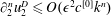 $\unicode[STIX]{x2202}_{2}^{n}u_{2}^{D}\leqslant O(\unicode[STIX]{x1D716}^{2}c^{[0]}k^{n})$
for
$\unicode[STIX]{x2202}_{2}^{n}u_{2}^{D}\leqslant O(\unicode[STIX]{x1D716}^{2}c^{[0]}k^{n})$
for
 $n=0,1,2,3,4$
. Any other derivatives of
$n=0,1,2,3,4$
. Any other derivatives of
 $u_{h}^{D}$
are of third or higher order.
$u_{h}^{D}$
are of third or higher order.
A.2 Derivation of (3.1)
Owing to the horizontal displacement
 $\unicode[STIX]{x1D709}_{h}$
induced by the wave orbital motions, different water parcels within the constant-
$\unicode[STIX]{x1D709}_{h}$
induced by the wave orbital motions, different water parcels within the constant-
 $\unicode[STIX]{x1D701}$
layer at
$\unicode[STIX]{x1D701}$
layer at
 $\unicode[STIX]{x1D701}$
pass back and forth through a given coordinate
$\unicode[STIX]{x1D701}$
pass back and forth through a given coordinate
 $(x,y,\unicode[STIX]{x1D701})$
as
$(x,y,\unicode[STIX]{x1D701})$
as
 $\unicode[STIX]{x1D6E9}$
changes. Thus, if these parcels carry different current velocities, then
$\unicode[STIX]{x1D6E9}$
changes. Thus, if these parcels carry different current velocities, then
 $u_{i}^{c}(x,y,\unicode[STIX]{x1D701},t,\unicode[STIX]{x1D6E9})$
may fluctuate as
$u_{i}^{c}(x,y,\unicode[STIX]{x1D701},t,\unicode[STIX]{x1D6E9})$
may fluctuate as
 $\unicode[STIX]{x1D6E9}$
changes. This fluctuation is equal to
$\unicode[STIX]{x1D6E9}$
changes. This fluctuation is equal to
 $\unicode[STIX]{x1D709}_{1}\unicode[STIX]{x2202}_{1}^{\unicode[STIX]{x1D701}}u_{i}^{c}+\unicode[STIX]{x1D709}_{2}\unicode[STIX]{x2202}_{2}^{\unicode[STIX]{x1D701}}u_{i}^{c}$
, correct to its leading order. Now, the scales of
$\unicode[STIX]{x1D709}_{1}\unicode[STIX]{x2202}_{1}^{\unicode[STIX]{x1D701}}u_{i}^{c}+\unicode[STIX]{x1D709}_{2}\unicode[STIX]{x2202}_{2}^{\unicode[STIX]{x1D701}}u_{i}^{c}$
, correct to its leading order. Now, the scales of
 $a$
and
$a$
and
 $\hat{k}_{2}$
imply that
$\hat{k}_{2}$
imply that
 $\unicode[STIX]{x1D709}_{1}\leqslant O(\unicode[STIX]{x1D716}k^{-1})$
and
$\unicode[STIX]{x1D709}_{1}\leqslant O(\unicode[STIX]{x1D716}k^{-1})$
and
 $\unicode[STIX]{x1D709}_{2}\leqslant O(\unicode[STIX]{x1D716}^{2}k^{-1})$
in accordance with the standard linear wave theory (or see (5.7)). Therefore, this fluctuation in
$\unicode[STIX]{x1D709}_{2}\leqslant O(\unicode[STIX]{x1D716}^{2}k^{-1})$
in accordance with the standard linear wave theory (or see (5.7)). Therefore, this fluctuation in
 $u_{i}^{c}$
is of fourth or higher order. In other words,
$u_{i}^{c}$
is of fourth or higher order. In other words,
 $u_{i}^{c}$
is independent of
$u_{i}^{c}$
is independent of
 $\unicode[STIX]{x1D6E9}$
at least to third order, that is,
$\unicode[STIX]{x1D6E9}$
at least to third order, that is,
 $u_{i}^{c}(x,y,\unicode[STIX]{x1D701},t,\unicode[STIX]{x1D6E9})=u_{i}^{c}(x,y,\unicode[STIX]{x1D701},t)+O(\unicode[STIX]{x1D716}^{4}c^{[0]})$
. Applying (2.5) to this yields (3.1).
$u_{i}^{c}(x,y,\unicode[STIX]{x1D701},t,\unicode[STIX]{x1D6E9})=u_{i}^{c}(x,y,\unicode[STIX]{x1D701},t)+O(\unicode[STIX]{x1D716}^{4}c^{[0]})$
. Applying (2.5) to this yields (3.1).
A.3
$K_{\mathbb{A}(n)}$
and
$K_{\mathbb{B}(n)}$


The scaling conditions (table 4) of
 $\unicode[STIX]{x2202}_{t}^{\unicode[STIX]{x1D701}}u_{(n)}^{c}$
and
$\unicode[STIX]{x2202}_{t}^{\unicode[STIX]{x1D701}}u_{(n)}^{c}$
and
 $\unicode[STIX]{x2202}_{t}^{\unicode[STIX]{x1D701}}w_{(n)}^{c}$
require that
$\unicode[STIX]{x2202}_{t}^{\unicode[STIX]{x1D701}}w_{(n)}^{c}$
require that
 $\unicode[STIX]{x2202}_{t}\sqrt{K_{\mathbb{A}(n)}^{2}-k^{2}}$
and
$\unicode[STIX]{x2202}_{t}\sqrt{K_{\mathbb{A}(n)}^{2}-k^{2}}$
and
 $\unicode[STIX]{x2202}_{t}\sqrt{K_{\mathbb{B}(n)}^{2}-k^{2}}$
be of second or higher order. Likewise,
$\unicode[STIX]{x2202}_{t}\sqrt{K_{\mathbb{B}(n)}^{2}-k^{2}}$
be of second or higher order. Likewise,
 $\unicode[STIX]{x2202}_{h}K_{\mathbb{A}(n)}$
and
$\unicode[STIX]{x2202}_{h}K_{\mathbb{A}(n)}$
and
 $\unicode[STIX]{x2202}_{h}K_{\mathbb{B}(n)}$
as well as any spatial derivatives of
$\unicode[STIX]{x2202}_{h}K_{\mathbb{B}(n)}$
as well as any spatial derivatives of
 $\sqrt{K_{\mathbb{A}(n)}^{2}-k^{2}}$
or
$\sqrt{K_{\mathbb{A}(n)}^{2}-k^{2}}$
or
 $\sqrt{K_{\mathbb{B}(n)}^{2}-k^{2}}$
must be of first or higher order. The upper bounds of
$\sqrt{K_{\mathbb{B}(n)}^{2}-k^{2}}$
must be of first or higher order. The upper bounds of
 $K_{\mathbb{A}(n)}$
and
$K_{\mathbb{A}(n)}$
and
 $K_{\mathbb{B}(n)}$
are due to the scaling conditions
$K_{\mathbb{B}(n)}$
are due to the scaling conditions
 $(\unicode[STIX]{x2202}_{2}^{\unicode[STIX]{x1D701}})^{4}u^{c}\leqslant O(\unicode[STIX]{x1D716}^{3}c^{[0]}k^{4})$
and
$(\unicode[STIX]{x2202}_{2}^{\unicode[STIX]{x1D701}})^{4}u^{c}\leqslant O(\unicode[STIX]{x1D716}^{3}c^{[0]}k^{4})$
and
 $(\unicode[STIX]{x2202}_{2}^{\unicode[STIX]{x1D701}})^{4}w^{c}\leqslant O(\unicode[STIX]{x1D716}^{3}c^{[0]}k^{4})$
.
$(\unicode[STIX]{x2202}_{2}^{\unicode[STIX]{x1D701}})^{4}w^{c}\leqslant O(\unicode[STIX]{x1D716}^{3}c^{[0]}k^{4})$
.
A.4
$C_{(2)}$
,
$C_{(n,3)}$
,
$C_{(n,4)}$
and
$K_{(n)}$


The third-order first-harmonic homogeneous solution
 $P_{\mathbb{H}}^{\{1\}}$
is the solution of
$P_{\mathbb{H}}^{\{1\}}$
is the solution of
 $(\unicode[STIX]{x2202}_{2}^{\unicode[STIX]{x1D701}}\unicode[STIX]{x2202}_{2}^{\unicode[STIX]{x1D701}}+\unicode[STIX]{x2202}_{3}^{\unicode[STIX]{x1D701}}\unicode[STIX]{x2202}_{3}^{\unicode[STIX]{x1D701}}-k^{2})P_{\mathbb{H}}^{\{1\}}=O(\unicode[STIX]{x1D716}^{4}{c^{[0]}}^{2}k^{2})$
. Using a standard method (Kusse & Westwig Reference Kusse and Westwig1998, pp. 424–429) for solving Laplace’s equation, the general homogeneous solution can be obtained as
$(\unicode[STIX]{x2202}_{2}^{\unicode[STIX]{x1D701}}\unicode[STIX]{x2202}_{2}^{\unicode[STIX]{x1D701}}+\unicode[STIX]{x2202}_{3}^{\unicode[STIX]{x1D701}}\unicode[STIX]{x2202}_{3}^{\unicode[STIX]{x1D701}}-k^{2})P_{\mathbb{H}}^{\{1\}}=O(\unicode[STIX]{x1D716}^{4}{c^{[0]}}^{2}k^{2})$
. Using a standard method (Kusse & Westwig Reference Kusse and Westwig1998, pp. 424–429) for solving Laplace’s equation, the general homogeneous solution can be obtained as
 $$\begin{eqnarray}\displaystyle P_{\mathbb{H}}^{\{1\}} & = & \displaystyle (C_{(1)}y+C_{(2)})\text{e}^{k\unicode[STIX]{x1D701}}+\mathop{\sum }_{n\geqslant 1}(C_{(n,1)}\text{e}^{\sqrt{k^{2}-k_{(n)}^{2}}y}+C_{(n,2)}\text{e}^{-\sqrt{k^{2}-k_{(n)}^{2}}y})\text{e}^{k_{(n)}\unicode[STIX]{x1D701}}\nonumber\\ \displaystyle & & \displaystyle +\,\mathop{\sum }_{n\geqslant 1}C_{(n,3)}\cos \left(\sqrt{K_{(n)}^{2}-k^{2}}y+C_{(n,4)}\right)\text{e}^{K_{(n)}\unicode[STIX]{x1D701}},\end{eqnarray}$$
where the parameters
 $C_{(m)}$
and
$C_{(m)}$
and
 $C_{(n,m)}$
for
$C_{(n,m)}$
for
 $m=1,2,3$
are complex;
$m=1,2,3$
are complex;
 $C_{(n,4)}$
,
$C_{(n,4)}$
,
 $k_{(n)}$
and
$k_{(n)}$
and
 $K_{(n)}$
are real; and
$K_{(n)}$
are real; and
 $0<k_{(n)}<k<K_{(n)}$
. These parameters are constants or functions of
$0<k_{(n)}<k<K_{(n)}$
. These parameters are constants or functions of
 $(x,y,t)$
, but their horizontal gradients must be negligible for the third-order balance: that is,
$(x,y,t)$
, but their horizontal gradients must be negligible for the third-order balance: that is,
 $\unicode[STIX]{x2202}_{h}C_{(1)}$
,
$\unicode[STIX]{x2202}_{h}C_{(1)}$
,
 $\unicode[STIX]{x2202}_{1}C_{(2)}$
and
$\unicode[STIX]{x2202}_{1}C_{(2)}$
and
 $\unicode[STIX]{x2202}_{h}C_{(n,m)}$
(for
$\unicode[STIX]{x2202}_{h}C_{(n,m)}$
(for
 $m=1,2,3$
), and
$m=1,2,3$
), and
 $\unicode[STIX]{x2202}_{2}\unicode[STIX]{x2202}_{2}C_{(2)}$
must be of fourth or higher order; and
$\unicode[STIX]{x2202}_{2}\unicode[STIX]{x2202}_{2}C_{(2)}$
must be of fourth or higher order; and
 $\unicode[STIX]{x2202}_{h}C_{(n,4)}$
,
$\unicode[STIX]{x2202}_{h}C_{(n,4)}$
,
 $\unicode[STIX]{x2202}_{h}k_{(n)}$
and
$\unicode[STIX]{x2202}_{h}k_{(n)}$
and
 $\unicode[STIX]{x2202}_{h}K_{(n)}$
, as well as any spatial derivatives of
$\unicode[STIX]{x2202}_{h}K_{(n)}$
, as well as any spatial derivatives of
 $\sqrt{k^{2}-k_{(n)}^{2}}$
and
$\sqrt{k^{2}-k_{(n)}^{2}}$
and
 $\sqrt{K_{(n)}^{2}-k^{2}}$
, must be of first or higher order. These parameters are to be determined by some constraints such as the horizontal boundary condition. For simplicity, S19 specifies some degree of constraints with regard to the horizontal boundary condition, or equivalently
$\sqrt{K_{(n)}^{2}-k^{2}}$
, must be of first or higher order. These parameters are to be determined by some constraints such as the horizontal boundary condition. For simplicity, S19 specifies some degree of constraints with regard to the horizontal boundary condition, or equivalently
 $P_{\mathbb{H}}^{\{1\}}$
. Namely, S19 considers only those
$P_{\mathbb{H}}^{\{1\}}$
. Namely, S19 considers only those
 $P_{\mathbb{H}}^{\{1\}}$
whose structures are similar to that of the current, and whose time scales satisfy
$P_{\mathbb{H}}^{\{1\}}$
whose structures are similar to that of the current, and whose time scales satisfy
 $\unicode[STIX]{x2202}_{t}^{\unicode[STIX]{x1D701}}\unicode[STIX]{x2202}_{t}^{\unicode[STIX]{x1D701}}P_{\mathbb{H}}^{\{1\}}\leqslant O(\unicode[STIX]{x1D716}^{4}{c^{[0]}}^{4}k^{2})$
. In other words,
$\unicode[STIX]{x2202}_{t}^{\unicode[STIX]{x1D701}}\unicode[STIX]{x2202}_{t}^{\unicode[STIX]{x1D701}}P_{\mathbb{H}}^{\{1\}}\leqslant O(\unicode[STIX]{x1D716}^{4}{c^{[0]}}^{4}k^{2})$
. In other words,
 $C_{(1)}=0$
,
$C_{(1)}=0$
,
 $C_{(n,1)}=0$
,
$C_{(n,1)}=0$
,
 $C_{(n,2)}=0$
,
$C_{(n,2)}=0$
,
 $K_{(n)}\leqslant 1.15k$
,
$K_{(n)}\leqslant 1.15k$
,
 $\unicode[STIX]{x2202}_{t}\unicode[STIX]{x2202}_{t}C_{(2)}\leqslant O(\unicode[STIX]{x1D716}^{4}{c^{[0]}}^{4}k^{2})$
,
$\unicode[STIX]{x2202}_{t}\unicode[STIX]{x2202}_{t}C_{(2)}\leqslant O(\unicode[STIX]{x1D716}^{4}{c^{[0]}}^{4}k^{2})$
,
 $\unicode[STIX]{x2202}_{t}\unicode[STIX]{x2202}_{t}C_{(n,3)}\leqslant O(\unicode[STIX]{x1D716}^{4}{c^{[0]}}^{4}k^{2})$
,
$\unicode[STIX]{x2202}_{t}\unicode[STIX]{x2202}_{t}C_{(n,3)}\leqslant O(\unicode[STIX]{x1D716}^{4}{c^{[0]}}^{4}k^{2})$
,
 $\unicode[STIX]{x2202}_{t}C_{(n,4)}\leqslant O(\unicode[STIX]{x1D716}c^{[0]}k)$
,
$\unicode[STIX]{x2202}_{t}C_{(n,4)}\leqslant O(\unicode[STIX]{x1D716}c^{[0]}k)$
,
 $\unicode[STIX]{x2202}_{t}K_{(n)}\leqslant O(\unicode[STIX]{x1D716}c^{[0]}k^{2})$
,
$\unicode[STIX]{x2202}_{t}K_{(n)}\leqslant O(\unicode[STIX]{x1D716}c^{[0]}k^{2})$
,
 $\unicode[STIX]{x2202}_{t}\sqrt{K_{(n)}^{2}-k^{2}}\leqslant O(\unicode[STIX]{x1D716}c^{[0]}k^{2})$
and
$\unicode[STIX]{x2202}_{t}\sqrt{K_{(n)}^{2}-k^{2}}\leqslant O(\unicode[STIX]{x1D716}c^{[0]}k^{2})$
and
 $\unicode[STIX]{x2202}_{t}\unicode[STIX]{x2202}_{t}\sqrt{K_{(n)}^{2}-k^{2}}\leqslant O(\unicode[STIX]{x1D716}{c^{[0]}}^{2}k^{3})$
. This results in (5.23a
).
$\unicode[STIX]{x2202}_{t}\unicode[STIX]{x2202}_{t}\sqrt{K_{(n)}^{2}-k^{2}}\leqslant O(\unicode[STIX]{x1D716}{c^{[0]}}^{2}k^{3})$
. This results in (5.23a
).
Appendix B. The third-order governing equations
Substitute (5.7), (5.9) and (5.10) into (5.1)–(5.5) to obtain the third-order governing equations for each harmonic. In this step, we can use the fact that
 $\unicode[STIX]{x2202}_{1}^{\unicode[STIX]{x1D701}}u_{i}^{\{n\}}$
,
$\unicode[STIX]{x2202}_{1}^{\unicode[STIX]{x1D701}}u_{i}^{\{n\}}$
,
 $\unicode[STIX]{x2202}_{1}^{\unicode[STIX]{x1D701}}P^{\{n\}}$
and
$\unicode[STIX]{x2202}_{1}^{\unicode[STIX]{x1D701}}P^{\{n\}}$
and
 $\unicode[STIX]{x2202}_{1}^{\unicode[STIX]{x1D701}}z^{\{n\}}$
are of fourth or higher order. (This fact is verified for the derived solutions and the scaling conditions listed in § 3.) Unlike the
$\unicode[STIX]{x2202}_{1}^{\unicode[STIX]{x1D701}}z^{\{n\}}$
are of fourth or higher order. (This fact is verified for the derived solutions and the scaling conditions listed in § 3.) Unlike the
 $x$
-derivatives, the
$x$
-derivatives, the
 $y$
-,
$y$
-,
 $t$
- and
$t$
- and
 $\unicode[STIX]{x1D701}$
-derivatives of
$\unicode[STIX]{x1D701}$
-derivatives of
 $u_{i}^{\{n\}}$
,
$u_{i}^{\{n\}}$
,
 $P^{\{n\}}$
and
$P^{\{n\}}$
and
 $z^{\{n\}}$
cannot be neglected. The momentum equations (5.1) yield
$z^{\{n\}}$
cannot be neglected. The momentum equations (5.1) yield
 $$\begin{eqnarray}\displaystyle u^{\{1\}} & = & \displaystyle \frac{\hat{k}_{1}}{c^{[0]}}P^{\{1\}}-\text{i}\frac{1}{c^{[0]}k}\unicode[STIX]{x2202}_{t}^{\unicode[STIX]{x1D701}}u^{\{1\}}-\text{i}\frac{\hat{k}_{1}}{c^{[0]}k}\unicode[STIX]{x2202}_{t}^{\unicode[STIX]{x1D701}}(c^{[0]}ak\text{e}^{k\unicode[STIX]{x1D701}})-\text{i}c^{[0]}\unicode[STIX]{x2202}_{1}^{\unicode[STIX]{x1D701}}(a\text{e}^{k\unicode[STIX]{x1D701}})-\text{i}a\text{e}^{k\unicode[STIX]{x1D701}}\unicode[STIX]{x2202}_{t}\hat{k}_{1}\nonumber\\ \displaystyle & & \displaystyle +\,\hat{k}_{1}ak\text{e}^{k\unicode[STIX]{x1D701}}\left(\hat{k}_{1}u_{1}^{c}-\hat{k}_{1}u_{1}^{D}+\hat{k}_{1}\mathfrak{U}_{1}-c^{[2]}+\frac{1}{2}c^{[0]}a^{2}k^{2}\text{e}^{2k\unicode[STIX]{x1D701}}-\text{i}w^{c}\right)+O(\unicode[STIX]{x1D716}^{4}c^{[0]}),\qquad\end{eqnarray}$$
 $$\begin{eqnarray}v^{\{1\}}=-\text{i}\frac{1}{c^{[0]}k}\unicode[STIX]{x2202}_{2}^{\unicode[STIX]{x1D701}}P^{\{1\}}-\text{i}\frac{1}{c^{[0]}k}\unicode[STIX]{x2202}_{t}^{\unicode[STIX]{x1D701}}v^{\{1\}}-\text{i}c^{[0]}\unicode[STIX]{x2202}_{2}^{\unicode[STIX]{x1D701}}(a\text{e}^{k\unicode[STIX]{x1D701}})-\text{i}a\text{e}^{k\unicode[STIX]{x1D701}}\unicode[STIX]{x2202}_{t}\hat{k}_{2}+O(\unicode[STIX]{x1D716}^{4}c^{[0]}),\end{eqnarray}$$
 $$\begin{eqnarray}\displaystyle w^{\{1\}} & = & \displaystyle -\text{i}\frac{1}{c^{[0]}k}\unicode[STIX]{x2202}_{3}^{\unicode[STIX]{x1D701}}P^{\{1\}}-\text{i}\frac{1}{c^{[0]}k}\unicode[STIX]{x2202}_{t}^{\unicode[STIX]{x1D701}}w^{\{1\}}-\frac{1}{c^{[0]}k}\unicode[STIX]{x2202}_{t}^{\unicode[STIX]{x1D701}}(c^{[0]}ak\text{e}^{k\unicode[STIX]{x1D701}})\nonumber\\ \displaystyle & & \displaystyle -\,\text{i}ak\text{e}^{k\unicode[STIX]{x1D701}}\left(\hat{k}_{1}u_{1}^{c}-\hat{k}_{1}u_{1}^{D}+\hat{k}_{1}\mathfrak{U}_{1}-c^{[2]}+\frac{1}{2}c^{[0]}a^{2}k^{2}\text{e}^{2k\unicode[STIX]{x1D701}}-\text{i}w^{c}\right)+O(\unicode[STIX]{x1D716}^{4}c^{[0]}),\qquad\end{eqnarray}$$
 $$\begin{eqnarray}\displaystyle & \displaystyle u^{\{2\}}=\frac{\hat{k}_{1}}{c^{[0]}}P^{\{2\}}-\frac{\text{i}}{2c^{[0]}k}\unicode[STIX]{x2202}_{t}^{\unicode[STIX]{x1D701}}u^{\{2\}}+O(\unicode[STIX]{x1D716}^{4}c^{[0]}), & \displaystyle\end{eqnarray}$$
 $$\begin{eqnarray}\displaystyle & \displaystyle v^{\{2\}}=-\frac{\text{i}}{2c^{[0]}k}\unicode[STIX]{x2202}_{2}^{\unicode[STIX]{x1D701}}P^{\{2\}}-\frac{\text{i}}{2c^{[0]}k}\unicode[STIX]{x2202}_{t}^{\unicode[STIX]{x1D701}}v^{\{2\}}+O(\unicode[STIX]{x1D716}^{4}c^{[0]}), & \displaystyle\end{eqnarray}$$
 $$\begin{eqnarray}\displaystyle & \displaystyle w^{\{2\}}=-\frac{\text{i}}{2c^{[0]}k}\unicode[STIX]{x2202}_{3}^{\unicode[STIX]{x1D701}}P^{\{2\}}-\frac{\text{i}}{2c^{[0]}k}\unicode[STIX]{x2202}_{t}^{\unicode[STIX]{x1D701}}w^{\{2\}}+O(\unicode[STIX]{x1D716}^{4}c^{[0]}), & \displaystyle\end{eqnarray}$$
 $$\begin{eqnarray}\displaystyle & \displaystyle u^{\{3\}}=\frac{\hat{k}_{1}}{c^{[0]}}P^{\{3\}}-\frac{\text{i}}{3c^{[0]}k}\unicode[STIX]{x2202}_{t}^{\unicode[STIX]{x1D701}}u^{\{3\}}+O(\unicode[STIX]{x1D716}^{4}c^{[0]}), & \displaystyle\end{eqnarray}$$
 $$\begin{eqnarray}\displaystyle & \displaystyle v^{\{3\}}=-\frac{\text{i}}{3c^{[0]}k}\unicode[STIX]{x2202}_{2}^{\unicode[STIX]{x1D701}}P^{\{3\}}-\frac{\text{i}}{3c^{[0]}k}\unicode[STIX]{x2202}_{t}^{\unicode[STIX]{x1D701}}v^{\{3\}}+O(\unicode[STIX]{x1D716}^{4}c^{[0]}), & \displaystyle\end{eqnarray}$$
 $$\begin{eqnarray}\displaystyle & \displaystyle w^{\{3\}}=-\frac{\text{i}}{3c^{[0]}k}\unicode[STIX]{x2202}_{3}^{\unicode[STIX]{x1D701}}P^{\{3\}}-\frac{\text{i}}{3c^{[0]}k}\unicode[STIX]{x2202}_{t}^{\unicode[STIX]{x1D701}}w^{\{3\}}+O(\unicode[STIX]{x1D716}^{4}c^{[0]}). & \displaystyle\end{eqnarray}$$
 $$\begin{eqnarray}\displaystyle & & \displaystyle \text{i}\hat{k}_{1}ku^{\{1\}}+\unicode[STIX]{x2202}_{2}^{\unicode[STIX]{x1D701}}v^{\{1\}}+\unicode[STIX]{x2202}_{3}^{\unicode[STIX]{x1D701}}w^{\{1\}}-ak\text{e}^{k\unicode[STIX]{x1D701}}[\text{i}\hat{k}_{1}\unicode[STIX]{x2202}_{3}^{\unicode[STIX]{x1D701}}(u_{1}^{c}+\mathfrak{U}_{1})+\unicode[STIX]{x2202}_{3}^{\unicode[STIX]{x1D701}}w^{c}]\nonumber\\ \displaystyle & & \displaystyle \quad +\,c^{[0]}ak\text{e}^{k\unicode[STIX]{x1D701}}\unicode[STIX]{x2202}_{H}\hat{k}_{H}+\hat{k}_{1}\unicode[STIX]{x2202}_{1}^{\unicode[STIX]{x1D701}}(c^{[0]}ak\text{e}^{k\unicode[STIX]{x1D701}})=O(\unicode[STIX]{x1D716}^{4}c^{[0]}k),\end{eqnarray}$$
 $$\begin{eqnarray}\displaystyle & \displaystyle \text{i}2\hat{k}_{1}ku^{\{2\}}+\unicode[STIX]{x2202}_{2}^{\unicode[STIX]{x1D701}}v^{\{2\}}+\unicode[STIX]{x2202}_{3}^{\unicode[STIX]{x1D701}}w^{\{2\}}=O(\unicode[STIX]{x1D716}^{4}c^{[0]}k), & \displaystyle\end{eqnarray}$$
 $$\begin{eqnarray}\displaystyle & \displaystyle \text{i}3\hat{k}_{1}ku^{\{3\}}+\unicode[STIX]{x2202}_{2}^{\unicode[STIX]{x1D701}}v^{\{3\}}+\unicode[STIX]{x2202}_{3}^{\unicode[STIX]{x1D701}}w^{\{3\}}=O(\unicode[STIX]{x1D716}^{4}c^{[0]}k). & \displaystyle\end{eqnarray}$$
 $$\begin{eqnarray}\displaystyle & \displaystyle \text{i}\hat{k}_{1}k\unicode[STIX]{x2202}_{t}^{\unicode[STIX]{x1D701}}u^{\{1\}}+\unicode[STIX]{x2202}_{2}^{\unicode[STIX]{x1D701}}\unicode[STIX]{x2202}_{t}^{\unicode[STIX]{x1D701}}v^{\{1\}}+\unicode[STIX]{x2202}_{3}^{\unicode[STIX]{x1D701}}\unicode[STIX]{x2202}_{t}^{\unicode[STIX]{x1D701}}w^{\{1\}}+c^{[0]}ak\text{e}^{k\unicode[STIX]{x1D701}}\unicode[STIX]{x2202}_{2}\unicode[STIX]{x2202}_{t}\hat{k}_{2}=O(\unicode[STIX]{x1D716}^{4}{c^{[0]}}^{2}k^{2}), & \displaystyle\end{eqnarray}$$
 $$\begin{eqnarray}\displaystyle & \displaystyle \text{i}2\hat{k}_{1}k\unicode[STIX]{x2202}_{t}^{\unicode[STIX]{x1D701}}u^{\{2\}}+\unicode[STIX]{x2202}_{2}^{\unicode[STIX]{x1D701}}\unicode[STIX]{x2202}_{t}^{\unicode[STIX]{x1D701}}v^{\{2\}}+\unicode[STIX]{x2202}_{3}^{\unicode[STIX]{x1D701}}\unicode[STIX]{x2202}_{t}^{\unicode[STIX]{x1D701}}w^{\{2\}}=O(\unicode[STIX]{x1D716}^{4}{c^{[0]}}^{2}k^{2}), & \displaystyle\end{eqnarray}$$
 $$\begin{eqnarray}\displaystyle & \displaystyle \text{i}3\hat{k}_{1}k\unicode[STIX]{x2202}_{t}^{\unicode[STIX]{x1D701}}u^{\{3\}}+\unicode[STIX]{x2202}_{2}^{\unicode[STIX]{x1D701}}\unicode[STIX]{x2202}_{t}^{\unicode[STIX]{x1D701}}v^{\{3\}}+\unicode[STIX]{x2202}_{3}^{\unicode[STIX]{x1D701}}\unicode[STIX]{x2202}_{t}^{\unicode[STIX]{x1D701}}w^{\{3\}}=O(\unicode[STIX]{x1D716}^{4}{c^{[0]}}^{2}k^{2}). & \displaystyle\end{eqnarray}$$
 $$\begin{eqnarray}u_{i}^{\{n\}}=O(\unicode[STIX]{x1D716}^{4}c^{[0]})\quad \text{at }\unicode[STIX]{x1D701}=-\infty\end{eqnarray}$$
for
 $n=1,2,3$
. Then, (B 1a
), (B 1d
), (B 1g
) and (B 4) yield
$n=1,2,3$
. Then, (B 1a
), (B 1d
), (B 1g
) and (B 4) yield
 $$\begin{eqnarray}P^{\{n\}}=O(\unicode[STIX]{x1D716}^{4}{c^{[0]}}^{2})\quad \text{at }\unicode[STIX]{x1D701}=-\infty .\end{eqnarray}$$
The upper boundary condition (5.5) yields
 $$\begin{eqnarray}\displaystyle & & \displaystyle -\text{i}\frac{P^{\{1\}}}{c^{[0]}}+\frac{1}{g}\unicode[STIX]{x2202}_{t}^{\unicode[STIX]{x1D701}}P^{\{1\}}-w^{\{1\}}+\unicode[STIX]{x2202}_{t}a\nonumber\\ \displaystyle & & \displaystyle \quad +\,\text{i}ak\left(\hat{k}_{1}u_{1}^{c}-\hat{k}_{1}u_{1}^{D}+\hat{k}_{1}\mathfrak{U}_{1}-c^{[2]}+\frac{1}{4}c^{[0]}a^{2}k^{2}\right)=O(\unicode[STIX]{x1D716}^{4}c^{[0]})\quad \text{at }\unicode[STIX]{x1D701}=0,\qquad\end{eqnarray}$$
 $$\begin{eqnarray}\displaystyle & \displaystyle -\text{i}2\frac{P^{\{2\}}}{c^{[0]}}+\frac{1}{g}\unicode[STIX]{x2202}_{t}^{\unicode[STIX]{x1D701}}P^{\{2\}}-w^{\{2\}}=O(\unicode[STIX]{x1D716}^{4}c^{[0]})\quad \text{at }\unicode[STIX]{x1D701}=0, & \displaystyle\end{eqnarray}$$
 $$\begin{eqnarray}\displaystyle & \displaystyle -\text{i}3\frac{P^{\{3\}}}{c^{[0]}}+\frac{1}{g}\unicode[STIX]{x2202}_{t}^{\unicode[STIX]{x1D701}}P^{\{3\}}-w^{\{3\}}+\text{i}\frac{3}{4}c^{[0]}a^{3}k^{3}=O(\unicode[STIX]{x1D716}^{4}c^{[0]})\quad \text{at }\unicode[STIX]{x1D701}=0. & \displaystyle\end{eqnarray}$$
 $\unicode[STIX]{x1D701}$
-surfaces (5.3) yields
$\unicode[STIX]{x1D701}$
-surfaces (5.3) yields  $$\begin{eqnarray}\displaystyle kz^{\{1\}} & = & \displaystyle -\text{i}\frac{1}{c^{[0]}}\unicode[STIX]{x2202}_{t}^{\unicode[STIX]{x1D701}}z^{\{1\}}+\text{i}\frac{w^{\{1\}}}{c^{[0]}}-\text{i}\frac{\unicode[STIX]{x2202}_{t}^{\unicode[STIX]{x1D701}}(a\text{e}^{k\unicode[STIX]{x1D701}})}{c^{[0]}}\nonumber\\ \displaystyle & & \displaystyle \quad +\,\frac{1}{c^{[0]}}ak\text{e}^{k\unicode[STIX]{x1D701}}\left(\hat{k}_{1}u_{1}^{c}-\hat{k}_{1}u_{1}^{D}+\hat{k}_{1}\mathfrak{U}_{1}-c^{[2]}+\frac{1}{4}c^{[0]}a^{2}k^{2}\text{e}^{2k\unicode[STIX]{x1D701}}\right)+O(\unicode[STIX]{x1D716}^{4}),\qquad\end{eqnarray}$$
 $$\begin{eqnarray}\displaystyle & \displaystyle kz^{\{2\}}=-\text{i}\frac{1}{2c^{[0]}}\unicode[STIX]{x2202}_{t}^{\unicode[STIX]{x1D701}}z^{\{2\}}+\text{i}\frac{w^{\{2\}}}{2c^{[0]}}+O(\unicode[STIX]{x1D716}^{4}), & \displaystyle\end{eqnarray}$$
 $$\begin{eqnarray}\displaystyle & \displaystyle kz^{\{3\}}=-\text{i}\frac{1}{3c^{[0]}}\unicode[STIX]{x2202}_{t}^{\unicode[STIX]{x1D701}}z^{\{3\}}+\text{i}\frac{w^{\{3\}}}{3c^{[0]}}+\frac{1}{4}a^{3}k^{3}\text{e}^{3k\unicode[STIX]{x1D701}}+O(\unicode[STIX]{x1D716}^{4}). & \displaystyle\end{eqnarray}$$
Appendix C. Useful identities
Because
 $\hat{k}_{h}\hat{k}_{h}=1$
, we have
$\hat{k}_{h}\hat{k}_{h}=1$
, we have
 $\hat{k}_{h}\unicode[STIX]{x2202}_{\ell }\hat{k}_{h}=(1/2)\unicode[STIX]{x2202}_{\ell }(\hat{k}_{h}\hat{k}_{h})=0$
. This and the scaling conditions for the zeroth and first derivatives listed in § 3 yield
$\hat{k}_{h}\unicode[STIX]{x2202}_{\ell }\hat{k}_{h}=(1/2)\unicode[STIX]{x2202}_{\ell }(\hat{k}_{h}\hat{k}_{h})=0$
. This and the scaling conditions for the zeroth and first derivatives listed in § 3 yield
 $$\begin{eqnarray}\hat{k}_{1}\unicode[STIX]{x2202}_{\ell }\hat{k}_{1}=-\hat{k}_{2}\unicode[STIX]{x2202}_{\ell }\hat{k}_{2}\leqslant \left\{\begin{array}{@{}ll@{}}O(\unicode[STIX]{x1D716}^{3}k), & \text{for }\ell =1,2,3,\\ O(\unicode[STIX]{x1D716}^{3}c^{[0]}k), & \text{for }\ell =t.\end{array}\right.\end{eqnarray}$$
Because
 $\unicode[STIX]{x2202}_{1}\unicode[STIX]{x2202}_{2}\unicode[STIX]{x1D712}=\unicode[STIX]{x2202}_{2}\unicode[STIX]{x2202}_{1}\unicode[STIX]{x1D712}$
, equation (2.3) gives
$\unicode[STIX]{x2202}_{1}\unicode[STIX]{x2202}_{2}\unicode[STIX]{x1D712}=\unicode[STIX]{x2202}_{2}\unicode[STIX]{x2202}_{1}\unicode[STIX]{x1D712}$
, equation (2.3) gives
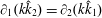 $\unicode[STIX]{x2202}_{1}(k\hat{k}_{2})=\unicode[STIX]{x2202}_{2}(k\hat{k}_{1})$
. This and the scaling for the zeroth and first derivatives (§ 3) yield
$\unicode[STIX]{x2202}_{1}(k\hat{k}_{2})=\unicode[STIX]{x2202}_{2}(k\hat{k}_{1})$
. This and the scaling for the zeroth and first derivatives (§ 3) yield
 $$\begin{eqnarray}\unicode[STIX]{x2202}_{2}k=k\hat{k}_{1}\unicode[STIX]{x2202}_{1}\hat{k}_{2}+O(\unicode[STIX]{x1D716}^{3}k^{2}),\quad -\unicode[STIX]{x2202}_{h}k+\hat{k}_{h}\hat{k}_{1}\unicode[STIX]{x2202}_{1}k+k\hat{k}_{1}\unicode[STIX]{x2202}_{1}\hat{k}_{h}=O(\unicode[STIX]{x1D716}^{3}k^{2}).\end{eqnarray}$$
Equations (5.11), (5.12) and (5.13) and the scaling for the zeroth and first derivatives (§ 3) yield
 $$\begin{eqnarray}\displaystyle & \displaystyle \unicode[STIX]{x2202}_{t}k=-\frac{c^{[0]}}{2}\hat{k}_{1}\unicode[STIX]{x2202}_{1}k+O(\unicode[STIX]{x1D716}^{3}c^{[0]}k^{2}), & \displaystyle\end{eqnarray}$$
 $$\begin{eqnarray}\displaystyle & \displaystyle \unicode[STIX]{x2202}_{t}\hat{k}_{1}=-\frac{\hat{k}_{1}}{k}\unicode[STIX]{x2202}_{t}k-\frac{c^{[0]}}{2k}\unicode[STIX]{x2202}_{1}k+O(\unicode[STIX]{x1D716}^{3}c^{[0]}k), & \displaystyle\end{eqnarray}$$
 $$\begin{eqnarray}\displaystyle & \displaystyle \unicode[STIX]{x2202}_{t}\hat{k}_{2}=-\frac{c^{[0]}}{2k}\unicode[STIX]{x2202}_{2}k-\unicode[STIX]{x2202}_{2}c^{[2]}-\hat{k}_{1}\unicode[STIX]{x2202}_{2}u_{1}^{D}+O(\unicode[STIX]{x1D716}^{3}c^{[0]}k). & \displaystyle\end{eqnarray}$$
Therefore,
 $\unicode[STIX]{x2202}_{t}\hat{k}_{1}=O(\unicode[STIX]{x1D716}^{3}c^{[0]}k)$
and
$\unicode[STIX]{x2202}_{t}\hat{k}_{1}=O(\unicode[STIX]{x1D716}^{3}c^{[0]}k)$
and
 $\unicode[STIX]{x2202}_{t}^{\unicode[STIX]{x1D701}}\text{e}^{nk\unicode[STIX]{x1D701}}=-(1/2)c^{[0]}\hat{k}_{1}\unicode[STIX]{x2202}_{1}^{\unicode[STIX]{x1D701}}\text{e}^{nk\unicode[STIX]{x1D701}}+O(n\unicode[STIX]{x1D716}^{3}c^{[0]}k)$
for any real number
$\unicode[STIX]{x2202}_{t}^{\unicode[STIX]{x1D701}}\text{e}^{nk\unicode[STIX]{x1D701}}=-(1/2)c^{[0]}\hat{k}_{1}\unicode[STIX]{x2202}_{1}^{\unicode[STIX]{x1D701}}\text{e}^{nk\unicode[STIX]{x1D701}}+O(n\unicode[STIX]{x1D716}^{3}c^{[0]}k)$
for any real number
 $n$
. From (C 1), (C 2), (5.11), (5.14b
) and
$n$
. From (C 1), (C 2), (5.11), (5.14b
) and
 $U_{h}^{S}\equiv c^{[0]}a^{2}k^{2}\text{e}^{2k\unicode[STIX]{x1D701}}\hat{k}_{h}$
, we have
$U_{h}^{S}\equiv c^{[0]}a^{2}k^{2}\text{e}^{2k\unicode[STIX]{x1D701}}\hat{k}_{h}$
, we have
 $$\begin{eqnarray}\displaystyle c_{H}^{g}\unicode[STIX]{x2202}_{H}^{\unicode[STIX]{x1D701}}({\textstyle \frac{1}{2}}U_{1}^{S}) & = & \displaystyle c_{H}^{g}c^{[0]}ak^{2}\text{e}^{2k\unicode[STIX]{x1D701}}\hat{k}_{1}\unicode[STIX]{x2202}_{H}a+{\textstyle \frac{1}{2}}{c^{[0]}}^{2}a^{2}k^{2}\text{e}^{k\unicode[STIX]{x1D701}}\unicode[STIX]{x2202}_{1}^{\unicode[STIX]{x1D701}}\text{e}^{k\unicode[STIX]{x1D701}}\nonumber\\ \displaystyle & & \displaystyle +\,{\textstyle \frac{3}{8}}{c^{[0]}}^{2}a^{2}k\text{e}^{2k\unicode[STIX]{x1D701}}\unicode[STIX]{x2202}_{1}k+O(\unicode[STIX]{x1D716}^{5}{c^{[0]}}^{2}k),\end{eqnarray}$$
 $$\begin{eqnarray}c_{H}^{g}\unicode[STIX]{x2202}_{H}^{\unicode[STIX]{x1D701}}({\textstyle \frac{1}{2}}U_{2}^{S})={\textstyle \frac{1}{4}}{c^{[0]}}^{2}a^{2}k\text{e}^{2k\unicode[STIX]{x1D701}}\unicode[STIX]{x2202}_{2}k+O(\unicode[STIX]{x1D716}^{5}{c^{[0]}}^{2}k)=-U_{H}^{S}\unicode[STIX]{x2202}_{2}^{\unicode[STIX]{x1D701}}c_{H}^{g}+O(\unicode[STIX]{x1D716}^{5}{c^{[0]}}^{2}k).\end{eqnarray}$$
Appendix D. Derivation of the third-order wave solutions
Combining (5.7e
), (5.11), (B 1a
)–(B 1c
), (B 2a
), (B 3a
) and
 $\hat{k}_{h}\unicode[STIX]{x2202}_{\ell }\hat{k}_{h}=0$
yields the governing equation for
$\hat{k}_{h}\unicode[STIX]{x2202}_{\ell }\hat{k}_{h}=0$
yields the governing equation for
 $P^{\{1\}}$
as
$P^{\{1\}}$
as
 $(\unicode[STIX]{x2202}_{2}^{\unicode[STIX]{x1D701}}\unicode[STIX]{x2202}_{2}^{\unicode[STIX]{x1D701}}+\unicode[STIX]{x2202}_{3}^{\unicode[STIX]{x1D701}}\unicode[STIX]{x2202}_{3}^{\unicode[STIX]{x1D701}}-k^{2})P^{\{1\}}+\mathbb{A}+\mathbb{B}+\mathbb{C}+\mathbb{D}+\mathbb{E}+\mathbb{F}=O(\unicode[STIX]{x1D716}^{4}{c^{[0]}}^{2}k^{2})$
, where the six driving functions are defined in table 1. The solution satisfying the lower boundary condition (B 5) is
$(\unicode[STIX]{x2202}_{2}^{\unicode[STIX]{x1D701}}\unicode[STIX]{x2202}_{2}^{\unicode[STIX]{x1D701}}+\unicode[STIX]{x2202}_{3}^{\unicode[STIX]{x1D701}}\unicode[STIX]{x2202}_{3}^{\unicode[STIX]{x1D701}}-k^{2})P^{\{1\}}+\mathbb{A}+\mathbb{B}+\mathbb{C}+\mathbb{D}+\mathbb{E}+\mathbb{F}=O(\unicode[STIX]{x1D716}^{4}{c^{[0]}}^{2}k^{2})$
, where the six driving functions are defined in table 1. The solution satisfying the lower boundary condition (B 5) is
 $$\begin{eqnarray}P^{\{1\}}=P_{\mathbb{ H}}^{\{1\}}+P_{\mathbb{ A}}^{\{1\}}+P_{\mathbb{ B}}^{\{1\}}+P_{\mathbb{ C}}^{\{1\}}+P_{\mathbb{ D}}^{\{1\}}+P_{\mathbb{ E}}^{\{1\}}+P_{\mathbb{ F}}^{\{1\}},\end{eqnarray}$$
where the terms on the right-hand side are given by (5.23a
), (5.26a
), (5.29a
), (5.32a
), (5.36a
), (5.39a
) and (5.42a
). Here,
 $P_{\mathbb{H}}^{\{1\}}$
is the homogeneous solution, and
$P_{\mathbb{H}}^{\{1\}}$
is the homogeneous solution, and
 $P_{\mathbb{A}}^{\{1\}}$
through
$P_{\mathbb{A}}^{\{1\}}$
through
 $P_{\mathbb{F}}^{\{1\}}$
are the particular solutions for the corresponding driving functions: that is,
$P_{\mathbb{F}}^{\{1\}}$
are the particular solutions for the corresponding driving functions: that is,
 $(\unicode[STIX]{x2202}_{2}^{\unicode[STIX]{x1D701}}\unicode[STIX]{x2202}_{2}^{\unicode[STIX]{x1D701}}+\unicode[STIX]{x2202}_{3}^{\unicode[STIX]{x1D701}}\unicode[STIX]{x2202}_{3}^{\unicode[STIX]{x1D701}}-k^{2})P_{\mathbb{A}}^{\{1\}}+\mathbb{A}=O(\unicode[STIX]{x1D716}^{4}{c^{[0]}}^{2}k^{2})$
, and so on. The expression for
$(\unicode[STIX]{x2202}_{2}^{\unicode[STIX]{x1D701}}\unicode[STIX]{x2202}_{2}^{\unicode[STIX]{x1D701}}+\unicode[STIX]{x2202}_{3}^{\unicode[STIX]{x1D701}}\unicode[STIX]{x2202}_{3}^{\unicode[STIX]{x1D701}}-k^{2})P_{\mathbb{A}}^{\{1\}}+\mathbb{A}=O(\unicode[STIX]{x1D716}^{4}{c^{[0]}}^{2}k^{2})$
, and so on. The expression for
 $P_{\mathbb{H}}^{\{1\}}$
is derived in § A.4;
$P_{\mathbb{H}}^{\{1\}}$
is derived in § A.4;
 $P_{\mathbb{A}}^{\{1\}}$
and
$P_{\mathbb{A}}^{\{1\}}$
and
 $P_{\mathbb{B}}^{\{1\}}$
are derived for the current structure (3.2) and (3.3); and
$P_{\mathbb{B}}^{\{1\}}$
are derived for the current structure (3.2) and (3.3); and
 $P_{\mathbb{A}}^{\{1\}}$
,
$P_{\mathbb{A}}^{\{1\}}$
,
 $P_{\mathbb{B}}^{\{1\}}$
and
$P_{\mathbb{B}}^{\{1\}}$
and
 $P_{\mathbb{C}}^{\{1\}}$
are derived using the method of separation of variables (for
$P_{\mathbb{C}}^{\{1\}}$
are derived using the method of separation of variables (for
 $y$
and
$y$
and
 $\unicode[STIX]{x1D701}$
) combined with the Wronskian method (Kusse & Westwig Reference Kusse and Westwig1998, pp. 351–353). In (5.26a
), the upper bound of the first integral and the lower bound of the second integral are chosen in such a way that
$\unicode[STIX]{x1D701}$
) combined with the Wronskian method (Kusse & Westwig Reference Kusse and Westwig1998, pp. 351–353). In (5.26a
), the upper bound of the first integral and the lower bound of the second integral are chosen in such a way that
 $\text{e}^{K_{\mathbb{A}}(\unicode[STIX]{x1D701}-\unicode[STIX]{x1D701}^{\prime })}\leqslant 1$
for the first term and
$\text{e}^{K_{\mathbb{A}}(\unicode[STIX]{x1D701}-\unicode[STIX]{x1D701}^{\prime })}\leqslant 1$
for the first term and
 $\text{e}^{K_{\mathbb{A}}(\unicode[STIX]{x1D701}^{\prime }-\unicode[STIX]{x1D701})}\leqslant 1$
for the second term. This ensures that the solution becomes of third order and also satisfies the lower boundary condition (B 5). The same reasoning applies to (5.29a
) and (5.32a
). The expression for
$\text{e}^{K_{\mathbb{A}}(\unicode[STIX]{x1D701}^{\prime }-\unicode[STIX]{x1D701})}\leqslant 1$
for the second term. This ensures that the solution becomes of third order and also satisfies the lower boundary condition (B 5). The same reasoning applies to (5.29a
) and (5.32a
). The expression for
 $P_{\mathbb{D}}^{\{1\}}$
is derived by substituting (5.36a
) into
$P_{\mathbb{D}}^{\{1\}}$
is derived by substituting (5.36a
) into
 $(\unicode[STIX]{x2202}_{2}^{\unicode[STIX]{x1D701}}\unicode[STIX]{x2202}_{2}^{\unicode[STIX]{x1D701}}+\unicode[STIX]{x2202}_{3}^{\unicode[STIX]{x1D701}}\unicode[STIX]{x2202}_{3}^{\unicode[STIX]{x1D701}}-k^{2})P_{\mathbb{D}}^{\{1\}}+\mathbb{D}=O(\unicode[STIX]{x1D716}^{4}{c^{[0]}}^{2}k^{2})$
and then solving for the coefficients
$(\unicode[STIX]{x2202}_{2}^{\unicode[STIX]{x1D701}}\unicode[STIX]{x2202}_{2}^{\unicode[STIX]{x1D701}}+\unicode[STIX]{x2202}_{3}^{\unicode[STIX]{x1D701}}\unicode[STIX]{x2202}_{3}^{\unicode[STIX]{x1D701}}-k^{2})P_{\mathbb{D}}^{\{1\}}+\mathbb{D}=O(\unicode[STIX]{x1D716}^{4}{c^{[0]}}^{2}k^{2})$
and then solving for the coefficients
 $\unicode[STIX]{x1D6FC}_{\mathbb{D}}$
,
$\unicode[STIX]{x1D6FC}_{\mathbb{D}}$
,
 $\unicode[STIX]{x1D6FD}_{\mathbb{D}}$
and
$\unicode[STIX]{x1D6FD}_{\mathbb{D}}$
and
 $\unicode[STIX]{x1D6FE}_{\mathbb{D}}$
. Note that
$\unicode[STIX]{x1D6FE}_{\mathbb{D}}$
. Note that
 $\mathbb{D}=-2k\unicode[STIX]{x1D6FD}_{\mathbb{D}}\text{e}^{k\unicode[STIX]{x1D701}}-2\unicode[STIX]{x1D6FC}_{\mathbb{D}}\text{e}^{k\unicode[STIX]{x1D701}}-4k\unicode[STIX]{x1D6FC}_{\mathbb{D}}\unicode[STIX]{x1D701}\text{e}^{k\unicode[STIX]{x1D701}}$
. The same method is used in deriving (5.39a
) and (5.42a
). These derivations use the fact that
$\mathbb{D}=-2k\unicode[STIX]{x1D6FD}_{\mathbb{D}}\text{e}^{k\unicode[STIX]{x1D701}}-2\unicode[STIX]{x1D6FC}_{\mathbb{D}}\text{e}^{k\unicode[STIX]{x1D701}}-4k\unicode[STIX]{x1D6FC}_{\mathbb{D}}\unicode[STIX]{x1D701}\text{e}^{k\unicode[STIX]{x1D701}}$
. The same method is used in deriving (5.39a
) and (5.42a
). These derivations use the fact that
 $\unicode[STIX]{x2202}_{h}^{\unicode[STIX]{x1D701}}\mathbb{C}$
,
$\unicode[STIX]{x2202}_{h}^{\unicode[STIX]{x1D701}}\mathbb{C}$
,
 $\unicode[STIX]{x2202}_{1}^{\unicode[STIX]{x1D701}}\mathbb{D}$
,
$\unicode[STIX]{x2202}_{1}^{\unicode[STIX]{x1D701}}\mathbb{D}$
,
 $\unicode[STIX]{x2202}_{2}^{\unicode[STIX]{x1D701}}\unicode[STIX]{x2202}_{2}^{\unicode[STIX]{x1D701}}\mathbb{D}$
,
$\unicode[STIX]{x2202}_{2}^{\unicode[STIX]{x1D701}}\unicode[STIX]{x2202}_{2}^{\unicode[STIX]{x1D701}}\mathbb{D}$
,
 $\unicode[STIX]{x2202}_{1}^{\unicode[STIX]{x1D701}}\mathbb{E}$
,
$\unicode[STIX]{x2202}_{1}^{\unicode[STIX]{x1D701}}\mathbb{E}$
,
 $\unicode[STIX]{x2202}_{2}^{\unicode[STIX]{x1D701}}\unicode[STIX]{x2202}_{2}^{\unicode[STIX]{x1D701}}\mathbb{E}$
,
$\unicode[STIX]{x2202}_{2}^{\unicode[STIX]{x1D701}}\unicode[STIX]{x2202}_{2}^{\unicode[STIX]{x1D701}}\mathbb{E}$
,
 $\unicode[STIX]{x2202}_{1}^{\unicode[STIX]{x1D701}}\mathbb{F}$
and
$\unicode[STIX]{x2202}_{1}^{\unicode[STIX]{x1D701}}\mathbb{F}$
and
 $\unicode[STIX]{x2202}_{2}^{\unicode[STIX]{x1D701}}\unicode[STIX]{x2202}_{2}^{\unicode[STIX]{x1D701}}\mathbb{F}$
are of fourth or higher order according to the scaling conditions (§ 3). The last terms of (5.36a
) and (5.39a
) are chosen in such a way that
$\unicode[STIX]{x2202}_{2}^{\unicode[STIX]{x1D701}}\unicode[STIX]{x2202}_{2}^{\unicode[STIX]{x1D701}}\mathbb{F}$
are of fourth or higher order according to the scaling conditions (§ 3). The last terms of (5.36a
) and (5.39a
) are chosen in such a way that
 $P_{\mathbb{D}}^{\{1\}}$
and
$P_{\mathbb{D}}^{\{1\}}$
and
 $P_{\mathbb{E}}^{\{1\}}$
make particularly simple contributions to the upper boundary condition (B 6a
). These choices do not cause loss of generality because they can be absorbed in the specification of the value of
$P_{\mathbb{E}}^{\{1\}}$
make particularly simple contributions to the upper boundary condition (B 6a
). These choices do not cause loss of generality because they can be absorbed in the specification of the value of
 $C_{(2)}$
in (5.23a
). The particular solutions presented in S19 for any driving functions are written in such a way that polynomial or exponential functions of
$C_{(2)}$
in (5.23a
). The particular solutions presented in S19 for any driving functions are written in such a way that polynomial or exponential functions of
 $y$
appear only in the general homogeneous solution (A 1), because these functions are limited in the valid range of
$y$
appear only in the general homogeneous solution (A 1), because these functions are limited in the valid range of
 $y$
.
$y$
.
Using the scaling conditions in § 3, the following solutions can be obtained from (B 1a )–(B 1c ) and (B 7a ):
 $$\begin{eqnarray}\displaystyle u^{\{1\}} & = & \displaystyle \frac{\hat{k}_{1}}{c^{[0]}}P^{\{1\}}-\text{i}\frac{\hat{k}_{1}}{g}\unicode[STIX]{x2202}_{t}^{\unicode[STIX]{x1D701}}P^{\{1\}}+\text{i}\frac{\hat{k}_{1}a}{c^{[0]}}\text{e}^{k\unicode[STIX]{x1D701}}\unicode[STIX]{x2202}_{t}c^{[2]}-\text{i}\frac{\hat{k}_{1}\unicode[STIX]{x2202}_{t}^{\unicode[STIX]{x1D701}}(c^{[0]}ak\text{e}^{k\unicode[STIX]{x1D701}})}{c^{[0]}k}-\frac{\hat{k}_{1}\text{e}^{k\unicode[STIX]{x1D701}}\unicode[STIX]{x2202}_{t}\unicode[STIX]{x2202}_{t}a}{c^{[0]}k}\nonumber\\ \displaystyle & & \displaystyle +\,\hat{k}_{1}ak\text{e}^{k\unicode[STIX]{x1D701}}\left(\hat{k}_{1}u_{1}^{c}-\hat{k}_{1}u_{1}^{D}+\hat{k}_{1}\mathfrak{U}_{1}-c^{[2]}+\frac{c^{[0]}}{2}a^{2}k^{2}\text{e}^{2k\unicode[STIX]{x1D701}}-\text{i}w^{c}\right)\nonumber\\ \displaystyle & & \displaystyle -\,\text{i}c^{[0]}\unicode[STIX]{x2202}_{1}^{\unicode[STIX]{x1D701}}(a\text{e}^{k\unicode[STIX]{x1D701}})-\text{i}a\text{e}^{k\unicode[STIX]{x1D701}}\unicode[STIX]{x2202}_{t}\hat{k}_{1}+O(\unicode[STIX]{x1D716}^{4}c^{[0]}),\end{eqnarray}$$
 $$\begin{eqnarray}\displaystyle v^{\{1\}} & = & \displaystyle -\text{i}\frac{1}{c^{[0]}k}\unicode[STIX]{x2202}_{2}^{\unicode[STIX]{x1D701}}P^{\{1\}}-\frac{1}{gk}\unicode[STIX]{x2202}_{2}^{\unicode[STIX]{x1D701}}\unicode[STIX]{x2202}_{t}^{\unicode[STIX]{x1D701}}P^{\{1\}}-\text{i}a\text{e}^{k\unicode[STIX]{x1D701}}\unicode[STIX]{x2202}_{t}\hat{k}_{2}-\frac{a}{c^{[0]}k}\text{e}^{k\unicode[STIX]{x1D701}}\unicode[STIX]{x2202}_{t}\unicode[STIX]{x2202}_{t}\hat{k}_{2}\nonumber\\ \displaystyle & & \displaystyle -\,\text{i}c^{[0]}\unicode[STIX]{x2202}_{2}^{\unicode[STIX]{x1D701}}(a\text{e}^{k\unicode[STIX]{x1D701}})-\frac{1}{k}\text{e}^{k\unicode[STIX]{x1D701}}\unicode[STIX]{x2202}_{2}\unicode[STIX]{x2202}_{t}a+\text{i}\frac{1}{c^{[0]}k^{2}}\text{e}^{k\unicode[STIX]{x1D701}}\unicode[STIX]{x2202}_{2}\unicode[STIX]{x2202}_{t}\unicode[STIX]{x2202}_{t}a+O(\unicode[STIX]{x1D716}^{4}c^{[0]}),\end{eqnarray}$$
 $$\begin{eqnarray}\displaystyle w^{\{1\}} & = & \displaystyle -\text{i}\frac{\unicode[STIX]{x2202}_{3}^{\unicode[STIX]{x1D701}}P^{\{1\}}}{c^{[0]}k}-\frac{\unicode[STIX]{x2202}_{3}^{\unicode[STIX]{x1D701}}\unicode[STIX]{x2202}_{t}^{\unicode[STIX]{x1D701}}P^{\{1\}}}{gk}+\frac{a}{c^{[0]}}\text{e}^{k\unicode[STIX]{x1D701}}\unicode[STIX]{x2202}_{t}c^{[2]}-\frac{\unicode[STIX]{x2202}_{t}^{\unicode[STIX]{x1D701}}(c^{[0]}ak\text{e}^{k\unicode[STIX]{x1D701}})}{c^{[0]}k}+\text{i}\frac{\text{e}^{k\unicode[STIX]{x1D701}}\unicode[STIX]{x2202}_{t}\unicode[STIX]{x2202}_{t}a}{c^{[0]}k}\nonumber\\ \displaystyle & & \displaystyle -\,\text{i}ak\text{e}^{k\unicode[STIX]{x1D701}}\left(\hat{k}_{1}u_{1}^{c}-\hat{k}_{1}u_{1}^{D}+\hat{k}_{1}\mathfrak{U}_{1}-c^{[2]}+\frac{c^{[0]}}{2}a^{2}k^{2}\text{e}^{2k\unicode[STIX]{x1D701}}-\text{i}w^{c}\right)+O(\unicode[STIX]{x1D716}^{4}c^{[0]}),\qquad\end{eqnarray}$$
 $$\begin{eqnarray}\displaystyle z^{\{1\}} & = & \displaystyle \frac{1}{gk}\unicode[STIX]{x2202}_{3}^{\unicode[STIX]{x1D701}}P^{\{1\}}-\text{i}\frac{2}{gc^{[0]}k^{2}}\unicode[STIX]{x2202}_{3}^{\unicode[STIX]{x1D701}}\unicode[STIX]{x2202}_{t}^{\unicode[STIX]{x1D701}}P^{\{1\}}+\text{i}\frac{3a}{g}\text{e}^{k\unicode[STIX]{x1D701}}\unicode[STIX]{x2202}_{t}c^{[2]}\nonumber\\ \displaystyle & & \displaystyle +\,\frac{2a}{c^{[0]}}\text{e}^{k\unicode[STIX]{x1D701}}\left(\hat{k}_{1}u_{1}^{c}-\hat{k}_{1}u_{1}^{D}+\hat{k}_{1}\mathfrak{U}_{1}-c^{[2]}+\frac{3}{8}c^{[0]}a^{2}k^{2}\text{e}^{2k\unicode[STIX]{x1D701}}\right)-\frac{3}{gk}\text{e}^{k\unicode[STIX]{x1D701}}\unicode[STIX]{x2202}_{t}\unicode[STIX]{x2202}_{t}a\nonumber\\ \displaystyle & & \displaystyle -\,\text{i}\frac{a}{c^{[0]}}\text{e}^{k\unicode[STIX]{x1D701}}w^{c}-\text{i}\frac{1}{c^{[0]}k}\unicode[STIX]{x2202}_{t}^{\unicode[STIX]{x1D701}}(a\text{e}^{k\unicode[STIX]{x1D701}})-\text{i}\frac{1}{gk}\unicode[STIX]{x2202}_{t}^{\unicode[STIX]{x1D701}}(c^{[0]}ak\text{e}^{k\unicode[STIX]{x1D701}})+O(\unicode[STIX]{x1D716}^{4}k^{-1}).\end{eqnarray}$$
 $\text{e}^{\text{i}c^{[0]}kt}$
) of (B 1a
)–(B 1c
) and (B 7a
) are excluded from (D 2). Note that
$\text{e}^{\text{i}c^{[0]}kt}$
) of (B 1a
)–(B 1c
) and (B 7a
) are excluded from (D 2). Note that
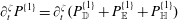 $\unicode[STIX]{x2202}_{t}^{\unicode[STIX]{x1D701}}P^{\{1\}}=\unicode[STIX]{x2202}_{t}^{\unicode[STIX]{x1D701}}(P_{\mathbb{D}}^{\{1\}}+P_{\mathbb{E}}^{\{1\}}+P_{\mathbb{H}}^{\{1\}})$
, correct to third order, because the time derivatives of
$\unicode[STIX]{x2202}_{t}^{\unicode[STIX]{x1D701}}P^{\{1\}}=\unicode[STIX]{x2202}_{t}^{\unicode[STIX]{x1D701}}(P_{\mathbb{D}}^{\{1\}}+P_{\mathbb{E}}^{\{1\}}+P_{\mathbb{H}}^{\{1\}})$
, correct to third order, because the time derivatives of
 $P_{\mathbb{A}}^{\{1\}}$
,
$P_{\mathbb{A}}^{\{1\}}$
,
 $P_{\mathbb{B}}^{\{1\}}$
,
$P_{\mathbb{B}}^{\{1\}}$
,
 $P_{\mathbb{C}}^{\{1\}}$
and
$P_{\mathbb{C}}^{\{1\}}$
and
 $P_{\mathbb{F}}^{\{1\}}$
are of fourth or higher order.
$P_{\mathbb{F}}^{\{1\}}$
are of fourth or higher order.Substituting the aforementioned pressure solutions and (D 2c ) into the upper boundary condition (B 6a ) yields (5.14) and (5.15). Then, (C 3)–(C 5), (5.11), (5.14), (5.15b ) and the scaling conditions (§ 3) yield
 $$\begin{eqnarray}\displaystyle & \displaystyle \unicode[STIX]{x2202}_{t}\unicode[STIX]{x2202}_{t}a=\frac{c^{[0]}a}{4}\unicode[STIX]{x2202}_{2}\unicode[STIX]{x2202}_{2}(\hat{k}_{1}u_{1}^{D}+c^{[2]})-\frac{1}{2}\unicode[STIX]{x2202}_{t}\,\text{Re}(G)+O(\unicode[STIX]{x1D716}^{4}{c^{[0]}}^{2}k), & \displaystyle\end{eqnarray}$$
 $$\begin{eqnarray}\displaystyle & \displaystyle \unicode[STIX]{x2202}_{t}c^{[2]}=\frac{c^{[0]}}{4ak^{2}}\left(\frac{a}{2}\unicode[STIX]{x2202}_{2}\unicode[STIX]{x2202}_{2}D^{g}+\frac{1}{2}\unicode[STIX]{x2202}_{2}\unicode[STIX]{x2202}_{2}\,\text{Re}(G)\right)-\frac{1}{2ak}\text{i}\unicode[STIX]{x2202}_{t}\,\text{Im}(G)+O(\unicode[STIX]{x1D716}^{3}{c^{[0]}}^{2}k), & \displaystyle\end{eqnarray}$$
 $$\begin{eqnarray}\displaystyle & \displaystyle \unicode[STIX]{x2202}_{t}\hat{k}_{1}=O(\unicode[STIX]{x1D716}^{3}c^{[0]}k), & \displaystyle\end{eqnarray}$$
 $$\begin{eqnarray}\displaystyle & \displaystyle \unicode[STIX]{x2202}_{t}\unicode[STIX]{x2202}_{t}\hat{k}_{2}=-\frac{c^{[0]}}{4ak^{2}}\left(\frac{a}{2}\unicode[STIX]{x2202}_{2}\unicode[STIX]{x2202}_{2}\unicode[STIX]{x2202}_{2}D^{g}+\frac{1}{2}\unicode[STIX]{x2202}_{2}\unicode[STIX]{x2202}_{2}\unicode[STIX]{x2202}_{2}\,\text{Re}(G)\right)+O(\unicode[STIX]{x1D716}^{3}{c^{[0]}}^{2}k^{2}). & \displaystyle\end{eqnarray}$$
Once the horizontal boundary condition (hence,
 $C_{(2)}$
,
$C_{(2)}$
,
 $C_{(n,3)}$
,
$C_{(n,3)}$
,
 $C_{(n,4)}$
and
$C_{(n,4)}$
and
 $K_{(n)}$
in (5.23a
)) and
$K_{(n)}$
in (5.23a
)) and
 $u_{1}^{c}+\mathfrak{U}_{1}$
are specified, then the derived solutions are fully determined. (Note that the accuracy of
$u_{1}^{c}+\mathfrak{U}_{1}$
are specified, then the derived solutions are fully determined. (Note that the accuracy of
 $u_{1}^{c}+\mathfrak{U}_{1}$
necessary for computing the third-order wave solutions is only
$u_{1}^{c}+\mathfrak{U}_{1}$
necessary for computing the third-order wave solutions is only
 $O(\unicode[STIX]{x1D716}^{2}c^{[0]})$
.)
$O(\unicode[STIX]{x1D716}^{2}c^{[0]})$
.)
The third-order, second- and third-harmonic solutions are
 $$\begin{eqnarray}\displaystyle & \displaystyle P^{\{2\}}=C_{(3)}\cos (\sqrt{12}ky+C_{(4)})\text{e}^{4k\unicode[STIX]{x1D701}}, & \displaystyle\end{eqnarray}$$
 $$\begin{eqnarray}\displaystyle & \displaystyle u^{\{2\}}=\frac{\hat{k}_{1}}{c^{[0]}}P^{\{2\}}, & \displaystyle\end{eqnarray}$$
 $$\begin{eqnarray}\displaystyle & \displaystyle v^{\{2\}}=\text{i}\frac{\sqrt{3}}{c^{[0]}}C_{(3)}\sin (\sqrt{12}ky+C_{(4)})\text{e}^{4k\unicode[STIX]{x1D701}}, & \displaystyle\end{eqnarray}$$
 $$\begin{eqnarray}\displaystyle & \displaystyle w^{\{2\}}=-\text{i}\frac{2}{c^{[0]}}P^{\{2\}}, & \displaystyle\end{eqnarray}$$
 $$\begin{eqnarray}\displaystyle & \displaystyle z^{\{2\}}=\frac{1}{g}P^{\{2\}}, & \displaystyle\end{eqnarray}$$
 $$\begin{eqnarray}\displaystyle & \displaystyle P^{\{3\}}={\textstyle \frac{3}{8}}{c^{[0]}}^{2}a^{3}k^{3}\text{e}^{3k\unicode[STIX]{x1D701}}+C_{(5)}\cos (\sqrt{72}ky+C_{(6)})\text{e}^{9k\unicode[STIX]{x1D701}}, & \displaystyle\end{eqnarray}$$
 $$\begin{eqnarray}\displaystyle & \displaystyle u^{\{3\}}=\frac{\hat{k}_{1}}{c^{[0]}}P^{\{3\}}, & \displaystyle\end{eqnarray}$$
 $$\begin{eqnarray}\displaystyle & \displaystyle v^{\{3\}}=\text{i}\frac{\sqrt{8}}{c^{[0]}}C_{(5)}\sin (\sqrt{72}\,ky+C_{(6)})\text{e}^{9k\unicode[STIX]{x1D701}}, & \displaystyle\end{eqnarray}$$
 $$\begin{eqnarray}\displaystyle & \displaystyle w^{\{3\}}=-\text{i}\frac{3}{8}c^{[0]}a^{3}k^{3}\text{e}^{3k\unicode[STIX]{x1D701}}-\text{i}\frac{3}{c^{[0]}}C_{(5)}\cos (\sqrt{72}ky+C_{(6)})\text{e}^{9k\unicode[STIX]{x1D701}}, & \displaystyle\end{eqnarray}$$
 $$\begin{eqnarray}\displaystyle & \displaystyle z^{\{3\}}=\frac{3}{8}a^{3}k^{2}\text{e}^{3k\unicode[STIX]{x1D701}}+\frac{1}{g}C_{(5)}\cos (\sqrt{72}ky+C_{(6)})\text{e}^{9k\unicode[STIX]{x1D701}}, & \displaystyle\end{eqnarray}$$
 $C_{(3)}$
and
$C_{(3)}$
and
 $C_{(5)}$
and real numbers
$C_{(5)}$
and real numbers
 $C_{(4)}$
and
$C_{(4)}$
and
 $C_{(6)}$
are constants to be determined by a full specification of the horizontal boundary condition. For simplicity, the solutions are obtained for a class of horizontal boundary conditions that change slowly enough so that scaling conditions
$C_{(6)}$
are constants to be determined by a full specification of the horizontal boundary condition. For simplicity, the solutions are obtained for a class of horizontal boundary conditions that change slowly enough so that scaling conditions
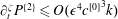 $\unicode[STIX]{x2202}_{t}^{\unicode[STIX]{x1D701}}P^{\{2\}}\leqslant O(\unicode[STIX]{x1D716}^{4}{c^{[0]}}^{3}k)$
and
$\unicode[STIX]{x2202}_{t}^{\unicode[STIX]{x1D701}}P^{\{2\}}\leqslant O(\unicode[STIX]{x1D716}^{4}{c^{[0]}}^{3}k)$
and
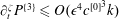 $\unicode[STIX]{x2202}_{t}^{\unicode[STIX]{x1D701}}P^{\{3\}}\leqslant O(\unicode[STIX]{x1D716}^{4}{c^{[0]}}^{3}k)$
are valid. (Because the governing equations for the second and third harmonics in appendix B contain no terms that require
$\unicode[STIX]{x2202}_{t}^{\unicode[STIX]{x1D701}}P^{\{3\}}\leqslant O(\unicode[STIX]{x1D716}^{4}{c^{[0]}}^{3}k)$
are valid. (Because the governing equations for the second and third harmonics in appendix B contain no terms that require
 $\unicode[STIX]{x2202}_{t}^{\unicode[STIX]{x1D701}}P^{\{2\}}$
and
$\unicode[STIX]{x2202}_{t}^{\unicode[STIX]{x1D701}}P^{\{2\}}$
and
 $\unicode[STIX]{x2202}_{t}^{\unicode[STIX]{x1D701}}P^{\{3\}}$
be non-zero to third order, these derivatives depend solely on the time dependence of the horizontal boundary condition.) These solutions are derived in the following way. Combining (B 1d
), (B 1e
), (B 1f
), (B 2b
) and (B 3b
) yields
$\unicode[STIX]{x2202}_{t}^{\unicode[STIX]{x1D701}}P^{\{3\}}$
be non-zero to third order, these derivatives depend solely on the time dependence of the horizontal boundary condition.) These solutions are derived in the following way. Combining (B 1d
), (B 1e
), (B 1f
), (B 2b
) and (B 3b
) yields
 $(\unicode[STIX]{x2202}_{2}^{\unicode[STIX]{x1D701}}\unicode[STIX]{x2202}_{2}^{\unicode[STIX]{x1D701}}+\unicode[STIX]{x2202}_{3}^{\unicode[STIX]{x1D701}}\unicode[STIX]{x2202}_{3}^{\unicode[STIX]{x1D701}}-4k^{2})P^{\{2\}}=O(\unicode[STIX]{x1D716}^{4}{c^{[0]}}^{2}k^{2})$
with the boundary conditions (B 5) and (B 6b
). Likewise, combining (B 1g
), (B 1h
), (B 1i
), (B 2c
) and (B 3c
) yields
$(\unicode[STIX]{x2202}_{2}^{\unicode[STIX]{x1D701}}\unicode[STIX]{x2202}_{2}^{\unicode[STIX]{x1D701}}+\unicode[STIX]{x2202}_{3}^{\unicode[STIX]{x1D701}}\unicode[STIX]{x2202}_{3}^{\unicode[STIX]{x1D701}}-4k^{2})P^{\{2\}}=O(\unicode[STIX]{x1D716}^{4}{c^{[0]}}^{2}k^{2})$
with the boundary conditions (B 5) and (B 6b
). Likewise, combining (B 1g
), (B 1h
), (B 1i
), (B 2c
) and (B 3c
) yields
 $(\unicode[STIX]{x2202}_{2}^{\unicode[STIX]{x1D701}}\unicode[STIX]{x2202}_{2}^{\unicode[STIX]{x1D701}}+\unicode[STIX]{x2202}_{3}^{\unicode[STIX]{x1D701}}\unicode[STIX]{x2202}_{3}^{\unicode[STIX]{x1D701}}-9k^{2})P^{\{3\}}=O(\unicode[STIX]{x1D716}^{4}{c^{[0]}}^{2}k^{2})$
with the boundary conditions (B 5) and (B 6c
). The other solutions follow directly from (B 1d
), (B 1e
), (B 1f
), (B 7b
), (B 1g
), (B 1h
), (B 1i
) and (B 7c
).
$(\unicode[STIX]{x2202}_{2}^{\unicode[STIX]{x1D701}}\unicode[STIX]{x2202}_{2}^{\unicode[STIX]{x1D701}}+\unicode[STIX]{x2202}_{3}^{\unicode[STIX]{x1D701}}\unicode[STIX]{x2202}_{3}^{\unicode[STIX]{x1D701}}-9k^{2})P^{\{3\}}=O(\unicode[STIX]{x1D716}^{4}{c^{[0]}}^{2}k^{2})$
with the boundary conditions (B 5) and (B 6c
). The other solutions follow directly from (B 1d
), (B 1e
), (B 1f
), (B 7b
), (B 1g
), (B 1h
), (B 1i
) and (B 7c
).Appendix E. Solutions of
$S_{i}$

Equations (5.7d
), (5.9d
), (5.10) and equations
 $ak=O(\unicode[STIX]{x1D716})$
and
$ak=O(\unicode[STIX]{x1D716})$
and
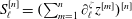 $S_{\ell }^{[n]}=(\sum _{m=1}^{n}\unicode[STIX]{x2202}_{\ell }^{\unicode[STIX]{x1D701}}z^{[m]})^{[n]}$
yield the following solutions for
$S_{\ell }^{[n]}=(\sum _{m=1}^{n}\unicode[STIX]{x2202}_{\ell }^{\unicode[STIX]{x1D701}}z^{[m]})^{[n]}$
yield the following solutions for
 $S_{i}$
:
$S_{i}$
:
 $S_{i}^{[0]}=0$
,
$S_{i}^{[0]}=0$
,
 $S_{h}^{[1]}=-\hat{k}_{h}ak\text{e}^{k\unicode[STIX]{x1D701}}\sin \unicode[STIX]{x1D712}$
,
$S_{h}^{[1]}=-\hat{k}_{h}ak\text{e}^{k\unicode[STIX]{x1D701}}\sin \unicode[STIX]{x1D712}$
,
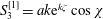 $S_{3}^{[1]}=ak\text{e}^{k\unicode[STIX]{x1D701}}\cos \unicode[STIX]{x1D712}$
,
$S_{3}^{[1]}=ak\text{e}^{k\unicode[STIX]{x1D701}}\cos \unicode[STIX]{x1D712}$
,
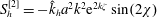 $S_{h}^{[2]}=-\hat{k}_{h}a^{2}k^{2}\text{e}^{2k\unicode[STIX]{x1D701}}\sin (2\unicode[STIX]{x1D712})$
,
$S_{h}^{[2]}=-\hat{k}_{h}a^{2}k^{2}\text{e}^{2k\unicode[STIX]{x1D701}}\sin (2\unicode[STIX]{x1D712})$
,
 $S_{3}^{[2]}=a^{2}k^{2}\text{e}^{2k\unicode[STIX]{x1D701}}\cos (2\unicode[STIX]{x1D712})$
and
$S_{3}^{[2]}=a^{2}k^{2}\text{e}^{2k\unicode[STIX]{x1D701}}\cos (2\unicode[STIX]{x1D712})$
and
 $$\begin{eqnarray}\left.\begin{array}{@{}c@{}}\displaystyle \begin{array}{@{}rcl@{}}\displaystyle S_{h}^{[3]}\; & =\; & \displaystyle \unicode[STIX]{x2202}_{h}^{\unicode[STIX]{x1D701}}(a\text{e}^{k\unicode[STIX]{x1D701}})\cos \unicode[STIX]{x1D712}+\mathop{\sum }_{m=1}^{3}[\unicode[STIX]{x2202}_{h}^{\unicode[STIX]{x1D701}}\,\text{Re}(z^{\{m\}})+\text{i}m\hat{k}_{h}k\,\text{Im}(z^{\{m\}})]\cos (m\unicode[STIX]{x1D712})\\ \; & \; & +\,\displaystyle \mathop{\sum }_{m=1}^{3}[\text{i}\unicode[STIX]{x2202}_{h}^{\unicode[STIX]{x1D701}}\,\text{Im}(z^{\{m\}})-m\hat{k}_{h}k\,\text{Re}(z^{\{m\}})]\sin (m\unicode[STIX]{x1D712}),\end{array}\\ \displaystyle S_{3}^{[3]}=\mathop{\sum }_{m=1}^{3}[\unicode[STIX]{x2202}_{3}^{\unicode[STIX]{x1D701}}\,\text{Re}(z^{\{m\}})]\cos (m\unicode[STIX]{x1D712})+\mathop{\sum }_{m=1}^{3}[\text{i}\unicode[STIX]{x2202}_{3}^{\unicode[STIX]{x1D701}}\,\text{Im}(z^{\{m\}})]\sin (m\unicode[STIX]{x1D712}).\end{array}\right\}\end{eqnarray}$$
The solutions of
 $z^{\{m\}}$
are given in (D 2d
), (D 4e
) and (D 5e
).
$z^{\{m\}}$
are given in (D 2d
), (D 4e
) and (D 5e
).
Appendix F. Solutions of
$\langle S_{3}u_{h}^{w}\rangle$
and
$\langle S_{h}u_{h}^{w}\rangle$


These are
 $$\begin{eqnarray}\displaystyle \langle S_{3}u_{1}^{w}\rangle & = & \displaystyle \langle S_{3}^{[1]}{u_{1}^{w}}^{[1]}\rangle +\langle S_{3}^{[1]}{u_{1}^{w}}^{[3]}\rangle +\langle S_{3}^{[2]}{u_{1}^{w}}^{[2]}\rangle +\langle S_{3}^{[3]}{u_{1}^{w}}^{[1]}\rangle +O(\unicode[STIX]{x1D716}^{5}c^{[0]})\nonumber\\ \displaystyle & = & \displaystyle \frac{1}{2}U_{1}^{S}+\frac{13}{8}\hat{k}_{1}c^{[0]}a^{4}k^{4}\text{e}^{4k\unicode[STIX]{x1D701}}+\frac{\hat{k}_{1}ak}{2c^{[0]}}\text{e}^{k\unicode[STIX]{x1D701}}\left(\,\text{Re}(P^{\{1\}})+\frac{1}{k^{2}}\unicode[STIX]{x2202}_{3}^{\unicode[STIX]{x1D701}}\unicode[STIX]{x2202}_{3}^{\unicode[STIX]{x1D701}}\,\text{Re}(P^{\{1\}})\right)\nonumber\\ \displaystyle & & \displaystyle +\,\frac{\hat{k}_{1}a}{2{c^{[0]}}^{2}}\text{e}^{k\unicode[STIX]{x1D701}}\left(-\text{i}\unicode[STIX]{x2202}_{t}^{\unicode[STIX]{x1D701}}\,\text{Im}(P^{\{1\}})-\frac{2}{k^{2}}\text{i}\unicode[STIX]{x2202}_{3}^{\unicode[STIX]{x1D701}}\unicode[STIX]{x2202}_{3}^{\unicode[STIX]{x1D701}}\unicode[STIX]{x2202}_{t}^{\unicode[STIX]{x1D701}}\,\text{Im}(P^{\{1\}})-4c^{[0]}\text{e}^{k\unicode[STIX]{x1D701}}\unicode[STIX]{x2202}_{t}\unicode[STIX]{x2202}_{t}a\right)\nonumber\\ \displaystyle & & \displaystyle +\,\frac{3}{2}a^{2}k^{2}\text{e}^{2k\unicode[STIX]{x1D701}}(u_{1}^{c}-u_{1}^{D}+\mathfrak{U}_{1}-c^{[2]}\hat{k}_{1})+a^{2}k\text{e}^{2k\unicode[STIX]{x1D701}}\unicode[STIX]{x2202}_{3}^{\unicode[STIX]{x1D701}}(u_{1}^{c}+\mathfrak{U}_{1})+O(\unicode[STIX]{x1D716}^{5}c^{[0]}),\qquad\end{eqnarray}$$
 $$\begin{eqnarray}\displaystyle \langle S_{3}u_{2}^{w}\rangle & = & \displaystyle \langle S_{3}^{[1]}{u_{2}^{w}}^{[1]}\rangle +\langle S_{3}^{[1]}{u_{2}^{w}}^{[3]}\rangle +\langle S_{3}^{[2]}{u_{2}^{w}}^{[2]}\rangle +\langle S_{3}^{[3]}{u_{2}^{w}}^{[1]}\rangle +O(\unicode[STIX]{x1D716}^{5}c^{[0]})\nonumber\\ \displaystyle & = & \displaystyle \frac{1}{2}U_{2}^{S}-\frac{a^{2}}{2c^{[0]}}\text{e}^{2k\unicode[STIX]{x1D701}}\unicode[STIX]{x2202}_{t}\unicode[STIX]{x2202}_{t}\hat{k}_{2}\nonumber\\ \displaystyle & & \displaystyle +\,\frac{a}{2}\text{e}^{k\unicode[STIX]{x1D701}}\left(-\frac{1}{g}\unicode[STIX]{x2202}_{2}^{\unicode[STIX]{x1D701}}\unicode[STIX]{x2202}_{t}^{\unicode[STIX]{x1D701}}\,\text{Re}(P^{\{1\}})-\frac{1}{c^{[0]}}\text{i}\unicode[STIX]{x2202}_{2}^{\unicode[STIX]{x1D701}}\,\text{Im}(P^{\{1\}})-\text{e}^{k\unicode[STIX]{x1D701}}\unicode[STIX]{x2202}_{2}\unicode[STIX]{x2202}_{t}a\right)+O(\unicode[STIX]{x1D716}^{5}c^{[0]}),\qquad\end{eqnarray}$$
 $$\begin{eqnarray}\displaystyle -\langle S_{h}u_{h}^{w}\rangle & = & \displaystyle -\langle S_{h}^{[1]}{u_{h}^{w}}^{[3]}\rangle -\langle S_{h}^{[3]}{u_{h}^{w}}^{[1]}\rangle +O(\unicode[STIX]{x1D716}^{5}c^{[0]})\nonumber\\ \displaystyle & = & \displaystyle -\frac{1}{2}ak\text{e}^{k\unicode[STIX]{x1D701}}\unicode[STIX]{x2202}_{t}^{\unicode[STIX]{x1D701}}(a\text{e}^{k\unicode[STIX]{x1D701}})+\frac{a}{2{c^{[0]}}^{2}}\text{e}^{k\unicode[STIX]{x1D701}}\left(\unicode[STIX]{x2202}_{t}^{\unicode[STIX]{x1D701}}\,\text{Re}(P^{\{1\}})-\frac{2}{k}\unicode[STIX]{x2202}_{3}^{\unicode[STIX]{x1D701}}\unicode[STIX]{x2202}_{t}^{\unicode[STIX]{x1D701}}\,\text{Re}(P^{\{1\}})\right)\nonumber\\ \displaystyle & & \displaystyle +\,\frac{ak}{2c^{[0]}}\text{e}^{k\unicode[STIX]{x1D701}}\left(\text{i}\,\text{Im}(P^{\{1\}})-\frac{1}{k}\text{i}\unicode[STIX]{x2202}_{3}^{\unicode[STIX]{x1D701}}\,\text{Im}(P^{\{1\}})+2a\text{e}^{k\unicode[STIX]{x1D701}}\unicode[STIX]{x2202}_{t}c^{[2]}\right)+O(\unicode[STIX]{x1D716}^{5}c^{[0]}).\qquad\end{eqnarray}$$
Appendix G. Pseudo-incompressibility of other flows
The ensemble-averaged flow
 $\langle \boldsymbol{u}\rangle$
does not satisfy its pseudo-incompressibility to the necessary (i.e. fourth-order) accuracy. In fact, (2.5) and (6.3)–(6.4c
) yield
$\langle \boldsymbol{u}\rangle$
does not satisfy its pseudo-incompressibility to the necessary (i.e. fourth-order) accuracy. In fact, (2.5) and (6.3)–(6.4c
) yield
 $$\begin{eqnarray}\unicode[STIX]{x2202}_{i}^{\unicode[STIX]{x1D701}}\langle u_{i}\rangle =-\unicode[STIX]{x2202}_{h}^{\unicode[STIX]{x1D701}}\langle S_{3}u_{h}\rangle +\unicode[STIX]{x2202}_{3}^{\unicode[STIX]{x1D701}}\langle S_{h}u_{h}\rangle .\end{eqnarray}$$
Meanwhile,
 $\langle S_{3}u_{h}\rangle =\langle S_{3}u_{h}^{w}\rangle +O(\unicode[STIX]{x1D716}^{5}c^{[0]})$
and
$\langle S_{3}u_{h}\rangle =\langle S_{3}u_{h}^{w}\rangle +O(\unicode[STIX]{x1D716}^{5}c^{[0]})$
and
 $\langle S_{h}u_{h}\rangle =\langle S_{h}u_{h}^{w}\rangle +O(\unicode[STIX]{x1D716}^{5}c^{[0]})$
according to (3.1) and appendix E. Therefore, the right-hand side of (G 1) can be computed from (F 1)–(F 3). The result shows that
$\langle S_{h}u_{h}\rangle =\langle S_{h}u_{h}^{w}\rangle +O(\unicode[STIX]{x1D716}^{5}c^{[0]})$
according to (3.1) and appendix E. Therefore, the right-hand side of (G 1) can be computed from (F 1)–(F 3). The result shows that
 $\unicode[STIX]{x2202}_{i}^{\unicode[STIX]{x1D701}}\langle u_{i}\rangle$
is of fourth order. In terms of the Poisson equation, we must consider
$\unicode[STIX]{x2202}_{i}^{\unicode[STIX]{x1D701}}\langle u_{i}\rangle$
is of fourth order. In terms of the Poisson equation, we must consider
 $\unicode[STIX]{x2202}_{i}^{\unicode[STIX]{x1D701}}\unicode[STIX]{x2202}_{t}^{\unicode[STIX]{x1D701}}\langle u_{i}\rangle$
. According to (F 1)–(F 3) and the scaling conditions in § 3, we have
$\unicode[STIX]{x2202}_{i}^{\unicode[STIX]{x1D701}}\unicode[STIX]{x2202}_{t}^{\unicode[STIX]{x1D701}}\langle u_{i}\rangle$
. According to (F 1)–(F 3) and the scaling conditions in § 3, we have
 $$\begin{eqnarray}\displaystyle \unicode[STIX]{x2202}_{t}^{\unicode[STIX]{x1D701}}\langle S_{3}u_{1}\rangle & = & \displaystyle \frac{1}{2}\unicode[STIX]{x2202}_{t}^{\unicode[STIX]{x1D701}}U_{1}^{S}-\frac{3}{2}a^{2}k^{2}\text{e}^{2k\unicode[STIX]{x1D701}}\hat{k}_{1}\unicode[STIX]{x2202}_{t}c^{[2]}\nonumber\\ \displaystyle & & \displaystyle +\,\frac{\hat{k}_{1}ak}{2c^{[0]}}\text{e}^{k\unicode[STIX]{x1D701}}\left(\unicode[STIX]{x2202}_{t}^{\unicode[STIX]{x1D701}}\,\text{Re}(P^{\{1\}})+\frac{1}{k^{2}}\unicode[STIX]{x2202}_{3}^{\unicode[STIX]{x1D701}}\unicode[STIX]{x2202}_{3}^{\unicode[STIX]{x1D701}}\unicode[STIX]{x2202}_{t}^{\unicode[STIX]{x1D701}}\,\text{Re}(P^{\{1\}})\right)+O(\unicode[STIX]{x1D716}^{5}{c^{[0]}}^{2}k),\end{eqnarray}$$
 $$\begin{eqnarray}\displaystyle & \displaystyle \unicode[STIX]{x2202}_{t}^{\unicode[STIX]{x1D701}}\langle S_{3}u_{2}\rangle =\frac{1}{2}\unicode[STIX]{x2202}_{t}^{\unicode[STIX]{x1D701}}U_{2}^{S}-\frac{a}{2}\text{e}^{k\unicode[STIX]{x1D701}}\left(\frac{1}{c^{[0]}}\text{i}\unicode[STIX]{x2202}_{2}^{\unicode[STIX]{x1D701}}\unicode[STIX]{x2202}_{t}^{\unicode[STIX]{x1D701}}\,\text{Im}(P^{\{1\}})+\text{e}^{k\unicode[STIX]{x1D701}}\unicode[STIX]{x2202}_{2}\unicode[STIX]{x2202}_{t}\unicode[STIX]{x2202}_{t}a\right)+O(\unicode[STIX]{x1D716}^{5}{c^{[0]}}^{2}k), & \displaystyle\end{eqnarray}$$
 $$\begin{eqnarray}\displaystyle -\unicode[STIX]{x2202}_{t}^{\unicode[STIX]{x1D701}}\langle S_{h}u_{h}\rangle & = & \displaystyle -\frac{ak}{2}\text{e}^{2k\unicode[STIX]{x1D701}}\unicode[STIX]{x2202}_{t}\unicode[STIX]{x2202}_{t}a\nonumber\\ \displaystyle & & \displaystyle +\,\frac{ak}{2c^{[0]}}\text{e}^{k\unicode[STIX]{x1D701}}\left(\text{i}\unicode[STIX]{x2202}_{t}^{\unicode[STIX]{x1D701}}\,\text{Im}(P^{\{1\}})-\frac{1}{k}\text{i}\unicode[STIX]{x2202}_{3}^{\unicode[STIX]{x1D701}}\unicode[STIX]{x2202}_{t}^{\unicode[STIX]{x1D701}}\,\text{Im}(P^{\{1\}})\right)+O(\unicode[STIX]{x1D716}^{5}{c^{[0]}}^{2}k).\end{eqnarray}$$
Then, (D 3a ), (G 1)–(G 4) and the scaling conditions in § 3 yield
 $$\begin{eqnarray}\unicode[STIX]{x2202}_{i}^{\unicode[STIX]{x1D701}}\unicode[STIX]{x2202}_{t}^{\unicode[STIX]{x1D701}}\langle u_{i}\rangle =ak^{2}\text{e}^{2k\unicode[STIX]{x1D701}}\left(\frac{c^{[0]}a}{4}\unicode[STIX]{x2202}_{2}\unicode[STIX]{x2202}_{2}(\hat{k}_{1}u_{1}^{D}+c^{[2]})-\frac{1}{2}\unicode[STIX]{x2202}_{t}\,\text{Re}(G)\right)+O(\unicode[STIX]{x1D716}^{5}{c^{[0]}}^{2}k^{2}).\end{eqnarray}$$
The right-hand side of (G 5) is of fourth order.
The ensemble-averaged current
 $\langle \boldsymbol{u}^{c}\rangle$
is not guaranteed to satisfy its pseudo-incompressibility. According to (6.3), we have
$\langle \boldsymbol{u}^{c}\rangle$
is not guaranteed to satisfy its pseudo-incompressibility. According to (6.3), we have
 $\unicode[STIX]{x2202}_{i}^{\unicode[STIX]{x1D701}}\langle u_{i}^{c}\rangle =-\unicode[STIX]{x2202}_{i}^{\unicode[STIX]{x1D701}}\mathfrak{U}_{i}-\unicode[STIX]{x2202}_{h}^{\unicode[STIX]{x1D701}}\langle S_{3}u_{h}\rangle +\unicode[STIX]{x2202}_{3}^{\unicode[STIX]{x1D701}}\langle S_{h}u_{h}\rangle$
. There is no reason to assume that the right-hand side of this equation is negligible to fourth order.
$\unicode[STIX]{x2202}_{i}^{\unicode[STIX]{x1D701}}\langle u_{i}^{c}\rangle =-\unicode[STIX]{x2202}_{i}^{\unicode[STIX]{x1D701}}\mathfrak{U}_{i}-\unicode[STIX]{x2202}_{h}^{\unicode[STIX]{x1D701}}\langle S_{3}u_{h}\rangle +\unicode[STIX]{x2202}_{3}^{\unicode[STIX]{x1D701}}\langle S_{h}u_{h}\rangle$
. There is no reason to assume that the right-hand side of this equation is negligible to fourth order.
The quasi-current
 $\boldsymbol{u}^{Q}\equiv (\langle u_{h}\rangle -U_{h}^{S}/2,\langle w\rangle )$
does not satisfy pseudo-incompressibility. In fact, according to (5.50), (G 1), (G 5) and the scaling conditions in § 3, both
$\boldsymbol{u}^{Q}\equiv (\langle u_{h}\rangle -U_{h}^{S}/2,\langle w\rangle )$
does not satisfy pseudo-incompressibility. In fact, according to (5.50), (G 1), (G 5) and the scaling conditions in § 3, both
 $\unicode[STIX]{x2202}_{i}^{\unicode[STIX]{x1D701}}u_{i}^{Q}$
and
$\unicode[STIX]{x2202}_{i}^{\unicode[STIX]{x1D701}}u_{i}^{Q}$
and
 $\unicode[STIX]{x2202}_{i}^{\unicode[STIX]{x1D701}}\unicode[STIX]{x2202}_{t}^{\unicode[STIX]{x1D701}}u_{i}^{Q}$
are of fourth order.
$\unicode[STIX]{x2202}_{i}^{\unicode[STIX]{x1D701}}\unicode[STIX]{x2202}_{t}^{\unicode[STIX]{x1D701}}u_{i}^{Q}$
are of fourth order.
Appendix H. Derivation of (6.5)
Averaging (5.1) using (2.5) and combining it with (5.50) and the identities in appendix C yields the following momentum equations:
 $$\begin{eqnarray}\displaystyle & & \displaystyle (\unicode[STIX]{x2202}_{t}^{\unicode[STIX]{x1D701}}+\langle u_{H}\rangle \unicode[STIX]{x2202}_{H}^{\unicode[STIX]{x1D701}}+\langle w^{c}\rangle \unicode[STIX]{x2202}_{3}^{\unicode[STIX]{x1D701}})\left(\langle u_{1}\rangle -{\textstyle \frac{1}{2}}U_{1}^{S}\right)+\unicode[STIX]{x2202}_{1}^{\unicode[STIX]{x1D701}}\langle P^{[4]}\rangle +\unicode[STIX]{x2202}_{1}^{\unicode[STIX]{x1D701}}\left(\unicode[STIX]{x1D6F7}-{\textstyle \frac{1}{4}}U_{H}^{S}U_{H}^{S}\right)\nonumber\\ \displaystyle & & \displaystyle \quad -\,\frac{a}{c^{[0]}}\text{e}^{k\unicode[STIX]{x1D701}}\hat{k}_{1}\unicode[STIX]{x2202}_{3}^{\unicode[STIX]{x1D701}}\unicode[STIX]{x2202}_{t}^{\unicode[STIX]{x1D701}}\,\text{Re}(P^{\{1\}})+{\textstyle \frac{3}{2}}a^{2}k^{2}\text{e}^{2k\unicode[STIX]{x1D701}}\hat{k}_{1}\unicode[STIX]{x2202}_{t}c^{[2]}=O(\unicode[STIX]{x1D716}^{5}{c^{[0]}}^{2}k),\end{eqnarray}$$
 $$\begin{eqnarray}\displaystyle & & \displaystyle (\unicode[STIX]{x2202}_{t}^{\unicode[STIX]{x1D701}}+\langle u_{H}\rangle \unicode[STIX]{x2202}_{H}^{\unicode[STIX]{x1D701}}+\langle w^{c}\rangle \unicode[STIX]{x2202}_{3}^{\unicode[STIX]{x1D701}})(\langle u_{2}\rangle -{\textstyle \frac{1}{2}}U_{2}^{S})+\unicode[STIX]{x2202}_{2}^{\unicode[STIX]{x1D701}}\langle P^{[4]}\rangle +\unicode[STIX]{x2202}_{2}^{\unicode[STIX]{x1D701}}(\unicode[STIX]{x1D6F7}-{\textstyle \frac{1}{4}}U_{H}^{S}U_{H}^{S})\nonumber\\ \displaystyle & & \displaystyle \quad -\,U_{1}^{S}\unicode[STIX]{x2202}_{2}^{\unicode[STIX]{x1D701}}(\langle u_{1}\rangle -{\textstyle \frac{1}{2}}U_{1}^{S})=O(\unicode[STIX]{x1D716}^{5}{c^{[0]}}^{2}k),\end{eqnarray}$$
 $$\begin{eqnarray}\displaystyle & & \displaystyle (\unicode[STIX]{x2202}_{t}^{\unicode[STIX]{x1D701}}+\langle u_{H}\rangle \unicode[STIX]{x2202}_{H}^{\unicode[STIX]{x1D701}}+\langle w^{c}\rangle \unicode[STIX]{x2202}_{3}^{\unicode[STIX]{x1D701}})\langle w\rangle +\unicode[STIX]{x2202}_{3}^{\unicode[STIX]{x1D701}}\langle P^{[4]}\rangle +\unicode[STIX]{x2202}_{3}^{\unicode[STIX]{x1D701}}\left(\unicode[STIX]{x1D6F7}-{\textstyle \frac{1}{4}}U_{H}^{S}U_{H}^{S}\right)\nonumber\\ \displaystyle & & \displaystyle \quad -\,U_{1}^{S}\unicode[STIX]{x2202}_{3}^{\unicode[STIX]{x1D701}}\left(\langle u_{1}\rangle -{\textstyle \frac{1}{2}}U_{1}^{S}\right)-\frac{a}{c^{[0]}}\text{e}^{k\unicode[STIX]{x1D701}}\text{i}\unicode[STIX]{x2202}_{3}^{\unicode[STIX]{x1D701}}\unicode[STIX]{x2202}_{t}^{\unicode[STIX]{x1D701}}\,\text{Im}(P^{\{1\}})\nonumber\\ \displaystyle & & \displaystyle \quad -\,{\textstyle \frac{3}{2}}ak\text{e}^{2k\unicode[STIX]{x1D701}}\unicode[STIX]{x2202}_{t}\unicode[STIX]{x2202}_{t}a=O(\unicode[STIX]{x1D716}^{5}{c^{[0]}}^{2}k),\end{eqnarray}$$
 $\unicode[STIX]{x1D6F7}$
is defined by (6.5d
). The terms
$\unicode[STIX]{x1D6F7}$
is defined by (6.5d
). The terms
 $\langle u_{H}\rangle \unicode[STIX]{x2202}_{H}^{\unicode[STIX]{x1D701}}U_{h}^{S}$
and
$\langle u_{H}\rangle \unicode[STIX]{x2202}_{H}^{\unicode[STIX]{x1D701}}U_{h}^{S}$
and
 $\unicode[STIX]{x2202}_{1}^{\unicode[STIX]{x1D701}}\unicode[STIX]{x1D6F7}$
are of fifth order, and
$\unicode[STIX]{x2202}_{1}^{\unicode[STIX]{x1D701}}\unicode[STIX]{x1D6F7}$
are of fifth order, and
 $U_{H}^{S}\unicode[STIX]{x2202}_{h}^{\unicode[STIX]{x1D701}}U_{H}^{S}$
is of sixth order, according to the scaling conditions (§ 3) and the derived wave dynamics (§ 5). Without loss of generality, these terms are included in these equations because the properties of these equations become clearer in this way; e.g. the inclusion of
$U_{H}^{S}\unicode[STIX]{x2202}_{h}^{\unicode[STIX]{x1D701}}U_{H}^{S}$
is of sixth order, according to the scaling conditions (§ 3) and the derived wave dynamics (§ 5). Without loss of generality, these terms are included in these equations because the properties of these equations become clearer in this way; e.g. the inclusion of
 $\unicode[STIX]{x2202}_{1}^{\unicode[STIX]{x1D701}}\unicode[STIX]{x1D6F7}$
makes it clearer to see that
$\unicode[STIX]{x2202}_{1}^{\unicode[STIX]{x1D701}}\unicode[STIX]{x1D6F7}$
makes it clearer to see that
 $\unicode[STIX]{x2202}_{i}^{\unicode[STIX]{x1D701}}\unicode[STIX]{x1D6F7}$
is a potential force. Note that the terms
$\unicode[STIX]{x2202}_{i}^{\unicode[STIX]{x1D701}}\unicode[STIX]{x1D6F7}$
is a potential force. Note that the terms
 $-\unicode[STIX]{x2202}_{t}^{\unicode[STIX]{x1D701}}U_{h}^{S}/2$
(together with some other terms) derive from
$-\unicode[STIX]{x2202}_{t}^{\unicode[STIX]{x1D701}}U_{h}^{S}/2$
(together with some other terms) derive from
 $\langle {u_{H}^{w}}^{[1]}\unicode[STIX]{x2202}_{H}^{\unicode[STIX]{x1D701}}{u_{h}^{w}}^{[1]}\rangle$
,
$\langle {u_{H}^{w}}^{[1]}\unicode[STIX]{x2202}_{H}^{\unicode[STIX]{x1D701}}{u_{h}^{w}}^{[1]}\rangle$
,
 $\langle {u_{H}^{w}}^{[1]}\unicode[STIX]{x2202}_{H}^{\unicode[STIX]{x1D701}}{u_{h}^{w}}^{[3]}\rangle$
and
$\langle {u_{H}^{w}}^{[1]}\unicode[STIX]{x2202}_{H}^{\unicode[STIX]{x1D701}}{u_{h}^{w}}^{[3]}\rangle$
and
 $\langle -S_{h}^{[3]}\unicode[STIX]{x2202}_{3}^{\unicode[STIX]{x1D701}}P^{[1]}\rangle$
shown in table 2. Because
$\langle -S_{h}^{[3]}\unicode[STIX]{x2202}_{3}^{\unicode[STIX]{x1D701}}P^{[1]}\rangle$
shown in table 2. Because
 $\boldsymbol{u}^{Q}\equiv (\langle u_{h}\rangle -U_{h}^{S}/2,\langle w\rangle )$
is not pseudo-incompressible (appendix G), these equations do not form a solvable Poisson equation for the wave-averaged pressure
$\boldsymbol{u}^{Q}\equiv (\langle u_{h}\rangle -U_{h}^{S}/2,\langle w\rangle )$
is not pseudo-incompressible (appendix G), these equations do not form a solvable Poisson equation for the wave-averaged pressure
 $\langle P^{[4]}\rangle$
.
$\langle P^{[4]}\rangle$
.According to (6.4) and appendix F, we have
 $U_{h}=\langle u_{h}\rangle +\frac{1}{2}U_{h}^{S}+O(\unicode[STIX]{x1D716}^{4}c^{[0]})$
and
$U_{h}=\langle u_{h}\rangle +\frac{1}{2}U_{h}^{S}+O(\unicode[STIX]{x1D716}^{4}c^{[0]})$
and
 $W=\langle w^{c}\rangle +O(\unicode[STIX]{x1D716}^{4}c^{[0]})$
. These facts and the scaling conditions (§ 3) imply that
$W=\langle w^{c}\rangle +O(\unicode[STIX]{x1D716}^{4}c^{[0]})$
. These facts and the scaling conditions (§ 3) imply that
 $\langle u_{H}\rangle \unicode[STIX]{x2202}_{H}^{\unicode[STIX]{x1D701}}\langle u_{i}\rangle =U_{H}\unicode[STIX]{x2202}_{H}^{\unicode[STIX]{x1D701}}\langle u_{i}\rangle +O(\unicode[STIX]{x1D716}^{5}{c^{[0]}}^{2}k)$
and
$\langle u_{H}\rangle \unicode[STIX]{x2202}_{H}^{\unicode[STIX]{x1D701}}\langle u_{i}\rangle =U_{H}\unicode[STIX]{x2202}_{H}^{\unicode[STIX]{x1D701}}\langle u_{i}\rangle +O(\unicode[STIX]{x1D716}^{5}{c^{[0]}}^{2}k)$
and
 $U_{H}^{S}\unicode[STIX]{x2202}_{H}^{\unicode[STIX]{x1D701}}U_{h}^{S}\leqslant O(\unicode[STIX]{x1D716}^{6}{c^{[0]}}^{2}k)$
. Combining these equations with (5.50), (6.4), (G 2)–(G 4) and (H 1a
)–(H 1c
) yields (6.5).
$U_{H}^{S}\unicode[STIX]{x2202}_{H}^{\unicode[STIX]{x1D701}}U_{h}^{S}\leqslant O(\unicode[STIX]{x1D716}^{6}{c^{[0]}}^{2}k)$
. Combining these equations with (5.50), (6.4), (G 2)–(G 4) and (H 1a
)–(H 1c
) yields (6.5).
Appendix I. The vortex force form of (6.5)
We have
 $$\begin{eqnarray}\displaystyle & & \displaystyle \unicode[STIX]{x2202}_{t}^{\unicode[STIX]{x1D701}}U_{1}+(U_{H}\unicode[STIX]{x2202}_{H}^{\unicode[STIX]{x1D701}}+W\unicode[STIX]{x2202}_{3}^{\unicode[STIX]{x1D701}})(U_{1}-U_{1}^{S})+\unicode[STIX]{x2202}_{1}^{\unicode[STIX]{x1D701}}\langle P^{[4]}\rangle +\unicode[STIX]{x2202}_{1}^{\unicode[STIX]{x1D701}}(\unicode[STIX]{x1D6F7}+\unicode[STIX]{x1D719}+{\textstyle \frac{1}{4}}U_{H}^{S}U_{H}^{S})\nonumber\\ \displaystyle & & \displaystyle \quad -\,\unicode[STIX]{x2202}_{t}^{\unicode[STIX]{x1D701}}U_{1}^{S}+\unicode[STIX]{x1D6EC}_{1}=O(\unicode[STIX]{x1D716}^{5}{c^{[0]}}^{2}k),\end{eqnarray}$$
 $$\begin{eqnarray}\displaystyle & & \displaystyle \unicode[STIX]{x2202}_{t}^{\unicode[STIX]{x1D701}}U_{2}+(U_{H}\unicode[STIX]{x2202}_{H}^{\unicode[STIX]{x1D701}}+W\unicode[STIX]{x2202}_{3}^{\unicode[STIX]{x1D701}})(U_{2}-U_{2}^{S})+\unicode[STIX]{x2202}_{2}^{\unicode[STIX]{x1D701}}\langle P^{[4]}\rangle +\unicode[STIX]{x2202}_{2}^{\unicode[STIX]{x1D701}}(\unicode[STIX]{x1D6F7}+\unicode[STIX]{x1D719}+{\textstyle \frac{1}{4}}U_{H}^{S}U_{H}^{S})\nonumber\\ \displaystyle & & \displaystyle \quad +\,c_{H}^{g}\unicode[STIX]{x2202}_{H}^{\unicode[STIX]{x1D701}}U_{2}^{S}-U_{1}^{S}\unicode[STIX]{x2202}_{2}^{\unicode[STIX]{x1D701}}(U_{1}-u_{1}^{D}-c^{[2]}\hat{k}_{1})=O(\unicode[STIX]{x1D716}^{5}{c^{[0]}}^{2}k),\end{eqnarray}$$
 $$\begin{eqnarray}\displaystyle & & \displaystyle \unicode[STIX]{x2202}_{t}^{\unicode[STIX]{x1D701}}W+(U_{H}\unicode[STIX]{x2202}_{H}^{\unicode[STIX]{x1D701}}+W\unicode[STIX]{x2202}_{3}^{\unicode[STIX]{x1D701}})W+\unicode[STIX]{x2202}_{3}^{\unicode[STIX]{x1D701}}\langle P^{[4]}\rangle +\unicode[STIX]{x2202}_{3}^{\unicode[STIX]{x1D701}}(\unicode[STIX]{x1D6F7}+\unicode[STIX]{x1D719}+{\textstyle \frac{1}{4}}U_{H}^{S}U_{H}^{S})\nonumber\\ \displaystyle & & \displaystyle \quad -\,U_{1}^{S}\unicode[STIX]{x2202}_{3}^{\unicode[STIX]{x1D701}}U_{1}-2\unicode[STIX]{x2202}_{3}^{\unicode[STIX]{x1D701}}\unicode[STIX]{x1D719}=O(\unicode[STIX]{x1D716}^{5}{c^{[0]}}^{2}k).\end{eqnarray}$$
A vortex force
 $-U_{1}^{S}\unicode[STIX]{x2202}_{2}^{\unicode[STIX]{x1D701}}U_{1}$
in (I 2) is largely cancelled by the wave refraction effect
$-U_{1}^{S}\unicode[STIX]{x2202}_{2}^{\unicode[STIX]{x1D701}}U_{1}$
in (I 2) is largely cancelled by the wave refraction effect
 $U_{1}^{S}\unicode[STIX]{x2202}_{2}^{\unicode[STIX]{x1D701}}(u_{1}^{D}+c^{[2]}\hat{k}_{1})$
, unless the refraction effect is balanced by
$U_{1}^{S}\unicode[STIX]{x2202}_{2}^{\unicode[STIX]{x1D701}}(u_{1}^{D}+c^{[2]}\hat{k}_{1})$
, unless the refraction effect is balanced by
 $c_{H}^{g}\unicode[STIX]{x2202}_{H}^{\unicode[STIX]{x1D701}}U_{2}^{S}$
. According to (6.4),
$c_{H}^{g}\unicode[STIX]{x2202}_{H}^{\unicode[STIX]{x1D701}}U_{2}^{S}$
. According to (6.4),
 $-U_{1}^{S}\unicode[STIX]{x2202}_{2}^{\unicode[STIX]{x1D701}}U_{1}$
in (I 2) and
$-U_{1}^{S}\unicode[STIX]{x2202}_{2}^{\unicode[STIX]{x1D701}}U_{1}$
in (I 2) and
 $-U_{1}^{S}\unicode[STIX]{x2202}_{3}^{\unicode[STIX]{x1D701}}U_{1}$
in (I 3) contain terms
$-U_{1}^{S}\unicode[STIX]{x2202}_{3}^{\unicode[STIX]{x1D701}}U_{1}$
in (I 3) contain terms
 $-U_{1}^{S}\unicode[STIX]{x2202}_{2}^{\unicode[STIX]{x1D701}}\langle u_{1}^{c}\rangle$
and
$-U_{1}^{S}\unicode[STIX]{x2202}_{2}^{\unicode[STIX]{x1D701}}\langle u_{1}^{c}\rangle$
and
 $-U_{1}^{S}\unicode[STIX]{x2202}_{3}^{\unicode[STIX]{x1D701}}\langle u_{1}^{c}\rangle$
, which are equal to the leading-order terms of the vortex force of the CL equations under the scaling conditions in S19.
$-U_{1}^{S}\unicode[STIX]{x2202}_{3}^{\unicode[STIX]{x1D701}}\langle u_{1}^{c}\rangle$
, which are equal to the leading-order terms of the vortex force of the CL equations under the scaling conditions in S19.


 Open access