


1. Introduction
The study of natural oscillations of a drop dates back over a century to the seminal work of Rayleigh (Reference Rayleigh1879), who found analytical expressions for oscillation frequencies of an inviscid, spherical free drop. Lamb (Reference Lamb1932) extended the analysis to include azimuthal mode shapes, using spherical harmonics  $Y_l^{m}(\theta , \varphi )$ of degree $l$ and order $m$. Chandrasekhar (Reference Chandrasekhar1959) subsequently considered the contribution of viscosity to explain the damping in a viscous drop. Other studies in this area have included the effects of (i) viscosity, such as those of Miller & Scriven (Reference Miller and Scriven1968) and Prosperetti (Reference Prosperetti1980) and (ii) moderate-amplitude oscillations, such as Tsamopoulos & Brown (Reference Tsamopoulos and Brown1983).
In recent times research in this area has shifted from the case of a free drop to a pendant drop supported on a solid rod, e.g. Wilkes & Basaran (see Wilkes & Basaran Reference Wilkes and Basaran1994, Reference Wilkes and Basaran1997, Reference Wilkes and Basaran2001). The case of the sessile drop has been studied by many, for example Lyubimov, Lyubimova & Shklyaev (Reference Lyubimov, Lyubimova and Shklyaev2006), who considered natural oscillations of a hemispherical, inviscid drop. While the free drop is generally assumed to be spherical, a sessile drop takes the form of a spherical cap when surface tension dominates gravity (i.e.  $\sqrt {\gamma /\rho g} \gg c$, where $\gamma$ is the surface tension, $\rho$ is the density and $c$ is the contact radius of the drop). To find natural frequencies of the latter, analytical models in the literature either converted the geometry to a simplified form (replacing the planar substrate by a spherical one, Strani & Sabetta Reference Strani and Sabetta1984) or developed a solution using spherical coordinates (Bostwick & Steen Reference Bostwick and Steen2014). Although the former approach leads to a highly simplified physical model, the latter requires hybrid analytical-numerical schemes: neither is then suitably accurate and accessible for use by an experimentalist.
Bostwick & Steen (Reference Bostwick and Steen2016), Steen, Chang & Bostwick (Reference Steen, Chang and Bostwick2016) have presented a detailed account of the underlying physics and mechanics of this problem. The contact angle  $\theta _{c}$ (and shape) of the drop is established at static equilibrium by balancing the liquid–gas, liquid–solid and solid–gas interfacial tensions. The drop stability is determined by the behaviour of the contact line (CL), via its speed $u_{CL}$. Stick-slip behaviour of the CL (Shaikeea et al. Reference Shaikeea, Basu, Tyagi, Sharma, Hans and Bansal2017) gives rise to hysteresis, which is captured using a CL model. In the ‘Hocking condition’ presented by Davis (Reference Davis1980), contact-angle deviations are expressed in the form ${\rm \Delta} \theta _{c} \propto u_{CL}$, with a constant of proportionality $\varLambda$ which quantifies the CL resistance. This phenomenological parameter characterises the CL mobility; $\varLambda =0$ corresponds to a fully mobile CL and $\varLambda =\infty$ to a pinned CL. In the current work, the toroidal framework imposes the pinned CL condition on the problem (see § 2.4).
We present here an analytical solution to this long-standing problem by using a toroidal coordinate system. The liquid–vapour and liquid–solid boundaries of a spherical cap,  $\delta D_{f}$ and $\delta D_{s}$ (cf. figure 1a), correspond to a pair of $\beta$-coordinate curves in this system, where the boundary conditions can be directly expressed without any geometric conversions or complex computations. Solving the hydrodynamic equations in this framework requires the use of hypergeometric functions, which ultimately yield a fully analytical solution in the form of (2.18). The importance of choosing this framework to solve the sessile-drop evaporation problem was first presented by Popov (Reference Popov2005) and we believe this is the first time it has been extended to the oscillating sessile drop. Bostwick & Steen (Reference Bostwick and Steen2014) (hereafter referred to as $Bo$–
$Bo$– $St$) presented a hybrid analytical–numerical model which solves the same problem and employs inverse operators to find the solution. Theirs is the most comprehensive investigation of the sessile-drop oscillation problem to date. They considered different types of vibration mode shapes, namely zonal, sectoral and tesseral, which were subsequently validated experimentally by Chang et al. (Reference Chang, Bostwick, Daniel and Steen2015). In the current work, the resonant frequencies for the mode shapes discussed by $Bo$–
$Bo$– $St$ are calculated and compared with the experimental data reported in the literature.

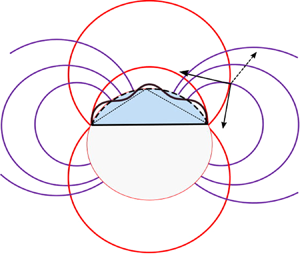
Figure 1. (a) Three-dimensional schematic of toroidal coordinate system  $\boldsymbol {r}'= \boldsymbol {r}' (\alpha , \beta , \varphi )$ overlaid on a sessile drop. Based on Li, Kar & Kumar (Reference Li, Kar and Kumar2019). (b) Diametral section of the drop (blue shaded region) with toroidal gridlines embedded into it. On a red circle, $\beta$ is constant, on a purple circle, $\alpha$ is constant. Defining expressions for $\alpha$ and $\beta$ are also displayed.
The purpose of this work is to show that our model, based on toroidal coordinates, yields fully analytical solutions for the case of an inviscid drop with fixed CL in the shape of a spherical cap. Stating the hydrodynamic equations with boundary conditions, we perform an eigenmode analysis to find the solution (§ 2). This model is then used to identify resonant frequencies for zonal, sectoral and tesseral vibration modes (§ 3). Its predictions are compared with experimental data reported in the literature. Future work and possible extensions of this model are discussed in (§ 4).
2. Theory
2.1. Sessile-drop geometry
The liquid–vapour interface of a sessile drop with contact angle  $\theta _{c} \in (0,{\rm \pi} )$ can be expressed in toroidal coordinates as $\boldsymbol {r}'= \boldsymbol {r}'(\alpha , \beta , \varphi )$ (figure 1a). Variable $\alpha \in [0,\infty )$ varies along the surface $\partial D_{f}$, where $\beta \in [0,{\rm \pi} ]$ is the angle subtended by foci $F_{1}, F_{2}$ on $\partial D_{f}$ and $\varphi \in [0,2{\rm \pi} ]$ varies in the azimuthal direction. The equilibrium (base) state $\varGamma$ of the drop can be defined as
 \begin{equation} \beta = \beta_{0}, \quad \alpha \in [0,\infty],\quad \varphi \in [0,2{\rm \pi}]. \end{equation}
A small perturbation  $\eta ' (\alpha , \varphi , t)$ on $\varGamma$ (with the CL being fixed) leads to a competition between the drop's inertia and capillarity, and the resulting motion is oscillatory in nature (cf. figure 1b). These disturbances are often expressed in terms of
 \begin{equation} h_{\alpha}' =h_{\beta}'=\frac{c}{\cosh{\alpha} - \cos{\beta}}, \quad h_{\varphi}' =\frac{c \sinh\varphi}{\cosh \alpha - \cos\beta}, \end{equation}
where  $c$ is the drop contact radius and $h_{\alpha }'$, $h_{\beta }'$ and $h_{\varphi }'$ are the scale factors of the toroidal system. Here the prime notation indicates that the variables are dimensional. In the following text, prime notation will be dropped from dimensionless variables, except for density $\rho$, surface tension $\gamma$ and contact radius $c$ of the drop. The scale factor quantifies the change in position of a point on changing one of its coordinates, so a ${\rm \Delta} \alpha$ change in $\alpha$ (keeping other coordinates constant) corresponds to a change in distance along $\hat {\alpha }$ of $h_{\alpha }'{\rm \Delta} \alpha$ (cf. figure 1a).
2.2. Equations and boundary conditions
The flow is assumed to be incompressible and irrotational. The velocity field  $\boldsymbol {v}'$ is described as $\boldsymbol {v}'= \boldsymbol {\nabla } \psi '$, where the velocity potential $\psi '$ satisfies Laplace's equation
 \begin{equation} \nabla^{2} \psi' = 0 \quad [D], \end{equation}
in the drop domain  $D$. The equation becomes closed form when subject to the no-penetration condition
 \begin{equation} \boldsymbol{\nabla} \psi' \boldsymbol{\cdot} \boldsymbol{\beta} = \frac{1}{h_{\beta}'}\frac{\partial \psi'}{\partial \beta} = 0 \quad [\partial D_{s}:= \beta = {\rm \pi}], \end{equation}
at the substrate  $\partial D^{s}$, and a free-surface kinematic boundary condition
 \begin{equation} \boldsymbol{\nabla} \psi' \boldsymbol{\cdot} \boldsymbol{\beta} = \frac{1}{h_{\beta}'}\frac{\partial \psi'}{\partial \beta}= \frac{\partial \eta'}{\partial t'} \quad [\partial D_{f} := \beta = {\rm \pi}- \theta_{c}], \end{equation}
at the interface  $\partial D_{f}$, where the normal velocity is set equal to the time derivative of perturbation. For an inviscid fluid, applying linear wave theory, the pressure field is described by the momentum equation
 \begin{equation} p' ={-} \rho \frac{\partial \psi'}{\partial t'} \quad[D]. \end{equation}
A small disturbance  $\eta '$ to the equilibrium surface $\varGamma$ causes a deviation from the initially spherical shape which is described by the modified Laplace equation
 \begin{equation} \frac{p'}{\gamma} ={-} (k_{1}^{2}+k_{2}^{2})\eta' - \varDelta_{T} \eta', \end{equation}
where  $k_{1}$, $k_{2}$ are the principal curvatures, $\varDelta _{T}$ is the Laplace–Beltrami operator; definitions are given in Appendix A. In subsequent sections, we have replaced the term $\cosh {\alpha }-\cos {\beta }$ with $b(\alpha ,\beta )$ while simplifying the terms involving scale factors $h_{\alpha }'$, $h_{\beta }'$ and $h_{\varphi }'$.
2.3. Curvatures and Laplace–Beltrami operator for toroidal coordinates
The first and second fundamental forms of a surface allow the calculation of curvature and Laplace–Beltrami operators, respectively, for a parametric surface  $\boldsymbol {x}(u^{1}, u^{2})$. The coefficients for first fundamental form are given by the metric tensor
 \begin{equation} g_{ij} \equiv \boldsymbol{x}_{i} \boldsymbol{\cdot} \boldsymbol{x}_{j} = \begin{pmatrix} E & F \\ F & G \end{pmatrix}, \end{equation}
where  $\boldsymbol {x}_{i}={\partial \boldsymbol {x}}/{\partial u^{i}}$, $\boldsymbol {x}_{j}={\partial \boldsymbol {x}}/{\partial u^{j}}$ and $i,j$ = $1, 2$ (Kreyszig Reference Kreyszig1959). The derivation of the principal curvatures and the Laplace–Beltrami operator from the coefficients $E$,
$E$,  $F$ and $G$ is given in Appendix A.
2.4. Reduction to eigenmode problem
The characteristic length scale assumed in this problem is the contact radius of the drop,  $c$. Performing a dimensional analysis on the six parameters; $p', \psi ',t',\rho ,\gamma$ and $c$ (or equivalently $\eta '$) involved in (2.6) and (2.7) gives rise to three dimensionless parameters: ${\psi ' t'}/{c^{2}}$, ${\gamma t'^{2}}/{\rho c^{3}}$ and ${p' t'^{2}}/{\rho c^{2}}$, giving characteristic scalings of $\sqrt {{\rho c^{3}}/{\gamma }}$ (time), $\sqrt {{\gamma }/{\rho c}}$ (velocity) and ${\gamma }/{c}$ (pressure).
A drop with pinned CL is subjected to a small perturbation  $\eta '(\alpha ,\varphi ,t')$. Resolving dimensional $\eta '$ and $\psi '$ into individual components (Drazin Reference Drazin2002), dimensionless eigenfunctions $y(\alpha )$ and $\phi (\beta ,\alpha )$, normal modes (frequency $\varOmega$) and azimuthal direction (wavenumber $l$), gives
 \begin{equation} \eta'(\alpha, \varphi, t') = c\,y\,(\alpha) \, \textrm{e}^{\textrm{i}\varOmega' t'} \textrm{e}^{\textrm{i}l \varphi}, \quad \psi'(\boldsymbol{r}', t') = \sqrt{\frac{\gamma c}{\rho}} \phi(\beta, \alpha) \, \textrm{e}^{\textrm{i}\varOmega' t'} \textrm{e}^{\textrm{i}l \varphi}. \end{equation}
Substituting equation (2.9a,b) into equations (2.3)–(2.7) yields
 \begin{gather} \frac{\partial}{\partial \beta} \left( h_{\varphi} \frac{\partial \phi}{\partial \beta}\right) + \frac{\partial}{\partial \alpha} \left( h_{\varphi} \frac{\partial \phi}{\partial \alpha}\right)-\frac{l^{2}}{b(\alpha,\beta)\sinh \alpha}\phi=0 \quad [D], \end{gather}
 \begin{gather}\frac{\partial \phi}{\partial \beta} = 0 \quad [\partial D_{s}:= \beta = {\rm \pi}], \end{gather}
 \begin{gather}\frac{\partial \phi}{\partial \beta} = \frac{i \lambda y}{b(\alpha,\beta_{0})} \quad [\partial D_{f} := \beta = {\rm \pi}- \theta_{c}], \end{gather}
 \begin{gather}i \lambda \phi = 2 \sin^{2}\beta y + b^{2}(\alpha,\beta_{0})\left[\frac{1}{\sinh\alpha}\frac{\partial}{\partial \alpha}\left(\sinh\alpha \frac{\partial y}{\partial \alpha}\right) - \frac{l^{2} y}{\sinh^{2} \alpha} \right], \end{gather}
 \begin{gather}\lambda^{2}= \frac{\rho \varOmega'^{2}c^{3}}{\gamma}, \end{gather}
where  $b(\alpha ,\beta _{0})$ means that it is defined on the interface $\varGamma := \beta =\beta _{0}$. Equation (2.10a) is Laplace's equation in separated form, (2.10b) is the no-penetration boundary condition, (2.10c) and (2.10d) are free-surface kinematic boundary conditions, and (2.10e) gives the dimensionless frequency $\lambda$. It should be noted that all variables in (2.10a)–(2.10d) are dimensionless, hence without prime notation.
2.5. Solving the eigenmode equations
The solution to (2.10a) in the toroidal system is given by Lebedev (Reference Lebedev1965) as
 \begin{equation} \phi = a [A P_{v-{1}/{2}}^{l}(\cosh\alpha)+ B Q_{v-{1}/{2}}^{l} (\cosh\alpha)] [ C \cos{v\beta} +D \sin{v\beta} ], \end{equation}
where  $a=\sqrt {2(\cosh \alpha -\cos \beta )}$, $P_{v-{1}/{2}}^{l}(\cosh \alpha )$ and $Q_{v-{1}/{2}}^{l}(\cosh \alpha )$ are Legendre functions of the first and second kind (also called toroidal functions), with $v$ the toroidal degree and $l$ the azimuthal order. At $\alpha =0$, $P_{v}^{l}(1)=1$ and $\lim _{z\to 1+}$ $Q_{v}^{l}(z)=\infty$, which means that the latter is not defined at the apex of the drop. Thus, setting $B=0$ and $v=i\tau$ (see Lebedev Reference Lebedev1965, p. 227) gives
 \begin{equation} \phi = a P_{i\tau-{1}/{2}}^{l}(\cosh\alpha) [C \cos i\tau\beta + D \sin i\tau\beta]. \end{equation}
Using (2.10) and substituting  $\beta ={\rm \pi}$ in (2.10b) gives $C = - iD \coth {\rm \pi}$. Upon further simplification (2.12) reduces to
 \begin{equation} \phi = a P(\cosh\alpha) f(\tau\beta), \end{equation}
where  $P(\cosh {\alpha })$ denotes $P_{i\tau - 1/2}^{l}(\cosh {\alpha })$ and $f(\tau \beta )=\sinh \tau \beta -\coth \tau {\rm \pi}\cosh \tau \beta$. Substituting (2.13) into (2.10c) (after multiplying both sides by $b(\alpha ,\beta _{0})$) gives
 \begin{equation} i\lambda y = b(\alpha,\beta_{0}) \frac{\partial \phi}{\partial \beta}= P b(\alpha,\beta_{0}) \left(\frac{f}{a} \sin\beta_{0} + \tau a \,f_{1}\right) = P T, \end{equation}
where  $T(\alpha ,\beta _{0})= b(\alpha ,\beta _{0}) (({f}/{a}) \sin \beta _{0} + \tau a \,f_{1})$ and $f_{1}=\cosh \tau \beta _{0}-\coth \tau {\rm \pi}\sinh \tau \beta _{0}$. Functions $T(\alpha ,\beta _{0})$, $f(\tau \beta _{0})$, $f_{1}(\tau \beta _{0})$ and $P(\cosh \alpha )$ are written without arguments for clarity.
An important consequence of (2.14) is that  $y=0$ at the CL, which arises because $P\rightarrow 0$ as $\alpha \rightarrow \infty$, and so use of the toroidal coordinate system imposes the fixed CL condition on the problem. The mobility of the CL is defined as $1/\varLambda$ by $Bo$–
$Bo$– $St$, which is zero for an immobile CL and infinite for a fully mobile CL. Only the immobile CL case, $\varLambda = 0$, is considered in the current work.
Substituting the above equation into (2.10d) gives, at  $\beta =\beta _{0}$,
 \begin{equation} -\lambda^{2}\phi = 2\sin^{2}\beta_{0}PT + b^{2}(\alpha,\beta_{0})\left[\frac{1}{\sinh\alpha}\frac{\partial}{\partial \alpha} \left(\sinh\alpha \frac{\partial}{\partial \alpha}(PT) \right) - \frac{l^{2}}{\sinh^{2} \alpha} PT \right]. \end{equation}
This can be rearranged as
 \begin{equation} -\lambda^{2} \phi = 2 \sin^{2}\beta_{0} PT + b^{2}(\alpha,\beta_{0})[I T + II], \end{equation}
where  $I$ and $II$ are, respectively,
 \begin{gather} I = \frac{1}{\sinh\alpha}\frac{\partial}{\partial \alpha} \left(\sinh\alpha \frac{\partial P}{\partial \alpha} \right) - \frac{l^{2}}{\sinh^{2}\alpha} P, \end{gather}
 \begin{gather}II = \frac{\partial T}{\partial \alpha}\frac{\partial P}{\partial \alpha}+ \frac{1}{\sinh\alpha}\frac{\partial}{\partial\alpha}\left(\sinh\alpha P \frac{\partial T}{\partial \alpha} \right). \end{gather}
The term  $I$ is equivalent to $(v^{2}-\frac {1}{4})P$ (see Lebedev Reference Lebedev1965, p. 224). In fact, an analogous simplification is performed while deriving an expression for the eigenfrequencies of a free spherical drop in Rayleigh's derivation (see Landau & Lifshitz Reference Landau and Lifshitz1987, p. 246). Further simplification of the right-hand side of (2.16) gives
 \begin{align} -\lambda^{2}\!=\! \left[2\sin^{2}\beta_{0}\!-\!b^{2}(\alpha,\beta_{0})\left( \tau^{2}\!+\!\frac{1}{4} \right) \right]\frac{T}{af} + \frac{b^{2}(\alpha,\beta_{0})}{af}\left[T_{\alpha}\left(\frac{2 P_{\alpha}}{P}+\coth\alpha\right)+T_{\alpha \alpha} \right], \end{align}
where a single or double subscript  $\alpha$ on a function denotes single or double derivative of the function with respect to $\alpha$. The expressions for $T_{\alpha }, T_{\alpha \alpha }, P$ and $P_{\alpha }$ (which fall under the class of hypergeometric functions) are given in Appendix B.
3. Results
The variation of dimensionless frequency  $\lambda$ with contact angle $\theta _c = {\rm \pi}-\beta _0$ is determined by solving (2.18). Previous studies such as $Bo$–
$Bo$– $St$ classified the vibrational modes as zonal ( $l=0$), sectoral ( $\tau =l$) and tesseral ( $l\neq 0, \tau \neq l$). Results are presented for each type of mode in turn.
3.1. Zonal ( $l=0$) modes

When the disturbance of the interface is axisymmetric, the mode shapes are termed zonal. For a sessile drop of fixed contact radius  $c$, increasing the contact angle $\theta _{c}$ increases the volume of the drop (inertia) and thus decreases the frequency $\lambda$ (cf. figure 2a). There is excellent agreement between the model and the data of Chang et al. (Reference Chang, Bostwick, Daniel and Steen2015) in this figure, particularly at higher mode numbers. For instance, for $\tau =10$ and $\theta _{c}=40^{\circ }$, our model overpredicts slightly, by a factor of 1.05, while the $Bo$–
$Bo$– $St$ model overpredicts by a factor of 1.25 (see the inset to figure 2a). For the other modes at $\theta _{c}<60^{\circ }$, the agreement is better than the $Bo$–
$Bo$– $St$ model. Higher mode numbers correspond to more points (nodes) of intersection of the disturbed interface $\delta D_{f}$ with the undisturbed interface $\varGamma$. As there is no variation in the azimuthal direction, a front view (see the inset to figure 2b) is sufficient to describe the mode shape. This figure shows the case with 10 nodes ( $\tau =10$).

Figure 2. Results for zonal modes,  $m=0$. (a) Effect of contact angle $\theta _{c}$ on dimensionless frequency $\lambda$ for toroidal mode number $\tau$. Solid lines are solutions to (2.18) and symbols are the experimental values reported by Chang et al. (Reference Chang, Bostwick, Daniel and Steen2015). Inset shows the comparison of same experiments with $Bo$–
$Bo$– $St$ model (dashed lines). Effect of $\tau$ on $\lambda$ (b) and $\varOmega '$ (c). Symbols show experimental values reported by (b) Chang et al. (Reference Chang, Bostwick, Steen and Daniel2013) and (c) Mettu & Chaudhury (Reference Mettu and Chaudhury2012) for a water drop. Loci show model predictions for different contact angles: (b) solid line, $\theta _{c}=68.6^{\circ }$; dashes, $\theta _{c}=63.6^{\circ }$; dots, $\theta _{c}=73.6^{\circ }$; (c) solid line, $\theta _{c}=79.5^{\circ }$; dashes, $\theta _{c}=68^{\circ }$; dots, $\theta _{c}=91^{\circ }$. Inset in (b) shows interface shape $y$ plotted on $\varGamma$ using (2.18) for $\tau =10$ (not to scale).
Further comparisons of predicted zonal mode frequencies with experimental measurements are shown for the data sets reported by Chang et al. (Reference Chang, Bostwick, Steen and Daniel2013) and Mettu & Chaudhury (Reference Mettu and Chaudhury2012) in figures 2(b) and 2(c), respectively. In the former, the experimental values lie within the range of theoretical frequencies calculated for the range of contact angles  $\theta _{c}$ involved. For the higher modes, $\tau = 8$ and 10, the frequencies lie at the upper end of the theoretical span, where there were a limited number of data points as these require larger droplets ( ${\gtrsim}5{\rm \mu} {\rm L}$ (see Mettu & Chaudhury Reference Mettu and Chaudhury2012, figure 4a), whereas lower modes ( $\tau =2,4,6$) were experimentally accessible for droplets with smaller volume, ${\leq}5{\rm \mu} {\rm L}$. In addition, there is a small increase in slope for $\tau =10$ (compared to slope at $\tau =6$); this feature is also present in figure 2(a) for $\theta _{c}\approx 65^{\circ }$. In figure 2(c), the width of the predicted frequency band is small and lies at the lower end of the range of observed frequencies. A possible explanation for this mismatch is that the model neglects contributions from viscous effects. Chang et al. (Reference Chang, Bostwick, Steen and Daniel2013) reported that the bandwidth of predicted frequencies increased when viscous contributions were added (noting that the dimensional frequency is plotted here). Chang et al. (Reference Chang, Bostwick, Daniel and Steen2015) subsequently showed that the viscous contribution is characterised by the Ohnesorge number, $Oh=\mu /\sqrt {\rho c \gamma }$, and even at a small value of $Oh=0.003$ for water (instead of $Oh=0$ for the inviscid case) the resonant peak changed from an infinite to a finite value and, thus, increased the bandwidth of predicted frequency (see Chang et al. Reference Chang, Bostwick, Daniel and Steen2015, p. 446). The effect of viscosity on a drop undergoing oscillations of arbitrary amplitude has been discussed both for free drops and sessile/pendant drops (see Basaran Reference Basaran1992 and Wilkes & Basaran Reference Wilkes and Basaran1997). For the latter case, it has been reported that as the viscosity increases, the resonant frequency also increases, so that excluding viscous effects can lead to predicted frequencies lying at the lower end of the observed spectrum.
3.2. Sectoral ($\tau =l, l\neq 0$) modes

A non-axisymmetric mode with wavenumber pair  $[\tau ,l]$ has $l$ longitudinal intersections and $(\tau -l)/2$ latitudinal intersections (or $\tau -l$ nodes on the interface) with the undisturbed interface $\varGamma$ (see Bostwick & Steen Reference Bostwick and Steen2014, p. 19). A sectoral mode, with $\tau =l$, is a special case where there are only longitudinal intersections. Figure 3 compares the experimental frequencies reported by Chang et al. (Reference Chang, Bostwick, Daniel and Steen2015) with our model and the $Bo$–
$Bo$– $St$ model. There is good agreement with our model for $\tau =9$. For $\tau = 5$ and 7, the two models bracket the data.

Figure 3. Effect of contact angle on dimensionless frequency for sectoral modes,  $\tau =l$, for (a) $[5,5]$, (b) $[7,7]$ and (c) $[9,9]$. Solid loci show the solutions to (2.18), dashed loci are the results presented by Bostwick & Steen (Reference Bostwick and Steen2014). Symbols indicate experimental data reported by Chang et al. (Reference Chang, Bostwick, Daniel and Steen2015).
3.3. Tesseral ($\tau \neq l,\ l\neq 0$) modes

A tesseral mode shape with wavenumber pair  $[\tau ,l]$ has non-zero longitudinal and latitudinal intersections because $\tau \neq l$. Figure 4 compares the results for our model and the $Bo$–
$Bo$– $St$ model in a similar fashion to the sectoral mode. For the $\tau =9$ cases, our model agrees with the experimental data quite well for all $\theta _{c}$ values investigated. For $\theta _{c} \leq 65^{\circ }$, the $Bo$–
$Bo$– $St$ model does not capture the observed trend, for $50^{\circ }$ and $l=7$, it overpredicts by a factor of 1.17, whereas our model underpredicts slightly by a factor of 1.05. For $\tau =7$, there is good agreement between the experimental data and both models as $\theta _{c}$ decreases from $140^{\circ }$ to $70^{\circ }$, below which our model continues to perform well and $Bo$–
$Bo$– $St$ starts to diverge. For $\tau =5$, our model captures the frequencies at low $\theta _{c}$ whereas the $Bo$–
$Bo$– $St$ model works well at higher values.

Figure 4. Effect of contact angle on dimensionless frequencies for tesseral modes with  $[\tau ,m]$ values of (a) $[5,3]$, (b) $[7,5]$, (c) $[9,5]$ and (d) $[9,7]$. Solid loci show the solutions to (2.18)), dashed lines are the results presented by Bostwick & Steen (Reference Bostwick and Steen2014). Symbols show experimental data reported by Chang et al. (Reference Chang, Bostwick, Daniel and Steen2015). The shaded region in (d) represents the range of frequencies calculated using VPF theory by Chang et al. (Reference Chang, Bostwick, Daniel and Steen2015) for water, with substrate forcing and viscosity included.
It should be noted that our model cannot predict the frequencies for small contact angles, because in this case a larger fraction of the sessile-drop volume lies within the solid–liquid boundary layer and drop–substrate interactions then cause damping of oscillations. The range of contact angles suggested to avoid boundary layer viscous dissipation effects, discussed in Sharp (Reference Sharp2012), is  $30^{\circ }\text {--}150^{\circ }$.
For the lowest mode,  $[5,3]$, there is a slight overprediction for larger contact angles. This can be attributed to the assumption of a pinned CL in the current work. If the CL is, instead, assumed to be mobile and not pinned, the slope of the frequency-versus-contact-angle curve will decrease at larger contact angles (see Bostwick & Steen Reference Bostwick and Steen2014, figures 10 and 11). This represents a limitation in the current model in that mobile CL behaviour is not readily incorporated in the toroidal coordinate approach.
4. Discussion and conclusions
The superior performance of our model for lower  $\theta _{c}$ and higher modes is probably the result of using toroidal coordinates, which fit the sessile drop naturally. An interesting physical insight from this work is that the slope of the $\lambda$ versus $\theta _{c}$ curve decreases as $\theta _{c}$ decreases; the curve almost reaching a plateau. This is also suggested by experiments. The physical models present in literature incorporate bulk dissipation and CL (Davis) dissipation, e.g. Bostwick & Steen (Reference Bostwick and Steen2016), to account for this plateau. On the one hand, the current toroidal model, while established on zero viscosity and fixed CL assumptions, can still predict this plateau with good success. On the other hand, incorporating more dissipation terms will improve this model and bring more understanding of observations such as mode mixing and mode competition (Bostwick & Steen Reference Bostwick and Steen2015). Note that the strength of this inviscid theory coupled with an appropriate coordinate system points to the importance of choosing a framework which maps the complicated geometries of physics problems perfectly, as previously done in Fokas & Nachbin (Reference Fokas and Nachbin2012) and Richardson (Reference Richardson1992).
There are exceptions, e.g. figures 3(a) and 4(a), and we here consider whether the mismatch between the predictions of the model and the experimental data could arise from the assumptions made in our model. The larger error incurred by the  $Bo$–
$Bo$– $St$ model can be attributed to the approach used to enforce the no-penetration condition. Earlier works on constrained drops (e.g. Ramalingam, Ramkrishna & Basaran Reference Ramalingam, Ramkrishna and Basaran2012 and Prosperetti Reference Prosperetti2012) essentially used the Lagrange multiplier method to enforce the no-penetration condition at the pinning circle and these methods permitted a discontinuity in the interface shape at the contact point. The $Bo$–
$Bo$– $St$ method does not allow a discontinuity at the pinning sites, which leads to overprediction of the frequency (see Bostwick & Steen Reference Bostwick and Steen2015, p. 558).
The model considers the sessile drop on a substrate as a mass–spring system, where viscous effects and substrate–drop interactions are neglected. These assumptions were also made in the  $Bo$–
$Bo$– $St$ model and were subsequently relaxed in their subsequent work, for example, Bostwick & Steen (Reference Bostwick and Steen2016), where they studied damping for viscous drops (with fixed CL) undergoing substrate-forced oscillation. To extend our model along the lines discussed in Chang et al. (Reference Chang, Bostwick, Daniel and Steen2015), viscous contributions could be incorporated by adding a damping term, $i \lambda \epsilon C[y]$, to the right-hand side of (2.15), where $C$ is the dissipation operator and $\epsilon ={\mu }/{(\rho c \gamma )^{1/2}}$ is the Ohnesorge number. Substrate–drop interactions can be modelled using two main assumptions: (i) constant contact radius; and (ii) modelling the substrate forcing via the bulk pressure in the drop in the form of Faraday oscillations. With regard to (i), it should be noted that contact-angle hysteresis on the modes cannot be incorporated using the toroidal framework presented here because it requires the incorporation of a dynamic CL condition (Bostwick & Steen Reference Bostwick and Steen2014). With (ii), the substrate contribution is incorporated by adding a term $F_{0}\textrm {e}^{\textrm {i}\lambda t}$ to the right-hand side of (2.15), where $\lambda$ is the frequency of substrate forcing (not the natural frequency) and $F_{0}$ its amplitude. Chang et al. (Reference Chang, Bostwick, Daniel and Steen2015) used these assumptions and incorporated the aforementioned effects in their viscous potential flow (VPF) theory. The envelope of solutions which they obtained is shown as a shaded region in figure 4(d) and it spans $Bo$–
$Bo$– $St$ and our model (both inviscid). It is, thus, expected that the addition of viscous and substrate contributions to our model will modify (2.18) and increase the bandwidth of predicted frequencies. This is the subject of ongoing work, where the aim is to identify the contributions of viscous damping and substrate forcing, and thereby establish when significant differences will arise from the inviscid model.
The description of an oscillating drop presented here is not suitable for cases where the drop shape is influenced by gravity, which is quantified by  $Bo$ (ratio of gravity to surface tension). As the volume of the drop increases, the drop shape changes from that of a truncated sphere ( $Bo=0$), towards being ellipsoidal ( $0< Bo<5$) until it forms a flat puddle ( $Bo>5$), with uniform depth except near the edges (Lubarda & Talke Reference Lubarda and Talke2011). We believe that it should be possible to model a flattened drop using confocal ellipsoidal coordinates system in the $0.5< Bo<5$ regime. Finding resonant frequencies for a flattened drop will allow us to extend our $Bo=0$ theory to $0< Bo<5$, and compare the results with the theory for flattened drops presented by Noblin, Buguin & Brochard-Wyart (Reference Noblin, Buguin and Brochard-Wyart2004) where the drop is modelled as a liquid bath and the resonant frequency is that associated with a standing wave on its interface.
This work introduces, for the first time, an analytical solution to the sessile-drop oscillation problem. The superiority of this model lies in the fact that its predictions work well for lower contact angles ( ${<}75^{\circ }$) compared with the existing models. It also predicts a decrease in slope as $\theta _{c}$ decreases, which is consistent with experiments. The behaviour at lower contact angles ( ${<}30^{\circ }$) remains to be experimentally validated (and physically understood) for all types of modes.
To summarise, our model provides a concise solution to the sessile-drop oscillation problem which opens a new window to researchers interested in this and related problems. A clear next step could be to test the  $\theta _{c}<30^{\circ }$ regime experimentally, model a drop being vibrated on an inclined plane (see Brunet, Eggers & Deegan Reference Brunet, Eggers and Deegan2007) and extend the model to larger drops by including the effects of gravity.
Acknowledgements
We wish to thank Dr R.K. Bhagat for fruitful discussions on this problem. S.S. also benefitted greatly from insights provided by Dr H. Tankasala and A.J.D. Shaikeea. We would like to thank an anonymous reviewer for greatly helping in improving the mathematical presentation of this work.
Funding
S.S. was funded by the Cambridge India Ramanujan Scholarship from the Cambridge Commonwealth, European and International Trust and SERB, Govt. of India.
Declaration of interests
The authors report no conflict of interest.
Appendix A. Differential geometry of the toroidal system
A general point on the surface  $\beta =\beta _{0}$ is $\boldsymbol {x}(\alpha ,\varphi )= (x,y,z)$ such that
 \begin{equation} x = \frac{c \sinh\alpha \cos\varphi}{b}, \quad y = \frac{c \sinh\alpha \sin\varphi}{b}, \quad z = \frac{c \sin\beta}{b}, \end{equation}
where  $b \equiv b(\alpha ,\beta ) = \cosh \alpha - \cos \beta$ (see Lebedev Reference Lebedev1965, p. 222). Putting $i=\alpha$, $j=\varphi$ in (2.8) gives
 \begin{equation} \left.\begin{array}{c} \displaystyle \boldsymbol{x}_{\alpha} = \left(\dfrac{c \cos\varphi d }{b^{2}}, \dfrac{c \sin\varphi d }{b^{2}}, -\dfrac{c \sin\beta \sinh\alpha}{b^{2}}\right)\\ \displaystyle \boldsymbol{x}_{\varphi}= \left(\dfrac{-c \sinh\alpha \sin\varphi}{b}, \dfrac{c \sinh\alpha \cos \varphi }{b}, 0 \right)\\ \displaystyle E = \boldsymbol{x}_{\alpha} \boldsymbol{\cdot} \boldsymbol{x}_{\alpha} = \left(\dfrac{c}{b}\right)^{2}\\ F = \boldsymbol{x}_{\alpha} \boldsymbol{\cdot} \boldsymbol{x}_{\varphi} = 0 \\ \displaystyle G = \boldsymbol{x}_{\varphi} \boldsymbol{\cdot} \boldsymbol{x}_{\varphi} =\left(\dfrac{c \sinh\alpha}{b}\right)^{2}\\ \displaystyle W = \sqrt{EG-F^{2}}= \dfrac{c^{2} \sinh\alpha}{b^{2}} \end{array}\right\}, \end{equation}
where  $d = 1-\cosh \alpha \cos \beta$ and $W$ is the determinant of the metric tensor.
The coefficients of second fundamental form of surface are  $L=\boldsymbol {x}_{ii} \boldsymbol {\cdot } \boldsymbol {n}$, $M=\boldsymbol {x}_{ij} \boldsymbol {\cdot } \boldsymbol {n}$, $N=\boldsymbol {x}_{jj} \boldsymbol {\cdot } \boldsymbol {n}$ where $\boldsymbol {n}={\boldsymbol {x}_{i} \times \boldsymbol {x}_{j}}/{|\boldsymbol {x}_{i} \times \boldsymbol {x}_{j}|}$ and $|\boldsymbol {x}_{i} \times \boldsymbol {x}_{j}| = W$. Again, setting $i=\alpha$, $j=\varphi$ gives
 \begin{equation} \left.\begin{array}{c} \displaystyle L = \dfrac{ (\boldsymbol{x}_{\alpha \alpha} \boldsymbol{x}_{\alpha} \boldsymbol{x}_{\varphi})}{W} = \dfrac{-c \sin \beta }{b^{2}} \\ \displaystyle M = \dfrac{ (\boldsymbol{x}_{\alpha \varphi} \boldsymbol{x}_{\alpha} \boldsymbol{x}_{\varphi})}{W} =0 \\ \displaystyle N = \dfrac{ (\boldsymbol{x}_{\varphi \varphi} \boldsymbol{x}_{\alpha} \boldsymbol{x}_{\varphi})}{W} = \dfrac{-c \sin \beta \sinh^{2} \alpha}{b^{2}} \end{array}\right\}, \end{equation}
where the notation  $(\boldsymbol {a} \, \boldsymbol {b} \, \boldsymbol {c})$, used in Kreyszig (Reference Kreyszig1959), stands for the triple product $\boldsymbol {a} \boldsymbol {\cdot } (\boldsymbol {b}\times \boldsymbol {c})$ of vectors $\boldsymbol {a}$, $\boldsymbol {b}$ and $\boldsymbol {c}$. In (2.7), the first term in the right-hand side is then
 \begin{equation} k^{2}_{1}+k^{2}_{2}= \left(\frac{EN-2FM+GL}{W^{2}} \right)^{2} - 2 \frac{LN-M^{2}}{W^{2}} = \frac{2 \sin^{2}\beta}{c^{2}}, \end{equation}
and the second term (the Laplace–Beltrami operator) becomes
 \begin{align} \varDelta_{T}\eta & = \frac{1}{W} \left[ \frac{\partial}{\partial \alpha} \left(\frac{G\eta_{\alpha}-F\eta_{\varphi}}{W} \right) + \frac{\partial}{\partial \varphi} \left(\frac{E\eta_{\varphi}-F\eta_{\alpha}}{W} \right) \right] \nonumber\\ & = \frac{b^{2}}{c^{2}} \left[ \frac{1}{\sinh\alpha} \frac{\partial}{\partial \alpha} \left( \sinh\alpha \frac{\partial \eta}{\partial \alpha} \right) + \frac{1}{\sinh^{2}\alpha} \frac{\partial}{\partial \varphi}\left(\frac{\partial \eta}{\partial \varphi}\right)\right]. \end{align}
Another form of (A5) is derived in the notes of Deserno (Reference Deserno2004, p. 24).
Appendix B. Hypergeometric functions
Hypergeometric functions are solutions to the second-order ODE encountered while using a system of orthogonal curvilinear coordinates to solve Laplace's equation (see Lebedev Reference Lebedev1965, pp. 161–173). In our case, we use the toroidal system to solve Laplace's equation and find Legendre functions of the first kind  $P_{v}(z)$ as the solution (hence, referred to as the toroidal functions). The integral representations of these functions are given below, for different cases:
(i) When
$l=0$ (see Lebedev Reference Lebedev1965, p. 173)
(B1)for\begin{equation} P_{v}(\cosh \alpha)= A_{1} \int_{0}^{\infty} \frac{\cosh (v + {1}/{2})\theta}{\sqrt{2 \cosh \theta + 2 \cosh \alpha}} \, {\textrm{d}} \theta, \end{equation}$\alpha > 0, -1< Re(v) < 0$ and
(B2)for\begin{equation} P_{\alpha}= \frac{{\textrm{d}}}{{\textrm{d}} \alpha}(P_{v}(\cosh \alpha))= A_{1} \sinh{\alpha} \int_{0}^{\infty} \frac{-\cosh (v + {1}/{2})\theta}{(2 \cosh \theta + 2 \cosh \alpha)^{3/2}} \, {\textrm{d}} \theta, \end{equation}$\alpha > 0, -1< Re(v) < 0$. $A_{1} =({2}/{{\rm \pi} }) \cos (v + \frac {1}{2}){\rm \pi}$.(ii) When
$l\neq 0$ (see Lebedev Reference Lebedev1965, pp. 172, 199)
(B3)where\begin{equation} P_{v}^{l}(\cosh \alpha)= A_{2} \int_{-\alpha}^{\alpha} \frac{\textrm{e}^{-(v+{1}/{2})\theta} T_{l}(\cos \psi)}{\sqrt{2 \cosh \alpha - 2 \cosh \theta}} \, {\textrm{d}} \theta, \end{equation}$A_{2}={\varGamma (v+m+1)}/{{\rm \pi} \varGamma (v+1)}$, $\varGamma$ is the gamma function and $T_{l}$ is the Chebyshev polynomial.


Other functions used in (2.18) in the main text are
 \begin{equation} \frac{T_{\alpha}}{a f} = \sinh{\alpha} \left(2 \sin \beta_{0} \frac{a_{1}}{a} + \tau \frac{f_{1}}{f}\right) +b \left(2 \sinh\alpha \left(\sin\beta_{0} \frac{a_{2}}{a} + \tau \frac{f_{1}}{f} \frac{a_{1}}{a} \right) \right), \end{equation}
 \begin{align} \frac{T_{\alpha \alpha}}{a f} &= 2 \sin^{2}h \alpha \left(2 \sin \beta_{0} \frac{a_{1}}{a}+\tau \frac{f_{1}}{f} \right) + 2 \sin^{2}h\alpha \left(2 \sin\beta_{0} \frac{a_{2}}{a} + \tau \frac{f_{1}}{f} \frac{a_{1}}{a}\right) \nonumber\\ &\quad + 4b \sinh^{2} \alpha \left(2 \sin\beta_{0}\frac{a_{3}}{a}+\tau \frac{f_{1}}{f}\frac{a_{2}}{a}\right) + \cosh{\alpha} \left(2 \sin \beta_{0} \frac{a_{1}}{a}+\tau \frac{f_{1}}{f} \right) \nonumber\\ &\quad + 2b \cosh\alpha \left(2 \sin\beta_{0}\frac{a_{2}}{a}+\tau \frac{f_{1}}{f}\frac{a_{1}}{a}\right), \end{align}
where we have used the notation  $a_{1}=0.5/a$, $a_{2}=-0.25/a^{3}$, $a_{3}=0.375/a^{5}$ and $f_{1}=\cosh \tau \beta _{0}-\coth \tau {\rm \pi}\sinh \tau \beta _{0}$.


 Open access