


1 Introduction
In its simplest, one-dimensional (1-D) idealized form, a free-running, high-explosive (HE) detonation is a shock supported by the release of energy, initiated by the passage of the detonation’s shock over fresh explosive. The structure of the flow in the energy-release zone was first described by Zel’dovich, von Neumann and Döring (ZND) (Fickett & Davis Reference Fickett and Davis1979, pp. 42–51), When measured in a reference frame attached to the shock, the flow at the point where the shock crosses a particle of fresh explosive, referred to as the von Neumann (N) point, is subsonic and becomes choked or sonic at the point where the reaction in that particle is completed, referred to as the Chapman–Jouguet (CJ) point. The pressure decreases from the shock to the sonic point, as it does for flow through a gas-dynamic nozzle. Such a detonation is self-supporting and travels at the minimum allowed speed, $D_{CJ}$
.
$D_{CJ}$
.
This idealized picture must be modified when such a 1-D, ZND detonation encounters the boundaries of the explosive. Depending on the angle of incidence, $\unicode[STIX]{x1D714}$
, of the detonation with the HE’s boundary (see figure 1) and the properties of the inert material against the HE providing confinement to the detonation, a number of different situations can arise (Aslam, Bdzil & Stewart Reference Aslam, Bdzil and Stewart1996; Bdzil & Stewart Reference Bdzil, Stewart and Zhang2012; Short & Quirk Reference Short and Quirk2018).
$\unicode[STIX]{x1D714}$
, of the detonation with the HE’s boundary (see figure 1) and the properties of the inert material against the HE providing confinement to the detonation, a number of different situations can arise (Aslam, Bdzil & Stewart Reference Aslam, Bdzil and Stewart1996; Bdzil & Stewart Reference Bdzil, Stewart and Zhang2012; Short & Quirk Reference Short and Quirk2018).
Here, we focus on detonations for which $\unicode[STIX]{x1D714}=90^{\circ }$
initially; i.e. detonations whose basic direction of propagation is parallel to the undisturbed interface between the fresh explosive and the inert material serving as confinement for the HE. Since the detonation pressures of high explosives are of the order of 200 000 atmospheres (20 GPa), which is greater that the strength of all materials, the confinement yields and is deflected by the passage of the detonation. As the confinement deflects in response to the pressure in the explosive’s reaction zone, a steep rarefaction is able to propagate into the explosive’s reaction zone, since the flow in the reaction zone and near the detonation shock is initially subsonic in the detonation shock-attached reference frame. With time, the rarefaction propagates deep into the subsonic detonation reaction zone, which leads to far-reaching changes to the reaction zone, eventually leading to the establishment of a fully multidimensional, steady-state detonation (see figure 1). Given that the detonation speed exceeds
$\unicode[STIX]{x1D714}=90^{\circ }$
initially; i.e. detonations whose basic direction of propagation is parallel to the undisturbed interface between the fresh explosive and the inert material serving as confinement for the HE. Since the detonation pressures of high explosives are of the order of 200 000 atmospheres (20 GPa), which is greater that the strength of all materials, the confinement yields and is deflected by the passage of the detonation. As the confinement deflects in response to the pressure in the explosive’s reaction zone, a steep rarefaction is able to propagate into the explosive’s reaction zone, since the flow in the reaction zone and near the detonation shock is initially subsonic in the detonation shock-attached reference frame. With time, the rarefaction propagates deep into the subsonic detonation reaction zone, which leads to far-reaching changes to the reaction zone, eventually leading to the establishment of a fully multidimensional, steady-state detonation (see figure 1). Given that the detonation speed exceeds $6000~\text{m}~\text{s}^{-1}$
, being greater than the acoustic speed in the confiner material, a narrow layer of supersonic flow, pulled along by the detonation, is induced into the confinement material.
$6000~\text{m}~\text{s}^{-1}$
, being greater than the acoustic speed in the confiner material, a narrow layer of supersonic flow, pulled along by the detonation, is induced into the confinement material.

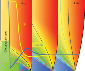
Figure 1. The long-time, steady-state detonations that develop when an 1-D, ZND detonation, with an initial angle of incidence with the confiner interface of $\unicode[STIX]{x1D714}=90^{\circ }$
, adjusts to the rarefactions generated as the detonation deflects the confiner interface. (a,b) Display the cases for a high-impedance and low-impedance inert material, respectively. A smooth flow is observed for the high-impedance (confined) case, while a rarefaction fan is observed at the edge for the low-impedance (unconfined) case (Bdzil & Stewart Reference Bdzil, Stewart and Zhang2012).
$\unicode[STIX]{x1D714}=90^{\circ }$
, adjusts to the rarefactions generated as the detonation deflects the confiner interface. (a,b) Display the cases for a high-impedance and low-impedance inert material, respectively. A smooth flow is observed for the high-impedance (confined) case, while a rarefaction fan is observed at the edge for the low-impedance (unconfined) case (Bdzil & Stewart Reference Bdzil, Stewart and Zhang2012).
As displayed in figure 1, the steady-state form that the detonation eventually takes depends on the strength (shock impedance) of the confiner. A more rigid, higher-impedance confiner leads to the two-dimensional (2-D) detonation shown in figure 1(a), while a weaker, lower-impedance confiner leads to a detonation that propagates as if it were a fully unconfined detonation, as shown in figure 1(b) (Bdzil & Stewart Reference Bdzil, Stewart and Zhang2012). The confined detonation, shown in figure 1(a), more nearly resembles a weakly perturbed 1-D detonation, with the HE /confiner interface showing a relatively small deflection, and the related shock-edge angle, $\unicode[STIX]{x1D714}$
, being only slightly smaller than the original 1-D value,
$\unicode[STIX]{x1D714}$
, being only slightly smaller than the original 1-D value, $\unicode[STIX]{x1D714}=90^{\circ }$
. When measured in the reference frame moving along the undisturbed confiner interface with the intersection point of the detonation shock and that interface, the flow immediately behind the detonation shock is subsonic, as in a 1-D detonation. The speed of the intersection point, referred to as the detonation phase velocity,
$\unicode[STIX]{x1D714}=90^{\circ }$
. When measured in the reference frame moving along the undisturbed confiner interface with the intersection point of the detonation shock and that interface, the flow immediately behind the detonation shock is subsonic, as in a 1-D detonation. The speed of the intersection point, referred to as the detonation phase velocity, $D_{0}$
, is given as
$D_{0}$
, is given as
 $$\begin{eqnarray}D_{0}=D_{ne}/\sin (\unicode[STIX]{x1D714}_{e}),\end{eqnarray}$$
where $\unicode[STIX]{x1D714}_{e}$
and
$\unicode[STIX]{x1D714}_{e}$
and $D_{ne}<D_{CJ}$
are the shock angle and detonation velocity normal to the shock at the HE edge. The detonation shock pressure at the edge,
$D_{ne}<D_{CJ}$
are the shock angle and detonation velocity normal to the shock at the HE edge. The detonation shock pressure at the edge, $P_{e}$
, is
$P_{e}$
, is $P_{e}=O(\unicode[STIX]{x1D70C}_{0}D_{ne}^{2})$
, which is less than that of the 1-D detonation shock pressure, and where
$P_{e}=O(\unicode[STIX]{x1D70C}_{0}D_{ne}^{2})$
, which is less than that of the 1-D detonation shock pressure, and where $\unicode[STIX]{x1D70C}_{0}$
is the density of the un-shocked, fresh explosive.
$\unicode[STIX]{x1D70C}_{0}$
is the density of the un-shocked, fresh explosive.
The 2-D partial-differential equations (PDEs) that govern the flow in the subsonic region of the reaction zone are of elliptic type (Carrier & Pearson Reference Carrier and Pearson1976), and admit only smooth solutions. This mathematics then argues for the absence of reflected waves, such as shocks and rarefaction fans in multidimensional subsonic flows, such as those of the detonation reaction zone. Instead, the detonation adjusts the shape of the lead shock such that a reflected wave is not needed to turn the flow once a steady state is established.
For the unconfined detonation displayed in figure 1(b), the HE /confiner interface shows a much larger deflection, due to the weakness of the confiner and the ease with which the confiner can be deformed. The shock angle at the edge, $\unicode[STIX]{x1D714}_{s}$
, is now seen to be considerably smaller than
$\unicode[STIX]{x1D714}_{s}$
, is now seen to be considerably smaller than $\unicode[STIX]{x1D714}=90^{\circ }$
. If we assume that
$\unicode[STIX]{x1D714}=90^{\circ }$
. If we assume that $D_{0}$
is the same here as in figure 1(a), which is the case if both explosive charges are very wide, then
$D_{0}$
is the same here as in figure 1(a), which is the case if both explosive charges are very wide, then $D_{ne}$
would be considerably below the value it would have for the highly confined detonation of figure 1(a). Then the pressure, which goes as
$D_{ne}$
would be considerably below the value it would have for the highly confined detonation of figure 1(a). Then the pressure, which goes as $O(\unicode[STIX]{x1D70C}_{0}D_{ne}^{2})$
, would be much reduced compared with that for the figure 1(a) case. This drop in pressure brings with it a drop in the sound speed near the shock, and the sonic locus, which is far back in the flow in figure 1(a), now moves up and intersects the shock. As we have argued before (Bdzil Reference Bdzil1981; Bdzil & Stewart Reference Bdzil and Stewart1986; Aslam et al.
Reference Aslam, Bdzil and Stewart1996), once the sonic locus contacts the detonation shock at the edge, that then limits any further decrease of the shock pressure near the edge,
$O(\unicode[STIX]{x1D70C}_{0}D_{ne}^{2})$
, would be much reduced compared with that for the figure 1(a) case. This drop in pressure brings with it a drop in the sound speed near the shock, and the sonic locus, which is far back in the flow in figure 1(a), now moves up and intersects the shock. As we have argued before (Bdzil Reference Bdzil1981; Bdzil & Stewart Reference Bdzil and Stewart1986; Aslam et al.
Reference Aslam, Bdzil and Stewart1996), once the sonic locus contacts the detonation shock at the edge, that then limits any further decrease of the shock pressure near the edge, $P_{e}$
, and thus limits the strength of the rarefaction propagating into the reaction zone. Now, a large region of supersonic flow separates the subsonic region of the reaction zone from much of the rarefaction. This region is governed by the mathematics of hyperbolic PDEs and can support non-smooth, singular rarefactions of any strength, down to a zero pressure at the furthest expansion of the rarefaction outwards.
$P_{e}$
, and thus limits the strength of the rarefaction propagating into the reaction zone. Now, a large region of supersonic flow separates the subsonic region of the reaction zone from much of the rarefaction. This region is governed by the mathematics of hyperbolic PDEs and can support non-smooth, singular rarefactions of any strength, down to a zero pressure at the furthest expansion of the rarefaction outwards.

Figure 2. The fresh explosive’s Prandtl-Meyer (PM) rarefaction fan and shock polar, for the case of no reflected wave are both displayed as solid curves and drawn for the case of a phase velocity of $D_{0}=7.755~\text{mm}~\unicode[STIX]{x03BC}\text{s}^{-1}$
. The PM rarefaction leaves the explosive’s shock polar at the sonic point on the polar, which is marked with a square. The example shown is for the solid-phase, plastic-bonded explosive, PBX 9502. Also shown are the shock polars for the confinement materials, copper (short-dashed curve) and Lexan plastic (long-dashed curve). The solution points are marked with circles. All materials are represented with the Mie–Grüneisen equation of state form
$D_{0}=7.755~\text{mm}~\unicode[STIX]{x03BC}\text{s}^{-1}$
. The PM rarefaction leaves the explosive’s shock polar at the sonic point on the polar, which is marked with a square. The example shown is for the solid-phase, plastic-bonded explosive, PBX 9502. Also shown are the shock polars for the confinement materials, copper (short-dashed curve) and Lexan plastic (long-dashed curve). The solution points are marked with circles. All materials are represented with the Mie–Grüneisen equation of state form $D_{n}=c_{0}+su_{p}$
, where
$D_{n}=c_{0}+su_{p}$
, where $D_{n}$
is the shock velocity in the shock-normal direction and
$D_{n}$
is the shock velocity in the shock-normal direction and $u_{p}$
is the laboratory-frame particle velocity at the shock. The parameter values are: (i) PBX 9502,
$u_{p}$
is the laboratory-frame particle velocity at the shock. The parameter values are: (i) PBX 9502, $\unicode[STIX]{x1D70C}_{0}=1.891~\text{gm}~\text{cc}^{-1}$
,
$\unicode[STIX]{x1D70C}_{0}=1.891~\text{gm}~\text{cc}^{-1}$
, $c_{0}=2.938~\text{mm}~\unicode[STIX]{x03BC}\text{s}^{-1}$
,
$c_{0}=2.938~\text{mm}~\unicode[STIX]{x03BC}\text{s}^{-1}$
, $s=1.77$
and
$s=1.77$
and $\unicode[STIX]{x1D6E4}=1.5$
; (ii) copper,
$\unicode[STIX]{x1D6E4}=1.5$
; (ii) copper, $\unicode[STIX]{x1D70C}_{0}=8.930~\text{gm}~\text{cc}^{-1}$
,
$\unicode[STIX]{x1D70C}_{0}=8.930~\text{gm}~\text{cc}^{-1}$
, $c_{0}=3.940~\text{mm}~\unicode[STIX]{x03BC}\text{s}^{-1}$
,
$c_{0}=3.940~\text{mm}~\unicode[STIX]{x03BC}\text{s}^{-1}$
, $s=1.489$
; and (iii) Lexan
$s=1.489$
; and (iii) Lexan $\unicode[STIX]{x1D70C}_{0}=1.193~\text{gm}~\text{cc}^{-1}$
,
$\unicode[STIX]{x1D70C}_{0}=1.193~\text{gm}~\text{cc}^{-1}$
, $c_{0}=2.10~\text{mm}~\unicode[STIX]{x03BC}\text{s}^{-1}$
,
$c_{0}=2.10~\text{mm}~\unicode[STIX]{x03BC}\text{s}^{-1}$
, $s=1.41$
.
$s=1.41$
.
The classical method for studying the interaction between an oblique detonation and the explosive confinement layer is the local, shock-polar analysis carried out at the point of intersection of the detonation and transmitted inert shocks (Courant & Friedrichs Reference Courant and Friedrichs1948; Anderson Reference Anderson1990; Bdzil & Stewart Reference Bdzil, Stewart and Zhang2012). Carried out in the detonation shock /confiner interface intersection reference frame, this analysis constructs the pressure, $P$
, versus streamline turning angle,
$P$
, versus streamline turning angle, $\unicode[STIX]{x1D6E9}$
, curves both for all shocks and all rarefactions. Plotted in the
$\unicode[STIX]{x1D6E9}$
, curves both for all shocks and all rarefactions. Plotted in the $P$
versus
$P$
versus $\unicode[STIX]{x1D6E9}$
-plane, the crossing points of these polars correspond to the possible solutions for pressure, streamline turning angle match across the HE /confiner interface. Since for the steady-detonation problems described above the phase velocity is only known after the complete problem is solved,
$\unicode[STIX]{x1D6E9}$
-plane, the crossing points of these polars correspond to the possible solutions for pressure, streamline turning angle match across the HE /confiner interface. Since for the steady-detonation problems described above the phase velocity is only known after the complete problem is solved, $D_{0}$
is set by the user as an available free parameter.
$D_{0}$
is set by the user as an available free parameter.

Figure 3. A 1-D ZND detonation propagating to the right, suddenly loses some confinement as the detonation passes into a region where the side-on confinement is compliant. This results in the propagation of a rarefaction into the reaction zone, which lowers the detonation pressure, that causes the shock to curve and the detonation’s speed to decrease. The solution points of the shock-polar diagrams, displayed in figure 2, give the possible solution states at the encircled point where the detonation shock meets the deflected HE /inert material interface.
For the detonation shocks displayed in figure 1, the equation of state (EOS) of the unreacted, plastic-bonded explosive (PBX), PBX 9502, can be described with a Mie–Grüneisen EOS form, based off of the principal Hugoniot as a reference curve, $D_{n}=c_{0}+su_{p}$
, with a constant Grüneisen gamma,
$D_{n}=c_{0}+su_{p}$
, with a constant Grüneisen gamma, $\unicode[STIX]{x1D6E4}$
, where
$\unicode[STIX]{x1D6E4}$
, where $D_{n}$
is the normal shock velocity and
$D_{n}$
is the normal shock velocity and $u_{p}$
is the particle velocity, both in the laboratory reference frame (Bdzil & Stewart Reference Bdzil, Stewart and Zhang2012). The shock pressure and streamline turning angle are parametrized by
$u_{p}$
is the particle velocity, both in the laboratory reference frame (Bdzil & Stewart Reference Bdzil, Stewart and Zhang2012). The shock pressure and streamline turning angle are parametrized by $\unicode[STIX]{x1D714}$
and given by Aslam, Bdzil & Hill (Reference Aslam, Bdzil, Hill, Furnish, Gupta and Forbes2004) as
$\unicode[STIX]{x1D714}$
and given by Aslam, Bdzil & Hill (Reference Aslam, Bdzil, Hill, Furnish, Gupta and Forbes2004) as
 $$\begin{eqnarray}P=\unicode[STIX]{x1D70C}_{0}D_{0}\sin (\unicode[STIX]{x1D714})\!\left(\frac{D_{0}\sin (\unicode[STIX]{x1D714})-c_{0}}{s}\right)\quad \text{and}\quad \unicode[STIX]{x1D6E9}=\arctan \left(\frac{D_{0}\sin (\unicode[STIX]{x1D714})\cos (\unicode[STIX]{x1D714})-c_{0}\cos (\unicode[STIX]{x1D714})}{sD_{0}-D_{0}\sin ^{2}(\unicode[STIX]{x1D714})+c_{0}\sin (\unicode[STIX]{x1D714})}\right)\!.\end{eqnarray}$$
The expression for the HE rarefaction fan, referred to as a PM fan, can be obtained using the expressions given in Bdzil & Stewart (Reference Bdzil, Stewart and Zhang2012).
Displayed in figure 2 are the shock polars for Lexan plastic and copper inert confinement materials, in addition to both the shock and rarefaction polars for PBX 9502. We find that the stiff confinement provided by copper gives a small streamline deflection of $\unicode[STIX]{x1D6E9}=4.9^{\circ }$
and a pressure of
$\unicode[STIX]{x1D6E9}=4.9^{\circ }$
and a pressure of $P=38.7~\text{GPa}$
, only slightly less than the 1-D detonation shock pressure at
$P=38.7~\text{GPa}$
, only slightly less than the 1-D detonation shock pressure at $\unicode[STIX]{x1D6E9}=0^{\circ }$
. As we see in figure 1(a), the flow is subsonic behind the shock at the detonation shock /confinement boundary intersection point. On the other hand, the weak confinement provided by Lexan plastic gives a larger streamline deflection of
$\unicode[STIX]{x1D6E9}=0^{\circ }$
. As we see in figure 1(a), the flow is subsonic behind the shock at the detonation shock /confinement boundary intersection point. On the other hand, the weak confinement provided by Lexan plastic gives a larger streamline deflection of $\unicode[STIX]{x1D6E9}=11.9^{\circ }$
, where the Lexan polar crosses the PM fan. The shock pressure is much reduced, with
$\unicode[STIX]{x1D6E9}=11.9^{\circ }$
, where the Lexan polar crosses the PM fan. The shock pressure is much reduced, with $P=18.7~\text{GPa}$
, which corresponds to the point where the head of the rarefaction meets the HE shock polar. In the supersonic flow of the PM fan, the streamline angle increases from
$P=18.7~\text{GPa}$
, which corresponds to the point where the head of the rarefaction meets the HE shock polar. In the supersonic flow of the PM fan, the streamline angle increases from $\unicode[STIX]{x1D6E9}=9.5^{\circ }$
at the sonic point to
$\unicode[STIX]{x1D6E9}=9.5^{\circ }$
at the sonic point to $\unicode[STIX]{x1D6E9}=11.9^{\circ }$
and a pressure of
$\unicode[STIX]{x1D6E9}=11.9^{\circ }$
and a pressure of $P=9.9~\text{GPa}$
, where the Lexan shock polar crosses the HE’s PM fan. What we see as the differences between figure 1(a,b), is the classical result for how differences in confinement affect the edge flow for a steady-state, multidimensional detonation (Sichel Reference Sichel1966; Bdzil and Stewart Reference Bdzil and Stewart2007; Li, Mi & Higgins Reference Li, Mi and Higgins2015; Short & Quirk Reference Short and Quirk2018).
$P=9.9~\text{GPa}$
, where the Lexan shock polar crosses the HE’s PM fan. What we see as the differences between figure 1(a,b), is the classical result for how differences in confinement affect the edge flow for a steady-state, multidimensional detonation (Sichel Reference Sichel1966; Bdzil and Stewart Reference Bdzil and Stewart2007; Li, Mi & Higgins Reference Li, Mi and Higgins2015; Short & Quirk Reference Short and Quirk2018).
The question we ask in this paper is as follows: Given an initially 1-D, steady-state ZND detonation with $\unicode[STIX]{x1D714}=90^{\circ }$
, what are the transients that move this 1-D detonation to the steady states shown in figure 1, when the rigid confinement necessary to support a 1-D detonation is suddenly reduced? This transition in confinement, as depicted in figure 3, introduces the rarefaction that propagates into the reaction zone. The variables appearing in figure 3, are
$\unicode[STIX]{x1D714}=90^{\circ }$
, what are the transients that move this 1-D detonation to the steady states shown in figure 1, when the rigid confinement necessary to support a 1-D detonation is suddenly reduced? This transition in confinement, as depicted in figure 3, introduces the rarefaction that propagates into the reaction zone. The variables appearing in figure 3, are $\unicode[STIX]{x1D719}$
, the shock angle,
$\unicode[STIX]{x1D719}$
, the shock angle, $\unicode[STIX]{x1D713}_{s}(\,y,t)$
, the shock locus in the laboratory frame,
$\unicode[STIX]{x1D713}_{s}(\,y,t)$
, the shock locus in the laboratory frame,
 $$\begin{eqnarray}\unicode[STIX]{x1D713}_{s}(\,y,t)=D_{CJ}t+\tilde{\unicode[STIX]{x1D713}_{s}}(\,y,t),\end{eqnarray}$$
where $\tilde{\unicode[STIX]{x1D713}_{s}}(\,y,t)$
is the shock locus measured relative to
$\tilde{\unicode[STIX]{x1D713}_{s}}(\,y,t)$
is the shock locus measured relative to $x_{0}=D_{CJ}t$
, and where the normal shock velocity,
$x_{0}=D_{CJ}t$
, and where the normal shock velocity, $D_{n}$
, is given by
$D_{n}$
, is given by
 $$\begin{eqnarray}D_{n}=\left(D_{CJ}+\frac{\unicode[STIX]{x2202}\tilde{\unicode[STIX]{x1D713}}_{s}(\,y,t)}{\unicode[STIX]{x2202}t}\right)\cos \unicode[STIX]{x1D719}=D_{0}(\,y,t)\cos \unicode[STIX]{x1D719}.\end{eqnarray}$$
Specifically, we study the transients that move the 1-D detonation to a 2-D, steady-state detonation, when the bottom boundary is impulsively accelerated to a constant negative value ( ${\mathcal{V}}_{bbc}<0$
), as the detonation passes over the boundary (see figure 3). Since rarefactions move off both the entire confinement boundary, as in figure 1(a), as well as out of the shock /edge corner, as in figure 1(b), we study the interplay between these two effects.
${\mathcal{V}}_{bbc}<0$
), as the detonation passes over the boundary (see figure 3). Since rarefactions move off both the entire confinement boundary, as in figure 1(a), as well as out of the shock /edge corner, as in figure 1(b), we study the interplay between these two effects.
Here we use the small-resolved heat-release (SRHR) model, given its simplicity and ability to describe real detonating HEs (see figure 5 and Bdzil & Davis (Reference Bdzil and Davis1975)). Insensitive HEs of interest exhibit a 2-step heat-release rate. Although the majority of the energy is released quickly, the slower reaction-completion step controls the late-time, reaction-zone dynamics. The SRHR model takes the two asymptotic limits: (i) the first reaction is instantaneous and (ii) the fraction of the energy released by the second reaction, $\unicode[STIX]{x1D6FF}^{2}$
, is small. As a consistent asymptotic reduction of the Euler equations, the SRHR-limit yields the unsteady transonic small disturbance (UTSD) equations, for which there exists significant literature.
$\unicode[STIX]{x1D6FF}^{2}$
, is small. As a consistent asymptotic reduction of the Euler equations, the SRHR-limit yields the unsteady transonic small disturbance (UTSD) equations, for which there exists significant literature.
Beginning with an analysis of the shock conditions for the SRHR model and the 2-D Euler equations, we briefly retrace the development of the UTSD equations that we presented in our previous detonation Mach-reflection study (Bdzil & Short Reference Bdzil and Short2017). Here the shock condition analysis on the SRHR model shows that the sonic angle is small, and as a consequence, the streamline deflection angle can be restricted to small values, while at the same time allowing both the shock and rarefaction solutions, as displayed in figure 1, to be accessed. We then argue that: (i) the compliant inert material/HE boundary streamline will be straight, (ii) the speed of the boundary withdrawal will be constant and (iii) the transition from rigid to compliant boundary conditions will occur instantaneously. That leads to our replacing the compliant inert material with a boundary condition. Starting at $t>0$
, the bottom boundary of the explosive suddenly moves downward at a constant speed,
$t>0$
, the bottom boundary of the explosive suddenly moves downward at a constant speed, ${\mathcal{V}}_{bbc}<0$
, with the magnitude of
${\mathcal{V}}_{bbc}<0$
, with the magnitude of ${\mathcal{V}}_{bbc}$
being inversely proportional to the strength of the confinement.
${\mathcal{V}}_{bbc}$
being inversely proportional to the strength of the confinement.
We begin by examining this interplay for the instantaneous reaction, CJ-limit detonation where, due to the shrinking of the reaction-zone scale to zero, the flow is self-similar, depending only on the scaled variables $(x/t)$
and
$(x/t)$
and $(\,y/t)$
. In this limit, the detonation shock remains undisturbed. Given the importance of having a sonic flow at the detonation shock and explosive edge intersection point for an unconfined, 2-D, steady-state resolved reaction-zone detonation, we next examine the transient flow at that point. We first examine the short-time rarefaction dynamics of the flow in the vicinity of the shock /confiner intersection point. We previously conjectured that the flow should be locally sonic at that point for all unconfined detonation flows (Bdzil & Stewart Reference Bdzil and Stewart1986). Recast in terms of the shock-state variables given in figure 3, the sonic parameter along the shock, as measured in the shock-attached reference frame, is
$(\,y/t)$
. In this limit, the detonation shock remains undisturbed. Given the importance of having a sonic flow at the detonation shock and explosive edge intersection point for an unconfined, 2-D, steady-state resolved reaction-zone detonation, we next examine the transient flow at that point. We first examine the short-time rarefaction dynamics of the flow in the vicinity of the shock /confiner intersection point. We previously conjectured that the flow should be locally sonic at that point for all unconfined detonation flows (Bdzil & Stewart Reference Bdzil and Stewart1986). Recast in terms of the shock-state variables given in figure 3, the sonic parameter along the shock, as measured in the shock-attached reference frame, is
 $$\begin{eqnarray}c_{+}^{2}-\tilde{u} _{x+}^{2}-\tilde{u} _{y+}^{2}=D_{n}^{2}\left(-(\unicode[STIX]{x1D6FE}+1)\left(\frac{P_{+}}{\unicode[STIX]{x1D70C}_{0}D_{n}^{2}}\right)^{2}+(\unicode[STIX]{x1D6FE}+2)\left(\frac{P_{+}}{\unicode[STIX]{x1D70C}_{0}D_{n}^{2}}\right)-\frac{1}{\cos ^{2}\unicode[STIX]{x1D719}}\right),\end{eqnarray}$$
where a ‘ $+$
’ subscript denotes the state immediately behind the shock and
$+$
’ subscript denotes the state immediately behind the shock and $\unicode[STIX]{x1D6FE}$
is the adiabatic gamma,
$\unicode[STIX]{x1D6FE}$
is the adiabatic gamma, $\unicode[STIX]{x1D6FE}=-(\unicode[STIX]{x2202}\ln (P)/\unicode[STIX]{x2202}\ln (v))_{S}$
for unreacted explosive and where
$\unicode[STIX]{x1D6FE}=-(\unicode[STIX]{x2202}\ln (P)/\unicode[STIX]{x2202}\ln (v))_{S}$
for unreacted explosive and where $v$
and
$v$
and $S$
are the specific volume and entropy, respectively. Equation (1.5) can be written to yield a constraint on the scaled pressure at the sonic point,
$S$
are the specific volume and entropy, respectively. Equation (1.5) can be written to yield a constraint on the scaled pressure at the sonic point, $(P_{+}/\unicode[STIX]{x1D70C}_{0}D_{n}^{2})$
, in the limit of a constant-
$(P_{+}/\unicode[STIX]{x1D70C}_{0}D_{n}^{2})$
, in the limit of a constant- $\unicode[STIX]{x1D6FE}$
EOS
$\unicode[STIX]{x1D6FE}$
EOS
 $$\begin{eqnarray}\left(\frac{P_{+}}{\unicode[STIX]{x1D70C}_{0}D_{n}^{2}}\right)=\frac{(\unicode[STIX]{x1D6FE}+2)\pm \sqrt{\unicode[STIX]{x1D6FE}^{2}-4(\unicode[STIX]{x1D6FE}+1)\tan ^{2}\unicode[STIX]{x1D719}}}{2(\unicode[STIX]{x1D6FE}+1)},\end{eqnarray}$$
and where the shock angle, $\unicode[STIX]{x1D719}$
, must satisfy
$\unicode[STIX]{x1D719}$
, must satisfy $\tan ^{2}\unicode[STIX]{x1D719}<\unicode[STIX]{x1D6FE}^{2}/(4(\unicode[STIX]{x1D6FE}+1))$
. Since the impulsive withdrawal dominates the reactivity at early times, the short-time limit flow is essentially self-similar, although of a different character than for the CJ-limit. Now, the shock becomes disturbed, leading to an
$\tan ^{2}\unicode[STIX]{x1D719}<\unicode[STIX]{x1D6FE}^{2}/(4(\unicode[STIX]{x1D6FE}+1))$
. Since the impulsive withdrawal dominates the reactivity at early times, the short-time limit flow is essentially self-similar, although of a different character than for the CJ-limit. Now, the shock becomes disturbed, leading to an $O(1)$
jump in the edge value of the shock angle, going from
$O(1)$
jump in the edge value of the shock angle, going from $\unicode[STIX]{x1D719}_{e}=0$
for the 1-D detonation to
$\unicode[STIX]{x1D719}_{e}=0$
for the 1-D detonation to $\unicode[STIX]{x1D719}_{e}<0$
for the perturbed shock. During this rapid and self-similar transition, a sonic locus can be defined in the vicinity of the shock /confiner intersection point and in the similarity coordinate frame,
$\unicode[STIX]{x1D719}_{e}<0$
for the perturbed shock. During this rapid and self-similar transition, a sonic locus can be defined in the vicinity of the shock /confiner intersection point and in the similarity coordinate frame, $(x/t)$
and
$(x/t)$
and $(\,y/t)$
, which is consistent with (1.6).
$(\,y/t)$
, which is consistent with (1.6).
With the passage of time, the effects of the heat-release rate are felt, and we continue by following the progress of the rarefaction wavehead’s movement further into the reaction zone, as it leaves in its wake a disturbed reaction zone and detonation shock. This wavehead eventually reflects off of the explosive’s centreline, returning to the explosive’s edge etc., which sets the dynamics of the detonation shock’s evolution. We monitor this evolution with the detonation phase velocity, both at the centreline and the edge, until the two phase velocities become equal, signalling the achievement of a steady state. Finally, we turn to an examination of how the 2-D, steady-state detonations that develop, depend on the strength of the rarefaction (i.e. on the size of ${\mathcal{V}}_{bbc}<0$
). This includes: (i) measuring for a fixed width explosive charge, how the detonation’s phase velocity depends on
${\mathcal{V}}_{bbc}<0$
). This includes: (i) measuring for a fixed width explosive charge, how the detonation’s phase velocity depends on ${\mathcal{V}}_{bbc}$
and (ii) defining the necessary conditions on the confinement so as to ensure that the detonation can be considered to be fully unconfined.
${\mathcal{V}}_{bbc}$
and (ii) defining the necessary conditions on the confinement so as to ensure that the detonation can be considered to be fully unconfined.
In this study, much of our focus will be on the evolution of the multidimensional detonation shock and the interaction of that shock with a possible, singular rarefaction fan at the explosive’s edge. Thus, the need to solve our problem in a specialized, shock-attached coordinate frame, free of shock-capturing errors, should be clear. Romick & Aslam (Reference Romick and Aslam2017) and Chiquete et al. (Reference Chiquete, Short, Meyer and Quirk2018) used related, shock-fitted strategies for obtaining solutions to 2-D, steady-state, detonation reaction-zone flows. In those studies, their assumed straight confinement boundaries were moved out gradually; over a time scale of $5~\unicode[STIX]{x03BC}\text{s}$
in Romick & Aslam (Reference Romick and Aslam2017), which is a significant fraction of the
$5~\unicode[STIX]{x03BC}\text{s}$
in Romick & Aslam (Reference Romick and Aslam2017), which is a significant fraction of the $20~\unicode[STIX]{x03BC}\text{s}$
over which the solution exhibited time dependence. Additionally, our study will require a methodology that allows for the impulsive removal of the confinement boundary.
$20~\unicode[STIX]{x03BC}\text{s}$
over which the solution exhibited time dependence. Additionally, our study will require a methodology that allows for the impulsive removal of the confinement boundary.
2 Small-resolved heat-release (SRHR) detonation model
We adopt the simple, constant adiabatic gamma EOS model of condensed-phase explosive for our study (Bdzil & Short Reference Bdzil and Short2017), for which the thermodynamics is given by
 $$\begin{eqnarray}E(P,\unicode[STIX]{x1D70C})=\frac{P}{(\unicode[STIX]{x1D6FE}-1)\unicode[STIX]{x1D70C}}-q\unicode[STIX]{x1D706},\end{eqnarray}$$
where $E(P,\unicode[STIX]{x1D70C})$
is the specific internal energy,
$E(P,\unicode[STIX]{x1D70C})$
is the specific internal energy, $P$
is pressure,
$P$
is pressure, $\unicode[STIX]{x1D70C}$
is the density,
$\unicode[STIX]{x1D70C}$
is the density, $\unicode[STIX]{x1D6FE}$
is the constant adiabatic gamma,
$\unicode[STIX]{x1D6FE}$
is the constant adiabatic gamma, $q$
is the specific energy release of the explosive and
$q$
is the specific energy release of the explosive and $\unicode[STIX]{x1D706}$
is the mass fraction of reacted explosive. Here we take
$\unicode[STIX]{x1D706}$
is the mass fraction of reacted explosive. Here we take $\unicode[STIX]{x1D6FE}=3$
, the initial density of the unreacted explosive as
$\unicode[STIX]{x1D6FE}=3$
, the initial density of the unreacted explosive as $\unicode[STIX]{x1D70C}_{0}=2~\text{gm}~\text{cc}^{-1}$
, a quiescent state for the unshocked explosive and the CJ detonation velocity of
$\unicode[STIX]{x1D70C}_{0}=2~\text{gm}~\text{cc}^{-1}$
, a quiescent state for the unshocked explosive and the CJ detonation velocity of $D_{CJ}=8~\text{mm}~\unicode[STIX]{x03BC}\text{s}^{-1}$
. These values correspond to those typically used to model condensed-phase detonation using (2.1) (see Aslam et al.
Reference Aslam, Bdzil and Stewart1996). The initial pressure,
$D_{CJ}=8~\text{mm}~\unicode[STIX]{x03BC}\text{s}^{-1}$
. These values correspond to those typically used to model condensed-phase detonation using (2.1) (see Aslam et al.
Reference Aslam, Bdzil and Stewart1996). The initial pressure, $P_{0}$
, of the unshocked explosive is set to zero, since the detonation pressure is many orders of magnitude greater than
$P_{0}$
, of the unshocked explosive is set to zero, since the detonation pressure is many orders of magnitude greater than $P_{0}$
, which with the frozen sound speed given as
$P_{0}$
, which with the frozen sound speed given as $c=\sqrt{\unicode[STIX]{x1D6FE}P/\unicode[STIX]{x1D70C}}$
by thermodynamics, yields the CJ Mach number,
$c=\sqrt{\unicode[STIX]{x1D6FE}P/\unicode[STIX]{x1D70C}}$
by thermodynamics, yields the CJ Mach number, $M_{j}$
, and
$M_{j}$
, and $q$
as
$q$
as

Figure 4. The Hugoniot diagram showing partial reacted Hugoniots, equation (2.3), and Rayleigh lines for various $D_{n}$
, equation (2.4). The partially reacted Hugoniots for
$D_{n}$
, equation (2.4). The partially reacted Hugoniots for $\unicode[STIX]{x1D706}=0$
,
$\unicode[STIX]{x1D706}=0$
, $\unicode[STIX]{x1D706}=0.8$
and
$\unicode[STIX]{x1D706}=0.8$
and $\unicode[STIX]{x1D706}=1$
are displayed. Moving up along the
$\unicode[STIX]{x1D706}=1$
are displayed. Moving up along the $D_{n}=D_{CJ}$
Rayleigh line, starting at the tangency point with the
$D_{n}=D_{CJ}$
Rayleigh line, starting at the tangency point with the $\unicode[STIX]{x1D706}=1$
Hugoniot, one finds that the change in pressure between the
$\unicode[STIX]{x1D706}=1$
Hugoniot, one finds that the change in pressure between the $\unicode[STIX]{x1D706}=1$
and
$\unicode[STIX]{x1D706}=1$
and $\unicode[STIX]{x1D706}=0.8$
Hugoniots is nearly that between the
$\unicode[STIX]{x1D706}=0.8$
Hugoniots is nearly that between the $\unicode[STIX]{x1D706}=0.8$
and
$\unicode[STIX]{x1D706}=0.8$
and $\unicode[STIX]{x1D706}=0$
Hugoniots.
$\unicode[STIX]{x1D706}=0$
Hugoniots.
 $$\begin{eqnarray}M_{j}=\frac{D_{CJ}}{\sqrt{\unicode[STIX]{x1D6FE}P_{0}/\unicode[STIX]{x1D70C}_{0}}}\longrightarrow \infty \quad \text{and}\quad q=\frac{D_{CJ}^{2}}{2(\unicode[STIX]{x1D6FE}^{2}-1)}.\end{eqnarray}$$
The conservation of energy and momentum for a 1-D, steady-state wave, moving with the normal shock velocity of $D_{n}$
, yields the Hugoniot curve and Rayleigh line conditions for this condensed-phase HE (Fickett & Davis Reference Fickett and Davis1979, pp. 16–19), as
$D_{n}$
, yields the Hugoniot curve and Rayleigh line conditions for this condensed-phase HE (Fickett & Davis Reference Fickett and Davis1979, pp. 16–19), as
 $$\begin{eqnarray}\frac{P}{\unicode[STIX]{x1D70C}_{0}}\left(1-\left(\frac{\unicode[STIX]{x1D6FE}+1}{\unicode[STIX]{x1D6FE}-1}\right)\frac{\unicode[STIX]{x1D70C}_{0}}{\unicode[STIX]{x1D70C}}\right)+\frac{D_{CJ}^{2}\unicode[STIX]{x1D706}}{(\unicode[STIX]{x1D6FE}^{2}-1)}=0\end{eqnarray}$$
and
 $$\begin{eqnarray}\frac{P}{\unicode[STIX]{x1D70C}_{0}}=\left(1-\frac{\unicode[STIX]{x1D70C}_{0}}{\unicode[STIX]{x1D70C}}\right)D_{n}^{2}.\end{eqnarray}$$
With $D_{n}$
specified, we can solve (2.3) and (2.4) to get
$D_{n}$
specified, we can solve (2.3) and (2.4) to get $P(\unicode[STIX]{x1D706})$
,
$P(\unicode[STIX]{x1D706})$
, $\unicode[STIX]{x1D70C}(\unicode[STIX]{x1D706})$
, etc. through a steady-state, 1-D, ZND reaction zone. Displayed in figure 4 is the
$\unicode[STIX]{x1D70C}(\unicode[STIX]{x1D706})$
, etc. through a steady-state, 1-D, ZND reaction zone. Displayed in figure 4 is the $P$
versus
$P$
versus $(\unicode[STIX]{x1D70C}_{0}/\unicode[STIX]{x1D70C})$
– plane for a 1-D, steady-state, unsupported detonation wave, where (2.3) is plotted for three values of
$(\unicode[STIX]{x1D70C}_{0}/\unicode[STIX]{x1D70C})$
– plane for a 1-D, steady-state, unsupported detonation wave, where (2.3) is plotted for three values of $\unicode[STIX]{x1D706}$
,
$\unicode[STIX]{x1D706}$
, $\unicode[STIX]{x1D706}=0.0$
,
$\unicode[STIX]{x1D706}=0.0$
, $\unicode[STIX]{x1D706}=0.8$
and
$\unicode[STIX]{x1D706}=0.8$
and $\unicode[STIX]{x1D706}=1.0$
, for the generic, condensed-phase HE parameters given earlier and set down here for future reference
$\unicode[STIX]{x1D706}=1.0$
, for the generic, condensed-phase HE parameters given earlier and set down here for future reference
 $$\begin{eqnarray}\unicode[STIX]{x1D70C}_{0}=2~\text{gm}~\text{cc}^{-1},\quad \unicode[STIX]{x1D6FE}=3,\quad D_{CJ}=8~\text{mm}~\unicode[STIX]{x03BC}\text{s}^{-1},\quad P_{0}=0.\end{eqnarray}$$
The detonation solution states lie along the Rayleigh line, equation (2.4). Here we have drawn the CJ-detonation Rayleigh line, which is tangent to the $\unicode[STIX]{x1D706}=1$
Hugoniot. Moving along the Rayleigh line, we find the change in pressure in going from the CJ point on the
$\unicode[STIX]{x1D706}=1$
Hugoniot. Moving along the Rayleigh line, we find the change in pressure in going from the CJ point on the $\unicode[STIX]{x1D706}=1$
Hugoniot to the solution point on the
$\unicode[STIX]{x1D706}=1$
Hugoniot to the solution point on the $\unicode[STIX]{x1D706}=0.8$
Hugoniot, is roughly the change in pressure between the
$\unicode[STIX]{x1D706}=0.8$
Hugoniot, is roughly the change in pressure between the $\unicode[STIX]{x1D706}=0.8$
and
$\unicode[STIX]{x1D706}=0.8$
and $\unicode[STIX]{x1D706}=0.0$
Hugoniot solution points. This is a consequence of the tangency of the Rayleigh line and the
$\unicode[STIX]{x1D706}=0.0$
Hugoniot solution points. This is a consequence of the tangency of the Rayleigh line and the $\unicode[STIX]{x1D706}=1$
Hugoniot for a CJ detonation. Introducing
$\unicode[STIX]{x1D706}=1$
Hugoniot for a CJ detonation. Introducing $\unicode[STIX]{x1D706}=1-\unicode[STIX]{x1D6FF}^{2}$
, where
$\unicode[STIX]{x1D706}=1-\unicode[STIX]{x1D6FF}^{2}$
, where $\unicode[STIX]{x1D6FF}^{2}\ll 1$
is the fraction of remaining energy release, then it follows that the last
$\unicode[STIX]{x1D6FF}^{2}\ll 1$
is the fraction of remaining energy release, then it follows that the last $O(\unicode[STIX]{x1D6FF}^{2})$
of the energy release contributes to a much larger
$O(\unicode[STIX]{x1D6FF}^{2})$
of the energy release contributes to a much larger $O(\unicode[STIX]{x1D6FF})$
change in the pressure. Since the change in the detonation speed goes as
$O(\unicode[STIX]{x1D6FF})$
change in the pressure. Since the change in the detonation speed goes as $O(\unicode[STIX]{x1D6FF}^{2})$
, then we see that the change in pressure is the dominant effect of the last of the energy release.
$O(\unicode[STIX]{x1D6FF}^{2})$
, then we see that the change in pressure is the dominant effect of the last of the energy release.

Figure 5. The pressure, $P$
, and reaction-progress variable,
$P$
, and reaction-progress variable, $\unicode[STIX]{x1D706}$
plotted versus distance for a PBX 9502 ZND wave (Short et al.
Reference Short, Chiquete, Bdzil and Quirk2018). The rate of energy release for the last 10 % of the energy is nearly ten times slower than is rate for the first 90 % of the energy release.
$\unicode[STIX]{x1D706}$
plotted versus distance for a PBX 9502 ZND wave (Short et al.
Reference Short, Chiquete, Bdzil and Quirk2018). The rate of energy release for the last 10 % of the energy is nearly ten times slower than is rate for the first 90 % of the energy release.
This effect is also shown in figure 5, where the 1-D, steady-state ZND profile for an unsupported detonation, in the insensitive plastic-bonded explosive, PBX 9502 is displayed. Two things are clear from figure 5: (i) the 2-step nature of the reaction rate and (ii) the disproportionate effect on the pressure profile that the last 10 % of the detonation’s heat release has. The 2-step nature of the heat-release rate, seen here in PBX 9502, was previously observed in Composition B (60 %/40 % RDX/TNT) and other carbon-rich explosives by Bdzil & Davis (Reference Bdzil and Davis1975). Carbon coagulation was suggested as a likely candidate for the second step. Shaw & Johnson (Reference Shaw and Johnson1987) proposed that the $O(10\,\%)$
energy release and slow time scale were consistent with a diffusion-limited growth of larger from smaller carbon clusters and atoms. In their theory, the carbon clusters were assumed to be Brownian particles whose motion was produced by the many collisions that the particles experience with the molecules of the detonation product gases. Recently developed, small-angle, X-ray scattering techniques have allowed researchers to observe the temporal growth of carbon clusters in detonations. Experiments of Watkins et al. (Reference Watkins, Belizhanin, Dattelbaum, Gustavsen, Aslam, Podlesak, Huber, Firestone, Ringstrand and Willey2017) show that the growth of carbon clusters from carbon atoms in detonating PBX 9502 occurs on a time scale of at least
$O(10\,\%)$
energy release and slow time scale were consistent with a diffusion-limited growth of larger from smaller carbon clusters and atoms. In their theory, the carbon clusters were assumed to be Brownian particles whose motion was produced by the many collisions that the particles experience with the molecules of the detonation product gases. Recently developed, small-angle, X-ray scattering techniques have allowed researchers to observe the temporal growth of carbon clusters in detonations. Experiments of Watkins et al. (Reference Watkins, Belizhanin, Dattelbaum, Gustavsen, Aslam, Podlesak, Huber, Firestone, Ringstrand and Willey2017) show that the growth of carbon clusters from carbon atoms in detonating PBX 9502 occurs on a time scale of at least $0.2~\unicode[STIX]{x03BC}\text{s}$
. This corresponds to a distance of
$0.2~\unicode[STIX]{x03BC}\text{s}$
. This corresponds to a distance of ${\approx}1.2~\text{mm}$
in the reaction zone, comparable to the distance for the slow step displayed in figure 5. The work of Watkins et al. (Reference Watkins, Belizhanin, Dattelbaum, Gustavsen, Aslam, Podlesak, Huber, Firestone, Ringstrand and Willey2017) is consistent with the estimates in Shaw & Johnson (Reference Shaw and Johnson1987) on the reaction’s time scale and weak state dependence. This slow, second reaction-zone step controls the long-time dynamics of this reaction-zone flow and is the focus of our study.
${\approx}1.2~\text{mm}$
in the reaction zone, comparable to the distance for the slow step displayed in figure 5. The work of Watkins et al. (Reference Watkins, Belizhanin, Dattelbaum, Gustavsen, Aslam, Podlesak, Huber, Firestone, Ringstrand and Willey2017) is consistent with the estimates in Shaw & Johnson (Reference Shaw and Johnson1987) on the reaction’s time scale and weak state dependence. This slow, second reaction-zone step controls the long-time dynamics of this reaction-zone flow and is the focus of our study.

Figure 6. Spatial and time scale regions for the evolution of a SRHR detonation, when the lower boundary is impulsively withdrawn at high speed, causing a rarefaction to propagate into an originally, 1-D fully confined detonation. The normal angle to the shock at the edge, $\unicode[STIX]{x1D719}_{e}$
, increases with distance of run until its steady-state value is achieved. The ultimate value of
$\unicode[STIX]{x1D719}_{e}$
, increases with distance of run until its steady-state value is achieved. The ultimate value of $\unicode[STIX]{x1D719}_{e}$
is a function of the charge size, with the magnitude of
$\unicode[STIX]{x1D719}_{e}$
is a function of the charge size, with the magnitude of $\unicode[STIX]{x1D719}_{e}$
increasing with increasing charge size. The track of the edge rarefaction wavehead separates the 1-D, undisturbed detonation (above) from the 2-D, perturbed flow (below). The number of asymptotic scaling regions required to span a charge is a function of the explosive’s half-width size, with larger charges requiring more regions.
$\unicode[STIX]{x1D719}_{e}$
increasing with increasing charge size. The track of the edge rarefaction wavehead separates the 1-D, undisturbed detonation (above) from the 2-D, perturbed flow (below). The number of asymptotic scaling regions required to span a charge is a function of the explosive’s half-width size, with larger charges requiring more regions.
Because of the disparity in these two reaction-zone time scales and the disproportionate effect that the last 10 % of the energy release has on the pressure in an unsupported detonation reaction zone, we introduced the SRHR model of explosives. SRHR takes the asymptotic limit that the fast-reaction step can be taken to be instantaneous (Bdzil & Davis Reference Bdzil and Davis1975; Bdzil Reference Bdzil, Edwards and Jacobs1976; Bdzil & Short Reference Bdzil and Short2017). In this limit, we have a small-resolved heat-release detonation resting atop a high-energy, instantaneous reaction detonation, with an $O(\unicode[STIX]{x1D6FF}^{2})$
resolved energy release, contributing to an
$O(\unicode[STIX]{x1D6FF}^{2})$
resolved energy release, contributing to an $O(\unicode[STIX]{x1D6FF})$
addition to the pressure and an
$O(\unicode[STIX]{x1D6FF})$
addition to the pressure and an $O(\unicode[STIX]{x1D6FF}^{2})$
change in the detonation speed (see (3.15)). This is in contrast to the net small heat-release detonations studied in Fickett (Reference Fickett1979), Rosales & Majda (Reference Rosales and Majda1983), Clavin & Williams (Reference Clavin and Williams2002, Reference Clavin and Williams2009) and Faria, Kasimov & Rosales (Reference Faria, Kasimov and Rosales2015), where the changes in detonation speed are
$O(\unicode[STIX]{x1D6FF}^{2})$
change in the detonation speed (see (3.15)). This is in contrast to the net small heat-release detonations studied in Fickett (Reference Fickett1979), Rosales & Majda (Reference Rosales and Majda1983), Clavin & Williams (Reference Clavin and Williams2002, Reference Clavin and Williams2009) and Faria, Kasimov & Rosales (Reference Faria, Kasimov and Rosales2015), where the changes in detonation speed are $O(\unicode[STIX]{x1D6FF})$
. As a consequence, the acceleration of the shock, due to perturbations to the flow, does not feedback directly into a SRHR flow, whereas in the small heat-release detonation work listed above, those accelerations of the shock do feedback and can affect the flow, possibly influencing detonation stability, Mach reflection and other aspects of the flow evolution.
$O(\unicode[STIX]{x1D6FF})$
. As a consequence, the acceleration of the shock, due to perturbations to the flow, does not feedback directly into a SRHR flow, whereas in the small heat-release detonation work listed above, those accelerations of the shock do feedback and can affect the flow, possibly influencing detonation stability, Mach reflection and other aspects of the flow evolution.
3 Loss of confinement: the unsteady transonic small-disturbance model
Unlike the Mach-reflection problem that we studied earlier with an unsteady transonic small-disturbance (UTSD) model (Bdzil & Short Reference Bdzil and Short2017), here the scaled transverse velocity, ${\mathcal{V}}$
, is not a direct input controlled by the user. As part of the initial-value problem, the variable
${\mathcal{V}}$
, is not a direct input controlled by the user. As part of the initial-value problem, the variable ${\mathcal{V}}$
begins as zero in the 1-D solution at the initial value of the scaled time,
${\mathcal{V}}$
begins as zero in the 1-D solution at the initial value of the scaled time, $\unicode[STIX]{x1D70F}=0$
. However, its ultimate final value is determined by the steady-detonation phase velocity,
$\unicode[STIX]{x1D70F}=0$
. However, its ultimate final value is determined by the steady-detonation phase velocity, $D_{0}$
, that is achieved, which in turn depends on the lateral dimension of the HE charge. Many small-
$D_{0}$
, that is achieved, which in turn depends on the lateral dimension of the HE charge. Many small- $\unicode[STIX]{x1D6FF}$
asymptotic scalings are possible. Some of the more interesting ones are displayed in figure 6. Here we seek an asymptotic limit that is consistent with the following constraints: (i) the
$\unicode[STIX]{x1D6FF}$
asymptotic scalings are possible. Some of the more interesting ones are displayed in figure 6. Here we seek an asymptotic limit that is consistent with the following constraints: (i) the $O(\unicode[STIX]{x1D6FF}^{2})$
energy release and
$O(\unicode[STIX]{x1D6FF}^{2})$
energy release and $O(\unicode[STIX]{x1D6FF})$
pressure variable of the 1-D, SRHR model (see § 2), (ii) maximum streamline deflection and shock angles compatible with the multidimensional shock conditions (see (3.5)) and all within (iii) a unified, single asymptotic description to include both steady 1-D and 2-D detonations along with the intervening transients (see (3.31)–(3.32)). The UTSD scaling displayed in figure 6 satisfies all these constraints when we limit consideration to narrow charges, those charges with half-width size of the order of five reaction-zone lengths, as we now argue.
$O(\unicode[STIX]{x1D6FF})$
pressure variable of the 1-D, SRHR model (see § 2), (ii) maximum streamline deflection and shock angles compatible with the multidimensional shock conditions (see (3.5)) and all within (iii) a unified, single asymptotic description to include both steady 1-D and 2-D detonations along with the intervening transients (see (3.31)–(3.32)). The UTSD scaling displayed in figure 6 satisfies all these constraints when we limit consideration to narrow charges, those charges with half-width size of the order of five reaction-zone lengths, as we now argue.
We begin with a refresher on the derivation of the UTSD equations for the SRHR model, starting with an examination of the shock Hugoniot conditions. With $\unicode[STIX]{x1D6FF}^{2}\ll 1$
representing the resolved heat release fraction, then
$\unicode[STIX]{x1D6FF}^{2}\ll 1$
representing the resolved heat release fraction, then $\unicode[STIX]{x1D706}=1-\unicode[STIX]{x1D6FF}^{2}$
at the end of the instantaneous heat release, so from (2.3)–(2.4) we have, with
$\unicode[STIX]{x1D706}=1-\unicode[STIX]{x1D6FF}^{2}$
at the end of the instantaneous heat release, so from (2.3)–(2.4) we have, with $D_{n}$
the local, normal detonation speed,
$D_{n}$
the local, normal detonation speed,
 $$\begin{eqnarray}\left(\frac{D_{n}}{D_{CJ}}\right)^{2}\geqslant 1-\unicode[STIX]{x1D6FF}^{2}.\end{eqnarray}$$
With the angle between the $x$
-direction and the normal to the shock being
$x$
-direction and the normal to the shock being $\unicode[STIX]{x1D719}$
(see figure 3), then the local phase velocity of the detonation is defined via (1.4) as
$\unicode[STIX]{x1D719}$
(see figure 3), then the local phase velocity of the detonation is defined via (1.4) as
 $$\begin{eqnarray}D_{0}=D_{CJ}+\frac{\unicode[STIX]{x2202}\tilde{\unicode[STIX]{x1D713}}(\,y,t)}{\unicode[STIX]{x2202}t}=D_{n}/\cos (\unicode[STIX]{x1D719})\end{eqnarray}$$
and so
 $$\begin{eqnarray}\left(\frac{D_{0}}{D_{CJ}}\right)^{2}\geqslant 1-\unicode[STIX]{x1D6FF}^{2}.\end{eqnarray}$$
Here we define a scaled phase-velocity variable, $n$
, and write
$n$
, and write
 $$\begin{eqnarray}\left(\frac{D_{0}}{D_{CJ}}\right)^{2}=\left(1-\unicode[STIX]{x1D6FF}^{2}\right)+\unicode[STIX]{x1D6FF}^{2}(1-n),\end{eqnarray}$$
with $0\leqslant n\leqslant 1$
. Then we can write (2.3) and (2.4) as the shock condition for the SRHR model
$0\leqslant n\leqslant 1$
. Then we can write (2.3) and (2.4) as the shock condition for the SRHR model
 $$\begin{eqnarray}\frac{P_{+}(\unicode[STIX]{x1D6FE}+1)}{\unicode[STIX]{x1D70C}_{0}D_{n}^{2}}=\frac{U_{n+}(\unicode[STIX]{x1D6FE}+1)}{D_{n}}=1+\sqrt{\frac{-\tan ^{2}\unicode[STIX]{x1D719}+\unicode[STIX]{x1D6FF}^{2}(1-n)/(1-\unicode[STIX]{x1D6FF}^{2})}{1+\unicode[STIX]{x1D6FF}^{2}(1-n)/(1-\unicode[STIX]{x1D6FF}^{2})}},\end{eqnarray}$$
where the leading-order term, $1$
, corresponds to the full-energy CJ detonation state and where here a ‘
$1$
, corresponds to the full-energy CJ detonation state and where here a ‘ $+$
’ subscript denotes the state immediately behind the point of completion of the instantaneous reaction. This then immediately returns the constraint that
$+$
’ subscript denotes the state immediately behind the point of completion of the instantaneous reaction. This then immediately returns the constraint that
 $$\begin{eqnarray}\tan ^{2}\unicode[STIX]{x1D719}\leqslant \unicode[STIX]{x1D6FF}^{2}(1-n)/(1-\unicode[STIX]{x1D6FF}^{2}),\end{eqnarray}$$
where $n$
and
$n$
and $\unicode[STIX]{x1D719}$
are understood to be their local values,
$\unicode[STIX]{x1D719}$
are understood to be their local values, $n(\,y,t)$
and
$n(\,y,t)$
and $\unicode[STIX]{x1D719}(\,y,t)$
(see figure 3). The shock values of the
$\unicode[STIX]{x1D719}(\,y,t)$
(see figure 3). The shock values of the $x$
and
$x$
and $y$
components of the particle velocity in the fully, shock-attached frame are given as (see figure 3 and Bdzil & Short (Reference Bdzil and Short2017))
$y$
components of the particle velocity in the fully, shock-attached frame are given as (see figure 3 and Bdzil & Short (Reference Bdzil and Short2017))
 $$\begin{eqnarray}\displaystyle & \displaystyle \tilde{u} _{x+}=-D_{CJ}-\frac{\unicode[STIX]{x2202}\tilde{\unicode[STIX]{x1D713}}_{s}(0,t)}{\unicode[STIX]{x2202}t}+U_{n+}\cos \unicode[STIX]{x1D719}, & \displaystyle\end{eqnarray}$$
 $$\begin{eqnarray}\displaystyle & \displaystyle \tilde{u} _{y+}=U_{n+}\sin \unicode[STIX]{x1D719}, & \displaystyle\end{eqnarray}$$
where we have used $D_{n}$
as given in (1.4), which by definition has
$D_{n}$
as given in (1.4), which by definition has $\unicode[STIX]{x2202}\tilde{\unicode[STIX]{x1D713}}_{s}(\,y,t)/\unicode[STIX]{x2202}t=O(\unicode[STIX]{x1D6FF}^{2})$
 $$\begin{eqnarray}D_{n}=\left(D_{CJ}+\frac{\unicode[STIX]{x2202}\tilde{\unicode[STIX]{x1D713}}_{s}(y,t)}{\unicode[STIX]{x2202}t}\right)\left(1+\left(\frac{\unicode[STIX]{x2202}\tilde{\unicode[STIX]{x1D713}}_{s}}{\unicode[STIX]{x2202}y}\right)^{2}\right)^{-1/2},\end{eqnarray}$$
and where
 $$\begin{eqnarray}\left(1+\left(\frac{\unicode[STIX]{x2202}\tilde{\unicode[STIX]{x1D713}}_{s}}{\unicode[STIX]{x2202}y}\right)^{2}\right)^{-1/2}=\cos \unicode[STIX]{x1D719}=1-\frac{1}{2}\tan ^{2}\unicode[STIX]{x1D719}+\cdots =1-O(\unicode[STIX]{x1D6FF}^{2}(1-n)).\end{eqnarray}$$
Using (3.4)–(3.10), we can write (3.7) and (3.8) as
 $$\begin{eqnarray}\displaystyle & \displaystyle \left(\tilde{u} _{x+}+\frac{\unicode[STIX]{x1D6FE}D_{CJ}}{\unicode[STIX]{x1D6FE}+1}\right)=\frac{D_{CJ}}{\unicode[STIX]{x1D6FE}+1}\sqrt{-\tan ^{2}\unicode[STIX]{x1D719}+\unicode[STIX]{x1D6FF}^{2}(1-n)/(1-\unicode[STIX]{x1D6FF}^{2})}+\cdots \,, & \displaystyle\end{eqnarray}$$
 $$\begin{eqnarray}\displaystyle & \displaystyle \tilde{u} _{y+}=\frac{D_{CJ}}{\unicode[STIX]{x1D6FE}+1}\sin \unicode[STIX]{x1D719}+\cdots =-\frac{D_{CJ}}{\unicode[STIX]{x1D6FE}+1}\frac{\unicode[STIX]{x2202}\tilde{\unicode[STIX]{x1D713}}_{s}}{\unicode[STIX]{x2202}y}+\cdots & \displaystyle\end{eqnarray}$$
and then combine these to read
 $$\begin{eqnarray}\left(\tilde{u} _{x+}+\frac{\unicode[STIX]{x1D6FE}D_{CJ}}{\unicode[STIX]{x1D6FE}+1}\right)^{2}+(\tilde{u} _{y+})^{2}=\left(\frac{D_{CJ}}{\unicode[STIX]{x1D6FE}+1}\right)^{2}\unicode[STIX]{x1D6FF}^{2}(1-n)/(1-\unicode[STIX]{x1D6FF}^{2})+\cdots \,,\end{eqnarray}$$
and using (3.3), (3.4) and (3.9), to write
 $$\begin{eqnarray}\unicode[STIX]{x1D6FF}^{2}(1-n)/(1-\unicode[STIX]{x1D6FF}^{2})=-1+\frac{1}{(1-\unicode[STIX]{x1D6FF}^{2})}\left(1+\frac{1}{D_{CJ}}\frac{\unicode[STIX]{x2202}\tilde{\unicode[STIX]{x1D713}}_{s}}{\unicode[STIX]{x2202}t}\right)^{2}=\unicode[STIX]{x1D6FF}^{2}+\frac{2}{D_{CJ}}\frac{\unicode[STIX]{x2202}\tilde{\unicode[STIX]{x1D713}}_{s}}{\unicode[STIX]{x2202}t}+\cdots \,,\end{eqnarray}$$
we then have that
 $$\begin{eqnarray}\left(\tilde{u} _{x+}+\frac{\unicode[STIX]{x1D6FE}D_{CJ}}{\unicode[STIX]{x1D6FE}+1}\right)^{2}+(\tilde{u} _{y+})^{2}=\left(\frac{D_{CJ}}{\unicode[STIX]{x1D6FE}+1}\right)^{2}\left(\unicode[STIX]{x1D6FF}^{2}+\frac{2}{D_{CJ}}\frac{\unicode[STIX]{x2202}\tilde{\unicode[STIX]{x1D713}}_{s}}{\unicode[STIX]{x2202}t}\right).\end{eqnarray}$$
Differentiating (3.15) with respect to $y$
, and then substituting from (3.12), yields the composite shock condition
$y$
, and then substituting from (3.12), yields the composite shock condition
 $$\begin{eqnarray}\frac{\unicode[STIX]{x2202}}{\unicode[STIX]{x2202}y}\left(\left(\tilde{u} _{x+}+\frac{\unicode[STIX]{x1D6FE}D_{CJ}}{\unicode[STIX]{x1D6FE}+1}\right)^{2}+(\tilde{u} _{y+})^{2}\right)=-\frac{2}{\unicode[STIX]{x1D6FE}+1}\frac{\unicode[STIX]{x2202}\left(\tilde{u} _{y+}\right)}{\unicode[STIX]{x2202}t}+\cdots \,,\end{eqnarray}$$
which relates $\tilde{u} _{x+}$
to
$\tilde{u} _{x+}$
to $\tilde{u} _{y+}$
along the shock. Here unlike for (6.9) in Bdzil & Short (Reference Bdzil and Short2017), we must include
$\tilde{u} _{y+}$
along the shock. Here unlike for (6.9) in Bdzil & Short (Reference Bdzil and Short2017), we must include $(\tilde{u} _{y+})^{2}$
because of the different structure of this problem.
$(\tilde{u} _{y+})^{2}$
because of the different structure of this problem.
For the problem of a freely propagating unconfined detonation, $(\tilde{u} _{x+}+\unicode[STIX]{x1D6FE}D_{CJ}/(\unicode[STIX]{x1D6FE}+1))^{2}$
can become zero, as witnessed by the expression for the sonic parameter along the shock and measured in the shock /edge-intersection reference frame
$(\tilde{u} _{x+}+\unicode[STIX]{x1D6FE}D_{CJ}/(\unicode[STIX]{x1D6FE}+1))^{2}$
can become zero, as witnessed by the expression for the sonic parameter along the shock and measured in the shock /edge-intersection reference frame
 $$\begin{eqnarray}c_{+}^{2}-\left(\tilde{u} _{x+}\right)^{2}-(\tilde{u} _{y+})^{2}=\unicode[STIX]{x1D6FE}D_{CJ}\left(\tilde{u} _{x+}+\unicode[STIX]{x1D6FE}D_{CJ}/(\unicode[STIX]{x1D6FE}+1)\right)+\cdots\end{eqnarray}$$
Thus, for a flow that can possibly become sonic at the shock /edge-intersection point, we have $\left(\tilde{u} _{x+}+\unicode[STIX]{x1D6FE}D_{CJ}/(\unicode[STIX]{x1D6FE}+1)\right)=0$
there. In the steady-state limit, equation (3.16) can be written as
$\left(\tilde{u} _{x+}+\unicode[STIX]{x1D6FE}D_{CJ}/(\unicode[STIX]{x1D6FE}+1)\right)=0$
there. In the steady-state limit, equation (3.16) can be written as
 $$\begin{eqnarray}\left(\tilde{u} _{x+}+\frac{\unicode[STIX]{x1D6FE}D_{CJ}}{\unicode[STIX]{x1D6FE}+1}\right)^{2}+(\tilde{u} _{y+})^{2}=\unicode[STIX]{x1D6FF}^{2}\left(\frac{D_{CJ}}{\unicode[STIX]{x1D6FE}+1}\right)^{2}(1-n)_{CL}+\cdots \,,\end{eqnarray}$$
where the subscript ‘ $CL$
’ denotes the steady-state value at the centreline (upper boundary) of the HE. Therefore, for an unconfined steady detonation, we have at the HE edge
$CL$
’ denotes the steady-state value at the centreline (upper boundary) of the HE. Therefore, for an unconfined steady detonation, we have at the HE edge
 $$\begin{eqnarray}(\tilde{u} _{y+})_{e}=-\unicode[STIX]{x1D6FF}\frac{D_{CJ}}{\unicode[STIX]{x1D6FE}+1}\sqrt{(1-n)_{CL}}=\frac{D_{CJ}}{\unicode[STIX]{x1D6FE}+1}\sin \unicode[STIX]{x1D719}_{e}+\cdots \,,\end{eqnarray}$$
where the subscript ‘ $e$
’ denotes the value at the edge, so we can write
$e$
’ denotes the value at the edge, so we can write
 $$\begin{eqnarray}(\tilde{u} _{y+})_{e}^{2}=\left(\tilde{u} _{x+}+\unicode[STIX]{x1D6FE}D_{CJ}/(\unicode[STIX]{x1D6FE}+1)\right)_{CL}^{2},\end{eqnarray}$$
for a steady-state, unconfined detonation. Since $\tilde{u} _{y+}$
varies from zero on the centreline to
$\tilde{u} _{y+}$
varies from zero on the centreline to $-\unicode[STIX]{x1D6FF}(D_{CJ}/(\unicode[STIX]{x1D6FE}+1))\sqrt{(1-n)_{CL}}$
at the edge, we have an exchange of dominant terms, with
$-\unicode[STIX]{x1D6FF}(D_{CJ}/(\unicode[STIX]{x1D6FE}+1))\sqrt{(1-n)_{CL}}$
at the edge, we have an exchange of dominant terms, with $(\tilde{u} _{x+})^{2}=o(\unicode[STIX]{x1D6FF}^{2})$
and
$(\tilde{u} _{x+})^{2}=o(\unicode[STIX]{x1D6FF}^{2})$
and $(\tilde{u} _{y+})^{2}=O(\unicode[STIX]{x1D6FF}^{2}(1-n))$
. Thus, (3.16) must be what we use for the shock condition.
$(\tilde{u} _{y+})^{2}=O(\unicode[STIX]{x1D6FF}^{2}(1-n))$
. Thus, (3.16) must be what we use for the shock condition.
From (3.20), we see how the magnitude of $(\tilde{u} _{y+})_{e}$
is related to
$(\tilde{u} _{y+})_{e}$
is related to $(\tilde{u} _{x+}+\unicode[STIX]{x1D6FE}D_{CJ}/(\unicode[STIX]{x1D6FE}+1))_{CL}$
for an unconfined, steady-state detonation. Now, the value of
$(\tilde{u} _{x+}+\unicode[STIX]{x1D6FE}D_{CJ}/(\unicode[STIX]{x1D6FE}+1))_{CL}$
for an unconfined, steady-state detonation. Now, the value of $(\tilde{u} _{x+}+\unicode[STIX]{x1D6FE}D_{CJ}/(\unicode[STIX]{x1D6FE}+1))_{CL}=\unicode[STIX]{x1D6FF}(D_{CJ}/(\unicode[STIX]{x1D6FE}+1))\sqrt{(1-n)_{CL}}$
will be determined by the charge size and the degree of confinement. Therefore, for an infinite-thickness HE charge, where
$(\tilde{u} _{x+}+\unicode[STIX]{x1D6FE}D_{CJ}/(\unicode[STIX]{x1D6FE}+1))_{CL}=\unicode[STIX]{x1D6FF}(D_{CJ}/(\unicode[STIX]{x1D6FE}+1))\sqrt{(1-n)_{CL}}$
will be determined by the charge size and the degree of confinement. Therefore, for an infinite-thickness HE charge, where $(1-n)_{CL}=1$
, we have
$(1-n)_{CL}=1$
, we have $(\tilde{u} _{x+}+\unicode[STIX]{x1D6FE}D_{CJ}/(\unicode[STIX]{x1D6FE}+1))_{CL}=O(\unicode[STIX]{x1D6FF})$
, being the 1-D steady state, and
$(\tilde{u} _{x+}+\unicode[STIX]{x1D6FE}D_{CJ}/(\unicode[STIX]{x1D6FE}+1))_{CL}=O(\unicode[STIX]{x1D6FF})$
, being the 1-D steady state, and $(\tilde{u} _{y+})_{e}=O(\unicode[STIX]{x1D6FF})$
.
$(\tilde{u} _{y+})_{e}=O(\unicode[STIX]{x1D6FF})$
.
To the constraint provided by the shock conditions, we must add information on the magnitude of the pressure, particle velocity and density, all of which must have $O(\unicode[STIX]{x1D6FF})$
values, as we argued in section (2). Past experience with weakly nonlinear transonic detonation flows (Bdzil Reference Bdzil, Edwards and Jacobs1976; Bdzil & Stewart Reference Bdzil and Stewart1986; Clavin & Williams Reference Clavin and Williams2002; Bdzil & Short Reference Bdzil and Short2017), and for weakly nonlinear transonic flows in general (Tabak & Rosales Reference Tabak and Rosales1994), teaches which scalings extract the transonic richness of the UTSD equations as an asymptotic limit of the Euler equations. With this richness comes the ability to apply the full set of boundary and initial conditions of the Euler equations, although in a reduced form. Those scalings and expansions, that when applied to the Euler equations yield the UTSD equations, are (see also Bdzil & Short Reference Bdzil and Short2017)
$O(\unicode[STIX]{x1D6FF})$
values, as we argued in section (2). Past experience with weakly nonlinear transonic detonation flows (Bdzil Reference Bdzil, Edwards and Jacobs1976; Bdzil & Stewart Reference Bdzil and Stewart1986; Clavin & Williams Reference Clavin and Williams2002; Bdzil & Short Reference Bdzil and Short2017), and for weakly nonlinear transonic flows in general (Tabak & Rosales Reference Tabak and Rosales1994), teaches which scalings extract the transonic richness of the UTSD equations as an asymptotic limit of the Euler equations. With this richness comes the ability to apply the full set of boundary and initial conditions of the Euler equations, although in a reduced form. Those scalings and expansions, that when applied to the Euler equations yield the UTSD equations, are (see also Bdzil & Short Reference Bdzil and Short2017)
 $$\begin{eqnarray}\displaystyle & \displaystyle \unicode[STIX]{x1D70C}=\unicode[STIX]{x1D70C}_{CJ}+\unicode[STIX]{x1D6FF}\unicode[STIX]{x1D70C}^{(1)}+\cdots \,, & \displaystyle\end{eqnarray}$$
 $$\begin{eqnarray}\displaystyle & \displaystyle \tilde{u} _{x}=\tilde{u} _{CJ}+\unicode[STIX]{x1D6FF}\tilde{u} _{x}^{(1)}+\cdots \,, & \displaystyle\end{eqnarray}$$
 $$\begin{eqnarray}\displaystyle & \displaystyle P=P_{CJ}+\unicode[STIX]{x1D6FF}P^{(1)}+\cdots \,, & \displaystyle\end{eqnarray}$$
 $$\begin{eqnarray}\displaystyle & \displaystyle \tilde{u} _{y}=\unicode[STIX]{x1D6FF}^{3/2}\tilde{u} _{y}^{(3/2)}+\cdots \,, & \displaystyle\end{eqnarray}$$
with
 $$\begin{eqnarray}\unicode[STIX]{x1D70C}_{CJ}=\frac{\unicode[STIX]{x1D6FE}+1}{\unicode[STIX]{x1D6FE}}\unicode[STIX]{x1D70C}_{0},\quad \tilde{u} _{CJ}=-\frac{\unicode[STIX]{x1D6FE}D_{CJ}}{\unicode[STIX]{x1D6FE}+1},\quad P_{CJ}=\frac{\unicode[STIX]{x1D70C}_{0}D_{CJ}^{2}}{\unicode[STIX]{x1D6FE}+1}\end{eqnarray}$$
and
 $$\begin{eqnarray}\displaystyle & \displaystyle \bar{t}=\unicode[STIX]{x1D6FF}t, & \displaystyle\end{eqnarray}$$
 $$\begin{eqnarray}\displaystyle & \displaystyle \bar{x}=\tilde{x}=(x-D_{CJ}t-\tilde{\unicode[STIX]{x1D713}}_{s}(\,y,t)), & \displaystyle\end{eqnarray}$$
 $$\begin{eqnarray}\displaystyle & \displaystyle \bar{y}=\unicode[STIX]{x1D6FF}^{1/2}{\tilde{y}}=\unicode[STIX]{x1D6FF}^{1/2}y, & \displaystyle\end{eqnarray}$$
and where with $\unicode[STIX]{x2202}\tilde{\unicode[STIX]{x1D713}}/\unicode[STIX]{x2202}t=O(\unicode[STIX]{x1D6FF}^{2})$
then leads to
$\unicode[STIX]{x2202}\tilde{\unicode[STIX]{x1D713}}/\unicode[STIX]{x2202}t=O(\unicode[STIX]{x1D6FF}^{2})$
then leads to
 $$\begin{eqnarray}\displaystyle & \displaystyle \unicode[STIX]{x1D70C}^{(1)}=-\left(\unicode[STIX]{x1D70C}_{CJ}/\tilde{u} _{CJ}\right)\tilde{u} _{x}^{(1)}, & \displaystyle\end{eqnarray}$$
 $$\begin{eqnarray}\displaystyle & \displaystyle P^{(1)}=-\left(\unicode[STIX]{x1D70C}_{CJ}\tilde{u} _{CJ}\right)\tilde{u} _{x}^{(1)} & \displaystyle\end{eqnarray}$$
and then finally to the UTSD equations
 $$\begin{eqnarray}\displaystyle & \displaystyle \unicode[STIX]{x1D6FF}^{3/2}\left(\frac{\unicode[STIX]{x2202}\tilde{u} _{x}^{(1)}}{\unicode[STIX]{x2202}\bar{y}}-\frac{\unicode[STIX]{x2202}\tilde{u} _{y}^{(3/2)}}{\unicode[STIX]{x2202}\bar{x}}\right)=0, & \displaystyle\end{eqnarray}$$
 $$\begin{eqnarray}\displaystyle & \displaystyle \unicode[STIX]{x1D6FF}^{2}\left(\frac{\unicode[STIX]{x2202}\tilde{u} _{x}^{(1)}}{\unicode[STIX]{x2202}\bar{t}}+\frac{\unicode[STIX]{x1D6FE}+1}{2}\tilde{u} _{x}^{(1)}\frac{\unicode[STIX]{x2202}\tilde{u} _{x}^{(1)}}{\unicode[STIX]{x2202}\bar{x}}-\frac{1}{2}\tilde{u} _{CJ}\frac{\unicode[STIX]{x2202}\tilde{u} _{y}^{(3/2)}}{\unicode[STIX]{x2202}\bar{y}}\right)=\unicode[STIX]{x1D6FF}^{2}(\unicode[STIX]{x1D6FE}-1)q\text{Rate}, & \displaystyle\end{eqnarray}$$
where $\text{Rate}$
is the rate term and
$\text{Rate}$
is the rate term and $q$
, which is given by (2.2), is the HE’s heat release.
$q$
, which is given by (2.2), is the HE’s heat release.
As argued from (3.20) above, for a steady-state, unconfined detonation, the value
 $$\begin{eqnarray}\left(\tilde{u} _{x+}+\unicode[STIX]{x1D6FE}D_{CJ}/(\unicode[STIX]{x1D6FE}+1)\right)_{CL}=\unicode[STIX]{x1D6FF}\left(D_{CJ}/(\unicode[STIX]{x1D6FE}+1)\right)\sqrt{(1-n)_{CL}}\end{eqnarray}$$
on the centreline is related to the edge value, $(\tilde{u} _{y+})_{e}$
, so that
$(\tilde{u} _{y+})_{e}$
, so that
 $$\begin{eqnarray}(\tilde{u} _{y+})_{e}^{2}=\unicode[STIX]{x1D6FF}^{2}\left(D_{CJ}/(\unicode[STIX]{x1D6FE}+1)\right)^{2}(1-n)_{CL}.\end{eqnarray}$$
Therefore, to have $(\tilde{u} _{y+})_{e}$
be compatible with the UTSD scaling, of
$(\tilde{u} _{y+})_{e}$
be compatible with the UTSD scaling, of $\tilde{u} _{y}=O(\unicode[STIX]{x1D6FF}^{3/2})$
, we must restrict the ultimate steady value of
$\tilde{u} _{y}=O(\unicode[STIX]{x1D6FF}^{3/2})$
, we must restrict the ultimate steady value of $\sqrt{(1-n)_{CL}}$
with
$\sqrt{(1-n)_{CL}}$
with
 $$\begin{eqnarray}\sqrt{(1-n)_{CL}}=A\unicode[STIX]{x1D6FF}^{1/2},\end{eqnarray}$$
where $A$
is an
$A$
is an $O(1)$
constant. Since we have no means of doing this directly, we will pick the charge thickness to be small enough, such that the ultimate steady-state detonation phase speed
$O(1)$
constant. Since we have no means of doing this directly, we will pick the charge thickness to be small enough, such that the ultimate steady-state detonation phase speed
 $$\begin{eqnarray}\left(\frac{D_{0}}{D_{CJ}}\right)^{2}=(1-\unicode[STIX]{x1D6FF}^{2})+A^{2}\unicode[STIX]{x1D6FF}^{3}\end{eqnarray}$$
is weakly above the square of the minimum phase speed, $(D_{0}/D_{CJ})^{2}=1-\unicode[STIX]{x1D6FF}^{2}$
. This will yield a single asymptotic description across the entire problem domain (see figure 6).
$(D_{0}/D_{CJ})^{2}=1-\unicode[STIX]{x1D6FF}^{2}$
. This will yield a single asymptotic description across the entire problem domain (see figure 6).
Finally, introducing identical scaled dependent and independent variables to those in Bdzil & Short (Reference Bdzil and Short2017),
 $$\begin{eqnarray}{\mathcal{U}}=\frac{\unicode[STIX]{x1D6FE}+1}{D_{CJ}}\tilde{u} _{x}^{(1)},\quad {\mathcal{V}}=\frac{\unicode[STIX]{x1D6FE}+1}{D_{CJ}\sqrt{\unicode[STIX]{x1D6FC}}}\tilde{u} _{y}^{(3/2)},\quad \unicode[STIX]{x1D6FC}=\frac{\unicode[STIX]{x1D6FE}+1}{\unicode[STIX]{x1D6FE}},\end{eqnarray}$$
 $$\begin{eqnarray}\unicode[STIX]{x1D70F}=\frac{\unicode[STIX]{x1D6FC}\bar{t}}{4},\quad x^{\ast }=\frac{\unicode[STIX]{x1D6FC}\bar{x}}{2D_{CJ}}=\frac{\unicode[STIX]{x1D6FC}(x-D_{CJ}t-\tilde{\unicode[STIX]{x1D713}}_{s}(\,y,t))}{2D_{CJ}},\quad y^{\ast }=\frac{\unicode[STIX]{x1D6FC}^{3/2}\bar{y}}{2D_{CJ}}=\frac{\unicode[STIX]{x1D6FC}^{3/2}\unicode[STIX]{x1D6FF}^{1/2}y}{2D_{CJ}},\end{eqnarray}$$
we get as our governing equations and shock conditions
 $$\begin{eqnarray}\displaystyle & \displaystyle \left(\frac{\unicode[STIX]{x2202}{\mathcal{V}}}{\unicode[STIX]{x2202}x^{\ast }}\right)_{y^{\ast },\unicode[STIX]{x1D70F}}-\left(\frac{\unicode[STIX]{x2202}{\mathcal{U}}}{\unicode[STIX]{x2202}y^{\ast }}\right)_{x^{\ast },\unicode[STIX]{x1D70F}}=0, & \displaystyle\end{eqnarray}$$
 $$\begin{eqnarray}\displaystyle & \displaystyle \left(\frac{\unicode[STIX]{x2202}{\mathcal{U}}}{\unicode[STIX]{x2202}\unicode[STIX]{x1D70F}}\right)_{x^{\ast },y^{\ast }}+{\mathcal{U}}\left(\frac{\unicode[STIX]{x2202}{\mathcal{U}}}{\unicode[STIX]{x2202}x^{\ast }}\right)_{y^{\ast },\unicode[STIX]{x1D70F}}+\left(\frac{\unicode[STIX]{x2202}{\mathcal{V}}}{\unicode[STIX]{x2202}y^{\ast }}\right)_{x^{\ast },\unicode[STIX]{x1D70F}}=\text{Rate}, & \displaystyle\end{eqnarray}$$
where along the lead shock
 $$\begin{eqnarray}\frac{\unicode[STIX]{x2202}}{\unicode[STIX]{x2202}y^{\ast }}\left(\left({\mathcal{U}}_{+}\right)^{2}+\unicode[STIX]{x1D6FF}\unicode[STIX]{x1D6FC}\left({\mathcal{V}}_{+}\right)^{2}\right)=-\frac{\unicode[STIX]{x2202}{\mathcal{V}}_{+}}{\unicode[STIX]{x2202}\unicode[STIX]{x1D70F}},\end{eqnarray}$$
with
 $$\begin{eqnarray}\displaystyle & \displaystyle \text{Rate}=-\frac{1}{2}\left(\frac{\unicode[STIX]{x2202}\bar{\unicode[STIX]{x1D706}}}{\unicode[STIX]{x2202}x^{\ast }}\right)_{y^{\ast },\unicode[STIX]{x1D70F}}=k\left(1-\bar{\unicode[STIX]{x1D706}}\right)^{\unicode[STIX]{x1D708}}, & \displaystyle\end{eqnarray}$$
 $$\begin{eqnarray}\displaystyle & \displaystyle \unicode[STIX]{x1D706}=1-\unicode[STIX]{x1D6FF}^{2}\left(1-\bar{\unicode[STIX]{x1D706}}\right) & \displaystyle\end{eqnarray}$$
and where $0\leqslant \bar{\unicode[STIX]{x1D706}}\leqslant 1$
describes the progress of the last of the explosive’s energy release. Work by Bdzil & Stewart (Reference Bdzil and Stewart1986) and Li (Reference Li1997) demonstrates that the steady-state solutions of the SRHR model, equations (3.39)–(3.41), are hydrodynamically stable to both linear and nonlinear perturbations.
$0\leqslant \bar{\unicode[STIX]{x1D706}}\leqslant 1$
describes the progress of the last of the explosive’s energy release. Work by Bdzil & Stewart (Reference Bdzil and Stewart1986) and Li (Reference Li1997) demonstrates that the steady-state solutions of the SRHR model, equations (3.39)–(3.41), are hydrodynamically stable to both linear and nonlinear perturbations.
The choice of the simple, state-independent rate we use here is consistent with recent experiments (Watkins et al.
Reference Watkins, Belizhanin, Dattelbaum, Gustavsen, Aslam, Podlesak, Huber, Firestone, Ringstrand and Willey2017). In our work, we model the reaction-completion step using (3.42), selecting $k=0.02~\unicode[STIX]{x03BC}\text{s}^{-1}$
and
$k=0.02~\unicode[STIX]{x03BC}\text{s}^{-1}$
and $\unicode[STIX]{x1D708}=1/2$
so as to have the unsupported, steady-state reaction-zone length,
$\unicode[STIX]{x1D708}=1/2$
so as to have the unsupported, steady-state reaction-zone length, $x_{rz}^{\ast }$
, be
$x_{rz}^{\ast }$
, be $x_{rz}^{\ast }=50$
units. We conclude this section with a brief discussion of our numerical solver.
$x_{rz}^{\ast }=50$
units. We conclude this section with a brief discussion of our numerical solver.

Figure 7. The problem geometry of figure 3 shown mapped into the scaled, shock-attached coordinates of the UTSD equations, equations (3.37)–(3.41). The initial state consists of a 1-D detonation, fully supported at the CJ-state, whose detonation shock is initially perpendicular to the undisturbed bottom boundary. Here ${\mathcal{V}}_{bbc}<0$
is the constant, downward wall velocity for
${\mathcal{V}}_{bbc}<0$
is the constant, downward wall velocity for $\unicode[STIX]{x1D70F}>0$
.
$\unicode[STIX]{x1D70F}>0$
.
3.1 Numerical solver
As in our earlier work (Bdzil & Short Reference Bdzil and Short2017), we introduce the velocity potential, $\unicode[STIX]{x1D6EF}(x^{\ast },y^{\ast },\unicode[STIX]{x1D70F})$
, where
$\unicode[STIX]{x1D6EF}(x^{\ast },y^{\ast },\unicode[STIX]{x1D70F})$
, where ${\mathcal{U}}=(\unicode[STIX]{x2202}\unicode[STIX]{x1D6EF}/\unicode[STIX]{x2202}x^{\ast })=\unicode[STIX]{x1D6EF}_{x^{\ast }}$
and
${\mathcal{U}}=(\unicode[STIX]{x2202}\unicode[STIX]{x1D6EF}/\unicode[STIX]{x2202}x^{\ast })=\unicode[STIX]{x1D6EF}_{x^{\ast }}$
and ${\mathcal{V}}=(\unicode[STIX]{x2202}\unicode[STIX]{x1D6EF}/\unicode[STIX]{x2202}y^{\ast })=\unicode[STIX]{x1D6EF}_{y^{\ast }}$
, and write (3.39)–(3.40) as
${\mathcal{V}}=(\unicode[STIX]{x2202}\unicode[STIX]{x1D6EF}/\unicode[STIX]{x2202}y^{\ast })=\unicode[STIX]{x1D6EF}_{y^{\ast }}$
, and write (3.39)–(3.40) as
 $$\begin{eqnarray}\unicode[STIX]{x1D6EF}_{x^{\ast },\unicode[STIX]{x1D70F}}+1/2\left(\left(\unicode[STIX]{x1D6EF}_{x^{\ast }}\right)^{2}\right)_{x^{\ast }}+\unicode[STIX]{x1D6EF}_{y^{\ast },y^{\ast }}=\text{Rate}.\end{eqnarray}$$
With $\unicode[STIX]{x1D6EF}^{n}(x^{\ast },y^{\ast })\approx \unicode[STIX]{x1D6EF}(x^{\ast },y^{\ast },n\unicode[STIX]{x0394}\unicode[STIX]{x1D70F})$
representing the discretized solution at time level
$\unicode[STIX]{x1D6EF}^{n}(x^{\ast },y^{\ast })\approx \unicode[STIX]{x1D6EF}(x^{\ast },y^{\ast },n\unicode[STIX]{x0394}\unicode[STIX]{x1D70F})$
representing the discretized solution at time level $n$
, we use forward-Euler time integration in (3.44), to get
$n$
, we use forward-Euler time integration in (3.44), to get
 $$\begin{eqnarray}\left(\frac{\unicode[STIX]{x1D6EF}^{n+1}-\unicode[STIX]{x1D6EF}^{n}}{\unicode[STIX]{x0394}\unicode[STIX]{x1D70F}}+\frac{1}{2}\left(\unicode[STIX]{x1D6EF}_{x^{\ast }}^{n}\right)^{2}\right)_{x^{\ast }}+\unicode[STIX]{x1D6EF}_{y^{\ast },y^{\ast }}^{n+1}=\text{Rate}.\end{eqnarray}$$
We cover the problem domain, displayed in figure 7, with a uniform mesh, $1\leqslant i\leqslant im$
and
$1\leqslant i\leqslant im$
and $1\leqslant j\leqslant jm$
, where the lead shock is at
$1\leqslant j\leqslant jm$
, where the lead shock is at $i=im+1$
. On using a fully implicit time discretization and central-difference approximation for the diffraction term,
$i=im+1$
. On using a fully implicit time discretization and central-difference approximation for the diffraction term, $\unicode[STIX]{x1D6EF}_{y^{\ast },y^{\ast }}^{n+1}=(\unicode[STIX]{x1D6EF}_{i,j+1}^{n+1}-2\unicode[STIX]{x1D6EF}_{i,j}^{n+1}+\unicode[STIX]{x1D6EF}_{i,j-1}^{n+1})/(\unicode[STIX]{x0394}y^{\ast })^{2}$
, and a forward-Euler difference for
$\unicode[STIX]{x1D6EF}_{y^{\ast },y^{\ast }}^{n+1}=(\unicode[STIX]{x1D6EF}_{i,j+1}^{n+1}-2\unicode[STIX]{x1D6EF}_{i,j}^{n+1}+\unicode[STIX]{x1D6EF}_{i,j-1}^{n+1})/(\unicode[STIX]{x0394}y^{\ast })^{2}$
, and a forward-Euler difference for $\unicode[STIX]{x1D6EF}_{x^{\ast }}^{n}=(\unicode[STIX]{x1D6EF}_{i+1,j}^{n}-\unicode[STIX]{x1D6EF}_{i,j}^{n})/\unicode[STIX]{x0394}x^{\ast }$
, we get, on combining terms,
$\unicode[STIX]{x1D6EF}_{x^{\ast }}^{n}=(\unicode[STIX]{x1D6EF}_{i+1,j}^{n}-\unicode[STIX]{x1D6EF}_{i,j}^{n})/\unicode[STIX]{x0394}x^{\ast }$
, we get, on combining terms,
 $$\begin{eqnarray}\displaystyle & & \displaystyle \unicode[STIX]{x1D70E}\left(\unicode[STIX]{x1D6EF}_{i,j+1}^{n+1}-\left(2+\frac{1}{\unicode[STIX]{x1D70E}}\right)\unicode[STIX]{x1D6EF}_{i,j}^{n+1}+\unicode[STIX]{x1D6EF}_{i,j-1}^{n+1}\right)+\unicode[STIX]{x1D6EF}_{i+1,j}^{n+1}\nonumber\\ \displaystyle & & \displaystyle \qquad =\unicode[STIX]{x1D6EF}_{i+1,j}^{n}-\unicode[STIX]{x1D6EF}_{i,j}^{n}-\unicode[STIX]{x0394}\unicode[STIX]{x1D70F}\unicode[STIX]{x0394}x^{\ast }\frac{1}{2}((\unicode[STIX]{x1D6EF}_{x^{\ast }}^{n})^{2})_{x^{\ast }}+\unicode[STIX]{x0394}\unicode[STIX]{x1D70F}\unicode[STIX]{x0394}x^{\ast }\,\text{Rate},\end{eqnarray}$$
where $\unicode[STIX]{x1D70E}=\unicode[STIX]{x0394}\unicode[STIX]{x1D70F}\unicode[STIX]{x0394}x^{\ast }/(\unicode[STIX]{x0394}y^{\ast })^{2}$
. Equation (3.46) represents our discretized first order in space and time approximation to equation (3.44), and where the rate is given by
$\unicode[STIX]{x1D70E}=\unicode[STIX]{x0394}\unicode[STIX]{x1D70F}\unicode[STIX]{x0394}x^{\ast }/(\unicode[STIX]{x0394}y^{\ast })^{2}$
. Equation (3.46) represents our discretized first order in space and time approximation to equation (3.44), and where the rate is given by
 $$\begin{eqnarray}\text{Rate}=k(1+2(1-\unicode[STIX]{x1D708})kx^{\ast })^{\unicode[STIX]{x1D708}/(1-\unicode[STIX]{x1D708})}.\end{eqnarray}$$
Given the overall supersonic nature of the flow that can develop, we use an upwind stencil for $\frac{1}{2}((\unicode[STIX]{x1D6EF}_{x^{\ast }}^{n})^{2})_{x^{\ast }}$
, in place of (8.7) in Bdzil & Short (Reference Bdzil and Short2017), with
$\frac{1}{2}((\unicode[STIX]{x1D6EF}_{x^{\ast }}^{n})^{2})_{x^{\ast }}$
, in place of (8.7) in Bdzil & Short (Reference Bdzil and Short2017), with
 $$\begin{eqnarray}\displaystyle \frac{1}{2}((\unicode[STIX]{x1D6EF}_{x^{\ast }}^{n})^{2})_{x^{\ast }} & = & \displaystyle \frac{1}{2(\unicode[STIX]{x0394}x^{\ast })^{3}}\left((\max ((\unicode[STIX]{x1D6EF}_{i+1,j}^{n}-\unicode[STIX]{x1D6EF}_{i,j}^{n}),0))^{2}\right.\nonumber\\ \displaystyle & & \displaystyle +\,(\min ((\unicode[STIX]{x1D6EF}_{i+2,j}^{n}-\unicode[STIX]{x1D6EF}_{i+1,j}^{n}),0))^{2}\nonumber\\ \displaystyle & & \displaystyle -\,(\max ((\unicode[STIX]{x1D6EF}_{i,j}^{n}-\unicode[STIX]{x1D6EF}_{i-1,j}^{n}),0))^{2}\nonumber\\ \displaystyle & & \displaystyle \left.-\,(\min ((\unicode[STIX]{x1D6EF}_{i+1,j}^{n}-\unicode[STIX]{x1D6EF}_{i,j}^{n}),0))^{2}\right).\end{eqnarray}$$
Further, in place of (8.9) in Bdzil & Short (Reference Bdzil and Short2017), we solve the modified shock condition, equation (3.41), discretized as
 $$\begin{eqnarray}\displaystyle \unicode[STIX]{x1D6EF}_{i+1,j}^{n+1} & = & \displaystyle \unicode[STIX]{x1D6EF}_{i+1,j-1}^{n+1}+\unicode[STIX]{x1D6EF}_{i+1,j}^{n}-\unicode[STIX]{x1D6EF}_{i+1,j-1}^{n}\nonumber\\ \displaystyle & & \displaystyle -\,\frac{\unicode[STIX]{x0394}\unicode[STIX]{x1D70F}}{\unicode[STIX]{x0394}x^{\ast }\unicode[STIX]{x0394}y^{\ast }}((\unicode[STIX]{x1D6EF}_{i+1,j}^{n}-\unicode[STIX]{x1D6EF}_{i,j}^{n})^{2}-(\unicode[STIX]{x1D6EF}_{i+1,j-1}^{n}-\unicode[STIX]{x1D6EF}_{i,j-1}^{n})^{2})\nonumber\\ \displaystyle & & \displaystyle -\,\frac{\unicode[STIX]{x0394}\unicode[STIX]{x1D70F}}{(\unicode[STIX]{x0394}y^{\ast })^{2}}\unicode[STIX]{x1D6FF}\unicode[STIX]{x1D6FC}((\unicode[STIX]{x1D6EF}_{i+1,j+1}^{n}-\unicode[STIX]{x1D6EF}_{i+1,j}^{n})^{2}-(\unicode[STIX]{x1D6EF}_{i+1,j}^{n}-\unicode[STIX]{x1D6EF}_{i+1,j-1}^{n})^{2}),\end{eqnarray}$$
with $\unicode[STIX]{x0394}x^{\ast }=\unicode[STIX]{x0394}y^{\ast }$
. Here, our initial condition is the 1-D, steady SRHR detonation supported at the CJ state. Finally, the left- and top-boundary conditions are applied using
$\unicode[STIX]{x0394}x^{\ast }=\unicode[STIX]{x0394}y^{\ast }$
. Here, our initial condition is the 1-D, steady SRHR detonation supported at the CJ state. Finally, the left- and top-boundary conditions are applied using
 $$\begin{eqnarray}\unicode[STIX]{x1D6EF}_{0,j}^{n}=2\unicode[STIX]{x1D6EF}_{1,j}^{n}-\unicode[STIX]{x1D6EF}_{2,j}^{n},\quad \unicode[STIX]{x1D6EF}_{i,jm+1}^{n}=\unicode[STIX]{x1D6EF}_{i,jm}^{n}.\end{eqnarray}$$
We leave the discussion of the confinement boundary conditions to the next section. This solver is suitable for handling the strong PM fan, which we expect to find centred at the shock /edge-intersection corner, when we impulsively withdraw the bottom boundary. It returns nominally identical results for the Mach-reflection problems studied in Bdzil & Short (Reference Bdzil and Short2017).
4 Loss of confinement: flow along the HE /inert boundary
The SRHR detonation sits as a perturbation atop a high-pressure, condensed-phase, 1-D, CJ detonation, which serves as the base state for the SRHR flow. Since the leading-order $y^{\ast }$
-direction transverse flow velocity in our problem,
$y^{\ast }$
-direction transverse flow velocity in our problem, $\unicode[STIX]{x1D6FF}^{3/2}\tilde{u} _{y}^{(3/2)}$
, is the SRHR velocity and thus limited to small values, while the
$\unicode[STIX]{x1D6FF}^{3/2}\tilde{u} _{y}^{(3/2)}$
, is the SRHR velocity and thus limited to small values, while the $x^{\ast }$
-direction, CJ-detonation base flow is
$x^{\ast }$
-direction, CJ-detonation base flow is $O(1)$
, the net streamline deflection angle must be restricted to small values. For (2.5) parameters, the base-state CJ pressure is high, being
$O(1)$
, the net streamline deflection angle must be restricted to small values. For (2.5) parameters, the base-state CJ pressure is high, being $P_{CJ}=32~\text{GPa}$
, which is typical of the values for condensed-phase explosives. It is this pressure that is the
$P_{CJ}=32~\text{GPa}$
, which is typical of the values for condensed-phase explosives. It is this pressure that is the $O(1)$
, leading-order pressure applied along the HE /inert confinement interface, and is thus responsible for setting the interface streamline deflection angle. Therefore, our inert material confinement must be of sufficiently high impedance so as to limit the streamline deflection. Then, with the high detonation velocity associated with condensed-phase detonation, and given that the base, CJ-detonation drives this process, setting both the speed of the shock-attached reference frame, which is high, and the flow speed in the confiner, which is low, then the driven flow in the inert material will typically be highly supersonic. In many respects, the flow will be similar to that found in the theory of thin-shock layers in the hypersonic flow past a thin airfoil (Van Dyke Reference Van Dyke1975, pp. 106–109). Because of this, the flow in the confiner will occupy a thin, triangular region near the HE /inert interface.
$O(1)$
, leading-order pressure applied along the HE /inert confinement interface, and is thus responsible for setting the interface streamline deflection angle. Therefore, our inert material confinement must be of sufficiently high impedance so as to limit the streamline deflection. Then, with the high detonation velocity associated with condensed-phase detonation, and given that the base, CJ-detonation drives this process, setting both the speed of the shock-attached reference frame, which is high, and the flow speed in the confiner, which is low, then the driven flow in the inert material will typically be highly supersonic. In many respects, the flow will be similar to that found in the theory of thin-shock layers in the hypersonic flow past a thin airfoil (Van Dyke Reference Van Dyke1975, pp. 106–109). Because of this, the flow in the confiner will occupy a thin, triangular region near the HE /inert interface.
For our detonation confinement problem, we are only interested in this supersonic confiner flow in the immediate neighbourhood of the reaction zone. Being supersonic, this flow is not sensitive to the flow far downstream of the reaction zone. Consequently, any non-uniformities in the flow downstream, arising from the nonlinearity of the sound speed, will not reach the near reaction-zone flow in the confiner material. Because this flow is supersonic it will evolve on the ordinary time scale associated with the HE’s resolved reaction rate. Since, the SRHR flow in the reaction zone is transonic, it will evolve on the slower, scaled- $\unicode[STIX]{x1D70F}$
time scale. Therefore, for the purposes of the confinement problem, we can assume that the flow in the confiner is steady (i.e. evolves quasi-steadily). Taken altogether, this leads to a flow that is supersonic in the confiner and that can be approximated as steady and linear, similar to that studied by Van Dyke (Reference Van Dyke1975, pp. 182–192), and specifically for our confinement problem in appendix F of Bdzil (Reference Bdzil1981).
$\unicode[STIX]{x1D70F}$
time scale. Therefore, for the purposes of the confinement problem, we can assume that the flow in the confiner is steady (i.e. evolves quasi-steadily). Taken altogether, this leads to a flow that is supersonic in the confiner and that can be approximated as steady and linear, similar to that studied by Van Dyke (Reference Van Dyke1975, pp. 182–192), and specifically for our confinement problem in appendix F of Bdzil (Reference Bdzil1981).
Such a flow is governed by the steady-state, 2-D linear wave equation
 $$\begin{eqnarray}\frac{\unicode[STIX]{x2202}^{2}r^{(1)}}{\unicode[STIX]{x2202}\unicode[STIX]{x1D712}_{1}\unicode[STIX]{x2202}\unicode[STIX]{x1D712}_{2}}=0,\end{eqnarray}$$
whose solution is $r^{(1)}=f(\unicode[STIX]{x1D712}_{1})+g(\unicode[STIX]{x1D712}_{2})$
, with
$r^{(1)}=f(\unicode[STIX]{x1D712}_{1})+g(\unicode[STIX]{x1D712}_{2})$
, with $f(\;)$
and
$f(\;)$
and $g(\;)$
available functions and where
$g(\;)$
available functions and where $\unicode[STIX]{x1D712}_{1}$
and
$\unicode[STIX]{x1D712}_{1}$
and $\unicode[STIX]{x1D712}_{2}$
are the steady, 2-D characteristic coordinates. On applying the shock conditions, we arrive at expressions for the
$\unicode[STIX]{x1D712}_{2}$
are the steady, 2-D characteristic coordinates. On applying the shock conditions, we arrive at expressions for the $y$
-direction, scaled particle velocity,
$y$
-direction, scaled particle velocity, $\hat{u} _{r}^{(1)}=u_{r}^{(1)}/D_{CJ}$
, and the scaled pressure,
$\hat{u} _{r}^{(1)}=u_{r}^{(1)}/D_{CJ}$
, and the scaled pressure, $\hat{P}^{(1)}=P^{(1)}/\unicode[STIX]{x1D70C}_{I0}D_{CJ}^{2}$
, in the inert material confiner
$\hat{P}^{(1)}=P^{(1)}/\unicode[STIX]{x1D70C}_{I0}D_{CJ}^{2}$
, in the inert material confiner
 $$\begin{eqnarray}\displaystyle & \displaystyle \hat{u} _{r}^{(1)}=\unicode[STIX]{x1D70C}_{I0}D_{CJ}\left(D_{CJ}^{2}/c_{I0}^{2}-1\right)^{-1/2}\frac{dg(\unicode[STIX]{x1D712}_{2})}{d\unicode[STIX]{x1D712}_{2}}, & \displaystyle\end{eqnarray}$$
 $$\begin{eqnarray}\displaystyle & \displaystyle \hat{P}^{(1)}=\unicode[STIX]{x1D70C}_{I0}D_{CJ}\left(D_{CJ}^{2}/c_{I0}^{2}-1\right)^{-1}\frac{dg(\unicode[STIX]{x1D712}_{2})}{d\unicode[STIX]{x1D712}_{2}}, & \displaystyle\end{eqnarray}$$
and where $\unicode[STIX]{x1D70C}_{I0}$
and
$\unicode[STIX]{x1D70C}_{I0}$
and $c_{I0}$
are the zero pressure density and sound speed in the confiner material, respectively. From (4.2) and (4.3) we have that
$c_{I0}$
are the zero pressure density and sound speed in the confiner material, respectively. From (4.2) and (4.3) we have that
 $$\begin{eqnarray}\hat{u} _{r}^{(1)}(\unicode[STIX]{x1D712}_{2})=\left(D_{CJ}^{2}/c_{I0}^{2}-1\right)^{1/2}\hat{P}^{(1)}(\unicode[STIX]{x1D712}_{2}).\end{eqnarray}$$
Applying the continuity of pressure at the interface, we arrive at the leading-order result
 $$\begin{eqnarray}u_{r}^{(1)}=D_{CJ}\left(D_{CJ}^{2}/c_{I0}^{2}-1\right)^{1/2}P_{CJ}/\left(\unicode[STIX]{x1D70C}_{I0}D_{CJ}^{2}\right),\end{eqnarray}$$
from which it follows that the tangent of the HE /inert interface streamline turning angle is constant,
 $$\begin{eqnarray}\tan \unicode[STIX]{x1D6E9}=\tan \unicode[STIX]{x1D6E9}_{+},\end{eqnarray}$$
along the entire interface separating the detonation reaction zone and confinement material. Thus to leading order, the interface streamline is straight for a SRHR detonation, in the limit of small, net streamline deflection. For a SRHR detonation, the compliant confinement boundary condition can thus properly be applied by specifying a constant, downward speed for that boundary, ${\mathcal{V}}_{bbc}<0$
, which is impulsively applied at
${\mathcal{V}}_{bbc}<0$
, which is impulsively applied at $y^{\ast }=0$
for
$y^{\ast }=0$
for $\unicode[STIX]{x1D70F}>0$
. Further, in the shock-attached frame, the transition from rigid to compliant confinement occurs at
$\unicode[STIX]{x1D70F}>0$
. Further, in the shock-attached frame, the transition from rigid to compliant confinement occurs at $x_{transition}=-(2/\unicode[STIX]{x1D6FF})\unicode[STIX]{x1D70F}$
. Therefore, since this point of transition is asymptotically far distant from the detonation shock, it is appropriate to apply the boundary condition across the entire bottom boundary for
$x_{transition}=-(2/\unicode[STIX]{x1D6FF})\unicode[STIX]{x1D70F}$
. Therefore, since this point of transition is asymptotically far distant from the detonation shock, it is appropriate to apply the boundary condition across the entire bottom boundary for $\unicode[STIX]{x1D70F}>0$
(see figure 7), with
$\unicode[STIX]{x1D70F}>0$
(see figure 7), with
 $$\begin{eqnarray}\unicode[STIX]{x1D6EF}_{i,0}^{n}=\unicode[STIX]{x1D6EF}_{i,1}^{n}-\unicode[STIX]{x0394}y^{\ast }{\mathcal{V}}_{bbc}.\end{eqnarray}$$
5 Loss of confinement: examples for a $\unicode[STIX]{x1D6FF}=0$
, CJ detonation
$\unicode[STIX]{x1D6FF}=0$
, CJ detonation

We begin by first examining the loss of confinement for the fully instantaneous-reaction, $\unicode[STIX]{x1D6FF}=0$
, CJ-detonation with (2.5) parameters. As described in figure 3, we consider that initially we have a 1-D detonation travelling in the direction tangent to the rigid wall. Then, at time
$\unicode[STIX]{x1D6FF}=0$
, CJ-detonation with (2.5) parameters. As described in figure 3, we consider that initially we have a 1-D detonation travelling in the direction tangent to the rigid wall. Then, at time $\unicode[STIX]{x1D70F}=0^{+}$
, the detonation passes into a region of reduced confinement, which deforms on the passage of the detonation, causing a rarefaction to propagate into the explosive.
$\unicode[STIX]{x1D70F}=0^{+}$
, the detonation passes into a region of reduced confinement, which deforms on the passage of the detonation, causing a rarefaction to propagate into the explosive.
5.1 Shock polars
The explosive’s polar diagram for this case consists solely of a rarefaction fan, as displayed in figure 8, along which the flow is supersonic in the reference frame attached to the intersection point of the detonation shock with the explosive/confinement interface. Here we have taken the phase velocity of the reference point to be $D_{0}=D_{CJ}$
, and have included the shock polars for the confinement materials Lexan plastic and tungsten as representative of very-weak and very-strong confinement cases. The edge streamline deflection for tungsten is but a few degrees, while that for Lexan is a little more than 10 degrees. Although these shock polars give the
$D_{0}=D_{CJ}$
, and have included the shock polars for the confinement materials Lexan plastic and tungsten as representative of very-weak and very-strong confinement cases. The edge streamline deflection for tungsten is but a few degrees, while that for Lexan is a little more than 10 degrees. Although these shock polars give the $P,\unicode[STIX]{x1D6E9}$
match point for the case of a
$P,\unicode[STIX]{x1D6E9}$
match point for the case of a $\unicode[STIX]{x1D6FF}=0$
and
$\unicode[STIX]{x1D6FF}=0$
and $D_{0}=D_{CJ}$
detonation, we get no further information about the flow in the explosive.
$D_{0}=D_{CJ}$
detonation, we get no further information about the flow in the explosive.

Figure 8. The shock-polar diagram for a $\unicode[STIX]{x1D6FF}=0$
, instantaneous-reaction detonation that is travelling at speed
$\unicode[STIX]{x1D6FF}=0$
, instantaneous-reaction detonation that is travelling at speed $D_{0}=D_{CJ}$
, with its shock perpendicular to the undisturbed boundary wall,
$D_{0}=D_{CJ}$
, with its shock perpendicular to the undisturbed boundary wall, $\unicode[STIX]{x1D714}=90^{\circ }$
. Here the CJ-fan is the only component of the HE polar. Shock polars for the inert materials Lexan plastic (a weak confiner) and tungsten (a strong confiner) are also shown.
$\unicode[STIX]{x1D714}=90^{\circ }$
. Here the CJ-fan is the only component of the HE polar. Shock polars for the inert materials Lexan plastic (a weak confiner) and tungsten (a strong confiner) are also shown.
5.2 UTSD
$\unicode[STIX]{x1D6FF}=0$
simulations

In the limit that the explosive’s heat release is fully instantaneous, the reactive-source term, $\text{Rate}$
, in (3.40) vanishes and all other
$\text{Rate}$
, in (3.40) vanishes and all other $\unicode[STIX]{x1D6FF}$
-scalings in (3.37)–(3.41) can be replaced with a different scaling parameter,
$\unicode[STIX]{x1D6FF}$
-scalings in (3.37)–(3.41) can be replaced with a different scaling parameter, $\unicode[STIX]{x1D716}\ll 1$
, that is unrelated to the resolved heat release, but simply related to a 2-D perturbation of arbitrary smallness from the 1-D, CJ-detonation state. This reasoning is analogous to the ‘degree of overdrive’ scaling used in Bdzil & Short (Reference Bdzil and Short2017) for the CJ Mach-reflection problem. With
$\unicode[STIX]{x1D716}\ll 1$
, that is unrelated to the resolved heat release, but simply related to a 2-D perturbation of arbitrary smallness from the 1-D, CJ-detonation state. This reasoning is analogous to the ‘degree of overdrive’ scaling used in Bdzil & Short (Reference Bdzil and Short2017) for the CJ Mach-reflection problem. With
 $$\begin{eqnarray}\displaystyle & \displaystyle \tilde{u} _{x}=\tilde{u} _{CJ}+\unicode[STIX]{x1D716}\tilde{u} _{x}^{(1)}+\cdots \,, & \displaystyle\end{eqnarray}$$
 $$\begin{eqnarray}\displaystyle & \displaystyle \tilde{u} _{y}=\unicode[STIX]{x1D716}^{3/2}\tilde{u} _{y}^{(3/2)}+\cdots & \displaystyle\end{eqnarray}$$
and (3.37)–(3.40) applying with $\text{Rate}=0$
,
$\text{Rate}=0$
, $\unicode[STIX]{x1D6FF}\rightarrow \unicode[STIX]{x1D716}$
and where (3.41) becomes
$\unicode[STIX]{x1D6FF}\rightarrow \unicode[STIX]{x1D716}$
and where (3.41) becomes
 $$\begin{eqnarray}\frac{\unicode[STIX]{x2202}{\mathcal{U}}_{+}^{2}}{\unicode[STIX]{x2202}y^{\ast }}=-\frac{\unicode[STIX]{x2202}{\mathcal{V}}_{+}}{\unicode[STIX]{x2202}\unicode[STIX]{x1D70F}},\end{eqnarray}$$
then we again get (3.39)–(3.40) as governing equations. Now, we use the magnitude of the boundary streamline’s turning angle
 $$\begin{eqnarray}\tan \unicode[STIX]{x1D6E9}_{e}=\left(\frac{\tilde{u} _{y}}{\tilde{u} _{x}}\right)_{e}\approx -\frac{\sqrt{\unicode[STIX]{x1D6FC}}\unicode[STIX]{x1D716}^{3/2}}{\unicode[STIX]{x1D6FE}}{\mathcal{V}}_{bbc}\end{eqnarray}$$
to set the magnitude of the smallness parameter, $\unicode[STIX]{x1D716}$
. Then, for a particular reference value, say
$\unicode[STIX]{x1D716}$
. Then, for a particular reference value, say $(\unicode[STIX]{x1D6E9}_{e})_{r}\ll 1$
and
$(\unicode[STIX]{x1D6E9}_{e})_{r}\ll 1$
and $({\mathcal{V}}_{bbc})_{r}=-1$
, we have
$({\mathcal{V}}_{bbc})_{r}=-1$
, we have
 $$\begin{eqnarray}\unicode[STIX]{x1D716}\approx \left(\frac{\unicode[STIX]{x1D6FE}}{\sqrt{\unicode[STIX]{x1D6FC}}}\left(\unicode[STIX]{x1D6E9}_{e}\right)_{r}\right)^{2/3}\end{eqnarray}$$
as the scaling, which is exactly the scaling for transonic similarity (Anderson Reference Anderson1990). Then, as we change the magnitude of ${\mathcal{V}}_{bbc}$
by a factor of five, we change
${\mathcal{V}}_{bbc}$
by a factor of five, we change $\tan (\unicode[STIX]{x1D6E9}_{e})\approx \unicode[STIX]{x1D6E9}_{e}$
by the same factor. Therefore, if the tungsten match point in figure 8 is approximately
$\tan (\unicode[STIX]{x1D6E9}_{e})\approx \unicode[STIX]{x1D6E9}_{e}$
by the same factor. Therefore, if the tungsten match point in figure 8 is approximately $2^{\circ }$
and the Lexan match point is approximately
$2^{\circ }$
and the Lexan match point is approximately $10^{\circ }$
, we set
$10^{\circ }$
, we set ${\mathcal{V}}_{bbc}=-2$
and
${\mathcal{V}}_{bbc}=-2$
and ${\mathcal{V}}_{bbc}=-10$
to roughly duplicate those two cases, respectively.
${\mathcal{V}}_{bbc}=-10$
to roughly duplicate those two cases, respectively.
To study the transients that develop for these flows, we performed simulations of the UTSD equations for the two cases: (i) ${\mathcal{V}}_{bbc}=-2$
and (ii)
${\mathcal{V}}_{bbc}=-2$
and (ii) ${\mathcal{V}}_{bbc}=-10$
. Since both the instantaneous reaction detonation and the impulsively withdrawn boundary condition are scale free, the flow will be self-similar until the disturbances generated by the withdrawal of the boundary reach the reflection plane at the symmetry axis. So as in Bdzil & Short (Reference Bdzil and Short2017), we continue by solving (3.37)–(3.40) and (3.41), with
${\mathcal{V}}_{bbc}=-10$
. Since both the instantaneous reaction detonation and the impulsively withdrawn boundary condition are scale free, the flow will be self-similar until the disturbances generated by the withdrawal of the boundary reach the reflection plane at the symmetry axis. So as in Bdzil & Short (Reference Bdzil and Short2017), we continue by solving (3.37)–(3.40) and (3.41), with $\text{Rate}=0$
, using the strategy we have described, and simply observe that when written in terms of the similarity variables
$\text{Rate}=0$
, using the strategy we have described, and simply observe that when written in terms of the similarity variables
 $$\begin{eqnarray}\unicode[STIX]{x1D702}_{1}=\frac{x^{\ast }}{\unicode[STIX]{x1D70F}},\quad \unicode[STIX]{x1D702}_{2}=\frac{y^{\ast }}{\unicode[STIX]{x1D70F}},\end{eqnarray}$$
we get the following reduced equation as our governing equation:
 $$\begin{eqnarray}({\mathcal{U}}-\unicode[STIX]{x1D702}_{1}){\mathcal{U}}_{\unicode[STIX]{x1D702}_{1},\unicode[STIX]{x1D702}_{1}}-\unicode[STIX]{x1D702}_{2}{\mathcal{U}}_{\unicode[STIX]{x1D702}_{1},\unicode[STIX]{x1D702}_{2}}+({\mathcal{U}}_{\unicode[STIX]{x1D702}_{1}}-1){\mathcal{U}}_{\unicode[STIX]{x1D702}_{1}}=0,\end{eqnarray}$$
and get as our reduced shock condition
 $$\begin{eqnarray}\frac{\unicode[STIX]{x2202}{\mathcal{U}}_{+}^{2}}{\unicode[STIX]{x2202}\unicode[STIX]{x1D702}_{2}}=\unicode[STIX]{x1D702}_{2}\frac{\unicode[STIX]{x2202}{\mathcal{V}}_{+}}{\unicode[STIX]{x2202}\unicode[STIX]{x1D702}_{2}}.\end{eqnarray}$$
The mathematical form of (5.7), being a second-order PDE in two independent variables, allows us to define regions of subsonic and supersonic flows, including data domains of dependence, even though these flows are time dependent. The sonic locus is given by
 $$\begin{eqnarray}{\textstyle \frac{1}{4}}\unicode[STIX]{x1D702}_{2}^{2}+\unicode[STIX]{x1D702}_{1}-{\mathcal{U}}=0,\end{eqnarray}$$
with the flow being hyperbolic (supersonic), where
 $$\begin{eqnarray}{\textstyle \frac{1}{4}}\unicode[STIX]{x1D702}_{2}^{2}+\unicode[STIX]{x1D702}_{1}-{\mathcal{U}}>0.\end{eqnarray}$$
We then use (5.9) to locate the sonic locus in regions where our time-dependent flows remain self-similar.
The solution for the case ${\mathcal{V}}_{bbc}=-10$
, equation (2.5) parameters and for the scaled times
${\mathcal{V}}_{bbc}=-10$
, equation (2.5) parameters and for the scaled times $\unicode[STIX]{x1D70F}=5,\,15,\,30\;\text{and}\;500$
, is displayed in figures 9 and 10. The flow remains self-similar until the wavehead of the disturbance reaches the symmetry line, located at
$\unicode[STIX]{x1D70F}=5,\,15,\,30\;\text{and}\;500$
, is displayed in figures 9 and 10. The flow remains self-similar until the wavehead of the disturbance reaches the symmetry line, located at $y^{\ast }=110$
, at
$y^{\ast }=110$
, at $\unicode[STIX]{x1D70F}\approx 30$
. We can separate the flow into subsonic and supersonic flow regions for
$\unicode[STIX]{x1D70F}\approx 30$
. We can separate the flow into subsonic and supersonic flow regions for $\unicode[STIX]{x1D70F}>0$
(the dashed curve, is the sonic locus, (5.9)). The two branches of the sonic locus meet at the shock /edge-intersection corner. Data moving off of the entire withdrawn bottom boundary initially dominate the post-detonation flow. An expanding supersonic region, consisting of a rarefaction fan resting upon a constant state, is seen to grow out from the shock/edge-intersection corner. A shock wave sitting perpendicular to the lower boundary marks the rear of the fan, and separates the fan from the smooth rarefaction region. Data in the fan region propagate rearward along the characteristics of that supersonic flow and are deposited along the lower boundary of the sonic locus. These fan-related data have a growing influence on the flow in the subsonic region. This fan region expands rearwards, engulfing the subsonic flow region that was established initially. It occupies the entire region near the lower boundary at
$\unicode[STIX]{x1D70F}>0$
(the dashed curve, is the sonic locus, (5.9)). The two branches of the sonic locus meet at the shock /edge-intersection corner. Data moving off of the entire withdrawn bottom boundary initially dominate the post-detonation flow. An expanding supersonic region, consisting of a rarefaction fan resting upon a constant state, is seen to grow out from the shock/edge-intersection corner. A shock wave sitting perpendicular to the lower boundary marks the rear of the fan, and separates the fan from the smooth rarefaction region. Data in the fan region propagate rearward along the characteristics of that supersonic flow and are deposited along the lower boundary of the sonic locus. These fan-related data have a growing influence on the flow in the subsonic region. This fan region expands rearwards, engulfing the subsonic flow region that was established initially. It occupies the entire region near the lower boundary at $\unicode[STIX]{x1D70F}\approx 30$
. Comparing the location of the intersection of the subsonic/supersonic boundary with the
$\unicode[STIX]{x1D70F}\approx 30$
. Comparing the location of the intersection of the subsonic/supersonic boundary with the $x^{\ast }$
-axis at
$x^{\ast }$
-axis at $\unicode[STIX]{x1D70F}=5$
and
$\unicode[STIX]{x1D70F}=5$
and $\unicode[STIX]{x1D70F}=15$
, we note perfect scaling, with
$\unicode[STIX]{x1D70F}=15$
, we note perfect scaling, with $x^{\ast }/\unicode[STIX]{x1D70F}$
being constant, at the rear boundary of the supersonic region. The flow in the subsonic region remains smooth. Eventually, a fully supersonic steady state is reached, displayed in figures 9 and 10 as the
$x^{\ast }/\unicode[STIX]{x1D70F}$
being constant, at the rear boundary of the supersonic region. The flow in the subsonic region remains smooth. Eventually, a fully supersonic steady state is reached, displayed in figures 9 and 10 as the $\unicode[STIX]{x1D70F}=500$
snapshot. However, the time scale to reach steadiness is long; changes in locations of contours of the order of 0.5 % are observed near the lead shock between
$\unicode[STIX]{x1D70F}=500$
snapshot. However, the time scale to reach steadiness is long; changes in locations of contours of the order of 0.5 % are observed near the lead shock between $\unicode[STIX]{x1D70F}=300$
and
$\unicode[STIX]{x1D70F}=300$
and $\unicode[STIX]{x1D70F}=400$
, but not between
$\unicode[STIX]{x1D70F}=400$
, but not between $\unicode[STIX]{x1D70F}=400$
and
$\unicode[STIX]{x1D70F}=400$
and $\unicode[STIX]{x1D70F}=500$
.
$\unicode[STIX]{x1D70F}=500$
. ${\mathcal{V}}(x^{\ast },y^{\ast }=0,\unicode[STIX]{x1D70F})=-10$
throughout the evolution, except for small errors near
${\mathcal{V}}(x^{\ast },y^{\ast }=0,\unicode[STIX]{x1D70F})=-10$
throughout the evolution, except for small errors near $x^{\ast }=0$
,
$x^{\ast }=0$
, $y^{\ast }=0$
. The rarefaction fan deviates from a PM, simple wave at
$y^{\ast }=0$
. The rarefaction fan deviates from a PM, simple wave at $\unicode[STIX]{x1D70F}=500$
, as now the rarefaction reaches both the shock,
$\unicode[STIX]{x1D70F}=500$
, as now the rarefaction reaches both the shock, $x^{\ast }=0$
, and the symmetry line,
$x^{\ast }=0$
, and the symmetry line, $y^{\ast }=110$
. It is worth noting the two-tier evolution of the flow: (i) an initial smooth subsonic flow which pushes out from along the entire bottom boundary, which is then followed by (ii) a supersonic rarefaction fan, which rests upon a constant state, that pushes out rearward from the shock/edge-intersection corner. At very long times, the entire flow becomes steady and supersonic. However, the time scale to reach steadiness is long.
$y^{\ast }=110$
. It is worth noting the two-tier evolution of the flow: (i) an initial smooth subsonic flow which pushes out from along the entire bottom boundary, which is then followed by (ii) a supersonic rarefaction fan, which rests upon a constant state, that pushes out rearward from the shock/edge-intersection corner. At very long times, the entire flow becomes steady and supersonic. However, the time scale to reach steadiness is long.

Figure 9. The ${\mathcal{U}}$
contours at
${\mathcal{U}}$
contours at $\unicode[STIX]{x1D70F}=5$
, 15, 30 and 500 for the impulsive withdrawal of the bottom boundary, with
$\unicode[STIX]{x1D70F}=5$
, 15, 30 and 500 for the impulsive withdrawal of the bottom boundary, with ${\mathcal{V}}_{bbc}=-10$
, for the case of a supported, instantaneous reaction, CJ detonation using (2.5) parameters. The dashed curve is the sonic locus. A supersonic flow is seen to develop near the shock/edge-intersection corner, that includes a complex consisting of a rarefaction-fan region sitting upon a constant-state region. A shock separates the left side of the fan/constant-state complex from the right side of the smooth, subsonic rarefaction flow. With time, the supersonic region expands rearward. The simulations used a resolution of
${\mathcal{V}}_{bbc}=-10$
, for the case of a supported, instantaneous reaction, CJ detonation using (2.5) parameters. The dashed curve is the sonic locus. A supersonic flow is seen to develop near the shock/edge-intersection corner, that includes a complex consisting of a rarefaction-fan region sitting upon a constant-state region. A shock separates the left side of the fan/constant-state complex from the right side of the smooth, subsonic rarefaction flow. With time, the supersonic region expands rearward. The simulations used a resolution of $\text{d}x^{\ast }=\text{d}y^{\ast }=0.02$
, with all other numerical parameters as given in Bdzil & Short (Reference Bdzil and Short2017).
$\text{d}x^{\ast }=\text{d}y^{\ast }=0.02$
, with all other numerical parameters as given in Bdzil & Short (Reference Bdzil and Short2017).

Figure 10. The ${\mathcal{V}}$
contours at
${\mathcal{V}}$
contours at $\unicode[STIX]{x1D70F}=5,\,15,\,30\;\text{and}\;500$
for the impulsive withdrawal of the bottom boundary, with
$\unicode[STIX]{x1D70F}=5,\,15,\,30\;\text{and}\;500$
for the impulsive withdrawal of the bottom boundary, with ${\mathcal{V}}_{bbc}=-10$
, for the case of a supported, instantaneous reaction, CJ detonation using (2.5) parameters. (see caption for figure 9).
${\mathcal{V}}_{bbc}=-10$
, for the case of a supported, instantaneous reaction, CJ detonation using (2.5) parameters. (see caption for figure 9).
Displayed in figure 11 is a plot of the ${\mathcal{U}}$
(a) and
${\mathcal{U}}$
(a) and ${\mathcal{V}}$
(b) contours at
${\mathcal{V}}$
(b) contours at $\unicode[STIX]{x1D70F}=30$
, for the case where
$\unicode[STIX]{x1D70F}=30$
, for the case where ${\mathcal{V}}_{bbc}=-2.0$
, the reaction is instantaneous and (2.5) parameters are used. Although the expansion of the subsonic flow reaches the symmetry line at the same time as for the case with
${\mathcal{V}}_{bbc}=-2.0$
, the reaction is instantaneous and (2.5) parameters are used. Although the expansion of the subsonic flow reaches the symmetry line at the same time as for the case with ${\mathcal{V}}_{bbc}=-10.0$
, the rearward push of the supersonic rarefaction fan and constant-state complex, occurs more slowly for this weaker rarefaction, owing to the overall weakness of the rearward propagating nonlinear wave. Correspondingly, the angle range of the fan is less and that of the constant state is greater. Further, decreasing the magnitude of
${\mathcal{V}}_{bbc}=-10.0$
, the rearward push of the supersonic rarefaction fan and constant-state complex, occurs more slowly for this weaker rarefaction, owing to the overall weakness of the rearward propagating nonlinear wave. Correspondingly, the angle range of the fan is less and that of the constant state is greater. Further, decreasing the magnitude of ${\mathcal{V}}_{bbc}$
, decreases the rate of rearward propagation of the rarefaction fan.
${\mathcal{V}}_{bbc}$
, decreases the rate of rearward propagation of the rarefaction fan.

Figure 11. The ${\mathcal{U}}$
(a) and
${\mathcal{U}}$
(a) and ${\mathcal{V}}$
(b) contours at
${\mathcal{V}}$
(b) contours at $\unicode[STIX]{x1D70F}=30$
for the impulsive withdrawal of the bottom boundary, with
$\unicode[STIX]{x1D70F}=30$
for the impulsive withdrawal of the bottom boundary, with ${\mathcal{V}}_{bbc}=-2$
, for the case of a supported, instantaneous reaction, CJ detonation using (2.5) parameters. A shock separates the left side of the fan/constant-state complex from the right side of the smooth, subsonic rarefaction flow. The dashed curve is the sonic locus. The simulations used a resolution of
${\mathcal{V}}_{bbc}=-2$
, for the case of a supported, instantaneous reaction, CJ detonation using (2.5) parameters. A shock separates the left side of the fan/constant-state complex from the right side of the smooth, subsonic rarefaction flow. The dashed curve is the sonic locus. The simulations used a resolution of $\text{d}x^{\ast }=\text{d}y^{\ast }=0.02$
, with all other numerical parameters as given in Bdzil & Short (Reference Bdzil and Short2017).
$\text{d}x^{\ast }=\text{d}y^{\ast }=0.02$
, with all other numerical parameters as given in Bdzil & Short (Reference Bdzil and Short2017).
This two-tier solution structure is observed for all values of ${\mathcal{V}}_{bbc}$
we have examined. The broad subsonic release, moving in from the impulsive removal of the bottom boundary, is a fully distinct flow from the focused, supersonic fan emanating from the region of the shock/edge-intersection corner. We find that, although the shock polar of figure 8 provides information about the flow at the shock/edge-intersection corner, it does not speak to the complexity and details of the flow away from the corner, which we have described.
${\mathcal{V}}_{bbc}$
we have examined. The broad subsonic release, moving in from the impulsive removal of the bottom boundary, is a fully distinct flow from the focused, supersonic fan emanating from the region of the shock/edge-intersection corner. We find that, although the shock polar of figure 8 provides information about the flow at the shock/edge-intersection corner, it does not speak to the complexity and details of the flow away from the corner, which we have described.
For the case of a 1-D instantaneous reaction detonation, whose shock normal makes an angle of $\unicode[STIX]{x1D714}=90^{\circ }$
with the normal to the undisturbed HE boundary, the detonation shock is not disturbed by the HE /confiner interaction. The phase velocity of the shock/edge-intersection point, starts and remains at
$\unicode[STIX]{x1D714}=90^{\circ }$
with the normal to the undisturbed HE boundary, the detonation shock is not disturbed by the HE /confiner interaction. The phase velocity of the shock/edge-intersection point, starts and remains at $D_{0}=D_{CJ}$
owing to the flow being sonic there and everywhere along the shock, in the shock-attached reference frame. In the next section, we will see that a feature similar to what is observed along the wall in figure 11 for an instantaneous reaction CJ-detonation, is also observed for a SRHR detonation.
$D_{0}=D_{CJ}$
owing to the flow being sonic there and everywhere along the shock, in the shock-attached reference frame. In the next section, we will see that a feature similar to what is observed along the wall in figure 11 for an instantaneous reaction CJ-detonation, is also observed for a SRHR detonation.
6 Loss of confinement: examples for a SRHR detonation with
$\unicode[STIX]{x1D6FF}=0.33$

For a resolved reaction-zone SRHR 1-D detonation, the shock state is initially subsonic at the shock/edge-intersection point. Thus, as the HE bottom boundary is impulsively withdrawn for $\unicode[STIX]{x1D70F}>0$
, we expect the shock to instantly become perturbed. As in the previous section, we use a shock-polar diagram for a SRHR detonation to guide us as to what flows are possible for such a detonation.
$\unicode[STIX]{x1D70F}>0$
, we expect the shock to instantly become perturbed. As in the previous section, we use a shock-polar diagram for a SRHR detonation to guide us as to what flows are possible for such a detonation.
The shock polar for the fully instantaneous reaction detonating HE, displayed in figure 8, has only a rarefaction fan component. Thus, the interaction of the HE with both high-impedance and low-impedance inert materials is similar, with only the strength and angle range of their fans being different. The same picture was observed in our numerical simulations for the UTSD equations for these cases. Now, the shock polar for the SRHR model, which is displayed in figure 12, has a subsonic shock branch (near the pressure axis) in addition to the supersonic rarefaction-fan branch (here all in a reference frame moving with the shock/edge-intersection point phase velocity, assumed to be, $D_{0}=7.7026~\text{mm}~\unicode[STIX]{x03BC}\text{s}^{-1}$
). The flow is sonic where the HE shock and rarefaction branches meet. As
$D_{0}=7.7026~\text{mm}~\unicode[STIX]{x03BC}\text{s}^{-1}$
). The flow is sonic where the HE shock and rarefaction branches meet. As $n$
is decreased to
$n$
is decreased to $n=0$
, then
$n=0$
, then $D_{0}=D_{CJ}=8.0~\text{mm}~\unicode[STIX]{x03BC}\text{s}^{-1}$
and the shock branch increases both its maximum amplitude and maximum
$D_{0}=D_{CJ}=8.0~\text{mm}~\unicode[STIX]{x03BC}\text{s}^{-1}$
and the shock branch increases both its maximum amplitude and maximum $\unicode[STIX]{x1D6E9}$
range, with the increase being proportional to
$\unicode[STIX]{x1D6E9}$
range, with the increase being proportional to $\unicode[STIX]{x1D6FF}$
. The shock branch vanishes for
$\unicode[STIX]{x1D6FF}$
. The shock branch vanishes for $n=1$
, then the phase speed reaches its minimum value,
$n=1$
, then the phase speed reaches its minimum value, $D_{0}=7.5518~\text{mm}~\unicode[STIX]{x03BC}\text{s}^{-1}$
, for the case of figure 12, with
$D_{0}=7.5518~\text{mm}~\unicode[STIX]{x03BC}\text{s}^{-1}$
, for the case of figure 12, with $\unicode[STIX]{x1D6FF}=0.33$
. The greater the
$\unicode[STIX]{x1D6FF}=0.33$
. The greater the $\unicode[STIX]{x1D6E9}$
range occupied by the SRHR shock branch (say for
$\unicode[STIX]{x1D6E9}$
range occupied by the SRHR shock branch (say for $n=0$
), then the lesser is the
$n=0$
), then the lesser is the $\unicode[STIX]{x1D6E9}$
range of the rarefaction required to reach a given total shock/edge-intersection streamline deflection. Thus, the turning of streamlines in the detonation reaction zone decreases the importance of the rarefaction fan for that purpose.
$\unicode[STIX]{x1D6E9}$
range of the rarefaction required to reach a given total shock/edge-intersection streamline deflection. Thus, the turning of streamlines in the detonation reaction zone decreases the importance of the rarefaction fan for that purpose.

Figure 12. The shock-polar diagram for a SRHR detonation for $\unicode[STIX]{x1D6FF}=0.33$
, with
$\unicode[STIX]{x1D6FF}=0.33$
, with $n=0.67$
and (3.4) yielding
$n=0.67$
and (3.4) yielding $D_{0}=7.7026~\text{mm}~\unicode[STIX]{x03BC}\text{s}^{-1}$
at the edge, for (2.5) parameters. This corresponds to the parameter
$D_{0}=7.7026~\text{mm}~\unicode[STIX]{x03BC}\text{s}^{-1}$
at the edge, for (2.5) parameters. This corresponds to the parameter $A=1$
in (3.35), with
$A=1$
in (3.35), with $(1-n)_{CL}=\unicode[STIX]{x1D6FF}$
. Two inert material confiners are shown, Lexan and tungsten. Now, the HE shock polar has two branches, the shock branch sitting near the pressure axis and shown as a solid curve, and a rarefaction-fan branch shown as the chain-dashed curve. The point where they connect,
$(1-n)_{CL}=\unicode[STIX]{x1D6FF}$
. Two inert material confiners are shown, Lexan and tungsten. Now, the HE shock polar has two branches, the shock branch sitting near the pressure axis and shown as a solid curve, and a rarefaction-fan branch shown as the chain-dashed curve. The point where they connect, $\unicode[STIX]{x1D6E9}=3.661^{\circ }$
(displayed with a square) is the point of sonic flow for the HE for the given value of
$\unicode[STIX]{x1D6E9}=3.661^{\circ }$
(displayed with a square) is the point of sonic flow for the HE for the given value of $D_{0}$
. For these values of
$D_{0}$
. For these values of $\unicode[STIX]{x1D6FF}$
and
$\unicode[STIX]{x1D6FF}$
and $n$
, now the tungsten polar crosses the subsonic shock branch, while the Lexan polar has two crossings, one with the HE supersonic rarefaction fan (the normal case) and a higher-pressure crossing with the HE shock branch (the unusual case).
$n$
, now the tungsten polar crosses the subsonic shock branch, while the Lexan polar has two crossings, one with the HE supersonic rarefaction fan (the normal case) and a higher-pressure crossing with the HE shock branch (the unusual case).
For $D_{0}=7.7026~\text{mm}~\unicode[STIX]{x03BC}\text{s}^{-1}$
, the tungsten shock polar now crosses the SRHR shock-branch polar. The Lexan polar crosses both the HE rarefaction fan and shock-branch polars. (The upper crossing of the Lexan polar with the SRHR shock-branch polar occurs for a subsonic flow in both the HE and Lexan, and will not be considered here. This solution requires a third, high-impedance material positioned beyond the Lexan to support the flow.) The SRHR model introduces additional scales into the flow: the reaction-zone length scale and
$D_{0}=7.7026~\text{mm}~\unicode[STIX]{x03BC}\text{s}^{-1}$
, the tungsten shock polar now crosses the SRHR shock-branch polar. The Lexan polar crosses both the HE rarefaction fan and shock-branch polars. (The upper crossing of the Lexan polar with the SRHR shock-branch polar occurs for a subsonic flow in both the HE and Lexan, and will not be considered here. This solution requires a third, high-impedance material positioned beyond the Lexan to support the flow.) The SRHR model introduces additional scales into the flow: the reaction-zone length scale and $\unicode[STIX]{x1D6FF}$
. Now the phase velocity,
$\unicode[STIX]{x1D6FF}$
. Now the phase velocity, $D_{0}$
, of the shock/edge-intersection point depends on the HE’s charge size and time in addition to the streamline deflection angle. All of this dependence carries over to the shock polar. Nonetheless, we can still use the results in figure 12 to gain some estimates of where the HE solution point might transition from the shock to the rarefaction branch. With
$D_{0}$
, of the shock/edge-intersection point depends on the HE’s charge size and time in addition to the streamline deflection angle. All of this dependence carries over to the shock polar. Nonetheless, we can still use the results in figure 12 to gain some estimates of where the HE solution point might transition from the shock to the rarefaction branch. With $\unicode[STIX]{x1D6FF}$
now prescribed, we use (5.4), (3.13) and (3.17), to write
$\unicode[STIX]{x1D6FF}$
now prescribed, we use (5.4), (3.13) and (3.17), to write
 $$\begin{eqnarray}\displaystyle & \displaystyle \tan \unicode[STIX]{x1D6E9}_{e}=\left(\frac{\tilde{u} _{y}}{\tilde{u} _{x}}\right)_{e}\approx -\frac{\sqrt{\unicode[STIX]{x1D6FC}}}{\unicode[STIX]{x1D6FE}}\unicode[STIX]{x1D6FF}^{3/2}{\mathcal{V}}_{bbc}, & \displaystyle\end{eqnarray}$$
 $$\begin{eqnarray}\displaystyle & \displaystyle \tan \left(\unicode[STIX]{x1D6E9}_{e}\right)_{sonic}\approx \frac{\unicode[STIX]{x1D6FF}\sqrt{1-n}}{\unicode[STIX]{x1D6FE}}, & \displaystyle\end{eqnarray}$$
and where $\sqrt{1-n}$
is a function of the charge size and time. Then for a steady-state wave, the transition from the upper, subsonic branch to the lower, supersonic branch occurs at
$\sqrt{1-n}$
is a function of the charge size and time. Then for a steady-state wave, the transition from the upper, subsonic branch to the lower, supersonic branch occurs at
 $$\begin{eqnarray}\left({\mathcal{V}}_{bbc}\right)_{transition}\approx -\frac{1}{\sqrt{\unicode[STIX]{x1D6FC}}}\frac{(\sqrt{1-n})_{CL}}{\unicode[STIX]{x1D6FF}^{1/2}},\end{eqnarray}$$
which for the case of figure 12 yields
 $$\begin{eqnarray}\displaystyle & \displaystyle \left({\mathcal{V}}_{bbc}\right)_{transition}\approx -\frac{1}{\sqrt{\unicode[STIX]{x1D6FC}}}=-0.866, & \displaystyle\end{eqnarray}$$
 $$\begin{eqnarray}\displaystyle & \displaystyle \left(\unicode[STIX]{x1D6E9}_{e}\right)_{sonic}\approx 3.62^{\circ }. & \displaystyle\end{eqnarray}$$
The estimate given by (6.5) agrees well with the value, $(\unicode[STIX]{x1D6E9}_{e})_{sonic}=3.66^{\circ }$
, for the exact HE polar sonic point in figure 12. We will use (6.2) and (6.3) as a guide later in this paper for picking cases to study with our SRHR, UTSD simulations.
$(\unicode[STIX]{x1D6E9}_{e})_{sonic}=3.66^{\circ }$
, for the exact HE polar sonic point in figure 12. We will use (6.2) and (6.3) as a guide later in this paper for picking cases to study with our SRHR, UTSD simulations.
Next we use our SRHR, UTSD equation simulations to study the transients and eventual steady-state solutions for cases that we expect to be fully unconfined, with ${\mathcal{V}}_{bbc}=-2.0$
and
${\mathcal{V}}_{bbc}=-2.0$
and ${\mathcal{V}}_{bbc}=-4.0$
. We consider
${\mathcal{V}}_{bbc}=-4.0$
. We consider $\unicode[STIX]{x1D6FF}=0.33$
in a geometry with
$\unicode[STIX]{x1D6FF}=0.33$
in a geometry with $(\,y^{\ast })_{CL}=110$
. This case will satisfy the constraint on
$(\,y^{\ast })_{CL}=110$
. This case will satisfy the constraint on $\sqrt{1-n}$
that
$\sqrt{1-n}$
that $\sqrt{1-n}=A\unicode[STIX]{x1D6FF}^{1/2}$
, with
$\sqrt{1-n}=A\unicode[STIX]{x1D6FF}^{1/2}$
, with $A=O(1)$
, discussed in § 3.
$A=O(1)$
, discussed in § 3.
6.1 Transients during loss of confinement:
$\unicode[STIX]{x1D6FF}=0.33$
, with
${\mathcal{V}}_{bbc}=-2.0,-4.0$


In our SRHR, UTSD simulations, we take $k=0.02~\unicode[STIX]{x03BC}\text{s}^{-1}$
and
$k=0.02~\unicode[STIX]{x03BC}\text{s}^{-1}$
and $\unicode[STIX]{x1D708}=0.5$
in the rate law, (3.42), so as to have a reaction-zone length, given by the integral of (3.42),
$\unicode[STIX]{x1D708}=0.5$
in the rate law, (3.42), so as to have a reaction-zone length, given by the integral of (3.42),
 $$\begin{eqnarray}\left(1-\bar{\unicode[STIX]{x1D706}}\right)=\left(1+2(1-\unicode[STIX]{x1D708})kx^{\ast }\right)^{1/(1-\unicode[STIX]{x1D708})}\end{eqnarray}$$
of $x_{rz}^{\ast }=50$
. Then, the distance to the centreline is approximately 3 ZND reaction-zone lengths for our case
$x_{rz}^{\ast }=50$
. Then, the distance to the centreline is approximately 3 ZND reaction-zone lengths for our case $\unicode[STIX]{x1D6FF}=0.33$
. We use (2.5) parameters in our simulations. The numerical resolution is
$\unicode[STIX]{x1D6FF}=0.33$
. We use (2.5) parameters in our simulations. The numerical resolution is $\text{d}x^{\ast }=\text{d}y^{\ast }=0.02$
, unless otherwise stated, and the domain and boundary conditions are given in figure 7. Here we also take the
$\text{d}x^{\ast }=\text{d}y^{\ast }=0.02$
, unless otherwise stated, and the domain and boundary conditions are given in figure 7. Here we also take the $x^{\ast }$
-domain to be
$x^{\ast }$
-domain to be $-100\leqslant x^{\ast }\leqslant 0$
. The remaining numerical parameters are as in Bdzil & Short (Reference Bdzil and Short2017).
$-100\leqslant x^{\ast }\leqslant 0$
. The remaining numerical parameters are as in Bdzil & Short (Reference Bdzil and Short2017).

Figure 13. The ${\mathcal{U}}$
(a) and
${\mathcal{U}}$
(a) and ${\mathcal{V}}$
(b) contours at
${\mathcal{V}}$
(b) contours at $\unicode[STIX]{x1D70F}=30$
for the SRHR model with (2.5) parameters,
$\unicode[STIX]{x1D70F}=30$
for the SRHR model with (2.5) parameters, $\unicode[STIX]{x1D6FF}=0.33$
,
$\unicode[STIX]{x1D6FF}=0.33$
, $k=0.02~\unicode[STIX]{x03BC}\text{s}^{-1}$
,
$k=0.02~\unicode[STIX]{x03BC}\text{s}^{-1}$
, $\unicode[STIX]{x1D708}=0.5$
and for an impulsively withdrawn bottom boundary, with
$\unicode[STIX]{x1D708}=0.5$
and for an impulsively withdrawn bottom boundary, with ${\mathcal{V}}_{bbc}=-2.0$
. The parameter
${\mathcal{V}}_{bbc}=-2.0$
. The parameter $\unicode[STIX]{x1D6FF}$
here and
$\unicode[STIX]{x1D6FF}$
here and $\unicode[STIX]{x1D716}$
in figure 11 play similar roles. Although similar, the fan here is weaker. A weak shock separates the left side of the fan/constant-state complex from the right side of the smooth, subsonic rarefaction flow.
$\unicode[STIX]{x1D716}$
in figure 11 play similar roles. Although similar, the fan here is weaker. A weak shock separates the left side of the fan/constant-state complex from the right side of the smooth, subsonic rarefaction flow.

Figure 14. The steady-state contours ${\mathcal{U}}$
(a) and
${\mathcal{U}}$
(a) and ${\mathcal{V}}$
(b), displayed at
${\mathcal{V}}$
(b), displayed at $\unicode[STIX]{x1D70F}=500$
, for the problem described in figure 13. The dashed curve is the sonic locus.
$\unicode[STIX]{x1D70F}=500$
, for the problem described in figure 13. The dashed curve is the sonic locus.
6.1.1 Two-dimensional flow contours
We begin by displaying in figure 13 the results for $\unicode[STIX]{x1D6FF}=0.33$
and
$\unicode[STIX]{x1D6FF}=0.33$
and ${\mathcal{V}}_{bbc}=-2.0$
at
${\mathcal{V}}_{bbc}=-2.0$
at $\unicode[STIX]{x1D70F}=30$
and comparing them with the results displayed in figure 11 for the case of a
$\unicode[STIX]{x1D70F}=30$
and comparing them with the results displayed in figure 11 for the case of a $\unicode[STIX]{x1D6FF}=0$
, instantaneous reaction CJ-detonation at
$\unicode[STIX]{x1D6FF}=0$
, instantaneous reaction CJ-detonation at $\unicode[STIX]{x1D70F}=30$
. Even though the flow is time dependent and everywhere hyperbolic for the results in figure 13, the SRHR case shows many similarities with the
$\unicode[STIX]{x1D70F}=30$
. Even though the flow is time dependent and everywhere hyperbolic for the results in figure 13, the SRHR case shows many similarities with the $\unicode[STIX]{x1D6FF}=0$
case displayed in figure 11, where different regions are distinctly subsonic and supersonic. The post-reaction zone, left-hand side of each panel, supports a smooth, upwards propagating, predominantly
$\unicode[STIX]{x1D6FF}=0$
case displayed in figure 11, where different regions are distinctly subsonic and supersonic. The post-reaction zone, left-hand side of each panel, supports a smooth, upwards propagating, predominantly $y^{\ast }$
-direction rarefaction coming off of the withdrawn bottom boundary, as in figure 11. On the right-hand side, we see a singular fan growing out of and moving back from the shock/edge-intersection point. As for the
$y^{\ast }$
-direction rarefaction coming off of the withdrawn bottom boundary, as in figure 11. On the right-hand side, we see a singular fan growing out of and moving back from the shock/edge-intersection point. As for the $\unicode[STIX]{x1D6FF}=0$
, CJ-detonation examples, early in the evolution a shock wave separates the left side of the fan/constant-state region from the right side of the smooth rarefaction region. The wavehead speed for the smooth, post-reaction zone, upwards propagating rarefaction displayed in figure 13 is nearly equal to that observed for the same feature in figure 11. The energy release in the reaction zone is seen to reduce both the strength and the reach of the singular, shock/edge-intersection centred rarefaction fan. With the passage of time (see figure 14), this singular feature is maintained, with its reach extending rearwards along a
$\unicode[STIX]{x1D6FF}=0$
, CJ-detonation examples, early in the evolution a shock wave separates the left side of the fan/constant-state region from the right side of the smooth rarefaction region. The wavehead speed for the smooth, post-reaction zone, upwards propagating rarefaction displayed in figure 13 is nearly equal to that observed for the same feature in figure 11. The energy release in the reaction zone is seen to reduce both the strength and the reach of the singular, shock/edge-intersection centred rarefaction fan. With the passage of time (see figure 14), this singular feature is maintained, with its reach extending rearwards along a $45^{\circ }$
line, much like what is observed for the
$45^{\circ }$
line, much like what is observed for the $\unicode[STIX]{x1D6FF}=0$
instantaneous reaction case displayed in figure 9. Once the flow becomes steady (the flow displayed at
$\unicode[STIX]{x1D6FF}=0$
instantaneous reaction case displayed in figure 9. Once the flow becomes steady (the flow displayed at $\unicode[STIX]{x1D70F}=500$
in figure 14 is steady), we can write our UTSD equations, equations (3.39) and (3.40), as the second-order PDE
$\unicode[STIX]{x1D70F}=500$
in figure 14 is steady), we can write our UTSD equations, equations (3.39) and (3.40), as the second-order PDE
 $$\begin{eqnarray}\frac{\unicode[STIX]{x2202}\unicode[STIX]{x1D6EF}}{\unicode[STIX]{x2202}x^{\ast }}\frac{\unicode[STIX]{x2202}^{2}\unicode[STIX]{x1D6EF}}{\unicode[STIX]{x2202}x^{\ast 2}}+\frac{\unicode[STIX]{x2202}^{2}\unicode[STIX]{x1D6EF}}{\unicode[STIX]{x2202}y^{\ast 2}}=\text{Rate},\end{eqnarray}$$
where $\unicode[STIX]{x1D6EF}$
is the velocity potential given earlier, with
$\unicode[STIX]{x1D6EF}$
is the velocity potential given earlier, with
 $$\begin{eqnarray}{\mathcal{U}}=\frac{\unicode[STIX]{x2202}\unicode[STIX]{x1D6EF}}{\unicode[STIX]{x2202}x^{\ast }},\quad {\mathcal{V}}=\frac{\unicode[STIX]{x2202}\unicode[STIX]{x1D6EF}}{\unicode[STIX]{x2202}y^{\ast }}.\end{eqnarray}$$
Now, ${\mathcal{U}}=0$
corresponds to the sonic curve in our shock-attached coordinate frame. It separates the regions of subsonic flow,
${\mathcal{U}}=0$
corresponds to the sonic curve in our shock-attached coordinate frame. It separates the regions of subsonic flow, ${\mathcal{U}}>0$
, from those of supersonic flow,
${\mathcal{U}}>0$
, from those of supersonic flow, ${\mathcal{U}}<0$
. Previously we defined the sonic parameter at the shock with (3.17), so we can write
${\mathcal{U}}<0$
. Previously we defined the sonic parameter at the shock with (3.17), so we can write
 $$\begin{eqnarray}c^{2}-(\tilde{u} _{x})^{2}-(\tilde{u} _{y})^{2}=\unicode[STIX]{x1D6FE}D_{CJ}\left(\tilde{u} _{x}-\tilde{u} _{CJ}\right)+\cdots =\unicode[STIX]{x1D6FF}\frac{\unicode[STIX]{x1D6FE}D_{CJ}^{2}}{\unicode[STIX]{x1D6FE}+1}{\mathcal{U}}+\cdots\end{eqnarray}$$
This sonic locus is displayed in figure 14 as the dashed curve. It separates a smooth subsonic flow in the near shock reaction-zone region from a supersonic flow that carries the singular rarefaction fan growing out of the shock/edge-intersection corner. A near-constant state is established near the bottom boundary which is similar to what is observed at $\unicode[STIX]{x1D70F}=500$
in figure 9.
$\unicode[STIX]{x1D70F}=500$
in figure 9.

Figure 15. The ${\mathcal{U}}$
(a) and
${\mathcal{U}}$
(a) and ${\mathcal{V}}$
(b) contours at
${\mathcal{V}}$
(b) contours at $\unicode[STIX]{x1D70F}=30$
and
$\unicode[STIX]{x1D70F}=30$
and $\unicode[STIX]{x1D70F}=500$
for the SRHR model, with (2.5) parameters,
$\unicode[STIX]{x1D70F}=500$
for the SRHR model, with (2.5) parameters, $\unicode[STIX]{x1D6FF}=0.33$
,
$\unicode[STIX]{x1D6FF}=0.33$
, $k=0.02~\unicode[STIX]{x1D707}s^{-1}$
,
$k=0.02~\unicode[STIX]{x1D707}s^{-1}$
, $\unicode[STIX]{x1D708}=0.5$
and for an impulsively withdrawn boundary, with
$\unicode[STIX]{x1D708}=0.5$
and for an impulsively withdrawn boundary, with ${\mathcal{V}}_{bbc}=-4.0$
. The fan is stronger and grows more quickly than for the case with
${\mathcal{V}}_{bbc}=-4.0$
. The fan is stronger and grows more quickly than for the case with ${\mathcal{V}}_{bbc}=-2.0$
, displayed in figures 13 and 14. At
${\mathcal{V}}_{bbc}=-2.0$
, displayed in figures 13 and 14. At $\unicode[STIX]{x1D70F}=30$
, a shock separates the left side of the fan/constant-state complex from the right side of the smooth, subsonic rarefaction flow. At
$\unicode[STIX]{x1D70F}=30$
, a shock separates the left side of the fan/constant-state complex from the right side of the smooth, subsonic rarefaction flow. At $\unicode[STIX]{x1D70F}=500$
, a near constant state is found along
$\unicode[STIX]{x1D70F}=500$
, a near constant state is found along $y^{\ast }=0$
.
$y^{\ast }=0$
.
We see that the competition between the rate of the energy-releasing reactions and the energy-removing rarefaction sets the overall state of the flow. In the instantaneous reaction case of figures 9 and 10, all of the explosive’s energy is available to drive the detonation, being released instantly on the passage of the shock over the explosive, and the detonation propagates at $D_{CJ}$
. Then the flow is exactly sonic at the detonation shock, in the shock-attached reference frame. As shown in figures 9 and 10, the rarefaction generated by the withdrawal of the bottom boundary, grows weaker as it approaches the detonation shock along the upper boundary. The sole role of the rarefaction is to reduce the post-reaction-zone pressure, and it does not influence the detonation state.
$D_{CJ}$
. Then the flow is exactly sonic at the detonation shock, in the shock-attached reference frame. As shown in figures 9 and 10, the rarefaction generated by the withdrawal of the bottom boundary, grows weaker as it approaches the detonation shock along the upper boundary. The sole role of the rarefaction is to reduce the post-reaction-zone pressure, and it does not influence the detonation state.
For the finite-rate reaction case, figures 13 and 14 show that the rarefaction enters into the finite-length reaction zone, whose terminus is located at $x^{\ast }=-50$
, and reduces
$x^{\ast }=-50$
, and reduces ${\mathcal{U}}$
at the detonation shock. With the steady-state solution as displayed in figure 14(a), the sonic locus can be defined in the shock-attached frame now moving at the steady phase velocity,
${\mathcal{U}}$
at the detonation shock. With the steady-state solution as displayed in figure 14(a), the sonic locus can be defined in the shock-attached frame now moving at the steady phase velocity, $D_{0}<D_{CJ}$
. As can be seen, the sonic locus (the dashed curve in figure 14
a) is now well interior to the reaction zone, and in fact enters into the shock/edge-intersection corner. The flow is seen to support a singular fan in the supersonic zone and a smooth flow in the subsonic zone in that corner. Equation (6.7), the PDE describing the steady flow in those two regions, is of a different type: (i) a hyperbolic, wave-supporting PDE in the supersonic region and (ii) an elliptic PDE in the subsonic region supporting a fully, smooth flow. Increasing the withdrawal speed of the bottom boundary to
$D_{0}<D_{CJ}$
. As can be seen, the sonic locus (the dashed curve in figure 14
a) is now well interior to the reaction zone, and in fact enters into the shock/edge-intersection corner. The flow is seen to support a singular fan in the supersonic zone and a smooth flow in the subsonic zone in that corner. Equation (6.7), the PDE describing the steady flow in those two regions, is of a different type: (i) a hyperbolic, wave-supporting PDE in the supersonic region and (ii) an elliptic PDE in the subsonic region supporting a fully, smooth flow. Increasing the withdrawal speed of the bottom boundary to ${\mathcal{V}}_{bbc}=-4.0$
, shows both the strength and the backwards reach of the singular, rarefaction fan to be greater. The subsonic region of the
${\mathcal{V}}_{bbc}=-4.0$
, shows both the strength and the backwards reach of the singular, rarefaction fan to be greater. The subsonic region of the ${\mathcal{U}}$
contours at
${\mathcal{U}}$
contours at $\unicode[STIX]{x1D70F}=500$
for cases
$\unicode[STIX]{x1D70F}=500$
for cases ${\mathcal{V}}_{bbc}=-2.0$
and
${\mathcal{V}}_{bbc}=-2.0$
and ${\mathcal{V}}_{bbc}=-4.0$
are essentially identical (see figures 14 and 15).
${\mathcal{V}}_{bbc}=-4.0$
are essentially identical (see figures 14 and 15).
Next we examine the evolution of the detonation shock for the SRHR model. This provides us with more quantitative information about this time-evolving flow. Since in our shock-attached simulations $x^{\ast }=0$
corresponds to the shock, the numerical accuracy of the shock state is comparable to that of the interior solution.
$x^{\ast }=0$
corresponds to the shock, the numerical accuracy of the shock state is comparable to that of the interior solution.
6.1.2 Evolution of the SRHR detonation shock
Even though the contour plots displayed in the previous subsection provide a good global overview of these rarefaction induced reactive flows, they give little quantitative information. By comparing snapshots of the time-evolving detonation shock locus, we have a convenient way of measuring some key metrics of the flow transients. For example, we can determine key properties of ${\mathcal{U}}_{+}$
and
${\mathcal{U}}_{+}$
and ${\mathcal{V}}_{+}$
at the HE edge, follow the progress of the rarefaction disturbance wavehead along the shock, determine the evolving, local detonation phase velocity of the detonation and eventually determine the properties of the steady-state flow.
${\mathcal{V}}_{+}$
at the HE edge, follow the progress of the rarefaction disturbance wavehead along the shock, determine the evolving, local detonation phase velocity of the detonation and eventually determine the properties of the steady-state flow.
We begin by examining the short-time response of a 1-D, steady-state, SRHR detonation to a strong, impulsively applied rarefaction. As displayed at $\unicode[STIX]{x1D70F}=0.1$
in figure 16, high-resolution simulations for the case of an applied bottom-boundary velocity
$\unicode[STIX]{x1D70F}=0.1$
in figure 16, high-resolution simulations for the case of an applied bottom-boundary velocity ${\mathcal{V}}_{bbc}\leqslant -2$
reveal that the shock-state variables
${\mathcal{V}}_{bbc}\leqslant -2$
reveal that the shock-state variables $({\mathcal{U}}_{+}^{2}+\unicode[STIX]{x1D6FF}\unicode[STIX]{x1D6FC}{\mathcal{V}}_{+}^{2})$
and
$({\mathcal{U}}_{+}^{2}+\unicode[STIX]{x1D6FF}\unicode[STIX]{x1D6FC}{\mathcal{V}}_{+}^{2})$
and ${\mathcal{U}}_{+}$
experience large,
${\mathcal{U}}_{+}$
experience large, $O(1)$
jumps near the confinement boundary.
$O(1)$
jumps near the confinement boundary.

Figure 16. The shock-state variables $({\mathcal{U}}_{+}^{2}+\unicode[STIX]{x1D6FF}\unicode[STIX]{x1D6FC}{\mathcal{V}}_{+}^{2})$
and
$({\mathcal{U}}_{+}^{2}+\unicode[STIX]{x1D6FF}\unicode[STIX]{x1D6FC}{\mathcal{V}}_{+}^{2})$
and ${\mathcal{U}}_{+}$
versus
${\mathcal{U}}_{+}$
versus $y^{\ast }$
at
$y^{\ast }$
at $\unicode[STIX]{x1D70F}=0.1$
after the bottom boundary is impulsively removed, with
$\unicode[STIX]{x1D70F}=0.1$
after the bottom boundary is impulsively removed, with ${\mathcal{V}}_{bbc}\leqslant -2$
, are displayed in (a) and (b), respectively. The SRHR model parameters are
${\mathcal{V}}_{bbc}\leqslant -2$
, are displayed in (a) and (b), respectively. The SRHR model parameters are $\unicode[STIX]{x1D6FF}=0.33$
,
$\unicode[STIX]{x1D6FF}=0.33$
, $k=0.02~\unicode[STIX]{x03BC}\text{s}^{-1}$
,
$k=0.02~\unicode[STIX]{x03BC}\text{s}^{-1}$
, $\unicode[STIX]{x1D708}=0.5$
and (2.5) parameters. Results are shown for three levels of numerical resolution: (i) solid (red),
$\unicode[STIX]{x1D708}=0.5$
and (2.5) parameters. Results are shown for three levels of numerical resolution: (i) solid (red), $\text{d}x^{\ast }=0.001$
; (ii) chain-dash (blue),
$\text{d}x^{\ast }=0.001$
; (ii) chain-dash (blue), $\text{d}x^{\ast }=0.0005$
; and (iii) dashed (green),
$\text{d}x^{\ast }=0.0005$
; and (iii) dashed (green), $\text{d}x^{\ast }=0.00005$
.
$\text{d}x^{\ast }=0.00005$
. $({\mathcal{U}}_{+}^{2}+\unicode[STIX]{x1D6FF}\unicode[STIX]{x1D6FC}{\mathcal{V}}_{+}^{2})$
is relatively insensitive to resolution, except at the wavehead at the right, while
$({\mathcal{U}}_{+}^{2}+\unicode[STIX]{x1D6FF}\unicode[STIX]{x1D6FC}{\mathcal{V}}_{+}^{2})$
is relatively insensitive to resolution, except at the wavehead at the right, while ${\mathcal{U}}_{+}$
is sensitive to resolution near the explosive edge (
${\mathcal{U}}_{+}$
is sensitive to resolution near the explosive edge ( $y^{\ast }=0$
).
$y^{\ast }=0$
).
Rewriting the shock-state evolution, given by (3.41), using (3.10) and (3.12), we have
 $$\begin{eqnarray}\unicode[STIX]{x1D6FF}^{3/2}{\mathcal{V}}_{+}(y^{\ast },\unicode[STIX]{x1D70F})=-\frac{1}{\sqrt{\unicode[STIX]{x1D6FC}}}\frac{\unicode[STIX]{x2202}\tilde{\unicode[STIX]{x1D713}}_{s}}{\unicode[STIX]{x2202}y}+\cdots \,,\end{eqnarray}$$
where with the shock locus as defined in (1.3)
 $$\begin{eqnarray}\unicode[STIX]{x1D713}_{s}(y,t)=D_{CJ}t+\tilde{\unicode[STIX]{x1D713}}_{s}(y,t),\end{eqnarray}$$
and on introducing
 $$\begin{eqnarray}\tilde{\unicode[STIX]{x1D713}}_{s}(y,t)=\unicode[STIX]{x1D6FF}\frac{2D_{CJ}}{\unicode[STIX]{x1D6FC}}\unicode[STIX]{x1D713}_{s}^{\ast }(y^{\ast },\unicode[STIX]{x1D70F}),\end{eqnarray}$$
we have that
 $$\begin{eqnarray}{\mathcal{V}}_{+}(y^{\ast },\unicode[STIX]{x1D70F})=-\left(\frac{\unicode[STIX]{x2202}\unicode[STIX]{x1D713}_{s}^{\ast }}{\unicode[STIX]{x2202}y^{\ast }}\right),\end{eqnarray}$$
which on substituting into (3.41), yields as the shock boundary condition
 $$\begin{eqnarray}\frac{\unicode[STIX]{x2202}}{\unicode[STIX]{x2202}y^{\ast }}\left(\left({\mathcal{U}}_{+}\right)^{2}+\unicode[STIX]{x1D6FF}\unicode[STIX]{x1D6FC}\left({\mathcal{V}}_{+}\right)^{2}\right)=\frac{\unicode[STIX]{x2202}}{\unicode[STIX]{x2202}y^{\ast }}\left(\frac{\unicode[STIX]{x2202}\unicode[STIX]{x1D713}_{s}^{\ast }}{\unicode[STIX]{x2202}\unicode[STIX]{x1D70F}}\right).\end{eqnarray}$$
Integrating over $y^{\ast }$
across the jump, from the edge (
$y^{\ast }$
across the jump, from the edge ( $y^{\ast }=0$
) to the 1-D state (
$y^{\ast }=0$
) to the 1-D state ( $y^{\ast }=0.24$
), yields for the scaled phase velocity at the explosive’s edge
$y^{\ast }=0.24$
), yields for the scaled phase velocity at the explosive’s edge
 $$\begin{eqnarray}\left(\frac{\unicode[STIX]{x2202}\unicode[STIX]{x1D713}_{s}^{\ast }}{\unicode[STIX]{x2202}\unicode[STIX]{x1D70F}}\right)_{y^{\ast }=0}=-1+\left({\mathcal{U}}_{+}^{2}+\unicode[STIX]{x1D6FF}\unicode[STIX]{x1D6FC}{\mathcal{V}}_{+}^{2}\right)_{y^{\ast }=0}\end{eqnarray}$$
and where the unscaled phase velocity is given as
 $$\begin{eqnarray}\left(\frac{D_{0}}{D_{CJ}}\right)_{y^{\ast }=0}=1-\unicode[STIX]{x1D6FF}^{2}+\unicode[STIX]{x1D6FF}^{2}\left({\mathcal{U}}_{+}^{2}+\unicode[STIX]{x1D6FF}\unicode[STIX]{x1D6FC}{\mathcal{V}}_{+}^{2}\right)_{y^{\ast }=0}.\end{eqnarray}$$
So, as $({\mathcal{U}}_{+}^{2}+\unicode[STIX]{x1D6FF}\unicode[STIX]{x1D6FC}{\mathcal{V}}_{+}^{2})_{y^{\ast }=0}$
drops precipitously at the edge from its initial value of 1 to a small value, the phase velocity does likewise. This early-time value of
$({\mathcal{U}}_{+}^{2}+\unicode[STIX]{x1D6FF}\unicode[STIX]{x1D6FC}{\mathcal{V}}_{+}^{2})_{y^{\ast }=0}$
drops precipitously at the edge from its initial value of 1 to a small value, the phase velocity does likewise. This early-time value of $({\mathcal{U}}_{+}^{2}+\unicode[STIX]{x1D6FF}\unicode[STIX]{x1D6FC}{\mathcal{V}}_{+}^{2})_{y^{\ast }=0}$
can be shown to depend weakly on numerical resolution (see figure 16
a) and on
$({\mathcal{U}}_{+}^{2}+\unicode[STIX]{x1D6FF}\unicode[STIX]{x1D6FC}{\mathcal{V}}_{+}^{2})_{y^{\ast }=0}$
can be shown to depend weakly on numerical resolution (see figure 16
a) and on $\unicode[STIX]{x1D6FF}$
,
$\unicode[STIX]{x1D6FF}$
,
 $$\begin{eqnarray}\left({\mathcal{U}}_{+}^{2}+\unicode[STIX]{x1D6FF}\unicode[STIX]{x1D6FC}{\mathcal{V}}_{+}^{2}\right)_{y^{\ast }=0}=0.0234+0.4935\,\unicode[STIX]{x1D6FF}-0.2128\,\unicode[STIX]{x1D6FF}^{2},\end{eqnarray}$$
which keeps the edge phase velocity at early times above its allowed minimum value of $(1-\unicode[STIX]{x1D6FF}^{2})$
. Although the early-time detonation phase velocity depends on
$(1-\unicode[STIX]{x1D6FF}^{2})$
. Although the early-time detonation phase velocity depends on $\unicode[STIX]{x1D6FE}$
and
$\unicode[STIX]{x1D6FE}$
and $\unicode[STIX]{x1D6FF}$
, it is independent of the reaction-rate constant (when of
$\unicode[STIX]{x1D6FF}$
, it is independent of the reaction-rate constant (when of $O(0.02~\unicode[STIX]{x03BC}\text{s}^{-1})$
) and of the boundary velocity (when
$O(0.02~\unicode[STIX]{x03BC}\text{s}^{-1})$
) and of the boundary velocity (when ${\mathcal{V}}_{bbc}\leqslant -2$
).
${\mathcal{V}}_{bbc}\leqslant -2$
).

Figure 17. The ${\mathcal{V}}$
contours at
${\mathcal{V}}$
contours at $\unicode[STIX]{x1D70F}=0.01$
(a) and
$\unicode[STIX]{x1D70F}=0.01$
(a) and $\unicode[STIX]{x1D70F}=0.1$
(b) for the SRHR model with (2.5) parameters,
$\unicode[STIX]{x1D70F}=0.1$
(b) for the SRHR model with (2.5) parameters, $\unicode[STIX]{x1D6FF}=0.33$
,
$\unicode[STIX]{x1D6FF}=0.33$
, $k=0.02~\unicode[STIX]{x03BC}\text{s}^{-1}$
,
$k=0.02~\unicode[STIX]{x03BC}\text{s}^{-1}$
, $\unicode[STIX]{x1D708}=0.5$
and for an impulsively withdrawn bottom boundary, with
$\unicode[STIX]{x1D708}=0.5$
and for an impulsively withdrawn bottom boundary, with ${\mathcal{V}}_{bbc}=-4.0$
. These early-time snapshots show: (i) a nearly self-similar flow, in the scaled variables
${\mathcal{V}}_{bbc}=-4.0$
. These early-time snapshots show: (i) a nearly self-similar flow, in the scaled variables $(x^{\ast }/\unicode[STIX]{x1D70F})$
and
$(x^{\ast }/\unicode[STIX]{x1D70F})$
and $(\,y^{\ast }/\unicode[STIX]{x1D70F})$
, (ii) a locally sonic flow at the shock/edge intersection (the dashed curves represent the sonic loci, both for the leading edge of the upward moving rarefaction and for the interior flow) and (iii) a jump in
$(\,y^{\ast }/\unicode[STIX]{x1D70F})$
, (ii) a locally sonic flow at the shock/edge intersection (the dashed curves represent the sonic loci, both for the leading edge of the upward moving rarefaction and for the interior flow) and (iii) a jump in ${\mathcal{V}}_{+}$
at the edge from
${\mathcal{V}}_{+}$
at the edge from $0$
to
$0$
to $-0.609$
(contours for
$-0.609$
(contours for ${\mathcal{V}}=-0.59,\,-0.6\,$
and
${\mathcal{V}}=-0.59,\,-0.6\,$
and $-0.61$
are displayed).
$-0.61$
are displayed).
The self-similar nature of the early-time flow in the vicinity of the shock/edge intersection is evident in figure 17, where snapshots of the ${\mathcal{V}}$
contours, displayed at
${\mathcal{V}}$
contours, displayed at $\unicode[STIX]{x1D70F}=0.01$
and
$\unicode[STIX]{x1D70F}=0.01$
and $\unicode[STIX]{x1D70F}=0.1$
, are seen to scale as
$\unicode[STIX]{x1D70F}=0.1$
, are seen to scale as $(x^{\ast }/\unicode[STIX]{x1D70F})$
and
$(x^{\ast }/\unicode[STIX]{x1D70F})$
and $(\,y^{\ast }/\unicode[STIX]{x1D70F})$
. As displayed in figure 16, the phase velocity and flow jump at the edge, leaving a sonic flow there (i.e.
$(\,y^{\ast }/\unicode[STIX]{x1D70F})$
. As displayed in figure 16, the phase velocity and flow jump at the edge, leaving a sonic flow there (i.e. ${\mathcal{U}}_{+}(\,y^{\ast }=0,\unicode[STIX]{x1D70F})=0$
). With the role of the reaction rate muted at early times and the flow being nearly self-similar, the jump in the phase velocity at the edge remains constant. In some respects, this flow resembles the early-time snapshots of the instantaneous reaction detonation displayed in figure 10, the exception being the perturbation of the detonation shock here. Thus, we see self-similar solutions at early times for both the instantaneous reaction and the SRHR detonation models, although different self-similar solutions. This early-time, self-similar phase velocity is maintained until at later times, the explosive’s heat-release rate slowly works to increase the phase velocity as
${\mathcal{U}}_{+}(\,y^{\ast }=0,\unicode[STIX]{x1D70F})=0$
). With the role of the reaction rate muted at early times and the flow being nearly self-similar, the jump in the phase velocity at the edge remains constant. In some respects, this flow resembles the early-time snapshots of the instantaneous reaction detonation displayed in figure 10, the exception being the perturbation of the detonation shock here. Thus, we see self-similar solutions at early times for both the instantaneous reaction and the SRHR detonation models, although different self-similar solutions. This early-time, self-similar phase velocity is maintained until at later times, the explosive’s heat-release rate slowly works to increase the phase velocity as $\unicode[STIX]{x1D70F}$
increases (for
$\unicode[STIX]{x1D70F}$
increases (for $\unicode[STIX]{x1D70F}\geqslant 10$
).
$\unicode[STIX]{x1D70F}\geqslant 10$
).
The detonation phase velocity depends on a weighted-quadratic sum, $({\mathcal{U}}_{+}^{2}+\unicode[STIX]{x1D6FF}\unicode[STIX]{x1D6FC}{\mathcal{V}}_{+}^{2})_{y^{\ast }=0}$
. Thus, any combination of
$({\mathcal{U}}_{+}^{2}+\unicode[STIX]{x1D6FF}\unicode[STIX]{x1D6FC}{\mathcal{V}}_{+}^{2})_{y^{\ast }=0}$
. Thus, any combination of ${\mathcal{U}}_{+}$
and
${\mathcal{U}}_{+}$
and ${\mathcal{V}}_{+}$
that gives the same sum gives the same phase velocity. What figure 16(b) reveals is that, although
${\mathcal{V}}_{+}$
that gives the same sum gives the same phase velocity. What figure 16(b) reveals is that, although $({\mathcal{U}}_{+})_{y^{\ast }=0}$
precipitously drops to near zero for
$({\mathcal{U}}_{+})_{y^{\ast }=0}$
precipitously drops to near zero for $\unicode[STIX]{x1D70F}>0$
, this minimum value of
$\unicode[STIX]{x1D70F}>0$
, this minimum value of $({\mathcal{U}}_{+})_{y^{\ast }=0}$
is sensitive to the level of numerical resolution. Since
$({\mathcal{U}}_{+})_{y^{\ast }=0}$
is sensitive to the level of numerical resolution. Since $({\mathcal{U}}_{+})_{y^{\ast }=0}\rightarrow 0$
, this sensitivity of
$({\mathcal{U}}_{+})_{y^{\ast }=0}\rightarrow 0$
, this sensitivity of $({\mathcal{U}}_{+})_{y^{\ast }=0}=0$
to resolution has little effect on
$({\mathcal{U}}_{+})_{y^{\ast }=0}=0$
to resolution has little effect on $({\mathcal{U}}_{+}^{2}+\unicode[STIX]{x1D6FF}\unicode[STIX]{x1D6FC}{\mathcal{V}}_{+}^{2})_{y^{\ast }=0}$
. Given that
$({\mathcal{U}}_{+}^{2}+\unicode[STIX]{x1D6FF}\unicode[STIX]{x1D6FC}{\mathcal{V}}_{+}^{2})_{y^{\ast }=0}$
. Given that $({\mathcal{U}}_{+})_{y^{\ast }=0}=0$
corresponds to a sonic point at the edge for a self-similar flow, then a sonic locus can be defined for the flow near the shock/edge intersection for our early-time, time-dependent flow. The significant observation about having
$({\mathcal{U}}_{+})_{y^{\ast }=0}=0$
corresponds to a sonic point at the edge for a self-similar flow, then a sonic locus can be defined for the flow near the shock/edge intersection for our early-time, time-dependent flow. The significant observation about having $({\mathcal{U}}_{+})_{y^{\ast }=0}\rightarrow 0$
, is that this corresponds to the minimum normal shock velocity,
$({\mathcal{U}}_{+})_{y^{\ast }=0}\rightarrow 0$
, is that this corresponds to the minimum normal shock velocity, $D_{n}$
, for the SRHR detonation, and thus the minimum allowed pressure. Further, as displayed in figure 16, we observe that the wavehead of the rarefaction moves at the expected speed for a wavehead moving along a 1-D shock, putting the wavehead at
$D_{n}$
, for the SRHR detonation, and thus the minimum allowed pressure. Further, as displayed in figure 16, we observe that the wavehead of the rarefaction moves at the expected speed for a wavehead moving along a 1-D shock, putting the wavehead at $y^{\ast }=2\unicode[STIX]{x1D70F}$
(see (6.22)).
$y^{\ast }=2\unicode[STIX]{x1D70F}$
(see (6.22)).
Although, these early-time results track the strong lateral rarefaction into the 1-D, steady-state reaction-zone profile, the explosive’s heat-release rate does not play any direct role in this process. However, with the passage of time, the heat-release rate plays a significant role, as the next set of results show. Displayed at $\unicode[STIX]{x1D70F}=10,\;20,\;30,\;40,\;50,\;100,\;200,\;400\;\text{and}\;500$
in figure 18 are snapshots of
$\unicode[STIX]{x1D70F}=10,\;20,\;30,\;40,\;50,\;100,\;200,\;400\;\text{and}\;500$
in figure 18 are snapshots of ${\mathcal{U}}_{+}$
and
${\mathcal{U}}_{+}$
and ${\mathcal{V}}_{+}$
for the problem domain
${\mathcal{V}}_{+}$
for the problem domain $-100\leqslant x^{\ast }\leqslant 0$
,
$-100\leqslant x^{\ast }\leqslant 0$
, $0\leqslant y^{\ast }\leqslant 110$
. Two things about the shock state are apparent: (i)
$0\leqslant y^{\ast }\leqslant 110$
. Two things about the shock state are apparent: (i) ${\mathcal{U}}_{+}(\,y^{\ast }=0,\unicode[STIX]{x1D70F})$
immediately jumps from
${\mathcal{U}}_{+}(\,y^{\ast }=0,\unicode[STIX]{x1D70F})$
immediately jumps from ${\mathcal{U}}_{+}=1$
to
${\mathcal{U}}_{+}=1$
to ${\mathcal{U}}_{+}\approx 0$
, as we have discussed, and remains there while (ii)
${\mathcal{U}}_{+}\approx 0$
, as we have discussed, and remains there while (ii) ${\mathcal{V}}_{+}(\,y^{\ast }=0,\unicode[STIX]{x1D70F})$
experiences an early jump to a negative,
${\mathcal{V}}_{+}(\,y^{\ast }=0,\unicode[STIX]{x1D70F})$
experiences an early jump to a negative, $O(1)$
value, after which it undergoes a slow evolution, finally settling to the steady-state value,
$O(1)$
value, after which it undergoes a slow evolution, finally settling to the steady-state value, ${\mathcal{V}}_{+}(y^{\ast }=0,\unicode[STIX]{x1D70F}\rightarrow \infty )=-\sqrt{(1-n)_{CL}/\unicode[STIX]{x1D6FF}\unicode[STIX]{x1D6FC}}$
. Here
${\mathcal{V}}_{+}(y^{\ast }=0,\unicode[STIX]{x1D70F}\rightarrow \infty )=-\sqrt{(1-n)_{CL}/\unicode[STIX]{x1D6FF}\unicode[STIX]{x1D6FC}}$
. Here $\sqrt{(1-n)_{CL}}={\mathcal{U}}_{+}(y^{\ast }=110,\unicode[STIX]{x1D70F}\rightarrow \infty )$
, which for this case has
$\sqrt{(1-n)_{CL}}={\mathcal{U}}_{+}(y^{\ast }=110,\unicode[STIX]{x1D70F}\rightarrow \infty )$
, which for this case has $\sqrt{(1-n)_{CL}}=0.583$
(or
$\sqrt{(1-n)_{CL}}=0.583$
(or $(n)_{CL}=0.660$
) at steady state and
$(n)_{CL}=0.660$
) at steady state and ${\mathcal{V}}_{+}(y^{\ast }=0,\unicode[STIX]{x1D70F}\rightarrow \infty )=-\sqrt{(1-n)_{CL}/\unicode[STIX]{x1D6FF}\unicode[STIX]{x1D6FC}}=-0.880$
.
${\mathcal{V}}_{+}(y^{\ast }=0,\unicode[STIX]{x1D70F}\rightarrow \infty )=-\sqrt{(1-n)_{CL}/\unicode[STIX]{x1D6FF}\unicode[STIX]{x1D6FC}}=-0.880$
.

Figure 18. The shock state, ${\mathcal{U}}_{+}$
and
${\mathcal{U}}_{+}$
and ${\mathcal{V}}_{+}$
at
${\mathcal{V}}_{+}$
at $\unicode[STIX]{x1D70F}=10,\;20,\;30,\;40,\;50,\;100,\;200,\;400\;\text{and}\;500$
for the SRHR model with
$\unicode[STIX]{x1D70F}=10,\;20,\;30,\;40,\;50,\;100,\;200,\;400\;\text{and}\;500$
for the SRHR model with $\unicode[STIX]{x1D6FF}=0.33$
,
$\unicode[STIX]{x1D6FF}=0.33$
, $k=0.02~\unicode[STIX]{x03BC}\text{s}^{-1}$
,
$k=0.02~\unicode[STIX]{x03BC}\text{s}^{-1}$
, $\unicode[STIX]{x1D708}=0.5$
, equation (2.5) parameters and
$\unicode[STIX]{x1D708}=0.5$
, equation (2.5) parameters and ${\mathcal{V}}_{bbc}=-4.0$
, for the problem domain
${\mathcal{V}}_{bbc}=-4.0$
, for the problem domain $-100\leqslant x^{\ast }\leqslant 0$
,
$-100\leqslant x^{\ast }\leqslant 0$
, $0\leqslant y^{\ast }\leqslant 110$
displayed in figure 15. As we argue later, the disturbance wavehead is located at
$0\leqslant y^{\ast }\leqslant 110$
displayed in figure 15. As we argue later, the disturbance wavehead is located at $y^{\ast }=2\unicode[STIX]{x1D70F}$
.
$y^{\ast }=2\unicode[STIX]{x1D70F}$
.
Given the smallness of ${\mathcal{U}}_{+}(y^{\ast }=0,\unicode[STIX]{x1D70F})$
, the value of
${\mathcal{U}}_{+}(y^{\ast }=0,\unicode[STIX]{x1D70F})$
, the value of ${\mathcal{V}}_{+}(y^{\ast }=0,\unicode[STIX]{x1D70F}\rightarrow \infty )$
from the shock condition, equation (3.41), is in excellent agreement with the long-time computed results for
${\mathcal{V}}_{+}(y^{\ast }=0,\unicode[STIX]{x1D70F}\rightarrow \infty )$
from the shock condition, equation (3.41), is in excellent agreement with the long-time computed results for ${\mathcal{V}}_{+}(y^{\ast }=0,\unicode[STIX]{x1D70F}\rightarrow \infty )$
displayed in figure 18(b). Importantly, a self-similar solution of (3.39), (3.40) and (3.41), with
${\mathcal{V}}_{+}(y^{\ast }=0,\unicode[STIX]{x1D70F}\rightarrow \infty )$
displayed in figure 18(b). Importantly, a self-similar solution of (3.39), (3.40) and (3.41), with $\text{Rate}=0$
, returns
$\text{Rate}=0$
, returns ${\mathcal{U}}_{+}(y^{\ast }=0,\unicode[STIX]{x1D70F})\approx 0$
(a sonic flow) and a value for
${\mathcal{U}}_{+}(y^{\ast }=0,\unicode[STIX]{x1D70F})\approx 0$
(a sonic flow) and a value for ${\mathcal{V}}_{+}(y^{\ast }=0,\unicode[STIX]{x1D70F})$
(here
${\mathcal{V}}_{+}(y^{\ast }=0,\unicode[STIX]{x1D70F})$
(here ${\mathcal{V}}_{+}(\,y^{\ast }=0,\unicode[STIX]{x1D70F}=0.1)=-0.609$
), which sets the phase velocity and shock angle, for the short-time, edge-flow solution. With the passage of time, the flow at the edge evolves such that
${\mathcal{V}}_{+}(\,y^{\ast }=0,\unicode[STIX]{x1D70F}=0.1)=-0.609$
), which sets the phase velocity and shock angle, for the short-time, edge-flow solution. With the passage of time, the flow at the edge evolves such that ${\mathcal{U}}_{+}(y^{\ast }=0,\unicode[STIX]{x1D70F})$
remains zero, while
${\mathcal{U}}_{+}(y^{\ast }=0,\unicode[STIX]{x1D70F})$
remains zero, while ${\mathcal{V}}_{+}(y^{\ast }=0,\unicode[STIX]{x1D70F})$
changes to reflect the wave dynamics occurring along the entire length of the shock, ending at its ultimate, steady-state value,
${\mathcal{V}}_{+}(y^{\ast }=0,\unicode[STIX]{x1D70F})$
changes to reflect the wave dynamics occurring along the entire length of the shock, ending at its ultimate, steady-state value, ${\mathcal{V}}_{+}(y^{\ast }=0,\unicode[STIX]{x1D70F}\rightarrow \infty )=-\sqrt{(1-n)_{CL}/\unicode[STIX]{x1D6FF}\unicode[STIX]{x1D6FC}}$
.
${\mathcal{V}}_{+}(y^{\ast }=0,\unicode[STIX]{x1D70F}\rightarrow \infty )=-\sqrt{(1-n)_{CL}/\unicode[STIX]{x1D6FF}\unicode[STIX]{x1D6FC}}$
.
From (6.14), we get an alternate form for the shock condition:
 $$\begin{eqnarray}\frac{\unicode[STIX]{x2202}\unicode[STIX]{x1D713}_{s}^{\ast }}{\unicode[STIX]{x2202}\unicode[STIX]{x1D70F}}=-1+{\mathcal{U}}_{+}^{2}+\unicode[STIX]{x1D6FF}\unicode[STIX]{x1D6FC}\left(\frac{\unicode[STIX]{x2202}\unicode[STIX]{x1D713}_{s}^{\ast }}{\unicode[STIX]{x2202}y^{\ast }}\right)^{2}+\cdots\end{eqnarray}$$
Since for the problems of this section, when the bottom boundary is impulsively removed, we find that ${\mathcal{U}}_{+}(y^{\ast }=0,\unicode[STIX]{x1D70F})=0$
, then we are led from (6.18) to the edge condition on the detonation shock that
${\mathcal{U}}_{+}(y^{\ast }=0,\unicode[STIX]{x1D70F})=0$
, then we are led from (6.18) to the edge condition on the detonation shock that
 $$\begin{eqnarray}\left(\frac{\unicode[STIX]{x2202}\unicode[STIX]{x1D713}_{s}^{\ast }}{\unicode[STIX]{x2202}\unicode[STIX]{x1D70F}}\right)_{e}=-1+\unicode[STIX]{x1D6FF}\unicode[STIX]{x1D6FC}\left(\frac{\unicode[STIX]{x2202}\unicode[STIX]{x1D713}_{s}^{\ast }}{\unicode[STIX]{x2202}y^{\ast }}\right)_{e}^{2}+\cdots \,,\end{eqnarray}$$
and where the phase velocity at the edge can be written as
 $$\begin{eqnarray}(1-n)_{e}=1+\left(\frac{\unicode[STIX]{x2202}\unicode[STIX]{x1D713}_{s}^{\ast }}{\unicode[STIX]{x2202}\unicode[STIX]{x1D70F}}\right)_{e}=\unicode[STIX]{x1D6FF}\unicode[STIX]{x1D6FC}\left(\frac{\unicode[STIX]{x2202}\unicode[STIX]{x1D713}_{s}^{\ast }}{\unicode[STIX]{x2202}y^{\ast }}\right)_{e}^{2}.\end{eqnarray}$$
Then, the result for a steady-state detonation given earlier in this section that ${\mathcal{V}}_{+}(y^{\ast }=0,\unicode[STIX]{x1D70F}\rightarrow \infty )=-\sqrt{(1-n)_{CL}/\unicode[STIX]{x1D6FF}\unicode[STIX]{x1D6FC}}$
, is just a special case of the time-dependent result of (6.20). Given that
${\mathcal{V}}_{+}(y^{\ast }=0,\unicode[STIX]{x1D70F}\rightarrow \infty )=-\sqrt{(1-n)_{CL}/\unicode[STIX]{x1D6FF}\unicode[STIX]{x1D6FC}}$
, is just a special case of the time-dependent result of (6.20). Given that $((\unicode[STIX]{x2202}\unicode[STIX]{x1D713}_{s}^{\ast }/\unicode[STIX]{x2202}y^{\ast }))_{e}^{2}$
begins at zero and then mostly increases with time, as displayed in figure 18(b), then
$((\unicode[STIX]{x2202}\unicode[STIX]{x1D713}_{s}^{\ast }/\unicode[STIX]{x2202}y^{\ast }))_{e}^{2}$
begins at zero and then mostly increases with time, as displayed in figure 18(b), then $(n)_{e}=1$
initially and decreases with time, from which we have
$(n)_{e}=1$
initially and decreases with time, from which we have
 $$\begin{eqnarray}\left(\frac{D_{0}}{D_{CJ}}\right)_{e}^{2}=(1-\unicode[STIX]{x1D6FF}^{2})+\unicode[STIX]{x1D6FF}^{2}(1-n)_{e},\end{eqnarray}$$
where $(n)_{e}$
is fully time dependent. Even neglecting the fractional rate of convergence of
$(n)_{e}$
is fully time dependent. Even neglecting the fractional rate of convergence of ${\mathcal{U}}_{+}(y^{\ast },\unicode[STIX]{x1D70F})$
, with
${\mathcal{U}}_{+}(y^{\ast },\unicode[STIX]{x1D70F})$
, with ${\mathcal{U}}_{+}(y^{\ast }=0,\unicode[STIX]{x1D70F};\text{d}x^{\ast })=O(0.1)$
, then the contribution of
${\mathcal{U}}_{+}(y^{\ast }=0,\unicode[STIX]{x1D70F};\text{d}x^{\ast })=O(0.1)$
, then the contribution of ${\mathcal{U}}_{+}(y^{\ast }=0,\unicode[STIX]{x1D70F};\text{d}x^{\ast })$
to the result in (6.18) at the edge is small, being
${\mathcal{U}}_{+}(y^{\ast }=0,\unicode[STIX]{x1D70F};\text{d}x^{\ast })$
to the result in (6.18) at the edge is small, being $O(0.01)$
. Displayed in figure 19 are the transient phase velocities, measured both at the edge (solid curve) and centreline (chain-dash curve) for the case
$O(0.01)$
. Displayed in figure 19 are the transient phase velocities, measured both at the edge (solid curve) and centreline (chain-dash curve) for the case $\unicode[STIX]{x1D6FF}=0.33$
,
$\unicode[STIX]{x1D6FF}=0.33$
, ${\mathcal{V}}_{bbc}=-4.0$
and (2.5) parameters. As discussed, the phase velocity at the edge drops precipitously for
${\mathcal{V}}_{bbc}=-4.0$
and (2.5) parameters. As discussed, the phase velocity at the edge drops precipitously for $\unicode[STIX]{x1D70F}>0$
, and then quickly begins a recovery, overshooting before relaxing to its steady-state value. The velocity at the centreline only deviates from its 1-D, steady-state value once the rarefaction reaches the centreline, then it drops and undershoots before reaching its 2-D, steady-state value at approximately
$\unicode[STIX]{x1D70F}>0$
, and then quickly begins a recovery, overshooting before relaxing to its steady-state value. The velocity at the centreline only deviates from its 1-D, steady-state value once the rarefaction reaches the centreline, then it drops and undershoots before reaching its 2-D, steady-state value at approximately $\unicode[STIX]{x1D70F}=300$
.
$\unicode[STIX]{x1D70F}=300$
.

Figure 19. The phase velocity, $\unicode[STIX]{x2202}\unicode[STIX]{x1D713}^{\ast }/\unicode[STIX]{x2202}\unicode[STIX]{x1D70F}=-n$
, along the edge (solid curve) and centreline (chain-dash curve) versus
$\unicode[STIX]{x2202}\unicode[STIX]{x1D713}^{\ast }/\unicode[STIX]{x2202}\unicode[STIX]{x1D70F}=-n$
, along the edge (solid curve) and centreline (chain-dash curve) versus $\unicode[STIX]{x1D70F}$
for the SRHR model solved over the domain
$\unicode[STIX]{x1D70F}$
for the SRHR model solved over the domain $-100\leqslant x^{\ast }\leqslant 0$
,
$-100\leqslant x^{\ast }\leqslant 0$
, $0\leqslant y^{\ast }\leqslant 110$
with (2.5) parameters,
$0\leqslant y^{\ast }\leqslant 110$
with (2.5) parameters, $\unicode[STIX]{x1D6FF}=0.33$
,
$\unicode[STIX]{x1D6FF}=0.33$
, $k=0.02~\unicode[STIX]{x03BC}\text{s}^{-1}$
,
$k=0.02~\unicode[STIX]{x03BC}\text{s}^{-1}$
, $\unicode[STIX]{x1D708}=0.5$
for the case of an impulsively withdrawn bottom boundary, with
$\unicode[STIX]{x1D708}=0.5$
for the case of an impulsively withdrawn bottom boundary, with ${\mathcal{V}}_{bbc}=-4.0$
. The flow remains sonic at the edge in its local frame for the entire transient phase. At
${\mathcal{V}}_{bbc}=-4.0$
. The flow remains sonic at the edge in its local frame for the entire transient phase. At $\unicode[STIX]{x1D70F}=130$
the growth of the phase velocity at the edge is limited by the return to the edge of the reflection of the rarefaction off of the axis.
$\unicode[STIX]{x1D70F}=130$
the growth of the phase velocity at the edge is limited by the return to the edge of the reflection of the rarefaction off of the axis.
Taken altogether, we see that, for ${\mathcal{V}}_{bbc}\leqslant -2.0$
, the flow at the shock/edge-intersection point has
${\mathcal{V}}_{bbc}\leqslant -2.0$
, the flow at the shock/edge-intersection point has ${\mathcal{U}}_{+}(y^{\ast }=0,\unicode[STIX]{x1D70F})\approx 0$
for
${\mathcal{U}}_{+}(y^{\ast }=0,\unicode[STIX]{x1D70F})\approx 0$
for $0<\unicode[STIX]{x1D70F}\leqslant 500$
(i.e. during the entire transient event), as measured in the reference frame attached to that point. The phase velocity at the edge initially drops via a self-similar process from its initial, 1-D value, after which it slowly increases, experiencing some oscillations, before ultimately reaching its steady-state value. These behaviours are consistent with the constraint of (1.6).
$0<\unicode[STIX]{x1D70F}\leqslant 500$
(i.e. during the entire transient event), as measured in the reference frame attached to that point. The phase velocity at the edge initially drops via a self-similar process from its initial, 1-D value, after which it slowly increases, experiencing some oscillations, before ultimately reaching its steady-state value. These behaviours are consistent with the constraint of (1.6).
Returning to figure 18, we note two things concerning the track of the wavehead into the 1-D, steady-state detonation solution. First, the speed of the wavehead into the 1-D detonation state follows the Whitham result (Whitham Reference Whitham1974), which for the SRHR model is
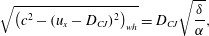 $$\begin{eqnarray}\sqrt{\left(c^{2}-(u_{x}-D_{CJ})^{2}\right)_{wh}}=D_{CJ}\sqrt{\frac{\unicode[STIX]{x1D6FF}}{\unicode[STIX]{x1D6FC}}},\end{eqnarray}$$
placing the wavehead at $y^{\ast }=2\unicode[STIX]{x1D70F}$
in our scaled coordinates. This is what we observe in all our simulations. Second, the signal at the wavehead is seen to decay with its increasing progress into the undisturbed 1-D detonation state (more evident in
$y^{\ast }=2\unicode[STIX]{x1D70F}$
in our scaled coordinates. This is what we observe in all our simulations. Second, the signal at the wavehead is seen to decay with its increasing progress into the undisturbed 1-D detonation state (more evident in ${\mathcal{V}}_{+}$
than in
${\mathcal{V}}_{+}$
than in ${\mathcal{U}}_{+}$
). The weakness of this wavehead, in what is a time-dependent, hyperbolic PDE system, is one of the reasons why a parabolic detonation propagation model that does not support a wavehead, like detonation shock dynamics, is able to describe the propagation of detonation fronts (see figure 6 and Bdzil & Stewart (Reference Bdzil and Stewart1986)).
${\mathcal{U}}_{+}$
). The weakness of this wavehead, in what is a time-dependent, hyperbolic PDE system, is one of the reasons why a parabolic detonation propagation model that does not support a wavehead, like detonation shock dynamics, is able to describe the propagation of detonation fronts (see figure 6 and Bdzil & Stewart (Reference Bdzil and Stewart1986)).
6.1.3 More loss of confinement:
$\unicode[STIX]{x1D6FF}=0.33$
with
${\mathcal{V}}_{bbc}=-2.0,-1.25,-1.1,\;-1.0$


As displayed in figure 12, when the streamline deflection angle decreases, the shock branch of the SRHR HE detonation shock polar becomes accessible. This translates to smaller values of $|{\mathcal{V}}_{bbc}|$
through (6.1). Next, we step through some different values of
$|{\mathcal{V}}_{bbc}|$
through (6.1). Next, we step through some different values of ${\mathcal{V}}_{bbc}$
, starting with
${\mathcal{V}}_{bbc}$
, starting with ${\mathcal{V}}_{bbc}=-2.0$
,
${\mathcal{V}}_{bbc}=-2.0$
, ${\mathcal{V}}_{bbc}=-1.25$
and then jumping to
${\mathcal{V}}_{bbc}=-1.25$
and then jumping to ${\mathcal{V}}_{bbc}=-1.0$
, to see how the growth of the shock/edge-intersection corner rarefaction fan is diminished and then stopped as
${\mathcal{V}}_{bbc}=-1.0$
, to see how the growth of the shock/edge-intersection corner rarefaction fan is diminished and then stopped as $|{\mathcal{V}}_{bbc}|$
is decreased. We end by examining the transitional case,
$|{\mathcal{V}}_{bbc}|$
is decreased. We end by examining the transitional case, ${\mathcal{V}}_{bbc}=-1.1$
, in some detail.
${\mathcal{V}}_{bbc}=-1.1$
, in some detail.
The ${\mathcal{U}}$
and
${\mathcal{U}}$
and ${\mathcal{V}}$
contours for the case with
${\mathcal{V}}$
contours for the case with ${\mathcal{V}}_{bbc}=-2.0$
are displayed in figures 13 and 14. As for the instantaneous reaction, the CJ case shown in figure 11, one finds both a rarefaction fan near the shock/edge-intersection corner and a smooth rarefaction near the left-hand side of both figures. The fan region is shown to grow backwards at a slower rate at
${\mathcal{V}}_{bbc}=-2.0$
are displayed in figures 13 and 14. As for the instantaneous reaction, the CJ case shown in figure 11, one finds both a rarefaction fan near the shock/edge-intersection corner and a smooth rarefaction near the left-hand side of both figures. The fan region is shown to grow backwards at a slower rate at $\unicode[STIX]{x1D70F}=30$
in figure 13 than in figure 11. The spatially resolved energy slows the growth of the fan region. However, as shown in figure 14, the fan eventually extends completely to the left boundary. This competition between energy removal by the fan and energy addition by the reaction is dominated in this case, by the fan. As the magnitude of the wall speed is reduced, there comes a point where the HEs resolved energy release will be dominant, as it is for a 1-D detonation. Reducing the magnitude of
$\unicode[STIX]{x1D70F}=30$
in figure 13 than in figure 11. The spatially resolved energy slows the growth of the fan region. However, as shown in figure 14, the fan eventually extends completely to the left boundary. This competition between energy removal by the fan and energy addition by the reaction is dominated in this case, by the fan. As the magnitude of the wall speed is reduced, there comes a point where the HEs resolved energy release will be dominant, as it is for a 1-D detonation. Reducing the magnitude of $|{\mathcal{V}}_{bbc}|$
to get
$|{\mathcal{V}}_{bbc}|$
to get ${\mathcal{V}}_{bbc}=-1.25$
, figure 20 shows the growth of the fan to be significantly retarded at
${\mathcal{V}}_{bbc}=-1.25$
, figure 20 shows the growth of the fan to be significantly retarded at $\unicode[STIX]{x1D70F}=30$
compared with what is observed in figures 13 and 15. Although the subsonic flow region in the
$\unicode[STIX]{x1D70F}=30$
compared with what is observed in figures 13 and 15. Although the subsonic flow region in the $\unicode[STIX]{x1D70F}=500~{\mathcal{U}}$
contour is nearly the same as that in figures 14 and 15, the supersonic flow shows that the shock/edge-intersection centred fan is all but absent, and the
$\unicode[STIX]{x1D70F}=500~{\mathcal{U}}$
contour is nearly the same as that in figures 14 and 15, the supersonic flow shows that the shock/edge-intersection centred fan is all but absent, and the ${\mathcal{U}}$
contours there more resemble those in a 1-D detonation reaction zone. The increasing role of the detonation heat release over the rarefaction fan in setting the detonation state is now clear.
${\mathcal{U}}$
contours there more resemble those in a 1-D detonation reaction zone. The increasing role of the detonation heat release over the rarefaction fan in setting the detonation state is now clear.

Figure 20. The ${\mathcal{U}}$
contours at
${\mathcal{U}}$
contours at $\unicode[STIX]{x1D70F}=30$
and
$\unicode[STIX]{x1D70F}=30$
and $\unicode[STIX]{x1D70F}=500$
for the case of the SRHR model with
$\unicode[STIX]{x1D70F}=500$
for the case of the SRHR model with $\unicode[STIX]{x1D6FF}=0.33$
,
$\unicode[STIX]{x1D6FF}=0.33$
, $k=0.02~\unicode[STIX]{x03BC}\text{s}^{-1}$
,
$k=0.02~\unicode[STIX]{x03BC}\text{s}^{-1}$
, $\unicode[STIX]{x1D708}=0.5$
, equation (2.5) parameters and
$\unicode[STIX]{x1D708}=0.5$
, equation (2.5) parameters and ${\mathcal{V}}_{bbc}=-1.25$
for the domain
${\mathcal{V}}_{bbc}=-1.25$
for the domain $-100\leqslant x^{\ast }\leqslant 0$
,
$-100\leqslant x^{\ast }\leqslant 0$
, $0\leqslant y^{\ast }\leqslant 110$
. Comparing the results here to those displayed in figures 13 and 15 for
$0\leqslant y^{\ast }\leqslant 110$
. Comparing the results here to those displayed in figures 13 and 15 for ${\mathcal{V}}_{bbc}=-2.0$
and
${\mathcal{V}}_{bbc}=-2.0$
and ${\mathcal{V}}_{bbc}=-4.0$
at
${\mathcal{V}}_{bbc}=-4.0$
at $\unicode[STIX]{x1D70F}=30$
, respectively, the strength and backward growth of the shock/edge-intersection centred fans are much reduced. The flow in the supersonic region at
$\unicode[STIX]{x1D70F}=30$
, respectively, the strength and backward growth of the shock/edge-intersection centred fans are much reduced. The flow in the supersonic region at $\unicode[STIX]{x1D70F}=500$
(the sonic locus is dashed) is not dominated by the fan, as it is in figures 14 and 15. The detonation heat release now even dominates the region of supersonic flow.
$\unicode[STIX]{x1D70F}=500$
(the sonic locus is dashed) is not dominated by the fan, as it is in figures 14 and 15. The detonation heat release now even dominates the region of supersonic flow.
Further reducing the speed of withdrawal of the bottom boundary to ${\mathcal{V}}_{bbc}=-1.0$
, finds that the role of the rarefaction fan is all but gone, and now the smooth rarefaction off of the bottom boundary is the dominant energy withdrawal mechanism competing with the HEs heat-release rate (see figure 21). The corner-centred supersonic rarefaction fan is barely visible. For
${\mathcal{V}}_{bbc}=-1.0$
, finds that the role of the rarefaction fan is all but gone, and now the smooth rarefaction off of the bottom boundary is the dominant energy withdrawal mechanism competing with the HEs heat-release rate (see figure 21). The corner-centred supersonic rarefaction fan is barely visible. For ${\mathcal{V}}_{bbc}=-4.0$
and
${\mathcal{V}}_{bbc}=-4.0$
and ${\mathcal{V}}_{bbc}=-2.0$
, the strength of the rarefaction fan exceeds the conditions necessary to establish a subsonic flow in the reaction zone. That is, the confinement is beyond a critical weakness and cannot influence the flow (as in the case of Lexan confinement shown in figure 12). For
${\mathcal{V}}_{bbc}=-2.0$
, the strength of the rarefaction fan exceeds the conditions necessary to establish a subsonic flow in the reaction zone. That is, the confinement is beyond a critical weakness and cannot influence the flow (as in the case of Lexan confinement shown in figure 12). For ${\mathcal{V}}_{bbc}=-1.0$
, the smooth rarefaction coming off of the bottom boundary directly sets the conditions of the flow in a reaction zone dominated by subsonic flow at
${\mathcal{V}}_{bbc}=-1.0$
, the smooth rarefaction coming off of the bottom boundary directly sets the conditions of the flow in a reaction zone dominated by subsonic flow at $\unicode[STIX]{x1D70F}=500$
. Near the edge of the explosive, now the competition between the explosive’s heat-release rate and the energy withdrawal by the smooth rarefaction is weighted in favour of the explosive’s heat-release rate.
$\unicode[STIX]{x1D70F}=500$
. Near the edge of the explosive, now the competition between the explosive’s heat-release rate and the energy withdrawal by the smooth rarefaction is weighted in favour of the explosive’s heat-release rate.

Figure 21. The ${\mathcal{U}}$
contours at
${\mathcal{U}}$
contours at $\unicode[STIX]{x1D70F}=30$
and
$\unicode[STIX]{x1D70F}=30$
and $\unicode[STIX]{x1D70F}=500$
for the case of the SRHR model with
$\unicode[STIX]{x1D70F}=500$
for the case of the SRHR model with $\unicode[STIX]{x1D6FF}=0.33$
,
$\unicode[STIX]{x1D6FF}=0.33$
, $k=0.02~\unicode[STIX]{x03BC}\text{s}^{-1}$
,
$k=0.02~\unicode[STIX]{x03BC}\text{s}^{-1}$
, $\unicode[STIX]{x1D708}=0.5$
, equation (2.5) parameters and
$\unicode[STIX]{x1D708}=0.5$
, equation (2.5) parameters and ${\mathcal{V}}_{bbc}=-1.0$
for the domain
${\mathcal{V}}_{bbc}=-1.0$
for the domain $-100\leqslant x^{\ast }\leqslant 0$
,
$-100\leqslant x^{\ast }\leqslant 0$
, $0\leqslant y^{\ast }\leqslant 110$
. The strength and reach of the shock/edge-intersection centred fan appears to be insignificant (see the insets of the corner-centred fan regions). Now, the sonic locus (shown as the dashed curve at
$0\leqslant y^{\ast }\leqslant 110$
. The strength and reach of the shock/edge-intersection centred fan appears to be insignificant (see the insets of the corner-centred fan regions). Now, the sonic locus (shown as the dashed curve at $\unicode[STIX]{x1D70F}=500$
) intersects the bottom boundary; although there is a barely visible supersonic region in the immediate vicinity of the corner in the
$\unicode[STIX]{x1D70F}=500$
) intersects the bottom boundary; although there is a barely visible supersonic region in the immediate vicinity of the corner in the $\unicode[STIX]{x1D70F}=500$
inset.
$\unicode[STIX]{x1D70F}=500$
inset.
This switch in dominance between energy addition by the explosive’s heat release and the energy withdrawal by the rarefaction is displayed in a plot of the steady-state detonation ( $\unicode[STIX]{x1D70F}=500$
) phase velocity
$\unicode[STIX]{x1D70F}=500$
) phase velocity $(-n)$
versus
$(-n)$
versus ${\mathcal{V}}_{bbc}$
in figure 22. The region where
${\mathcal{V}}_{bbc}$
in figure 22. The region where ${\mathcal{V}}_{bbc}<-1.25$
shows a constant propagation velocity which results when the detonation is fully unconfined.
${\mathcal{V}}_{bbc}<-1.25$
shows a constant propagation velocity which results when the detonation is fully unconfined.

Figure 22. The scaled, steady-state phase velocity, $(-n)$
, where
$(-n)$
, where $(D_{0}/D_{CJ})^{2}=1-\unicode[STIX]{x1D6FF}^{2}+\unicode[STIX]{x1D6FF}^{2}(1-n)$
, versus the bottom-boundary withdrawal speed,
$(D_{0}/D_{CJ})^{2}=1-\unicode[STIX]{x1D6FF}^{2}+\unicode[STIX]{x1D6FF}^{2}(1-n)$
, versus the bottom-boundary withdrawal speed, ${\mathcal{V}}_{bbc}$
, taken from the centreline at
${\mathcal{V}}_{bbc}$
, taken from the centreline at $\unicode[STIX]{x1D70F}=500$
. The SRHR model with (2.5) parameters,
$\unicode[STIX]{x1D70F}=500$
. The SRHR model with (2.5) parameters, $\unicode[STIX]{x1D6FF}=0.33$
,
$\unicode[STIX]{x1D6FF}=0.33$
, $k=0.02~\unicode[STIX]{x03BC}\text{s}^{-1}$
,
$k=0.02~\unicode[STIX]{x03BC}\text{s}^{-1}$
, $\unicode[STIX]{x1D708}=0.5$
, for the problem domain,
$\unicode[STIX]{x1D708}=0.5$
, for the problem domain, $-100\leqslant x^{\ast }\leqslant 0$
,
$-100\leqslant x^{\ast }\leqslant 0$
, $0\leqslant y^{\ast }\leqslant 110$
. The horizontal plateau, where
$0\leqslant y^{\ast }\leqslant 110$
. The horizontal plateau, where ${\mathcal{V}}_{bbc}\leqslant -1.25$
, corresponds to unconfined detonation.
${\mathcal{V}}_{bbc}\leqslant -1.25$
, corresponds to unconfined detonation.

Figure 23. The phase velocity, $\unicode[STIX]{x2202}\unicode[STIX]{x1D713}^{\ast }/\unicode[STIX]{x2202}\unicode[STIX]{x1D70F}=-n$
, along the edge (solid curve) and centreline (chain-dash curve) versus
$\unicode[STIX]{x2202}\unicode[STIX]{x1D713}^{\ast }/\unicode[STIX]{x2202}\unicode[STIX]{x1D70F}=-n$
, along the edge (solid curve) and centreline (chain-dash curve) versus $\unicode[STIX]{x1D70F}$
(a) and the
$\unicode[STIX]{x1D70F}$
(a) and the ${\mathcal{U}}$
contours at
${\mathcal{U}}$
contours at $\unicode[STIX]{x1D70F}=750$
(b), for the SRHR model with
$\unicode[STIX]{x1D70F}=750$
(b), for the SRHR model with $\unicode[STIX]{x1D6FF}=0.33$
,
$\unicode[STIX]{x1D6FF}=0.33$
, $k=0.02~\unicode[STIX]{x03BC}\text{s}^{-1}$
,
$k=0.02~\unicode[STIX]{x03BC}\text{s}^{-1}$
, $\unicode[STIX]{x1D708}=0.5$
, equation (2.5) parameters, for the domain
$\unicode[STIX]{x1D708}=0.5$
, equation (2.5) parameters, for the domain $-100\leqslant x^{\ast }\leqslant 0$
,
$-100\leqslant x^{\ast }\leqslant 0$
, $0\leqslant y^{\ast }\leqslant 110$
and for an impulsively withdrawn bottom boundary, with
$0\leqslant y^{\ast }\leqslant 110$
and for an impulsively withdrawn bottom boundary, with ${\mathcal{V}}_{bbc}=-1.1$
. In the transition from a fully unconfined detonation, with
${\mathcal{V}}_{bbc}=-1.1$
. In the transition from a fully unconfined detonation, with ${\mathcal{V}}_{bbc}=-1.25$
, and confined detonation with
${\mathcal{V}}_{bbc}=-1.25$
, and confined detonation with ${\mathcal{V}}_{bbc}=-1.0$
, a mixed steady state develops near the corner that has attributes of both unconfined and confined detonation. The flow displayed in (b) is steady at
${\mathcal{V}}_{bbc}=-1.0$
, a mixed steady state develops near the corner that has attributes of both unconfined and confined detonation. The flow displayed in (b) is steady at $\unicode[STIX]{x1D70F}=750$
and the dashed curves are sonic loci. The left boundary of the small supersonic region, embedded in the shock/edge-intersection corner of the otherwise subsonic region, and displayed in the inset, is a weak shock wave. We have seen the tent-shaped, inner supersonic flow near the boundary in transient flows in both other SRHR cases and for instantaneous reaction detonation. The structure displayed by the solid curve near
$\unicode[STIX]{x1D70F}=750$
and the dashed curves are sonic loci. The left boundary of the small supersonic region, embedded in the shock/edge-intersection corner of the otherwise subsonic region, and displayed in the inset, is a weak shock wave. We have seen the tent-shaped, inner supersonic flow near the boundary in transient flows in both other SRHR cases and for instantaneous reaction detonation. The structure displayed by the solid curve near $\unicode[STIX]{x1D70F}=150$
in (a) is the result of an earlier tent region being over washed by the return to the edge of the reflected wave off of the axis.
$\unicode[STIX]{x1D70F}=150$
in (a) is the result of an earlier tent region being over washed by the return to the edge of the reflected wave off of the axis.
The transition from a fully unconfined to a partially confined detonation occurs between $-1.25<{\mathcal{V}}_{bbc}<-1.0$
. As our last contour plot of a steady-state flow that can develop for the case
$-1.25<{\mathcal{V}}_{bbc}<-1.0$
. As our last contour plot of a steady-state flow that can develop for the case $\unicode[STIX]{x1D6FF}=0.33$
, equation (2.5) parameters,
$\unicode[STIX]{x1D6FF}=0.33$
, equation (2.5) parameters, $k=0.02~\unicode[STIX]{x03BC}\text{s}^{-1}$
and
$k=0.02~\unicode[STIX]{x03BC}\text{s}^{-1}$
and $\unicode[STIX]{x1D708}=0.5$
for the domain
$\unicode[STIX]{x1D708}=0.5$
for the domain $-100\leqslant x^{\ast }\leqslant 0$
,
$-100\leqslant x^{\ast }\leqslant 0$
, $0\leqslant y^{\ast }\leqslant 110$
, we show in figure 23(b) steady contours at
$0\leqslant y^{\ast }\leqslant 110$
, we show in figure 23(b) steady contours at $\unicode[STIX]{x1D70F}=750$
for the slowly evolving flow when
$\unicode[STIX]{x1D70F}=750$
for the slowly evolving flow when ${\mathcal{V}}_{bbc}=-1.1$
. Displayed in figure 23(a) are the phase velocity histories at the edge and centreline. For this transitional case, the phase velocities are only approaching steadiness at
${\mathcal{V}}_{bbc}=-1.1$
. Displayed in figure 23(a) are the phase velocity histories at the edge and centreline. For this transitional case, the phase velocities are only approaching steadiness at $\unicode[STIX]{x1D70F}\approx 500$
. We find an embedded region of supersonic flow, supporting a rarefaction fan, within an otherwise smooth, subsonic region of the reaction zone near the shock/edge-intersection corner. The flow shown in figure 23(b) is steady. There the left edge of the small supersonic region shown in the inset and sitting near the shock/edge-intersection corner is a shock wave. The evolution to steady state for this case is slow, owing to the broad regions near the lower boundary where the flow is nearly sonic (transonic). Flow structures of this type have been observed in special circumstances of high-speed flow past blunt bodies (Courant & Friedrichs Reference Courant and Friedrichs1948; von Mises Reference von Mises1958). Similar transition structures have been observed for a fully resolved reaction-zone model (Chiquete et al.
Reference Chiquete, Short, Meyer and Quirk2017).
$\unicode[STIX]{x1D70F}\approx 500$
. We find an embedded region of supersonic flow, supporting a rarefaction fan, within an otherwise smooth, subsonic region of the reaction zone near the shock/edge-intersection corner. The flow shown in figure 23(b) is steady. There the left edge of the small supersonic region shown in the inset and sitting near the shock/edge-intersection corner is a shock wave. The evolution to steady state for this case is slow, owing to the broad regions near the lower boundary where the flow is nearly sonic (transonic). Flow structures of this type have been observed in special circumstances of high-speed flow past blunt bodies (Courant & Friedrichs Reference Courant and Friedrichs1948; von Mises Reference von Mises1958). Similar transition structures have been observed for a fully resolved reaction-zone model (Chiquete et al.
Reference Chiquete, Short, Meyer and Quirk2017).
In the next section, we examine the properties of the steady-state flows that develop. There our attention will be directed at zones of influence and how information flows from the boundaries to set the detonation state.
7 Zones of influence in steady-state detonation flows: examples for
$\unicode[STIX]{x1D6FF}=0.33$
,
${\mathcal{V}}_{bbc}=-4.0$


Once the detonation flow becomes steady, equation (6.7),
 $$\begin{eqnarray}\frac{\unicode[STIX]{x2202}\unicode[STIX]{x1D6EF}}{\unicode[STIX]{x2202}x^{\ast }}\frac{\unicode[STIX]{x2202}^{2}\unicode[STIX]{x1D6EF}}{\unicode[STIX]{x2202}x^{\ast 2}}+\frac{\unicode[STIX]{x2202}^{2}\unicode[STIX]{x1D6EF}}{\unicode[STIX]{x2202}y^{\ast 2}}=\text{Rate},\end{eqnarray}$$
where $\unicode[STIX]{x1D6EF}$
is the velocity potential, describes the flow. Regions where
$\unicode[STIX]{x1D6EF}$
is the velocity potential, describes the flow. Regions where ${\mathcal{U}}=(\unicode[STIX]{x2202}\unicode[STIX]{x1D6EF}/\unicode[STIX]{x2202}x^{\ast })>0$
are subsonic and where
${\mathcal{U}}=(\unicode[STIX]{x2202}\unicode[STIX]{x1D6EF}/\unicode[STIX]{x2202}x^{\ast })>0$
are subsonic and where ${\mathcal{U}}=(\unicode[STIX]{x2202}\unicode[STIX]{x1D6EF}/\unicode[STIX]{x2202}x^{\ast })<0$
are supersonic, with
${\mathcal{U}}=(\unicode[STIX]{x2202}\unicode[STIX]{x1D6EF}/\unicode[STIX]{x2202}x^{\ast })<0$
are supersonic, with ${\mathcal{U}}=(\unicode[STIX]{x2202}\unicode[STIX]{x1D6EF}/\unicode[STIX]{x2202}x^{\ast })=0$
being the sonic locus. There is extensive literature (going back to the 1950s) on the required boundary data necessary to uniquely define solutions to this equation. This is largely due to its being possible to transform (7.1) to a linear PDE, by interchanging the independent and dependent variables, using the Hodograph transformation (Courant & Friedrichs Reference Courant and Friedrichs1948). Here, we use that theory to set out the appropriate set of boundary curves and data domains of dependence with which to uniquely define our detonation flows.
${\mathcal{U}}=(\unicode[STIX]{x2202}\unicode[STIX]{x1D6EF}/\unicode[STIX]{x2202}x^{\ast })=0$
being the sonic locus. There is extensive literature (going back to the 1950s) on the required boundary data necessary to uniquely define solutions to this equation. This is largely due to its being possible to transform (7.1) to a linear PDE, by interchanging the independent and dependent variables, using the Hodograph transformation (Courant & Friedrichs Reference Courant and Friedrichs1948). Here, we use that theory to set out the appropriate set of boundary curves and data domains of dependence with which to uniquely define our detonation flows.
In supersonic regions of the flow, our boundary condition discussion involves two families of characteristics
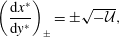 $$\begin{eqnarray}\left(\frac{\text{d}x^{\ast }}{\text{d}y^{\ast }}\right)_{\pm }=\pm \sqrt{-{\mathcal{U}}},\end{eqnarray}$$
which represent the paths along which information flows from and to the boundaries. This includes how information moves from the confinement boundary to the sonic locus for an unconfined detonation. Then the steady-state SRHR model, (7.1), can be written as a pair of ordinary differential equations along the paths given by (7.2)
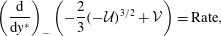 $$\begin{eqnarray}\displaystyle & \displaystyle \left(\frac{\text{d}}{\text{d}y^{\ast }}\right)_{-}\left(-\frac{2}{3}(-{\mathcal{U}})^{3/2}+{\mathcal{V}}\right)=\text{Rate}, & \displaystyle\end{eqnarray}$$
 $$\begin{eqnarray}\displaystyle & \displaystyle \left(\frac{\text{d}}{\text{d}y^{\ast }}\right)_{+}\left(\frac{2}{3}(-{\mathcal{U}})^{3/2}+{\mathcal{V}}\right)=\text{Rate}, & \displaystyle\end{eqnarray}$$
and where
 $$\begin{eqnarray}\left(\frac{\text{d}}{\text{d}y^{\ast }}\right)_{\pm }=\pm \sqrt{-{\mathcal{U}}}\frac{\unicode[STIX]{x2202}\;}{\unicode[STIX]{x2202}x^{\ast }}+\frac{\unicode[STIX]{x2202}\;}{\unicode[STIX]{x2202}y^{\ast }}.\end{eqnarray}$$
In figure 15 we saw that for an unconfined detonation, a broad supersonic region separated the bottom confinement boundary from the subsonic region of the reaction-zone flow. Thus details on how information moves through this supersonic region to the sonic locus is important to connect how the confinement boundary influences such features as the shape and speed of the detonation shock, both of which are intimately tied to the region of subsonic flow.
We turn to the classic example for 2-D, steady flows of mixed hyperbolic (supersonic) and elliptic (subsonic) types, the Tricomi equation (Guderley Reference Guderley1962), to precisely formulate what boundary curves and data are appropriate for our detonation problem to have the solution be uniquely defined. Those who have studied quasi-1-D and quasi-steady 2-D detonation know of the central role of the sonic locus in setting the detonation speed as part of the solution of the detonation-eigenvalue problem (Fickett & Davis Reference Fickett and Davis1979, pp. 133–229). Although the sonic locus continues to divide subsonic from supersonic flows, because of the complex shape of this locus (with the sonic locus intersecting the shock), then since the characteristics can squarely intersect the sonic locus, the information they carry will be deposited on that locus. Here our discussion follows Guderley’s for a related problem, flow in a de Laval nozzle containing a sharp corner (Guderley Reference Guderley1962). The reader is referred to figure 41 in Guderley (Reference Guderley1962) for the discussion. Here we borrow points from his discussion and apply them to our flow.
Displayed in figure 24 is the laboratory coordinate representation of the steady-state solution of the SRHR detonation for $\unicode[STIX]{x1D6FF}=0.33$
,
$\unicode[STIX]{x1D6FF}=0.33$
, $k=0.02~\unicode[STIX]{x03BC}\text{s}^{-1}$
,
$k=0.02~\unicode[STIX]{x03BC}\text{s}^{-1}$
, $\unicode[STIX]{x1D708}=0.5$
, equation (2.5) parameters with
$\unicode[STIX]{x1D708}=0.5$
, equation (2.5) parameters with ${\mathcal{V}}_{bbc}=-4.0$
and solved on the domain
${\mathcal{V}}_{bbc}=-4.0$
and solved on the domain $-100\leqslant x^{\ast }\leqslant 0$
,
$-100\leqslant x^{\ast }\leqslant 0$
, $0\leqslant y^{\ast }\leqslant 110$
. Following Guderley (Reference Guderley1962), data must be prescribed on three curves to uniquely define the steady-state solution: (i) along the detonation shock (the shock conditions), (ii) along the centreline (the symmetry condition) and (iii) along a cross-characteristic encircling the fan singularity, starting at the sonic locus and ending at the limiting characteristic. The limiting characteristic (displayed as the chain-dashed curve) is the characteristic emanating from the fan singularity that is just tangent to the sonic locus (dashed curve) at the centreline. The data along the second family of characteristics, the cross-characteristics, define the fan singularity. These data are carried back and upwards by the first family of characteristics that sits to the right of the limiting characteristic, and is squarely deposited onto the sonic locus.
$0\leqslant y^{\ast }\leqslant 110$
. Following Guderley (Reference Guderley1962), data must be prescribed on three curves to uniquely define the steady-state solution: (i) along the detonation shock (the shock conditions), (ii) along the centreline (the symmetry condition) and (iii) along a cross-characteristic encircling the fan singularity, starting at the sonic locus and ending at the limiting characteristic. The limiting characteristic (displayed as the chain-dashed curve) is the characteristic emanating from the fan singularity that is just tangent to the sonic locus (dashed curve) at the centreline. The data along the second family of characteristics, the cross-characteristics, define the fan singularity. These data are carried back and upwards by the first family of characteristics that sits to the right of the limiting characteristic, and is squarely deposited onto the sonic locus.

Figure 24. The problem domain for the steady-state SRHR model detonation solution, displayed in laboratory coordinates. The problem parameters are those given in the caption to figure 15. A unique solution is obtained given data along curve 1, the shock conditions, along curve 2, the symmetry condition and along curve 3, a cross-characteristic encircling the rarefaction fan in the supersonic region of the shock/edge-intersection corner. Also shown are characteristics emanating from the rarefaction-fan singularity and the sonic locus (dashed curve). The characteristic emanating from the fan singularity and just tangent to the sonic locus at the centreline (shown as the chain-dashed curve) is called the limiting characteristic. Only characteristics emanating from the fan singularity and to the right of the limiting characteristic deposit information on the sonic locus, and as a result, influence the subsonic zone. The data propagated along these characteristics can affect the speed and shape of the detonation shock.
The role of the shock and symmetry boundary conditions in defining the solution is clear. Here we focus on the data for $(-\frac{2}{3}(-{\mathcal{U}})^{3/2}+{\mathcal{V}})$
along the cross-characteristic, a member of the second family of characteristics (curve 3 in figure 24). As we integrate (7.3) through the supersonic region along the first family of characteristics, starting at the cross-characteristic and ending at the sonic locus, then the magnitude of the
$(-\frac{2}{3}(-{\mathcal{U}})^{3/2}+{\mathcal{V}})$
along the cross-characteristic, a member of the second family of characteristics (curve 3 in figure 24). As we integrate (7.3) through the supersonic region along the first family of characteristics, starting at the cross-characteristic and ending at the sonic locus, then the magnitude of the $\text{Rate}$
along that characteristic paths increases
$\text{Rate}$
along that characteristic paths increases $(-\frac{2}{3}(-{\mathcal{U}})^{3/2}+{\mathcal{V}})$
, until we get to the sonic locus where
$(-\frac{2}{3}(-{\mathcal{U}})^{3/2}+{\mathcal{V}})$
, until we get to the sonic locus where ${\mathcal{U}}=0$
and the accumulated value of
${\mathcal{U}}=0$
and the accumulated value of ${\mathcal{V}}$
is deposited along the sonic locus. In a similar fashion, data on
${\mathcal{V}}$
is deposited along the sonic locus. In a similar fashion, data on $(\frac{2}{3}(-{\mathcal{U}})^{3/2}+{\mathcal{V}})$
taken from along the sonic locus are integrated with (7.4) along the paths of the second family of characteristics towards the bottom boundary, decreasing
$(\frac{2}{3}(-{\mathcal{U}})^{3/2}+{\mathcal{V}})$
taken from along the sonic locus are integrated with (7.4) along the paths of the second family of characteristics towards the bottom boundary, decreasing $(\frac{2}{3}(-{\mathcal{U}})^{3/2}+{\mathcal{V}})$
until the bottom boundary is reached. Then with
$(\frac{2}{3}(-{\mathcal{U}})^{3/2}+{\mathcal{V}})$
until the bottom boundary is reached. Then with ${\mathcal{V}}$
known on that boundary, the value of
${\mathcal{V}}$
known on that boundary, the value of ${\mathcal{U}}$
is deposited on that boundary. So information from both the fan singularity and the supersonic region, between the bottom boundary and the sonic locus (including information on the
${\mathcal{U}}$
is deposited on that boundary. So information from both the fan singularity and the supersonic region, between the bottom boundary and the sonic locus (including information on the $\text{Rate}$
), is deposited on the sonic locus not only affecting the shape of the sonic locus but also such quantities as the detonation phase velocity that are determined in the subsonic zone.
$\text{Rate}$
), is deposited on the sonic locus not only affecting the shape of the sonic locus but also such quantities as the detonation phase velocity that are determined in the subsonic zone.
The relative importance of this supersonic region to the flow in the subsonic region is a function of the lateral dimension of the explosive charge size. The larger the distance to the symmetry line (the wider the charge size), the less is the effect of this supersonic region on the subsonic region, and on such quantities as the shock shape and the detonation phase velocity.
From the above discussion, it should be clear that the characteristics that intersect the sonic locus will be influenced by the flow in the region they traverse, including information about the $\text{Rate}$
and EOS. Here we describe how information about the boundary condition along the bottom of our domain, as represented by
$\text{Rate}$
and EOS. Here we describe how information about the boundary condition along the bottom of our domain, as represented by ${\mathcal{V}}_{bbc}$
, can influence the solution in the subsonic region. This more quantitative discussion will focus on the transition in detonation response, as displayed in figures 20 and 23, and on why the rarefaction fan recedes towards the corner as we decrease the magnitude of
${\mathcal{V}}_{bbc}$
, can influence the solution in the subsonic region. This more quantitative discussion will focus on the transition in detonation response, as displayed in figures 20 and 23, and on why the rarefaction fan recedes towards the corner as we decrease the magnitude of ${\mathcal{V}}_{bbc}$
.
${\mathcal{V}}_{bbc}$
.
Displayed in figure 25(a) is a blowup of the steady-state solution for the problem described in the caption to figure 15. Shown are the members of the first family of characteristics, shock, sonic locus and the limiting characteristic, all displayed in shock-attached coordinates. Figure 25(b) shows the shock polar displayed in figure 12, now with the inclusion of the ‘limiting characteristic point’. This point corresponds to the pressure on the limiting characteristics in the corner. For the detonation to propagate at the speed of a fully unconfined detonation, the inert material providing confinement must cross the SRHR-fan polar below the ‘limiting characteristic point’. In the event that the polar of the confining inert material crosses above this point, the rarefaction fan would be narrowed, with the characteristics emanating from the fan singularity not being able to reach the entirety of the sonic locus. This would disrupt the steady, unconfined solution. The likely outcome of this disruption would be a flow like that pictured in figure 23. As the confinement becomes even stronger, we would then transition the shock-polar solution to the SRHR shock branch, as displayed for the tungsten example in figure 12.

Figure 25. (a) Shows an expanded view (in shock-attached coordinates) of the vicinity of the shock/edge-intersection corner for the characteristic diagram (in laboratory coordinates) displayed in figure 24. The limiting characteristic, sonic locus and a number of other characteristics are shown. The $P=25.66~\text{GPa}$
contour is tangent to the limiting characteristic at the corner. (b) Shows the shock-polar diagram displayed in figure 12. The point labelled as ‘limiting characteristic point’ corresponds to the pressure on the limiting characteristic at the corner in (a). In order for the unconfined detonation displayed here to remain unconfined, the shock polar for the inert material (the Lexan polar here) must cross the SRHR fan below the ‘limiting characteristic point’.
$P=25.66~\text{GPa}$
contour is tangent to the limiting characteristic at the corner. (b) Shows the shock-polar diagram displayed in figure 12. The point labelled as ‘limiting characteristic point’ corresponds to the pressure on the limiting characteristic at the corner in (a). In order for the unconfined detonation displayed here to remain unconfined, the shock polar for the inert material (the Lexan polar here) must cross the SRHR fan below the ‘limiting characteristic point’.
The quantitative discussion presented here allows us to understand the phase velocity versus confinement ( ${\mathcal{V}}_{bbc}$
) curve displayed in figure 22. In addition, the limiting characteristic diagram (figures 24 and 25) provides some insights into why the rarefaction fan shrinks into the corner when the magnitude of
${\mathcal{V}}_{bbc}$
) curve displayed in figure 22. In addition, the limiting characteristic diagram (figures 24 and 25) provides some insights into why the rarefaction fan shrinks into the corner when the magnitude of ${\mathcal{V}}_{bbc}$
is decreased. Going on to consider the case for
${\mathcal{V}}_{bbc}$
is decreased. Going on to consider the case for ${\mathcal{V}}_{bbc}=-1.0$
, that is displayed in figure 21, the fan at the shock/edge-intersection corner is essentially absent, and the sonic locus, which now intersects the bottom boundary, both sits well back from the shock and is followed by what is a non-singular, distributed shallow ‘fan’. These characteristic paths propagate both to the sonic locus and far back into the following flow (see figure 26). The influence of the supersonic region behind the sonic locus and along the wall on the subsonic region, is now much weaker than what is displayed in figure 25. This is due to the shorter characteristic paths and how close the characteristic paths that intersect the sonic locus stay to the sonic locus. The shorter distances travelled along these characteristic paths lessens the ability of the reactivity there to influence the subsonic region. Thus, as the strength of the confinement increases (this corresponds to
${\mathcal{V}}_{bbc}=-1.0$
, that is displayed in figure 21, the fan at the shock/edge-intersection corner is essentially absent, and the sonic locus, which now intersects the bottom boundary, both sits well back from the shock and is followed by what is a non-singular, distributed shallow ‘fan’. These characteristic paths propagate both to the sonic locus and far back into the following flow (see figure 26). The influence of the supersonic region behind the sonic locus and along the wall on the subsonic region, is now much weaker than what is displayed in figure 25. This is due to the shorter characteristic paths and how close the characteristic paths that intersect the sonic locus stay to the sonic locus. The shorter distances travelled along these characteristic paths lessens the ability of the reactivity there to influence the subsonic region. Thus, as the strength of the confinement increases (this corresponds to $|{\mathcal{V}}_{bbc}|$
decreasing), and we go from the case of figures 24 and 25 to that of figure 26, the influence of the supersonic region on the subsonic region, and everything that the subsonic region determines, is diminished. Restated somewhat differently, either as the confinement increases and the area of supersonic region that can influence the subsonic region diminishes (as in going from figures 24 and 26) or as the explosive charge size for an unconfined detonation increases, and the supersonic flow near the corner is proportionately a smaller influence, then the classical picture of the dominant role of the subsonic region becomes closer to correct. The important role of the supersonic region in setting the sonic locus and boundary conditions for the subsonic region, by depositing data along the sonic locus (as displayed in figure 24), should not be under appreciated. The sharp break in the detonation speed versus confinement curve, displayed in figure 22, is witness to the important role of the singular rarefaction fan on confinement and how sharply the detonation speed changes as the rarefaction fan gives way to a smooth release. Based on the above discussion, the steady-state detonation displayed in figure 20(b) is unconfined, while that displayed in figure 23(b) is a hybrid, partially confined case.
$|{\mathcal{V}}_{bbc}|$
decreasing), and we go from the case of figures 24 and 25 to that of figure 26, the influence of the supersonic region on the subsonic region, and everything that the subsonic region determines, is diminished. Restated somewhat differently, either as the confinement increases and the area of supersonic region that can influence the subsonic region diminishes (as in going from figures 24 and 26) or as the explosive charge size for an unconfined detonation increases, and the supersonic flow near the corner is proportionately a smaller influence, then the classical picture of the dominant role of the subsonic region becomes closer to correct. The important role of the supersonic region in setting the sonic locus and boundary conditions for the subsonic region, by depositing data along the sonic locus (as displayed in figure 24), should not be under appreciated. The sharp break in the detonation speed versus confinement curve, displayed in figure 22, is witness to the important role of the singular rarefaction fan on confinement and how sharply the detonation speed changes as the rarefaction fan gives way to a smooth release. Based on the above discussion, the steady-state detonation displayed in figure 20(b) is unconfined, while that displayed in figure 23(b) is a hybrid, partially confined case.

Figure 26. For the confined detonation case of figure 21, here we show how the characteristics that both end at the sonic locus and travel far back into the flow come from a distributed, shallow ‘fan’ that starts where the bottom boundary meets the sonic locus. An expanded view of the region behind the sonic locus is displayed in the inset.
8 Summary
In this paper, which is a companion to Bdzil & Short (Reference Bdzil and Short2017), we have considered the problem of detonation confinement, for the case where a compliant inert material along the detonating explosive’s boundary, is deflected by the passage of the detonation. This leads to the propagation of a rarefaction into the explosive’s detonation reaction zone. Here we have modelled that problem with a boundary condition which prescribes the constant, velocity of withdrawal of the boundary, once the detonation passes. This is accomplished by solving the problem in a shock-attached reference frame, which makes applying such a boundary condition straightforward. Since the shock corresponds to one boundary and the deflected interface to another, we enjoy the advantage of not having the numerical errors associated with either shock-capturing or material interface algorithms.
With these advantages, we are able to study the singular flows that develop at the point where the shock and boundary meet, resulting from the abrupt, scale-free withdrawal of the boundary. To reduce some of the complexity of the fully resolved, reaction-zone model, here we use the SRHR detonation model, which considers a 2-step, reaction-kinetics model, and focuses on how the last 10 % of the explosive’s energy release influences a 2-D detonation flow. With this model, we can reduce the problem to the unsteady, transonic, small-disturbance equation, with an added source term to model the resolved detonation energy release. This nonlinear, 2-D model captures the transonic flow which dominates unsupported detonation propagation. We solved the modelling equations using the implicit, finite-difference solver described in § 3.1: a solver related to the Murman–Cole solver (Murman & Cole Reference Murman and Cole1971).
We studied both the time-dependent, full instantaneous reaction, CJ and the partially resolved reaction, SRHR detonation models. There are two features that the solutions to both models have in common: (i) a singular rarefaction fan, centred at the shock/edge-intersection corner and (ii) a smooth rarefaction moving up from the full length of the withdrawn bottom boundary. For the CJ detonation case, the singular fan sits in a region of supersonic flow, while the smooth rarefaction is found in a region of subsonic flow. In the competition between these two rarefactions, the singular fan wins in the end, independent of the strength of the rarefaction. For the SRHR detonation, there is another player: the spatially resolved energy release. Now, the resolved energy release can suppress the fan, and we can end with a steady, subsonic flow in the shock/edge-intersection corner when the rarefaction is not of sufficient strength. This transition in steady-state SRHR detonation confinement response occurs near ${\mathcal{V}}_{bbc}=-1.1$
, when (2.5) parameters are used. Solutions with
${\mathcal{V}}_{bbc}=-1.1$
, when (2.5) parameters are used. Solutions with ${\mathcal{V}}_{bbc}\leqslant -1.25$
yield unconfined fan solutions while solutions with
${\mathcal{V}}_{bbc}\leqslant -1.25$
yield unconfined fan solutions while solutions with ${\mathcal{V}}_{bbc}\geqslant -1.0$
yield confined smooth solutions. In the transition region,
${\mathcal{V}}_{bbc}\geqslant -1.0$
yield confined smooth solutions. In the transition region, $-1.0<{\mathcal{V}}_{bbc}<-1.25$
, the solutions are mixed, including both fan and smooth features along the confinement boundary (see figure 23
b).
$-1.0<{\mathcal{V}}_{bbc}<-1.25$
, the solutions are mixed, including both fan and smooth features along the confinement boundary (see figure 23
b).
When examined on a finer-grained scale, we have the following specific takeaways for the detonation confinement problem:
-
(i) Our SRHR results are valid for
$\sqrt{(1-n)_{CL}}=A\unicode[STIX]{x1D6FF}^{1/2}$
, achieved in explosives of a moderate half-width size (approximately 5), measured on the reaction-zone scale (see figure 6). -
(ii) The impulsive removal of the confinement boundary, causes the detonation phase velocity at the edge to first experience an abrupt decrease. This early-time evolution for a SRHR detonation is controlled by a reaction-rate-independent, self-similar, initial-boundary value problem, for which the initial state is the ZND shock state. Sonic loci can be defined for this early-time flow. At later times, the phase velocity at the edge increases as the interaction of the rarefaction with the explosive’s heat-release rate plays out.
-
(iii) For unconfined SRHR explosive charges, those with
${\mathcal{V}}_{bbc}\leqslant -1.25$
for (2.5) parameters, the flow is found to have
${\mathcal{U}}_{+}(\,y^{\ast }=0,\unicode[STIX]{x1D70F})=0$
, which could be interpreted as sonic at the charge edge, for all
$\unicode[STIX]{x1D70F}>0$
, as measured in a reference frame moving along with the shock/edge-intersection point. This corresponds to the minimum allowed normal detonation velocity,
$D_{n}^{2}=D_{CJ}^{2}(1-\unicode[STIX]{x1D6FF}^{2})$
, and shock pressure for a SRHR detonation. -
(iv) The last two points are consistent with the sonic constraint of (1.6) at the edge.
-
(v) As the rarefaction wavehead propagates through the reaction zone, its amplitude where it intersects the shock decays to low levels.
-
(vi) As displayed in figures 19 and 23(a), the phase velocity takes a long time to reach steadiness, with transients exhibiting undershoots and overshoots.
-
(vii) Once the full steady state is reached, we can more generally describe the flow as subsonic and supersonic over the entire flow field. In the steady limit, a sonic locus is established in the reaction zone, that intersects the shock/edge-intersection corner for weak confinement and the confinement boundary for strong confinement.
-
(viii) For a steady SRHR detonation, there exists in the supersonic region a limiting characteristic which separates what is a fully unconfined detonation from a partially confined detonation (see figure 25 and the surrounding discussion).
-
(ix) For a fully unconfined, steady-state detonation, a significant part of the supersonic flow region near the confinement boundary can influence the solution in the subsonic part of the reaction zone. The degree to which the subsonic zone is influenced depends on the lateral dimension (width) of the explosive charge, with wider charges being less affected.
-
(x) For a well-confined but still 2-D detonation, the trailing supersonic region of the reaction zone only weakly affects the subsonic region of the reaction zone.
-
(xi) Taken together, the last two points support the notion discussed in Fickett & Davis (Reference Fickett and Davis1979, pp. 133–229) of an eigenvalue detonation for setting the speed of a steady-detonation wave, when the lateral dimension of the detonation charge is many reaction-zone lengths wide.


As a general remark, we expect results of our SRHR model study to provide a qualitative picture of what to expect for the fully resolved, reaction-zone model problem in many instances. Some results that we have been able to compare against, such as those of Romick & Aslam (Reference Romick and Aslam2017) and Chiquete et al. (Reference Chiquete, Short, Meyer and Quirk2017), show such agreement. The solutions of the SRHR, UTSD equations that we have shown here, capture the transonic flow that controls the slow evolution of unsupported detonation to a 2-D steady flow.
In closing, we note that the SRHR model differs from the more widely studied small heat-release model in one significant respect: the form of the shock conditions. Equation (8.1) is the shock condition (restricted to semi-infinite charges, see (6.18)) for the SRHR model, and (8.2) is the shock condition for the small heat-release model (Faria, et al. Reference Faria, Kasimov and Rosales2015),
 $$\begin{eqnarray}\displaystyle & \displaystyle \frac{\unicode[STIX]{x2202}\unicode[STIX]{x1D713}_{s}^{\ast }}{\unicode[STIX]{x2202}\unicode[STIX]{x1D70F}}=-1+{\mathcal{U}}_{+}^{2}+\unicode[STIX]{x1D6FF}\unicode[STIX]{x1D6FC}\left(\frac{\unicode[STIX]{x2202}\unicode[STIX]{x1D713}_{s}^{\ast }}{\unicode[STIX]{x2202}y^{\ast }}\right)^{2}+\cdots \,, & \displaystyle\end{eqnarray}$$
 $$\begin{eqnarray}\displaystyle & \displaystyle \frac{\unicode[STIX]{x2202}\unicode[STIX]{x1D713}_{s}}{\unicode[STIX]{x2202}t}=\frac{\unicode[STIX]{x1D70E}_{+}+\unicode[STIX]{x1D70E}_{0}}{2}+\left(\frac{\unicode[STIX]{x2202}\unicode[STIX]{x1D713}_{s}}{\unicode[STIX]{x2202}y}\right)^{2}, & \displaystyle\end{eqnarray}$$
where here $\unicode[STIX]{x1D70E}$
is the flow variable in the small heat-release model which corresponds to
$\unicode[STIX]{x1D70E}$
is the flow variable in the small heat-release model which corresponds to ${\mathcal{U}}$
in the SRHR model. The quadratic dependence of (8.1) on
${\mathcal{U}}$
in the SRHR model. The quadratic dependence of (8.1) on ${\mathcal{U}}$
limits the shock speed,
${\mathcal{U}}$
limits the shock speed, $(\unicode[STIX]{x2202}\unicode[STIX]{x1D713}_{s}^{\ast }/\unicode[STIX]{x2202}\unicode[STIX]{x1D70F})$
, to a minimum velocity, associated with the instantaneous energy-release fraction of the SRHR detonation. The linear dependence of (8.2) on
$(\unicode[STIX]{x2202}\unicode[STIX]{x1D713}_{s}^{\ast }/\unicode[STIX]{x2202}\unicode[STIX]{x1D70F})$
, to a minimum velocity, associated with the instantaneous energy-release fraction of the SRHR detonation. The linear dependence of (8.2) on $\unicode[STIX]{x1D70E}$
provides no such downside limiting of the shock velocity for the small heat-release model. In our earlier study of Mach reflection for a CJ-limit detonation (Bdzil & Short Reference Bdzil and Short2017), we found a smoothly curved Mach-reflection shock, independent of the angle of attack of the incident detonation. That self-similar solution showed the flow cleanly separated into a supersonic region ahead of the reflected shock and behind the incident shock and a subsonic region bounded by the reflected shock, the curved Mach shock and the bottom boundary. The problem of inert material, weak shock reflection shares properties with this CJ-detonation problem, including the UTSD equations, with (8.2) replacing (8.1) (Tesdall & Hunter Reference Tesdall and Hunter2002). Unlike the smooth flow we see behind the Mach shock for the SRHR model, simulations for this inert flow reveal small supersonic regions, attached to the Mach shock and embedded in the mostly subsonic flow behind it (Hunter & Brio Reference Hunter and Brio2000). These regions contain weak shocks followed by fans. Although controversy remains concerning these localized shock-fan complexes, it is interesting that the CJ-limit, SRHR detonation does not exhibit such structures (Bdzil & Short Reference Bdzil and Short2017).
$\unicode[STIX]{x1D70E}$
provides no such downside limiting of the shock velocity for the small heat-release model. In our earlier study of Mach reflection for a CJ-limit detonation (Bdzil & Short Reference Bdzil and Short2017), we found a smoothly curved Mach-reflection shock, independent of the angle of attack of the incident detonation. That self-similar solution showed the flow cleanly separated into a supersonic region ahead of the reflected shock and behind the incident shock and a subsonic region bounded by the reflected shock, the curved Mach shock and the bottom boundary. The problem of inert material, weak shock reflection shares properties with this CJ-detonation problem, including the UTSD equations, with (8.2) replacing (8.1) (Tesdall & Hunter Reference Tesdall and Hunter2002). Unlike the smooth flow we see behind the Mach shock for the SRHR model, simulations for this inert flow reveal small supersonic regions, attached to the Mach shock and embedded in the mostly subsonic flow behind it (Hunter & Brio Reference Hunter and Brio2000). These regions contain weak shocks followed by fans. Although controversy remains concerning these localized shock-fan complexes, it is interesting that the CJ-limit, SRHR detonation does not exhibit such structures (Bdzil & Short Reference Bdzil and Short2017).
Acknowledgements
This work was presented in part at the 26th ICDERS, July 30th–August 4th 2017, Boston, MA. We thank W. C. Davis for his support of work on detonation theory at Los Alamos through the years. The comments made by the referees led to improvements to our paper.


 Open access