


Impact Statement
The evolution of sediment plumes is a multiscale and multiphysics process of great complexity that plays a key role in setting the indirect impact of deep-sea mining activities. Most recent efforts to model such plumes have relied on large-scale numerical simulations of specific operational parameters over time scales that are much smaller than the typical duration of an operation. As a result, considerable uncertainty remains as to the role played by key physical oceanography and operational parameters on setting the extent of plumes. In addition, the very definition of the extent metric of interest plays a foundational role in setting the scale of the impact of plumes. The work presented herein takes a more fundamental simplified approach that aims at gaining a first-order understanding of the extent of sediment plumes over long time scales, and how the key parameters affect their extent. The findings can guide future efforts to characterize impact and inform future research.
1. Introduction
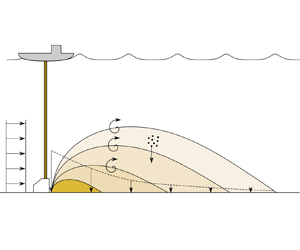
Deep-sea nodule mining is a nascent industry that involves the physical collection of polymetallic nodules – small fist-sized rocks that contain large quantities of various metals – found in abundance on the seafloor in certain regions of the deep ocean. One of the main environmental concerns associated with deep-sea nodule mining is the two types of sediment plumes that would be created, a so-called midwater plume and a so-called collector plume. A midwater plume originates from the discharge of sediment that was brought up to the processing ship along with the nodules via a vertical transport system, and that is returned to the water column at some depth below the surface, expected to be 1000 m or deeper and well above the seabed (Reference Muñoz-Royo, Peacock, Alford, Smith, Le Boyer, Kulkarni and JuMuñoz-Royo et al., 2021). The collector plume is generated by the discharge of resuspended sediment in the direct vicinity of a collector vehicle, likely in its wake (see figure 1), and is the focus of this paper. While there are similarities between midwater and collector plumes, the presence of the seabed markedly affects the behaviour of the plume. Indeed, as the plume evolves close to the seabed from its inception, progressive deposition plays a central role in controlling the evolution of the collector plume, the amount of sediment in suspension, the total extent of the plume and a fortiori its potential environmental impact.

Figure 1. Sketch of the vertical slice of the collector plume (not to scale). Advection acts to transport sediment away from the mining area. Vertical turbulent diffusion acts to transport sediment upwards, and opposes settling which acts to transport sediment towards the seabed.
Early efforts to characterize the evolution of a collector plume immediately after release raised the prospect that the negative buoyancy of the sediment-laden mixture discharged behind the vehicle will initially drive the spreading of the plume (Reference Jankowski, Malcherek and ZielkeJankowski, Malcherek, & Zielke, 1996; Reference Lavelle, Ozturgut, Swift and EricksonLavelle, Ozturgut, Swift, & Erickson, 1981; Reference Ouillon, Kakoutas, Meiburg and PeacockOuillon, Kakoutas, Meiburg, & Peacock, 2021; Reference Rutkowska, Dubalska, Bajger-Nowak, Konieczka and NamieśnikRutkowska, Dubalska, Bajger-Nowak, Konieczka, & Namieśnik, 2014). This assertion was confirmed during recent collector trials in the Clarion Clipperton Fracture Zone (CCFZ) by the first-of-their-kind experiments of Reference Muñoz-Royo, Ouillon, El Mousadik, Alford and PeacockMuñoz-Royo, Ouillon, El Mousadik, Alford, and Peacock (in press), which made the first direct observations of the turbidity current dynamics released during test nodule mining operations. Reference Muñoz-Royo, Ouillon, El Mousadik, Alford and PeacockMuñoz-Royo et al. (in press) argued that a combination of turbulent mixing in the wake of the collector and detrainment of fine sediment from the turbidity current generated by the discharge sets the initial conditions for the collector ambient plume, i.e. the initial distribution of sediment that is made available for far-field transport by background currents, which is what was observed in the numerical modelling and laboratory experiments of Reference Ouillon, Kakoutas, Meiburg and PeacockOuillon et al. (2021).
Most efforts to numerically model the evolution of the collector ambient plume have relied on hydrostatic or non-hydrostatic formulations of the momentum equations to describe the flow field, and then solved the advection–diffusion equation for a concentration scalar (Reference Aleynik, Inall, Dale and VinkAleynik, Inall, Dale, & Vink, 2017; Reference Jankowski, Malcherek and ZielkeJankowski et al., 1996). In these approaches, the equations need to be integrated over long times and large horizontal distances, resulting in constraints on feasible grid sizing that can be resolved at acceptable computational costs. This is particularly problematic when considering vertical gradients of sediment concentration close to the seabed, where vertical eddy diffusivities of  $O(10^{-4}-10^{-2})$ m $^{2}$ s $^{-1}$ are expected (Reference Aleynik, Inall, Dale and VinkAleynik et al., 2017; Reference van Harenvan Haren, 2018). The collector plume following the turbidity current phase is typically a few metres thick, and observations of the collector plume after several hours suggest that sharp gradients of concentration are maintained over significant time scales (Reference Muñoz-Royo, Ouillon, El Mousadik, Alford and PeacockMuñoz-Royo et al., in press). Resolving these gradients numerically requires either very fine grid resolutions close to the seabed, or advanced numerical schemes (Reference Wu, Fu, Morris, Settgast and RyersonWu, Fu, Morris, Settgast, & Ryerson, 2019) that are either novel or rarely employed and implemented in general purpose fluid solvers. As a consequence, most approaches to date have had to assume a diffused vertical distribution of sediment for the source/initial condition (Reference Jankowski, Malcherek and ZielkeJankowski et al., 1996), or have assumed a sharp distribution, but seemingly failed to resolve the gradients adequately, resulting in significant numerical diffusion (Reference Aleynik, Inall, Dale and VinkAleynik et al., 2017; Reference Gillard, Purkiani, Chatzievangelou, Vink, Iversen and ThomsenGillard et al., 2019). While numerical diffusion might be acceptable at first order in other types of transport problems, this might not the case for the collector plumes. In the following we show that the balance between vertical diffusion and settling plays a highly nonlinear role in the evolution of the suspended sediment and thus the plume.
This paper reproduces some of the analysis of the study of midwater plumes in Part 1 (Reference Ouillon, Muñoz-Royo, Alford and PeacockOuillon, Muñoz-Royo, Alford, & Peacock, 2022) for the collector plume. In contrast to the midwater plume, for which a great deal of the focus is on suspended sediment concentration in the water column, the impact of the collector plume is also commonly considered via its influence on seabed deposition and deposition rate. For this study, the analytical approach introduced in Part 1 and continued here does not utilize time-varying background currents to advect the plume, which are very site-specific in the ocean.
Our goal here, however, is not to present the results of a case study for a specific data set of background currents for a specific time and location of the abyssal seabed, but rather to derive a fundamental understanding of the interplay of diffusion and settling from the simple advection–diffusion-settling model. This helps gain insight into the various regimes of the plume as a function of sediment settling speed, vertical eddy diffusivity, horizontal eddy diffusivity, discharge mass flow rate, initial plume height, background current velocity and thresholds of interest. As such, we assume a vertically uniform, unidirectional flow for the background ocean condition, which would constitute a worst-case scenario in terms of the distance of impact from a nodule mining site. As we mention in the discussion section of this paper, the results of this approach lay the foundation for conducting specific case studies with variable background ocean currents.
In § 2 we derive the physical model relevant to the collector plume and discuss the method employed to solve the transport equation. In § 2.2, we explore the interplay of vertical turbulent diffusion and settling to gain insight into how they control the evolution of plume concentration. With this understanding of the highly nonlinear dynamics of the collector plume, we then explore in § 3 the role of the parameters of the plume on metrics such as the area of the seabed where the instantaneous deposition rate exceeds a threshold, as well as the volume flux of ambient water that ever exceeds a concentration threshold. In § 4, we apply our findings to a realistic mining scenario to gain a sense of the potential scale of impact, and also of the wide range of possible outcomes. In § 5, we summarize our findings and discuss their implications for environmental impact assessment of collector plumes and for collector plume modelling strategies for site-specific case studies.
2. Physical modelling
2.1 Governing equations, initial conditions and solution methods
Collector plumes initially undergo a discharge phase, where the sediment-laden outflow is mixed in the turbulent wake of the collector. Following this discharge, the collector plume enters a buoyancy-driven phase where it spreads in the form of a moving-source turbidity current (Reference Ouillon, Kakoutas, Meiburg and PeacockOuillon et al., 2021). During this phase, a fraction of the sediment will deposit locally (Reference BurnsBurns, 1980; Reference Trueblood, Ozturgut, Pilipchuk and GloumovTrueblood, Ozturgut, Pilipchuk, & Gloumov, 1997), while the remaining fraction will stay in suspension until the turbidity current loses most of its momentum. It is the passive transport of the sediment that stays in suspension after the turbidity current phase that is the focus of this manuscript. It is important to note that the fraction of sediment that becomes available for this passive transport is poorly quantified, and depends strongly on mixing processes within the turbidity current in the buoyancy-driven phase, as well as interaction with background currents, ambient turbulence and topography. Similarly, the spatial and temporal scales associated with the transition between the buoyancy-driven and passive-transport phases are not well understood, although field observations generally show heavy re-deposition of sediment, most likely associated with the turbidity current, over distances of order 10–100 m (Reference BurnsBurns, 1980; Reference Trueblood, Ozturgut, Pilipchuk and GloumovTrueblood et al., 1997). As will be shown, transport of the collector plume in the passive-transport phase often needs to be considered over distances of order 1 km and beyond, such that while much remains to be learned about the transition between the buoyancy-driven and passive-transport phases, the model presented herein is of practical use. Similarly, the motion of the collector itself is not considered in the model. To date, there are no established guidelines or standards for mining patterns. While the speed of a nodule collector vehicle is expected to exceed that of background currents in the abyssal ocean, nodule collectors are also expected to maximize nodule collection within a giving mining area, for instance by adopting a radiator driving pattern that minimizes movement of the surface operation vessel. Such patterns will typically cover horizontal distances of  $O(100)$ m over a single track, with several tracks being repeated over the course of a day and the collector covering areas of $O(1)$ km $^{2}$. The distances covered are of the same order as the spread of the plume in the buoyancy-driven phase, and much smaller than the typical horizontal distances considered in the passive-transport phase of the plume, of interest here. At first order, the source of the sediment discharge can therefore be considered static in the following model. The potential limitations of this assumption, and how they should be addressed, are further discussed in § 4.
Following the approach developed in Part 1 (Reference Ouillon, Muñoz-Royo, Alford and PeacockOuillon et al., 2022), we consider the advection–diffusion-settling equation for the concentration  $c_n$ of particles with settling velocity $V_n$. At any point along the path of the collector, after the initial buoyancy-driven phase (Reference Muñoz-Royo, Ouillon, El Mousadik, Alford and PeacockMuñoz-Royo et al., in press), plume transport is predominantly controlled by advection in the principal direction of the background currents, settling of the sediment and diffusion in the plane normal to that direction of advection. As a result, and similarly to Reference Lavelle, Ozturgut, Swift and EricksonLavelle et al. (1981), we consider the evolution of plumes being advected by a unidirectional, homogeneous horizontal background flow, $\boldsymbol {u} = U\boldsymbol {e}_x$, where U is the magnitude of the background flow velocity. The size of the plume in the direction of the current becomes dominated by advection when $U\gtrsim \sqrt {\kappa _x / t}$, and therefore when $t\gtrsim {\kappa _x}/{U^{2}}$, with $\kappa _x$ the horizontal eddy diffusivity. For typical oceanic values of $U=5$ cm s $^{-1}$ and $\kappa _x = 0.1$ m $^{2}$ s $^{-1}$ (Reference Jankowski, Malcherek and ZielkeJankowski et al., 1996; Reference OkuboOkubo, 1971), this condition is met after a few seconds. As a result, the transport equation can be simplified by considering the evolution of the plume concentration in the reference frame moving with the background flow and operate the change of variables $t= \tau + {x}/{U}$ (see Part 1 (Reference Ouillon, Muñoz-Royo, Alford and PeacockOuillon et al., 2022) for details of the derivation), such that the transport equation becomes
 \begin{equation} \frac{\partial c_n}{\partial t}-V_n\frac{\partial c_n}{\partial z} = \kappa_y \frac{\partial^{2}c_n}{\partial y^{2}} + \kappa_z\frac{\partial^{2}c_n}{\partial z^{2}}, \end{equation}
where  $\kappa _y$ and $\kappa _z$ are the turbulent eddy diffusivities in the lateral and vertical directions, respectively.
Figure 1 illustrates the evolution of the collector plume away from the release site, for which settling plays a predominant role (Reference Lavelle, Ozturgut, Swift and EricksonLavelle et al., 1981). While vertical diffusion acts to spread the plume above the seabed, settling acts to reduce the height of the plume. In a situation where settling acts much more rapidly than diffusion, the initial height of the plume becomes an important parameter, as the initial height of the plume will control the overall residence time of the plume. For simplicity, and because horizontal diffusion tends to be significantly stronger than vertical processes, we do not consider the role of the initial width of the plume, and assume a Dirac initial condition in this direction. As in Part 1 (Reference Ouillon, Muñoz-Royo, Alford and PeacockOuillon et al., 2022), the constant mass flux of sediment  $\dot m$ is represented in the reduced transport equation (2.1) as an initial condition, given in the case of a collector plume as
 \begin{equation} c_n(y,z,0) = \frac{\dot m}{HU}\delta(y)\mathcal{H}(H-z), \end{equation}
where  $\mathcal {H}$ is the Heaviside step function, $H$ is the initial height of the plume extending from the seabed, $\dot m$ is the mass flow rate of sediment available for passive transport and ${\dot m}/{HU}$ is the mass per unit area being released into the passive-transport phase at the mining location. We note that $\dot m$ is the fraction of the total discharge mass flow rate that remained in suspension following the buoyancy-driven phase. Recent field experiments aimed at measuring collector plumes in the buoyancy-driven phase assessed that $O(1\,\%\unicode{x2013}10\,\%)$ of the discharged sediment remained in suspension above 2 m, tens of minutes after discharge (Reference Muñoz-Royo, Ouillon, El Mousadik, Alford and PeacockMuñoz-Royo et al., in press). It is, however, not known whether this fraction is representative of the fraction available for passive transport, and there remains to date no predictive model for this fraction. As the transition between the buoyancy-driven and passive-transport phases of the collector plume becomes better understood, the model can additionally be readily adapted to consider the role of the initial horizontal distribution of sediment on the metrics of interest. Because horizontal turbulent diffusion rapidly acts to dilute the Dirac initial condition, it is not anticipated that the horizontal distribution has an order-1 impact on the far-field metric. However, in situations where the concentration threshold of interest is large, and thus the extent of the plume under consideration is small, it is likely that local processes such as the turbidity current spread or the mining pattern itself will occur on spatial scales of the same order as the extent of the plume. Such situations will require a different approach to that taken here, the implications of which are further discussed in § 4. In the vertical direction, The Heaviside function is considered here, but the method can be used with any appropriate initial condition. In situ observations of the near-field collector plume, however, suggest that the plume initially spreads as a turbidity current, retaining a very sharp vertical gradient of concentration close to the seabed in this buoyancy-driven phase (Reference Muñoz-Royo, Ouillon, El Mousadik, Alford and PeacockMuñoz-Royo et al., in press).
Through separation of variables, the seabed solution can be expressed as
 \begin{equation} c_n(y,z,t) = \frac{\dot m}{UH\sqrt{4{\rm \pi}\kappa_y t}}\exp\left({-\frac{y^{2}}{4\kappa_y t}}\right){Z_n}(z,t), \end{equation}
where  $Z_n(z,t)$ is the solution to the one-dimensional vertical transport equation
 \begin{equation} \frac{\partial Z_n}{\partial t}-V_n\frac{\partial Z_n}{\partial z} = \kappa_z \frac{\partial^{2}Z_n}{\partial z^{2}}. \end{equation}
To solve (2.4), we use the initial condition  $Z_n(z,0) = \mathcal {H}(H-z)$. Particles are assumed to settle through the bottom boundary without accumulation effects, such that boundary condition is simply given by a zero gradient condition, i.e. ${\partial Z_n}/{\partial z}=0$. This is a simplification from the work of Reference Lavelle, Ozturgut, Swift and EricksonLavelle et al. (1981), that considered a hybrid Neumann–Dirichlet boundary condition that accounts for resuspension; such added complexity had little practical effect on the plume evolution and is difficult to parametrize, however, so that it is not considered. The top boundary ( $z=L_z$) is placed high enough so as to have negligible impact on the evolution of the vertical profile of concentration. A free surface boundary condition is considered such that there is no particle flux at the top boundary, i.e. $\kappa _z({\partial Z_n}/{\partial z})+V_nZ_n=0$ at $z=L_z$ (Reference DaviesDavies, 1949). We also note that, unlike Reference Lavelle, Ozturgut, Swift and EricksonLavelle et al. (1981), the initial profile of concentration is considered to be uniform.
Our simple model thus assumes initial forms in the vertical,  $\mathcal {H}(H-z)$, and lateral, $\delta (y)$, distributions of sediment. The initial conditions of the collector plume at the time it becomes passively advected have yet to be fully characterized. New data from a technology trial cruise obtained by the authors (Reference Muñoz-Royo, Ouillon, El Mousadik, Alford and PeacockMuñoz-Royo et al., in press) confirm, as intuited by Reference Lavelle, Ozturgut, Swift and EricksonLavelle et al. (1981) and investigated numerically and experimentally by Reference Ouillon, Kakoutas, Meiburg and PeacockOuillon et al. (2021), that the collector plume undergoes an initial gravitational collapse in the form of a turbidity current. This turbidity current propagates laterally away from the collector tracks initially at speeds of order 10 cm s $^{-1}$, depositing coarser sediment first, thereby reducing its negative buoyancy and slowing down. When the current front slows down to speeds comparable to that of the background ocean current, the plume can be assumed to enter the passive advection regime. Thus, the initial conditions of the passively advected collector plume are set by the turbidity current dynamics and the concentration profile at the transition time. Direct optical measurement of the particle size distribution in collector plumes (Reference El Mousadik, Ouillon, Muñoz-Royo and PeacockEl Mousadik, Ouillon, Muñoz-Royo, & Peacock, 2022) at the transition to a passively advected plume reveals that the collector plume in the passive regime is composed of fine particles, which reveals that any coarse particles settle locally in the turbidity current phase of the plume, leaving only fines to be advected by background currents. Reference Lavelle, Ozturgut, Swift and EricksonLavelle et al. (1981) asserts the vertical distribution of sediment in the initial condition does not play an important role over long time as memory of the initial condition fades under the effect of vertical transport by diffusion.
The interplay of settling and vertical diffusion results in a strongly nonlinear evolution of the seabed concentration, and a much more complex temporal evolution of the plume than in the case of a midwater plume. For example, we find that the initial plume height plays a central role, in particular when vertical diffusion is weak. It is therefore much more insightful to discuss the solution to (2.4) in non-dimensional terms. The initial height  $H$ and the settling velocity $V_n$ are used to define a reference length scale and velocity scale, respectively. We note that $Z_n$ is already non-dimensional in (2.4). The solution $Z_n$ can be expressed as a function of the non-dimensional vertical position $z'=z/H$ and non-dimensional time $t'= {t}/{H/V_n}$, such that (2.4) becomes, in non-dimensional form,
 \begin{equation} \frac{\partial Z_n}{\partial t}-\frac{\partial Z_n}{\partial z} = \frac{1}{{\textit{Pe}}_z^{n}}\frac{\partial^{2}Z_n}{\partial z^{2}}, \end{equation}
where the primes have been dropped for readability and where  ${\textit {Pe}}_z^{n} = {HV_n}/{\kappa _z}$ is the vertical Péclet number for a particle of settling velocity $V_n$. The initial condition and boundary conditions respectively become
 \begin{equation} Z_n(z,t = 0) = \mathcal{H}(1-z),\quad \left.\frac{\partial Z_n}{\partial z}\right|_{z = 0} = 0\quad \text{and}\quad \left.\frac{1}{{\textit{Pe}}_z^{n}}\frac{\partial Z_n}{\partial z}\right|_{z = l_z} + Z_n(z = l_z) = 0, \end{equation}
with  $l_z = L_z/H$. As can be seen explicitly in (2.5), the interplay of settling and vertical diffusion is entirely determined by a single non-dimensional coefficient, the Péclet number. Reference Lavelle, Ozturgut, Swift and EricksonLavelle et al. (1981) finds the analytical solution to (2.4) via Laplace transforms, considering an exponentially decreasing initial condition which in itself produces a highly complex formulation of the solution. Little yet is known about the nature of the plume as it transitions from the immediate vicinity of the mining area, a region likely to be influenced by the turbulence induced by the collector itself, the nature of the discharge outflow or even the bottom-propagating dense plume that results from it. As a result, different mining operations might result in different initial plume conditions, vertically varying turbulent diffusivities or additional complexities that make the derivation of a purely analytical solution potentially cumbersome. We therefore choose to approach (2.5) numerically using a simple finite-difference method. The diffusion term is discretized with a second-order centred scheme and is treated implicitly, while the settling term is discretized with a first-order upwind scheme and integrated in time using the Crank–Nicholson method, such that (2.5) writes, in its discretized form, as
 \begin{equation} \frac{Z^{j + 1}_i-Z^{j}_i}{\Delta t} = \frac{1}{2} \left[\frac{Z^{j + 1}_i-Z^{j + 1}_{i-1}}{\Delta z} + \frac{Z^{j}_i-Z^{j}_{i-1}}{\Delta z}\right] + \frac{1}{{\textit{Pe}}_z} \frac{Z^{j + 1}_{i + 1}-2Z^{j + 1}_{i} + Z^{j + 1}_{i-1}}{\Delta z^{2}}, \end{equation}
where the subscript  $n$ has been omitted for clarity, $\Delta t$ is the time step, $\Delta z$ is the grid step and $Z_i^{j}$ is the approximation of the solution at position $z_i = i\Delta z,\ i = 0:N$ and time $t_j=j\Delta t,\ j = 0:M$. The bottom and top boundary conditions are discretized with a second-order one-sided scheme, and recall that for simple insight we use the Heaviside function as the initial condition.
2.2 Physical insight
The complexity of the collector plume scenario resides in the interplay of settling and vertical diffusion, processes of opposing effects on the vertical transport of the plume and as a result on its deposition pattern, residence time and temporal evolution. For a given particle settling velocity  $V_n$, this interplay is captured by a single non-dimensional parameter, the particle vertical Péclet number ${\textit {Pe}}^{n}_z = {HV_n}/{\kappa _z}$. Before investigating the role of ${\textit {Pe}}^{n}_z$ on metrics such as the deposition area and volume of fluid above a threshold, we first discuss the competition between settling and diffusion by considering the temporal evolution of the concentration at the seabed. Indeed, it is the concentration at the seabed that determines the deposition rate and thus, once integrated over time, the loss of suspended sediment in the plume.
Intuitively, the plume sediment concentration at the seabed should remain constant at early times in the evolution of the ambient plume, as the influence of diffusion of the interface, combined with settling, will take a certain time to reach the seabed. Indeed, the boundary condition of (2.6a–c) shows that the concentration of the plume at the seabed (here, we use ‘concentration at the seabed’ to refer to  $Z_n(z=0,t)$, i.e. only the vertical component of the solution for the total concentration $c_n$) only starts decreasing once the concentration gradient is non-zero at $z=0$, i.e. when the diffusing interface region between the plume and the ambient fluid reaches the seabed.
A simple scaling analysis suggests that, in the absence of diffusion, the characteristic settling time is simply  $t_1 \sim {H}/{V}$, i.e. the time a particle of settling speed $V$ takes to settle over a height $H$. Diffusion, on the other hand affects the concentration at $z=0$ once the diffusion length becomes comparable to the plume height, i.e. when $\sqrt {4\kappa _z t_2}\sim H$, or when $t_2 \sim ({{\textit {Pe}}_z}/{4})t_1$. In the case where ${\textit {Pe}}_z<1$, i.e. when diffusion dominates over settling, diffusion will initially control the evolution of the concentration at the seabed. However, since the characteristic diffusion length depends on the square root of time and the settling distance depends linearly on time, settling will eventually take over as the dominant process. At first order, this transition is expected to happen when the settling length becomes comparable to the diffusion length, i.e. when $\sqrt {4\kappa _z t_3}\sim Vt_3$, or when $t_3\sim ({4}/{{\textit {Pe}}_z})t_1$. We thus anticipate two distinct regimes for the temporal evolution of the concentration at the seabed. When ${\textit {Pe}}_z\ll 1$, and diffusion initially dominates, the concentration at the seabed will start decreasing when $t\sim t_2$ and be controlled by diffusion (regime 1) until $t\sim t_3$, beyond which it is controlled by settling and diffusion (regime 2). When ${\textit {Pe}}_z\gg 1$, and settling dominates, the concentration at the seabed will start decreasing when $t\sim t_1$ and then immediately be controlled by both settling and diffusion (regime 2).
These processes are illustrated in figure 2, which shows the temporal evolution of  $Z_n(z=0,t)$ as a function of time $t$ for a range of Péclet numbers from ${\textit {Pe}}_z=0.1$ to ${\textit {Pe}}_z=100$. For typical values of the initial plume height of 5 m and vertical turbulent diffusivity of $10^{-3}$ m $^{2}$ s $^{-1}$, this corresponds to particle settling velocities between 0.02 and 20 mm s $^{-1}$. At ${\textit {Pe}}_z=0.1$, a transition in the rate of decrease of the concentration occurs at $t\approx t_2$ and $t\approx t_3$, as expected. For $t< t_2$, $Z_0(t)$ is constant, as neither diffusion nor settling are yet affecting the bottom value. At $t_2$, diffusion starts acting to reduce the bottom concentration. At $t_3$, settling becomes the predominant mechanism by which concentration is reduced (i.e. when the top of the plume has settled to the seafloor), and the rate at which concentration at the bottom boundary decreases significantly increases. For intermediate values of ${\textit {Pe}}_z\leq 1$, as $t_2$ and $t_3$ become closer in value, this transition is more continuous and it becomes difficult to differentiate the two regimes: both settling and diffusion contribute over all times $t>t_2$. However, it remains that the concentration starts decreasing at $t\approx t_2$. For ${\textit {Pe}}_z=10$ and ${\textit {Pe}}_z=100$, the transition occurs around time $t_1$, i.e. when the particles have settled by a distance approximately equal to the initial plume height, as anticipated.

Figure 2. Temporal evolution of the non-dimensional vertical solution  $Z$ to (2.5) at $z=0$, for different values of the Péclet number. For ${\textit {Pe}}\leq 1$, the vertical dotted line corresponds to $t_2={{\textit {Pe}}}/{4}$ while the vertical dashed line corresponds to $t_3={4}/{{\textit {Pe}}}$. For ${\textit {Pe}}_z=10$ and $100$, both vertical lines correspond to $t_1=1$.
3. Results
3.1 Deposition area, deposition rate and maximum extent
We first discuss the area of the seabed where the deposition rate exceeds some threshold value  $q_t$. In contrast to the challenges for a midwater plume, for the case of the collector plume the concentration at the seabed is known explicitly (see (2.3)). Thus, for a given background velocity $U$, the area $A_z$ where the deposition rate exceeds the threshold value $q_t$ is easily calculated by evaluating
 \begin{equation} A_z = 2U\int_0^{t_t}\int_0^{y_t(0,t)}{{\rm d}}y\,{{\rm d}}t, \end{equation}
where  $t_t$ is the maximum time for which the concentration at $z=0$ exceeds the concentration that corresponds to the deposition threshold considered, i.e. $C_t'={q_t}/{V}$, and $y_t(t)$ is the maximum lateral extent where the concentration exceeds that threshold for a given time. A semi-analytical formula for $A_z$, given by
 \begin{equation} A_z = 4\frac{H^{2}u}{\sqrt{{\textit{Pe}}_y}}\int_0^{t'_t} \left({-}t'\ln\left(\frac{\sqrt{4{\rm \pi} t'}}{Z_n(0,t)}\varGamma\right)\right)^{{1}/{2}}{{\rm d}}t', \end{equation}
is derived Appendix B.
In figure 3, we plot  $A_z$ as a function of the vertical Péclet number ${\textit {Pe}}_z$ for various values of the vertical dilution coefficient $\varGamma ={UH^{2}q_t}/{V\dot m\sqrt {{\textit {Pe}}_y}}$. The choice of $\varGamma$ as a representative non-dimensional parameter for dilution stems from the derivation of (3.2). As discussed in § 2.2, the vertical Péclet number characterizes the competing role of settling and vertical turbulent diffusion. The vertical dilution coefficient $\varGamma$, on the other hand, characterizes the deposition rate threshold $q_t$ relative to other processes. A low value of $\varGamma$ corresponds to a low deposition threshold relative to the discharged mass, i.e. a high level of dilution, while a high value of $\varGamma$ corresponds to a high deposition threshold, i.e. a low level of dilution. Indeed, we find that $\varGamma$ and $Pe_z$ are the only two non-dimensional numbers that non-trivially intervene in the calculation of $A_z$. It also follows that the horizontal Péclet number ${\textit {Pe}}_y={VH}/{\kappa _y}$ and the non-dimensional background velocity $u={U}/{V}$ play a more trivial role in the dilution of the plume, an intuitive result given the relative independence of horizontal and vertical processes. This simple dependence on ${\textit {Pe}}_y$ and $u$ allows us to re-scale $A_z$ with $4({H^{2}u}/{\sqrt {{\textit {Pe}}_y}})$ in figure 3 without loss of generality.

Figure 3. (a) Area of the collector plume that exceeds a deposition threshold  $q_t$ as a function of the vertical Péclet number ${\textit {Pe}}_z$ for various values of the vertical dilution coefficient $\varGamma ={UH^{2}q_t}/{V\dot m\sqrt {{\textit {Pe}}_y}}$. The area $A_z$ is scaled by ${uH^{2}}/{\sqrt {{\textit {Pe}}_z}}$, following (3.2), where $u={U}/{V}$ is the non-dimensional background velocity. (b) Mean deposition rate over the area $A_z$, scaled by the threshold deposition rate $q_t$, as a function of ${\textit {Pe}}_z$ for different values of $\varGamma$.
As for the seabed concentration  $Z_0$, the vertical Péclet number ${\textit {Pe}}_z$ is seen to play a central, and highly nonlinear role in the area of the seabed that exceeds a threshold. Interestingly, for large values of $\varGamma$ (and therefore high deposition threshold $q_t$), the area initially increases with the vertical Péclet number. A physical interpretation is that horizontal diffusion quickly acts to dilute the plume, such that when high deposition thresholds relative to the initial discharge of sediment are considered, an increase in settling speed results in a larger area in excess of the deposition rate. In most cases, however, when low values of $\varGamma$ (low concentration thresholds) are considered, an increase in the vertical Péclet number results in a decrease in the area impacted. Physically, this means that the higher the settling speed is relative to diffusion, the smaller the area in excess of a deposition threshold will be. Most importantly, a regime change is seen to take place at large values of the vertical Péclet number, typically around ${\textit {Pe}}_z\sim 10$, beyond which the role of the Péclet number diminishes. In § 2.2, we found that, for large Péclet numbers, the concentration at the seabed starts decreasing at times $t_1\approx 1$ and is mostly controlled by settling, not diffusion. Thus, the transition around ${\textit {Pe}}_z\sim 10$ reflects the fact that regardless of the choice of deposition rate threshold, the plume is in a settling-dominated regime for the majority of its evolution, resulting in a more linear relationship between $\varGamma$ and $A_z$ than in the low ${\textit {Pe}}_z$ regime. This idea is explored further in § 3.2.
Because the concentration at the seabed is not spatially and temporally uniform, the mean deposition rate  $\bar q$ over the area $A_z$ is larger than the threshold $q_t$ considered. The mean deposition rate $\bar q$ is derived in (B5) and shown in figure 3(b), scaled with the threshold deposition rate $q_t=VC'_t$. The value of ${\bar q}/{q_t}$ reflects how uniform the concentration is over the area $A_z$, and in the limit where the concentration is uniformly equal to $C'_t$, we anticipate ${\bar q}/{q_t}=1$. Interestingly, ${\bar q}/{q_t}$ only depends on ${\textit {Pe}}_z$ and $\varGamma$, but not on ${\textit {Pe}}_y$ nor $u$. Figure 3(b) shows that, for small values of $\varGamma$, i.e. low concentration thresholds, the mean deposition rate in the area $A_z$ is several orders of magnitude larger than the threshold deposition rate $q_t$, and increases with decreasing $\varGamma$ and increasing ${\textit {Pe}}_z$. Thus, the stronger settling is, the less uniform the deposition rate is within the area $A_z$ where $q_t$ is exceeded.
At this point, we recall that, while the model can estimate the instantaneous concentration of the plume at some time or distance from the source, it cannot be used to integrate the deposition rate over time, as we expect neither the currents nor the turbulence in a particular region of the seabed to remain constant. A change in current heading is inevitably accompanied by a change in direction of the plume, which as a result affects new areas of the seabed. However, the model predicts that there exists a maximum time  $t_t$ beyond which the deposition rate at the seabed cannot exceed a threshold value $q_t$ (see Appendix A). Thus, the furthest distance away from the source where the concentration might exceed that threshold is obtained by precisely assuming a unidirectional current, and is given by $L=Ut_t$. In the absence of any knowledge about the direction of currents at a mining area, an estimate of the maximum sustained velocity magnitude is therefore sufficient, within the limits of the present model, to estimate the area of exclusion – a disk of radius $L$ – beyond which the deposition rate is not expected to exceed the set threshold. The distance $L$ is calculated by solving (A2) and is plotted in figure 4 as a function of ${\textit {Pe}}_z$ and $\varGamma$. The distance $L$ scales linearly with the non-dimensional advection velocity $u={U}/{V}$. Thus, for a given value of $\varGamma$ and ${\textit {Pe}}_z$, $L$ is proportional to $U$ and inversely proportional to $V$. The dependence of $L$ on ${\textit {Pe}}_z$ and $\varGamma$ is almost identical to that of $A_z$. Increasing the vertical Péclet number ${\textit {Pe}}_z$ generally leads to a rapid decrease in $L$.
$L$.

Figure 4. Maximum distance  $L$ at which the plume exceeds the deposition rate threshold $q_t$, scaled by $uH$ where $u={U}/{V}$, as a function of ${\textit {Pe}}_z$ for various values of $\varGamma$. The highly nonlinear dependence of $L$ on $\varGamma$ and ${\textit {Pe}}_z$ reinforces the need for accurate estimates of background flow velocity and turbulent diffusion in the vicinity of a mining area.
3.2 Volume flux
We next use the model approach to consider another potentially important metric for deep-sea mining, the volume flux of ambient water that will ever exceed a concentration threshold  $C_t$. While the impact of the collector plume is most often discussed in terms of deposition, the nonlinear interaction of settling and vertical diffusion is such that a non-negligible impact on the water column itself is possible. The flux $Q$ of impacted fluid is the flux of ambient fluid that crosses the maximum extent of vertical area $A_q(t)$ over which the concentration exceeds the threshold value. The semi-analytical formula for the vertical area $A_q$ of the plume that exceeds a concentration threshold $C_t$, and the volume flux $Q$ of ambient fluid to ever exceed a concentration threshold $C_t$ are derived in Appendix C. Both the time $t_{max}$ when the maximum area $A_{{max}}$ is reached and the area itself depend on the highly nonlinear solution $Z_n(z,t)$ to the vertical transport problem. For a given initial plume height, background velocity $U$, and value of the vertical dilution coefficient $\varGamma = {UH^{2}C_t}/{\dot m\sqrt {{\textit {Pe}}_y}}$, the volume flux $Q=UA_\text {max}$ corresponding to the maximum area depends trivially on the horizontal Péclet number ${\textit {Pe}}_y={HV}/{\kappa _y}$ according to (C2), and we thus once again only present the results as a function of ${\textit {Pe}}_z$ and $\varGamma$.
Figure 5(a) shows the volume flux  $Q$ scaled with ${\sqrt {{\textit {Pe}}_y}}/{UH^{2}}$ as a function of the vertical Péclet number ${\textit {Pe}}_z$ for various values of the vertical dilution coefficient $\varGamma$. The volume flux decreases monotonically with the vertical Péclet number ${\textit {Pe}}_z$, i.e. the faster the settling velocity, the lower the volume flux of fluid to ever exceed a particular threshold. As expected, for a given horizontal Péclet number ${\textit {Pe}}_y$, the flux is a monotonically decreasing function of the vertical dilution coefficient $\varGamma$. As for the other metrics, changes in both ${\textit {Pe}}_z$ and $\varGamma$ lead to highly nonlinear variations of the flux. For small values of $\varGamma$, the flux in the ${\textit {Pe}}_z<1$ regime appears to follow a power law, as seen by the relatively constant slope in the logarithmic plot of figure 5(a). For larger values of $\varGamma$, i.e. relatively high concentration thresholds, in the ${\textit {Pe}}_z<1$ regime, the exponential rate of change of the flux increases with ${\textit {Pe}}_z$. In the ${\textit {Pe}}_z>1$ regime, i.e. the regime in which vertical transport is dominated by settling, the flux is less affected by changes in the ${\textit {Pe}}_z$ and is well approximated by a function of the form $a_1\ln (\varGamma )+a_2$.

Figure 5. (a) Scaled volume flux  $Q({\sqrt {{\textit {Pe}}_y}}/{UH^{2}})$ of the collector plume that at some point in time exceeds the concentration threshold $C_t$, as a function of the vertical Péclet number ${\textit {Pe}}_z={HV}/{\kappa _z}$ for various values of the vertical dilution coefficient $\varGamma = {UH^{2}C_t}/{\dot m\sqrt {{\textit {Pe}}_y}}$. (b) Scaled time $t_{max}({V}/{H})$ at which the maximum area $A_{{max}}$ is reached as a function of ${\textit {Pe}}_z$ for various values of $\varGamma$.
A regime change appears to occur for vertical Péclet numbers of order 10 or larger. The complex behaviour of the various metrics can be better understood by considering how the choice of  ${\textit {Pe}}_z$ and $\varGamma$ relates to the transition times identified in § 2.2. As an illustration, we show the time $t_{max}$ at which the maximum area $A_{max}$ is reached in figure 5(b), and compare it with the transition times $t_1$, $t_2$ and $t_3$. For almost all the values of ${\textit {Pe}}_z$ and $\varGamma$ considered, the time $t_{max}$ exceeds the characteristic times $t_1$, $t_2$ and $t_3$ identified in § 2.2. Additionally, the vertical Péclet number ${\textit {Pe}}_z\approx 10$ at which the various metrics experience a regime change coincides with the Péclet number at which the seabed concentration $Z_0(t)$ switches from regimes 1 (diffusion driven) and 2 (diffusion and settling driven) to only regime 2, as described in § 2.2. Another consequence of $t_{max}$ being larger than $t_1$, $t_2$ and $t_3$ for almost all values of $\varGamma$ and ${\textit {Pe}}_z$ is that the metrics of interest are never controlled purely by regime 1 (diffusion driven) and settling always plays a role.
4. Application to DSM
We now consider a reference deep-sea mining (DSM) scenario around which we vary various parameters and comment on the resulting changes to the area  $A_z$ of the seabed impacted, the maximum distance $L$ away from the source that exceeds a concentration threshold and the volume flux $Q$ of ambient fluid that ever exceeds a concentration threshold. The reference scenario is not meant to be definitive but rather representative, to serve as a platform around which we vary the parameters of interest. In all cases, we take $\kappa _y =1$ m $^{2}$ s $^{-1}$ and $U=0.05$ m s $^{-1}$. For the reference case, we take $\kappa _z=10^{-3}$ m $^{2}$ s $^{-1}$, $C_t=100\,\mathrm {\mu }$g l $^{-1}$ and $q_t= 10^{-7}$ kg m $^{-2}$ s $^{-1}$ (which over a year would yield approximately 1 mm of deposition at 100 % packing fraction) and $H=5$ m. In the reference scenario, we consider a total discharge mass flux of sediment of 1000 kg s $^{-1}$ of which 90 % deposits locally during the buoyancy-driven phase and 10 % is available for passive transport (Reference Lavelle, Ozturgut, Swift and EricksonLavelle et al., 1981), such that the reference mass flux is $\dot m=100$ kg s $^{-1}$. We then consider various vertical diffusivities $\kappa _z$, mass flow rates $\dot m$, concentration (deposition rate) thresholds $C_t$ ( $q_t$) and initial plume heights $H$. The value of $C_t$ affects $L$ and $Q$ and the value of $q_t$ affects $A_z$, and they are independent of each other. However, for the sake of simplicity, they are varied proportionally in our case studies to simultaneously investigate the role of the thresholds. We consider three different polydisperse suspensions, a baseline one used for all but two scenarios, one skewed towards smaller particles, and the other towards larger particles, each with its own particle velocity distribution (PVD) $P(V)$. The PVDs are derived from a corresponding particle size distribution (PSD) that is either centred, skewed towards small particles, or skewed towards large particles. We use Stokes’ law and assume a constant particle density $\rho _p =2600$ g l $^{-1}$ to relate particle diameter to particle settling velocity. For the PSDs, we assume a beta distribution of particles of diameters ranging from 5 to 100 $\mathrm {\mu }$m, with shape parameters $(\alpha,\beta )=(4,4)$ for the reference scenario (mean particle diameter $\bar d_p =52.5\,\mathrm {\mu }$m), $(\alpha,\beta )=(2,7)$ for the small particle scenario (mean particle diameter $\bar d_p =26.4\,\mathrm {\mu }$m) and $(\alpha,\beta )=(7,2)$ for the large particle scenario (mean particle diameter $\bar d_p =78.6\,\mathrm {\mu }$m). As described in § 2, the PVDs are discretized into $N$ particle velocity bins. The discretized PSDs and PVDs for the three scenarios are shown in figure 6. We note that, while PVDs could have been directly defined for all three scenarios without the associated PSDs and the use of Stokes’ law, it is interesting to discuss the variability of the extent metrics as a function of the mean particle diameter size, as it used most often to describe the properties of particles in sediment transport problems.

Figure 6. Discretized (a) PSDs and (b) PVDs of the three suspensions considered. We assume particles ranging from 5 to 100  $\mathrm {\mu }$m. The PVDs are derived from the PSDs using Stokes’ law. The reference scenario admits a beta distribution of particle sizes with shape parameters $(\alpha,\beta )=(4,4)$. The PSDs skewed towards smaller and larger particles are then considered with shape parameters $(\alpha,\beta )=(2,7)$ and $(\alpha,\beta )=(7,2)$, respectively.
The three metrics  $A_z$, $L$ and $Q$ are calculated for all 11 scenarios considered and the parameters and results are summarized in table 1. We note that in the case of a polydisperse suspension, the formulas derived in Appendices A, B and C have to be slightly modified by considering the total vertical concentration $Z=\sum _{n=1}^{N}Z_n$ and introducing the total vertical deposition rate $\xi =\sum _{n=1}^{N}V_nZ_n$, but remain otherwise unchanged and are therefore not discussed. The results are further synthesized in figure 7 for each metric. We specifically do not derive mean or median extent metrics as it would imply that the selection of parameters around the reference scenario is statistically representative of deep-sea mining operations, which it is not meant to be. Instead, we note that all three metrics span approximately one order of magnitude, with certain operational and physical parameters having a particularly pronounced impact. In particular, we note that the largest impact in all three metrics is found for scenario d1, when the PVD is skewed towards smaller, slower-settling particles. Despite the mean particle diameter only being half that of the reference scenario, the extent metrics are approximately 4 times larger than in the reference scenario. Given that particle settling velocity varies quadratically with particle diameter, the extent metrics appear to be roughly inversely proportional to particle settling velocity in the regime around the reference scenario. As can be inferred from the linearity of the transport equation, increasing the mass flow rate of sediment in the model plays the same role as decreasing the concentration threshold, such that scenarios b2 and c1 produce identical extent metrics. It is important to note that this result does not imply that increasing the total discharge of sediment from the collector has the same effect as changing the concentration threshold. Indeed, we recall that the mass flow rate of sediment into the passive-transport phase is the fraction of the total discharge sediment that did not settle locally during the buoyancy-driven (turbidity current) phase of the collector plume. How this fraction varies with the amount of sediment discharged, which will affect the behaviour of the turbidity current, is not known. An associated consideration is that case b2, which considers a 1000 kg s $^{-1}$ mass flow rate into the passive-transport phase, is most likely unrealistic, and is only included for completeness. Indeed, a collector discharge of order 1000 kg s $^{-1}$ would lead to a high concentration plume that would remain in the buoyancy-driven phase as a turbidity current until significant deposition and dilution has occurred, such that the mass flux of sediment available for passive transport would be much smaller than the total discharge. The present model does not address this question, but it further illustrates the urgent need for quantitative models for the fraction of the total discharge that is available for passive transport.
Table 1. Synthesis table of DSM scenarios and associated extent metrics for various values of the vertical turbulent diffusivity  $\kappa _z$, the mass flow rate of sediment available for passive transport $\dot m$, the concentration (deposition) threshold $C_t$ ( $q_t$), the mean particle diameter $\bar {d}_p$ and the initial plume height $H$. The extent metrics are the instantaneous area $A_z$ of the seabed where the deposition threshold is exceeded, the maximum distance $L$ away from the source where the concentration threshold is exceeded and the volume flux $Q$ of fluid that ever exceeds the concentration threshold. Bold values represent parameters which have been changed compared to the reference scenario.


Figure 7. Synthesis plot of DSM scenarios and associated extent metrics.
We furthermore find that the characteristic distances of advection for the cases considered are of the order of 10 km, but can be much greater when finer particles are considered. This suggests that the presence of very fine sediment, even in small initial concentrations, can lead to much longer residence times and larger extent metrics, which is supported by field observations of sediment plumes having been advected 26 km downstream over several days following mining trials (Reference Lavelle, Ozturgut, Swift and EricksonLavelle et al., 1981). The model assumption of a separation of scale between the local processes that lead to the initiation of the passively transported plume, and the far-field extent is therefore supported by these findings. However, in some of the cases considered the extent metrics of the plume are too close in scale to local processes for the assumption of a point source to be made. In such cases, local processes need to be resolved as part of the transport model in order to obtain a more realistic initial condition for the distribution of the sediment at the start of the passive-transport phase. The more complex numerical frameworks, that are commonly employed to solve both the hydrodynamic and particle transport problem (see e.g. Reference Aleynik, Inall, Dale and VinkAleynik et al., 2017), are ill equipped to resolve such local processes. Indeed, the spatial distribution of sediment following the discharge and buoyancy-driven phase is the result of massively complex interaction between the buoyancy-driven turbidity current released by the moving collector, background currents and topography, with settling and local deposition also playing a key role (Reference Muñoz-Royo, Ouillon, El Mousadik, Alford and PeacockMuñoz-Royo et al., in press). Thus, such numerical approaches are not better suited to addressing this issue than the present model. A high-accuracy, buoyancy-resolving direct numerical simulation framework is currently being developed by the authors and validated against field data, with the goal of better understanding the role of local processes on far-field transport. Future applications of such models will nonetheless remain difficult to generalize, and the ‘big picture’ insight provided by the simple model presented herein remains relevant.
We note that the vertical turbulent diffusion  $\kappa _z$ plays a particularly important role in setting the volume flux $Q$ of impacted ambient fluid, i.e. the impact on the water column, and a lesser role in setting the seabed impact. A temporary increase of the vertical turbulent diffusivity close to the seabed by an order of magnitude was found to be a common occurrence in the CCFZ (Reference van Harenvan Haren, 2018), consolidating the central role played by background turbulence processes on the evolution of the seabed plume. We further note that mining operations themselves might generate additional local turbulence as a result of the collector and riser system motion, or of other design-specific mechanisms. The extent to which mining operations contribute to local turbulence production is an open question. Interestingly, the initial height $H$ plays a lesser role in setting the impact, yet it can be particularly relevant in the framework of numerical modelling, where insufficient grid resolution might yield considerable numerical diffusion, resulting in an artificially tall and diffused plume. Indeed, the extent metrics are considerably larger when considering an initial plume height of 50 m than in the reference scenario of 5 m, suggesting that initial dilution set by artificially high numerical diffusion in a numerical model in the vertical direction plays an important role in the evolution of the plume at later times. From a physical point of view, however, it does not appear that varying the initial plume height from 5 to 0.5 m produced a significant change in the extent metrics, which we attribute to the fact that the plume's extent is typically set by the small, slow-settling particles, which are able to diffuse vertically much more rapidly than they settle, thereby reducing the influence of their initial vertical distribution.
5. Conclusion
We derived a simplified transport model for seabed plumes that assumes advection dominates transport in the direction of the background currents, employing methods similar to those used to study midwater plumes in Part 1 (Reference Ouillon, Muñoz-Royo, Alford and PeacockOuillon et al., 2022). The complexity of the seabed plume stems from the highly nonlinear interaction of settling and deposition on the lower boundary with vertical turbulent diffusion. While vertical diffusion tends to stretch the plume in the vertical direction, settling acts to transport particle concentration downwards, eventually reaching the seabed, thereby reducing the mass of suspended sediment. We used the solution to the transport problem to derive semi-analytical formulas for key extent metrics, mainly the area of the seabed that at any given time exceeds an instantaneous deposition threshold, the maximum distance away from the source where a concentration threshold can be exceeded and the volume flux of impacted fluid that ever exceeds a concentration threshold. Obtaining these metrics through large-scale numerical simulations is particularly challenging, especially when considering the very long time scales of real mining operations.
A notable contribution of this effort is that, via dimensional analysis, the numerous physical parameters in the problem are reduced to a subset of governing non-dimensional numbers. We show that the time evolution of the concentration of suspended sediment is controlled by the vertical settling Péclet number, which reflects the relative strength of settling to vertical diffusion, and goes through a series of regime changes (dominated by settling, diffusion or both). The three extent metrics are calculated for a specified concentration or deposition rate threshold, such that increasing the threshold leads to shorter evolution times, while decreasing the threshold leads to longer evolution times. Thus, depending on the thresholds considered, the metrics of interest are calculated for plumes in different dynamical regimes, resulting in a highly nonlinear dependence of the metrics on the vertical Péclet number and also the vertical dilution coefficient  $\varGamma$, which reflects the relative strength of the concentration threshold considered to a characteristic plume concentration.
We proceeded to apply our model to a reference deep-sea mining scenario, considering a polydisperse suspension of particles being discharged in realistic ocean conditions. Based on the insight gained from the preceding analysis, we chose to vary key parameters around the reference scenario, namely the vertical turbulent diffusion, the mass flow rate, the concentration and deposition thresholds, the initial plume height as well as the PVD, by considering a centred distribution, and distributions skewed towards smaller and larger particles. Although the values we used are not unreasonable choices, neither the reference scenario nor the variations around it are meant to represent any particular mining operation. Instead, the reference scenario provides a basis around which we can observe the role of the key parameters in a dimensional and quantitative fashion. Varying the vertical diffusivity, the mass flow rate and the threshold values by two orders of magnitude respectively resulted in variations of the extent metrics by roughly one order of magnitude, suggesting that the extent metrics are less sensitive to the choice of threshold or to the mass flow rate than in the case of a midwater discharge (Reference Ouillon, Muñoz-Royo, Alford and PeacockOuillon et al., 2022). Changes of the background turbulence levels by two orders of magnitude are not uncommon in the benthic boundary layer in the CCFZ (Reference van Harenvan Haren, 2018), and our simple model further reinforces that adequately quantifying, predicting and monitoring turbulence in the benthic boundary layer is critical to predicting the extent of impact of the plumes, which might span orders of magnitude as a result of varying turbulent conditions.
Most striking, perhaps, is the role played by the particle size and velocity distribution. The skewness of the PSDs considered only displaced the mean particle diameter by approximately 26  $\mathrm {\mu }$m, from 52.5 to 26.4 and 78.6 $\mathrm {\mu }$m respectively, yet the extent metrics varied by close to two orders of magnitude. In a first-of-its-kind in situ experiment, the particle size distribution of suspended sediment was recently directly measured at different stages of the disturbance during nodule mining trials in the CCFZ (Reference El Mousadik, Ouillon, Muñoz-Royo and PeacockEl Mousadik et al., 2022). The experiments revealed that the particle size distribution in the plume that results from a nodule mining discharge differs markedly from the PSD of undisturbed seabed sediment, owing among other things to desegregation processes inside of the mining vehicle, negligible flocculation and other hydrodynamic processes that result from the discharge. Our simple model suggests that disturbance-specific characterization of the PSD is critical to evaluating the extent of plumes. It also follows that assuming a monodisperse suspension with a single particle settling velocity equal to the weighted average of the PVD is highly inaccurate and could result in orders of magnitude underestimations of extent metrics as finer, slower-settling particles can remain in suspension for much longer times than their larger counterparts, and the relation between settling velocity and impact is highly nonlinear.
Funding Statement
T.P. acknowledges funding through ONR grant N000141812762, the Benioff Ocean Initiative and the 11th Hour Project of The Schmidt Family Foundation (the funders had no role in any aspects of the research).
Declaration of Interests
The authors declare no conflict of interest.
Author Contributions
R.O. developed the model and produced the results. T.P. created the research plan. R.O and T.P. led the writing of the manuscript, to which M.A and C.M.R also contributed. M.A. and C.M.R. provided physical guidance for analysis and case studies.
Data Availability Statement
Raw data are available from the corresponding author (R.O.).
Ethical Standards
The research meets all ethical guidelines, including adherence to the legal requirements of the study country.
Appendix A. Extent of the plume above a threshold
Let us consider the maximum time at which the concentration exceeds a concentration threshold  $C_t$. The maximum concentration in the collector plume is found at $y=z=0$ and is given from (2.3) by
 \begin{equation} c(0,0,t) = \frac{\dot m}{UH\sqrt{4{\rm \pi} \kappa_y t}}Z_n(0,t). \end{equation}
By virtue of the boundary condition,  $Z_n(0,t)$ is a monotonically decreasing function of time, such that, as for the midwater plume, there exists a time $t_t$ such that for any $t>t_t$, the concentration $c(0,0,t)$ is smaller than $C_t$. The value $t_t$ is found numerically by solving a minimization problem such that
 \begin{equation} \frac{Z_n(0,t_t)}{\sqrt{t_t}} = \frac{C_tUH\sqrt{4{\rm \pi}\kappa_y}}{\dot m}. \end{equation}
Then, for a given time  $t< t_t$, we can calculate the maximum lateral positions $y_t$ and $z_t$ where the concentration exceeds the threshold $C_t$. In the case of the collector plume, it is more convenient to find the maximum height $z_t(t)$ for which $c(0,z,t)\geq C_t,\ t\in ]0,t_t]$, and then define the maximum horizontal position where the plume reaches the threshold concentration. The former is computed by finding the solution to $Z_n(z_t,t)={UH\sqrt {4\kappa _y{\rm \pi} t}C_t}/{\dot m},\ t\in ]0 t_t]$, and the latter is given as $y_t=(-4\kappa _y t\ln ({UH\sqrt {4\kappa _y t}C_t}/{\dot m Z_n(z,t)}))^{{1}/{2}},\ t\in ]0,t_t]\text { and }z\in [0,z_t]$.
Appendix B. Deposition rate and deposition area
The area of the seabed that exceeds a deposition rate threshold  $q_t=VC_t$ is easily computed as
 \begin{equation} A_z =
2U\int_0^{t_t}\int_0^{y_t(0,t)}{{\rm d}}y\,{{\rm d}}t =
2U\int_0^{t_t} \left({-}4\kappa_y
t\ln\left(\frac{UH\sqrt{4\kappa_y{\rm \pi} t}q_t}{V\dot m
Z_n(0,t)}\right)\right)^{{1}/{2}}{{\rm d}}t, \end{equation}
\begin{equation} A_z =
2U\int_0^{t_t}\int_0^{y_t(0,t)}{{\rm d}}y\,{{\rm d}}t =
2U\int_0^{t_t} \left({-}4\kappa_y
t\ln\left(\frac{UH\sqrt{4\kappa_y{\rm \pi} t}q_t}{V\dot m
Z_n(0,t)}\right)\right)^{{1}/{2}}{{\rm d}}t, \end{equation}
where we recall that  $t_t$ is the maximum time for which the seabed concentration exceeds the threshold $C_t$, here replaced by ${q_t}/{V}$ (see (A2)), and $y_t(0,t)$ is the maximum $y$ position on the seabed where the concentration threshold is reached for all values $t\in ]0,t_t]$, and $U$ is the background velocity (see Appendix A. As a function of non-dimensional variables, the area can be written as
 \begin{equation} A_z = 4\frac{H^{2}u}{\sqrt{{\textit{Pe}}_y}}\int_0^{t'_t} \left({-}t'\ln\left(\frac{\sqrt{4{\rm \pi} t'}}{Z_n(0,t)}\varGamma\right)\right)^{{1}/{2}}{{\rm d}}t', \end{equation}
where  $u = {U}/{V}$ is the non-dimensional background velocity and the vertical dilution coefficient is now defined as a function of the deposition rate threshold, i.e. $\varGamma ={UH^{2}q_t}/{V\dot m\sqrt {{\textit {Pe}}_y}}$. This formula shows that, for given values of $\varGamma$, ${\textit {Pe}}_z$ and ${\textit {Pe}}_y$, the area of the seabed, $A_z$, where the deposition rate threshold, $q_t$, is exceeded further depends linearly on the ratio of the background velocity to the settling velocity, unlike the maximum vertical area $A_{max}$. Note that $\varGamma$ depends on $U$ and that $\varGamma$, ${\textit {Pe}}_z$ and ${\textit {Pe}}_y$ depend on $V$, and thus $A_z$ does not admit a simple scaling with either $U$ nor $V$. The mean concentration over the area $A_z$ is computed as
 \begin{align} \bar c = \frac{2U}{A_z}\int_0^{t_t} \int_0^{y_t(0,t)}c(y,0,t)\,{{\rm d}}y\,{{\rm d}}t & = \frac{2U}{A_z}\int_0^{t_t}\int_0^{y_t(0,t)} \frac{\dot mZ(0,t)}{UH\sqrt{4{\rm \pi}\kappa_y t}}\exp\left({\frac{-y^{2}}{4\kappa_y t}}\right){{\rm d}}y\,{{\rm d}}t \nonumber\\ & = \frac{\dot m}{HA_z}\int_0^{t_t}Z(0,t)\operatorname{erf}{\left(\frac{y_t}{\sqrt{4\kappa_y t}}\right)}{{\rm d}}t \nonumber\\ & = \frac{\dot m}{HA_z}\int_0^{t_t}Z(0,t) \operatorname{erf}{\left[\left(-\ln\left(-\frac{UH\sqrt{4\kappa_y{\rm \pi} t}q_t}{V\dot m Z_n(0,t)}\right)\right)^{{1}/{2}}\right]}{{\rm d}}t. \end{align}
It follows that the average deposition rate is expressed, as a function of non-dimensional parameters, as
 \begin{equation} \bar q = V\bar{c} = \frac{\dot m}{A_z}\int_0^{t'_t}Z(0,t') \operatorname{erf}{\left[\left(-\ln\left(\frac{\sqrt{4{\rm \pi} t'}}{Z_n(0,t')}\varGamma\right)\right)^{{1}/{2}}\right]}{{\rm d}}t'. \end{equation}
It is more relevant to express the deposition rate relative to the threshold concentration  $C_t$, i.e.
 \begin{equation} \frac{\bar q}{VC_t} = \frac{1}{4\varGamma}\frac{\displaystyle\int_0^{t'_t}Z(0,t') \operatorname{erf}{\left[\left(-\ln\left(\frac{\sqrt{4{\rm \pi} t'}}{Z_n(0,t')} \varGamma\right)\right)^{{1}/{2}}\right]}{{\rm d}}t'}{\displaystyle\int_0^{t'_t} \left({-}t'\ln\left(\frac{\sqrt{4{\rm \pi} t'}}{Z_n(0,t)}\varGamma\right)\right)^{{1}/{2}}{{\rm d}}t'}. \end{equation}
Appendix C. Volume flux above threshold
As for the midwater plume in Part 1, the area of the plume that is above the concentration threshold  $C_t$ can be computed, and is given by
 \begin{equation} A_q = 2\int_0^{z_t(t)}\int_0^{y_t(z,t)}{{\rm d}}y\,{{\rm d}}z = 2\int_0^{z_t(t)} \left({-}4\kappa_y t\ln\left(\frac{UH\sqrt{4\kappa_y{\rm \pi} t}C_t}{\dot m Z_n(z,t)}\right)\right)^{{1}/{2}}{{\rm d}}z. \end{equation}
Here, it is convenient to express the area as a function of the non-dimensional time  $t' = t/(H/V)$ and non-dimensional position $z'=z/H$, such that
 \begin{equation} A_q = 4H^{2}\sqrt{\frac{t'}{{\textit{Pe}}_y}}\int_0^{z'_t(t')} \left(-\ln\left(\frac{\sqrt{4{\rm \pi} t'}}{Z_n(z,t)}\varGamma\right)\right)^{{1}/{2}}{{\rm d}}z, \end{equation}
where  $\varGamma = {UH^{2}C_t}/{\dot m\sqrt {{\textit {Pe}}_y}}$. Thus, the maximum area $A_{{max}}=\max _{t\in ]0,t_t]}(A(t))$ reached at time $t_{max}$ by a collector plume of initial height $H$, that at some time exceeds the concentration threshold $C_t$, depends only on three non-dimensional numbers, the vertical diffusion Péclet number ${\textit {Pe}}_z={HV}/{\kappa _z}$, the horizontal diffusion Péclet number ${\textit {Pe}}_y={HV}/{\kappa _y}$ and the vertical dilution coefficient $\varGamma = {UH^{2}C_t}/{\dot m\sqrt {{\textit {Pe}}_y}}$. The volume flux of ambient fluid that ever exceeds the concentration threshold is then given as
 \begin{equation} Q = UA_{max}. \end{equation}


 Open access
Target article
Advection–diffusion settling of deep-sea mining sediment plumes. Part 2. Collector plumes
Related commentaries (1)
Advection-diffusion-settling of deep-sea mining sediment plumes. Part 1: Midwater plumes