2. The flow configuration

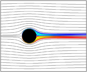
We consider the uniform two-dimensional incompressible flow of a viscous Newtonian fluid past a stationary, perfectly slipping circular cylinder of diameter $D$ and infinite span. A schematic of the set-up is shown in figure 1. The set-up is conveniently described in a polar coordinate system $(r,\theta )$, with $r$ and $\theta$ denoting the radial and circumferential coordinates, respectively. We consider steady flow, the governing equations for which are the stationary incompressible Navier–Stokes equations,

(2.1)\begin{equation} \rho( \boldsymbol{u}\boldsymbol{\cdot} \boldsymbol{\nabla} ) \boldsymbol{u} ={-}\boldsymbol{\nabla} p + \mu \nabla^2 \boldsymbol{u}, \quad \boldsymbol{\nabla} \boldsymbol{\cdot} \boldsymbol{u} = 0, \end{equation}

where $\boldsymbol {u}$ and $p$ denote the velocity and pressure fields, respectively, $\rho$ being the density and $\mu$, the dynamic viscosity of the fluid. The following no-through-flow and shear-free boundary conditions hold on the perfectly slipping cylinder's surface given by $r = a$ ($a = D/2$ being the radius of the circular cylinder):

(2.2a)\begin{gather} u_r(a,\theta) = 0, \end{gather}

(2.2b)\begin{gather}\tau_{r\theta}(a,\theta) = 0 \Leftrightarrow \left. \frac{\partial u_{\theta}}{\partial r}\right|_{r=a} = \frac{u_{\theta}(a,\theta)}{a}. \end{gather}

Here $u_r$ and $u_{\theta }$ denote the radial and circumferential components of the velocity vector $\boldsymbol {u}$. In (2.2b), $\tau _{r\theta }$ represents the $r\theta$ component of the viscous stress tensor $\boldsymbol {\tau } = \mu ( \boldsymbol {\nabla } \boldsymbol {u} + (\boldsymbol {\nabla } \boldsymbol {u})^T )$. Sufficiently far away from the cylinder, the flow attains a quiescent state corresponding to the uniform free stream along the positive $x$ direction. The far-field boundary conditions are given by

(2.3a–c)\begin{equation} u_r \to U_\infty \cos\theta, \quad u_\theta \to -U_\infty \sin\theta \quad \text{and} \quad p \to p_\infty \text{ as } r \to \infty, \end{equation}

where $U_\infty \boldsymbol {i}$ and $p_\infty$ denote the free-stream velocity and pressure, respectively, $\boldsymbol {i}$ being the unit vector in the $x$ direction. The flow is uniquely characterized by the Reynolds number $Re = \rho U_\infty D/ \mu$.

Figure 1. Schematic depicting the two-dimensional flow configuration consisting of a shear-free circular cylinder placed in a uniform crossflow of an incompressible Newtonian fluid. The coloured contours depict the vorticity field with the overlaid thin black lines representing the streamlines.

3. Asymptotic analysis

Potential flow theory provides a simple means of determining an approximation to the flow field. For the present set-up, the irrotational potential flow given by

(3.1a–c)\begin{equation} \bar{u}_r = U_\infty \left(1 \!-\! \frac{a^2}{r^2}\right) \cos\theta, \quad \bar{u}_\theta ={-}U_\infty \left(1 \!+\! \frac{a^2}{r^2}\right) \sin\theta, \quad \bar{p} = p_\infty \!+\! \frac{1}{2}\rho(U_\infty^2 \!-\! \bar{u}_r^2 - \bar{u}_\theta^2),\end{equation}

is a solution of not just the incompressible Euler's equations but also the incompressible Navier–Stokes equations (2.1). The term viscous potential flow is often employed in recognition of this important characteristic of the irrotational potential flow (Joseph, Funada & Wang Reference Joseph, Funada and Wang2007).

The potential flow solution satisfies the far-field conditions (2.3a–c) and the no-through-flow condition (2.2a). The corresponding tangential shear stress on the cylinder's surface is given by $\bar {\tau }_{r\theta }(a,\theta ) = (4 \mu U_\infty /a) \sin \theta$. Clearly, at any finite $Re$, the tangential shear stress over the cylinder surface predicted from the viscous potential flow solution does not vanish identically. The incompatibility between the potential flow solution and the shear-free boundary condition can also be viewed in terms of vorticity production at the shear-free interface. At the shear-free cylinder surface, a direct correspondence exists between the surface vorticity and the tangential surface velocity $\omega (a,\theta ) = 2 u_{\theta }(a,\theta )/a$, where $\omega$ denotes the vorticity component in the $z$ direction. Since $\bar {u}_{\theta }(a,\theta )$ is finite, the foregoing relationship would imply a contradictory existence of finite surface vorticity in an otherwise irrotational and inviscid flow field.

The apparent contradiction described above can be resolved by accounting for the existence of a boundary layer in the immediate vicinity of the shear-free cylinder surface. At high $Re$, this boundary layer, like its no-slip counterpart, is thin but significantly weaker as the relative change in the tangential surface velocity across it is $O(U_{\infty }Re^{-1/2})$ (as opposed to $O(U_{\infty })$ for a no-slip boundary). The vorticity produced in this thin boundary layer region is convected downstream first through a rear stagnation region and then eventually into a narrow wake. Modifications to the potential flow solution in each of these regions containing significant vorticity is necessary for elimination of an erroneous fore-aft symmetry in the irrotational flow field given by (3.1a–c). We note here that D'Alembert's paradox and the erroneous prediction of a zero-net-momentum-deficit wake are both direct consequences of the fore-aft symmetry of the potential flow solution. In the forthcoming subsections we develop interdependent asymptotic analyses necessary to account for the finite vorticity production, and its advection and diffusion into each of the distinct subregions (boundary layer, stagnation zone and wake) of the flow field.

3.1. Boundary layer analysis

At sufficiently high Reynolds numbers ($Re \gg 1$), the corrections to the potential flow solution that are necessary to enforce the shear-free condition (2.2b) can be sought within the broad purview of boundary layer theory. To analyse the flow characteristics in the boundary layer region, we define a scaled normal coordinate $y=(r-a)/a$ that is attached to the cylinder surface, along with a new tangential coordinate $\phi = {\rm \pi}- \theta$. The origin of the ($y,\phi$) coordinate system coincides with the forward stagnation point. In this newly defined $(y,\phi )$ coordinate system, we next express the flow variables as a superposition of the potential flow solution and a correction over it, i.e.

(3.2a–c)\begin{equation} u_y = \bar{u}_y + \tilde{u}_y, \quad u_\phi = \bar{u}_\phi + \tilde{u}_\phi, \quad p = \bar{p} + \tilde{p}, \end{equation}

where $\bar {u}_y$ and $\bar {u}_\phi$ are the normal and tangential potential flow velocity components in the $(y, \phi )$ coordinate system while $\bar {p}$ denotes the pressure deduced from the potential flow theory. The corresponding corrections to the velocity components and the pressure field are denoted by $\tilde {u}_y$, $\tilde {u}_\phi$ and $\tilde {p}$, respectively. Using (3.2b) and (3.1b) in (2.2b), we arrive at the following expression for the shear-free condition at the surface of the cylinder $y=0$,

(3.3)\begin{equation} \left.\frac{\partial \tilde{u}_{\phi}}{\partial y}\right|_{y = 0} = 4U_\infty\sin\phi + \tilde{u}_{\phi}|_{y = 0}. \end{equation}

Inside the boundary layer region, the thickness of the boundary layer serves as an appropriate length scale along the normal direction. Denoting the boundary layer thickness scaled with $a$ by $\delta$, we find that within the boundary layer $(\partial /\partial y) \sim 1/\delta$. The potential flow velocity components $\bar {u}_\phi$ and $\bar {u}_y$ in the boundary layer scale as $U_{\infty }$ and $U_{\infty }\delta$, respectively. Using the above facts and (3.3), we deduce that in the boundary layer $\tilde {u}_\phi \sim U_{\infty }\delta$. The divergence-free constraint on the velocity field yields $\tilde {u}_y \sim U_{\infty }\delta ^2$. To arrive at the boundary layer equations, we define a stretched coordinate system $(y^\ast , \phi )$ with a normalization in the normal direction: $y^\ast = y/\delta$. Furthermore, we define the following non-dimensional velocity components

(3.4a,b)\begin{equation} u_\phi^\ast{=} \frac{u_\phi}{U_\infty}, \quad u_y^\ast{=} \frac{u_y}{U_\infty\delta}. \end{equation}

In the stretched coordinate system $(y^\ast , \phi )$, the circumferential momentum equation assumes the following form:

(3.5)\begin{align} &u_y^\ast\frac{\partial u_\phi^\ast}{\partial y^\ast} + \frac{u_\phi^\ast}{(y^\ast \delta + 1)} \frac{\partial u_\phi^\ast}{\partial \phi} + \frac{\delta u_y^\ast u_\phi^\ast}{(y^\ast\delta+1)}={-}\frac{1}{(y^\ast \delta + 1)\rho U_\infty^2}\frac{\partial p}{\partial \phi} + \frac{\mu}{\rho U_\infty a \delta^2} \nonumber\\ &\quad \times \left(\frac{\partial^2 u_\phi^\ast}{\partial y^{{\ast} 2}} + \frac{\delta}{(y^\ast\delta + 1)}\frac{\partial u_\phi^\ast}{\partial y^\ast}- \frac{\delta^2 u_\phi^\ast}{(y^\ast \delta + 1)^2}+ \frac{\delta^2}{(y^\ast \delta + 1)^2}\frac{\partial^2 u_\phi^\ast}{\partial \phi^{2}} + \frac{2 \delta^3}{(y^\ast \delta + 1)^2}\frac{\partial u_y^\ast}{\partial \phi}\right). \end{align}

The convective and the diffusive terms are both dominant in the boundary layer and, hence, the quantity $\mu /(\rho U_\infty a \delta ^2) = 2/(Re\delta ^2)$ should be $O(1)$. Without loss of generality, we set $\delta = \sqrt {2/Re}$.

In the boundary layer coordinates $(y^\ast , \phi )$, the radial momentum equation assumes the following non-dimensional form:

(3.6)\begin{align} &\delta^2 u_y^\ast\frac{\partial u_y^\ast}{\partial y^\ast} + \frac{\delta^2 u_\phi^\ast}{(y^\ast \delta + 1)}\frac{\partial u_y^\ast}{\partial \phi} - \underline{\frac{\delta u_\phi^{{\ast} 2}}{(y^\ast\delta+1)}} ={-} \underline{ \frac{1}{\rho U_\infty^2}\frac{\partial p}{\partial y^\ast} } \nonumber\\ &\quad +\delta^2\left(\frac{\partial^2 u_y^\ast}{\partial y^{{\ast} 2}} + \frac{\delta}{(y^\ast \delta +1)}\frac{\partial u_y^\ast}{\partial y^\ast} - \frac{\delta^2 u_y^\ast}{(y^\ast \delta +1)^2} + \frac{\delta^2}{(y^\ast \delta +1)^2} \frac{\partial^2 u_y^\ast}{\partial \phi^2} - \frac{2 \delta}{(y^\ast \delta +1)^2}\frac{\partial u_\phi^\ast}{\partial \phi} \right). \end{align}

From the above relationship, one can deduce that in the boundary layer region, the contribution to the pressure from the inviscid potential flow $\bar {p}$ provides the centripetal force necessary for the flow to turn around the cylinder (signified through the underlined terms in the foregoing relationship (3.6)). The pressure perturbation $\tilde {p}$ therefore scales as $O(\delta ^2)$.

Next, we invoke boundary layer approximations and retain only the most significant terms. Using (3.2a–c) in (3.5) along with the potential flow variables (3.1a–c), to a leading order, we obtain the following for the non-dimensional correction velocity component along the circumferential direction $\tilde {u}_\phi ^\ast = \tilde {u}_\phi /(U_\infty \delta )$:

(3.7)\begin{equation} \frac{\partial^2 \tilde{u}_\phi^\ast}{\partial y^{{\ast} 2}} ={-}2 y^\ast \cos\phi \frac{\partial \tilde{u}_\phi^\ast}{\partial y^\ast} + 2\sin\phi \frac{\partial \tilde{u}_\phi^\ast}{\partial\phi} + 2\tilde{u}_\phi^\ast \cos\phi. \end{equation}

With only the leading-order terms retained, the boundary conditions (2.2b) and (2.3a–c) reduce to

(3.8a–c)\begin{equation} \tilde{u}_\phi^\ast{=} 0 \text{ at } \phi = 0, \quad \tilde{u}_\phi^\ast \rightarrow 0\quad \text{ as } y^\ast \rightarrow\infty, \quad \frac{\partial\tilde{u}_\phi^\ast}{\partial y^\ast} = 4\sin\phi \text{ at } y^\ast{=} 0. \end{equation}

Note that the condition (3.8a) follows from the symmetry of the flow.

Boundary layer equations do not posses a characteristic scale and admit a dimension reduction through a similarity transformation. In typical planar and axisymmetric flows, the reduction in dimension facilitates simplification of the original partial differential equation and the associated boundary conditions into an ordinary differential equation and corresponding boundary conditions. A similarity transformation was also employed by Moore (Reference Moore1963) in his analysis of an axisymmetric boundary layer formed over a shear-free sphere. Given its wide-ranging success in a variety of flows lacking an inherent characteristic scale, it is natural to seek a similarity solution of the boundary layer equation for our present cylindrical set-up.

An analysis of the boundary layer equation (3.7) allows us to establish that a dimensional reduction of (3.7) is indeed possible, albeit for a slightly modified form of boundary condition (3.8c). Specifically, we show existence of a family of similarity solutions

(3.9)\begin{equation} \tilde{u}_{\phi, n}^\ast{=}{-}\frac{\left(\sin\dfrac{\phi}{2}\right)^{2n+2}}{\sqrt{{\rm \pi} }\sin\phi}\int_0^{{\rm \pi} } \exp\left(\frac{-\eta^2}{2\cos^2\left(\dfrac{\alpha}{2}\right)}\right) \sin^{2n+2}\left(\frac{\alpha}{2}\right)\,\mbox{d}\alpha, \end{equation}

where $\eta =\sqrt 2 y^\ast \cos ({\phi }/{2})$ and $n = 0,1,2,\ldots$ is a non-negative integer (see Appendix A for details). Each $\tilde {u}_{\phi , n}^\ast$ satisfies (3.7), (3.8a,b) and the boundary condition

(3.10)\begin{equation} \frac{\partial\tilde{u}_{\phi, n}^\ast}{\partial y^\ast}=f_n(\phi) = \left[\sin\left(\frac{\phi}{2}\right)\right]^{2n+1} \mbox{ at } y^\ast{=}0. \end{equation}

Unfortunately, none of these unique solutions $\tilde {u}_{\phi , n}^\ast$ can individually be made to satisfy the boundary condition (3.8c). This is in striking contrast to the case of flow past a shear-free sphere wherein a single similarity transformation can be used to reduce the parabolic boundary layer equation and determine its closed-form solution (Moore Reference Moore1963; Leal Reference Leal2007).

The hindrance posed by the incompatibility between the derived similarity solutions and the boundary condition (3.8c) can be overcome by exploiting the linearity of the governing equation (3.7). Next, as shown in Appendix A, using the relationship

(3.11)\begin{equation} 4\sin \phi = \sum_{n=0}^\infty w_n \left(\sin\frac{\phi}{2}\right)^{2n+1}, \quad \mbox{where } w_0 = 8 \mbox{ and } w_n = 8\prod_{i=1}^n \frac{(2i-3)}{2i} \mbox{ for } n > 0, \end{equation}

the final solution to (3.7) and (3.8a–c) can be expressed as an infinite superposition of self-similar terms ($\tilde {u}_\phi ^\ast = \sum _{n=0}^\infty w_n \tilde {u}_{\phi , n}^\ast$) as follows:

(3.12)\begin{equation} \tilde{u}_\phi^\ast{=} \frac{-4}{\sqrt{{\rm \pi} }}\tan\left(\frac{\phi}{2}\right) \int_0^{{\rm \pi} } \exp\left(\frac{-\eta^2}{2\cos^2 \left(\dfrac{\alpha}{2}\right)}\right)\sin^2\left(\frac{\alpha}{2}\right) \sqrt{1 - \sin^2\left(\frac{\alpha}{2}\right)\sin^2\left(\frac{\phi}{2}\right)} \,\mbox{d}\alpha. \end{equation}

The above solution is in the form of superposition of infinitely many self-similar terms as opposed to the more commonly encountered solution consisting of a single self-similar term (as in the case of a shear-free sphere Moore Reference Moore1963).

Vorticity produced at the shear-free cylinder's surface is convected and diffused throughout the boundary layer region. An estimate of this vorticity $\omega _{bl}$ can be obtained from the solution (3.12) as follows:

(3.13)\begin{align} \omega_{bl}^\ast &= \frac{\omega_{bl}}{(U_\infty / a)} = \frac{a}{U_\infty}\left(\frac{\partial u_\theta}{\partial r}+ \frac{u_\theta}{r}-\frac{1}{r}\frac{\partial u_r}{\partial \theta} \right) ={-}\frac{\partial \tilde{u}_\phi^\ast}{\partial y^\ast} + O(\delta) \nonumber\\ & \approx{-}\sqrt{\frac{32}{{\rm \pi} }} \sin\left( \frac{\phi}{2} \right) \int_0^{{\rm \pi} } \eta \exp \left(\frac{-\eta^2}{2\cos^2\left(\dfrac{\alpha}{2}\right)}\right) \tan^2\left(\frac{\alpha}{2}\right) \sqrt{1 - \sin^2\left( \frac{\alpha}{2} \right) \sin^2\left( \frac{\phi}{2} \right)} \, \mbox{d}\alpha. \end{align}

Here the superscript ‘$^\ast$’ is used to denote non-dimensional vorticity.

3.2. Rear stagnation region analysis

The boundary layer analysis (BLA) of the previous subsection was based on the assumption of wall-normal gradients being significantly larger than the streamwise gradients. The surface-normal flow gradients diminish progressively with a gradual increase in the thickness of the boundary layer along the periphery of the cylinder. In the vicinity of the rear stagnation point ($(y,\phi ) = (0,{\rm \pi} )$), as the flow undergoes a sharp turn, the reduction in flow gradients in the surface-normal direction is so significant that they become comparable to those in the circumferential direction. Thus, in the neighbourhood of the rear stagnation point, the boundary layer assumptions do not hold and, hence, the analysis of the previous section becomes unreliable. To complete the description of the flow over the entire shear-free cylinder boundary, we next analyse the flow in the vicinity of the rear stagnation region without invoking boundary layer assumptions.

The flow in the neighbourhood of the rear stagnation region involves a viscous boundary layer that effuses out into an inviscid flow (see figure 1 and the forthcoming analysis). This specific flow scenario corresponds closely to the one concerned with flow near a stagnation point on a rigid boundary (Harper Reference Harper1963). In particular, close to the rear stagnation point we expect dominance of the convective terms over the diffusive terms and an appreciable variation in vorticity but not the velocity. To analyse the flow in the stagnation region, we adopt the $(y, \theta )$ coordinates ($y$ as defined in § 3.1) so that the origin of the coordinate system coincides with the rear stagnation point. Our analysis closely follows the work of Harper (Reference Harper1963), in particular, (18) on page 148 of this cited work. Specifically, a scaling analysis of the most significant terms allows identification of two distinct regions with contrasting scenarios. The first region in which the convective terms dominate the viscous terms is centred around the rear stagnation point and extends to a distance of $O(1)$ into the boundary layer. The boundary layer assumptions themselves however are valid only beyond a certain distance from the rear stagnation point. This distance scales with the Reynolds number as $O(Re^{-1/4})$. Therefore, there exists a region of dimension $O(Re^{-1/4}) \ll \theta \ll O(1)$ over which the boundary layer assumptions are valid and the flow itself is inviscid.

We next develop a theoretical model for analysis of flow in the neighbourhood of the rear stagnation region. As shown below, the analysis independently provides justification for the aforementioned scaling arguments. In the vicinity of the stagnation region, i.e. towards the final stage of the boundary layer, vorticity is given by

(3.14)\begin{equation} \lim_{\phi \to {\rm \pi}} \omega_{bl}^\ast{=}{-}\sqrt{\frac{32}{{\rm \pi} }}\int_0^{{\rm \pi} } \eta \exp\left(\frac{-\eta^2}{2\cos^2\left(\dfrac{\alpha}{2}\right)}\right) \frac{\sin^2\left(\dfrac{\alpha}{2}\right)}{\cos\left(\dfrac{\alpha}{2}\right)}\,\mbox{d}\alpha, \quad \text{where } \eta = \frac{y\theta}{\sqrt{2}\delta}. \end{equation}

In this final stage of the boundary layer, the velocity variations are small. Consequently, in an overlap region within which the solutions from the BLA and the stagnation region analysis are both valid and should match, the distortion in the streamfunction $\tilde {\psi }$ is negligible compared with the contribution to the streamfunction from the potential flow $\bar {\psi }$. This region is off-axis and is located away from the singular rear stagnation point at $\theta =0$. In this region, the net streamfunction $\psi$ which is the sum of the above two, assumes the asymptotic form $\psi = \bar {\psi } + \tilde {\psi } \approx \bar {\psi } \approx 2 U_\infty a y \theta$ ($\bar {\psi } = U_{\infty }ay(2+y)\sin \theta /(1+y) = 2U_{\infty }ay\theta$ for $y \ll 1$ and $\theta \ll 1$). Using this asymptotic form, $\eta$ can be rewritten as

(3.15)\begin{equation} \eta = \frac{\psi}{2 \sqrt{2} U_\infty a \delta} = \frac{\psi_s^\ast}{2 \sqrt{2}}, \end{equation}

where $\psi _s^\ast = \psi / (U_\infty a \delta )$ is the non-dimensional streamfunction near the rear stagnation point. Combining expressions (3.15) and (3.14) we obtain an expression for vorticity in the final stage of the boundary layer. Since the rear stagnation region is governed by inviscid dynamics, vorticity remains constant along streamlines. We therefore arrive at the following expression for vorticity in the stagnation region:

(3.16)\begin{equation} \omega_s^\ast{=}{-}\frac{2}{\sqrt{{\rm \pi} }}\int_0^{{\rm \pi} } \psi_s^\ast \exp\left(\frac{-\psi_s^{{\ast} 2}}{16 \cos^2\left(\dfrac{\alpha}{2}\right)}\right)\frac{\sin^2\left(\dfrac{\alpha}{2}\right)} {\cos\left(\dfrac{\alpha}{2}\right)}\,\mbox{d}\alpha. \end{equation}

Here $\omega _s^\ast$ is the non-dimensional vorticity in the stagnation region ($\omega _s^\ast = \omega _s a / U_\infty$).

The resultant vorticity from the end of the boundary layer region is simply transported along the streamlines into the rear stagnation region. In the overlap region the distortion in the streamfunction $\tilde {\psi } = O(Re^{-1})$ is insignificant since the potential flow streamfunction $\bar {\psi } = O(Re^{-1/2})$. The potential flow streamfunction $\bar {\psi }$ remains $O(Re^{-1/2})$ in the stagnation region. Next, consider a potential flow streamline that is located $O(\delta )$ distance away from the cylinder's surface in the boundary layer region. In the rear stagnation region this streamline moves to $O(\delta ^{1/2})$ distance from the cylinder's surface and maintains the $O(\delta ^{1/2})$ distance from the line of symmetry near the stagnation point. The flow at the rear stagnation point corresponds closely to the flow in a right-angled corner. For such a stagnation point flow, both the directions $y$ and $\theta$ must be equally important or, in other words, $y \sim \theta$. Furthermore, the flow itself must turn around the corner so that $\psi \sim y \theta$. Next, noting that vorticity is produced solely from the distortion in the streamfunction, we deduce that $\tilde {\psi } \sim O(Re^{-1/2})$ in the rear stagnation region. Moreover, $y, \theta \sim \delta ^{1/2}$ or, equivalently, the size of the stagnation region is $O(Re^{-1/4})$, in accordance with our assertion in the preceding paragraphs.

In view of the above arguments, to analyse the rear stagnation point flow, we next introduce an appropriately rescaled coordinate system $(y_s^\ast , \theta _s^\ast )$, where $y_s^\ast = y/\delta ^{1/2}$ and $\theta _s^\ast = \theta /\delta ^{1/2}$. In our present planar set-up, an absence of vortex stretching mechanisms suggests that the vorticity level in the stagnation zone matches that in the boundary layer region. Thus, $\omega _s^\ast \sim O(1)$, which can be inferred from (3.16) as well. For a non-dimensional vorticity that scales as $O(1)$, the associated non-dimensional velocity corrections to the inviscid flow must necessarily scale as the characteristic non-dimensional length scale, or equivalently $O(Re^{-1/4})$.

An inspection of the expression (3.1a,b) reveals that in the rear stagnation region, the potential velocity components themselves scale as $O(Re^{-1/4})$. This would imply that both the correction and the potential flow components exhibit similar scalings and are therefore comparable in magnitude. Expressing vorticity as the curl of the velocity vector and retaining only the significant terms as determined from the appropriate scales in the rear stagnation region, we deduce that

(3.17)\begin{equation} \frac{\partial \tilde{u}_{\theta_{(s)}}^\ast}{\partial y_s^\ast}- \frac{\partial \tilde{u}_{y_{(s)}}^\ast}{\partial \theta_s^\ast} = \omega_s^\ast, \end{equation}

where $\tilde {u}_{\theta _{(s)}}^\ast = \tilde {u}_\theta / ( U_\infty \delta ^{1/2})$ and $\tilde {u}_{y_{(s)}}^\ast = \tilde {u}_r /( U_\infty \delta ^{1/2} )$ are the non-dimensional correction velocity components in the circumferential and radial directions, respectively. The correction velocity components can be expressed in terms of the distortion to the streamfunction as follows:

(3.18a,b)\begin{equation} \tilde{u}_{y_{(s)}}^\ast{=} \frac{\partial \tilde{\psi}_s^\ast}{\partial \theta_s^\ast},\quad \tilde{u}_{\theta_{(s)}}^\ast{=}{-}\frac{\partial \tilde{\psi}_s^\ast}{\partial y_s^\ast}. \end{equation}

Using (3.16) and (3.18a,b) in the relationship (3.17), we obtain the following governing equation for the correction velocity induced distortion in the streamfunction:

(3.19)\begin{equation} \frac{\partial^2 \tilde{\psi}_s^\ast}{\partial y_s^{{\ast} 2}} + \frac{\partial^2 \tilde{\psi}_s^\ast}{\partial \theta_s^{{\ast} 2}} ={-}\omega_s^\ast{=} \frac{2}{\sqrt{{\rm \pi} }}\int_0^{{\rm \pi} } (\tilde{\psi}_s^\ast{+} \bar{\psi}_s^\ast) \exp\left(\frac{-(\tilde{\psi}_s^\ast{+} \bar{\psi}_s^\ast)^2}{16 \cos^2\left(\dfrac{\alpha}{2}\right)}\right) \frac{\sin^2\left(\dfrac{\alpha}{2}\right)}{\cos\left(\dfrac{\alpha}{2}\right)}\,\mbox{d}\alpha. \end{equation}

Here $\tilde {\psi }_s^\ast = \tilde {\psi } / ( U_\infty a \delta )$ and $\bar {\psi }_s^\ast = \bar {\psi } /( U_\infty a \delta ) = 2 y_s^\ast \theta _s^\ast$ are the non-dimensional distortion and potential flow streamfunctions in the rear stagnation region, respectively. The correction flow becomes unidirectional in the final stage of the boundary layer and towards the beginning of the wake. These facts combined with the no-through-flow condition at the cylinder surface and the symmetry condition along the rear axis of symmetry ($\theta = 0$), give rise to the following boundary conditions on the distortion streamfunction $\tilde {\psi }_s^\ast$:

(3.20a–c) \begin{equation} \tilde{\psi}_s^\ast{=} 0 \text{ at } y_s^\ast, \theta_s^\ast{=}0 , \quad \frac{\partial \tilde{\psi}_s^\ast}{\partial y_s^\ast} \rightarrow 0\quad \text{ as } y_s^\ast\rightarrow\infty, \quad \frac{\partial \tilde{\psi}_s^\ast}{\partial \theta_s^\ast} \rightarrow 0\quad \text{ as } \theta_s^\ast\rightarrow\infty. \end{equation}

We note here that owing to the relationship (3.16), the above homogeneous boundary condition on the distortion streamfunction enforces the shear-free condition as well (to a leading order, the homogeneous boundary condition for surface vorticity and the shear-free constraint at the cylinder's boundary are equivalent).

Equation (3.19) is an elliptic partial integro-differential equation that involves a non-local source term. The nonlinearity of (3.19) makes its analytical tractability extremely challenging, if not impossible. This complication arises principally because the perturbations to the potential flow turn out to be comparable to the flow itself in the rear stagnation region. A similar nonlinearity was encountered in the planar analysis of two-dimensional stagnation point flow (Harper Reference Harper1963). We note here that in an axisymmetric configuration, a reduction in the magnitude of vorticity due to contraction of vortex lines in the stagnation region ensures that perturbations remain insignificant in comparison with the base potential flow (Harper & Moore Reference Harper and Moore1968). This insignificance of the perturbations facilitates full analytical resolution of the axisymmetric flow in the vicinity of the rear stagnation region of a shear-free spherical surface (Moore Reference Moore1963).

To make further progress, we solve (3.19) subject to boundary conditions (3.20a–c) numerically using standard approximation techniques. Note that the vorticity field from the boundary layer solution (3.13) is regular and bounded ($|\omega ^\ast _{bl}| \leq 4$) and, hence, the right-hand side of (3.19) and the corresponding integral solution are both regular. This regularity enables discretization of (3.19) using standard approximation techniques. Our numerical implementation is detailed in Appendix B. Our analysis of the rear stagnation and the boundary layer regions provides a complete description of the flow along the periphery and in the immediate neighbourhood of the shear-free cylinder. Figure 2 depicts the scaled tangential velocity correction $\tilde {u}_\phi ^{\ast } = \sqrt {Re / 2} (\tilde {u}_\phi /U_{\infty })$ along the surface of the cylinder predicted from our analysis of the present and preceding subsections at $Re = 10^2$, $10^3$, $10^4$ and $10^5$. Coloured solid lines in figure 2 illustrate the trends for the rear stagnation region obtained from the numerical solution of (3.19) and (3.20a–c). The numerical solution is only valid in the neighbourhood of the rear stagnation point. Hence, the coloured solid lines extend only over a limited range of $\phi$ representing a portion of the rearward cylinder surface. The scaled tangential velocity correction increases in magnitude and subsequently decreases after attaining a maxima as one traverses from the rear stagnation point to the forward stagnation point along the cylinder surface. This broad trend is observed at all the four Reynolds numbers, with both the magnitude of the peak and the spread in $\tilde {u}_\phi ^{\ast }$ strongly dependent on the Reynolds number. We note here that this apparent dependence on $Re$ is entirely due to the disparity between normalization scales employed in figure 2 and the relevant characteristic scales in the stagnation region ($\delta$ vs $\sqrt {\delta }$ for the velocity scale for instance).

Figure 2. The scaled correction in the tangential surface velocity ($\tilde {u}_\phi ^{\ast } = \sqrt {Re / 2} (u_\phi - \bar {u}_\phi )/U_{\infty }$) along the shear-free cylinder surface at Reynolds numbers $10^2$, $10^3$, $10^4$ and $10^5$. Predictions from the boundary layer analysis (BLA) and the rear stagnation region analysis (RSRA) are indicated using solid black and solid coloured lines, respectively. Dotted coloured lines represent results from direct numerical simulations (DNS).

Solid black lines in figure 2 depict the scaled tangential velocity correction deduced from the BLA (i.e. from (3.12)). Owing to the boundary layer specific characteristic scale based normalization employed in figure 2, $\tilde {u}_\phi ^{\ast }$ given by (3.12) is independent of the Reynolds number and so are the solid black lines depicted in each of the four frames of figure 2. The scaled correction $\tilde {u}_\phi ^{\ast }$ grows monotonically with $\phi$. The growth is particularly pronounced over the rearward cylinder surface ($\phi \geq {\rm \pi}/2$). In particular, $\tilde {u}_\phi ^{\ast }$ becomes unbounded in the vicinity of the rear stagnation point. This unphysical divergence of $\tilde {u}_\phi ^{\ast }$ as $\phi \rightarrow {\rm \pi}$ is a direct consequence of the breakdown of the assumptions inherent in the BLA.

To determine $\tilde {u}_\phi ^{\ast }$ over the entire cylinder periphery, we must employ complementary boundary layer and stagnation region analyses over their respective domains of validity. Furthermore, a matching procedure must be invoked over the overlap region $O(Re^{-1/4}) \ll \theta \ll O(1)$ to obtain a uniformly valid solution $\tilde {u}_\phi ^{\ast }$ over the entire range $0 \leq \phi \leq {\rm \pi}$. The dependence of $\tilde {u}_\phi ^{\ast }$ on $\phi$, as illustrated in figure 2, suggests that such a matching is indeed possible, albeit at sufficiently high $Re$, which is when our asymptotic analyses of boundary layer and stagnation regions are strictly valid (i.e. in the limit $Re \rightarrow \infty$).

Our theoretical results can be directly compared with the predictions from detailed simulations. To this end, we perform direct numerical simulations (DNS) of a two-dimensional unsteady incompressible flow past a shear-free circular cylinder using a well-established technique in polar cylindrical coordinates (see Shukla & Zhong (Reference Shukla and Zhong2005) and Shukla, Tatineni & Zhong (Reference Shukla, Tatineni and Zhong2007) for details and verification tests). In brief, our simulation methodology relies on a combination of tenth-order compact finite difference and Fourier-spectral schemes (in $r$ and $\theta$ coordinates, respectively) and a second-order semi-implicit projection scheme (Hugues & Randriamampianina Reference Hugues and Randriamampianina1998) for spatiotemporal discretization. In all our runs we employ spatiotemporal resolutions necessary to resolve the thin boundary layers and enforce the Courant–Friedrichs–Lewy convective stability criterion. We also perform long-time simulations on successively refined meshes to ensure mesh independence of the computed solution.

The predictions from our DNS runs are depicted in figure 2 alongside results from the asymptotic BLA and the rear stagnation region analysis (RSRA). The comparison is quite encouraging and more so at high Reynolds numbers. Specifically, over the windward section of the cylinder's boundary, discernible deviations between the DNS results and BLA are evidenced at $Re = 10^2$. The deviations reduce progressively with an increase in the Reynolds number. In particular, at the highest $Re = 10^5$, the predictions from BLA agree remarkably well with the DNS results all the way up to the location at which a maximum in the magnitude of $\tilde {u}_\phi ^{\ast }$ is encountered. We observe trends similar to those noted for the BLA in the rear stagnation region as well. Appreciable deviations are evidenced between the predictions from RSRA and the DNS results at Reynolds numbers of $10^2$ and $10^3$. The deviations reduce considerably at $Re = 10^4$ and are only marginal at the highest Reynolds number of $Re = 10^5$ investigated in our work. Overall, at a given $Re$, the discrepancy between DNS and RSRA is discernibly more pronounced than the discrepancy between DNS and BLA. This increased discrepancy is attributable to the more stringent restrictions on the Reynolds numbers that are necessary in RSRA ($Re^{-1/2} \ll 1$ for the BLA vs $Re^{-1/4} \ll 1$ in the case of RSRA).

We note here that viscous terms do become important in the immediate vicinity of the rear stagnation point. The presence of such a viscous sublayer region in general stagnation point flows was mentioned in Harper (Reference Harper1963). The scale of this relatively thin region is $O(Re^{-3/4})$, a fact that can be readily established by appealing to the vorticity transport equation with consideration of viscous diffusion. The scale of this region implies that its contribution to the leading-order terms of interest in this work is insignificant.

3.3. Analysis of the wake region

To complete our description of the vortical regions of the flow field, we next develop an asymptotic analysis of the narrow downstream wake region into which the vorticity generated at the shear-free cylindrical surface is eventually convected (see figure 1). We adopt a Cartesian coordinate system $(x,z)$ where both the scaled coordinates $x$ and $z$ are normalized with respect to the cylinder's radius $a$. The origin of the coordinate system coincides with the rear stagnation point with the $x$-axis pointing along the streamwise direction.

As argued in the earlier subsection, an absence of a vortex stretching mechanism in the present planar configuration implies that the non-dimensional vorticity ($\omega ^{\ast } = a\omega /U_{\infty }$) scales as $O(1)$ in the boundary layer and stagnation regions, and crucially, in the initial stages of the wake region as well. The wake thickness is the appropriate length scale for characterization of the wake region. Denoting the wake thickness normalized with the cylinder radius by $\delta _w$ and making use of the non-dimensional vorticity scale of $O(1)$, we deduce that the correction velocity in the streamwise direction $\tilde {u}_x$ should scale as $O(\delta _w)$. Applying the divergence-free condition on the correction velocity field, we obtain $\tilde {u}_z \sim O(\delta _w^2)$ as the characteristic scale for the component of the correction velocity in the $z$ direction.

In the wake region the inviscid base flow velocity components deduced from the potential flow theory can be shown to scale as $\bar {u}_x \sim O(1)$ and $\bar {u}_z \sim O(\delta _w)$, respectively. Balancing out the convective and the diffusive terms in the wake, in a way similar to our analysis of the boundary layer region, we obtain $\delta _w \sim \delta$. Without loss of generality, we set $\delta _w = \delta$. Using the characteristic scales described above, we next define appropriately normalized spatial coordinates and the base potential flow and correction velocity components as follows:

(3.21a–e)\begin{equation} z^\ast{=} \frac{z}{\delta},\quad \bar{u}_x^\ast{=} \frac{\bar{u}_x}{U_\infty},\quad \bar{u}_z^\ast{=} \frac{\bar{u}_z}{U_\infty\delta},\quad \tilde{u}_x^\ast{=} \frac{\tilde{u}_x}{U_\infty\delta},\quad \tilde{u}_z^\ast{=} \frac{\tilde{u}_z}{U_\infty\delta^2}.\end{equation}

With the above definitions in place, the equation that governs the distribution of non-dimensional vorticity $\omega _w^\ast = \omega _w a/U_\infty$ in the wake region assumes the following linearized form:

(3.22)\begin{equation} \bar{u}_{x_0}^\ast \frac{\partial \omega_w^\ast}{\partial x} + \bar{u}_{z_0}^\ast \frac{\partial \omega_w^\ast}{\partial z^\ast} = \frac{\partial^2 \omega_w^\ast}{\partial z^{{\ast} 2}}. \end{equation}

Here we have only retained the leading-order terms, and, $\bar {u}_{x_0}^\ast$ and $\bar {u}_{z_0}^\ast$ denote the zeroth-order terms in an expansion of $\bar {u}_x^\ast$ and $\bar {u}_z^\ast$ about $z^\ast = 0$, respectively. Imposition of symmetry of the flow field about $z^\ast = 0$ and the irrotationality of the far-field flow leads to the boundary conditions

(3.23a,b)\begin{equation} \omega_w^\ast{=} 0 \text{ at } z^\ast{=} 0, \quad\omega_w^\ast\to 0 \text{ as }z^\ast\to\infty.\end{equation}

Moreover, we require the solution $\omega _w^\ast$ of (3.22) subject to boundary conditions (3.23a,b) to be such that it results in a drag-producing far wake with a constant momentum deficit. The general solution of (3.22) and (3.23a,b) that satisfies the aforementioned criterion assumes the form

(3.24)\begin{equation} \omega_w^\ast{=} \sum_{n} \frac{ \lambda_n \zeta_n \exp\left( -\dfrac{\zeta_n^2}{2}\right)}{ \left( x+ 1 + \dfrac{1}{x+ 1} + c_n\right)}, \quad \text{where } \zeta_n=\frac{z^\ast \left(1 - \dfrac{1}{(x+ 1)^2}\right)} {\sqrt{2}\left(x+1+\dfrac{1}{x+1}+c_n\right)^{1/2}}. \end{equation}

Like the solution (3.12) of the boundary layer (3.7), the above solution is in the form of superposition of a family of infinite self-similar wake solutions each with strength $\lambda _n$ and centred around the coordinates $(-(c_n+1),0)$. We require the yet to be determined constants $\lambda _n$ and $c_n$ in the above expression (3.24) to be such that the asymptotic forms of $\omega _w^\ast$ and $\omega _{bl}^\ast$ match in the rear stagnation region. Note that since the flow in the rear stagnation region is symmetric in $y$ and $\theta$, the vorticity in the beginning of the wake region must match the one associated with the final stage of the boundary layer. The transition of the flow from the stagnation region to the wake region is thus, to leading order, an inversion of the flow coming from the boundary layer into the stagnation region. Therefore, the distortion in the streamfunction becomes smaller at the right side of the stagnation region (beginning of the wake region). Consequently, the vorticity in the beginning of the wake region is of a form given by the expression (3.14). Matching the general solution of the vorticity in the wake region given by (3.24) and the vorticity distribution given by (3.14) allows us to determine the final form of $\omega _w^\ast$,

(3.25)\begin{equation} \omega_w^\ast{=}{-}\sqrt{\frac{2}{{\rm \pi} }} \int_{{-}2}^{2} \frac{ \zeta_\kappa \exp\left( -\dfrac{\zeta_\kappa^2}{2}\right) \sqrt{4 - \kappa^2} }{ \left( x+ 1 + \dfrac{1}{x+ 1} - \kappa\right)} \, \textrm{d}\kappa, \quad \text{where } \zeta_\kappa= \frac{z^\ast \left(1 - \dfrac{1}{(x+ 1)^2}\right)}{\sqrt{2}\left(x\!+\!1\!+\!\dfrac{1}{x+1} - \kappa\right)^{1/2}}. \end{equation}

At a location far downstream, i.e. when $x \gg 1$, (3.25) assumes the asymptotic form

(3.26)\begin{equation} \omega_w^\ast \rightarrow -\frac{2 \sqrt{{\rm \pi} }z^\ast}{x^{ 3/2}}\exp\left( -\frac{z^{{\ast} 2}}{4 x} \right) \quad \mbox{for } x \rightarrow \infty. \end{equation}

The above asymptotic expression is precisely in the form of the well-known self-similar solution for the defect velocity in the laminar wake of a planar body with a given drag coefficient (Schlichting & Gersten Reference Schlichting and Gersten2003). A comparison with the solution for the defect velocity from Schlichting & Gersten (Reference Schlichting and Gersten2003) reveals that sufficiently far away from the cylinder surface, the wake solution (3.25) exhibits an asymptotic decay rate that corresponds to a drag coefficient of $16{\rm \pi} /Re$. As shown in the forthcoming section, to a leading order, the drag coefficient associated with the flow past a shear-free circular cylinder matches the aforementioned value of $16{\rm \pi} /Re$ exactly. Thus, our combined asymptotic analysis of the boundary layer, rear stagnation and the wake regions is self-consistent in that the drag predicted from the analysis, as derived in the forthcoming section, equals the one deduced from the far-field wake signature.

4. Viscous dissipation and drag coefficient

The viscous corrections to the inviscid base state induce a streamwise asymmetry in the otherwise symmetric stress field. The viscous correction-induced circumferential asymmetry in the surface stress gives rise to a non-vanishing drag force. We next attempt to quantify the finite drag force and in the process resolve D'Alembert's paradox specifically for the configuration being investigated.

An expression for the net drag force can be derived by summing up the componentwise contributions from the pressure and viscous stresses along the $x$ direction. Given the asymptotic form of the solution, such an expression would be tantamount to summing up the contributions from the zeroth-order inviscid base flow and the first-order viscous correction to it. Owing to the symmetry of the inviscid base flow, the contributions to the drag from the zeroth-order terms in the asymptotic expansion for pressure and viscous stresses must necessarily sum up to zero, thus leading to D'Alembert's paradox. An expression for the first-order term in the asymptotic expansion of the drag can be readily determined from the solutions derived in the preceding section. Alternatively, to ensure consistency with the first-order correction term in the wake solution, we may intuitively assert that the first-order term in the asymptotic expansion of the drag coefficient must necessarily equal $16 {\rm \pi}/Re$.

Since we have determined the correctional flow field only to a leading first order, the aforementioned direct evaluation method can not be used to determine any subsequent higher-order terms in the asymptotic expansion of the drag coefficient (Kang & Leal Reference Kang and Leal1988). Moreover, a direct evaluation of the drag coefficient relies explicitly on the pressure distribution over the surface of the cylinder. Determination of the first-order term in the asymptotic expansion of a pressure field is complicated by the inclusion of first-order effects in the surface vorticity.

Notwithstanding these complications, an improved estimate of the drag coefficient without any explicit involvement of surface pressure distribution can nonetheless be deduced by appealing to the overall mechanical energy balance in the flow. Specifically, in any generic drag-producing, thrust generating or self-propelling configuration with finite tangential surface motion, the net energy dissipation rate must match the sum of the rates at which work must be done to counteract the drag force and sustain the tangential boundary motion (Arakeri & Shukla Reference Arakeri and Shukla2013). Thus, one may express the non-dimensional total viscous dissipation as a power loss coefficient, which for a shear-free cylinder with vanishing tangential surface stress must equal the drag coefficient (Shukla & Arakeri Reference Shukla and Arakeri2013), i.e.

(4.1)\begin{equation} C_{PL} = \frac{\mu}{\rho U_\infty^3 a} \int_{\varOmega} \bar{\varPhi}_{v} \,\mbox{d}\varOmega = C_D - \frac{1}{\rho U_\infty^3}\int_0^{2{\rm \pi} } \tau_{r\theta}(a,\theta) u_{\theta}(a,\theta)\, \mbox{d}\theta = C_D, \end{equation}

where $\varPhi _v = (\boldsymbol {\tau } : \boldsymbol {\boldsymbol {\nabla } u})/\mu$ is the dissipation function with $\varOmega$ denoting the entire flow domain excluding the cylinder's interior. Furthermore, using $\boldsymbol {\tau } : \boldsymbol {\boldsymbol {\nabla } u} = \mu ( |\boldsymbol {\omega } |^2 + \boldsymbol {\nabla } \boldsymbol {\cdot } ( \boldsymbol {u} \boldsymbol {\cdot } \boldsymbol {\nabla } \boldsymbol {u} ) )$ the drag coefficient can be conveniently expressed in terms of the total vorticity and the tangential surface velocity as (Lamb Reference Lamb1932; Shukla & Arakeri Reference Shukla and Arakeri2013)

(4.2)\begin{equation} C_{D} = C_{PL} = \frac{\mu}{\rho U_\infty^3 a}\left( 2\int_0^{2{\rm \pi} } u_\theta^2(a,\theta)\, \mbox{d}\theta + \int_{\varOmega} \omega^2\, \mbox{d}\varOmega \right). \end{equation}

A direct substitution of the irrotational potential flow solution ($\bar {u}_{\theta }(a,\theta ) = -2U_{\infty }\sin \theta$ and $\bar {\omega } = 0$) into the relationship (4.2) yields $\bar {C}_{PL} = 16{\rm \pi} /Re$ for the power loss coefficient (Shukla & Arakeri Reference Shukla and Arakeri2013). Thus, the power loss coefficient deduced from the zeroth-order term in the asymptotic expansion of the flow solution precisely equals the drag coefficient estimated by retaining the zeroth and first-order terms in the asymptotic expansion of the flow solution. Hence,

(4.3)\begin{equation} C_D^{(1)} = \bar{C}_{PL} = \frac{16{\rm \pi} }{Re},\end{equation}

where the superscript ‘(1)’ signifies the order to which the terms in the asymptotic expansion of the drag coefficient are retained. Note that in the case of a shear-free sphere, a similar observation leads to Levich's celebrated result $C_D^{(1)} = 48/Re$ for drag on a spherical bubble (Levich Reference Levich1949). In essence, each term in the asymptotic expansion of the power loss coefficient matches a subsequent higher-order term in the asymptotic expansion of the drag coefficient. Hence, an improved estimate for the drag coefficient can simply be determined through a direct substitution of the potential flow solution and the first-order correctional terms in the relationship (4.2).

We begin by estimating the contribution from the tangential surface velocity (first term that appears in the parenthesis on the right-hand side of (4.2)). To a leading order,

(4.4)\begin{equation} 2\int_0^{2{\rm \pi} } u_\theta^2(a,\theta)\, \mbox{d}\theta \approx 2 \int_0^{2{\rm \pi} } \bar{u}_{\theta}^{2}(a,\theta)\, \mbox{d}\theta + 4 \int_0^{2{\rm \pi} } \bar{u}_{\theta}(a,\theta) \tilde{u}_{\theta}(a,\theta)\, \mbox{d}\theta. \end{equation}

The first term on the right-hand side of the above expression (4.4) corresponds to the inviscid potential flow and, therefore, follows from the analysis in the preceding paragraph. The integrand in the second term on the right-hand side of (4.4) is non-singular. A numerical evaluation of the second term on the right-hand side of (4.4) yields

(4.5)\begin{equation} \frac{2 \mu}{\rho U_\infty^3 a}\int_0^{2{\rm \pi} } u_\theta^2(a,\theta)\, \mbox{d}\theta \approx \frac{16{\rm \pi} }{Re} \left( 1 - \frac{6.20}{\sqrt{Re}} \right). \end{equation}

Next we consider the contribution from the total vorticity. Owing to the symmetry of the flow, the integral term on the extreme right of (4.2) can be recast as

(4.6)\begin{equation} \frac{\mu}{\rho U_\infty^3 a}\int_\varOmega \omega^2 \, \textrm{d}\varOmega = \frac{2\mu}{\rho U_\infty^3 a}\int_{\varOmega_u} \omega^2 \, \textrm{d}\varOmega, \end{equation}

where $\varOmega _u$, with the subscript ‘$u$’ representing upper, denotes the region $(r,\theta ) : 0 \leq \theta \leq {\rm \pi}, a \leq r < \infty$. Substitution of a uniformly valid vorticity field over the entire domain $\varOmega _u$ would yield an estimate for the integral (4.6). For the present set-up, such an evaluation of (4.6) would amount to summing up individual contributions from the vorticity distributions over the boundary layer, rear stagnation and wake regions. The contributions from the boundary layer and the wake regions can be deduced through a direct substitution of the respective vorticity distributions (3.13) and (3.25) into the integrand of (4.6). As detailed in § 3.2, owing to the nonlinearity of (3.19), the vorticity distribution in the stagnation region is determined numerically and, therefore, the contribution to (4.6) from the rear stagnation region must be computed via numerical quadrature.

A direct quadrature-based numerical computation of the contribution to (4.6) from the rear stagnation region is however problematic due to a logarithmic singularity in $\psi _s$. Specifically, the singularity in $\omega _s$ leads to a numerical prediction that diverges with mesh refinement. The singularity is generic in that it exists in planar stagnation point flows (Harper Reference Harper1963) and its full resolution for the present specific configuration would presumably require accounting for the presence of a viscous layer adjacent to the shear-free cylindrical surface. For an estimation of the contribution to (4.6) from $\omega _s$, it suffices to address the aforementioned lack of convergence through a singularity subtraction technique that regularizes the integrand.

To regularize the integrand in (4.6) in the rear stagnation region, we devise a desingularization technique wherein we split (4.6) as follows:

(4.7)\begin{equation} \frac{2\mu}{\rho U_\infty^3 a}\int_{\varOmega_u} \omega^2 \, \textrm{d}\varOmega = \underbrace{\frac{2\mu}{\rho U_\infty^3 a}\int_{\varOmega_u} \omega^2_{bl, w} \, \textrm{d}\varOmega}_{\text{I}} + \underbrace{\frac{2\mu}{\rho U_\infty^3 a}\int_{\varOmega_s} \left(\omega_s^2 - \lim_{\theta \to 0} \omega_{bl}^2\right) \, \textrm{d}\varOmega}_{\text{II}}. \end{equation}

Here $\varOmega _{s}$ denotes the upper half of the stagnation region. Our approach of constructing uniformly valid asymptotic expansions ensures that in the vicinity of the rear stagnation point, the form of singularity in the boundary layer and wake vorticity distributions matches that of the rear stagnation region vorticity distribution. Our desingularization technique exploits this similarity in the nature of the singularity to effectively eliminate it. Specifically, the integrand of (II) is free of the singularity and, therefore, amenable to accurate numerical evaluation using standard quadrature rules. The first integral (I) in the above expression (4.7) is evaluated over the entire upper domain by making use of the analytical distributions (3.13) and (3.25) for vorticity in the boundary layer and the wake regions, respectively. Furthermore, in evaluation of (I) over the portion of $\varOmega _u$ that coincides with the rear stagnation region, we employ extensions of the boundary layer/wake region vorticity ($\omega _{bl}$ or $\omega _{wl}$) into the rear stagnation region and not the actual vorticity in the rear stagnation region ($\omega _{s}$) itself.

The first integral (I) involves two regions, each with distinct solutions; one from the boundary layer region given by (3.13) and the other given by (3.25) associated with the wake region. We therefore rearrange (4.6) as follows:

(4.8)\begin{equation} \frac{2 \mu}{\rho U_\infty^3 a}\int_{\varOmega_u} \omega^2_{bl, w}\, \mbox{d}\varOmega = \frac{2\mu}{\rho U_\infty^3 a}\int_{\varOmega_{bl}} \omega_{bl}^2\, \mbox{d}\varOmega + \frac{2\mu}{\rho U_\infty^3 a}\int_{\varOmega_w} \omega_w^2\, \mbox{d}\varOmega. \end{equation}

To make further progress a partitioning of the domain $\varOmega _u$ into the boundary layer and wake regions $\varOmega _{bl}$ and $\varOmega _w$ is necessary. Since the solutions in the boundary layer and wake regions assume similar asymptotic forms in the rear stagnation region, it can be reasonably asserted that the curve $C$ dividing the two regions passes through the rear stagnation point. Importantly, as established below, so long as the dividing curve $C$ originates from the rear stagnation point, the leading-order terms in (I) (that we are interested in) remain insensitive to the specifics of $C$.

In the asymptotic limit $Re \rightarrow \infty$, the vorticity field undergoes a sharp decay away from the relatively thin boundary layer, rear stagnation and wake regions. The integrands in (4.8) are therefore finite only over these extremely thin regions with finite vorticity. We therefore expect the dependence of (4.8) on the specifics of the dividing curve $C$ to remain localized to the immediate neighbourhood of the rear stagnation point. Consequently, we may limit our specification of the curve $C$ to a small neighbourhood of the origin $(\theta ,y) = (0,0)$. The left out portion despite being significantly larger has no consequence on the evaluation of (4.8). Hence, it suffices to take $\theta \sim Ay^b$ to be the asymptotic form that any general parametric representation of $C$ would assume in the extreme vicinity of the rear stagnation point. An equivalent representation in the wake coordinates reads as $z \sim Ax^b$ and since the wake solution holds only downstream of the rear stagnation point, one may impose constraints $A > 0$ and $b > 1/2$.

We substitute the asymptotic form of $C$ in (4.8), while simultaneously substituting for the boundary layer and wake solutions (3.13) and (3.25), respectively. After some rather lengthy manipulations that are described in full detail in Appendix C, we eventually obtain

(4.9)\begin{align} & \frac{2 \mu}{\rho U_\infty^3 a}\int_{\varOmega_u} \omega^2_{bl, w}\, \mbox{d}\varOmega \approx \frac{4 \sqrt{2}}{Re^{3/2}} \left( \int_{\theta = 0}^{{\rm \pi} } \int_{y^\ast{=} 0}^{\frac{1}{\delta} (\frac{\theta}{A})^{1/b}} \omega_{bl}^{{\ast} 2} \,\mbox{d}y^\ast\, \mbox{d}\theta + \int_{x = 0}^{\infty} \int_{z^\ast{=} 0}^{\frac{A x^{b}}{\delta}} \omega_{w}^{{\ast} 2} \,\mbox{d}z^\ast\, \mbox{d}x \right) \nonumber\\ & \quad \approx \frac{63.68 + 73.56b - 23.69 \ln (A \delta^b) }{(b+1) Re^{3/2}} + \frac{160.55 + 150.67b + 23.69 \ln (A/\delta)}{(b+1) Re^{3/2}} \nonumber\\ &\quad = \frac{216.02 + 11.85 \ln Re}{Re^{3/2}}, \end{align}

where only the leading-order terms have been retained. Note that the above result is independent of the constants $A$ and $b$ and, therefore, the shape of the dividing curve $C$, as asserted previously. This independence is not surprising since in our estimation of (4.8), we essentially construct a single uniformly valid vorticity field from the boundary layer and the wake region solutions. The independence is consistent with the general expectation from the procedure of obtaining solutions using matched asymptotic expansions (Van Dyke Reference Van Dyke1975). Specifically, the leading-order term associated with any quantity derivable from the matched asymptotic expansion is independent of the way in which solutions in distinct regions that share common regions of validity are combined to form a composite solution.

Next we evaluate the integral (II). Recasting (II) in terms of the non-dimensional quantities we obtain

(4.10)\begin{equation} \frac{2\mu}{\rho U_\infty^3 a}\int_{\varOmega_s} \left(\omega_s^2 - \lim_{\theta \to 0} \omega_{bl}^2\right)\, \mbox{d}\varOmega = \frac{4 \sqrt{2}}{Re^{3/2}} \int_{\theta_s^\ast{=} 0}^{\infty} \int_{y_s^\ast{=} 0}^{\infty} \left( \omega_s^{{\ast} 2} - \lim_{\theta \to 0} \omega_{bl}^{{\ast} 2} \right)\, \mbox{d}y_s^\ast\, \mbox{d}\theta_s^\ast. \end{equation}

Numerical evaluation of the above integral yields

(4.11)\begin{equation} \frac{2\mu}{\rho U_\infty^3 a}\int_{\varOmega_s} \left(\omega_s^2 - \lim_{\theta \to 0} \omega_{bl}^2\right)\, \mbox{d}\varOmega \approx \frac{5.45}{Re^{3/2}}. \end{equation}

Combining the relationships (4.5), (4.9) and (4.11) we arrive at the following expression for the drag coefficient:

(4.12)\begin{equation} C_D^{(2)} = \frac{16 {\rm \pi}}{Re} \left(1 + \frac{0.24 \ln Re - 1.79}{\sqrt{Re}}\right). \end{equation}

Here the superscript ‘(2)’ indicates the order to which the terms in the asymptotic expansion are retained. For comparison purposes, we define a scaled correction term $\tilde {C}_D$ by eliminating the contribution from the first-order term in the asymptotic expansion of the drag coefficient $C_D^{(1)}$ (or, equivalently, the power loss coefficient associated with the inviscid potential flow) and subsequently normalizing with respect to $Re^{-3/2}$, i.e.

(4.13)\begin{equation} \tilde{C}_D = Re^{3/2} (C_D - C_D^{(1)}).\end{equation}

The scaled correction term $\tilde {C}_D$ quantifies the contributions to the drag coefficient from the second and any higher-order terms in the asymptotic expansion of the viscous corrections to the potential flow velocity field. Combining (4.12) and (4.13) we deduce that

(4.14)\begin{equation} \tilde{C}_D^{(2)} = 11.85 \ln Re - 90.17\end{equation}

for the scaled correction corresponding to the second-order estimate of the drag coefficient (4.12).

Our asymptotic estimates can be directly compared with the predictions from high-resolution DNS. Figure 3 depicts a comparison of the theoretical result (4.12) for the drag coefficient with the predictions from DNS over more than three decades of variation in the Reynolds number. The theoretical result (4.12) is in excellent agreement with the DNS predictions, the agreement being near perfect over the range $Re \gtrapprox 500$. With a progressive increase in the Reynolds number, the $O(Re^{-3/2})$ term in (4.12) diminishes at a rate that is higher than the leading-order $O(Re^{-1})$ term. The influence of inclusion of the $O(Re^{-3/2})$ term in the theoretical estimate for drag coefficient is therefore expected to be most prominent over the low Reynolds numbers range. This is clearly evident from the trends depicted in figure 3. Specifically, compared with (4.3), the asymptotic result (4.12) for $C_D^{(2)}$ is in appreciably better agreement with the DNS predictions over the range $Re \lessapprox 100$. Beyond $Re \approx 500$, the asymptotic estimates (4.12) and (4.3) are indistinguishable and crucially, in remarkable agreement with the DNS predictions.

Figure 3. Drag coefficient $C_D$ as a function of the Reynolds number. Dashed lines labelled $C_D^{(1)}$ and solid lines labelled $C_D^{(2)}$ represent theoretical estimates given by (4.3) and (4.12), respectively. Open circles labelled $C_D^{DNS}$ indicate results obtained from DNS.

To assess the significance of the higher-order $O(Re^{-3/2})$ term in the theoretical estimate (4.12), we compare the scaled correction term (4.13) deduced from the analysis with the one obtained from DNS results. Figure 4 illustrates this comparison over the full range encompassing over three orders of magnitude variation in the Reynolds number. By definition, $\tilde {C}_D^{(1)} = 0$ irrespective of $Re$, as shown using blue dotted lines in figure 4. A comparison between the scaled correction given by (4.14) with the one computed from DNS indicates significant deviation over the low-Reynolds-number range $Re \lessapprox 1000$. For $Re \gtrapprox 2000$, the assumptions inherent in our asymptotic analysis ($Re^{-1/2} \ll 1$ and $Re^{-1/4} \ll 1$) are met and the scaled correction $\tilde {C}_D^{(2)}$ exhibits remarkable agreement with the predictions from DNS. Importantly, except over a small range of Reynolds number centred around $Re \sim 2000$, compared with $\tilde {C}_D^{(1)}$, $\tilde {C}_D^{(2)}$ is consistently in better agreement with the scaled correction $\tilde {C}_D^{DNS}$ estimated from the detailed simulations. Thus, the inclusion of $O(Re^{-3/2})$ term improves the asymptotic analysis based prediction of the drag coefficient across the entire range of Reynolds number.

Figure 4. The scaled correction to the drag coefficient $\tilde {C}_D$ as a function of the Reynolds number. Dashed lines labelled $\tilde {C}_D^{(1)}$ and solid lines labelled $\tilde {C}_D^{(2)}$ represent scaled corrections associated with the theoretical estimates (4.3) and (4.12), respectively. Open circles labelled $\tilde {C}_D^{DNS}$ indicate scaled correction for the drag coefficient computed from DNS. The vertical dash–dotted line indicates the critical Reynolds number $Re_c$ below and above which $\tilde {C}_D^{(2)} < 0$ (shown as the light grey shaded region) and $\tilde {C}_D^{(2)} > 0$ (shown as the light yellow shaded region), respectively.

The scaled correction $\tilde {C}_D^{(2)}$ is unusual in that it explicitly depends on a logarithmic term in the Reynolds number. This peculiar dependence is specific to the case of a shear-free circular cylinder and is not observed in the case of a shear-free sphere (Moore Reference Moore1963). The dependence leads to an inversion in the sign of the scaled correction $\tilde {C}_D^{(2)}$ at a critical Reynolds number $Re_c \approx 2017$. The $O(Re^{-3/2})$ term thus reduces the drag coefficient over the range $Re < Re_c$, while increasing it for $Re > Re_c$. The foregoing observation is supported by the DNS results shown in figure 4, with the simulations indicating a higher critical Reynolds number of about 2340 for an inversion in the sign of the contribution from the higher-order terms.

The aforementioned inversion in the sign of high-order contributions has important energetic implications. Specifically, our results indicate that over the low-Reynolds-number range $Re < Re_c$, the net frictional loss associated with the irrotational potential flow overwhelms the net loss associated with flow past a shear-free circular cylinder. For $Re > Re_c$, the net frictional loss associated with the irrotational potential flow is marginally lower than the loss associated with the shear-free cylinder boundary, with the difference between the two diminishing progressively with the Reynolds number. In light of the previous findings of Shukla & Arakeri (Reference Shukla and Arakeri2013), we therefore conclude that the tangential surface velocities corresponding to the viscous potential flow and a shear-free condition minimize frictional loss associated with flow past an impermeable circular cylinder at large ($Re > Re_c$) and small ($Re < Re_c$) Reynolds numbers, respectively. In stark contrast, Moore's asymptotic analysis (Moore Reference Moore1963) for an axisymmetric spherical configuration suggests that the net power loss associated with the potential flow overwhelms the loss associated with a shear-free boundary, irrespective of the Reynolds number.

Our approach of finding the net dissipation may seem overly complicated, especially in view of the comparatively simpler analysis involved in the estimation of drag on a shear-free sphere (Moore Reference Moore1963). The apparent complication however is merely due to the disparity in the contribution from the rear stagnation region in the planar and axisymmetric configurations. In an axisymmetric spherical set-up, the $O(Re^{-11/6})$ contribution to the dissipation from the rear stagnation region is dwarfed by the $O(Re^{-3/2})$ contribution from the wake and boundary layer regions. A neglect of the contribution from the rear stagnation region and a utilization of the boundary layer and wake region solutions over the entire flow domain are both warranted in an analysis of the $O(Re^{-3/2})$ term in the asymptotic expansion of the drag coefficient. Such a simplification is not possible for a planar cylindrical configuration as all the three wake, boundary layer and rear stagnation regions contribute to an equal order to the net frictional loss. In our analysis of the contribution from the rear stagnation region, an additional complication arises from the nonlinear coupling between the correctional and inviscid base state flow variables, with the equality in their order of magnitudes eliminating the possibility of a linearization based simplification.

5. Summary

To conclude, we developed an asymptotic theory for the high-Reynolds-number flow past a shear-free circular cylinder. The simplest predictive theory for this flow, namely the classical irrotational potential flow theory, suffers from D'Alembert's paradox as it predicts a fore-aft symmetric stress field for which the hydrodynamic resistance experienced by the shear-free cylinder must necessarily vanish. Attributing this paradoxical conclusion to a violation of the perfect slip boundary condition on the shear-free cylinder surface, we introduced viscous correctional terms to the irrotational potential flow that account for both the finite vorticity production over the shear-free cylinder surface and its highly efficient convection into the wake region. We combined interdependent perturbation expansion based analysis in each of the distinct boundary layer, rear stagnation and wake regions over which vorticity is first produced and subsequently convected downstream.

We demonstrated that a neglect of the relatively insignificant streamwise gradients in a thin region surrounding the cylinder surface leads to a linear boundary layer equation for the most significant leading-order term in the perturbation expansion of the viscous correction to the inviscid base flow. Using a similarity-transformation-induced dimension reduction, we derived a single-parameter-dependent family of distinct solutions to the characteristic-scale-deficient boundary layer equation. Quite atypically however, none of these solutions were entirely compatible with all the necessary boundary conditions. Exploiting the linearity of the boundary layer equation, we developed an unconventional all-boundary-condition-compatible solution that instead of a single self-similar term consisted of a weighted superposition of countably infinite members from the family of self-similar solutions.

The solution to the boundary layer equation grows unbounded in the vicinity of the rear stagnation region. We attributed this unphysical behaviour to a breakdown of the principal assumption of streamwise gradients being negligibly small compared with the surface-normal gradients. Through a careful re-examination of the governing equations we arrived at the characteristic scales appropriate for the rear stagnation region. We showed that in an $O(Re^{-1/4})$ sized region around the rear stagnation point, the non-dimensional velocity fields for both the inviscid base state and the first-order term in the correctional perturbation expansion are of comparable $O(Re^{-1/4})$ magnitude and crucially, are both governed by inviscid dynamics. We noted that the foregoing observation on the magnitude of base state and first-order correctional terms contrasted sharply with Moore's analysis on axisymmetric flow past a shear-free sphere (Moore Reference Moore1965), but, was consistent with the analysis of Harper (Reference Harper1963) for planar stagnation point flows. We derived an elliptic partial integro-differential equation with a non-local source term for the correctional velocity induced distortion in the streamfunction associated with the inviscid rotational flow over the rear stagnation region. Numerical solution of the analytically intractable nonlinear partial integro-differential equation allowed us to determine well-behaved, bounded correctional fields that, in an overlap region, were consistent with the boundary layer solution. Comparisons with DNS showed our theoretical predictions of the first-order correctional term in the tangential surface velocity to be in excellent agreement with the high-resolution computations, the agreement being particularly outstanding at a high Reynolds number of $10^5$, which is when the critical assumptions $Re^{-1/2} \ll 1$ and $Re^{-1/4} \ll 1$ associated with the boundary layer and rear stagnation analyses are both satisfied.

Our analysis of the wake region centred around simplifying assumptions similar to those associated with our boundary layer analysis. We showed that the high-Reynolds-number vorticity transport through the narrow wake region is essentially governed by a linear parabolic advection–diffusion equation. We derived an explicit closed-form solution that, like the boundary layer solution, consisted of a weighted superposition of infinite self-similar wake profiles originating at distinct locations along the axis of symmetry. We demonstrated that sufficiently far downstream our infinite-term wake solution desirably simplified to the well-known asymptotic form for a planar wake associated with a two-dimensional body, the drag coefficient for which precisely equals the leading-order estimate of $16/Re$ for a shear-free circular cylinder.

Utilizing the equivalence between the energy dissipation rate and the power expended in overcoming the drag force, we derived explicit expressions for the first- and second-order terms in the asymptotic expansion of the drag coefficient. Our theoretical estimate of the drag coefficient was in agreement with the predictions from an exhaustive set of DNS spanning over three decades of order of magnitude variation in the Reynolds number. Importantly, we demonstrated that the second-order term's atypical logarithmic dependence on the Reynolds number, predicted from our theoretical analysis, was in remarkable agreement with the results from high Reynolds number ($Re \gtrapprox 2000$) DNS. The unusual logarithmic dependence led to identification of a critical Reynolds number only below which the energy dissipation rate (power loss coefficient) for the irrotational potential flow exceeds the dissipation rate for flow past a shear-free cylinder.

To the best of our knowledge, our asymptotic analysis provides the first theoretical prediction and quantitative assessment of the finite-viscosity effects in the high-Reynolds-number flow past a shear-free circular cylinder. The viscosity-induced modifications to the inviscid base flow predicted from our analysis are far less pronounced than for flow past a no-slip cylindrical surface. Nonetheless, the implications of inclusion of finite-viscosity effects in our theoretical analysis are quite significant. Our results and analysis pave a way towards theoretical investigations on the spatiotemporal stability of perturbation-sensitive flow features such as boundary layers and wakes. An understanding of the susceptibility of these instability-prone flow features to external perturbations and an assessment of their potential to destabilize the free-shear-enabling mechanism itself (as in the case of superhydrophobic surfaces for instance) will be crucial in technological applications that rely on sustained slip over prolonged periods. Our analysis could form the basis of theoretical investigations of flows over asymmetric shear-free boundaries with non-constant curvature. The curvature-driven increase in vorticity production could enhance the Reynolds-number-dependent contrast in viscous correctional term's contribution to the net dissipation in such flows. This would bear important implications with regard to the optimality of a perfect slip condition in minimizing dissipation associated with flows past streamlined and bluff bodies.