


Introduction
The nature of subglacial drainage networks is important because of its effect on the basal boundary condition for ice flow (Reference ClarkeClarke, 2005; Reference Rignot and KanagaratnamRignot and Kanagaratnam, 2006). It is well established that the water pressure in a drainage system plays a crucial role in determining how fast the ice can slide (Reference Alley, Blankenship, Bentley and RooneyAlley and others, 1986; Reference Iken and BindschadlerIken and Bindschadler, 1986). The water pressure depends on how much meltwater is being produced and how effective the drainage system is at routing it from beneath the ice (Reference RöthlisbergerRöthlisberger, 1972; Reference WeertmanWeertman, 1972). In this paper, we model the interaction between efficient channelized and less-efficient distributed flows, aiming for a better understanding of when and how many channels should exist. These are important considerations for any attempt to model meltwater drainage, which must commonly distinguish between channelized and distributed flow (Reference Flowers, Björnsson, Pálsson and ClarkeFlowers and others, 2004; Reference KesslerKessler, 2004).
Our aims are somewhat similar to the work of Reference Boulton, Lunn, Vidstrand and ZatsepinBoulton and others (2007a,Reference Boulton, Lunn, Vidstrand and Zatsepinb, Reference Boulton, Hagdorn, Maillot and Zatsepin2009), who examine the coupling between groundwater flow and low-pressure subglacial channels. They suggest that channels space themselves in order to ensure the water pressure between adjacent channels is less than the overburden ice pressure, on the assumption that if the pressure at the drainage divide between the channels reaches overburden, local uplift of the ice occurs and initiates a new channel. Channelized drainage therefore begins when the down-glacier discharge becomes too large for the groundwater system to transport without becoming over-pressurized.
The modelling also bears some similarity to the work of Reference RempelRempel (2009), who considers seepage flows into and out of a channel in response to changing conditions of melting and freezing. Again, that work considers the flow around the channel to be through sediments, but the focus is on the possibility of ice infiltrating the pore space to form a ‘frozen fringe’. This can limit the transmissivity of the till layer and result in a maximum possible channel spacing before the pressure at the drainage divide exceeds overburden.
Here we model a more general distributed system as an effective porous medium, comprising cavities and patchy sheets at the ice/bed interface, and give alternative criteria for where the channels should exist and what the spacing between them should be. This is based on the idea that channels form through the runaway effects of dissipative heating by the water flow (Reference WalderWalder 1982, Reference Walder1986; Reference KambKamb, 1987). We therefore envisage that channels that form initially close to the margin of the ice can ‘erode’ their way headward up the glacier. Such growth of a channel has been widely observed during the melt season on alpine glaciers (Reference Hubbard and NienowHubbard and Nienow, 1997). It can continue until there is no longer sufficient water being drawn into the channel to melt the walls and keep it open; it does not necessarily require the ice pressure to reach overburden. The spacing between channels is governed by a balance between potential gradients driving water flow down-glacier and transversely into the channel.
Drainage Models
We consider the water flow at the base of an ice sheet flowing in the x-direction, with y the horizontal coordinate perpendicular to the ice flow (Fig. 1). For purposes of illustration the ice shape will depend only on x, with surface at z s(x) and bed at z b(x). Any water flow at the bed is driven by gradients in the hydraulic potential,
where ρ w is the density of water, g the gravitational acceleration and p w the water pressure. Since the water pressure closely follows the ice overburden pressure, p i, we instead work in terms of the effective pressure, N = p i − p w. The potential gradient can then be written
where
and the approximation follows from the fact that the ice pressure is approximately cryostatic: p i ≈ ρ i gH, with ρ i the density of the ice and H = z s − z b its depth (deviatoric stresses in the ice are ignored here). Ψ is the component of the potential gradient that depends only on the geometry of the bed and ice, while N depends on the nature of the water flow.

Fig. 1. The drainage system configuration. Water produced from basal melting and from surface runoff moves through a distributed system (the light-grey section of the bed). As discharge increases further down-glacier, a low-pressure channel may form, and water from the surrounding distributed system is drawn into it.
Typical sizes for the potential gradient may be in the range Ψ0 ∼ 10 − 1000 Pa m − 1, the smaller values being appropriate for a large ice sheet. In all cases, Ψ is typically larger than ∇N, and is sometimes described as the ‘driving potential gradient’.
We will primarily look for steady-state flow configurations, assuming that the meltwater supply does not vary too much in time. It is doubtful that this is ever the case beneath alpine glaciers when there is a strong seasonal and diurnal signal, so our attention will mostly focus on ice sheets. The model itself could apply to alpine glaciers too, but with a largely varying melt supply the behaviour may be qualitatively different to that described here.
Channelized flow
Much of the subglacial water transport occurs in channels incised into the ice, which are governed by a balance between viscous creep closure of the ice roof and melting due to turbulent heating. These are often termed ‘Röthlisberger channels’ and the equations governing them are well developed (Reference RöthlisbergerRöthlisberger, 1972; Reference NyeNye, 1976). The most important point about such channels is that they are very efficient at transporting water and operate at low water pressures; they naturally tend to draw in surrounding water and therefore form branching arterial networks, aligned predominantly in the down-glacier direction. A simple model for a channel aligned with the ice flow comprises: conservation of water mass; a turbulent flow law (here chosen to be Manning’s law); a kinematic condition for the channel walls (here with a linear ice rheology) and an energy balance which determines the melting rate:


Here S is the cross-sectional area, Q is the volume flux, M (kg m − 1 s − 1) is the melting rate of the walls, Ω (m2 s − 1) is the influx from the surrounding bed, N c is the effective pressure in the channel, Ψ is the potential gradient in the x-direction, F = ρ w gn ′2 [2(π + 2)2 /π]2/3 is a constant related to the cross-section shape and the Manning friction coefficient, n′, η i is the ice viscosity and L is the latent heat. For the sake of clarity we have ignored the pressure dependence of the melting temperature and heat transport along the channel, so Equation (7) assumes instantaneous local energy transfer from dissipation to melting the walls.
Distributed flow
Many other types of water flow could be described as ‘distributed’, in the sense that water remains spread over a large part of the bed rather than being localized into narrow channels. Water can flow through a system of linked cavities which are opened by ice flow over bumps in the bed (Reference LliboutryLliboutry, 1968; Reference WalderWalder, 1986; Reference KambKamb, 1987), through a system of canals eroded into underlying sediment (Reference Walder and FowlerWalder and Fowler, 1994), through thin patchy films (Reference AlleyAlley, 1989) or it could flow through porous till or an underlying aquifer (Reference Alley, Blankenship, Bentley and RooneyAlley and others, 1986; Reference Boulton, Lunn, Vidstrand and ZatsepinBoulton and others, 2007b).
Models for these types of drainage are less standard because they tend to depend upon the precise nature of the drainage elements considered. The approach we take here is to avoid the specifics and describe such systems in a generalized sense; the obvious way to do this is as an effective porous medium, with a permeability that characterizes how easily the water can move. The drainage system is envisaged as a porous ‘sheet’, characterized by an effective depth, h, which is defined as the average depth of water over a sufficiently large representative area of the bed; this can be thought of as comprising patchy films, Nye channels, canals and linked cavities. Such an approach is not new; for instance Reference Flowers and ClarkeFlowers and Clarke (2002) and Reference Flowers, Björnsson, Pálsson and ClarkeFlowers and others (2004) describe a ‘macroporous’ sheet in a similar vein.
We attempt to avoid too much empiricism and suggest a model based, at least phenomenologically, on the physical processes that are thought to be important. This means we should construct the model, as for the channel in Equations (4– 7), to include: (1) mass conservation; (2) a parameterization of water flow; (3) an equation to describe how drainage space opens and closes; and (4) energy conservation. By describing the flow in this way, some of the finer detail is inevitably lost or approximated, but since there is often little knowledge of such details, this is not necessarily a bad thing.
It is worth noting that the ‘pores’ in this system are of a different scale to those within subglacial sediments, as modelled by Reference Boulton, Hagdorn, Maillot and ZatsepinBoulton and others (2009) and Reference RempelRempel (2009). Although certain aspects of the model apply for water transport within the sediment, we envisage a situation in which the majority of meltwater is contained in linked cavities and patchy films at the ice/bed interface. We do not consider the effects of ice infiltrating the sediments. The sheets considered by Reference Creyts and SchoofCreyts and Schoof (2009) could be considered as forming part of our distributed system, and the model below is essentially very similar to theirs.
If the sheet transmits an areal discharge, q = (qx , qy ), the conservation-of-mass equation equivalent to Equation (4) is
where m (kg m−2 s−1) is the local melt rate and ω (m s−1) is the englacial source (i.e. the water reaching the bed through the ice, most likely from the surface). A Darcy-style flux law is

where the term k 0 h 3 is the transmissivity, η w is the water viscosity and N is the effective pressure in the porous system. The exponent 3 in the transmissivity is chosen by analogy with laminar flow in a uniform sheet of depth h; one could argue a case for other exponents, hα , but provided α > 1 (which is physically reasonable) this makes little qualitative difference. The constant, k 0, represents the permeability of the porous system and will differ for different types of bed (bedrock, till, etc.). It essentially parameterizes the particular local drainage system geometry, and a value could be derived theoretically by assuming, for example, a regular array of step cavities with connecting orifices (Reference KambKamb, 1987). More practically, it might be estimated for a particular setting using measurements of water speed and discharge (e.g. by dye tracing) or by inference from borehole measurements of water pressure.
The evolution equation for h must be of the form
where W O is the rate of opening of the drainage system and W C is the rate of closure. This is very general (cf. Equation (6)) and the nature of the drainage system is really determined by which processes we include in W O and W C. The physical processes that might contribute to W O include
-
meltback of the ice,
-
sliding of the ice over bedrock bumps or large till clasts,
-
erosion of sediments,
-
dilating of till,
-
uplift due to over-pressurization,
whilst W C might include
-
viscous creep of the ice,
-
viscous creep of sediments,
-
deposition of sediments,
-
compaction of till.
Any of these effects could potentially be parameterized and included in Equation (10); for the purposes of this paper we allow for melting and creep of the ice (as for the channel, above), and for cavity formation via sliding over bumps. These are described by
Here ub is the sliding velocity and R is a dimensionless parameter describing the roughness of the bed (R ≈ h r /λ r, where h r and λ r are typical heights and wavelengths of bed roughness). The viscous creep rate is chosen by analogy with Equation (6), and is motivated further in the Appendix. In theory the model allows for N to be negative (W C is then negative, corresponding to creep opening rather than closure), but it is likely that other processes (e.g. elastic uplift of the ice) become dominant in that case. Here we only consider cases in which N remains positive everywhere. It is worth noting, however, that rapid variations in melt supply almost inevitably lead to N becoming negative, so including those additional processes may often be important.
The local melt rate, m, follows from an energy balance; in addition to the dissipation (that is dominant in Equation (7)), heat is also provided by the geothermal heat flux, G, and by frictional heating as a result of the ice flow, ub, and shear stress, τ b:
G should be taken as the net of geothermal heating less conduction into the ice; for our purposes it is taken to be constant and uniform. We also choose to treat ub and τ b as constant, thus decoupling the drainage system from the glacier dynamics. This is typically not the case in reality, of course; the fact that the water pressure is related to the basal shear stress and sliding velocity (typically through a sliding law of the form τ b = f(ub, N)) is largely the motivation for studying the drainage system at all. For the purposes of examining the drainage system structure, however, ignoring the coupling provides a significant simplification, and at least avoids having to include additional debatable assumptions concerning the sliding law. Future work should examine the effects on this model of including the variations in sliding velocity.
Combining the evolution equation, (10), with the continuity equation, (8), shows how the effective pressure (in the closure term) is related to the divergence of the discharge. This is analogous to poroelastic models of soil mechanics, when the effective stress is related to the dilation of the soil (Reference BiotBiot, 1941) and more directly comparable with compaction models for partially molten rock (Reference McKenzieMcKenzie, 1984). In fact our model bears many similarities to such models used to describe the movement of magma within the mantle (e.g. Reference HewittHewitt, 2009); the closure term, W C, can be described as compaction of the ice in the same way that partially molten rocks are said to compact in order to allow melt extraction. There is a natural length scale associated with this, termed the ‘compaction length’, and, as described below, it is this length which determines the spacing between adjacent channels.
Scaling
As an illustration of the difference between distributed and channel flow, Figure 2 shows steady-state profiles, for which the same uniform supply of water is assumed either to be spread across a 10 km width of the bed in a distributed system, or fed directly into one large channel. The effective pressure is larger for a channel, and the cross-sectional area is much smaller, meaning a higher average velocity.

Fig. 2. Discharge, Q, cross-sectional area, S, and effective pressure, N c, N, for channel flow (dashed curve) and distributed flow (solid curve) down a constant potential gradient, Ψ = 9 Pa m − 1. The same uniform source of water (from surface and basal melting) is either assumed to feed straight into one large channel, or to be spread out across 10 km of the bed; the area of the distributed system is the total cross-sectional area over these 10 km. These are the steady solutions to Equations (4– 7) and ( 8– 12), respectively, with the effective pressure prescribed to be zero at the ice-sheet margin, x = 1000 km. The * marks where the distributed system discharge reaches q* in Equation (31).
In order to elucidate the dominant physical processes in each system, it is useful to scale the variables with typical values, denoted by subscript ‘0’. We do this in terms of a typical discharge, q 0 (m2 s − 1) in the distributed system and Q 0 (m3 s−1) in a channel. q 0 depends on the amount of meltwater present at the bed from basal and surface melting (i.e. it is determined by the size of the right-hand side of Equation (8)) and Q 0 depends upon these same factors together with the size of the channel catchment area; this is discussed further below.
We assume that a typical length scale is l and that a typical potential gradient is Ψ0, and therefore choose the following scales to balance the largest terms in the channel equations (4– 7):

Subscript ‘c’ is used for the dimensionless time variable here since it is scaled differently to time in the distributed system (see below). Three dimensionless parameters are defined:
which represent the density ratio, the ratio of potential energy to latent heat and the ratio of channel effective pressure gradient to hydraulic potential gradient. The scaled equations for a channel then take the form


For the distributed system, the geothermal heat flux is assumed known and constant, and typical values for the sliding velocity, u b0, and shear stress, τ 0, are also assumed known (in fact ub is taken to be uniform throughout the rest of this paper, but is maintained in the dimensionless equations so that the dependence on it is clear). The scale for the melting rate in Equation (12) is chosen based on the geothermal heating, the scale for the opening rate in Equation (11) is chosen from the melting term, and the other scales are chosen to balance the dominant terms:

Four more dimensionless parameters are defined:
which represent the ratio of frictional to geothermal heating, the ratio of opening rates due to sliding and to ice melting, the ratio of water derived from basal melting to total discharge and the ratio of effective pressure gradient to the driving potential gradient, respectively.
The scaled equations for the distributed system are then
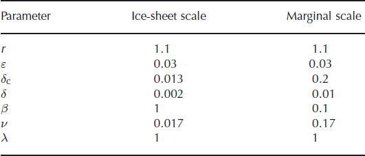
Some typical values for the parameters are given in Table 1, and the resulting values for the scaled variables and the dimensionless parameters are shown in Tables 2 and 3. Two particular situations are considered: first, for a large ice sheet we take Ψ0 = 10 Pa m − 1 and l = 1000 km; second, because much of the interest in subglacial drainage is focused on the region near the ice-sheet margin, we take typical values for a marginal area of Ψ0 = 100 Pa m − 1 and l = 100 km.
Table 1. Values used for the model constants. The ice viscosity is chosen based on a stress of 0.1 MPa using Glen’s flow law with A = 5 × 10⁻²⁴ Pa−3 s−1 at 0°C.For different stress conditions the effective viscosity could be somewhat different from this value, perhaps in the range η i ∼ 1012–1015 Pa s. The value for F uses a Manning roughness coefficient, n’ = 0.1 m − 1/3 s. The value for G is the global average geothermal heat flux. The roughness, R, and the permeability constant, k 0, are likely to depend strongly on the structure of the bed, with typical ranges perhaps R ∼ 10 − 3–10 − 1 and k 0 ∼ 10 − 6–10 − 1. The sliding velocity will usually be in the range u b0 ∼ 0–10 − 5 m s−1

Table 2. Values of model scales for either a whole ice sheet or the marginal region. The first four values are prescribed and the others then follow from Equations (13), (19) and (
26) and the values in Table 1. Values for Ψ0 = ρ
i
gH
0
/l and ![]() are based on an ice depth H
0
∼ 1000 m. The representative value for q
0 is chosen as that which would balance the melting term in Equation (8)
are based on an ice depth H
0
∼ 1000 m. The representative value for q
0 is chosen as that which would balance the melting term in Equation (8)

Table 3. Typical dimensionless parameter values corresponding to the scales shown in Table 2
It is useful to note from the scales in Equations (13) and ( 19) how the typical pressure depends on the discharge, and this is illustrated in Figure 3. A channel typically has a larger effective pressure (lower water pressure) for a larger discharge, whereas the porous flow has a smaller effective pressure. For large enough discharges this results in the channel drawing in water from the surrounding bed, and the amount that can feed into the channel is limited only by how large an area of the bed it is able to draw water from, which depends upon the efficiency of the distributed system at redirecting the water supply.

Fig. 3. Typical values of effective pressure as a function of discharge for a steady-state drainage system consisting of either a channel (N, dashed curve) or a distributed system (N c, solid curve) across a basin of width 10 km with potential gradient, Ψ = 9 Pa m−1.
If a channel is aligned with the ice flow, along y = 0 say, the distance over which the reduced pressure is felt can be seen immediately from the scaled equations: it is the length scale over which the transverse and downstream divergence of water flow balance in Equation (21). From Equation (22) the former is of size δN/y 2, whereas the latter is of size Ψ/x, so in order to balance their importance, the y-coordinate must be scaled by δ 1/2 (the dimensionless N, Ψ and x being ∼1). The dimensional distance over which the channel influences the surrounding porous flow is therefore of order

This is the length commonly referred to as the compaction length in analogous models for partially molten rock. For the values given above, it is ∼40 km in the case of the channel extending over the whole ice sheet or 10 km for just the marginal region. Since discharge generally increases from the interior towards the margins of the ice sheet (e.g. in Greenland the bed is thought to be frozen over much of the interior so there is no water there), there is probably only enough meltwater for channels to exist in marginal regions of ice sheets. This last value therefore gives an estimate for the predicted spacing of the channels.
If we know the spacing, δ 1/2 l, and the discharge in the distributed system, q 0, a sensible size to choose for the channel discharge is
Instability of distributed flow
An important thing to note from the scaled equations is that the heating due to the water flow in Equation (24) is unimportant compared with the ‘background’ melting due to the first two terms and with the additional opening due to sliding in Equation (23). Indeed, this is the fundamental distinction between distributed and channel drainage: in the former, the opening of the drainage space is essentially ‘passive’ – it does not depend on the flow rate; whereas for the latter the opening rate is ‘active’ – it is proportional to the flow rate.
By including the small viscous dissipation term in Equation (24), however, the model allows for the possibility that the distributed flow can become unstable. Combining the evolution equation (23) with Equations (22) and ( 24) gives
where the coefficients, c
1 = 1 + νub
·
τ
b + λ|ub
|, c
2 = ε|Ψ + δ∇N|
2
/β and c
3 = N, do not depend upon sheet depth, h. Linear stability analysis shows that the steady depth, ![]() , is therefore unstable to small perturbations if
, is therefore unstable to small perturbations if ![]() or, equivalently, if the steady discharge,
or, equivalently, if the steady discharge, ![]() , is larger than c
1Ψ/2c
2. In other words, a steady distributed flow will be unstable to perturbations in the sheet thickness if the discharge,
, is larger than c
1Ψ/2c
2. In other words, a steady distributed flow will be unstable to perturbations in the sheet thickness if the discharge, ![]() , becomes large enough that the dissipation term in Equation (23) is comparable with the other (passive) opening terms. Ignoring the small effective pressure gradient, the critical discharge is written dimensionally as
, becomes large enough that the dissipation term in Equation (23) is comparable with the other (passive) opening terms. Ignoring the small effective pressure gradient, the critical discharge is written dimensionally as
This instability is similar to that for a laminar sheet (Reference WalderWalder, 1982), except that the presence of the passive opening terms and the closure due to a positive effective pressure allow for the possibility of a stable state at low enough discharge (see also Reference Creyts and SchoofCreyts and Schoof, 2009). This suggests that as the discharge increases down-glacier, steady flow in a sheet will be viable until the critical discharge, q c, is exceeded.
Once this is the case, a small transverse perturbation to the depth will start to grow; the behaviour of the sheet then becomes effectively channel-like; the regions with larger h have a larger effective pressure, and therefore draw in water from the surrounding regions of smaller h. This has a runaway effect, however, and the equations exhibit a blowup that is common to many such nonlinear reactive/diffusive systems. In numerical calculations of Equations (21– 24), the depth of the sheet keeps growing and growing in a narrow band (the ‘channel’) of ever-decreasing thickness. This is indicative of an ill-posed mathematical model for which the fastest-growing instability occurs at the shortest wavelengths. At some stage in the channel’s growth, the porous model becomes an inadequate description of the dynamics, and it is necessary to switch to the channel model (Equations (15– 18) ). Since it is very thin compared to the scale of the distributed flow, the channel can then effectively be treated as a line sink, as is done for the calculations in the next section.
The critical discharge given by Equation (28) may be misleading however. It considers the case when the average dissipative heating across the distributed system becomes large enough to dominate the passive opening due to sliding and geothermal melting. In fact, a channel is likely to form when dissipative heating dominates over other opening mechanisms within an individual drainage component of the distributed system (Reference KambKamb, 1987). These may not necessarily be the same thing.
A second misleading feature of the linear stability criterion is that once a channel has formed it will tend to draw in the surrounding water, and in particular the water that approaches it from upstream. As shown in the Appendix, this inflow is effectively diffusive, and gives rise to a locally infinite (though integrable) flow into the head of the channel. The dissipative heating that results from this means the channel will melt (or ‘erode’) its way up the glacier, much like the headward erosion of a gully in overland flow. Numerical calculations of Equations (21– 24) show the channel growing in this way, but they are hampered somewhat by the need for very high resolution near the head of the channel (the dissipative heating term in Equation (24) is small), and the fact that an arbitrary switch must be made between the porous model and the channel model at some sheet depth. We cannot therefore calculate the rate of channel growth in this manner with any accuracy, although it is hoped that future work might study this in more detail.
In the rest of this paper we consider steady-state configurations for which a channel of fixed length is surrounded on either side by porous flow, and we calculate how the water moves into the channel. We do not concern ourselves with the dynamics of channel growth, and will therefore ignore the dissipative heating in the distributed system, since this only becomes important when it transitions to a channel (in the scaled Equations (21– 24) this corresponds to taking ε = 0).
Boundary conditions
The geometries considered are shown in Figure 4. It is natural to prescribe zero water flux, q = 0, at the upstream end of a catchment basin, x = 0, and to prescribe atmospheric pressure at the margin, x = l. If the ice depth goes to zero at the margin, however, this requires the effective pressure to be zero there, leading to unbounded growth of the drainage systems according to Equations (6) and ( 10). Several assumptions of the present model, in particular that the system is water-filled all the way to the margin, are invalid in this case (Reference Evatt, Fowler, Clark and HultonEvatt and others, 2006). It is therefore more appropriate to treat the ‘margin’ as a position slightly upstream of where the ice depth reduces to zero, and to apply the condition N = N m at x = l, where N m is a constant that represents the ice pressure at that point.

Fig. 4. Idealized geometry of a catchment basin considered for numerical solutions. Ice flow and the potential gradient are in the x-direction with x = l the ice margin, at which the effective pressure is prescribed. Boundary conditions in the y-direction are reflective, to represent the effect of a drainage divide between adjacent channels. A channel is treated as a line sink to the distributed flow, aligned along y = 0 for x > x c. The value of the effective pressure in the distributed system there must match with that in the channel.
In the next section a channel is assumed to lie along the line y = 0, starting at position x = x c, and it therefore requires boundary conditions Q = 0 at x = x c and N c = N m at x = l. The channel is treated as a line sink to the porous flow, so the pressure in the channel is prescribed as a boundary condition on the distributed model there, in the dimensionless variables:
(Note δ c /δ is the ratio of scales for the effective pressure in the channel and distributed system.) The dimensionless influx, Ω, to the channel can then be calculated (assuming symmetry between each side of the channel) as
Note that we ignore the effects of any ‘bridging stress’ (Reference Lappegard, Kohler, Jackson and HagenLappegard and others, 2006); in the vicinity of a low-pressure channel the average overburden must be spread over the surrounding area in contact with the bed, so that the local normal stress of the ice on the bed is large at the edges of a channel (Reference WeertmanWeertman, 1972). This effect could potentially be included by locally increasing the effective pressure in the closure term, Equation (11).
Results
Coupled channel and distributed flow
Figures 4 and 6 show an example of the coupled channel and distributed flow. We concentrate here on a marginal region, assuming the bed upstream of this is frozen, so that q = 0 at x = 0. The driving potential gradient is taken to be constant, Ψ = 1 non-dimensionally, and the predominant water source is from surface melting, ω = 1 non-dimensionally. This example is supposed to be representative, rather than to correspond to any particular geographic location, but it might be appropriate for the Greenland ice sheet, or for the margins of the former Laurentide ice sheet. The influx, Ω, from the surrounding porous flow is calculated from Equation (30) by solving Equations (21– 24), using the channel pressure, Equation (29), as a boundary condition; the channel pressure itself is calculated from the channel dynamics in Equations (15– 18). A cross-sectional profile for the same solution is shown in Figure 7.

Fig. 5. Steady-state solutions for (a) h and (b) N, to Equations (21– 24) with r = 1.1, ε = 0, δ = 0.01, β = 0.1, ν = 0.17 and λ = 1;plotted using the scales in Table 2 appropriate for the marginal region of an ice sheet. The driving potential gradient is constant, Ψ = 1 in the dimensionless variables, and there is a uniform source, ω = 1, from surface melting. No water is assumed to arrive from upstream of this region, so q = 0 at x = 0. A channel is prescribed to lie along y = 0, x > x c = 20 km, and the pressure within this (Equation (29)), is calculated from the rate of inflow (Equation (30)), using the steady-state channel equations (15– 18) with r = 1.1, ε = 0, δ c = 0.2. The boundaries in the y-direction are taken to be far enough away from the channel that the solution tends to one-dimensional flow through the distributed system there. The white arrows show the direction of water flow. The corresponding behaviour of the channel is shown in Figure 6 and a cross section along the dashed line in Figure 7.

Fig. 6. Steady-state solutions for the channel shown in Figure 4 showing (a) discharge, (b) cross-sectional area and (c) effective pressure. The dashed curves show analytical approximations based on the influx (Equation (A17) in Appendix). Note that the water goes back out into the surrounding bed near to the margin because the effective pressure in that boundary layer becomes larger than it is in the channel.

Fig. 7. Cross-sectional profiles of the drainage system depth, h, and effective pressure, N, on either side of a channel, along the line x = 65 km marked in Figure 4. The dotted line shows what the value would be for one-dimensional distributed flow.
We see that the large effective pressure in the channel influences the surrounding porous system and that the length over which it does this is of the order δ 1/2 l ≈ 10 km. Water is drawn inwards, but the compacting nature of the porous system means that close to the channel its depth decreases; it is squeezed nearly closed by the large effective pressures. Despite the transmissivity (∝ h 3) reducing in this way, the large pressure gradients are sufficient to draw the water through, and the channel captures almost all the water from the surrounding region. We anticipate that adjacent channels would therefore be spaced at a distance ∼δ 1/2 l, or perhaps slightly less.
Channel extent
As discussed previously, if dissipative heating in the distributed system is included in the model a channel can be expected to extend up the glacier due to melting at its head. The question then arises whether this process can continue indefinitely, so that a steady-state channel extends all the way to the ice divide, or whether it is limited at some stage by the supply of water from the surroundings. Intuition and field evidence from alpine glaciers suggest that channels should not be expected to extend indefinitely (though, as noted above, the varying melt input to alpine glaciers may be quite different from the steady input considered here). This is also evident from the model. Near the head of a channel its discharge is low, and the effective pressure is consequently low (Fig. 3). Thus, if the discharge in the channel were so small that the effective pressure were lower than it would be in the surrounding distributed system, it would flow back out to the surroundings and the channel would no longer exist there. There must therefore be a critical position for the channel head where the effective pressure is sufficiently elevated above the surrounding distributed flow to draw in just enough water to sustain the channel at that pressure. This position will depend upon the available water (the discharge, q) in the distributed system, and how efficiently it can be drawn into the channel.
One approach to find this position is to include the dissipation term in Equation (24) in numerical calculations for the porous flow around a channel and to allow the channel to lengthen as the sheet depth, h, grows near its head, continuing until a steady state is reached. The question of when to transition from sheet to channel model makes this approach difficult, however, and the results could only be given in terms of numerical solutions to a quite complex system of partial differential equations. A more satisfying and useful approach, which determines an explicit criterion for how far a channel can extend, is to use analytical methods to approximate steady flow into the channel, and use this to determine whether such a channel is viable. This is described in the Appendix; the analytical approximations are also shown in Figure 6. The approach is to solve approximately for what the flow, Ω, into the channel would be given its position, x c, and pressure, N c; then to solve for what the pressure, N c, should be given that influx, Ω, and thus to find the value of x c which makes these two calculations consistent.
The result is that the channel head should extend up-glacier as far as the discharge in the distributed system, ![]() (i.e. the one-dimensional solution that would occur in the absence of a channel), exceeds a critical value, q
*, given in dimensional variables by
(i.e. the one-dimensional solution that would occur in the absence of a channel), exceeds a critical value, q
*, given in dimensional variables by

Here C = 1.89 … is a constant, and W
O is the opening due to passive mechanisms in Equation (11) (i.e. W
O = (G + ub
·
τ
b)/ρ
i
L + R|ub
|). This is an algebraically messy criterion, but it essentially says that the available discharge must be sufficient to provide just enough dissipative heating to keep a channel open against viscous closure. Note that q* depends upon various parameters, but also potentially on position, through Ψ; the critical discharge is smaller where the potential gradient is larger. For a given discharge, ![]() , (which is determined by the meltwater supply), the position at which channels can begin, x
c, can be calculated from where
, (which is determined by the meltwater supply), the position at which channels can begin, x
c, can be calculated from where ![]() in Equation (31), and this determines the channel’s length, l
c (from x
c to the margin).
in Equation (31), and this determines the channel’s length, l
c (from x
c to the margin).
The condition given by Equation (31) represents one of our main conclusions. It suggests that the following factors tend to make channel transport more favourable:
-
the potential gradient is larger,
-
the rate of opening of the distributed system is slower,
-
the permeability of the distributed system is smaller,
-
the discharge is larger.
Any of these factors allow a channel to start further up-glacier.
Channel spacing
If the channel does not extend close to the full length of the catchment basin, l, it is possible to improve the estimate for the channel spacing (Equation (25)) by incorporating the length, l c, in the scaling argument. This is perhaps best explained by going back to the dimensional equations (8) and ( 9), where a balance of terms in the divergence of the discharge (which is essentially what determines the channel spacing, y c) requires

Here ![]() is the effective pressure in the distributed system
is the effective pressure in the distributed system ![]() and y
c is the channel spacing. Rearranging gives
and y
c is the channel spacing. Rearranging gives

in terms of dimensional variables. Since ![]() and Ψ will typically vary over the length of the channel (
and Ψ will typically vary over the length of the channel (![]() will be increasing and Ψ may also typically increase) this spacing also varies. In order to estimate the width of the channel’s catchment basin, we therefore take the average of this spacing over the length of the channel. The fact that Equation (33) decreases as both Ψ and
will be increasing and Ψ may also typically increase) this spacing also varies. In order to estimate the width of the channel’s catchment basin, we therefore take the average of this spacing over the length of the channel. The fact that Equation (33) decreases as both Ψ and ![]() increase suggests that channels will be more closely spaced near the margin, and therefore that new channels may initiate near the divide between two existing channels from further up-glacier. This makes some intuitive sense, and is in agreement with the observations and results of Reference Boulton, Hagdorn, Maillot and ZatsepinBoulton and others (2009).
increase suggests that channels will be more closely spaced near the margin, and therefore that new channels may initiate near the divide between two existing channels from further up-glacier. This makes some intuitive sense, and is in agreement with the observations and results of Reference Boulton, Hagdorn, Maillot and ZatsepinBoulton and others (2009).
The spacing in Equation (33) represents the most important result of this paper, and it follows simply from scaling arguments applied to the model equations. It shows that the spacing between adjacent channels of a given length will be larger if
-
the potential gradient is smaller,
-
the rate of opening of the distributed system is faster,
-
the permeability of the distributed system is larger,
-
the discharge is lower.
Thus, the properties that make channelized drainage start further up-glacier also make the channels more closely spaced; both are associated with inefficiency of the distributed system.
As an example, Figure 8 shows how the spacing between channels according to Equation (33) varies with the permeability constant, k 0, for an ice sheet of given shape and melt input. Varying k 0 can be thought of as a measure of how efficient the distributed system is at transmitting water. The length, l c, is first chosen according to Equation (31), and decreasing the permeability therefore has two competing effects on the channel spacing: first it allows for longer channels, which generally have a larger catchment basin (y c increases with l c), but, second, it limits the distance over which water can be collected, and therefore decreases the size of the catchment basin. The latter effect can be easily understood as due to the fact that a less permeable system requires larger effective pressure gradients to drive water through it, and the effective pressure maximum at the channel is therefore confined to a narrower region. As seen in Figure 8, the first effect is dominant when k 0 is larger and the second is dominant when k 0 is smaller.

Fig. 8. Extent of channels, l c, and channel spacing, y c, for varying permeability constant, k 0, as determined from Equations (31) and ( 33). This is for an ice sheet of length l = 1000 km from ice divide to margin, depth H 0 = 1 km, with surface z s = H 0(1 − x/l)1/2 and other parameters as given in Table 1. The solid curve shows the predicted channel length and spacing if discharge is assumed to increase linearly with distance from the ice divide up to q 0 = 2 × 10 − 4 m2 s − 1 at the margin and the dashed curves show the predicted length and spacing if melting does not start until the 200 km nearest the margin.
Ice-sheet drainage
Based on the previous discussion we now consider how the drainage system might look for an ice sheet with a more realistic shape, H = H 0(1 − x/l)1/2, giving rise to the potential gradient Ψ = Ψ0/2(1 − x/l)1/2. We first use Equation (31) to determine the length of channels, l c, and then use Equation (33) to determine the catchment basin width around each channel. We then calculate steady-state numerical solutions for the coupled flow in the distributed system and the channel, using reflective boundary conditions at the sides of the catchment basin, y = ±y c/2, to represent the divide between adjacent channels. Melting in the interior of the ice sheet is assumed to occur at a constant rate due to geothermal heating (see Tables 1 and 2 for the parameters used). The large discharge resulting from this melting gives rise to a wider channel spacing (∼32 km) than the typical 10 km quoted above. In reality one should, of course, have a non-uniform melting rate (with no melting over frozen parts of the bed); this example is again intended more as an illustration of the model than as pertaining to any particular real location.
Figures 9 and 10 show the results. The overall behaviour is most easily seen in Figure 10: the discharge over the whole width of the catchment basin is initially all contained in the porous system, until x c is reached when a large part of it moves into the channel.

Fig. 9. Steady-state solutions to Equations (21– 24), (29), (30) and ( 15–18) for (a) h and (b) N, with r = 1.1, ε = 0, δ = 0.002, δ c = 0.013, β = 1, ν = 0.017 and λ = 1, plotted in dimensional variables using the appropriate ice-sheet scales given in Table 2. The ice sheet has dimensionless potential gradient, Ψ = 1/2(1 − x)1/2, and geothermal and frictional heating result in a uniform meltwater source over the bed. The channel position is chosen using the critical discharge (Equation (31)), and the width of the catchment, y c, is chosen using Equation (33). Note the aspect ratio is exaggerated. The discharge and effective pressure in the channel are shown in Figure 10.

Fig. 10. (a) Total discharge (across the width of the catchment basin) carried by distributed system (solid curve) and channel (dashed curve), for the steady-state solution shown in Figure 9. The dotted curve shows the total discharge, which would be the distributed system’s discharge if there were no channel. The cross-sectional area of the channel near the margin is ∼12 m2. (b) Effective pressure in the channel (dashed curve), and averaged across the width of the catchment basin (solid curve). The dotted curve shows what the effective pressure would be if there were no channel.
Although the effective pressure in the channel is much larger than in the porous flow (Fig. 10b), it drops off quite quickly to either side so that the increase in the average effective pressure due to the presence of the channel is not perhaps as large as one might expect. One caveat, however, is that the size of the catchment area (over which this average is taken) has been chosen to be y c from Equation (25) based on scaling arguments. It is not clear that the catchment area should be exactly this size; it may be somewhat smaller (perhaps half the size) in which case the average pressure would be more influenced by the channel.
To illustrate the effect of surface melting, Figure 11 shows the steady-state solution for the same situation but with an additional supply of meltwater, ω = 10−9 m s−1, near the margin. When this extra water input reaches the bed, at x = 800 km, it begins to recharge the distributed system and only some of the additional supply (that closest to the channel) can be drawn into the channel. It is possible that another shorter channel might be viable at the drainage divide near the margin in this case, but this is not predicted in the solution since the dissipative heating term in the distributed system has been ignored.

Fig. 11. (a) Total discharge carried by distributed system (solid curve) and channel (dashed curve), for a steady state similar to that shown in Figure 10, except that an additional supply of water from surface melting, ω = 10−9 m s−1 (ω = 5 in the scaled variables), is included over the last 200 km near the margin. (b) Effective pressure in the channel (dashed curve) and averaged across the width of the catchment basin (solid curve).
Secondary instabilities
The critical condition on the discharge for channels to form (Equation (31)), can be generalized for water flow in the direction of a general potential gradient, Ψ + ∇N. That is, if the discharge through the distributed system, |q|, is larger than q* (based on the local potential gradient) then a channel is possible. Close to a major channel, for instance, the potential gradient is aligned towards the channel, and the resulting inflow of water will usually be sufficient to satisfy the critical condition. This suggests a secondary instability in which the flow into a main channel also evolves into channels, whose spacing will be given by a local equivalent of the compaction length (Equation (33)). The flow into these channels may also be subject to instability, so the resulting drainage pattern will be a branching network, similar to that shown in Figure 12.

Fig. 12. Possible structure of a channel network, with progressively smaller branches breaking off a main artery, formed by secondary and tertiary instabilities of flow into the main channel. Near the margin, larger quantities of meltwater and a steeper potential gradient reduce the size of the catchment basins (Equation (33)) so that smaller channels open up in between.
The presence of tributaries will allow for more efficient transfer of water into the main channels than has been calculated above. It also means that the larger effective pressures in the channel will be felt further out over the bed, so the average pressure is more influenced by the channel than is suggested in Figure 10b.
Eskers
Eskers are long sinuous ridges of sediment that are common in deglaciated regions of North America and northern Europe (Reference FlintFlint, 1930; Reference Prest, Grant and RamptonPrest and others, 1968). They are widely thought to be the casts of major subglacial channels, where sediment is deposited on the channel floor and gradually builds up over time (Reference ShreveShreve, 1985; Reference Clark and WalderClark and Walder, 1994; Reference BrennandBrennand, 2000). Although there is a suggestion that some eskers could form almost instantaneously during large floods (Reference ShawShaw, 1994), most are thought to have formed in a time-transgressive fashion, beneath slowly retreating marginal regions. This view requires esker-forming channels to be stable over many years (perhaps centuries) of ice retreat and suggests that only the largest dominant arteries in a drainage network will produce them. It also seems unlikely that channels misaligned with the ice flow could have produced significant eskers, because as the ice slides it alters the course of such channels and erodes most sediment deposits.
These considerations suggest that only the major channels aligned in the direction of the ice flow are likely to produce eskers (the solid lines in Fig. 12) and that the spacing between them should follow from Equation (33). This is in rough agreement with the observed 8–25 km spacing (Reference Boulton, Hagdorn, Maillot and ZatsepinBoulton and others, 2009). These implications are similar to those noted by Reference Boulton, Lunn, Vidstrand and ZatsepinBoulton and others (2007a,Reference Boulton, Lunn, Vidstrand and Zatsepinb, Reference Boulton, Hagdorn, Maillot and Zatsepin2009). Although they consider groundwater flow in the regions between channels, the main difference between our work and theirs is the criterion for where channels should form. In Boulton and others’ model a channel forms where the effective pressure reaches zero, whereas we require that the discharge reaches a critical level, q* , at which the heat generated by water flow is sufficient to keep a channel open against the creep closure of the ice.
Conclusions
We have presented simple model equations for channelized and distributed drainage systems, with the flow in a channel coupled to the surrounding distributed system. The distributed system is treated as a deforming porous medium, with ‘pore’ space being created through basal melting and sliding to form cavities, and being closed down by viscous compaction of the ice.
The pressure perturbation around a channel is felt over a width of the distributed flow termed the compaction length (Equation (33)), which gives a rough approximation for the predicted spacing between adjacent channels of ∼10 km. This spacing of major channels may be identified with the typical spacing of eskers. It is larger when the distributed system is more permeable and when the driving hydraulic gradient is smaller.
Once formed, channels can extend by headward melting, and will reach a steady state where the background discharge in the distributed system first reaches a critical level, given approximately by Equation (31); this suggests channel flow is more favourable when the hydraulic gradient is larger and when the distributed system is less permeable.
Drainage models that attempt to distinguish between channelized and distributed flow are typically forced to address the questions of when a transition occurs between the two, what the spacing of supposed channels is and how efficiently water is able to transfer into them. Although there are, of course, other factors that can affect the location of channels, such as bed topography or englacial conduits of surface melt reaching the bed, the ideas presented here give some insights into these questions.
It should be noted that this work has only considered a steady-state drainage system and ignored the potentially large variations that occur during summer melting. For that reason, the focus has been on ice sheets rather than alpine glaciers. The model posed here could be used to examine non-steady states, and therefore apply also to alpine glaciers, but the natural timescales for evolution are on the order of weeks to years. Any more sudden changes of water input may result in elastic uplift of the ice, which could be added to W O in Equation (10).
Acknowledgements
Some of this work formed part of a doctorate funded by the UK’s Engineering and Physical Sciences Research Council. I thank A. Fowler for many fruitful discussions. I am also grateful for the support of a Killam postdoctoral research fellowship at the University of British Columbia. Thanks also to the reviewers for helpful comments.
Appendix
Creep closure relationships
Here we describe the physical basis for the closure rates used in Equations (6) and ( 11). If a cylindrical cavity with radius R containing (inviscid) water at pressure p w is surrounded by viscous ice with far-field pressure p i, force and mass balance require the radial stress, σ rr = −p + 2η i∂u r /∂r, and radial velocity, u r, to satisfy
Integrating from r = R to r = ∞ gives
where S is the cross-sectional area. This gives the closure rate, ![]() , included in Equation (6).
, included in Equation (6).
If the porous system is considered to comprise small cylindrical tubes with cross-sectional areas Sk , the total area over a representative width of bed, W, would be Wh = ∑S k, and would close down at an overall rate

This motivates the choice of closure rate in Equation (11). If the pores are instead considered to be spherical in shape, the equivalent of Equation (A1) in spherical polar coordinates would be
and integrating the force balance gives the closure rate for the volume, Vk , as
Summing over many such volumes gives the same result for ![]() as in Equation (A3) up to a factor of 3/4. In fact, any self-similar pore shapes would give rise to a similar closure rate with a ∼1 multiplicative factor. The argument relies in part on the elements that make up the drainage system being sufficiently well separated that p
i represents an appropriate far-field pressure. It should also be noted that the effective viscosity of the ice, η
i, may be different over a channel and a distributed system (due to different strain rates); an alternative to the parameterization used in Equation (11) might be to include a multiplicative factor, μ ≤ 1, so that
as in Equation (A3) up to a factor of 3/4. In fact, any self-similar pore shapes would give rise to a similar closure rate with a ∼1 multiplicative factor. The argument relies in part on the elements that make up the drainage system being sufficiently well separated that p
i represents an appropriate far-field pressure. It should also be noted that the effective viscosity of the ice, η
i, may be different over a channel and a distributed system (due to different strain rates); an alternative to the parameterization used in Equation (11) might be to include a multiplicative factor, μ ≤ 1, so that
If the porous medium is made of sheets that have a much smaller depth, hk
, compared with horizontal extent, lk
, they may close down at rate ![]() . The overall closure rate in this case may have a more complicated dependence on the sheet depth than the linear relationship used in Equation (11) (e.g. Reference Creyts and SchoofCreyts and Schoof, 2009), and would require further details of the small-scale geometry to be determined.
. The overall closure rate in this case may have a more complicated dependence on the sheet depth than the linear relationship used in Equation (11) (e.g. Reference Creyts and SchoofCreyts and Schoof, 2009), and would require further details of the small-scale geometry to be determined.
In any case, the closure rate is expected to be an increasing function of both effective pressure and sheet depth and Equation (11) is the simplest parameterization with those properties.
Approximation for flow into a channel
Here we use Equations (21– 24) together with Equation (29) to approximate the steady inflow (Equation (30)), to the head of a channel at x = x c. The channel pressure, N c, is initially treated as known; once the influx has been calculated we can use the channel equations (15– 18) to determine what that pressure really is. Dissipative heating in the distributed system is ignored (by taking ε = 0), and the analysis is based upon the smallness of the parameters δ and δ c (see Reference HewittHewitt, 2009 for further details).
In the steady state, with Ψ = (Ψ, 0), Equations (21– 24) can be written as

where

is what the discharge would be in the distributed system in the absence of a channel (i.e. the one-dimensional solution) and W O = 1 + vub · τ b+λ|ub | is the opening rate (constant). The relationship (Equation (A8)) between N and h means Equation (A7) is a nonlinear diffusion equation for h (or N). We rescale the transverse coordinate to the width of the catchment area,
and then take only the leading-order terms in S. The resulting equation is most easily written in terms of q - h 3Ψ, the discharge in the x-direction:
The channel pressure condition, Equation (29), becomes

whilst the solution in the far field, as Y → ∞ , should tend towards the one-dimensional solution, ![]() . Equation (A11) can be solved approximately by writing the left-hand side as
. Equation (A11) can be solved approximately by writing the left-hand side as
and defining a distorted length variable

in place of x. Writing ![]() , the problem then reduces to
, the problem then reduces to

with ψ = 0 on ξ = 0, ψ → 0 as Y → ∞, and

where ξ c is the position of the channel head. This is a straightforward diffusion problem and the solution gives Ω (Equation (30)) as

Note that ψ
c defined in Equation (A16) depends upon both the far-field discharge in the distributed system, ![]() , and the channel pressure, N
c. This analytical approximation for the influx to the channel can be used in the channel equations (15–
18) to calculate Q, S and N
c, and these approximations are compared with the numerical solution in Figure 6.
, and the channel pressure, N
c. This analytical approximation for the influx to the channel can be used in the channel equations (15–
18) to calculate Q, S and N
c, and these approximations are compared with the numerical solution in Figure 6.
Near the head of the channel, where x is close to x c (ξ is close to ξ c), the dominant term in Equation (A17) is the first term, and gives rise to a channel discharge

where the constant A is given by

in which all the variables (![]() , Ψ, N
c) are evaluated at x = x
c. Now this discharge (which, remember, depends upon the unknown pressure N
c(x
c)) can be used in Equations (15–
18) to calculate the resulting channel pressure. In a steady state those equations reduce to
, Ψ, N
c) are evaluated at x = x
c. Now this discharge (which, remember, depends upon the unknown pressure N
c(x
c)) can be used in Equations (15–
18) to calculate the resulting channel pressure. In a steady state those equations reduce to

and we treat δ c as a small parameter. If Q takes the form in Equation (A18) near x c then the behaviour of N c there can be found by rescaling
and solving the resulting equation for ![]() ,
,

There is a unique initial value of ![]() at
at ![]() that matches this behaviour at infinity and this is found numerically to be B = 0.962 …. Thus the effective pressure at the head of the channel is
that matches this behaviour at infinity and this is found numerically to be B = 0.962 …. Thus the effective pressure at the head of the channel is
This gives an expression for the channel effective pressure, N
c(x
c), in terms of the influx, A(x
c), whilst Equation (A19) gives an expression for the influx dependent on that effective pressure; the two expressions must therefore be satisfied simultaneously. Whether a given location, x
c, is a viable position for the head of the channel is indicated by whether or not they can be solved. Considering the graphs of A against N
c defined by Equations (A19) and
(A23) and calculating when they intersect, a little algebra yields that they have a solution if the dimensionless discharge, ![]() , satisfies
, satisfies

where the constant C is

When converted back into dimensional variables this defines the critical discharge, q *, given in Equation (31).


