


Introduction
Worldwide urban population is projected to increase by nearly 2.5 billion people by 2050 [1], which will ultimately lead to increased congestion and demand for a significant enhancement of traffic management intelligence. One important building block toward the vision of Smart Cities is a comprehensive multimodal predictive routing including all means of transportation.
When focusing on road safety and efficiency, the actual challenge is to improve the overall usage of available public space by means of wide-area observation from the infrastructure side. Therefore, multiple sensors are mounted overhead at, e.g. roadside light posts or building walls to illuminate road and bike lanes, pedestrian crossings, or sidewalks beneath, with the aim of generating a complete ‘global’ real-time map of public-space usage. Depending on the type and required latency of information, these data may be processed locally or in a backend cloud service, and supplied to road users via suitable 802.11/V2X or mobile links.
Parking-space occupancy detection with the aim of optimized directed routing is one application supported by this new infrastructure. This problem has been addressed in the past by means of various technologies, such as magnetic field sensors, video, or ground radar [Reference Deng, Luo, Jiang and Luo2,Reference Wolff, Heuer, Gao, Weinmann, Voit and Hartmann3]. Radar technology has some notable advantages in this context like, for instance, reliability under unfavorable light or weather conditions and respect for the privacy rights of road users, since no images are recorded. In particular, the benefits of an overhead installation compared with ground single-spot radars include the ease of installation without the need for closing of the road or the parking space, the capability of monitoring multiple spots per sensor and the added value introduced by the possibility of simultaneously measuring through traffic, detecting jams, counting, or classifying road users including pedestrians on sidewalks.
Recent developments in deep learning algorithms, provide an excellent opportunity to leverage the potential of the sensors and augment the system with intelligent features for smart-city applications. Specifically, convolutional neural networks (CNN), which have become the state-of-the-art approach in classification tasks, can be used to interpret the data acquired by the sensor and classify the radar images.
Although such architectures date back to the end of the 1980s [Reference LeCun, Boser, Denker, Henderson, Howard, Hubbard and Jackel4], they did not receive major attention until 2012, with the success of the architecture based on CNNs proposed by Krizhevsky et al. for the Imagenet Large Scale Visual Recognition Challenge [Reference Krizhevsky, Sutskever and Hinton5]. Ever since, different variants of this concept have been proposed and applied in a wide variety of fields, including computer vision, natural language processing [Reference Kim6], drug discovery [Reference Wallach, Dzamba and Heifets7], etc.
The key aspect of their success is their ability to extract features from a hierarchical structure comprising several layers in order to solve non-linear problems more accurately than previous approaches based on feature design. All of this is done with a reasonable number of parameters, using local connectivity and shared weights.
Given their success, CNNs have also been considered for different applications in the radar field with very good results, especially in recent years. Some applications include spectrum sensing [Reference Zhang, Diao and Guo8], target detection [Reference Lopez-Risueno, Grajal and Diaz-Oliver9], automatic target recognition of SAR images [Reference Chen, Wang, Xu and Jin10], remote sensing [Reference Zhou, Wang, Xu and Jin11], and classification of micro-Doppler signatures in applications such as activity classification [Reference Kim and Moon12], hand-gesture recognition [Reference Kim and Toomajian13] or drone classification [Reference Kim, Kang and Park14].
In the following, we present an approach for occupancy detection of parking spaces using CNNs to classify images acquired by a radar sensor. To minimize the effect of irrelevant targets present in the scene, the system includes a background estimation algorithm to improve the classification performance. By leveraging the flexibility of CNNs, we introduce mechanisms to generalize the trained model and adapt it to new scenarios with very high accuracy and reduced training data. We present experimental results obtained in real parking scenarios which show the viability of our approach for its practical application.
Section “Radar sensor and parking scenario” describes the radar sensor and the signal preprocessing, while Section “Detection of stationary objects with background estimation” presents the background estimation technique for detecting stationary objects. The CNN architecture and the model-training technique are described in Section “Classifier based on convolutional neural networks”. Finally, Section“Experiments and results” presents an analysis of the results obtained in real parking scenarios.
Radar sensor and parking scenario
A schematic representation of the parking scenario is depicted in Fig. 1. The sensor is placed at a height h and a distance d from the area of interest; it is tilted with a pitch angle α in the elevation plane and perpendicular to the parking row. The sensor was designed at Siemens RF Systems labs and consists of 12 transmitters and 6 receivers forming a virtual uniform linear array of 72 virtual channels with a spacing of half a wavelength. The elements present a wide radiation pattern in azimuth but narrow in elevation to form a range-azimuth slice. To avoid country-specific frequency regulations, the radar operates at the 24 GHz ISM band, which, in addition, allows for a relatively wide bandwidth and the availability of highly integrated and mature radar ICs. An FMCW waveform with a bandwidth of 250 MHz at 24.125 GHz center frequency is used for each transmitter with a time-division multiplexing scheme and a sweep duration of 115.75 μs. The average output power is 12 dBm EIRP, and the typical operation range is 5–18 m. The multiple-input multiple-output (MIMO) configuration allows a reduction in terms of cost and size, since a filled array would require a geometrical extension of 35.5λ (as opposed to 20.5λ with the MIMO array) and the respective switching mechanism with 72 physical channels. Fig. 2 shows a block diagram of the hardware. The two-dimensional (2D) radar image is rendered after a complete sweep through all the transmitters, with an approximate period of 3 ms.
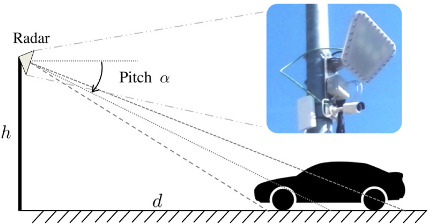
Fig. 1. Schematic representation of a downfire radar installation for parking monitoring.
Fig. 2. Block diagram of the switched MIMO radar sensor.
The frame rate of the sequence of images is set to four frames per minute to assure enough time resolution while maintaining a reduced throughput. In order to label the images of the training set and validate the classification result with ground-truth data, an IP camera is installed next to the sensor and synchronized to capture snapshots of the scenario at the same frame rate. The recorded data are transmitted via a point-to-point wireless link to a remote back-end for processing.
During the installation of the sensor, a calibration process is needed to obtain a local reference of the parking spaces with respect to (w.r.t.) the sensor. This process is carried out by measuring the coordinates of a corner reflector in different positions and is performed without altering the traffic or the parking scenario.
A slant-range image of the scenario is obtained by processing the raw data acquired by the sensor. For every virtual channel, each sweep is zero padded and windowed before performing a 2048-point fast Fourier transform with a Taylor window to obtain the range coordinates. The lateral resolution is achieved with digital beamforming using an azimuth sweep from − 60° to 60° with 1024 steps and a Chebyshev taper function with a side-lobe level of − 30 dB. These parameters were selected based on a criterion to maximize the signal-to-noise (SNR), while maintaining a constant side lode level and minimizing the variance of the mainlobe beamwidth across the azimuth span. The range-azimuth image is transformed into Cartesian coordinates, and the resulting image is resampled and interpolated in order to display a uniform rectangular grid in the x and y axes. During this transformation, the images are strongly oversampled w.r.t. the theoretical range and azimuth resolution. This is important because it allows the CNN to use several successive convolutional layers and downsampling operations to extract meaningful features.
Detection of stationary objects with background estimation
The average parking period can range from a few minutes to several hours depending on the nature of the scenario under consideration. Therefore, if a frame rate of the order of a few frames per minute is selected, the parking scenario can be considered static in the long term. This assumes that moving objects in an urban scenario, like passing traffic, a car during a parking maneuver or pedestrians, do not typically remain in the scene for more than a few frames.
Nonetheless, the appearance of such objects within the field of view of the sensor generates significant artifacts in the radar image of an otherwise static scenario. As is well known, the radial component of the velocity of moving targets w.r.t. the radar generates a Doppler shift that causes substantial alterations in the radar image [Reference Zoeke and Ziroff15]. This is due to the additional phase shift that is unaccounted for in the beamformer, and in a smaller scale, in the range dimension. These distortions have a big impact on the performance of the classifier, which is trained under the assumption of a static scenario, to minimize the amount of training data. For this reason, a background estimation technique is introduced to detect and track the regions of the image corrupted by this phenomenon, so that only those regions of the image that are regarded as static are processed, while the rest are not considered for classification.
We isolate the unwanted regions in the sequence of radar images with background estimation techniques that are similar to those widely used in computer vision for video-based applications [Reference Stauffer and Grimson16]. While spatial methods for background estimation analyse the image as a whole or blockwise by exploiting the spatial correlation of neighboring pixels, a temporal approach based on the statistical analysis of the history of each pixel is more suited for this application, given its robustness when dealing with very localized changes in the image [Reference Piccardi17]. Although the assumption of statistical independence between pixels does not accurately reflect the properties of the image, it is very beneficial when analyzing different regions of the image separately.
For a given pixel (x, y) of the image, at a time t, the probability of finding the intensity value X T = I(x, y, t) for a known pixel history χ T = {X t, …, X t−T} is given by P(X t |χ T), and based on this probability, the pixel is labeled as background or foreground. The evolution of the intensity values of each pixel along the time dimension is modeled with a Gaussian distribution. While a Gaussian mixture model is normally used in video applications to model different lighting conditions, the properties of the radar image makes the single Gaussian model more robust in terms of detection of foreground objects. After an initialization process to generate the model, the intensity value of each pixel in a new frame is checked against the model.
If a pixel does not match the model, it is labeled as foreground. A pixel matches the model if the following condition holds:
 $$ {X_t-\mu_{n,t} \over \sigma_{n,t}} \leq T_{\rm{model}}, $$
where μ n,t is the mean value of the n-th pixel at time t, σ n,t is the standard deviation and T model is the threshold which determines the sensitivity to foreground objects. A heuristic search for the value of this parameter shows that a typical value of T model = 2.5 represents a good trade-off between the number of discarded images and the accuracy of the classifier.
In order to adapt the model to the scenario dynamics, if a pixel matches the background model, it is updated according to a learning rate defined by the parameter α = 1/N, where N is the number of samples to compute the distribution parameters, typically N=12 frames. An online update scheme is deployed, as formulated in (2) and (3) to avoid buffering the last N samples of each pixel, thus significantly reducing memory requirements.
 $$ \mu_t = {{(N-1) \mu_{t-1} + x_t \over N}}, $$
 $$ \sigma_t = \sqrt{ {{(N-1) \sigma_{t-1}^2 + (x_t-\mu_{t-1}) (x_t-\mu_{t}) \over N}} }. $$
The proposed online approach allows the model to update in real time so that static objects fade into the background according to the time constant given by 1/α. This applies to newly parked cars that are integrated in the background model after a transient period and are considered static. The value of the time constant 1/α defines how fast the response time of this transient period elapses and depends on the scenario dynamics.
When a new frame is processed, the number of pixels labeled as foreground within each parking space is computed. If the percentage of the area with foreground pixels exceeds a given threshold (typically 25%), the parking space is discarded and is not classified.
Figure 3 depicts two typical scenes in a parking scenario: a static scene and a car during a parking maneuver. The background estimation process assures that the frames of interest contain only the information corresponding to static regions in the scenario, such that foreground objects, i.e. a parking space whose area contains more than 25% of pixels labeled as foreground due to short-term changes, is not considered for classification.
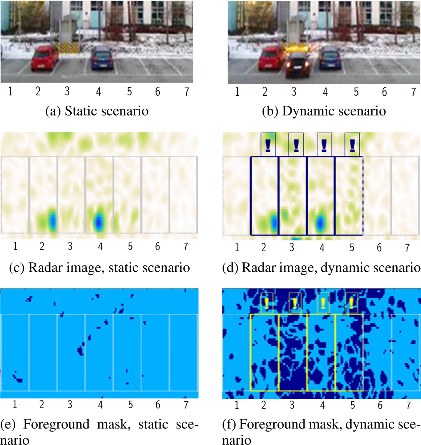
Fig. 3. Comparison between a static scenario (a) and a scene with a car during a parking maneuver (b). The radar image presents important distortions in the dynamic scenario (d) as opposed to the radar image in the static scenario (c). In the foreground masks (e,f), light blue represents the pixels that match the background model while dark blue represents changes in the scenario. The parking spaces with more than 25 % of foreground pixels (marked with an exclamation mark in (d) and (f)) are not considered for classification.
Classifier based on CNN
CNN architecture
After the background estimation process, the stationary images are fed into a binary classifier based on a CNN.
A CNN architecture is composed of several layers, such that higher layers represent higher levels of abstraction, which are capable of learning discriminative aspects from the raw input data without handcrafting-specific features for a particular problem [Reference LeCun, Bengio and Hinton18]. In general, the structure of a CNN consists of several functional blocks. Convolution filters are applied to extract local features from the input images. The filter size determines the size of the receptive field, and the number of filters represents the number of features to be extracted. A non-linear activation function, that activates when a given pattern is detected, is normally used. Pooling layers, which when combined with the convolutional filters obtain invariant translational and rotational features, are introduced to reduce the dimensionality. In a classification problem, the upper layers of the network often form a fully connected layer that links all the nodes in the previous layer with the class scores of the output layer using a softmax activation function.
Several architectures were tested during the experiments and evaluated in terms of classification accuracy and training time. A small CNN with three convolutional layers was selected due to the limited size of the training data. We used three convolutional layers with 10, 6, and 200 convolution filters, with dimensions 9 × 9, 5 × 5, and 6 × 6 pixels, respectively. After the first and second convolutional layers, a 2 × 2 max pooling layer was introduced, followed by a ReLU (rectified linear unit) activation function. These functions have proven to provide better convergence results compared with other functions, such as sigmoid or tanh functions [Reference Krizhevsky, Sutskever and Hinton5]. Finally, a fully connected layer is introduced to connect all the nodes in the last layer with two output classes, i.e. free/occupied parking space. For the output layer, we used a binary softmax regression that allows the output of each class (K = 1, 2) to be interpreted as a probability:
 $$\eqalign{ & \left( {\matrix{ {P(y = 1 \vert {\bf x};{\bf w})} \cr {P(y = 2 \vert {\bf x};{\bf w})} \cr } } \right) = \displaystyle{1 \over {\sum\limits_{k = 1}^K {\exp } ({\bf w}^T{\bf x})}}\left( {\matrix{ {\exp ({\bf w}_1^T {\bf x})} \cr {\exp ({\bf w}_2^T {\bf x})} } } \right),} $$
where x represent the outputs of the previous layer, and w = (w1, w2) is the matrix with the weights of the fully connected layer.
The cost function associated with this distribution is the binary cross-entropy loss, which is the function to minimize during the training stage. A regularization scheme was introduced by adding a weight decay term to the cost function to penalize large parameter values in order to reduce overfitting (λ = 0.0005):
 $$ \eqalign{ J({\bf w})= & -\sum_{m}\sum_{k}(y^{i}= =k)\log {{\exp({{\bf w}}^{T}_{k}{\bf x}) \over \sum_{\,j}\exp({\bf w}^{T}_{\,j}{\bf x})}} \cr &+ {{\lambda \over 2}}\sum_{k}\sum_{n}w_{k,n}^{2},} $$
where (y i = =k) is 1 when the label of the i-th training sample belongs to the class k and 0, otherwise.
Two dropout layers were introduced after the pooling layers for the same purpose: they randomly ignore connections between nodes with a probability of 50% during training. This is to prevent the formation of strong fixed connections derived from the particular characteristics of the training set, thus forcing the model to learn robust features that generalize better to new data. The CNN architecture is depicted in Fig. 4.
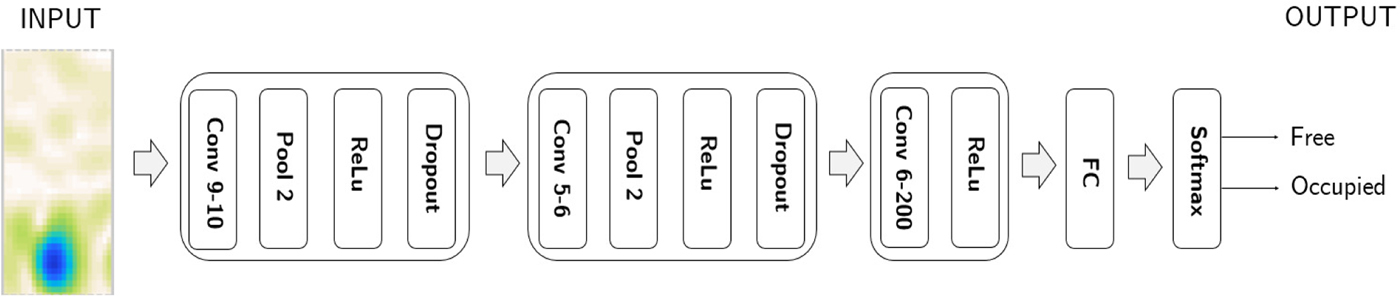
Fig. 4. Architecture of the CNN. The radar image of a single parking space is the input to the CNN. The two output classes correspond to the occupancy state of the parking space (free/occupied).
Training the model
The network is trained with experimental measurements from real parking scenarios. After generating the slant-range image of the scenario, the ground-truth coordinates of the parking lot w.r.t. the sensor are obtained during calibration, and the area in the image coordinates corresponding to each parking space is cropped and saved individually to train the network. As CNNs belong to a family of algorithms called supervised learning, the training stage requires labeled data. The image of each parking space is manually labeled according to its occupancy status (one free / two occupied). This is done for network training and results-analysis purposes.
We use an open-source framework for MATLAB® based on Caffe to implement the CNN [Reference Vedaldi and Lenc19]. During the training stage, the softmax layer is replaced by the binary cross-entropy loss function. An implementation of the backpropagation algorithm computes the gradient of the error w.r.t. the network parameters (i.e., the coefficients of the kernels in the convolutional layers and the weights of the fully connected layer), and a mini-batch stochastic gradient descent is used to minimize the cost function with a batch size of 50 images. To speed up convergence and reduce oscillations, the momentum method is applied with a weight of 0.9, while the learning rate is set to 0.001.
Generalization of the model
One of the drawbacks of applying CNNs to classify radar images is that, in general, there are not many labeled images available to train the network. Training a network of several layers with a reduced dataset often leads to parameters that overfit to the training set, thus degrading the cross-validation performance when evaluating test data from new scenarios. Clearly, to optimize the performance of the classifier for a given scenario, the network should be trained either with a very large and heterogeneous dataset or with training data from the specific location. Either way, the cost of acquiring labeled data for network training is very high in terms of time and labor, which renders the process unfeasible when deploying the system at a large scale. Furthermore, a challenge of this application is to account for the variability between scenarios, given the difficulty derived from the physical availability of mounting points, or permission for installation granted by different authorities or operators. While some generic CNN mechanisms try to minimize the impact of reduced training data by imposing architectural or algorithmic restrictions (dropout, regularization, etc.), other mechanisms based on the specific domain knowledge for the particular application can be incorporated in order to overcome the training-data challenge, and apply a general solution which makes the process viable from an economical perspective.
Dataset normalization
A critical preprocessing step before training the network consists of normalizing the intensity value of the training set. This allows the network to omit accidental features derived from the absolute backscattered intensity in a particular scenario and learn instead the characteristic geometric patterns in the 2D distribution of the power reflected by the object to be classified. By subtracting the mean value of the complete training set from each individual image, the power of the images is centered around zero. In a test scenario, the new images are zero-centered as well with the mean value of the images of the new scenario over a set period. The benefits of such a process are twofold. On the one hand, the variability between different scenarios is accounted for by minimizing the impact of differenft sensor setups, enforced by the particular requirements of a given scenario (the distance d to the parking row, the height h of the sensor and the pitch angle α). On the other hand, it reduces the effect caused by the directivity variation of the radiation pattern at different azimuth angles, which causes the images of the parking spaces near the boresight of the array to exhibit higher intensity than those at the outer limits of the azimuth field of view. In addition, this scheme provides the option of adapting to scenario variations over time (e.g. change of humidity, temperature, or nearby vegetation, which cause a certain drift of signal characteristics in the long term), by updating the mean value to zero-center the data.
Data augmentation
Given the sensor downfire orientation and the antenna array symmetry in the yaw axis, the imaging process presents a symmetry axis in the azimuth dimension, providing symmetry invariance to the classifier, such that its performance remains constant when the image is mirrored w.r.t. the range dimension. Although the CNN architecture could be modified to enforce such invariance, a method for artificially augmenting the dataset is much simpler, since it only requires understanding of the generative process of the data rather than the recognition process. Hence, the size of the training dataset can be artificially augmented by flipping the images on their respective vertical axes in a random subset of each batch during the backpropagation algorithm, and increasing the number of epochs. This operation is performed on 50% of the batch for each iteration.
Fine-tuning the model with a reduced dataset
As explained above, the option of training a network ad hoc with scenario-specific data is unrealistic in an industrial setting because a large dataset with thousands of labeled images of each scenario from different times of the day is required for optimal and stable sensor operation. Nevertheless, the performance of the classifier can easily be improved using a very small set of scenario-specific labeled data, provided that a model has been trained and tested with heterogeneous data. This can be done by loading a pre-trained model with sufficient data, and fine-tuning the weights by re-training the network with the reduced dataset for the specific scenario. The performance of this approach is discussed in Section “Scenario B versus fine-tuned model of scenario A”.
Experiments and results
The experiments were carried out in two different parking scenarios. The installation parameters in each scenario are listed in Table 1.
Table 1. Parameters of scenarios A and B
Scenario A
A first network is trained only with the data obtained in scenario A, which is an 80-m-long parking row. In this scenario, the region of interest in the radar image is restricted to a lateral coverage of seven parking spaces (roughly y ≈ ±9 m). We performed four sets of measurements along the whole parking lot in sub-scenarios of this size at different times on different days to introduce some variability into the model. The parameters d, h, and α were kept constant, except for instrumental errors caused by installing the sensor at different positions on different occasions (e d < 40 cm, e h < 40 cm and e α < 2°). For each set of measurements, the ground truth coordinates of the parking row w.r.t. the sensor were obtained during calibration, and the area in the image coordinates corresponding to each parking space is cropped and saved individually to train the network.
Each set of measurements takes 2 hours, and the total number of labeled images (after removing the non-static images detected with the background estimation technique) is about 11 000. We select a random subset of 2750 images (25 % of the whole set) to train the network. Although a limited amount of training data was used in the experiments, the tests show the viability of the proposed approach. Convergence was reached after 50 epochs and the training time was 370 s. Although considerable computational effort is required to train the network, especially if there is a large amount of training data involved, an image is classified in a single forward-pass through the network, whose parameters are pre-calculated. Hence, the complete detection operation can be run in real time: the scenario image is rendered at the required frame rate, the background is estimated, and the images for each parking space are then classified in the CNN. Fig. 5 depicts an example of the detected occupancy after classification.
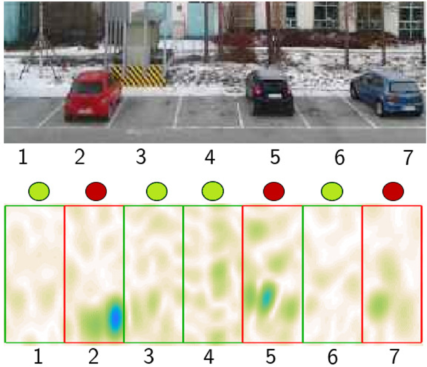
Fig. 5. Image of scenario A and the corresponding radar image after classification. Red markers indicate occupied parking spaces, while green ones show free spaces based on the classifier scores.
The performance of the classifier is assessed in terms of its classification accuracy (i.e. the ratio between the number of test images correctly classified and the total amount of labeled images), false positive rate, and false negative rate. The average classifier accuracy for the tested scenarios was 99.1%. Table 2 compares the results before and after using the background estimation technique, showing an improvement of about 3% when the images that contain foreground objects are not considered for classification. Fig. 6 shows the classification error for each parking space within the area of interest for one of the test scenarios with and without background estimation. The error distribution when no background estimation is applied depends on the dynamics of the particular scenario: there could be moving objects in random parking spaces, for example. When background estimation is enabled, however, a pattern emerges in which the error increases for those parking spaces further away from the boresight of the antenna. This is due to a reduction in the SNR caused by the loss of directivity of the beampattern at large scan angles.
Fig. 6. Classification error before and after background estimation.
Table 2. Scenario A
The rate of images discarded after the background estimation due to the artifacts caused by the Doppler effect, due to traffic and cars during a parking maneuver, was 5% in this scenario. It is worth pointing out that the ratio of the classifier accuracy and the number of discarded images greatly depends on the scenario dynamics, in such a way that in scenarios with heavy traffic, the rate of discarded images could increase to maintain a given classification accuracy level.
Scenarios B versus A
We evaluate the model's potential for generalization by applying the network trained on scenario A to the measurement data obtained on scenario B with a different sensor setup (Table 1). The number of available parking spaces in this scenario is limited to six cars; hence, the coverage of the radar image is reduced accordingly. We use a fixed installation and record the data over a 90-min period from the exact same location at different times on four different days.
In order to assess the generalization performance obtained with the mechanism of artificially augmenting the data by mirroring a random subset of each batch, we analyze the data when the network is trained without this mechanism. Table 3 indicates that the average accuracy obtained on scenario B with the model of scenario A without data augmentation is reduced to 90.3%. As expected, the accuracy is lower, as scenario A, where the network was trained, differs quite substantially from scenario B. However, when the network is trained with an artificially increased training set, we achieve an average improvement in classification accuracy of ~ 2.4%, which is consistent across the different sets of measurements recorded on scenario B.
Table 3. Scenarios B versus A
Scenario B versus fine-tuned model of scenario A
Finally, we analyze the classification performance when using a pre-trained model with heterogeneous data and fine-tuning the network with a reduced set of scenario-specific data, as discussed in Section “Classifier based on CNN”.
Specifically, we use the network for model A, which was trained with 2750 labeled images from four different days, and fine-tune the model by running backpropagation with a dataset of only 275 images from scenario B. The new dataset represents a 10% of the amount of images used to train the general model A. Due to the hierarchical representation of the features in a CNN, the lower layers should be practically unchanged after fine-tuning, while the weights of the upper layers are updated with the characteristics of the new dataset. To improve convergence in this context, the learning rate of the first layer is reduced from 0.001 to 0.0001.
The results from these experiments are shown in Table 4 and a snapshot of scenario B is depicted in Fig. 7. The accuracy obtained when the network for scenario A is fine-tuned with the reduced dataset from scenario B is 96.1%. If, however, the network is trained with such a reduced dataset from scratch, i.e. randomly initializing the weights without pre-loading the network of scenario A, the accuracy is reduced to 93.5%. This technique demonstrates the viability of generalizing a pre-trained model for new scenarios to very high accuracy levels without the need for acquiring and labeling a big set of training data from each scenario on different days. The cost of deployment in new scenarios with different environmental settings is thus significantly reduced.
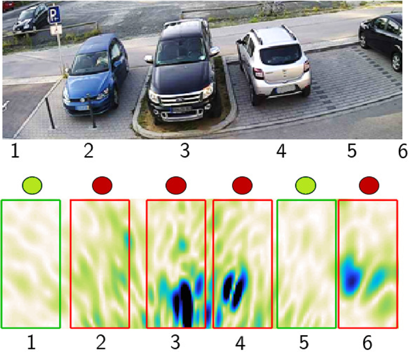
Fig. 7. Image of scenario B and the corresponding radar image after classification.
Table 4. Scenario B versus fine-tuned model of scenario A
Conclusion
We presented a method for monitoring parking spaces with a MIMO radar sensor in a downfire configuration. Foreground moving objects are detected and removed using a background estimation technique. The static background is classified using a CNN to determine the occupancy status of each parking space in real time. We introduce mechanisms to generalize the model for new scenarios by artificially augmenting the dataset and fine-tuning a pre-trained model with a reduced set of labeled data. Experimental measurements of different parking scenarios were presented showing very high accuracy and generalization capability after foreground objects have been removed, which shows the viability of the approach for its practical application. Future work will focus on rigorously testing these findings in already existing real-life pilot installations.
 Javier Martínez García received his Telecommunication Engineering degree in 2010 from the Universidad Autonóma de Madrid, Spain, and his Master's degree in 2013 from the Universidad Politécnica de Madrid. Between 2011 and 2015 he was employed by Indra Sistemas, where he worked on a number of R&D projects for radar and communication systems on the field of array processing. In September 2015, he joined the Institute of Microwaves and Photonics at Friedrich-Alexander University Erlangen-Nuremberg (FAU), Germany. His research interests include radar signal processing and convolutional neural networks.
 Dominik Zoeke received the Dipl.-Ing. degree in Information and Communications Technology in 2011 and is currently pursuing his Ph.D. in Electrical Engineering at the University of Erlangen-Nuremberg, Germany. Having a background in microphone array processing and acoustic localization, he joined the Radio Frequency Systems Department at Siemens AG Corporate Technology, Munich, Germany, as a Ph.D. researcher in 2011, where he is now working as an RF engineer on localization systems and signal processing for future industrial, traffic and smart city applications. His current research interests include radar sensor fusion and imaging, multivariate learning, and cognitive systems.
 Martin Vossiek received the Ph.D. degree from Ruhr–University Bochum, Germany, in 1996. He joined Siemens Corporate Technology, Munich, Germany, in 1996, where he was the Head of the Microwave Systems Group from 2000 to 2003. Since 2003, he has been a Full Professor with the Clausthal University of Technology, Clausthal-Zellerfeld, Germany. Since 2011, he has been the Chair of the Institute of Microwaves and Photonics, Friedrich-Alexander University of Erlangen–Nuremberg, Germany. His research has led to over 85 granted patents. He has authored or co-authored nearly 190 papers. His current research interests include radar, transponder, RF identification, and locating systems. Professor Vossiek is a member of the German IEEE Microwave Theory and Techniques (MTT)/Antennas and Propagation Chapter Executive Board. He was the Founding Chair of the MTT IEEE Technical Committee MTT-27 Wireless-Enabled Automotive and Vehicular Application. From 2013 to 2015, he was an Associate Editor of the IEEE Transactions On Microwave Theory and Techniques. He is a recipient of several international awards.


