


1. Introduction
The turbulent flow in the wake of large obstacles can nicely be visualised by the inhomogeneous distribution of aerosol particles (Kabanovs et al. Reference Kabanovs, Garmory, Passmore and Gaylard2019). A topical application is the highly inhomogeneous distribution of aerosol particles resulting when coughing without a mask (Chong et al. Reference Chong, Ng, Hori, Yang, Verzicco and Lohse2021), and the implications of this distribution on the spreading of infections (Memoli et al. Reference Memoli2015; Pujadas et al. Reference Pujadas, Chaudhry, McBride, Richter, Zhao, Wajnberg, Nadkarni, Glicksberg, Houldsworth and Cordon-Cardo2020), such as coronavirus (Morawska & Cao Reference Morawska and Cao2020).
Owing to the difference of the mass densities of the aerosol particles and the surrounding fluid, the particles follow slightly different tracks than the fluid (Cencini et al. Reference Cencini, Bec, Biferale, Boffetta, Celani, Lanotte, Musacchio and Toschi2006). This renders their flow field locally compressible and can lead to the emergence of finite time singularities (Gustavsson et al. Reference Gustavsson, Meneguz, Reeks and Mehlig2012) that are denoted as caustics (Wilkinson & Mehlig Reference Wilkinson and Mehlig2005). In addition to their role in infection spreading they are expected to play a role in the formation of rain droplets (Falkovich, Fouxon & Stepanov Reference Falkovich, Fouxon and Stepanov2002; Shaw Reference Shaw2003; Wilkinson, Mehlig & Bezuglyy Reference Wilkinson, Mehlig and Bezuglyy2006; Bec et al. Reference Bec, Ray, Saw and Homann2016; Ravichandran et al. Reference Ravichandran, Picardo, Ray and Govindarajan2022) due to enhanced collision rates (Ravichandran & Govindarajan Reference Ravichandran and Govindarajan2015), and hence for the modelling of precipitation in modern climate models (Ashwin et al. Reference Ashwin, Wieczorek, Vitolo and Cox2012; Schneider et al. Reference Schneider, Teixeira, Bretherton, Brient, Pressel, Schär and Siebesma2017; Prabhakaran et al. Reference Prabhakaran, Abu Sayeed Md Shawon, Thomas, Cantrell and Shaw2020). Moreover, the emergence of finite-time singularities in hydrodynamic flows is a problem in its own right in mathematical fluid dynamics (Ivanova & Gorman Reference Ivanova and Gorman1998).
Here, we follow up on a model of Wilkinson & Mehlig (Reference Wilkinson and Mehlig2005) that addresses caustic formation from a Lagrangian perspective: we address the time evolution of the mismatch of the velocity gradients of the particle field and the surrounding fluid in the immediate vicinity of a particle suspended in the flow. We consider the turbulent fluid-velocity field  ${{\boldsymbol {u}}}$ of the turbulent aerosol to be incompressible, isotropic and homogeneous at the relevant scales. The model is non-dimensionalised based on the Kolmogorov length scale $\eta$ and the inner velocity scale $u_{\eta }$ of the turbulent motion. In such a setting the gradient matrix $\boldsymbol{\mathsf{s}}_{ij} = \partial _i u_j$ of the fluid-velocity field ${{\boldsymbol {u}}}$ is driving the gradient matrix $\textsf{$\boldsymbol{\sigma}$} _{ij} = \partial _i v_j$ of the particle-velocity field ${{\boldsymbol {v}}}$ in the following nonlinear matrix equation
 \begin{equation} \frac{{{\mathrm{d}}} \textsf{$\boldsymbol{\sigma}$}}{{{\mathrm{d}}} t} ={-} \textsf{$\boldsymbol{\sigma}$} - \textsf{$\boldsymbol{\sigma}$}^2 + \boldsymbol{\mathsf{s}}, \end{equation}
where  ${{{\mathrm {d}}} \textsf{$\boldsymbol{\sigma}$} }/{{{\mathrm {d}}} t}$ is the material derivative of the gradient tensor of the particle-velocity field, $\textsf{$\boldsymbol{\sigma}$}$.
We demonstrate that (1.1) represents the dynamics of a noise-driven excitable system (Anishchenko et al. Reference Anishchenko, Astakhov, Neiman, Vadivasova and Schimansky-Geier2003; Lindner et al. Reference Lindner, García-Ojalvo, Neiman and Schimansky-Geier2004) such as they have been discussed in the context of activated decay of metastable states Graham (Reference Graham1990) and coherence resonance (Pikovsky & Kurths Reference Pikovsky and Kurths1997; Lindner & Schimansky-Geier Reference Lindner and Schimansky-Geier1999). From this perspective gradient-free particle flow,  $\textsf{$\boldsymbol{\sigma}$} =0$ is a global attractor of the deterministic dynamics, and the gradient matrix $\boldsymbol{\mathsf{s}}$ of the turbulent field serves as a noise term. Noise occasionally drives the dynamics over a manifold that discriminates between immediate decay towards $\textsf{$\boldsymbol{\sigma}$} =0$ and large excursions with a caustic, where $\text {Tr}(\textsf{$\boldsymbol{\sigma}$} )$ diverges.
This paper is organised as follows. In § 2 we derive the model equations. In § 3 we present an analytical solution of the evolution in the noise-free case, and discuss the properties of this dynamics. The statistics of caustics that emerge in the presence of noise is discussed in § 4. In § 5 we conclude the paper by a discussion of our results in the light of previous findings, suggestions for follow-up experimental and numerical studies, and a summary of our key findings.
2. The model
The present study address identical, small and heavy particles in a strong isotropic and homogeneous turbulent field. Moreover, we assume that the particles are smaller than the Kolmogorov scale of the turbulent flow. Consequently, the fluid flow is laminar on the scale of the particles, and the evolution of the particle velocity is described by the (dimensionless) Stokes equation
 \begin{equation} \frac{{{\mathrm{d}}} {{\boldsymbol{v}}}}{{{\mathrm{d}}} t} ={-} \left({{\boldsymbol{v}}}-{{\boldsymbol{u}}}\right) . \end{equation}
In Appendix A we revisit the derivation of this equation, and we discuss the constraints on the flow and particle properties where the (2.1) applies. Equation (1.1) is obtained by taking the gradient of (2.1).
2.1. Evolution of geometric invariants
Equation (1.1) describes a nine-dimensional dynamical system in three spatial dimensions. However, for an isotropic system only geometric invariants, i.e. combinations of the coefficients that are invariant under rotation of the coordinate system, carry physical information (Lumley Reference Lumley2007, appendix A2.6). These invariants amount to the coefficients  $c_k$ of the characteristic polynomial (2.2) of $\textsf{$\boldsymbol{\sigma}$}$ (cf. Lang Reference Lang1993; Garibaldi Reference Garibaldi2004; Lawson & Dawson Reference Lawson and Dawson2015),
 \begin{equation} P(\lambda) = \det( \lambda \boldsymbol{\mathsf{I}}_3 - \textsf{$\boldsymbol{\sigma}$} ) = \lambda^3 - X \lambda^2 + Y \lambda - Z \lambda^0, \end{equation}
where  $\boldsymbol{\mathsf{I}}_3$ is the $3\times 3$ identity matrix, and
 \begin{equation} X = \text{Tr}(\textsf{$\boldsymbol{\sigma}$}) , \quad Y = \frac{1}{2} \left(\text{Tr}(\textsf{$\boldsymbol{\sigma}$})^2 - \text{Tr}(\textsf{$\boldsymbol{\sigma}$}^2) \right) , \quad Z = \det(\textsf{$\boldsymbol{\sigma}$}) . \end{equation}
 The time evolution of  $X$ is found by taking the trace of (1.1). Due to the incompressibility of the fluid the noise term $\boldsymbol{\mathsf{s}}$ is trace-less and vanishes. Moreover, $\text {Tr}(\textsf{$\boldsymbol{\sigma}$} ^2)$ can be expressed in terms of $X$ and $Y$, yielding
 \begin{equation} \dot X ={-} X (1+X) + 2 Y . \end{equation}
 The time derivative of  $Y$ amounts to $\dot Y = X \dot X - ({1}/{2}) \, ({{{\mathrm {d}}}}/{{{\mathrm {d}}} t}) \text {Tr}(\textsf{$\boldsymbol{\sigma}$} ^2)$, and the time derivative of $\text {Tr}(\textsf{$\boldsymbol{\sigma}$} ^2)$ can be worked out by multiplying (1.1) by $\textsf{$\boldsymbol{\sigma}$}$ and taking the trace
 \begin{align} \dot Y &= X \dot X + \left( \text{Tr}( \textsf{$\boldsymbol{\sigma}$}^2 ) + \text{Tr}( \textsf{$\boldsymbol{\sigma}$}^3 ) - \text{Tr}(\boldsymbol{\mathsf{s}} \textsf{$\boldsymbol{\sigma}$}) \right) \nonumber\\ &={-}X^2 (1+X) + 2 X Y + X^2 - 2 Y + X (X^2-2Y) - X Y + 3 Z - \text{Tr}(\boldsymbol{\mathsf{s}} \textsf{$\boldsymbol{\sigma}$}) \nonumber\\ &={-}Y (2+X) + 3 Z - \text{Tr}(\boldsymbol{\mathsf{s}} \textsf{$\boldsymbol{\sigma}$}) . \end{align}
In the second step we used the Cayley–Hamilton theorem,  $P(\textsf{$\boldsymbol{\sigma}$} ) = 0$, to express $\text {Tr}( \textsf{$\boldsymbol{\sigma}$} ^3 )$ in terms of $X$,
$X$,  $Y$ and $Z$.
$Z$.
To derive the temporal evolution of  $Z$ we multiply (1.1) with $\textsf{$\boldsymbol{\sigma}$} ^{-1}$, take the trace and use Jacobi's formula:
 \begin{equation} \text{Tr}( \log(\textsf{$\boldsymbol{\sigma}$})) = \log(\det(\textsf{$\boldsymbol{\sigma}$})). \end{equation}
Hence, we find
 \begin{equation} \dot Z = Z \frac{{{\mathrm{d}}}}{{{\mathrm{d}}} t} \log Z = Z \text{Tr}\!\left( \textsf{$\boldsymbol{\sigma}$}^{{-}1} \frac{{{\mathrm{d}}}}{{{\mathrm{d}}} t} \textsf{$\boldsymbol{\sigma}$} \right) ={-}Z \left(3+X\right) + \text{Tr}\left( \boldsymbol{\mathsf{s}} \textsf{$\boldsymbol{\sigma}$}^* \right) , \end{equation}
where  $\textsf{$\boldsymbol{\sigma}$} ^*= Z \textsf{$\boldsymbol{\sigma}$} ^{-1}$ is the conjugate matrix of $\textsf{$\boldsymbol{\sigma}$}$.
As a final remark we note that two-dimensional turbulence may be considered as flow in a plane where all perpendicular velocity components vanish. In that case also their gradients vanish, and consequently also the determinant  $Z$ of the gradient matrix. Moreover, by a straightforward calculation, one verifies that $Y$ is the determinant of the non-vanishing $2\times 2$ sub-matrix of $\textsf{$\boldsymbol{\sigma}$}$. Therefore, (2.4a) and (2.4b) with $Z=0$ provide the description of inertial particles in two-dimensional turbulence. In the one-dimensional case (2.4a) with $Y = 0$ and $Z = 0$ reduces to a well-studied one-dimensional model to study caustics (Gustavsson & Mehlig Reference Gustavsson and Mehlig2016).
The dynamical system (2.4) constitutes a nonlinear stochastic differential equation in a Lagrangian point of view when  $\text {Tr}( \boldsymbol{\mathsf{s}} \textsf{$\boldsymbol{\sigma}$} )$ and $\text {Tr}( \boldsymbol{\mathsf{s}} \textsf{$\boldsymbol{\sigma}$} ^* )$ are interpreted as noise terms acting on the $Y$ and $Z$ dynamics, respectively. These coupling terms model the inertial effects of the turbulent dynamics, inducing the deviation of the particle from the fluid dynamics.
3. Deterministic evolution
To gain a qualitative insight into the formation of caustics in turbulent aerosols we analyse the model first in the absence of noise. The deterministic evolution of (2.4), that results when the noise terms  $\text {Tr}( \boldsymbol{\mathsf{s}} \textsf{$\boldsymbol{\sigma}$} )$ and $\text {Tr}( \boldsymbol{\mathsf{s}} \textsf{$\boldsymbol{\sigma}$} ^* )$ are dropped, describes the relaxation of the gradients of the particle flow field, $\textsf{$\boldsymbol{\sigma}$}$, towards those of the turbulent flow, $\boldsymbol{\mathsf{s}}$. It takes the form
 \begin{gather} \dot X(t) ={-} X(t) \left( 1 + X(t) \right) + 2 Y(t), \end{gather}
 \begin{gather}\dot Y(t) ={-} Y(t) \left( 2 + X(t) \right) + 3 Z(t), \end{gather}
 \begin{gather}\dot Z(t) ={-} Z(t) \left( 3 + X(t) \right). \end{gather}
This dynamical system can be integrated, taking the solution
 \begin{gather} X(t) = \frac{3 C_0 -2 C_1 \, {\rm e}^t - C_2 \, {\rm e}^{2t}}{ -C_0 + C_1 \, {\rm e}^t + C_2 \, {\rm e}^{2t} + C_3 \, {\rm e}^{3t} }, \end{gather}
 \begin{gather}Y(t) = \frac{-3 C_0 + C_1 \, {\rm e}^t }{ -C_0 + C_1 \, {\rm e}^t + C_2 \, {\rm e}^{2t} + C_3 \, {\rm e}^{3t} }, \end{gather}
 \begin{gather}Z(t) = \frac{1}{ -C_0 + C_1 \, {\rm e}^t + C_2 \, {\rm e}^{2t} + C_3 \, {\rm e}^{3t} } \end{gather}
with integration constants  $C_0$, $C_1$, $C_2$ and $C_3$ that are related to the initial condition $(X_0,Y_0,Z_0)$ of a phase-space trajectory at reference time $t=0$ by
 \begin{gather} C_0 = Z_0, \end{gather}
 \begin{gather}C_1 = Y_0 + 3 Z_0, \end{gather}
 \begin{gather}C_2 ={-} (X_0 + 2 Y_0 + 3 Z_0), \end{gather}
 \begin{gather}C_3 = 1 + X_0 + Y_0 + Z_0. \end{gather}
This system models caustic events when the denominators of (3.2) vanish, i.e. at finite times  $t=t_c$ where
 \begin{equation} C_0 = C_1 \, {\rm e}^{t_c} + C_2 \, {\rm e}^{2 t_c} + C_3 \, {\rm e}^{3\, t_c} . \end{equation}
While substituting  $E_c=e^{t_c}$ in this equation, we can calculate the finite caustic times $t_c$ at which a caustic occurs by solving the cubic polynomial
 \begin{equation} 0 = C_3 E_c^3 + C_2 E_c^2 + C_1 E_c - C_0 . \end{equation}
Solving for the times  $t_c$ reveals a remarkable feature of caustics. The relaxation of the excited trajectory to the global attractor at the origin will encounter a divergence for each real root of the polynomial (3.5) with $t_c > t_0$. Hence, the relaxation may involve up to three singularities with a specific progression of times and phase-space directions on the approach to the divergence. In the following, a caustic whose relaxation involves $\nu$ divergences will be denoted as ( $\nu$)-caustic.
Next we analyse the structure of the flow for this three-dimensional model so that we can understand how events such as (3)-caustics can emerge. Then we identify reduced two- and one-dimensional models that will allow us to discuss certain features in a simpler setting.
3.1. The flow upon approaching a caustic
The deterministic dynamical system (3.1) has fixed points at
 \begin{equation} P_0 = (0,0, 0) , \quad P_1 = ({-}1,0, 0) , \quad P_2 = ({-}2,1, 0) , \quad P_3 = ({-}3,3,-1) . \end{equation}
There is a remarkable correspondence between triples of these points and the constants  $C_0, \ldots, C_3$: $C_0 = 0$ determines trajectories in the plane $Z_0 = 0$ spanned by $P_0$, $P_1$, $P_2$; $C_1 = 0$ determines trajectories in the plane $Y_0 = -3 Z_0$ spanned by $P_0$, $P_1$, $P_3$; $C_2 = 0$ determines trajectories in the plane $X_0 = - 2 Y_0 -3 Z_0$ spanned by $P_0$, $P_2$, $P_3$; $C_3 = 0$ determines trajectories in the plane $Y_0 = -1 -X_0 -Z_0$ spanned by $P_1$, $P_2$, $P_3$.
The explicit solution (3.2) implies that these are invariant planes of the dynamics. Trajectories that start in one of the planes will stay in the plane, and trajectories that start in the intersection of any pair of these planes have a dynamics on a straight line defined by the intersection of the planes. Therefore, also the straight lines through any two of the fixed points are invariants of motion. Linear stability analysis reveals that the flow along these lines is oriented such that  $P_i$ has $i$ unstable directions. In particular, $P_0$ is linearly stable.
For  $C_3 \neq 0$ and $t \to \infty$ the denominators of (3.2) increase faster than the numerators. Hence, $P_0$ is a global attractor of the dynamics which renders the particle velocity field incompressible i.e. where particles follow the surrounding fluid. Almost all trajectories will approach the origin. Trajectories in the half space that contains the origin can approach zero without divergence. Trajectories in the plane $C_3 = 0$ will either approach $P_1$ or $P_2$. Trajectories on the opposite side of that plane will encounter a root of the denominator at some finite time $t_c$, that leads to a flip of the signs of $X$,
$X$,  $Y$ and $Z$. This finite-time singularity amounts to a steepening of the slope. The velocity gradients diverge and change sign. Similar events happen in wave breaking, and in the formation of caustics in optical reflections (Berry Reference Berry1976; Beven Reference Beven2019). An initial condition $(X_0, Y_0, Z_0)$ will undergo $0 \leq \nu \leq 3$ caustics when the polynomial has $\nu$ real roots with ${E_c} = \exp (t_c) > 1$, and it has undergone $0\leq \nu _p \leq 3-\nu$ caustics when the polynomial has $\nu _p$ roots with $0<{E_c}<1$.
There are regions where (1)-caustics occur. Furthermore, there is a phase-space region where (2)-caustics occur and a region where (3)-caustics occur. (3)-caustics are thereby defined by phase-space trajectories that diverge three times before they approach the global attractor  $P_0$.
The topological constraints on the flow stipulate that the domains of different types of trajectories are separated by the four invariant planes spanned by triples of three fixed points, and by the manifolds where cubic polynomial has double and triple roots.
The solutions, (3.2), of the deterministic dynamics, (3.1), are ratios of polynomials in the variable  ${{\mathrm {e}}}^t$. In the generic case the roots of the numerator and denominator are distinct. In that case there are numbers $\alpha$ and $\beta$ such that the approach to the singularity is always linear in leading order,
 \begin{equation} \lvert X(t) \rvert \gg 1 \quad \Rightarrow \quad Y(t) \sim \alpha X(t) \quad \land \quad Z(t) \sim \beta X(t) . \end{equation}
Far away from the origin the evolution of the trajectory towards a caustic follows a straight line to infinity with  $X(t) \to -\infty$ with some values $\alpha, \beta \in \mathbb {R}$. Interestingly, there are infinite many possibilities of a caustic to occur because $\alpha$ and $\beta$ are real parameters. Then it returns from the exactly opposite position in the three-dimensional phase-space. It still follows (3.7) with the same numbers $\alpha$ and $\beta$, and $X(t) \gg 1$ and decaying. Subsequently, the phase-space trajectory either goes through another caustic, where $\alpha$ and $\beta$ take other values, or it settles down to the origin. A trajectory can undergo at most three caustics, that correspond to the three roots of the denominator of (3.2).
The deterministic dynamics (3.1) always ends up asymptotically in the global attractor  $P_0$ and is therefore not chaotic.
3.2. Caustics in the two-dimensional model
It is instructive to note that the  $(X,Y)$-plane is an invariant manifold of the three-dimensional dynamics (3.1), and that this manifold is attractive as long as $X > -3$. Basic features of the dynamics can therefore be understood already in the two-dimensional dynamics where it is much easier to visualise the structure of the flow. For $Z \equiv 0$ the two-dimensional deterministic dynamics
 \begin{gather} \dot{X}(t) ={-}X(t) \left( 1 + X(t) \right) + 2 \, Y(t), \end{gather}
 \begin{gather}\dot{Y}(t) ={-}Y(t) \left( 2 + X(t) \right) \end{gather}
has solutions
 \begin{gather} X(t)= \frac{-2c_0- c_1 \, {\rm e}^t }{ c_0 + c_1 \, {\rm e}^t + c_2 \, {\rm e}^{2t} }, \end{gather}
 \begin{gather}Y(t) = \frac{c_0}{ c_0 + c_1 \, {\rm e}^t + c_2 \, {\rm e}^{2t} } \end{gather}
with  $c_0$, $c_1$, $c_2$ determined by the initial condition $(X_0,Y_0)$ of a phase-space trajectory at time $t=0$,
 \begin{equation} \left. \begin{aligned} c_0 & = Y_0,\\ c_1 & ={-} (X_0+2 Y_0)\\ c_2 & = 1+X_0+Y_0 . \end{aligned} \right\} \end{equation}
This dynamics has fixed points at
 \begin{equation} Q_0 = (0,0) , \quad Q_1 = ({-}1,0), \quad Q_2 = ({-}2,1) , \end{equation}
i.e. the fixed points  $P_0$, $P_1$, and $P_2$ of (3.6a–d) with $Z=0$. Accordingly, the invariant manifolds of the two-dimensional system are straight lines through every pair of these fixed points, and the flow along these lines is orientated such that $Q_i$ has $i$ unstable directions.
During a caustic the phase-space trajectories are to leading order linear functions with slope  $\gamma$ such that
 \begin{equation} Y(t) \sim \gamma X(t) , \end{equation}
and there are periodic boundary conditions in the variables  $X$ and $Y$ during a caustic at infinity.
The flow field, the invariant lines and the fixed points are shown in figure 1. This figure nicely shows that the origin is an attractor of the flow. Small finite excitations from zero decay right away, as long as they amount to initial conditions to the upper right of the manifold spanned by  $Q_1$ and $Q_2$,
 \begin{equation} Y ={-}1-X \end{equation}
that is marked by a solid red line. However, the trajectory makes a large excursion when their initial conditions are located below the red line (3.13). In particular, it must then go through a caustic before it can return to the origin. Different trajectories with initial conditions below the red line (3.13) are shown in figure 2. One can see that they have to perform a caustic event until the relaxation towards the global attractor sets in. At the global attractor the particle velocity fields is incompressible and no further caustic events can occur.

Figure 1. The flow field, the invariant lines and the fixed points. Arrows show the direction of the flow field of (3.8) in the  $(X,Y)$-plane. The speed of the flow is provided by a colour coding with a label provided by the bar to the right. The three fixed points $Q_0$, $Q_1$ and $Q_2$ are marked by a red $\boldsymbol {+}$, a green $\blacksquare$ and a blue $\bullet$, respectively. The invariant lines that proceed through all pairs of fixed points are marked by solid lines where the colours serve for a better visualisation.

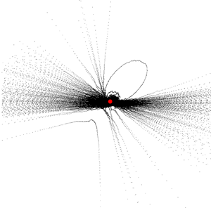
Figure 2. Different types of caustics in the two-dimensional model. The dashed, dash-dotted and dotted line show trajectories featuring a ( $1^-$)-caustic, a ( $1^+$)-caustic and a 2-caustic, respectively.
Similar to the three-dimensional system one can classify the trajectories based on the roots of the common denominator  $Y_0 - (x_0 + 2 Y_0) \exp (t) + (1 + X_0 + Y_0) (\exp (t))^2$ of the solutions (3.9). The denominator is a quadratic function in $\exp (t)$ with roots ${E_c}=\exp (t_c)$. The polynomial has a double root at $Y_0 = X_0^2/2$ (yellow line in figure 2). Trajectories undergo $0 \leq \nu \leq 2$ caustics if the denominator has $\nu$ roots with ${E_c} > 1$, and they experienced $0 \leq \nu _p \leq 2-\nu$ caustics in their past when the denominator has $\nu _p$ roots with $0<{E_c}<1$. A straightforward, even though tedious calculation provides a classification that can also be inferred for the inspection of the flow (figure 1).
(i) For initial condition with $X_0 < -1$ and $Y_0 = 0$ there are roots with ${E_c} = 0$ and ${E_c}>1$, respectively. These initial conditions lie on trajectories that started close to $Q_1$, and they undergo a single caustic where they diverge towards the left. They return from the right, and converge towards $Q_0$.
(ii) For initial condition with
$X_0 < -1$ and $0 < Y_0 < -1-X_0$ there are roots with ${E_c} < 0$ and ${E_c}>1$, respectively. These initial conditions lie on trajectories that started close to $Q_2$, and they undergo a single caustic where they diverge towards the upper left. They return from the lower right, and converge towards $Q_0$. These trajectories are said to exhibit ($1^+$)-caustics. An example is provided by the dash-dotted line in figure 2.(iii) Initial conditions with
$X_0 > -1$ and $0 \geq Y_0 > -1-X_0$ amount to post-caustic locations on the trajectories described in (i) for $Y_0=0$ and (ii) for $Y_0>0$, respectively.(iv) Initial conditions with
$X_0 < -2$ and $Y_0 = -1-X_0$ proceed along the red line, originating at $P_2$, diverging to the upper right and then approaching $P_1$ along the red line.(v) For initial condition with
$-1-X_0 < Y_0 < X_0^2/2$ there are two roots with ${E_c}>1$. These initial conditions lie on trajectories that started close to $Q_2$, undergo a caustic where they diverge towards the upper left. They return below the red line from the lower right, undergo another caustic towards the lower left and then they converge towards $Q_0$. These trajectories are said to exhibit (2)-caustics. An example is provided by the dotted line in figure 2.(vi) Initial conditions with
$Y_0<0$ and $Y_0 < -1-X_0$ amount to points in between the two caustics the former trajectories. Trajectories initialised at these points perform a ($1^-$)-caustic (dashed line in figure 2). The vast majority of noise-induced caustics is of this type.(vii) For
$X_0<-2$ and $Y_0 = X_0^2/2$ the trajectories are initiated on the line where the denominator has a double root. They evolve towards the upper left along the parabola indicated as solid orange line in figure 2, and subsequently they approach $Q_2$ along the positive branch of the parabola. This special trajectory separates the region where initial conditions perform two caustics, and where they return to the origin without undergoing a caustic.(viii) All other initial conditions approach directly
$Q_0$ without undergoing caustics.


3.3. Caustics in the one-dimensional model
The explicit solutions of the deterministic evolution imply that caustics involve a divergence of the divergence,  $X=\boldsymbol {\nabla } \boldsymbol {\cdot } {{\boldsymbol {v}}}$, of the particle velocity field, ${{\boldsymbol {v}}}$ (Wilkinson & Mehlig Reference Wilkinson and Mehlig2005; Wilkinson et al. Reference Wilkinson, Mehlig and Bezuglyy2006). A first impression on the aerosol dynamics can then be obtained by considering only the one-dimensional dynamics along the invariant manifold $Y_0=Z_0=0$ (Gustavsson et al. Reference Gustavsson, Meneguz, Reeks and Mehlig2012; Gustavsson & Mehlig Reference Gustavsson and Mehlig2013, Reference Gustavsson and Mehlig2016)
 \begin{equation} \left. \begin{gathered} \dot X(t) ={-} X(t) \left( 1 + X(t) \right) ={-} \frac{{{\mathrm{d}}}}{{{\mathrm{d}}} X} \varPhi( X(t) )\\ \text{with}\ \varPhi(X) = \frac{X^2}{6}( 3 + 2 X ) . \end{gathered} \right\} \end{equation}
For the initial condition  $X(0) = X_0$, (3.14) has the solution
 \begin{equation} X(t) = \frac{ X_0 }{ (1+X_0) \, {{\mathrm{e}}}^t - X_0 } \end{equation}
and the system undergoes a caustic when  ${E_c} = \exp (t_c) = X_0 / (1+X_0) > 1$, i.e. for initial condition $X_0 < -1$ where $X=0$ corresponds to the unstable point of the one-dimensional dynamical system. For $X_0>0$ the trajectory underwent a caustic in the past, and for $-1< X_0<0$ the trajectories relax directly towards the stable fixed point at the origin.
At this point we provide another property for the analysis of caustics, the caustic duration  $T_c$. As the formulas are quite easy for the one-dimensional system we provide it first here. A similar and straightforward calculation holds true also in the two- and three-dimensional cases. An estimation for the duration of caustic events is especially interesting for the next section where we analyse the effects of applying noise to the deterministic dynamics, i.e. (2.4). The duration of a caustic will be defined as the time $T_c$ where the particle proceeds in a region $X \not \in [-X_D, X_D]$ where the forcing due to the noise is negligible as compared with the deterministic force due to the steep decay of the potential $\varPhi (X)$. From (3.15) one infers that
 \begin{equation} X_D = \frac{ -X_D }{ (1-X_D) \, {{\mathrm{e}}}^{\langle T_c \rangle} + X_D } \quad \Rightarrow \quad \langle T_c \rangle = \ln \frac{ -1 -X_D }{ 1 - X_D } . \end{equation}
Here,  $X_D$ is a user-defined parameter and typically values are $X_D > 1$. In a case with noise this parameter will depend on the noise strength of the turbulent flow field. It can be determined by analysing when the phase space trajectories approach straight lines in the mean, i.e. when trajectories during a caustic stay in a cylinder of some fixed diameter $\delta$. As a remark, in the two- and three-dimensional cases one finds curves $Y_D(X_D)$ and planes $Z_D(X_D,Y_D)$, respectively.
4. Noise-induced caustics
Adding noise turns (3.1) into an excitable dynamical system (2.4) (Lindner et al. Reference Lindner, García-Ojalvo, Neiman and Schimansky-Geier2004). To gain insight into its dynamics we assume white noise terms
 \begin{gather} \text{Tr}(\boldsymbol{\mathsf{s}} \textsf{$\boldsymbol{\sigma}$}) \equiv \sqrt{2 D_1} \epsilon_1(t), \end{gather}
 \begin{gather}\text{Tr}(\boldsymbol{\mathsf{s}} \textsf{$\boldsymbol{\sigma}$}^*) \equiv \sqrt{2 D_2} \epsilon_2(t), \end{gather}
with delta-correlated Gaussian white noise  $\epsilon _{1,2}(t)$ and noise amplitudes $D_{1,2}$, respectively. We assume $\epsilon _{1}$ and $\epsilon _{2}$ to be independent from each other and we ignore spatial correlations of the noise terms because the caustic dynamics takes place on far smaller length scales than the Kolmogorov scale.
Recently, Meibohm et al. (Reference Meibohm, Pandey, Bhatnagar, Gustavsson, Mitra, Perlekar and Mehlig2021) studied the matrix equation (1.1) in the two-dimensional case with Stokes numbers between 0.24 and 0.51 by modelling the fluid velocity gradient  $\boldsymbol{\mathsf{s}}$ using a direct numerical simulation (DNS) of two-dimensional turbulence. Interestingly, they confirmed that the noise in the dynamics of caustics is only needed to initialise the escape process. The noise-independence of the deterministic part of (2.4) favours the fact that analysing the pure deterministic system gives qualitative insight in the behaviour of caustics. Changing the noise statistics will only change the statistic of caustic events quantitatively. Furthermore, the study of geometric invariants (2.4) revealed noise terms of the form $\textrm {Tr}(\boldsymbol{\mathsf{s}} \textsf{$\boldsymbol{\sigma}$} )$ and $\textrm {Tr}(\boldsymbol{\mathsf{s}} \textsf{$\boldsymbol{\sigma}$} ^*)$. These terms can be approximated by the Gaussian closure method with Gaussian white noise when ${{\boldsymbol {v}}}$ is incompressible, i.e. for $X=0$ (Wilczek & Meneveau Reference Wilczek and Meneveau2014; Lawson & Dawson Reference Lawson and Dawson2015; Fuchs et al. Reference Fuchs, Obligado, Bourgoin, Gibert, Mininni and Peinke2022). This fact supports the noise assumption (4.1). The analysis of the noised system (2.4) will apply to turbulence when the white noise assumption holds true in a range that extends till the phase-space separatrix where trajectories take off for a caustic, i.e. the moment when the deterministic force of (2.4) dominates the noise.
To explore the consequences of white noise we start with a brief recap of the well-known one-dimensional model. Subsequently, we point out which features of the flow require an analysis of the full three-dimensional set of equations, and we provide a numerical analysis of the dynamics of these models.
4.1. Frequency of caustics in the one-dimensional model
The one-dimensional model reduces to the white-noise assumption from earlier works, i.e. Wilkinson & Mehlig (Reference Wilkinson and Mehlig2003) and Gustavsson & Mehlig (Reference Gustavsson and Mehlig2016). They analysed
 \begin{equation} \dot{X} ={-} X (1+X) + \sqrt{2 D} \epsilon(t) \end{equation}
for delta-correlated white noise  $\epsilon (t)$ with noise amplitude $D$. In their work they analysed the one-dimensional case with great detail up to finding exact solutions for the Lyapunov exponents which describe the noised dynamics. However, for higher dimensions the studied dynamics in the white noise limit have not yet been exactly solved. The difficulty is that the multi-dimensional deterministic drift part of the resulting set of Langevin equations is neither potential nor solenoidal. Therefore, general mathematical frameworks cannot be applied.
As the rate  $j_c$ at which caustics occur is of importance for our work, we present a quick derivation of its asymptotic for large noise. We start by transforming the one-dimensional dynamics (4.2) into a steady-state Fokker–Planck equation (Gustavsson & Mehlig Reference Gustavsson and Mehlig2016),
 \begin{equation} -j_c(D) = X \left(1+X\right) \rho_s(X) + D \partial_X \rho_s(X). \end{equation}
Here,  $\rho _s$ corresponds to the probability density in the steady state, and $j_c$ determines the steady-state probability current which corresponds to the rate at which caustics occur. Multiplying (4.3) with the integrating factor $\exp ( {X^3}/{3D} + {X^2}/{2D} )$ provides the formal solution
 \begin{equation} \rho_s(X) ={-} \frac{j_c}{D} \exp\left({-\frac{X^3}{3D}-\frac{X^2}{2D}}\right) \int_{-\infty}^{X} \exp\left({\frac{\hat{X}^3}{3D}+\frac{\hat{X}^2}{2D}}\right) \, {{\mathrm{d}}} \hat{X} . \end{equation}
The density,  $\rho _s(X)$, is normalised over the real numbers, $X \in \mathbb {R}$. Hence, one can integrate (4.4) and derive an equation for $j_c$
$j_c$
 \begin{equation} -j_c(D) = \frac{D}{\int_{-\infty}^{\infty} \exp\left({-\dfrac{X^3}{3D}-\dfrac{X^2}{2D}}\right) \int_{-\infty}^{X} \exp\left({\dfrac{\hat{X}^3}{3D}+\dfrac{\hat{X}^2}{2D}}\right) \, {{\mathrm{d}}} \hat{X} \, {{\mathrm{d}}} X }. \end{equation}
In the large-noise case one can solve the integrals in (4.5) by noting that the  $X^2$-term in the exponent are sub-dominant for $D\gg 1$, and adopting the substitution
 \begin{equation} y = \frac{X}{D^{1/3}}, \quad \hat{y} = \frac{\hat{X}}{D^{1/3}}. \end{equation}
This turns (4.5) into
 \begin{align} -j_c(D) &= \dfrac{D^{1/3}}{ \int_{-\infty}^{\infty} \exp\left({-\dfrac{y^3}{3} -\dfrac{y^2}{2D^{1/3}}}\right) \int_{-\infty}^{y} \exp\left({\dfrac{\hat{y}^3}{3} +\dfrac{\hat{y}^2}{2D^{1/3}}}\right) \, {{\mathrm{d}}}\hat{y} \, {{\mathrm{d}}} y }\nonumber\\ &\sim \dfrac{D^{1/3}}{ \int_{-\infty}^{\infty} \int_{-\infty}^{y} \exp\left({\dfrac{\hat{y}^3-y^3}{3} }\right) \, {{\mathrm{d}}}\hat{y} \, {{\mathrm{d}}} y} \quad \text{for } D \gg 1. \end{align}
Next we observe that  $\hat {y}^3-y^3=(\hat {y}-y)(y^2+y\hat {y}+\hat {y}^2)$ and introduce the substitution $z = \hat {y}-y$ and $\hat {z} = y+z/2$. After some arithmetic one finds that
 \begin{equation} -j_c(D) \sim \dfrac{D^{1/3}}{ \int_{-\infty}^{0} {{\mathrm{e}}}^{{z^3}/{12}} \ \int_{-\infty}^{\infty} \,{{\mathrm{e}}}^{ z \hat{z}^2 } \, {{\mathrm{d}}}\hat{z} \, {{\mathrm{d}}} z } \sim \dfrac{D^{1/3}}{ \sqrt{\rm \pi} \int_{-\infty}^{0} \, {{\mathrm{e}}}^{{z^3}/{12}} \sqrt{-z} \, {{\mathrm{d}}} z } \quad \text{for } D \gg 1 . \end{equation}
Substituting  $x=-z^3/12$ turns the integral in the denominator into a Gamma function and provides the final result
 \begin{equation} -j_c(D) \sim \dfrac{3^{5/6}}{2^{1/3} {\rm \pi}^{1/2} \varGamma\left(\dfrac{1}{6}\right)} D^{1/3} \quad \text{for } D \gg 1 . \end{equation}
This result is compared with numerical results in § 4.3.
4.2. Caustics in the two- and three-dimensional models
The stochastic system (2.4) constitutes a noise-driven excitable system (Pikovsky & Kurths Reference Pikovsky and Kurths1997; Lindner & Schimansky-Geier Reference Lindner and Schimansky-Geier1999; Anishchenko et al. Reference Anishchenko, Astakhov, Neiman, Vadivasova and Schimansky-Geier2003) An exact solution of this dynamics lies beyond the scope of the present paper. Hence, we discuss caustics in the two- and three-dimensional models based only on numerical work, and we start with the two-dimensional sub-system
 \begin{gather} \dot{X} ={-}X(1+X) + 2Y, \end{gather}
 \begin{gather}\dot{Y}={-}Y(2+X) + \sqrt{2 D_1} \ {\epsilon}_1(t). \end{gather}
 The position of the critical manifold (red line in figure 2) suggests that the closest point to cross the manifold lies to the lower left of the origin. Inspection of the flow field in figure 1 revels that this is also the region that is most easily reached by trajectories. Trajectories that start in the vicinity of this region will perform a ( $1^-$)-caustic. Hence, we expect that these should most frequently be observed. This is in line with the findings of numerical integration of the system. The ( $1^-$)-caustics occur in over $95$% of the cases. A typical caustic of this type is shown by the dashed line in figure 3. However, the other types of caustics can also be observed even if only rarely. The dotted line in figure 3 shows a $(2)$-caustic.

Figure 3. Two caustics observed in a numerical simulation of (4.10) for noise strength  $D=10$. Approximately $95\,\%$ of the caustics observed in this case are ( $1^-$)-caustics (black dashed line). Most of the others are ( $1^+$)-caustics and rarely one observes a (2)-caustic (black dotted line). The grey band demonstrates the region where the trajectories evolve in a tube of width $\delta$ during a caustic. Here we choose $\delta = 1$.
For the three-dimensional model (2.4), the critical manifold is spanned by the fixed points  $P_1, P_2, P_3$, and the closest point to cross this manifold is situated in the $Z=0$ plane right at the position identified in the two-dimensional model. As long as $D_2 < D_1$ the dynamics stays close to the $Z=0$ plane and one observes a very similar dynamics as in the two-dimensional system; with the rare exception of a (3)-caustic. When $D_2 \geq D_1$ more and more trajectories exhibit a non-trivial dynamics in the $Z$ coordinate.
4.3. Rate of occurrence
The rate at which caustics occur is numerically estimated as the number of observed caustics  $N$ divided by the total simulation time, $T_{{sim}}$,
 \begin{equation} - j_c(D) \simeq \frac{ N }{ T_{{sim}} } . \end{equation}
In all simulations we limit  $N$ to 5000 caustics. To reach this number we perform simulations for noise strengths $D \geq 10$. The results of the simulations are shown in figure 4. For the one-dimensional model ( $\blacksquare$) the simulation results lie right on our analytical prediction (4.9), i.e. a power law with exponent $1/3$. For the two-dimensional model ( $\times )$ and the three-dimensional model with $D_1 \geq D_2$ ( $\bigcirc$, $\blacklozenge$) we observe the same power-law dependence, but now with a smaller exponent of approximately $0.2$. When $D_1 < D_2$ in the three-dimensional model, the growth is even slower ( $\bigstar$). In line with the assessment of the qualitative features of the trajectories of § 4.2 the two-dimensional sub-system (4.10) provides a good approximation of the rate of occurrence of caustics in the full three-dimensional dynamics (2.4) as long as $D_1 \gtrsim D_2$.

Figure 4. The rate at which caustics occur in simulations. From top to bottom the data points indicate the different models. Here  $\blacksquare$ shows data for the one-dimensional model, $\times$ shows data for the two-dimensional model, $\bigcirc$ shows data for the three-dimensional model with $D = D_1 = D_2$, $\blacklozenge$ shows data for the three-dimensional model with increasing $D_1=D$ and $D_2$ fixed at $10$ and $\bigstar$ shows data for the three-dimensional model with increasing $D_2=D$ and $D_1$ fixed at $10$. The blue line shows the prediction (4.9), which fits perfectly with the numeric data of the one-dimensional model. The red line corresponds to the power law $0.2 \ D^{1/5}$. This line provides a very good fit of the data of the two- and three-dimensional models where the noise on the $Z$-dynamics is sub-dominant.
The different exponents of the power laws imply that the noise strength of the effective noise in the one-dimensional model must not be interpreted as a turbulent noise strength.
4.4. Probability to observe caustics
The analysis of the previous subsection reveals that caustics occur much less frequently than expected based on the analysis of the one-dimensional model. However, the linear phase-space dependence established in (3.7) provides an opportunity to effectively identify runaway trajectories, even while the divergence of the velocity is not yet or no longer close to its divergence. In this novel approach the relative probability  $P_{{obs}}$ to identify a caustic when observing a particle at random amounts to the sum over all caustic times $T_c$ of the $N$ caustics observed in a simulation divided by the total time of the simulation, $T_{{sim}}$. As suggested in § 3.3 the duration of the caustic $T_c$ is provided here by the time at which the phase-space trajectory is locked at a straight line within an $\delta$-tube so that (3.7) holds to a good approximation, and the noise is sub-dominant in the dynamics. This is demonstrated by the grey bands in figure 3 that indicate the $\delta =1$ tubes for the displayed caustics. Based on this algorithm we define
 \begin{equation} P_{{obs}} = \frac{1}{T_{{sim}}} \sum_{i=1}^{N} T_{c,i} = \frac{N}{T_{{sim}}} \frac{1}{N} \sum_{i=1}^{N} \, T_{c,i} \simeq j_c \langle T_c \rangle. \end{equation}
In the last step of this equation we used that  $N/T_{{sim}}$ converges to the rate, $j_c$, of the occurrence of caustics, and that the total duration of all caustics divided by the number of caustics amounts to the average duration $\langle T_c \rangle$ of a caustic.
The simulation results are reported in figure 5. Overall, the probability to observe a caustic is located in the single-digit percentage range, and it increases in all cases as the noise amplitudes become larger. For the one-dimensional model the numerical data ( $\blacksquare$) lie right on the prediction (solid blue line) that is obtained as the product of (4.9) and (3.16). The probability to observe a caustic increases roughly logarithmically with the noise strength $D$. The data for the two-dimensional dynamics ( $\times$) follow the same trend. However, in this case the probability is smaller by an ample factor of two. The data for the three-dimensional dynamics with $D=D_1>D_2$ ( $\blacklozenge$) takes the same values as for the two-dimensional dynamics. For $D = D_1 = D_2$ the probabilities ( $\bigcirc$) are smaller, and the data for $D=D_2 > D_1$ take the smallest probabilities ( $\bigstar$). This shows that a faithful discussion of the probability to observe caustics must be based on a careful analysis of the noise terms.

Figure 5. The fraction of time,  $P_{obs}$, that a particle spends in a caustic, i.e. it approaches infinity in a path that fits into a tube of diameter $\delta$. See figure 4 for the description of symbols. The solid blue line shows the theory curve of the observation probability in the one-dimensional case, which fits the data nicely.
5. Discussion and conclusion
In Appendix A we discuss how one can define a flow field  ${{\boldsymbol {v}}}$ in the immediate vicinity of an aerosol particle, and we point out that the particle field will become compressible as a consequence of particle inertia. Falkovich et al. (Reference Falkovich, Fouxon and Stepanov2002) came up with a physical interpretation. In regions of high vorticity, heavy particles cannot follow the sharp turn of the fluid and thus they detach from the flow when the centrifugal acceleration on the particles by their vortical motion in the fluid is larger than the turbulent distortion force of the flow.
The resulting clustering effect of aerosol particles, known as caustic, is a topic of recent research (Wilkinson et al. Reference Wilkinson, Mehlig and Bezuglyy2006; Gustavsson et al. Reference Gustavsson, Meneguz, Reeks and Mehlig2012; Gustavsson & Mehlig Reference Gustavsson and Mehlig2016; Pumir & Wilkinson Reference Pumir and Wilkinson2016; Meibohm et al. Reference Meibohm, Gustavsson, Bec and Mehlig2020, Reference Meibohm, Pandey, Bhatnagar, Gustavsson, Mitra, Perlekar and Mehlig2021). Starting with Wilkinson & Mehlig (Reference Wilkinson and Mehlig2005) who established a one-dimensional model to point out that caustics can be modelled by finite-time runaways. As we have shown, their model emerges as the dynamics along a one-dimensional invariant manifold of our model, when white noise is added to mimic the turbulent driving. However, to gain faithful theoretical insight in the dynamics of caustics in turbulent aerosols an analysis of the full three-dimensional dynamics is needed.
We start this analysis by revisiting the Maxey–Riley equation (A5) from which we derive Stokes equation for the evolution of the velocity field  ${{\boldsymbol {v}}}$ of small and heavy aerosol particles. By taking the gradient of Stokes equation we arrive at the matrix equation (1.1), corresponding to the starting point of our analysis. Compressibility $X = \boldsymbol {\nabla }\boldsymbol {\cdot }{{\boldsymbol {v}}}$ of the particle flow field is reflected by a non-trivial time evolution of the trace of the gradient matrix $\textsf{$\boldsymbol{\sigma}$} _{ij}=\partial _i v_j$.
For homogeneous, isotropic turbulence we expressed the matrix equation (1.1) in terms of the evolution of three geometric invariants of the dynamics (3.1). In contrast to previous work (Garibaldi Reference Garibaldi2004; Mehlig et al. Reference Mehlig, Wilkinson, Duncan, Weber and Ljunggren2005; Gustavsson & Mehlig Reference Gustavsson and Mehlig2016), we adopt a parameterisation (2.3a–c) in terms of the trace  $X = \textrm {Tr}(\textsf{$\boldsymbol{\sigma}$} )$, $Y=(X^2 - \textrm {Tr}(\textsf{$\boldsymbol{\sigma}$} ^2) )/2$, and $Z = \det (\textsf{$\boldsymbol{\sigma}$} )$. For two-dimensional turbulence the determinant $Z$ will vanish, and $Y$ amounts to the determinant of the non-vanishing $2 \times 2$ part of the velocity gradient matrix. The divergence of the flow $X$ follows a deterministic evolution (2.4a), where $\dot X$ is determined by $X$ and $Y$.
$Y$.
The coupling of the aerosol particles to the turbulent flow emerges in the equations of motion by additive terms  $\textrm {Tr}(\boldsymbol{\mathsf{s}}\,\textsf{$\boldsymbol{\sigma}$} )$ and $\textrm {Tr}(\boldsymbol{\mathsf{s}}\,\textsf{$\boldsymbol{\sigma}$} ^*)$ in the time derivatives of $Y$ and $Z$, respectively. We interpreted these terms as noise in the dynamics of caustics. Expressions of this form were recently analysed by Wilczek & Meneveau (Reference Wilczek and Meneveau2014), Lawson & Dawson (Reference Lawson and Dawson2015) and Fuchs et al. (Reference Fuchs, Obligado, Bourgoin, Gibert, Mininni and Peinke2022). They proved that the additive noise terms in (2.4) take the form of Gaussian white noise when ${{\boldsymbol {v}}}$ is incompressible, i.e. for $X=0$. Our analysis will apply to turbulence when this still holds true in a range that extends until the separatrix where trajectories take off for a caustic. Recently, Meibohm et al. (Reference Meibohm, Pandey, Bhatnagar, Gustavsson, Mitra, Perlekar and Mehlig2021) analysed (1.1) with turbulent DNS data. They confirmed that turbulent noise in the dynamics of caustics is only needed to initialise the escape process. Following whatever the noise looks like, whenever a phase space trajectory is pushed over a the phase-space separatrix near the origin, the system has to perform a caustic event when beyond this point the deterministic force of the system dominates over the noise. When this is the case, the dynamics of caustic formation is described by the analytic solution of the deterministic part of (2.4).
The virtue of our choice of observables is that it admits an explicit solution (3.2) of the deterministic evolution, i.e. the equations of motion in the limit of vanishing noise (3.1). Thus, we prove that the origin  $X=Y=Z=0$ is a global attractor of the dynamics. Almost all initial conditions decay exponentially to this state. However, there is a critical plane in the three-dimensional space that is invariant under the dynamics. This plane separates initial conditions that decay directly to the origin, and those that decay only after experiencing at least one finite-time singularity. We also showed that the $Z=0$ plane is another invariant plane of the flow. The flow in this plane describes caustics of aerosol particles suspended in two-dimensional turbulent flow. When subjected to noise, small perturbations from the origin decay directly and excursions that cross the critical plane will (most likely) undergo a caustic before they return. This places the two- and three-dimensional models into the realm of excitable dynamics as they have been studied in the context of coherence resonance (Pikovsky & Kurths Reference Pikovsky and Kurths1997; Lindner & Schimansky-Geier Reference Lindner and Schimansky-Geier1999). The black square and the blue lines in figures 4 and 5 show our predictions of the rates at which caustics occur and the relative probability to observe a caustic, respectively. A comparison with the data of the two- and three-dimensional models reveals that the one-dimensional model predicts a power law for the rate at which caustics occur with exponent $1/3$ which is significantly higher than the value of $1/5$ followed by the two-dimensional dynamics and the three-dimensional dynamics with dominant noise in $Y$. This underpins our earlier assessment that the one-dimensional model provides only qualitative insights in the dynamics of caustics and should not be the main scope of interest. In contrast, our analysis of the phase-space structure of the full dynamics and the exact solution of the caustic formation process provide several trustworthy predictions about features of caustics in two- and three-dimensional turbulent flows.
(i) Equation (2.4) confirms the notion that the dynamics of caustics can be seen as an excitable system where the turbulent distorting flow provides noise that pushes trajectories over a separatrix that separates phase-space positions, which decay directly to a global fixed point in the absence of noise, from positions that take a large excursions in phase space. In the present dynamics they feature at least one finite-time divergence before they eventually approach again the vicinity of the stable fixed point. The divergences are hallmarks of caustics.
(ii) The three-dimensional dynamics remains close to the
$Z=0$ plane when the noise in $Z$ is smaller than that in $Y$. In that case the statistics of caustics in the full three-dimensional dynamics agrees with the one of the two-dimensional model ($Z\equiv 0$) that also describes two-dimensional turbulent flow (cf. the $\times$ and $\blacklozenge$ in figures 4 and 5). Furthermore, this result confirms the finding of Mehlig et al. (Reference Mehlig, Wilkinson, Duncan, Weber and Ljunggren2005) which states that under given conditions indeed the statistics of the two- and three-dimensional systems seem to be similar.(iii) In three-dimensional flows the deterministic system (3.1) can diverge up to three times before it settles to the origin. Some excitations entail a sequence of divergences with correlated features. Excitations with two and three singularities are denoted as (2)- and (3)-caustics, respectively. The two-dimensional model shows (2)- but no (3)-caustics. Double caustics are displayed in figures 2 and 3. However, we found that (1)-caustics are the preferred caustics. They occur in over 95 % of the cases.
(iv) The divergence towards a caustic and the subsequent relaxation towards the region close to the origin proceeds along a straight path in the
$(X,Y,Z)$ space (3.7). There are infinitely many directions of the straight path at which caustics occur where $X$ tends towards $-\infty$. Therefore, no two caustics look the same.(v) Before, during and after the caustic event the phase space trajectory moves in a straight line. Therefore, caustics can be identified by looking for trajectory segments where the values
$Y/X$ and $Z/X$ take a constant value for some short amount of time. This is illustrated by the grey bands in figure 3. In §§ 4.3 and 4.4 we pointed out that this provides a new opportunity to identify caustics in numerical data or in experimental data via particle tracking velocimetry (Schanz, Gesemann & Schröder Reference Schanz, Gesemann and Schröder2016; Herzog et al. Reference Herzog, Schiepel, Guido, Barta and Wagner2021).(vi) There is a most-likely path along caustics occur. Averaging over the observed phase-space slopes of all caustics events reveals it.
(vii) By analysing the excitable stochastic dynamical system (2.4), under the assumption of white noise, we also provided qualitative information about the time scales (3.5), the duration (3.16), the rate of occurrence (4.11) and the relative observation probability of caustics (4.12).


In summary, the study of geometric invariants of the matrix equation (1.1) has led to a stochastic dynamical system (2.4), the analysis of which provided a range of qualitative new insights into the formation and evolution of caustics in turbulent aerosols. Analytic solutions of this system revealed the deterministic dynamics of caustic in turbulent aerosols in up to three spatial dimensions. To gain quantitative insight in the statistic of caustic events we modelled the noise terms  $\textrm {Tr}(\boldsymbol{\mathsf{s}} \textsf{$\boldsymbol{\sigma}$} )$ and $\textrm {Tr}(\boldsymbol{\mathsf{s}} \textsf{$\boldsymbol{\sigma}$} ^*)$ by white noise, see (4.1). Wilczek & Meneveau (Reference Wilczek and Meneveau2014) and Lawson & Dawson (Reference Lawson and Dawson2015) showed that under given conditions this assumption applies to turbulence due to the special algebraic noise terms structure. As Meibohm et al. (Reference Meibohm, Pandey, Bhatnagar, Gustavsson, Mitra, Perlekar and Mehlig2021) showed, the noise terms are only needed to initialise the escape process, which models caustics events. Therefore, the noise is sub-dominant in the dynamics, which renders the dynamics of caustics semi-deterministic. This favours the fact that analysing the pure deterministic system gives qualitative insight in the behaviour of caustics and that different noise term assumptions will only lead to different quantitative information about the statistic of caustics.
Forthcoming theoretical work will address the interplay between the noise parameters  $D_1$ and $D_2$ in the three-dimensional model, and a mathematical underpinning of the noise term assumptions. This will involve properly modelling the noise terms to fit experiments and DNS data. We look forward to qualitatively and quantitatively comparing our theoretical predictions of the dynamics of caustics in turbulent aerosols with these data. In particular, it would be very exciting to see (2)- or (3)-caustics in such data.
Acknowledgements
The authors are indebted to G. Bewley and J. Peinke for sharing their insight about the dynamics of turbulent aerosols, and to L. Székelyhidi for discussions on fluid dynamics and stochastic dynamical systems. Further they thank J. Schumacher and T. Tél for feedback on the manuscript, and Lamberto Rondoni for a very insightful discussions about the hydrodynamic limit of the Boltzmann equation.
Declaration of interests
The authors report no conflict of interest.
Appendix A. Borders of applicability
The equation of motion of the Lagrangian velocity  ${{\boldsymbol {v}}}({{\boldsymbol {r}}},t)$ of a small spherical aerosol particle moving in an incompressible flow-velocity field ${{\boldsymbol {u}}}({{\boldsymbol {r}}},t)$ has been provided by Maxey and Riley (Maxey & Riley Reference Maxey and Riley1983),
 \begin{align} \rho_P V_P \frac{{{\mathrm{d}}} {{\boldsymbol{v}}}}{{{\mathrm{d}}} t} &={-} 6 {\rm \pi}\nu R \rho_F \left({{\boldsymbol{v}}}-{{\boldsymbol{u}}}\right) \end{align}
 \begin{align} &\quad + 6 \, R^2 \rho_F \sqrt{{\rm \pi} \nu} \int_{0}^{t} \frac{ \dot{{{\boldsymbol{u}}}}(t') - \dot{{{\boldsymbol{v}}}}(t') }{ \sqrt{t-t' } } \, {{\mathrm{d}}} t' \end{align}
 \begin{align} &\quad + \frac{1}{2} \rho_F V_P \left( \dot{{{\boldsymbol{u}}}} - \dot{{{\boldsymbol{v}}}} \right) \end{align}
 \begin{align} &\quad + \rho_F V_P \left( \dot{{{\boldsymbol{u}}}} - {{\boldsymbol{g}}} \right) \end{align}
 \begin{align} &\quad + \rho_P \, V_P \, {{\boldsymbol{g}}}. \end{align}
Here,  $\rho _F$ and $\rho _P$ are the densities of the fluid and the particles, respectively, $\nu$ is the kinematic viscosity of the fluid, $R$ is the particle radius and $V_P = 4{\rm \pi} R^3/3$ is the particle volume. The terms on the right-hand side of (A1) are the Stokes drag force (A1a), the Basset-history force due to distortion of the fluid-velocity field by an accelerating particle (A1b), the added mass force due to acceleration of the surrounding fluid (A1c), the buoyancy term (A1d) and the gravitational force term (A1e), respectively.
A.1. Derivation of (1.1)
To explore the relevance of the different contributions in (A1) we turn the equation into a dimensionless form that is adapted to the evolution on the scale of small particles. Velocities will be measured in units of the characteristic turbulence velocities  $u_\eta$ on the Kolmogorov scale $\eta$. Changes of these velocities arise on the turbulence time scale
 \begin{equation} \tau_\eta = \frac{\eta}{u_{\eta}} . \end{equation}
However, we rather derive the time scale from the relaxation rate
 \begin{equation} \gamma = \frac{6 {\rm \pi}\nu R \rho_F}{ V_P \rho_P} \end{equation}
that determines the relaxation rate of the particle-velocity field to the surrounding fluid-velocity field due to Stokes drag. The ratio of the relaxation time and the turbulence time scale is denoted as Stokes number
 \begin{equation} {St} = \frac{1}{\gamma \, \tau_{\eta}} . \end{equation}
It characterises the violence of the turbulence on the particle scale. Non-dimensionalisation by  $u_\eta$ and $\gamma$ provides the dimensionless units
 \begin{equation} \hat{t} \equiv \gamma t , \quad \hat{{{\boldsymbol{u}}}} \equiv \frac{{{\boldsymbol{u}}}}{u_{\eta}}, \quad \hat{{{\boldsymbol{v}}}} \equiv \frac{{{\boldsymbol{v}}}}{u_{\eta}}. \end{equation}
To avoid bulky notation we suppress the hat symbols, with the understanding that we always use dimensionless units in the following. The resulting dimensionless Maxey–Riley equation reads
 \begin{align} \frac{{{\mathrm{d}}} {{\boldsymbol{v}}}}{{{\mathrm{d}}} t} &={-} \left({{\boldsymbol{v}}}-{{\boldsymbol{u}}}\right) \end{align}
 \begin{align} &\quad + \frac{1}{ \sqrt{\rm \pi} } \left( \frac{R}{\eta} \frac{1}{\sqrt{{St}}} \right) \int_{0}^{t} \frac{ \left(\dot{{{\boldsymbol{u}}}}(t')-\dot{{{\boldsymbol{v}}}}(t')\right)}{\sqrt{t-t'}} \, {{\mathrm{d}}} t' \end{align}
 \begin{align} &\quad + \frac{1}{2} \frac{\rho_F}{\rho_P} \left( 3 \dot{{{\boldsymbol{u}}}} - \dot{{{\boldsymbol{v}}}}\right) \end{align}
 \begin{align} &\quad + \frac{{{\boldsymbol{g}}}}{u_{\eta} \gamma} \left(1-\frac{\rho_F}{\rho_P}\right). \end{align}
A.2. Stokes equation (2.1)
The description of the particle velocity evolution by the Stokes equation (2.1) is based on the assumptions that the contributions (A5b), (A5c) and (A5d) may be neglected in (A1). In order to explore the compatibility of these requirements we insert (A2) into Eq. (A3) to express the Stokes number in terms of the density contrast  $\rho _P/\rho _F$ and the ratio $R/\eta$,
 \begin{equation} {St} = \frac{2}{9} {Re}_\eta \frac{\rho_P}{\rho_F} \left( \frac{R}{\eta} \right)^2 \quad \text{with} \ {Re}_\eta = \frac{u_\eta \eta}{\nu} . \end{equation}
We further note that the Kolmogorov scale  $\eta$ is defined as the length scale where the Reynolds number, ${Re}_\eta$, takes a value of order one.
A.2.1. The Basset history term (A5b)
This term is sub-dominant when  $(R/\eta )^2 \ll {St}$. In view of (A6) this requirement holds if the particles are heavy,
 \begin{equation} \frac{ \rho_F }{ \rho_P } \ll \frac{2}{9} {Re}_\eta . \end{equation}
However, in itself it is not clear whether the integral in this term might become large in some parameter ranges. Indeed, Daitche & Tél (Reference Daitche and Tél2014) pointed out that for heavy particles the Basset memory term in (A5) may only be neglected after carefully inspection. In their (29), they estimate that one should also require
 \begin{equation} R < 0.01 \eta \end{equation}
in order to safely neglect memory effects. This requirement must be adopted as an additional constraint on the applicability of our model.
A.2.2. The added mass term (A5c)
This contribution is sub-dominant when the particles are heavy,
 \begin{equation} \frac{ \rho_F }{ \rho_P } \ll 1 . \end{equation}
This comes down to the same requirement as (A7a).
A.2.3. The gravitational force term (A5d)
This term is sub-dominant when the Stokes settling velocity,  ${{\boldsymbol {g}}}/\gamma$, is small as compared with the turbulent velocity scale $u_\eta$
 \begin{equation} u_\eta \gg \lvert {{\boldsymbol{g}}} \rvert / \gamma . \end{equation}
Based on (A2b) and (A6) this can be expressed as a requirement on the particle radius or on the Stokes number,
 \begin{align} \frac{R}{L_g} &\ll \sqrt{ \frac{9}{2} {Re}_\eta \frac{\rho_F}{\rho_P} \; \frac{L_g}{\eta} } \end{align}
 \begin{align} \Leftrightarrow \quad {St} &\ll {Re}_\eta^2 \left( \frac{L_g}{\eta} \right)^3 \quad \text{where} \ L_g = \left( \frac{\nu^2}{g} \right)^{1/3} . \end{align}
Here  $L_g$ is the length scale in the fluid where the gravity and viscosity have comparable effect. Equation (A10a) is only determined by parameters characterising turbulent flow, $L_g$ and $\eta$. It limits the range of Stokes numbers where the motion of aerosol particles is described by the Stokes equation. For some characteristic cases the numerical values of this limit are provided in table 1.
Table 1. Numerical examples for the bound (A10b) where the turbulent flow has a length scale  $L_0$ and velocity $U_0$ on the outer scale. With the kinematic viscosity $\nu$ this prescribes the Reynolds number $Re$ and the Kolmogorov scale $\eta$ is then obtained by standard scaling arguments (see e.g. Tennekes & Lumley Reference Tennekes and Lumley1972, Chap. 1.5). The different lines correspond to different fluid flows. The former two cases refer to table-top experiments of water and with air, respectively. The third case refers to the turbulent wake of a van running with a speed of $90\,\textrm {km}\,\textrm {h}^{-1}$, and the last case refers to the hydrodynamic motion of a cloud. Note that the bound to the Stokes number is determined solely by the properties of the flow. It does not involve features of aerosol particles.

Cencini et al. (Reference Cencini, Bec, Biferale, Boffetta, Celani, Lanotte, Musacchio and Toschi2006) performed DNS of turbulent aerosol particles with Stokes numbers in the range between  $0.16$ and $3.3$, and they verified that the assumptions based on the Stokes equation (2.1) are compatible with numerical observations to the very least in this regime. Their numerical work provides further evidence that for heavy particles the Stokes equation (2.1) applies to the least for Stokes numbers up to order of unity.
A.3. Constraints on particle radii
Equations (A10a) and (A7b) put bounds on the particle radius  $R$ that must be fulfilled at the same time. In figure 6 the dependence of the bounds on the outer turbulence velocity $U_0$ are plotted by solid and dotted lines of matching colour. Different pairs of lines correspond to setting with different outer scales $L_0$. For small velocities $U_0$ the particles must be tiny to escape the influence of gravity. For increasing velocities $U_0$ the Kolmogorov scale $\eta$ decreases, and particle size must decrease to remain smaller than $\eta$. In an intermediate range, for velocities $U_0$ of the order of a few tens of metres per second both criteria can best be matched. In these cases the theory (2.4) applies also for Stokes numbers considerably larger than one, similar to the wake behind a driving truck provided in table 1.

Figure 6. The constraints (A10a) (solid lines) and (A7b) (dotted lines) stipulate that the particle radius must lie well below the solid and below the dotted line. The bounds a provided as function of the outer velocity scale  $U_0$ of the flow and lines with different colours refer to different outer length scales $L_0$ of the flow.
A.4. Particle velocity field
Equation (1.1) is derived from (2.1) by interpreting  ${{\boldsymbol {v}}}$ as a particle velocity field and taking spatial derivatives. This approach has previously been adopted in the pertinent literature (Wilkinson & Mehlig Reference Wilkinson and Mehlig2005; Falkovich & Pumir Reference Falkovich and Pumir2007; Gustavsson & Mehlig Reference Gustavsson and Mehlig2016; Pumir & Wilkinson Reference Pumir and Wilkinson2016; Meibohm et al. Reference Meibohm, Pandey, Bhatnagar, Gustavsson, Mitra, Perlekar and Mehlig2021). However, it needs some careful underpinning because it is not clear a priori how and if a unique particle velocity field should be defined in a setting where the particle undergo caustics, e.g. where multiple particles occurring at the same position in space with different velocities. We sketch here how such a foundation is available from the perspective of kinetic theory (Chapman & Cowling Reference Chapman and Cowling1970; Saint-Raymond Reference Saint-Raymond2009).
We consider the probability distribution  $f( {{\boldsymbol {x}}}, {{\boldsymbol {v}}}, t)$ to observe a particle with velocity ${{\boldsymbol {v}}}$ at the position ${{\boldsymbol {x}}}$. In the present study we do not consider particle collisions. Further, we work at finite Reynolds numbers and we assume that the particle radius $R$ is smaller than the Kolmogorov length scale $\eta$. This requirement is identical to the condition (A7b) to neglect the Basset history contribution to the Stokes equation. It entails that the turbulent flow is smooth on the length scale of the particles, and a given initial distribution $f( {{\boldsymbol {x}}}, {{\boldsymbol {v}}}, t_0)$ is propagated to the $f( {{\boldsymbol {x}}}, {{\boldsymbol {v}}}, t)$ via the Stokes equation.
In order to study the emergence of caustics we consider a system with a finite volume  $\mathcal {V}$ and adopt an initial distribution where the particles take velocities that agree with the surrounding fluid velocity, $f( {{\boldsymbol {x}}}, {{\boldsymbol {v}}}, t_0) = \mathcal {V}^{-1} \: \delta ( {{\boldsymbol {v}}} - {{\boldsymbol {u}}}({{\boldsymbol {x}}}, t_0) )$. This amounts to a smooth three-dimensional manifold $\mathcal {M}$ in the six-dimensional phase space.
Due to inertial effects the particle velocities  ${{\boldsymbol {v}}}$ will deviate from ${{\boldsymbol {u}}}$ for $t>t_0$. Eventually, the projection of $\mathcal {M}$ into position space will develop folds due to the emergence of caustics. When the first caustic forms in a certain region of space, the particle velocity field ${{\boldsymbol {v}}}$ will take three values for a given position, rather than being single-valued. Any further caustic will add two additional branches to the function. However, the generation of caustics takes a minimum time $T_c$ (see §§ 3.3 and 4.4). Therefore, for any finite time the velocity fields will at most take a finite number of values at any given position ${{\boldsymbol {x}}}$. Moreover, the difference of the velocities in existing branches decays exponentially due to the exponential relaxation of the Stokes dynamics. Therefore, we expect that the different branches of the manifold $\mathcal {M}$ provide particle velocity fields that are differentiable for positions that do not lie on the folds. Modern developments in kinetic theory (Saint-Raymond Reference Saint-Raymond2009) might even supply the tools to establish this result in the limit of occasional particle collisions. This work lies beyond the scope of the present study, and will be followed up in forthcoming work.
However, in the following study we adopt a Lagrange framework for the dynamics of a turbulent aerosol. By evaluating the time evolution of a single randomly chosen particle there is a unique trajectory and particle velocity for any given starting position  $(x_0, v_0, t_0)$. At any times the phase space trajectory under consideration will be located on one of the folds of the manifold and the gradients that we calculate amount describe the velocity gradient of the particle field of particles that arrived at the position ${{\boldsymbol {x}}}$ via a trajectory in a small neighbourhood of the reference trajectory. The past of the trajectory determines the relevant branch of the velocity field. Unless it resides on a fold, there is an open neighbourhood on the branch where the velocity field is differentiable. Positions on the fold are a set of measure zero that represents isolated positions in time when the particle goes through a caustic. At these instances of time the particle velocity gradients diverge: a caustic occurs.


 Open access